Quasifibrations of Graphs to Find Symmetries in Biological Networks

Abstract

A fibration of graphs is an homomorphism that is a local isomorphism of in-neighbourhoods, much in the same way a covering projection is a local isomorphism of neighbourhoods. Recently, it has been shown that graph fibrations are useful tools to uncover symmetries and synchronization patterns in biological networks ranging from gene, protein, and metabolic networks to the brain. However, the inherent incompleteness and disordered nature of biological data precludes the application of the definition of fibration as it is; as a consequence, also the currently known algorithms to identify fibrations fail in these domains. In this paper, we introduce and develop systematically the theory of quasifibrations which attempts to capture more realistic patterns of almost-synchronization of units in biological networks. We provide an algorithmic solution to the problem of finding quasifibrations in networks where the existence of missing links and variability across samples preclude the identification of perfect symmetries in the connectivity structure. We test the algorithm against other strategies to repair missing links in incomplete networks using real connectome data and synthetic networks. Quasifibrations can be applied to reconstruct any incomplete network structure characterized by underlying symmetries and almost synchronized clusters.

Symmetry is a foundational principle underlying the behavior of numerous natural systems. Biological networks have been recently shown  Morone et al. (2020); Leifer et al. (2020); Morone and Makse (2019); Leifer et al. (2021a) to exhibit the symmetry stemming from the existence of graph fibrations. We refer to this symmetry as fibration symmetry. However, experimental observations providing the basis for constructing biological networks are inherently imperfect, as biological systems are noisy and disordered, and perfect symmetries are never realized in biology. To address this problem, we introduce the concept of quasifibrations to describe more realistic patterns of synchronization in biological networks. We provide an optimization algorithm to obtain quasifibrations in graphs along with a network reconstruction procedure of an incomplete network with missing links to restore the perfect ideal symmetry in the network.

I Introduction

A large part of modern physics is built on the principles of symmetry, typically expressed using the mathematical theory of groups and group actions spanning from elementary particles and fundamental forces to the state of matter. Symmetries and group theory are at the core of the theoretical formulation of the Standard Model, which provides a unified description of all existing particles and their interactions (exclusion made for gravity).

While the concept of symmetry is at the basis of such important conceptual advances in physics, it is not (yet) as pervasively adopted in biology with the exceptions of the work of D’Arcy Thompson Thompson (1917) and the discussions emerging from the Eleventh Nobel Symposium held in 1968, chaired by Jacques Monod  Monod (1969). In our opinion, two crucial aspects probably contributed to determine the reduced attention to the role played by symmetries in biological systems:

• conventionally, the symmetries of a network are identified with the permutations of the nodes that leave the adjacency matrix invariant (the so-called network automorphisms); this form of symmetry is very rigid and it is rarely observed in biology; moreover, automorphisms are not the right tool to describe the notion of synchronization, that is the type of symmetry that more often occurs in living networks;

• even playing with more general kinds of symmetry, biological systems are never exactly symmetrical: the high redundance of biological systems leaves space to small asymmetries, that are influential to the overall working of the system but fail to be captured by a rigorous mathematical definition.

Recent works Morone and Makse (2019); Morone et al. (2020); Leifer et al. (2020, 2021a) provided credible evidence that the right notion of symmetry exhibited by biological networks is that induced by graph fibrations. Existence of graph fibrations have been shown to produce the synchronized solutions in a network Golubitsky and Stewart (2006); DeVille and Lerman (2013); Nijholt et al. (2016) that were observed on the experimental data Leifer et al. (2021a). In this paper we shall relax the definition of fibration symmetry to allow for errors, introducing the notion of quasifibration. Quasifibrations are a more realistic way to describe synchronization patterns in living networks. We shall also provide practical techniques to reconstruct symmetries in spite of errors, and discuss whether and how such techniques can be used to study real-world biological systems. Reference Leifer et al. (2021b) presents a more general approach to the graph reconstruction problem that can be applied to both directed and undirected graphs, however the approach presented here is considerably faster and is easier to scale.

The paper is organized as follows. Section II sets up the basic definitions and reviews the previous literature on graph fibrations. Section III further elaborates on previous results on symmetry identification, comparing graph fibrations with the stronger notion of automorphism. Section IV reviews the concepts of input trees, universal and minimal graph fibrations which are necessary to generalize the problem to quasifibrations. Section V then introduces the concept of quasifibration and the proposed algorithmic steps to identify quasifibrations in networks and repair the missing or excess links in networks with symmetries. Finally, section VI shows computational experiments testing the quasifibration algorithm against different strategies to repair networks using synthetic data and real data on previously analyzed connectomes. We conclude the paper with summary and outlook. All the algorithms are available at https://github.com/boldip/qf.

II Definitions and basic properties

II.1 Graph-theoretical definitions

Graphs.

A (directed multi)graph (or “network”) $G$ is defined by a set $N_{G}$ of nodes and a set $A_{G}$ of arcs, and by two functions $s_{G},t_{G}:A_{G}\to N_{G}$ that specify the source and the target of each arc (we shall drop the subscripts whenever no confusion is possible). Note that, differently from other definitions commonly used in the literature, arcs have a direction (that is why our graphs are “directed”) and we may have multiple parallel arcs with the same source and the same target (that is why “multigraphs”). Unless otherwise specified, both $N$ and $A$ are finite. An example of a graph is shown in Figure 1.

Figure 1: An example of graph, with four nodes and eight arcs: nodes are represented by circles, arcs by arrows stemming from their source and ending at their target. Observe that there are two parallel arcs in $G(x_{2},x_{4})=\{\,a_{5},a_{6}\,\}$ and there is a loop $a_{7}$ at $x_{2}$.

We use the notation $G(x,y)$ for denoting the set of arcs from $x$ to $y$, that is, the set of arcs $a\in A_{G}$ such that $s(a)=x$ and $t(a)=y$. A loop is an arc with the same source and target. Following common usage, we denote with $G(-,x)$ the set of arcs coming into $x$, that is, the set of arcs $a\in A_{G}$ such that $t(a)=x$, and analogously with $G(x,-)$ the set of arcs going out of $x$.

A path (of length $n$) is a sequence $x_{0},a_{1},x_{1},\cdots,x_{n-1},a_{n},x_{n}$ alternating nodes $x_{i}\in N_{G}$ and arcs $a_{j}\in A_{G}$ in such a way that $s(a_{j})=x_{j-1}$ and $t(a_{j})=x_{j}$. We shall usually omit the nodes from the sequence when at least one arc is present. We shall say that $G$ is (strongly) connected iff for every choice of $x$ and $y$ there is a path from $x$ to $y$; the diameter $D_{G}$ of a strongly connected graph is the maximum length of a shortest path between two nodes.

The graph of Figure 1 is strongly connected; an example of a path from $x_{1}$ to $x_{2}$ is represented by the sequence $x_{1},a_{1},x_{3},a_{3},x_{2},a_{7},x_{2},a_{5},x_{4},a_{8},x_{3},a_{3},x_{2}$. There are, in fact, infinitely many paths from $x_{1}$ to $x_{2}$.

We shall occasionally deal with node- (or arc-) coloured graphs: a node-coloured graph (arc-coloured graph, respectively) with set of colours $C$ is a graph endowed with a colouring function $\gamma:N_{G}\to C$ ($\gamma:A_{G}\to C$, respectively).

Graph homomorphisms.

For standard directed graphs, homomorphisms are defined only on nodes, with the requirements that existing arcs are preserved (i.e., if there was an arc between two nodes in the starting graph, then there must be an arc between the images of these two nodes in the ending graph). Extending this definition to the case of multigraphs requires some care, because we can decide separately how to map nodes and arcs, but we must ensure that the two maps agree. Formally, a graph homomorphism $\xi:G\to H$ is given by a pair of functions $\xi_{N}:N_{G}\to N_{H}$ and $\xi_{A}:A_{G}\to A_{H}$ commuting with the source and target maps, that is, for all $a\in A_{G}$, $s_{H}(\xi_{A}(a))=\xi_{N}(s_{G}(a))$ and $t_{H}(\xi_{A}(a))=\xi_{N}(t_{G}(a))$ (again, we shall drop the subscripts whenever no confusion is possible). As we said, the meaning of the commutation conditions is that a homomorphism maps nodes to nodes and arcs to arcs in such a way to preserve the incidence relation. (In the case of node or arc coloured graphs, we also require $\xi_{N}$ or $\xi_{A}$ to commute with the colouring function.) A homomorphism is surjective iff $\xi_{N}$ and $\xi_{A}$ are both surjective. An example of graph homomorphism is shown in Figure 2.

Figure 2: An example of a graph homomorphism $\xi:G\to H$. Here, we use node (arc) colours to indicate how nodes (arcs) are mapped: every node (arc) of $G$ is mapped to the only node (arc) of $H$ with the same colour; $\xi$ is not a surjective (the black node and arcs of $B$ do not have any counterimage). To see that $\xi$ is a morphism, note that the colors of source and target are respected; for instance all red arcs have a red source and a green target (because they are all mapped to $b_{1}$). Incidentally, if we think of $G$ and $B$ as being really coloured as in the picture, $\xi$ is a correct homomorphism between coloured graphs (because it commutes with the colouring function).

Epimorphisms that are also injective (both on nodes and on arcs) are called isomorphisms; we write $G\cong H$ iff there is an isomorphism between $G$ and $H$: isomorphisms are just a way to change the “identity” of nodes and arcs without chaning the graph structure. Since we are only interested in the structural properties of a network, we normally consider graphs only up to isomorphism (that is, we identify a graph $G$ with any other graph $H$ such that $G\cong H$). An isomorphism $\alpha:G\to G$ is called an automorphism of $G$: automorphisms form a group (denoted by $\operatorname{\textbf{Aut}}(G)$) with respect to function composition. A graph with no non-trivial automorphisms (i.e., no automorphism other than the identity) is called rigid.

II.2 Fibrations

The central concept we are going to deal with is that of graph fibration, a particular kind of graph homomorphism. Fibrations can be thought of as a relaxed version of isomorphisms, as we shall see in a second. The categorical definition of fibration is credited to Alexandre Grothendieck Grothendieck (1960); it builds upon previous similar concepts in algebraic graph theory Sachs (1965) and is closely related to the generalization of covering in topology Pisanski et al. (1983). The application of this definition to graphs (seen as free categories) was given in Boldi and Vigna (2002) and was largely used in the context of distributed systems.

Definition II.1

A fibration between graphs $G$ and $B$ is a homomorphism $\varphi:G\to B$ such that for each arc $a\in A_{B}$ and for each node $x\in N_{G}$ satisfying $\varphi(x)=t(a)$ there is a unique arc $\widetilde{a}^{x}\in A_{G}$ (called the lifting of $a$ at $x$) such that $\varphi(\widetilde{a}^{x})=a$ and $t(\widetilde{a}^{x})=x$.

We inherit some topological terminology. If $\varphi:G\to B$ is a fibration, $G$ is called the total graph and $B$ the base of $\varphi$. We shall also say that $G$ is fibred (over $B$). The fibre over a node $x\in N_{B}$ is the set of nodes of $G$ that are mapped to $x$, and shall be denoted by $\varphi^{-1}(x)$. A fibre is trivial if it is a singleton, that is, if $|\varphi^{-1}(x)|=1$. A fibration is nontrivial if at least one fibre is nontrivial, trivial otherwise; it is proper if all fibres are nontrivial.

The homomorphism of Figure 2 is not a fibration: for instance, the fibre over $y_{2}$ is $\{\,x_{2},x_{3}\,\}$, but while arcs $b_{3}$ and $b_{4}$ can both uniquely be lifted at $x_{3}$ ($\widetilde{b_{3}}^{x_{3}}=a_{1}$ and $\widetilde{b_{4}}^{x_{3}}=a_{8}$), arc $b_{2}$ cannot be lifted at all at $x_{3}$, while it can be lifted twice at $x_{2}$.

There is an intuitive characterization of fibrations based on the concept of local in-isomorphism. An equivalence relation $\simeq$ between the nodes of a graph $G$ is said to satisfy the local in-isomorphism property if the following holds:

• Local In-Isomorphism Property: If $x\simeq y$ there exists a (colour-preserving, if $G$ is coloured) bijection $\psi:G(-,x)\to G(-,y)$ such that $s(a)\simeq s(\psi(a))$, for all $a\in G(-,x)$.

The following proposition shows that fibrations and surjective homomorphisms whose fibres satisfy the previous property are naturally equivalent:

Theorem II.1 (Boldi and Vigna (2002), Theorem 2.1)

Let $G$ be a graph. Then:

1. if $\varphi:G\to B$ is a fibration, then the equivalence relation on the nodes of $G$ whose equivalence classes are the nonempty fibres of $\varphi$ satisfies the local in-isomorphism property;

2. if $\simeq$ is a relation between nodes of $G$ satisfying the local in-isomorphism property, then there exists a graph $B$ and a surjective fibration $\varphi:G\to B$ whose fibres are the equivalence classes of $\simeq$.

Another possible, more geometric way of interpreting the definition of fibration is that given a node $x$ of $B$ and path $\pi$ terminating at $x$, for each node $y$ of $G$ in the fibre of $x$ there is a unique path terminating at $y$ that is mapped to $\pi$ by the fibration; this path is called the lifting of $\pi$ at $y$, and it is denoted by $\widetilde{\pi}^{y}$.

Intuition: System simulation via fibrations.

In order to provide a more intuitive grasp on the notion of fibration we want to briefly discuss how it is used in distributed computing. Consider a graph $G$, whose nodes represent entities of some kind: we will call them processors, but our description is more general, and applies mutatis mutandis to any system composed by autonomous interacting units, or agents. Each processor has an internal state belonging to a set of possible states $X$. During the evolution of the system, each processor changes its state depending on its own current state and on the states of its in-neighbours: equivalently, arcs represent unidirectional links along which a processor transmits messages.

In a distributed system like this, the behaviour of each processor $x$ is partly influenced by the behaviour of its in-neighbours and, more in general, by all the processors that can (directly or indirectly) communicate with $x$. If we possessed a complete knowledge of the system internals (what is the set of states $X$, what exact protocol each processor is following, what kind of signals are transmitted, and when) we may provide a precise description of the system global behaviour, for example, to simulate it or to make predictions or understand correlations. In particular, we are interested in capturing the symmetries that the system exhibits: which groups of processors behave alike?

Figure 3: An example of a distributed system: During the evolution of the system, each processor changes its state depending on its own current state and on the messages received from its in-neighbours along the arcs, representing unidirectional communication links.

As we said, with a complete knowledge of the individual processors and their behaviour the task of determining symmetries is, at least in principle, possible. But what if the only knowledge we possess is the connection graph $G$? What are the symmetries that the graph exhibits, in absence of other information?

These questions are translated into one of the main problems of distributed systems Angluin (1980): establish which configurations of states can be reached when all processors start from the same state, change state at the same time and run the same algorithm—or, as usually stated, when the network is anonymous (or uniform) and synchronous. The main point to be noted here is that, under such constraints, the existence of a fibration $\varphi:G\to B$ forces all processors in the same fibre to remain always in the same state.

More precisely, every behaviour of the processors of the “large” graph $G$ can be simulated on the “smaller” graph $B$: the fibration describes how nodes and arcs of $G$ are mapped to nodes and arcs of $B$. Nodes in the same fibre (that is, mapped to the same node of $B$) cannot distinguish from each other because of the local in-isomorphism property—a general homomorphism would not make the simulation possible, because it may map together nodes with different views of the system. In this sense, fibrations are related to how the system can be mapped to a smaller, but simulation-equivalent, core.

Let us look at Figure 4, where we represent how the network $G$ can be fibred over a smaller network. Each of the cyan nodes $x_{i}$ in $G$ is equivalent to the unique cyan node $x$ in $B$: they receive only one input (each) from the red-coloured node (called $z$ in both networks). Each of the two pink nodes $y_{i}$ in $G$ is equivalent to the unique pink node $y$ in $B$: they each receive six inputs from the cyan-coloured nodes. In $G$ there are six such cyan-colored nodes, but they all behave alike (because they behave like the unique cyan node of $B$), so the fact that each $y_{i}$ in $G$ receives inputs from six different cyan nodes, while $y$ in $B$ receives six times the input from the same node is irrelevant (because the six cyan nodes in $G$ behave all like the single cyan node of $B$). Similarly, $z$ in $G$ receives inputs from $y_{1}$ and $y_{2}$, whereas $z$ receives twice input from $y$. Finally, $w$ in $G$ receives inputs from $y_{1}$ only, and so its behaviour can be simulated by the unique green node $w$ in $B$.

Otherwise said: $\varphi$ is a local in-isomorphism. What locally each node $x$ of $G$ sees of its in-neighborhood in $G$ is the same as what the node $\varphi(x)$ sees of its in-neighborhood in $B$. The fibres of the fibration (i.e., the colours of the nodes in $G$) represent the kind of symmetry we are looking for.

$G$		$B$

Figure 4: A graph fibration $\varphi$ between the graph $G$ of Figure 3 and another graph $B$. The node-component of $\varphi$ is represented by the colours on the nodes; the arc-component is irrelevant (any map that makes it a graph homomorphism will do).

III Groups, fibrations and automorphisms

Fibrations are a way to identify symmetries in a graph, much like automorphisms. The reader familiar with automorphism may wonder in which sense fibrations are different from (or more useful than) automorphisms. We are going to discuss this issue here.

A standard way to describe group symmetries is by using actions: a (left and faithful) action of a group $\Gamma$ over $G$ is an injective function $\alpha:\Gamma\to\operatorname{\textbf{Aut}}(G)$ that is a group homomorphism. The action induces an equivalence relation both on the nodes and on the arcs of $G$, whose classes (the orbits of $\alpha$) are denoted by $\Gamma(x)$ or $\Gamma(a)$: two nodes $x,y$ are in the same orbit iff $\alpha(g)(x)=y$ for some $g\in\Gamma$, and similarly for arcs. The so-called quotient graph $G/\alpha$ whose nodes and arcs are the orbits of nodes and arcs under the action of $\alpha$.

If you look at Figure 4, there is a natural action $\alpha:S_{6}\to\operatorname{\textbf{Aut}}(G)$ where $S_{6}$ is the symmetric group with six generators (i.e., the group of all permutations of the set $\{\,1,2,3,4,5,6\,\}$): every permutation $\pi\in S_{6}$ is associated with an automorphism that maps node $x_{i}$ to node $x_{\pi(i)}$, and arc $x_{i}\to y_{j}$ to $x_{\pi(i)}\to y_{j}$ (for all $j=1,2$); all the other nodes and arcs are left unchanged by $\alpha$.

This observation is an example of a general and important relation between fibrations and automorphisms, that can be described in terms of group actions. The action of a specific element $g\in\Gamma$ gives a bijection between $G(-,x)$ and $G(-,\alpha(g)(x))$ that fulfills the requirements of the local in-isomorphism property; thus, by Theorem II.1, $\alpha$ induces a fibration $\varphi:G\to B_{\alpha}$, where $B_{\alpha}$ is a graph having as nodes the node-orbits of $\alpha$ and as many arcs from $\Gamma(x)$ to $\Gamma(y)$ as the arcs coming into an(y) element of $\Gamma(y)$ from elements of $\Gamma(x)$. We say that $\varphi$ is associated with $\alpha$. Note that $\varphi$ is in general not unique, as it depends, for every $x$ and $y$, on the element of $\Gamma$ that is chosen to induce the local in-isomorphism between $G(-,x)$ and $G(-,y)$.

But not all fibrations are associated with group actions, and this is the crucial observation here: looking again at Figure 4, no action can move node $w$ (because automorphisms preserve indegree and outdegree, and $w$ is the only node with outdegree zero), and as a consequence no action can exchange $y_{1}$ and $y_{2}$. The fact that a fibration identifies the two nodes $y_{1}$ and $y_{2}$ shows that fibrations give a stronger (and more robust) definition of symmetry.

As an even more evident example, consider the graph $G$ on the left of Figure 5: $G$ is rigid (i.e., it has a trivial automorphism group), hence no group acts nontrivially on it. The reason behind this, intuitively, is the presence of the arc $a_{7}$ that disrupts the graph symmetry. Nonetheless, the graph is fibred nontrivially as shown in the picture.

$G$		$B$

Figure 5: A rigid graph $G$, and a non-trivial fibration $\varphi:G\to B$ (as usual, node colors are used to suggest how node should be mapped, whereas the arc map is irrelevant as long as it respects the definition of graph homomorphism).

This fact corresponds to intuition: from the viewpoint of incoming signals there is no difference between $x_{2}$ and $x_{3}$: they are bound to behave alike, because their view of the system is the same (in fact, the same as the view of $y_{3}$ in $B$).

Even in the case of symmetric graphs (graphs that can be thought of as undirected) fibrations generalize automorphisms: for example, any $k$-regular graph (i.e., any symmetric graph whose nodes have exactly $k$ incoming arcs paired with $k$ reverse outgoing arcs) with $n$ nodes can be fibred over a $k$-bouquet (a one-node graph with $k$ loops): in fact, there are $k!^{n}$ different ways to do that (any in-neighborhood can be fibred using any bijection). Nonetheless, there exist rigid $k$-regular graphs—if $k\geq 3$, almost all $k$-regular graphs are rigid! So fibrations do describe a proper generalization of automorphisms.

IV Universal fibrations and minimal fibrations

To proceed with our discussion, let us define in-trees. An in-tree is a graph with a selected node $r$, the root, and such that every other node has exactly one directed path to the root; if $t$ is a node of an in-tree, we sometimes use $t\to r$ for denoting the unique path from $t$ to the root. If $T$ is an in-tree, we write $h(T)$ for its height (the length of the longest path). Finally, we write $T\upharpoonright k$ for the tree $T$ truncated at height $k$, that is, we eliminate all nodes at distance greater than $k$ from the root. Unless otherwise stated, morphisms between trees are required to preserve the root.

Input tree or universal total graphs (a.k.a. views).

Now given a graph $G$ and one of its nodes $x$, we define a possibly infinite in-tree $\widetilde{G}^{x}$ called the universal total graph of $G$ at $x$ (or, simply, the “view of $x$ in $G$”) as follows:

• the nodes of $\widetilde{G}^{x}$ are the finite paths of $G$ ending in $x$;

• there is an arc from the node $\pi$ to the node $\pi^{\prime}$ iff $\pi=a\pi^{\prime}$ for some arc $a$ (if $G$ is coloured, then the arc gets the same colour as $a$).

The view is essentially an unrolling of all the paths of $G$ ending at $x$. Figure 6 shows the views of all the nodes of the graph $G$ in Figure 5 (left).

$\widetilde{G}^{x_{1}}$
$\widetilde{G}^{x_{2}}\simeq\widetilde{G}^{x_{3}}$
$\widetilde{G}^{x_{4}}\simeq\widetilde{G}^{x_{5}}$
$\widetilde{G}^{x_{6}}$
$\widetilde{G}^{x_{7}}$

Figure 6: The views of all nodes of the graph $G$ in Figure 5 (left), grouped when they are isomorphic. Note that almost all of them are infinite in-trees (except for three nodes, that have only finitely many incoming paths).

Nodes with the same view.

We shall be interested in identifying the nodes of a graph $G$ sharing isomorphic views. At this point, the reader may wonder whether and how this equivalence relation between nodes can be made effective.

Let us start by providing a more humble equivalence relations $\simeq_{k}$ on the nodes, defined by letting $x\simeq_{k}y$ iff $\widetilde{G}^{x}\upharpoonright k\cong\widetilde{G}^{y}\upharpoonright k$, that is, isomorphic only up to a level $k$ in the input tree.

Theorem IV.1 (See Norris (1995))

If $G$ has $n$ nodes, for all nodes $x,y$, $\widetilde{G}^{x}\cong\widetilde{G}^{y}$ iff $\widetilde{G}^{x}\upharpoonright(n-1)\cong\widetilde{G}^{y}\upharpoonright(n-1)$, that is, iff there is an isomorphism between the first $n-1$ levels of the two trees.

Minimum base and minimal fibrations.

It is worth noticing that every fibration of a graph “smashes together” some nodes that possess the same universal total graph. Formally stated, if $\varphi:G\to B$ is a fibration, and $\varphi(x)=\varphi(y)$, then $\widetilde{G}^{x}\cong\widetilde{G}^{y}$.

It is natural to ask whether it is possible to take this process to extremes and identify any two nodes having the same universal total graph. Not only this is possible, but what we obtain is the unique (up to isomorphism) smallest base over which $G$ can be fibred. The fibration itself is also uniquely defined (up to composition with an isomorphism) on the nodes, whereas not necessarily so on the arcs (Boldi and Vigna (2002), Theorem 30). Formally, we can summarize the key properties we need that were obtained in Boldi and Vigna (2002) as follows:

Theorem IV.2

A graph $G$ is fibration prime iff every surjective fibration $G\to H$ is an isomorphism. For every graph $G$, there exists a graph $\hat{G}$ (called the minimum base of $G$) such that:

• $\hat{G}$ is fibration prime;

• there is a surjective fibration $\mu:G\to\hat{G}$;

• if $G$ can be surjectively fibred over a fibration prime graph $B$, then $B\cong\hat{G}$; moreover if $\iota:B\to\hat{G}$ is an isomorphism, then for all $x\in N_{G}$, $\mu(x)=\iota(\varphi(x))$.

There is a set-partition algorithm that computes the minimum base $\hat{G}$ of $G$ and a minimal fibration $\mu:G\to\hat{G}$. It partitions the graph into classes of nodes having the same universal total graph. To do so, it works in $|N_{G}|-1$ rounds: the partition associated to round $k$ is the one induced by the equivalence relation $\simeq_{k}$ (i.e., two nodes are in the same class iff they share the first $k$ levels of their universal total graphs). By Theorem IV.1, after the last round two nodes are in the same class iff they have the same universal total graphs.

At round $0$, all nodes are in the same class, because $\simeq_{0}$ is the total relation. To build $\simeq_{k+1}$, just note that $x\simeq_{k+1}y$ iff $x\simeq_{k}y$ and there is a bijection $\psi:G(-,x)\to G(-,y)$ such that $s(a)\simeq_{k}s(b)$ and $t(a)\simeq_{k}t(b)$.

If we think of classes as a node colours, the overall process defines a sequence of node colourings. In the colouring at round $0$, all nodes have the same colour; at round $k+1$, we assign the same colour to two nodes $x$ and $y$ iff the colours of in-neighbours of $x$ and $y$ at the $k$-th round were the same, and with the same multiplicity (i.e., for every colour $c$, $x$ has as many in-neighbours of colour $c$ at round $k$ as $y$).

In fact, the graph $B$ in Figure 5 is the minimum base $\hat{G}$ of $G$, and it is built conceptually by identifying the nodes of $G$ that have isomorphics views (see Figure 6).

From now on, we use $\approx_{G}$ to denote the equivalence relation between nodes induced (according to Theorem II.1) by (any) minimal fibration $G\to\hat{G}$. In other words, we write $x\approx_{G}y$ to mean that $\widetilde{G}^{x}\cong\widetilde{G}^{y}$ or that, equivalently, $x$ and $y$ are mapped to the same node of the minimum base. The equivalence relation $\approx_{G}$ is the coarsest equivalence relation among the nodes of $G$ satisfying the local in-isomorphism property. The problem of finding $\approx_{G}$ is known in the literature as the color refinement (or naive vertex classification) problem Berkholz et al. (2017), and is much studied because it is a fundamental block in every efficient graph isomorphism procedure. Most efficient techniques to compute $\approx_{G}$ are generalizations of Hopcroft’s finite-state automata minimization algorithm Hopcroft (1971); in particular, the first $O(|A|\log|N|)$ algorithm to compute $\approx_{G}$ is due to Cardon and Crochemore Cardon and Crochemore (1982) (later simplified in Paige and Tarjan (1987) and applied to information-processing networks in Monteiro et al. (2021)), and for this reason we shall often refer to $\approx_{G}$ as the Cardon-Crochemore equivalence of $G$.

V Unveiling and Reconstructing Symmetries

V.1 Overall Plan

We are now ready to present and discuss the objective of the paper: we have a known graph $G$ that is a noisy version of an unknown graph $H$; $G$ and $H$ have the same nodes, but $G$ may contain some (a few) extra arcs, and may lack some (a few) of the original arcs. In principle, we would like to recover $H$, although the process will unavoidably be approximated.

The starting assumption of the whole reconstruction is that the unknown graph $H$ is rich of symmetries, in the sense that $\approx_{H}$ is nontrivial and has some large equivalence classes. Unfortunately, $G$ is not as symmetrical, and $\approx_{G}$ is in general much less representative of the hidden symmetries in the network. We will therefore proceed as follows:

1. Step (1). [Algorithm 3] We will first find an equivalence relation $\sim$ on the nodes of $G$ that is as close as possible to $\approx_{H}$; normally, $H$ is unknown, and so is $\approx_{H}$. Our baseline will be $\approx_{G}$, that is, the fibration symmetry that remains in $G$ despite of the noise, but our approach will try to do a better job and reconstruct more symmetries that those that are left in $G$.

2. Step (2). [Algorithm 2] Based on $\sim$, we shall find a base graph $B$ and a homomorphism $\xi:G\to B$ whose fibres are exactly the equivalence classes of $\sim$. The homomorphism $\xi$ will be surjective, but not a fibration because of the presence of noise. Nonetheless it will be “close to” a fibration, in a technical sense that we will make more precise below. We will call $\xi$ a quasifibration.

3. Step (3). [Algorithm 1] Now we will turn the quasifibration $\xi:G\to B$ into an actual fibration $\xi^{\prime}:G^{\prime}\to B$, where $G^{\prime}$ is a minimally modified version of $G$ that allows to transform $\xi$ into a fibration.

4. Step (4). We compute the minimum base of $G^{\prime}$ and a minimal fibration $\mu:G^{\prime}\to\hat{G^{\prime}}$; the equivalence relation $\approx_{G^{\prime}}$ will provide the final fibration symmetry we are looking for. It is a coarsening of $\approx_{G^{\prime}}=\sim$.

The final result will be the reconstructed “symmetrical” version $G^{\prime}$ of $G$ (that aims at being $H$) along with a fibration $\xi^{\prime}:G^{\prime}\to B$ that explains the symmetries.

The three steps above will be totally orthogonal: in particular, as we will see, steps (2), (3) and (4) above will be performed in a provably optimal way. However, determining $\sim$ in an optimal way (that is, deriving $\approx_{H}$ from $G$) is not generally possible, and depends largely from how much noise was introduced and where. As a consequence, we will approach step (1) based on some heuristics in Algorithm 3 that we will discuss at the right time. Since the first three steps above are independent of one another, we can describe them in any order. It will actually be easier to discuss them in reverse order, starting from the last and moving to the first.

V.2 Step (4): Building the final fibration symmetry

The role of step (4) may be unclear to the reader: the point is that, once we have de-noised $G$ obtaining $G^{\prime}$, we want to build its full fibration symmetry, constructing a minimal fibration. Of course, the equivalence relation $\sim$ on the nodes of $G$ found in step (1) satisfies the local in-isomorphism property on $G^{\prime}$ (steps (2) and (3) serve precisely the purpose of adjusting $G^{\prime}$ so that $\sim$ becomes a local in-isomorphism), but it is not the coarsest one. That is why we finally compute the coarsest local in-isomorphism on the nodes $G^{\prime}$: of course, $\approx_{G^{\prime}}$ will be a coarsening of $\sim$.

V.3 Step (3): Quasifibrations and the GraphRepair algorithm

Before discussing step (3), let us provide as promised a relaxed version of the definition of fibration. Recall that a fibration requires that every arc of the base can be lifted to exactly one incoming arc at every node of the fibre of its target. We can easily derive a measure of how close (or far) a given graph homomorphism is from being a fibration.

For a given graph homomorphism $\xi:G\to B$, consider an arc $a\in A_{B}$ and a node $y\in N_{G}$ such that $\xi(y)=t(a)$: we may wonder if there are arcs of $G$, with target $y$, that are image of $a$; in the light of Definition II.1, these are all potential “liftings of $a$ at $y$”. If $\xi$ is a fibration, there must be exactly one lifting (because the definition of fibration entails existence and uniqueness). Every time this set of arcs is empty (i.e., existence fails) or contains more than one element (i.e., uniqueness fails), we have a witness of the fact that $\xi$ is not a fibration. Formally:

Definition V.1

Given a graph homomorphism $\xi:G\to B$, for every arc $a\in A_{B}$ and every node $y\in N_{G}$ such that $\xi(y)=t(a)$, let us define the local delta function as the number of liftings minus 1:

$$\delta_{\xi}(a,y)=\left|\{\,a^{\prime}\in A_{G}\mid\xi(a^{\prime})=a\text{ and }t(a^{\prime})=y\,\}\right|-1.$$

We let

$$\Delta_{\xi}^{+} = \sum_{a,y}\max(\delta_{\xi}(a,y),0)\quad\text{the \emph{excess} of $\xi$}$$

$$\Delta_{\xi}^{-} = \sum_{a,y}\max(-\delta_{\xi}(a,h),0)\quad\text{the \emph{deficiency} of $\xi$}$$

$$\Delta_{\xi} = \sum_{a,y}\left|\delta_{\xi}(a,y)\right|=$$

$$= \Delta_{\xi}^{+}+\Delta_{\xi}^{-}\quad\text{the \emph{total error} of $\xi$,}$$

where all summations range over all possible pairs $a\in A_{B}$ and $y\in\xi^{-1}(t_{B}(a))$. We say that $\xi$ is a $(\Delta_{\xi}^{-},\Delta_{\xi}^{+})$-quasifibration or just a $\Delta_{\xi}$-quasifibration.

If $\xi$ is a fibration, the function $\delta_{\xi}$ is constantly zero (because every arc can be lifted in a unique way). For a homomorphism that fails to be a fibration, $\delta_{\xi}(a,y)=-1$ when $a$ cannot be lifted at $x$; $\delta_{\xi}(a,y)>1$ when $a$ can be lifted in more than one way at $y$.

$G$	$\to$	$B$

Figure 7: An example of a quasifibration $\xi:G\to B$. Node colour and arc shape and colour are used to suggest how nodes and arcs are mapped. It is easy to check that this is a graph homomorphism.

$G$		$G^{\prime}$

Figure 8: The original graph $G$ (total graph of the quasifibration $\xi:G\to B$) of Figure 7 and the adjusted version $G^{\prime}$ obtained after the application of Algorithm 1; the fibration $\xi^{\prime}:G^{\prime}\to B$ is the one suggested by node and arc colouring, as usual. The blue arc $x_{1}\to y_{1}$ and the snake blue arc $z\to x_{1}$ were removed. A new blue arc $x_{2}\to y_{2}$ and a new cyan dashed arc $x_{5}\to y_{1}$ were added.

We look at a quasifibration $\xi:G\to B$ as a “fibration with errors”, where the errors are due to the presence of noise in the arcs of the total graph $G$. In this sense, we may want to reconstruct the correct (de-noised) total graph and make $\xi$ into a fibration.

In order to do this, let us say that two graphs $G_{1}$ and $G_{2}$ are compatible iff they have the same nodes (i.e., $N_{G_{1}}=N_{G_{2}}$) and common arcs have the same sources and targets (i.e., if $a\in A_{G_{1}}\cap A_{G_{2}}$ then $s_{G_{1}}(a)=s_{G_{2}}(a)$ and $t_{G_{1}}(a)=t_{G_{2}}(a)$). Given two compatible graphs, we write $G_{1}\Delta G_{2}$ for the cardinality of the symmetric difference $(A_{G_{1}}\setminus A_{G_{2}})\cup(A_{G_{2}}\setminus A_{G_{1}})$.

Input : a quasifibration $\xi:G\to B$

Output : a fibration $\xi^{\prime}:G^{\prime}\to B$

1 $G^{\prime}\leftarrow G$;

2 $\xi^{\prime}\leftarrow\xi$;

3

4for $a\in A_{B}$ do

5       for $y\in\xi^{-1}(t_{B}(a))$ do

6             $U_{a,y}\leftarrow\{\,a^{\prime}\in A_{G}\mid\xi(a^{\prime})=a\text{ and }t(a^{\prime})=y\,\}$;

7             if $|U_{a,y}|\geq 1$ then

8                   remove from $A_{G^{\prime}}$ all elements of $U_{a,y}$ except one;

9                  

10            else

11                   add a new arc $a^{\prime}$ to $G^{\prime}$ with target $y$ and source chosen in $\xi^{-1}(s_{B}(a))$ ;

12                   $\xi^{\prime}(a^{\prime})\leftarrow a$;

13                  

14             end if

15            

16       end for

17      

18 end for

return $\xi^{\prime}:G^{\prime}\to B$

Algorithm 1 GraphRepair: This algorithm reconstructs a graph $G^{\prime}$ and a fibration $\xi^{\prime}$ from a quasifibration $\xi:G\to B$ with the properties described in Theorem V.1.

Theorem V.1

Algorithm 1, given a surjective quasifibration $\xi:G\to B$, reconstructs a surjective fibration $\xi^{\prime}:G^{\prime}\to B$ such that

1. $G$ and $G^{\prime}$ are compatible, and $G\Delta G^{\prime}=\Delta_{\xi}$;

2. $\xi^{\prime}$ coincides with $\xi$ on all nodes and on common arcs;

3. for any other graph $G^{\prime\prime}$ and fibration $\xi^{\prime\prime}:G^{\prime\prime}\to B$ with the same two properties, the difference $G\Delta G^{\prime\prime}$ is at least $\Delta_{\xi}$.

Proof.

Algorithm 1 precisely determines for every arc $a$ of the base graph and every $x$ in the counterimage of its target, if the existence and uniqueness required by the definition of fibration (Definition II.1) are satisfied. If uniqueness does not hold, excess arcs are removed; if existence does not hold, a new arc is added. Since the arcs removed or added are exactly $\Delta_{\xi}$, items (1) and (2) are clearly true. Assume that we have some $G^{\prime\prime}$ satisfying item (3) but with a smaller difference. This can only mean that $G^{\prime\prime}$ either has one less arc of those that we added, or one more arc of those that we deleted. In both cases, $\xi^{\prime\prime}$ would not be a fibration. ∎

The above theorem tells us that Algorithm 1 adjusts a graph so to turn a quasifibration into a fibration, with a minimal number of changes. Note that while it is impossible to do this with less changes, the construction of the new graph is somehow arbitrary, because we can choose arbitrarily which excess arcs to remove and to which exact source to connect the new arcs that were added to correct deficiencies (the two branches of the if in Algorithm 1).

Let us describe how this procedure is applied to the graph $G$ of Figure 7:

• Node $y\in N_{B}$ has six in-coming arcs (blue, red, cyan, dashed blue, dashed red, dashed cyan), all having $x$ as source. So, the in-neighborhood of $y_{1}$ in $G$ should contain exactly one instance of these six arcs of the base, each coming from a blue node. We observe the following exceptions: there are two blue arcs (from $x_{3}$ and from $x_{1}$) instead of one, and no dashed cyan. Similarly, looking at the in-neighborhood of $y_{2}$, we find that the blue arc is missing.

• Node $x\in N_{B}$ has only one in-coming arc (the snake blue arc) coming from $z$. Looking at the $x_{i}$’s in $G$, we note that $x_{1}$ has two incoming snake blue arc.

No other exception is present. So $\xi$ has a total excess of 2 and a total deficiency of 2; the total error $\Delta_{\xi}$ is 4. If we apply Algorithm 1 to $G$ we might obtain the graph $G^{\prime}$ shown in Figure 8. Note that this is not the only graph we can obtain, because of the non-determinism of the algorithm: for instance, we might as well have removed the blue arc $x_{3}\to y_{1}$ (instead of $x_{1}\to y_{1}$); similarly, the source of the new blue arc $x_{4}\to y_{2}$ might have been chosen differently (for instance, we might have chosen it to be $x_{1}\to y_{2}$). The same for the new cyan dashed arc $x_{5}\to y_{1}$.

The reader may be unsatisfied with this result: (s)he might have expected to obtain the much more symmetric graph of Figure 4 (left). Recall, however, that we are not looking for an automorphism symmetry, but rather for a(ny) fibration symmetry.

V.4 Step (2): The BuildQF algorithm

Step (2) of our plan requires building a quasifibration from an equivalence relation on the nodes. More precisely, given an equivalence relation $\sim$ on the nodes of a graph $G$, we want to determine a base graph $B$ and an surjective homomorphism $\xi:G\to B$ whose fibres are exactly the equivalence classes of $\sim$, and having the smallest total error (i.e., $\xi$ must be as close as possible to a fibration). This is what Algorithm 2 does, as ensured by Theorem V.2.

Input : a graph $G$ with an equivalence relation $\sim$ on $N_{G}$

Output : a quasifibration $\xi:G\to B$

1 $N_{B}\leftarrow N_{G}/\sim$ (the equivalence classes of $\sim$);

2 $\xi(x)\leftarrow[x]_{\sim}$ (the equivalence class containing $x$);

3

4for every pair of classes $X,Y\in N_{B}$ do

5       let $Y=\{\,y_{1},\dots,y_{k}\,\}$;

6       for $i=1,\dots,k$ do

7             $v_{i}\leftarrow\text{number of arcs $a\in G(-,y_{i})$ such that $s_{G}(a)\in X$}$;

8            

9       end for

10      if all $v_{i}$ are $0$ then

11             continue;

12            

13       end if

14      let $z$ be (any) positive median of $\langle v_{1},\dots,v_{k}\rangle$;

15       add to the graph $B$ new arcs $b_{0},\dots,b_{z-1}$ with source $X$ and target $Y$;

16       for $i=1,\dots,k$ do

17             $c\leftarrow 0$;

18             for $a\in G(-,y_{i})$ such that $s(a)\in X$ do

19                   $\xi(a)\leftarrow b_{c\bmod z}$;

20                   $c\leftarrow c+1$;

21                  

22             end for

23            

24       end for

25      

26 end for

return $\xi:G\to B$

Algorithm 2 BuildQF: This algorithm builds a quasifibration $\xi:G\to B$ with the properties described in Theorem V.2.

Theorem V.2

Algorithm 2, given a graph $G$ and an equivalence relation $\sim$ on its nodes, builds an surjective quasifibration $\xi:G\to B$ such that:

1. the equivalence classes of $\sim$ are the fibres of $\xi$;

2. if $\xi^{\prime}:G\to B^{\prime}$ is a surjective quasifibration whose fibres are the equivalence classes of $\sim$, then the total error of $\xi^{\prime}$ is at least as large as that of $\xi$.

Proof.

Let us consider a generic surjective homomorphism $\xi:G\to B$ satisfying the first property of the statement. We can identify the nodes of $B$ with the equivalence classes of $\sim$ (because $\xi$ is surjective and its fibres are required to be the equivalence classes of $\sim$). Let us write $T\in\sim$ to mean that $T$ is an equivalence class, and $[x]$ for the equivalence class of node $x\in N_{G}$.

With some abuse of notation, let $\widetilde{a}^{y}$ denote the set of $\xi$-counterimages of $a\in A_{B}$ with target $y\in N_{G}$ (this set is a singleton if $\xi$ is a fibration, but it can have arbitrary cardinality otherwise). We can write the total error as

$$\Delta_{\xi}=\sum_{\begin{subarray}{c}X,Y\in\sim\\ Y=\{\,y_{1},\dots,y_{k}\,\}\end{subarray}}\sum_{i=1}^{k}\sum_{a\in B(X,Y)}\left|\left|\widetilde{a}^{y_{i}}\right|-1\right|.$$

Now, consider the contribution of two specific $X,Y\in\sim$ in the summation; let $Y=\{\,y_{1},\dots,y_{k}\,\}$ and $v_{i}$ be the cardinality of $|G(X,y_{i})|=v_{i}$. The function $\xi$ determines a matrix $M$ of natural numbers, with $k$ rows and $h=|B(X,Y)|$ columns, where $m_{ij}$ is the number of arcs in $G(X,y_{i})$ that are mapped by $\xi$ to a specific arc of $B(X,Y)$. The sum of the $i$-th row must equal $v_{i}$. We want to choose $h$ and the matrix $M$ so that $\sum_{i,j}|m_{ij}-1|$ is minimized. The problem of finding this matrix can be seen as an integer optimization problem with variables $m_{ij}$ (the number of columns $h$ is also part of the optimization) where the objective is

$$\text{minimize }\sum_{i=1}^{k}\sum_{j=1}^{h}|m_{ij}-1|$$

with linear constraints:

$$\begin{cases}&\sum_{j}m_{ij}=v_{i}\quad\text{i=1,\ldots,k}\\ &1\leq h\\ &h,m_{ij}\in{\mathbf{N}}.\end{cases}$$

Since there is no interdependence between the rows, we can rewrite the system as follows: let $z_{i}$ be the number of null entries on the $i$-th row; the remaining $h-z_{i}$ entries are $\geq 1$ and their sum is required to be $v_{i}$. So, for every row $i=1,\dots,k$

$$\sum_{j=1}^{h}|m_{ij}-1|=z_{i}+v_{i}-(h-z_{i})=v_{i}-h+2z_{i}.$$

We can thus equivalently state the optimization problem as follows

$$\text{minimize }\ 2\left(\sum_{i=1}^{k}z_{i}\right)-hk$$

with linear constraints:

$$\begin{cases}&h-v_{i}\leq z_{i}\quad\text{i=1,\ldots,k}\\ &1\leq h\\ &z_{i},h\in{\mathbf{N}},\end{cases}$$

because no row can contain more than $v_{i}$ non-null entries ($h-z_{i}\leq v_{i}$). This is now an ILP problem with $k+1$ variables $(z_{1},\dots,z_{k},h)$.

Let us assume without loss of generality that $v_{1}\leq v_{2}\leq\dots\leq v_{k}$, and consider an optimal solution $(z_{1}^{*},\dots,z_{k}^{*},h^{*})$. Let $i^{*}$ be the largest index for which $h^{*}\geq v_{i^{*}}$.

Define a new solution $(\bar{z}_{1},\dots,\bar{z}_{k},h^{*})$ by letting

$$\bar{z}_{i}=\max(h^{*}-v_{i},0).$$

It is easy to see that this is also an admissible solution, and its cost is

$$2\sum_{i=1}^{k}\max(h^{*}-v_{i},0)-h^{*}k=2\sum_{i=1}^{i^{*}}(h^{*}-v_{i})-h^{*}k\\ \leq 2\sum_{i=1}^{i^{*}}z_{i}^{*}-h^{*}k\leq 2\sum_{i=1}^{k}z_{i}^{*}-h^{*}k;$$

since $(z_{1}^{*},\dots,z_{k}^{*},h^{*})$ is optimal, so is $(\bar{z}_{1},\dots,\bar{z}_{k},h^{*})$. The problem is then just to find $h^{*}$ minimizing

$$f(h)=2\sum_{i=1}^{k}\max(h-v_{i},0)-hk.$$

If $h<v_{1}$, any increase in $h$ reduces $f(h)$. If $v_{\ell}\leq h\leq h+d\leq v_{\ell+1}$, then

$$f(h+d)-f(h)=\\ =2\sum_{i=1}^{k}\max(h+d-v_{i},0)-(h+d)k-2\sum_{i=1}^{k}\max(h-v_{i},0)-hk=\\ =2\sum_{i=1}^{\ell}(h+d-v_{i})-(h+d)k-2\sum_{i=1}^{\ell}(h-v_{i})+hk=d(2\ell-k),$$

which is negative when $k<\ell/2$, and positive when $k>\ell/2$. Hence $h^{*}$ should be chosen as the median of $v_{1},\dots,v_{k}$.

These considerations explain why the choice made by Algorithm 2 is optimal. Note that we need to guarantee that the median be $\geq 1$ otherwise the condition on row sums (for positive $v_{i}$) could not be satisfied. As for the actual assignment of the arcs of $G(-,y_{i})$ to the arcs of $B(X,Y)$ (the inner cycle in the Algorithm), it is irrelevant for the optimality. ∎

Fig. 9 shows an example of Application of Algorithm 2:

• (Left) The graph $G$ (left) is “almost” symmetrical: adding the three missing arcs (dotted in the picture) and removing the blue arc would produce the local in-isomorphism with the two classes represented by the colours.

• (Right top) The table contains how many arcs come in every node of a specific class (row) coming from nodes of another class (column): for instance the cyan/yellow entry means that three yellow nodes have 3 incoming arcs from cyan nodes, one ($y_{5}$) has two and another one ($y_{1}$) has one.

• (Right bottom) The resulting graph $B$: it has one node for each class ($x$ for the cyan class, $y$ for the yellow class), and the number of arcs from class $X$ to class $Y$ is the median of the sequence in the table above. The map $\xi:G\to B$ built by the algorithm is a quasifibration with excess 1 and deficiency 4 (the map on the arcs is not shown, for the sake of simplicity).

cyan yellow cyan $\langle 2,\dots,2,3\rangle$ $\langle 1,2,3,3,3\rangle$ yellow $\varnothing$ $\langle 1,1,1,1,1\rangle$

Figure 9: An application of Algorithm 2.

If we try blindly to apply Algorithm 1 to make it into a fibration, we do not obtain exactly what we may expect (that is, the deletion of the blue arc and the addition of the missing dotted arcs). What happens will depend on the non-deterministic choices that the algorithm performs: Figure 10 shows one of the possible results obtained. We intentionally started with a graph whose symmetries were also explainable by automorphisms: the algorithms do not reconstruct the original graph (and in fact the final result is rigid), but it fully reconstructs its fibration symmetries.

Figure 10: An application of Algorithm 1 to the quasifibration obtained after applying Algorithm 2 to Figure 9. The newly added arcs are in red, whereas the old blue arc is deleted.

Input : a graph $G$

Parameter : three positive integers $t,m_{1},m_{2}$ (with $m_{1}\leq m_{2}$)

Output : an equivalence relation $\sim$ on $N_{G}$

1

2for every node $x\in N_{B}$ do

3       $T_{x}\leftarrow\widetilde{G}^{x}\upharpoonright t$;

4      

5 end for

6

7for every pair of nodes $x,y\in N_{G}$ do

8       $M_{xy}\leftarrow\text{tree edit-distance between $T_{x}$ and $T_{y}$}$;

       /* Try unordered; then ordered, if time-out expires */

9      

10 end for

11

12normalize $M$ so that its $L_{1}$-norm is 1;

13 let $z_{t}$ be the number of non-isomorphic views of height $t$;

14

15for $c=m_{1},\dots,\min(m_{2},z_{t})$ do

16       perform agglomerative clustering of $N_{G}$ with $c$ clusters using distance matrix $M$;

17       let $\sim_{c}$ be the resulting equivalence relation;

18       let $s_{c}$ be its silhouette index;

19      

20 end for

21

return $\sim_{c}$ with maximum $s_{c}$ value

Algorithm 3 BuildEquiv: This algorithm builds an equivalence relation on the nodes of $G$, trying to reconstruct its fibration symmteries.

V.5 Step (1): The BuildEquiv algorithm

Step (1) of our plan requires to obtain an equivalence relation on the nodes of $G$ that is as close as possible to the original symmetries in the graph without noise (that is, $\approx_{H}$). As we said, this task is mostly heuristic, and based on the idea that a direct application of the minimum fibration construction $\approx_{G}$ (see Section IV) would not work because of the presence of noise. We took into consideration many alternatives, and finally chose one that is at the same time consistent with our view of the phenomenon under description and that turned out to be almost always the best alternative in our experiments. We postpone to Section VI a description of some alternative heuristics.

Our final solution (Algorithm 3) is to relax the construction of $\approx_{G}$ (that puts together two nodes if and only if their views are isomorphic) by considering instead tree edit-distance Bille (2005), a generalization to trees of the standard Levenshtein distance between strings. Unfortunately, the general problem of computing tree edit-distance on unordered trees (i.e., trees where the order of chidren is irrelevant, like ours) is unlikely to be solvable in polynomial time: it is MAX SNP hard, hence not even approximable with a PTAS unless P=NP. On small trees, though, the computation is possible with dynamic programming as described in Yoshino et al. (2013). On the other hand, tree edit-distance for ordered trees can be solved efficiently, and efficient well-documented implementations exist Paassen et al. (2015) (see also Zhang and Shasha (1989)).

Benjamin Paassen, the author of the above toolbox, provided us an experimental implementation of the algorithm of Yoshino et al. (2013), and also of Zhang’s polynomial-time constrained version that computes an upper bound of the unordered edit distance.

After some experimentation with combining the various algorithms at our disposal, we observed that the best solution for our problem was to run the dynamic-programming algorithm of Yoshino et al. (2013) with a time-out, and to resort to ordered (exact) edit distance if the time-out expires.

The (mixed) tree edit-distances computed this way provide a distance matrix that is fed to a clustering algorithm. We employed hierarchical agglomerative clustering Nielsen (2016) with average distance between clusters as linkage option. Since it is impossible to establish a reasonable threshold for distances (they are too dependent on the actual graph structure and density), we fix the number of clusters $c$ instead, and try for different values of $c$. We compute the silhouette coefficient Rousseeuw (1987) for each $c$, to see how much the clustering obtained fits the original distances, and select the clustering with largest silhouette: this is in fact one of the many possible techniques generally adopted in data analysis to select the number of clusters.

One useful note on clustering is the following: if there are $z_{t}$ non-isomorphic views of depth $t$, having more than $z_{t}$ clusters can only decrease the silhouette coefficient (because the clustering will be obliged to break classes containing trees that are at distance zero). The value $z_{t}$ can be computed by running the first $t$ steps of Cardon-Crochemore and looking at how many classes are found.

Observe that if $x\approx_{G}y$ then $\widetilde{G}^{x}\cong\widetilde{G}^{y}$, hence their tree edit-distance (at any depth) is zero; so the two nodes should end up in the same cluster (provided that we are using at least as many clusters as the number of classes in $\approx_{G}$). For this reason, in non-degenerate cases the output of Algorithm 3 will always be a coarsening of $\approx_{G}$.

VI Experiments and Discussion

The purpose of this section is to justify the heuristic choices of Algorithm 3 based on some experiments performed on real as well as synthetic datasets. In all cases, we will have a ground truth that is obtained by human inspection in the former case whereas it comes from the way synthetic datasets are built in the latter.

Performance metrics.

Since what we want to solve is basically a clustering problem, one of the main ingredients that we will use in our experimental analysis is a clustering-comparison metrics w.r.t. the ground truth. We decided to adopt uniformly the AMI score, a version of the standard NMI (Normalized Mutual Information) score adjusted for chance Vinh et al. (2010), as implemented in the sklearn.metrics package. We will write $\operatorname{AMI}(\sim_{1},\sim_{2})$ to denote the AMI score between $\sim_{1}$ and $\sim_{2}$: recall that this value is $1$ if $\sim_{1}$ and $\sim_{2}$ coincide, whereas random independent clustering have an expected AMI around 0 on average (the score itself can be negative).

We tried other alternatives (like the adjusted Rand index) that offer more or less consistent results, although on our datasets they tend to penalize more even small classification errors.

Real-world datasets.

We used a real-world dataset to test the algorithms. We use the connectome of the worm C. elegans which is a fully mapped neural system of a model organism. The connectome consist of 302 neurons, and here we consider the set of neurons with their chemical synapses connections that are activated when the worm is moving forward and backward, separately. It has been shown in Morone and Makse (2019) that these networks are characterized by pseudo-symmetries, i.e., almost automorphisms. Below, we use these two networks to test the algorithms and show that, more generally, they are characterized by quasifibration. In Morone and Makse (2019) the authors have presented a manually-repaired ideal network with perfect symmetries and here we use this ideal network as a ’ground truth’ to compare with the results of the present algorithms.

Synthetic datasets.

In order to build synthetic datasets, we should produce a fibration-rich graph $H$ and introduce some noise in it. We proceed in the following way:

• We started from a directed scale-free graph with $n$ nodes Bollobás et al. (2003), and produced its minimum base, that is fibration prime, and we built a graph $H$ that is fibred over it: for every node of the base we decided at random the size of its fibre (an integer between $v_{\mathrm{m}in}$ and $v_{\mathrm{m}ax}$) and established how to lift nodes arbitrarily but so that the resulting assignment is a fibration.

• We added and/or removed $s$ arcs from $H$, obtaining the graph $G$ whose nodes will be clustered. We use $\approx_{H}$ as ground truth.

The above process has a number of parameters that will influence the result, besides the obvious fact that the whole construction is probabilistic.

Methods.

For our comparison, we consider the following alternatives:

• Cardon-Crochemore: we used $\sim_{G}$ as a baseline, to see if and how much we improve over it;

• Variants: we took into consideration some possible variants of Algorithm 3; in particular:

  • Linkage type: one crucial aspect in agglomerative clustering is deciding how the distance between two clusters is computed; we considered three of the most common alternatives in the literature Wierzchoń and Kłopotek (2018): “single”, “complete” and “average” (the distance between two clusters is defined as the minimum, maximum, average distance between two points in the two clusters); for the sake of simplicity, we do not show the results of this analysis here, but report that “single” always outperforms (or is equivalent to) the other linkage types; since it is also more efficient, it is our final choice in Algorithm 3;

  • Number of clusters: as explained in Section V.5, selecting the number of clusters is a hard and delicate task; since the silhouette method is normally not adopted without human intervention, we decided to compare the results obtained by Algorithm 3 with those that would be obtained if we knew the real number of clusters (the number of clusters in the ground truth).

• Centrality-based clustering: a naive, simple alternative to Algorithm 3 would be to use some diffusion-based centrality algorithm à la Katz Katz (1953) and then to cluster the nodes based on their centrality score, e.g. using K-means; note that again, since the number of clusters is unknown, we decide to use the number of clusters from the ground-truth; we ran in fact a number of centrality algorithms Boldi and Vigna (2014) and, for the ones that have a parameter, we used the value that produced the maximum $\operatorname{AMI}$ with the ground truth.

VI.1 Full Reconstruction

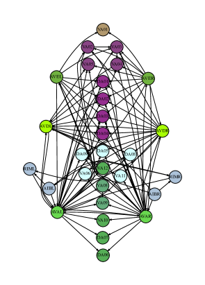
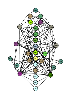
Figure 11: The backward network, colored with the human crafted ground truth from Morone and Makse (2019) (left) and with the equivalence relation obtained by Algorithm 3 (right) with depth 3 (adjusted mutual information is $0.417$).

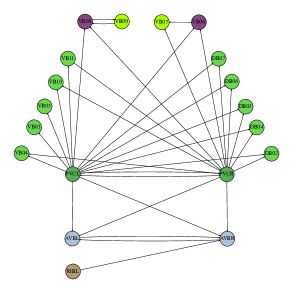
Figure 12: The forward network, colored with the human crafted ground truth from Morone and Makse (2019) (left) and with the equivalence relation obtained by Algorithm 3 (right) with depth 4 (adjusted mutual information is $0.594$).

In this section we shall consider two examples of full reconstruction: we will start from two real-world graph $G$ and apply the whole process described in Section V to both of them. In the case we consider here, the graphs represent two neural circuits controlling the locomotion function of C. elegans as defined in Ref. Morone and Makse (2019): the forward and backward circuits. The backward graph has 30 nodes and 106 arcs, with an average degree of $3.53$; the forward graph has 19 nodes and 35 arcs, with an average degree of $1.84$.

For these datasets, we have a handcrafted ground-truth based on the supposed function of each single node obtained in Morone and Makse (2019); the ground-truth for the backward graph outlines 10 classes with various sizes (the largest class contains 5 nodes, whereas five classes contain 1 or 2 nodes); the ground-truth for the forward graph has 6 classes (the largest class contain 10 nodes, whereas five cases contain 1 ore 2 nodes). The ground-truth is not provided to the algorithm, though, which just starts with the original graph itself.

We tried our experiment with a depth (parameter of Algorithm 3) of 2, 3, 4 and 5. While there is a clear improvement in the performances as the depth increases in the case of the Forward network, the converse seems to happen for the Backward network. An inspection of the logging shows, however, that the number of times the computation of the unordered tree-distance is timed out grows: $60\%$ of the entries are timed out when the depth is $4$ and more than $80\%$ when the depth is $5$. The frequency of this event grows as the depth gets larger, because trees grow in size.

	Backward		Forward
	# clusters	$\operatorname{AMI}$	# clusters	$\operatorname{AMI}$
Depth 2	18	0.262	3	0.423
Depth 3	15	0.417	5	0.500
Depth 4	14	0.398	9	0.594
Depth 5	6	0.355	9	0.594
Cardon-Crochemore	10	0.295	10	0.543

The difference between the ground truth and the equivalence relation obtained at the end is shown in Figure 11 and Figure 12.

Running Algorithm 2, we discover that the total error of the reconstructed quasifibration $\xi:G\to B$ is 18 (three arcs are in excess and fifteen are missing). The final fibration $\xi^{\prime}:G^{\prime}\to B$ obtained by Algorithm 1 modifies the graph $G$ as shown in Figure 13.

Figure 13: The deleted (dashed) and added arcs that should be used to modify the graph $G$ of Figure 11 (right) to turn the coloring into a local in-isomorphism.

VI.2 Synthetic datasets

We ran synthetic experiments as described above, with $n=30$, $v_{\mathrm{m}in}=1$, $v_{\mathrm{m}ax}=5$ and $s=5$, and with depth 2 and 3. Here are the main characteristics of the generated graphs:

	# nodes	# arcs	# classes in the ground truth
Average	$25.5$	$173.7$	$8.5$
Std	$6.5$	$53.9$	$1.7$
Min	$9$	$53$	$4$
Max	$49$	$373$	$15$

As the reader can see, the size, density and number of classes in the ground truth match those of the real-world datasets. Figure 14 shows the boxplot with the performances of the various clustering techniques mentioned above in the case of depth 3. “Reduced UED/OED” is the final result of the algorithm in the paper (after step (4) of Section V is applied) when Unordered/Ordered Edit Distance is used and the silhouette method is applied to obtain the number of clusters. “Agglomerative UED/OED exact” uses the technique of Algorithm 3 but avoids the use of silhouette and directly applies the number of clusters from the ground truth.

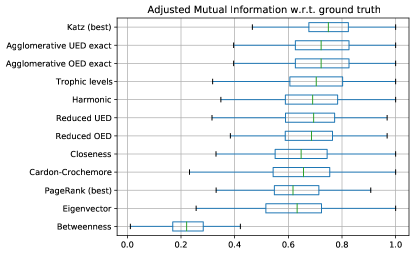
Figure 14: Boxplot with the Adjusted Mutual Information for the clustering generated by various methods; note that the only ones that do not use the number of classes in the ground truth are those called “Reduced UED/OED” and “Cardon-Crochemore”.

It is worth observing that “Reduced UED” is always better than “Cardon-Crochemore”. A more detailed analysis shows that the ratio between “Reduced” and the ground truth outperforms “Cardon-Crochemore” of $19\%$. The discussed behaviour can also be seen in Figure 15, where we produce two heatmaps (one for depth 2 and one for depth 3); each point in each heatmap represents the result of an experiment performed: its X and Y coordinates are the Adjusted Mutual Information of “Cardon-Crochemore” and “Reduced UED”, respectively. We verify that the mass is on or above the diagonal, and that this situation improves as the depth is increased.

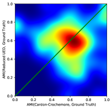
Figure 15: Heatmap showing a comparison between Adjusted Mutual Information for “Cardon-Crochemore” (X axis) and “Reduced UED” (Y axis), for depth 2 (top) and 3 (bottom). The mass is concentrated over the diagonal, and the improvement of “Reduced UED” over “Cardon-Crochemore” increases with the depth (the core moves up).

VII Conclusion

Imperfections in real biological data is a major hurdle in biological network analysis. In this paper we present an approach to dealing with these imperfections via quasifibrations of graphs. We developed a four-step algorithm restoring the graph to a more symmetric version. First, we find the equivalence relations combining "almost" symmetric nodes. Second, we build a quasifibration using the equivalence classes identified in the first step. Third, we construct a graph by modifying a (provably) minimal amount of links in the original graph for which this quasifibration is a fibration. Last, we compute the minimal fibration on the obtained graph to coarsen the obtained result. It was shown analytically that steps 2-4 are performed in an optimal manner. First step is done employing agglomerative clustering.

We used synthetic datasets and real-world datasets studied in Morone and Makse (2019) to fine-tune the clustering method. Performance of the different variations was assessed using AMI (adjusted mutual information). Unordered tree edit-distance accompanied by single linkage with the number of clusters corresponding to the highest value of the Silhouette coefficient have shown the best performance of all considered cases. The algorithm outperformed Cardon-Crochemore by 19% on average on the synthetic networks. On both real networks the algorithm showed a result better than Cardon-Crochemore by comparing outputs with manually curated results in Morone and Makse (2019).

Data Availability Statement

All the algorithms are available at https://github.com/boldip/qf and https://github.com/makselab/QuasiFibrations. All data is available at https://osf.io/amswe.

References

- Morone et al. (2020) F. Morone, I. Leifer, and H. A. Makse, Proceedings of the National Academy of Sciences 117, 8306 (2020).
- Leifer et al. (2020) I. Leifer, F. Morone, S. D. Reis, J. S. Andrade Jr, M. Sigman, and H. A. Makse, PLoS computational biology 16, e1007776 (2020).
- Morone and Makse (2019) F. Morone and H. A. Makse, Nature communications 10, 1 (2019).
- Leifer et al. (2021a) I. Leifer, M. Sánchez-Pérez, C. Ishida, and H. A. Makse, BMC Bioinformatics 22 (2021a).
- Thompson (1917) D. W. Thompson, On Growth and Form (Cambridge University Press, UK, 1917).
- Monod (1969) J. Monod, Symmetry and function of biological systems at the macromolecular level. Proceedings of the 11th Nobel Symposium, Södergarn, Lidingö, Sweden, August 26-29, 1968. A. Engström and B. Strandberg (eds) (Interscience (Wiley), New York, 1969).
- Golubitsky and Stewart (2006) M. Golubitsky and I. Stewart, Bulletin of the american mathematical society 43, 305 (2006).
- DeVille and Lerman (2013) L. DeVille and E. Lerman, arXiv preprint arXiv:1303.3907 (2013).
- Nijholt et al. (2016) E. Nijholt, B. Rink, and J. Sanders, Journal of Differential Equations 261, 4861 (2016).
- Leifer et al. (2021b) I. Leifer, H. A. Makse, D. Phillips, and F. Sorrentino, arXiv preprint (2021b).
- Note (1) Often called an epimorphism in the literature.
- Grothendieck (1960) A. Grothendieck, Seminaire Bourbaki 190 (1959–1960).
- Sachs (1965) H. Sachs, Magyar Tud. Akad. Mat. Kutató Int. Közl. 9, 415 (1965).
- Pisanski et al. (1983) T. Pisanski, J. Shawe–Taylor, and J. Vrabec, J. Combin. Theory Ser. B 35, 12 (1983).
- Boldi and Vigna (2002) P. Boldi and S. Vigna, Discrete Math. 243, 21 (2002).
- Angluin (1980) D. Angluin, in Proc. 12th Symposium on the Theory of Computing (1980) pp. 82–93.
- Note (2) If we assume that is surjective but not injective on the nodes then really has more nodes than , which explains why we call “large” and “small”.
- Note (3) A function between groups is a group homomorphism iff .
- Note (4) Note that, for all , is an automorphism of , that one can apply to both nodes and arcs.
- Norris (1995) N. Norris, Discrete Appl. Math. 56, 61 (1995).
- Berkholz et al. (2017) C. Berkholz, P. Bonsma, and M. Grohe, Theory of Computing Systems 60, 581 (2017).
- Hopcroft (1971) J. Hopcroft, in Theory of machines and computations (Elsevier, 1971) pp. 189–196.
- Cardon and Crochemore (1982) A. Cardon and M. Crochemore, Theoretical Computer Science 19, 85 (1982).
- Paige and Tarjan (1987) R. Paige and R. E. Tarjan, SIAM Journal on Computing 16, 973 (1987).
- Monteiro et al. (2021) H. S. Monteiro, I. Leifer, S. D. Reis, J. S. Andrade Jr, and H. A. Makse, arXiv preprint arXiv:2110.01096 (2021).
- Note (5) is the standard notation used for the symmetric difference of two sets (e.g., ); since in this paper we only need its cardinality, we make an abuse of notation and use for the cardinality of the difference.
- Note (6) We can omit from the objective function the term because it is constant and does not influence minimization.
- Bille (2005) P. Bille, Theoretical computer science 337, 217 (2005).
- Note (7) Although general edit distance is defined for trees with labels on the tree nodes, our trees are unlabelled (equivalently, all tree nodes have the same label), so the only operations allowed are deletion or insertion of a subtree.
- Yoshino et al. (2013) T. Yoshino, S. Higuchi, and K. Hirata, in 2013 Second IIAI International Conference on Advanced Applied Informatics (IEEE, 2013) pp. 135–140.
- Paassen et al. (2015) B. Paassen, B. Mokbel, and B. Hammer, in EDM (2015) p. 632.
- Zhang and Shasha (1989) K. Zhang and D. Shasha, SIAM journal on computing 18, 1245 (1989).
- Nielsen (2016) F. Nielsen, Introduction to HPC with MPI for Data Science (Springer, 2016).
- Note (8) We used the scikit-learn implementation (AgglomerativeClustering).
- Rousseeuw (1987) P. J. Rousseeuw, Journal of computational and applied mathematics 20, 53 (1987).
- Note (9) The problem is very well discussed and no general solution exists Wierzchoń and Kłopotek (2018): in most cases a manual inspection is required (for instance, in the well known “elbow” method). The use of indices like the silhouette coefficient to try to automatize this analysis is certainly error-prone, and may produce suboptimal results.
- Vinh et al. (2010) N. X. Vinh, J. Epps, and J. Bailey, The Journal of Machine Learning Research 11, 2837 (2010).
- Bollobás et al. (2003) B. Bollobás, C. Borgs, J. T. Chayes, and O. Riordan, in SODA, Vol. 3 (2003) pp. 132–139.
- Wierzchoń and Kłopotek (2018) S. T. Wierzchoń and M. A. Kłopotek, Modern algorithms of cluster analysis (Springer, 2018).
- Katz (1953) L. Katz, Psychometrika 18, 39 (1953).
- Boldi and Vigna (2014) P. Boldi and S. Vigna, Internet Math. 10, 222 (2014).