Bayesian Knockoff Generators for Robust Inference Under Complex Data Structure

Abstract

The recent proliferation of medical data, such as genetics and electronic health records (EHR), offers new opportunities to find novel predictors of health outcomes. Presented with a large set of candidate features, interest often lies in selecting the ones most likely to be predictive of an outcome for further study such that the goal is to control the false discovery rate (FDR) at a specified level. Knockoff filtering is an innovative strategy for FDR-controlled feature selection. But, existing knockoff methods make strong distributional assumptions that hinder their applicability to real world data. We propose Bayesian models for generating high quality knockoff copies that utilize available knowledge about the data structure, thus improving the resolution of prognostic features. Applications to two feature sets are considered: those with categorical and/or continuous variables possibly having a population substructure, such as in EHR; and those with microbiome features having a compositional constraint and phylogenetic relatedness. Through simulations and real data applications, these methods are shown to identify important features with good FDR control and power.

1 Introduction

The proliferation of biomedical data made available in the past two decades, such as genetics and electronic health records (EHR), offers new opportunities to identify novel predictors of an individual’s health outcomes. Yet, this abundance also presents formidable challenges to accurately detecting these factors. Among a large number of candidate features, usually a large proportion are expected to have a negligible effect on the outcome and interest lies in selecting just the ones most likely to be predictive, so the goal is often to control the false discovery rate (FDR) (Benjamini and Hochberg,, 1995) at a prespecified level. Penalized regression models, such as the lasso (Tibshirani,, 1996), are often employed for feature selection. However, performing formal hypothesis testing of the effects of predictors and controlling the false discovery rate (FDR) are generally quite challenging for these procedures.

Knockoff filtering is a cutting-edge strategy that can select features while maintaining FDR control. This approach proceeds as follows. First, for each candidate feature $X_{j}$ a knockoff copy $\tilde{X}_{j}$ is constructed such that the the knockoff feature is approximately identically distributed to the original one but is independent of the outcome. Second, the influences of the original and knockoff features on the outcome are evaluated using quantities called importance statistics, such as the lasso penalty parameter at which a feature enters the model; the independence of each knockoff feature from the outcome allows it to serve as a negative control for its corresponding original feature when assessing the original feature’s influence. Third, features are selected based on the importance statistics such that the FDR is controlled at the specified level. An advantage of this approach is that FDR control is maintained for finite samples, avoiding reliance on asymptotic properties. Although this procedure is straightforward, the construction of suitable knockoff features is nontrivial. The original knockoff procedure (Barber and Candès,, 2015), called Fixed-X, constructs knockoffs deterministically from the observed data and is applicable only when the number of features does not exceed the sample size ($p\leq n$). A subsequent development (Candes et al.,, 2018) generates knockoffs randomly by modeling the distribution of the original features, an approach called Model-X. But, the Model-X procedure in Candes et al., (2018) assumes a Gaussian distribution for features, an assumption that is often violated in real life applications, such as for EHR, genetics, and microbiome data.

Categorical variables frequently arise in clinical research, particularly with questionnaires, registries, and EHR. Modeling the impact of categorical covariates on an outcome often requires creating dummy variables that are mutually exclusive, and so it is desirable to include or exclude dummy variables of the same group all at once in the feature selection procedure. Dai and Barber, (2016) proposed an extension of the Model-X knockoff filter that can perform FDR-controlled selection among grouped continuous features. Like the Model-X procedure, however, this grouped variable extension assumes a joint Gaussian distribution for the features, which may be a poor approximation of the true data structure and can give poor inference. This may be especially problematic in common situations where binary or categorical features are considered. We instead propose Bayesian models that can closely mimic the feature structure and the mutual exclusivity of dummy variables, thereby producing high quality knockoffs for FDR-controlled variable selection among categorical features.

High dimensional continuous data arises increasingly frequently in the study of genetic and cellular features that may be prognostic for disease development. Three challenges that arise in the analysis of these data include computational burden in handling the large dimensionality; accounting for the potentially complex distributions of the features and their correlations; and the potential existence of a population substructure such that the observations arise from a mixture distribution, such as EHR data from multiple treatment centers or genetics data from patients with various disease subtypes. The assumption of a Gaussian distribution for the features is unrealistic in these settings and may produce poor feature selection if employed. To overcome this limitation and allow for additional flexibility in modeling, Gimenez et al., (2019) proposed the use of a finite mixture of Gaussian distributions to construct knockoff copies. This should provide more robust knockoff generation due to the fact that, with a sufficiently large number of mixture components, any continuous distribution may be estimated arbitrarily closely by a mixture of Gaussians. These models require prespecification of the number of components, however, a parameter for which little information may be available a priori. A Dirichlet Process Mixture (DPM) of Gaussian distributions (Lo,, 1984) avoids this requirement by automatically selecting both the number of mixture components and their parameters based on the observed data, leading to its successful application in accurate density estimation for multidimensional continuous data. We propose to utilize a Gaussian DPM model to generate real-valued knockoff features, offering flexible, yet accurate modeling that can fully capture the complexity of arbitrary data distributions.

In recent years, the microbiome has increasingly gained recognition in the medical field for the role it plays in human health; moreover, next-generation sequencing technologies now permit direct quantification of the microbiome composition in a given sample. Substantial challenges arise in microbiome data analysis, though. In addition to suffering from the curse of dimensionality common to genetics data, microbiome data also have a phylogenetic structure and the compositional constraint that the abundances of all taxa must sum to one, making general feature selection methods unsuitable. Previously, Srinivasan et al., (2020) proposed a two-step knockoff filter that first implements a compositional screening procedure to decrease the dimension and then applies a Fixed-X knockoff filter. We propose an alternative approach that uses Bayesian models to generate knockoffs for microbiome features and apply a modified compositional lasso model to achieve feature selection directly.

This paper proposes using Bayesian methodology to generate knockoff copies, taking full advantage of available knowledge about the data structure. In summary, we first build a Bayesian model for the covariates’ distribution based on existing knowledge of the covariates’ distributions. Secondly, the observed covariate data are used to estimate the parameters of the model through MCMC, thereby learning about the covariates’ true distribution. Finally, the saved parameters from MCMC iterations are used to sample knockoff copies, which should resemble the true feature distribution much more closely than the knockoff copies generated by the original knockoff method. We illustrate this approach with three models: (1) a parametric model for data with categorical covariates, (2) a nonparametric Dirichlet process mixture of Gaussians model for high dimensional continuous features, and (3) a parametric model for microbiome data with a compositional constraint.

The paper is structured as follows. Section 2 presents our formulation and implementation for feature selection among categorical covariates using a parametric Bayesian model. In section 3, we describe our method for knockoff filtering of high dimensional continuous data using a Dirichlet process mixture model. Section 4 proposes a parametric Bayesian model to generate knockoffs for microbiome data and a corresponding compositional lasso model for knockoff feature selection among these data. Section 5 presents a simulation study that evaluates our Bayesian knockoff generators and compares their performance with existing knockoff methods. Section 6 implements applications of our methods to feature selection on real world datasets. Section 7 concludes the paper with a brief discussion.

2 Bayesian Knockoff Generator for Categorical Covariates

2.1 Knockoff Generator Model Specification

Assume there are $n$ observations and $J$ categorical covariates. The $j^{th}$ categorical covariate is assumed to have $m_{j}+1$ categories; these correspond to binary dummy variables, $\mathbf{X}_{j_{0}},\mathbf{X}_{j_{1}},\mathbf{X}_{j_{2}},\dots,\mathbf{X}_{j_{m_{j}}}$, where $\mathbf{X}_{j_{0}}$ represents the reference group. Because continuous covariates are also often present, we assume $C$ continuous covariates are included in the dataset, denoted by $\mathbf{X}_{c}$, $c=1,2,\dots,C$. After standardizing the continuous covariates, we specify our model as the following:

$$\begin{split}(X_{i,j_{0}},X_{i,j_{1}},X_{i,j_{2}},\dots,X_{i,j_{m_{j}}})|X_{i,j_{.}}=1&\sim\mathrm{Multinomial}(\theta_{j_{0}},\theta_{j_{1}},\theta_{j_{2}},\dots\theta_{j_{m_{j}}}),\quad j=1,2,\dots J,\quad i=1,2,\dots,n,\\ (Z_{j_{1}},Z_{j_{2}},\dots,Z_{j_{m_{j}}})&=(\log(\theta_{j_{1}}/\theta_{j_{0}}),\dots,\log(\theta_{j_{m_{j}}}/\theta_{j_{0}})),\\ (X_{i,1},X_{i,2},\dots,X_{i,C})&\sim\mathrm{No}((Z_{1},Z_{2},\dots,Z_{C}),\tau\mathbf{I}),\\ (Z_{1},Z_{2},\dots,Z_{C},Z_{1_{1}},Z_{1_{2}},\dots,Z_{J,m_{J}})&\sim\mathrm{No}(\mathbf{0},\boldsymbol{\Omega}),\\ \boldsymbol{\Omega}&\sim\mathrm{Wishart}(\boldsymbol{\Omega}_{0},p),\\ \tau&\sim\mathrm{Gamma}(\tau_{a},\tau_{b}).\end{split}$$ (1)

Here $X_{i,j_{.}}$ is the sum of the dummy variables for the $j$th categorical covariate of the $i$th observation, which is always equal to $1$. The probabilities of each category for the $j$th categorical covariate are $\theta_{j_{0}},\theta_{j_{1}},\theta_{j_{2}},\dots,\theta_{j_{m_{j}}}$, which sum up to $1$; moreover, $Z_{j_{1}},Z_{j_{2}},\dots,Z_{j_{m_{j}}}$ represent the log probability ratios compared with the reference group for each category. The continuous covariates are assumed to come from a multivariate Gaussian with mean $(Z_{1},Z_{2},\dots,Z_{C})$ and precision matrix $\tau I$. The vector $\mathbf{Z}=(Z_{1},Z_{2},\dots,Z_{C},Z_{1_{1}},Z_{1_{2}},\dots,Z_{J_{m_{J}}})$ is from a multivariate Gaussian distribution, which has a $\mathbf{0}$ vector mean and a precision matrix generated from a Wishart distribution. To give a non-informative prior, we set $\tau_{a}=0.001$, $\tau_{b}=0.001$ and $\boldsymbol{\Omega}_{0}=\mathrm{diag}(0.1/(p-1))$, where $p=\dim(\mathbf{Z})$. MCMC methods can be used to draw a sample from the posterior of $\mathbf{Z}$ and $\tau$ and subsequently simulate the knockoff copies $\tilde{\mathbf{X}}$ according to model (1), using Rstan for instance.

2.2 Group Lasso and Group Variable Filtering

Our goal is to identify features among a collection of candidates that are prognostic for a continuous outcome. Let $y_{i}$ be the outcome value for the $i^{th}$ observation. Since each categorical variable corresponds to a group of dummy binary variables, we want to ensure features of these groups are selected or excluded simultaneously. We adopt Yuan and Lin, (2006)’s group lasso model to promote this selection. The model is expressed as $\mathbf{Y}=\mathbf{X}\boldsymbol{\beta}+\boldsymbol{\epsilon},\boldsymbol{\epsilon}\sim\mathrm{N(\mathbf{0},\sigma^{2}\mathbf{I})},$ subject to

$$\hat{\boldsymbol{\beta}}=\operatorname*{arg\,min}_{\boldsymbol{\beta}}\bigg{\{}{\parallel\mathbf{Y}-\mathbf{X}\boldsymbol{\beta}\parallel}^{2}_{2}+\lambda\sum^{M}_{m=1}\sqrt{p_{m}}{\parallel\boldsymbol{\beta}_{m}\parallel}_{2}\bigg{\}},$$

where $\mathbf{X}$ is the full matrix of dummy binary and continuous covariates, $\boldsymbol{\beta}_{m}$ is the vector of coefficients for group $m$, $p_{m}$ is the group size, and $\lambda$ is the group lasso penalty parameter. Each continuous covariate is treated as a group of size one and the total number of groups is the number of continuous covariates plus the number of categorical covariates $M=C+J$.

The group false discovery rate is defined as the expected proportion of selected groups which are actually false discoveries. For the group lasso model, this may be expressed as

$$\text{FDR}_{\text{group}}=\mathbb{E}\bigg{[}\dfrac{\#\{m:\boldsymbol{\beta}_{m}=\mathbf{0},m\in\hat{S}\}}{\#\{m:m\in\hat{S}\}\vee 1}\bigg{]},$$

where $\hat{S}=\{m:\hat{\boldsymbol{\beta}}_{m}\neq\mathbf{0}\}$ is the set of all selected group of features ($\vee$ denotes the maximum of two numbers).

After constructing the group knockoff copies $\tilde{\mathbf{X}}$ from MCMC results, we apply Dai and Barber, (2016)’s group knockoff filter to select groups of features. This involves repeatedly applying the group lasso across a range of $\lambda$ values to the concatenated vector of original and knockoff features $(\mathbf{X},\tilde{\mathbf{X}})$ and recording the following information for each of the 2M total groups:

$$\lambda_{m}=\sup\{\lambda:\hat{\boldsymbol{\beta}}_{m}\neq\mathbf{0}\},\quad\tilde{\lambda}_{m}=\sup\{\lambda:\hat{\boldsymbol{\beta}}_{m+M}\neq\mathbf{0}\}\quad m=1,\cdots,M.$$

$\lambda_{m}$ and $\tilde{\lambda}_{m}$ represent the largest group lasso penalty parameter values at which the $m^{th}$ original and corresponding knockoff feature groups enter the model, respectively, and are used as importance measures for these groups. For each value of $\lambda$, we can compute

$$\hat{S}(\lambda)=\{m:\lambda_{m}>(\tilde{\lambda}_{m}\vee\lambda)\}\quad\mbox{and}\quad\tilde{S}(\lambda)=\{m:\tilde{\lambda}_{m}>(\lambda_{m}\vee\lambda)\},$$

where $\hat{S}(\lambda)$ is the set of selected groups of features in the original data that enter the model earlier, at larger $\lambda$ values, than the corresponding knockoff feature groups when the group lasso is applied at penalty level $\lambda$, whereas $\tilde{S}(\lambda)$ is the set of selected groups of features in the knockoff copies that enter the model earlier than the original features. To control the false discovery rate (FDR) at a given level, we need to control the proportion of original features that are falsely selected, i.e. control the membership of $\hat{S}(\lambda)$. For a given $\lambda$ value, the false discovery proportion (FDP) can be estimated as:

$$\text{FDP}(\lambda)\approx\widehat{\text{FDP}}(\lambda)=\dfrac{|\tilde{S}(\lambda)|}{|\hat{S}(\lambda)|\vee 1},$$

where $|\tilde{S}(\lambda)|$ stands for the cardinality of set of selected knockoff groups, which serves as an estimate of the number of false discoveries as the covariate group $\mathbf{X}_{j}$ and its knockoff copy $\tilde{\mathbf{X}}_{j}$ are equally likely to enter the model if the $j^{th}$ covariate is a null feature, i.e. $\boldsymbol{\beta}_{j}=\mathbf{0}$. $|\hat{S}(\lambda)|$ stands for the cardinality of set of selected original groups, that is number of selected original group of features. A more conservative estimate of the FDP can be obtained by adding $1$ to the numerator:

$$\text{FDP}(\lambda)\approx\widehat{\text{FDP}}_{+}(\lambda)=\dfrac{1+|\tilde{S}(\lambda)|}{|\hat{S}(\lambda)|\vee 1},$$

Given a prespecified false discovery rate $q$, the estimate of the smallest penalty parameter value that maintains FDR control at level $q$ is

$$\hat{\lambda}=\min\{\lambda:\widehat{\text{FDP}}(\lambda)\leq q\}.$$

The set of features selected by the group knockoff filter is then $\hat{S}(\hat{\lambda})$. As shown by Dai and Barber, (2016), this selection procedure provides control of a modified form of the FDR. If instead the more conservative FDP estimate $\text{FDP}(\lambda)\approx\widehat{\text{FDP}}_{+}(\lambda)$ is used to compute $\hat{\lambda}$, control of the ordinary FDR is provided; using the procedure with the conservative estimate of FDP is often called “knockoff+” filtering.

3 Bayesian Knockoff Generator for Continuous Features from Mixture Distributions

3.1 Knockoff Generator Model Specification

The Gaussian Dirichlet Process Mixture (GDPM) model is a useful tool for modeling the potentially complex data distribution of high dimensional continuous data vectors. We utilize the GDPM model for knockoff generation in this context by estimating the distribution of the features $\mathbf{X}$ and then generating knockoff copies $\tilde{\mathbf{X}}$ from the estimated distribution. A multivariate Gaussian distribution can be parameterized by its associated mean vector and precision matrix, denoted as the pair $\boldsymbol{\theta}=(\boldsymbol{\mu},\boldsymbol{\Omega})$ taking values in the set $\{(\mathbf{a},\mathbf{B}):\mathbf{a}\in\mathbb{R}^{p},\mathbf{B}\in\mathbb{R}^{p\times p}\mbox{ is positive definite}\}$. The GDPM model specifies that the rows $\mathbf{X}_{i}$ of the data matrix $\mathbf{X}_{n\times p}$ arise from an infinite mixture of these distributions, specified by the following hierarchical model:

$$\begin{split}\mathbf{X}_{i}|\boldsymbol{\theta}_{i}&\overset{iid}{\sim}\mathrm{No}(\boldsymbol{\mu}_{i},\boldsymbol{\Omega}_{i}),\quad i=1,\dots,n,\\ (\boldsymbol{\mu}_{i},\boldsymbol{\Omega}_{i})&\overset{ind}{\sim}G,\\ G&\sim\mathrm{DP}(G_{0},\alpha),\\ G_{0}&=\mathrm{NoWi}(\mathbf{m},k,\mathbf{W},v),\\ \end{split}$$ (2)

$DP(G_{0},\alpha)$ is a Dirichlet process with base distribution $G_{0}$ and concentration parameter $\alpha$. $G_{0}$ is given a Normal-Wishart distribution, which is conjugate to multivariate Gaussian data distribution. To be precise, if $(\mathbf{u},\mathbf{V})\sim\mathrm{NoWi}(\mathbf{m},k,\mathbf{W},v)$, then $\mathbf{V}\sim\mathrm{Wishart}(\mathbf{W},v)$ has scale matrix $\mathbf{W}$, degrees of freedom $v$ and $\mathbf{u}|\mathbf{V}\sim\mathrm{No}(\mathbf{m},k\mathbf{V})$ has mean $\mathbf{m}$, precision matrix $k\mathbf{V}$. The concentration parameter $\alpha$ controls how much variability arises in the distributions generated by the Dirichlet process, with higher $\alpha$ giving less variability and distributions that are ”closer” to $G_{0}$. The $G$ distribution generated by the DP process is discrete, causing some of the $\boldsymbol{\theta}_{i}=(\boldsymbol{\mu}_{i},\boldsymbol{\Omega}_{i})$’s to be equal so that some data vectors will share a common component $\mathrm{No}(\boldsymbol{\mu}_{i},\boldsymbol{\Omega}_{i})$ in the posterior distribution. Thus, the posterior distribution of the $\mathbf{X}_{i}$’s is likely to have fewer mixture components than there are data points, with the number of components being informed by the data.

Let $c_{i}$ denote the class label for the $i^{th}$ observation. Note that the exact values of these are unimportant, as they only identify which $\boldsymbol{\theta}_{i}$ lie within the same component; without loss of generality, we can assume all $c_{i}\in\{1,...,n\}$. Because the base distribution $G_{0}$ is specified as Normal-Wishart, which is conjugate to the Gaussian distribution, the Collapsed Gibbs sampler proposed by Neal, (2000) can be used to obtain posterior draws of the $\boldsymbol{\theta}_{i}$. At each MCMC iteration, class assignments are selected for each data point according to the following Gibbs conditionals:

$$P(c_{i}=c|\mbox{ all }c_{j}\neq c_{i},\mathbf{X}_{1},\dots,\mathbf{X}_{n}) =b\cdot\frac{n_{-i,c}}{n-1+\alpha}\int f(\mathbf{X}_{i}|\boldsymbol{\theta})dH_{-i,c}(\boldsymbol{\theta})\mbox{ for }c\in\{c_{1},\dots,c_{i-1}\},$$

$$P(c_{i}\neq c_{j}\mbox{ for all }j\neq i|\mbox{ all }c_{j}\neq c_{i},\mathbf{X}_{1},\dots,\mathbf{X}_{n}) =b\cdot\frac{\alpha}{n-1+\alpha}\int f(\mathbf{X}_{i}|\boldsymbol{\theta})dG_{0}(\boldsymbol{\theta}),$$

where $n_{-i,c}=|j:j\neq i,c_{j}=c|$ is the number of observations in cluster $c$ distinct from observation $i$, $H_{-i,c}(\boldsymbol{\theta})$ is the posterior CDF of $G_{0}$ given all $\mathbf{X}_{j}$ for which $j\neq i$ and $c_{j}=c$, and b is a normalizing constant. Because of the conjugacy of $G_{0}$ to the data density $f$, the $H_{-i,c}$ are also conjugate and so the integrals can be computed directly.

The prior elicitation for GDPM models can be challenging in general; the presence of high dimensional data greatly complicates this task. When $p\to\infty$ as $n$ remains fixed, Chandra et al., (2020) showed that there is a tendency for the posterior predictive distribution to converge to either a single mixture component or $n$ distinct components, neither of which may approximate the true data distribution well. As a general approach to this problem for datasets of arbitrary scales and distributions, we recommend the approach suggested by Shi et al., (2019), summarized in the following steps:

1. Linearly transform the data vectors $\mathbf{X}_{i}$ to $\mathbf{Z}_{i}$ in a manner so that, approximately, the $\mathbf{Z}_{i}$ have zero mean and unit variance

2. Apply the GDPM model to the $\mathbf{Z}_{i}$ with a specific choice of hyperparameters (given below) and obtain posterior inference on their data distribution

3. Back-transform the inference to obtain inference on the original data $\mathbf{X}_{i}$

At Step 2 of this procedure, we recommend using these values for the hyperparameters $\mathbf{m},k,\mathbf{W}$, and $v$:

$$\mathbf{m}=\mathbf{0},\quad v=p+2p^{2}/n,\quad k=\frac{vn\chi^{2}(p,\psi)(1-\psi)}{(v-p-1)(n-1)p},\quad\mathbf{W}=v\mathbf{I},\quad\psi=0.99,$$

where $\chi^{2}(p,\psi)$ is the $\psi^{th}$ quantile of the $\chi^{2}$ distribution with $p$ degrees of freedom. These values appear to work well when $n,p\leq 250$ and were obtained using a combination of the method of moments approach in Shi et al., (2019) and experimentation with high dimensional examples.

3.2 Knockoff Generation and Filtering

Using the model specification in Section 3.1, posterior MCMC samples can be obtained for the class assignments $c_{i}$ of the data vectors $\mathbf{X}_{i}$. Given these class assignments, posterior samples can be drawn for the parameters $\boldsymbol{\theta}_{i}$ as $\boldsymbol{\theta}_{i}\sim H_{i}$, where $H_{i}$ is the posterior distribution of $G_{0}$ given all data vectors in class $c_{i}$, i.e. $\mathbf{X}_{j}$ with $c_{j}=c_{i}$. Then the fitted GDPM model for the data distribution is simply $\sum_{i=1}^{n}n^{-1}\mathrm{No}(\boldsymbol{\mu}_{i},\boldsymbol{\Omega}_{i})$. Each MCMC iteration provides a fitted model for the data from which a set of knockoff copies may be generated. Therefore, it suffices to save just one iteration after the MCMC chain reaches convergence to the posterior.

Any choice of knockoff importance statistic may be applied using knockoffs generated from the GDPM model, provided that the statistic satisfies the antisymmetry property (Candes et al.,, 2018). For the simulations presented in Section 5, we consider the lasso signed max (LSM) importance statistic, defined for the $j^{th}$ feature as

$$W_{j}=(\text{largest }\lambda\text{ such that }\mathbf{X}_{j}\text{ or }\tilde{\mathbf{X}}_{j}\text{ enters lasso model})\times\begin{cases}+1&\text{if }\mathbf{X}_{j}\text{ enters before }\tilde{\mathbf{X}}_{j},\\ -1&\text{if }\tilde{\mathbf{X}}_{j}\text{ enters before }\mathbf{X}_{j}.\\ \end{cases}$$ (3)

4 Bayesian Knockoff Generator for Microbiome Data

4.1 Knockoff Generator Model Specification

Advances in next-generation sequencing from the past decade enable researchers to cheaply and comprehensively analyze microbial communities, with most microbiome studies rely on sequencing of the 16S ribosomal RNA (16S rRNA) marker gene. When analyzing microbiome data, the first step usually is to group observed sequences of this gene into operational taxonomic units (OTUs) based on similarity using specially-designed processing pipelines. Then often the representative sequences of OTUs are compared to existing databases and the OTUs are assigned according to a known taxonomic classification (taxa), which goes in the order of kingdom, phylum, class, order, family, genus and species, from broad to specific. The taxonomy classification naturally forms a tree structure that can help describing the evolutionary relationships between bacteria. Often, OTUs are considered the taxonomic units with the highest resolution in 16S rRNA microbiome data and are represented by tip nodes in a phylogenetic tree. For a specified taxonomic level (say genus), the taxa count matrix for $n$ observations and $p$ taxa is denoted as a $\mathbf{X}_{n\times p}$ matrix, where the $i^{th}$ row $\mathbf{X}_{i}$ is a vector of taxa counts for the $i^{th}$ observation. We generate knockoffs for microbiome features using the model described below, inspired by Vannucci, (2020):

$$\begin{split}\mathbf{X}_{i}|X_{i,.}&\sim\mathrm{Multinomial}(\boldsymbol{\theta}),\quad i=1,2,\dots,n,\\ \boldsymbol{\theta}&=\mathrm{softmax}(\boldsymbol{\mu}),\quad\mu_{1}=0,\\ \boldsymbol{\mu}_{-1}&\sim\mathrm{No}(\mathbf{0},\boldsymbol{\Omega}),\\ \boldsymbol{\Omega}&\sim\mathrm{Wishart}(\boldsymbol{\Omega}_{0},p-1).\end{split}$$

Here $X_{i,.}$ is the sum of taxa counts for the $i^{th}$ observation, and $\boldsymbol{\theta}$ is the probability vector for the multinomial distribution, which sums to one. We model $\boldsymbol{\theta}$ as the result of a softmax function with $\boldsymbol{\mu}$ as input. Fixing the first parameter of $\boldsymbol{\mu}$ to be $0$, we give the other $p-1$ parameters a multivariate Gaussian prior with a $\mathbf{0}$ vector mean and precision matrix $\boldsymbol{\Omega}$. We add a hierarchy by giving $\boldsymbol{\Omega}$ a $\mathrm{Wishart}(\boldsymbol{\Omega}_{0},p-1)$ prior. To give the model a non-informative prior, we set $\boldsymbol{\Omega}_{0}=\mathrm{diag}(0.1/(p-1))$. MCMC methods can be used to sample the posterior of $\boldsymbol{\theta}$ and subsequently simulate the knockoff copies $\tilde{\mathbf{X}}$ with the total count for each knockoff vector $\tilde{\mathbf{X}}_{i}$ equaling the total $X_{i,.}$ across original features; Rstan can be applied for posterior sampling from this model.

4.2 Modified Compositional Lasso Model for Microbiome Knockoff Selection

We first convert the matrix of raw sequence counts $\mathbf{X}_{n\times p}$ into a matrix of relative abundances $\mathbf{A}_{n\times p}$ such that $A_{ij}=X_{ij}/X_{i,.}$. Due to the compositional constraint, each row of $\mathbf{A}$ must sum up to one. One approach to handling this sum to one constraint is to choose one column (say the $p^{th}$ column) as the reference taxa and analyze the log-transformed relative abundances $Q_{ij}=\log(A_{ij}/A_{ip})$, where $i=1,2,\dots,n$ and $j=1,2,\dots,p-1$; to account for the possibility of zero taxa counts, common practice is add $0.5$ to taxa with zero counts before computing the abundance matrix from the count matrix. Denoting the outcomes by an $n$ dimensional vector $\mathbf{Y}$, one can construct a linear model with the $n\times(p-1)$ matrix $\mathbf{Q}$, $\mathbf{Y}=\mathbf{Q}\boldsymbol{\beta}+\boldsymbol{\epsilon}$, where $\boldsymbol{\epsilon}\sim\mathrm{No(\mathbf{0},\tau\mathbf{I})}.$

To avoid picking a reference taxa, Lin et al., (2014) instead proposed appending a coefficient $\beta_{p}=-\sum_{j=1}^{p-1}\beta_{j}$ at the end of the $p-1$ vector $\boldsymbol{\beta}$, thereby converting this log-contrast model to a model with a coefficients sum-to-zero constraint,

$$\mathbf{Y}=\mathbf{Z}\boldsymbol{\beta}+\boldsymbol{\epsilon},\quad\boldsymbol{\epsilon}\sim\mathrm{No(\mathbf{0},\tau\mathbf{I})},\text{ subject to}\sum_{j=1}^{p}\beta_{j}=0,$$

where elements of the matrix $\mathbf{Z}$ are the log taxa abundances $Z_{ij}=\log(A_{ij})$.

To perform knockoff feature selection among the taxa, we apply this model to the combined log abundance matrix of the original and the knockoff $\mathbf{C}=[\mathbf{Z},\tilde{\mathbf{Z}}]$, where the knockoff abundances $\tilde{\mathbf{Z}}$ are computed using the knockoff taxa counts $\tilde{\mathbf{X}}$ generated as is Section 4.1. A naive lasso is not applicable due to the sum-to-zero constraints on the coefficients of both the original and knockoff abundances. Instead, we apply a modification of the compositional lasso (Lin et al.,, 2014) that enforces these restrictions. The optimization problem can be stated as:

$$\hat{\boldsymbol{\beta}}=\operatorname*{arg\,min}_{\boldsymbol{\beta}}(\frac{1}{2N}\parallel\mathbf{Y}-\mathbf{C}\boldsymbol{\beta}\parallel_{2}^{2}+\lambda\parallel\boldsymbol{\beta}\parallel_{1}),\quad\text{subject to }\mathbf{1}_{1\times p}^{T}\boldsymbol{\beta}_{o}=0,\quad\mathbf{1}_{1\times p}^{T}\boldsymbol{\beta}_{k}=0,\quad$$ (4)

where $\boldsymbol{\beta}_{o}$ and $\boldsymbol{\beta}_{k}$ are the respective vectors of coefficients for the original and knockoff features such that $\boldsymbol{\beta}=(\boldsymbol{\beta}_{o},\boldsymbol{\beta}_{k})$. The problem can be solved with c-lasso solver in Python (Simpson et al.,, 2021).

One choice of knockoff importance statistic is the largest penalty parameter at which a covariate enters the model, defined as

$$W_{j}=(\text{largest }\lambda\text{ such that }\mathbf{Z}_{j}\text{ or }\tilde{\mathbf{Z}}_{j}\text{ enters lasso model})\times\begin{cases}+1&\text{if }\mathbf{Z}_{j}\text{ enters before }\tilde{\mathbf{Z}}_{j},\\ -1&\text{if }\tilde{\mathbf{Z}}_{j}\text{ enters before }\mathbf{Z}_{j}.\\ \end{cases}$$ (5)

This is analogous to the LSM statistic used for an ordinary lasso model. Other importance statistics could also be used provided they possess the antisymmetry property.

4.3 Incorporating Phylogenetic Information

Given the phylogenetic tree information, the proposed method can also be used to select tree nodes that are predictive of the outcomes. Recently, Bien et al., (2021) incorporated phylogenetic tree structure in order to aggregate rare features in lasso modeling, representing the coefficient vector $\boldsymbol{\beta}$ as a product of a binary matrix $\mathbf{T}$ describing the structure of the tree and a vector $\boldsymbol{\gamma}$ of the effects of the tree nodes. Each column of $\mathbf{T}$ corresponds to a tree node, while each row of $\mathbf{T}$ corresponds to an OTU. The constraint $\boldsymbol{\beta}=\mathbf{T}\boldsymbol{\gamma}$ expresses the relationship that the effect of each tip node is the sum of the effects of itself and all higher taxonomic units to which it belongs.

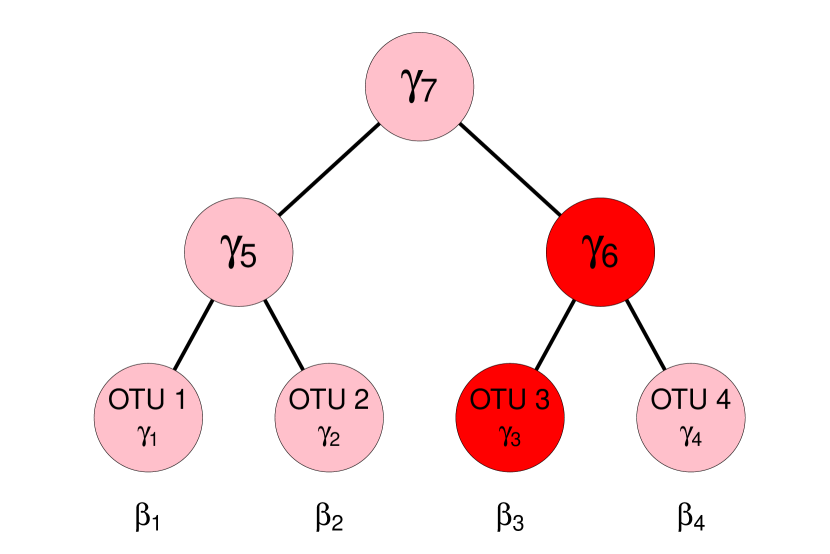
Figure 1: Schematic plot of feature aggregation

$$\mathbf{T}=\hbox{}\vbox{\kern 0.86108pt\hbox{$\kern 0.0pt\kern 2.5pt\kern-5.0pt\left(\kern 0.0pt\kern-2.5pt\kern-6.66669pt\vbox{\kern-0.86108pt\vbox{\vbox{ \halign{\kern\arraycolsep\hfil\@arstrut$\kbcolstyle#$\hfil\kern\arraycolsep& \kern\arraycolsep\hfil$\@kbrowstyle#$\ifkbalignright\relax\else\hfil\fi\kern\arraycolsep&& \kern\arraycolsep\hfil$\@kbrowstyle#$\ifkbalignright\relax\else\hfil\fi\kern\arraycolsep\cr 5.0pt\hfil\@arstrut$\scriptstyle$\hfil\kern 5.0pt&5.0pt\hfil$\scriptstyle\gamma_{1}$\hfil\kern 5.0pt&5.0pt\hfil$\scriptstyle\gamma_{2}$\hfil\kern 5.0pt&5.0pt\hfil$\scriptstyle\gamma_{3}$\hfil\kern 5.0pt&5.0pt\hfil$\scriptstyle\gamma_{4}$\hfil\kern 5.0pt&5.0pt\hfil$\scriptstyle\gamma_{5}$\hfil\kern 5.0pt&5.0pt\hfil$\scriptstyle\gamma_{6}$\hfil\kern 5.0pt&5.0pt\hfil$\scriptstyle\gamma_{7}\\\beta_{1}$\hfil\kern 5.0pt&5.0pt\hfil$\scriptstyle 1$\hfil\kern 5.0pt&5.0pt\hfil$\scriptstyle 0$\hfil\kern 5.0pt&5.0pt\hfil$\scriptstyle 0$\hfil\kern 5.0pt&5.0pt\hfil$\scriptstyle 0$\hfil\kern 5.0pt&5.0pt\hfil$\scriptstyle 1$\hfil\kern 5.0pt&5.0pt\hfil$\scriptstyle 0$\hfil\kern 5.0pt&5.0pt\hfil$\scriptstyle 1\\\beta_{2}$\hfil\kern 5.0pt&5.0pt\hfil$\scriptstyle 0$\hfil\kern 5.0pt&5.0pt\hfil$\scriptstyle 1$\hfil\kern 5.0pt&5.0pt\hfil$\scriptstyle 0$\hfil\kern 5.0pt&5.0pt\hfil$\scriptstyle 0$\hfil\kern 5.0pt&5.0pt\hfil$\scriptstyle 1$\hfil\kern 5.0pt&5.0pt\hfil$\scriptstyle 0$\hfil\kern 5.0pt&5.0pt\hfil$\scriptstyle 1\\\beta_{3}$\hfil\kern 5.0pt&5.0pt\hfil$\scriptstyle 0$\hfil\kern 5.0pt&5.0pt\hfil$\scriptstyle 0$\hfil\kern 5.0pt&5.0pt\hfil$\scriptstyle 1$\hfil\kern 5.0pt&5.0pt\hfil$\scriptstyle 0$\hfil\kern 5.0pt&5.0pt\hfil$\scriptstyle 0$\hfil\kern 5.0pt&5.0pt\hfil$\scriptstyle 1$\hfil\kern 5.0pt&5.0pt\hfil$\scriptstyle 1\\\beta_{4}$\hfil\kern 5.0pt&5.0pt\hfil$\scriptstyle 0$\hfil\kern 5.0pt&5.0pt\hfil$\scriptstyle 0$\hfil\kern 5.0pt&5.0pt\hfil$\scriptstyle 0$\hfil\kern 5.0pt&5.0pt\hfil$\scriptstyle 1$\hfil\kern 5.0pt&5.0pt\hfil$\scriptstyle 0$\hfil\kern 5.0pt&5.0pt\hfil$\scriptstyle 1$\hfil\kern 5.0pt&5.0pt\hfil$\scriptstyle 1$\hfil\kern 5.0pt\crcr}}}}\right)$}}$$

Figure 1 illustrates the aggregation of features using a phylogeny tree, with the red color denoting two selected nodes under consideration, nodes 3 and 6. The corresponding structure matrix $\mathbf{T}$ is shown to the right of the schematic plot. The effect of OTU 3 is the sum of the effects of node 3 and 6, i.e. $\beta_{3}=\gamma_{3}+\gamma_{6}$, while only node 6 contributes to the effect of OTU 4, $\beta_{4}=\gamma_{6}$. The effects of the other two OTUs are not dependent on nodes 3 and 6 as these selected nodes do not lie along the OTUs’ paths to the tree origin selected. Condition on the phylogenetic tree structure, the optimization goal becomes

$$\hat{\boldsymbol{\beta}}=\operatorname*{arg\,min}_{\boldsymbol{\beta}}(\frac{1}{2N}\parallel\mathbf{Y}-\mathbf{C}\boldsymbol{\beta}\parallel_{2}^{2}+\lambda\parallel\boldsymbol{\gamma}\parallel_{1}),\quad\text{subject to }\mathbf{1}_{1\times p}^{T}\boldsymbol{\beta}_{o}=0,\quad\mathbf{1}_{1\times p}^{T}\boldsymbol{\beta}_{k}=0,\quad\boldsymbol{\beta}_{o}=\mathbf{T}\boldsymbol{\gamma}_{o},\quad\text{and }\boldsymbol{\beta}_{k}=\mathbf{T}\boldsymbol{\gamma}_{k},$$

where $\boldsymbol{\gamma}=(\boldsymbol{\gamma}_{o},\boldsymbol{\gamma}_{k})$ is the concatenation of the node effects of the original features and their knockoff counterparts. The problem can be solved with c-lasso solver in Python (Simpson et al.,, 2021).

5 Simulation Study

We compare our Bayesian knockoff generators with Candes et al., (2018)’s Gaussian Model-X knockoff generator in terms of false discovery rate (FDR) and average power. For all methods, we obtain empirical estimates of the FDR and power based on how many null and nonnull features were selected after applying both the Knockoffs and Knockoffs+ filters. In all the simulation studies, the target FDR is set to be $20\%$. The knockoff feature importance statistics used are based on the lasso penalty parameter as described in Sections 2.2, 3.2, and 4.2. For the Bayesian knockoff generators, the burnin is chosen to be 1000.

5.1 Knockoff Generators for Categorical Data

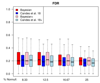
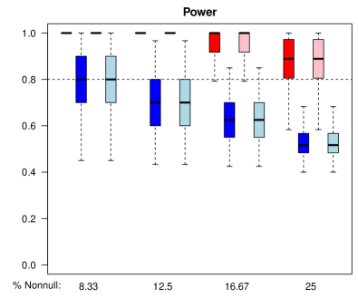
(a) Simulation results where latent covariates are independent

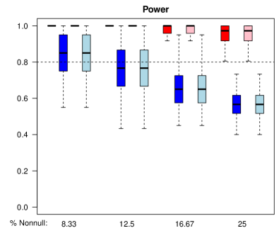
(b) Simulation results where latent covariates are generated from N($\mathbf{0}$,AR(0.5)) distribution

Figure 2: Comparison of Bayesian and Model-X knockoff generators for data with categorical covariates

In each simulation dataset, there are 200 observations with each containing $96$ continuous covariates and $48$ categorical covariates. Each categorical covariate has $5$ categories, which correspond to $4$ dummy variables. We consider 4 sparsity levels, where $1/4$ $(25\%)$, $1/6$ $(16.67\%)$, $1/8$ $(12.5\%)$ and $1/12$ $(8.33\%)$ of the features are not null. For sparsity level $r$, $96r$ coefficients for continuous covariates and $48r$ coefficients for categorical covariates are chosen to be non-zero. The signal strengths for nonnull features are randomly generated from either Unif$(1,2)$ or Unif$(3,5)$. For each scenario, we generate $200$ repeated datasets. We first generate $48+96$ continuous covariates from a $\mathrm{N}(\mathbf{0},\mathbf{I})$ or a N(0, AR(0.5)) distribution. For the latter, we permute the ordering of covariates. Then we convert the first $48$ covariates into categorical covariates through dividing the range of the original continuous covariates into intervals by quintiles and computing a categorical variable according to which interval its corresponding continuous variable occupies. The outcome and features are related through the linear model $Y=\mathbf{X}^{*}\boldsymbol{\beta}^{*}+\epsilon$, where $\mathbf{X}^{*}$ is the vector of nonnull features, $\boldsymbol{\beta}^{*}$ is the corresponding vector of non-zero coefficients, and $\epsilon$ is the noise with $\epsilon\sim\mathrm{N}(0,1)$. Both the Bayesian and the Gaussian Model-X knockoff use the group lasso penalty parameter for entering the model as the knockoff statistic, which is described in Section 2.2.

We summarize the empirical estimates of FDR for each scenario in the form of boxplots where covariate effects are in Unif$(1,2)$ in Figure 2. The red colors show the FDR and power of the Bayesian knockoff method, while the blue colors show the results of the Model-X knockoff. Light colors represent the knockoff$+$ filter, where an offset of $1$ is used in determining the threshold for feature selection. As expected, the FDR control is worse in situations where dummy covariates are simulated from AR(0.5) and knockoff$+$ filtering offers better FDR protection for both the Bayesian and the Gaussian Model-X methods. In Figure 2(a), the Bayesian knockoff procedures provide accurate FDR control, while their FDRs are mildly inflated in 2(b). For all sparsity levels, the Bayesian methods attain more than $80\%$ power on average while the Gaussian Model-X knockoff and knockoff+ filters have much lower power. The results for covariate effects in Unif$(3,5)$ are similar and are shown in the Supplemental Figure S1.

5.2 Knockoff Generators for Data from Mixture Distributions

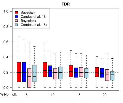
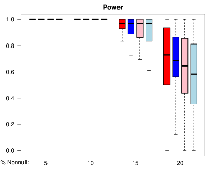
(a) Simulation results where covariates are generated from No$(\mathbf{0},\mathbf{I})$ distribution

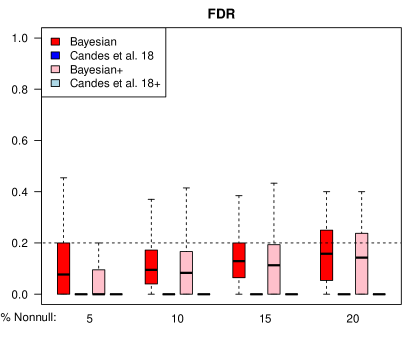
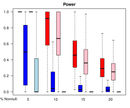
(b) Simulation results where covariates are generated from Normal mixture distribution

Figure 3: Comparison of Bayesian and Model-X knockoff generators for high dimensional continuous data

Datasets were simulated with 200 iid observations, each observation having one continuous outcome and 240 real-valued features. The outcome and features are related through the linear model $Y=\mathbf{X}^{*}\boldsymbol{\beta}^{*}+\epsilon$, where $\mathbf{X}^{*}$ is the vector of nonnull features and $\epsilon\sim\mathrm{No}(0,1)$. Four sparsity levels were considered: 5%, 10%, 15%, and 20%. Two choices of feature distribution and effects were evaluated: $\mathbf{X}\sim\mathrm{No}(\mathbf{0},\mathbf{I})$ and $\beta_{k}=3$ for nonnull features, and $\mathbf{X}\sim 0.5\cdot\mathrm{No}(\mathbf{1},\mathbf{I})+0.5\cdot\mathrm{No}(\mathbf{-1},\mathbf{I})$ (Normal mixture) and $\beta_{k}=12$ for nonnull features. For each configuration of simulation parameters, 200 replicate datasets were generated. The Gaussian DPM and Gaussian Model-X procedures were applied to generate knockoff features, followed by applying the knockoff filter for variable selection using the lasso signed max statistic in Equation (3).

Figure 3 summarizes these simulation results using boxplots of the empirical FDR and power estimates for each sparsity level and covariate distribution. Figure 3(a) considers the situation where the covariates have a normal distribution, as assumed by the Gaussian Model-X knockoff generator; in this case, both the Bayesian and Gaussian Model-X knockoff procedures provide FDR control near the targeted 20% level and offer similar power to detect true features. Figure 3(b), on the other hand, corresponds to the scenarios where covariates are simulated from a mixture of two normal distributions. Here, the Bayesian generators maintain FDR control near the targeted level, whereas the Gaussian Model-X generators fall far short of this level with interquartile ranges that are entirely collapsed upon 0%. The power attained by the Bayesian generators is superior as well, at 30-50% higher than the Gaussian Model-X procedures at each sparsity level. A substantial decrease in power is seen as the sparsity level increases under both feature distributions. Notably, the power also decreased greatly for each method when the features followed the normal mixture distribution compared to a standard normal distribution. For the sake of illustration, this necessitated the use of different signal strengths $\beta_{k}$ for the nonnull features under the standard normal and normal mixture distributions, with values of 3.0 used for the former and much larger values of 12.0 used for the latter. The reason for this sensitivity to the feature distribution is unclear, but may reflect underlying sensitivity of the lasso model to the feature distribution. Overall, the Bayesian generators are comparable to the Model-X methods in the case where the Gaussian Model-X’s assumptions hold while offering substantially better FDR control and higher power in situations where these assumptions are violated.

5.3 Knockoff Generators for Microbiome Data

In each simulation dataset, there are 200 observations and $240$ taxa features, with the counts of sequences summing to $10000$ in total for each observation. We first simulate latent log taxa abundance ratios (to the reference taxon) by generating a $200\times 239$ matrix, where each row is from a N($\mathbf{0}$, AR(0.1)) or a N($\mathbf{0}$, AR(0.5)). Then we permute the columns and take the exponential of this matrix. After that, we generate mean taxa abundance by adding a column of ones and rescaling the matrix by row so that each row sums to 1. The count sequence vector for each observation is generated from a multinomial distribution with the corresponding row of the standardized matrix as the probability vector.

Similar to the simulation setup of previous subsection, we consider 4 sparsity levels: $1/4$ $(25\%)$, $1/6$ $(16.67\%)$, $1/8$ $(12.5\%)$ and $1/12$ $(8.33\%)$. For sparsity level $r$, $120r-1$ coefficients are generated from Unif$(1,2)$, and $120r$ coefficients are generated from Unif$(-2,-1)$ for one set of simulations. To ensure that the coefficient sum to one constraint is satisfied, the first non-zero coefficient is then set equal to one minus the sum of the other coefficients. In a second set of simulations, we generate data where the true coefficients are from Unif$(3,5)$ and Unif$(-5,-3)$. The outcome and features are related through the linear model $Y=\mathbf{Z}^{*}\boldsymbol{\beta}^{*}+\epsilon$, where $\mathbf{Z}^{*}$ is the log relative abundance vector of nonnull features, $\boldsymbol{\beta}^{*}$ is the corresponding non-zero coefficients, which sum up to $0$, and $\epsilon$ is the noise term with $\epsilon\sim\mathrm{N}(0,1)$.

For each scenario, $200$ datasets were simulated. Both the Bayesian and Gaussian Model-X knockoff filters were applied to each dataset. Empirical estimates of the FDR and power are displayed in Figure 4 for the 8 scenarios, determined by 4 choices of sparsity levels and two choices of correlation structures among count probabilities. In terms of FDR control, the Gaussian Model-X knockoff+ performs the best, followed by the Bayesian knockoff+. In general, the Bayesian and the original methods are similar in terms of FDR performance; however, the Bayesian knockoff generator with modified lasso has better power in both scenarios. Except for the least sparse scenario, both the Bayesian knockoff and knockoff+ methods reach $80\%$ power on average. The Gaussian Model-X knockoff and knockoff+ methods fail to reach this level for any sparsity level considered. To summarize, the Bayesian knockoff$+$ gives the best performance by giving targeted FDR control without a big compromise in power. The simulation results with larger effect sizes are similar to the results with small effect sizes and are presented in the Supplemental Figure S2.

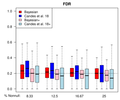
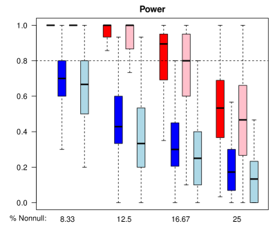
(a) Simulation results where latent covariates are generated from N($\mathbf{0}$,AR(0.1)) distribution

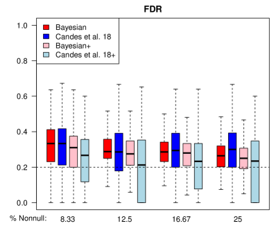
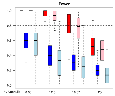
(b) Simulation results where latent covariates are generated from N($\mathbf{0}$,AR(0.5)) distribution

Figure 4: Comparison of Bayesian and Model-X knockoff generators for microbiome data

6 Real Data Examples

6.1 Predictors of Time to Alzheimer’s Disease in ANDI Dataset

We implemented the categorical Bayesian knockoff method on the Alzheimer’s Disease Neuroimaging Initiative (ADNI) dataset. Data used in the preparation of this article were obtained from the ADNI database (adni.loni.usc.edu). The ADNI was launched in 2003 as a public-private partnership, led by Principal Investigator Michael W. Weiner, MD. The primary goal of ADNI has been to test whether serial magnetic resonance imaging (MRI), positron emission tomography (PET), other biological markers, and clinical and neuropsychological assessment can be combined to measure the progression of mild cognitive impairment (MCI) and early Alzheimer’s disease (AD). There are 279 subjects in our analysis, and the outcome of interest is the time from mild cognitive impairment (MCI) to the diagnosis of Alzeimer’s disease (AD).

Candidate features include 11 baseline neuropsychological assessment indices; MRI volumetric data of ventricles, hippocampus, whole brain, entorhinal, fusiform gyrus, middle temporal gyrus, and intracerebral volume at the first visit; and single nucleotide polymorphisms (SNPs) that may have effects on the risk of developing AD. To reduce the number of SNPs, we follow the practice of Wu et al., (2020), who applied sure independent screening (Fan et al.,, 2010) and retained the top 500 SNPs. Here, baseline neuropsychological assessment indices and MRI volumetric data are continuous covariates, whereas for each SNP, homozygous without Thymine (coded 0), heterozygous or homozygous with Thymine (coded 1 and 2 separated) naturally form a categorical covariate with three categories.

Targeting an FDR of 20% and using the penalty parameter from a Cox lasso model as the importance statistic, our method selects 5 baseline assessment indices: the Alzheimer’s Disease Assessment Scale–Cognitive (ADAS 11), which assesses written and verbal responses of subjects; its modification, ADAS 13 (Kueper et al.,, 2018); the Rey Auditory Verbal Learning Test Immediate (RAVLT immediate), where a list of 15 words is read aloud to subjects across five consecutive trials, and then subjects are immediately asked to recall as many as words as they remember (Moradi et al.,, 2017); Functional Assessment Questionnaire (FAQ), which has 10 items with scores range from 0 to 30, with higher scores reflecting greater functional dependence) (Li et al.,, 2017); and the Digit Symbol Substitution Test score (DSST), where subjects are required to match symbols to numbers according to a key located on the top of the page), which is among the most commonly used tests in clinical neuropsychology. Among the selected assessment indices, ADAS 11, ADAS 13, RAVLT immediate, and FAQ were found to be the four strongest predictors of conversion to AD by Li et al., (2017).

Our knockoff filter also found baseline volume of hippocampus, entorhinal and middle temporal gyrus to be predictive of progression to AD. The entorhinal cortex and hippocampus are considered the first areas of the brain to be affected in Alzheimer’s disease (Khan et al.,, 2014; Dubois et al.,, 2016). Previous studies have suggested that atrophy of middle temporal gyrus in non-demented elderly predicts decline to AD (Visser et al.,, 2002; Convit et al.,, 2000). Our method identified 3 SNPs, rs1386236, rs1475950 and rs2428754 to be important predictors as well. Among them, rs1475950 and rs2428754 were also found to be important by Wu et al., (2020). SNP rs1386236 is part of the gene LUZP2, which controls the produce of leucine zipper protein 2. Leucine is found to play an important role in the development of AD and other metabolic disorders (Polis and Samson,, 2020). SNP rs1475950 is part of the GRM6 gene, which regulates glutamate. Wang and Reddy, (2017) pointed out that excessive excitatory glutamatergic neurotransmission causes excitotoxicity and promotes cell death, underlying a potential mechanism of neurodegeneration occurred in AD.

6.2 Gene Expression Predictors of Survival in Ovarian Cancer Patients

We evaluated the prognostic value of mRNA expression features for overall survival in ovarian cancer patients using The Cancer Genome Atlas (TCGA). Data were retrieved on 559 patients in the ovarian cancer cohort from TCGA, including 18632 gene expression features and times of death or last follow-up times for these patients. The expression features were log transformed and screened to retain only the most diverse features for selection; those features with log expression levels having a sample standard deviation greater than 0.16 were chosen for further evaluation. This produced a reduced set of 576 candidate features for knockoff selection.

Gene	Hazard ratio
CXCL13	$0.385$
B3GALT1	$1.742$
D4S234E	$0.342$
ZYG11A	$1.693$
LEMD1	$0.722$
OVGP1	$0.586$
CST9	$0.551$
UBD	$0.537$
NRG4	$0.331$
CCDC80	$2.708$
FLJ21963	$2.336$

Table 1: Estimated hazard ratios from reduced Cox model with selected genes from TCGA ovarian cancer dataset

To generate knockoff features for this set, we used both the GDPM model with recommended prior specified in Section 4 and the Gaussian Model-X procedure. The importance statistics used for knockoff selection were the signed max penalty parameters from a Cox lasso model of overall survival time, assuming random censoring. Knockoff filtering for both procedures was performed using the R package ”knockoff”. Table 1 displays the set of genes selected by the GDPM-based knockoff filter, along with estimated hazard ratios from a reduced Cox lasso model fitted using only the set of selected features. UBD, CXCL13, and D4S234E were also identified as having protective effects (estimated HR $<1$) on overall survival in a nine-gene panel constructed by Ding et al., (2020) from the TCGA database using a Cox lasso model. Gao et al., (2017) found OVGP1 to be protective with regard to overall survival in an analysis that found associations of 11 genes with survival using univariate log rank tests of each candidate gene. Because differing screening methods and/or analysis methods were used in each study to obtain its final panel of genes, we did not expect strong agreement between our set of selected genes and theirs. But, it is reassuring that some genes are shared across panels with estimated effects in the same direction.

6.3 Microbiome Features Predictive of BMI and CD14 Levels

We first illustrate our microbiome knockoff generator method without phylogeny tree information on a dataset that was used to investigate the association of dietary and environmental variables with the gut microbiota. Wu et al., (2011) collected stool samples from 98 healthy individuals and analyzed the sample DNA by 454/Roche pyrosequencing of 16S rDNA gene segments. Lin et al., (2014) also used this diet dataset as an illustrating example for their compositional lasso method, which we extended to calculate knockoff statistics for microbiome data.

There are 87 genera in this study and the outcome of interest is body mass index (BMI). The genera selected by our method are Clostridium, Oscillibacter, Acidaminococcus, and Allisonella, with the knockoff filter applied at a nominal FDR level of 20%. All of them are coming from the order Clostridiales. The genera Clostridium, Acidaminococcus, and Allisonella were also selected in Lin et al., (2014)’s paper. We then fit a reduced linear regression model with the log relative abundance of the four selected genera and the constraint that all coeffecients will sum up to $0$. The results are shown in Table 2. The effect sizes from the reduced linear regression model are comparable with the estimates from Lin et al., (2014)’s result using cross-validation.

Genus	Effect size for log abundance
Clostridium	$-1.075$
Oscillibacter	$-0.749$
Acidaminococcus	$0.748$
Allisonella	$1.076$

Table 2: Coefficients of the reduced compositional linear regression model with selected genera from Wu’s dataset

As an example of incorporating the phylogenentic structure into microbiome feature selection, we examine the HIV dataset from Bien et al., (2021). The outcome of interest is soluble CD14 levels in units of pg/ml, which has been identified as a mortality predictor in HIV infection. This fecal 16S rRNA amplicon dataset contains 152 observations with 539 OTUs per record and 87 phylogeny units from kingdom to genus level, i.e., 87 internal nodes in the phylogenetic tree. Targeting an FDR of $20\%$, twelve OTUs were selected by our procedure, one from phylum Firmicutes, family Lachnospiraceae; seven from phylum Actinobacteria, family Coriobacteriaceae; and four from phylum Actinobacteria, family Bifidobacteriaceae. Phylum Actinobacteria and family Lachnospiraceae were also detected in the original paper using cross validation. The effect sizes of relevant OTUs are listed in Table 3.

Phylum	Family	OTU	Effect size for log abundance
Firmicutes	Lachnospiraceae	$000518$	$0.564$
Actinobacteria	Coriobacteriaceae	$000357$	$0.074$
Actinobacteria	Coriobacteriaceae	$000230$	$-0.157$
Actinobacteria	Coriobacteriaceae	$000597$	$-0.011$
Actinobacteria	Coriobacteriaceae	$000404$	$0.004$
Actinobacteria	Coriobacteriaceae	$000500$	$-0.182$
Actinobacteria	Coriobacteriaceae	$000361$	$-0.039$
Actinobacteria	Coriobacteriaceae	$000378$	$0.006$
Actinobacteria	Bifidobacteriaceae	$000207$	$-0.009$
Actinobacteria	Bifidobacteriaceae	$000646$	$-0.008$
Actinobacteria	Bifidobacteriaceae	$000385$	$-0.150$
Actinobacteria	Bifidobacteriaceae	$000098$	$-0.092$

Table 3: Coefficients of the reduced compositional linear regression model with selected OTUs from Bien’s dataset

7 Discussion

This article proposes generating knockoff counterparts using parametric Bayesian models for datasets with categorical and/or continuous predictors and with microbiome features. Moreover, a Dirichlet process mixture model is proposed for continuously-valued feature vectors that provides additional flexibility for modeling feature distributions that may possess a complex structure, avoiding restrictive distributional assumptions. These methods are shown to identify important features with good FDR control and high power through simulations and real data applications. We recommend readers to extend the models presented in this paper and adopt Bayesian methods to generate knockoff copies as a routine practice.

One potential advantage of this Bayesian approach to knockoff construction is the incorporation of prior information about the feature space. This paper proposed using weak priors as a default choice when little is known about the feature distribution; simulations support the accuracy of our Bayesian knockoff generators with these priors. But, substantive knowledge may exist about the distribution of some or all candidate features a priori even though their relationship to the outcome is poorly understood. An informative prior can utilize this knowledge and potentially provide Bayesian knockoffs with closer structural resemblance to the true feature distribution, thereby improving the FDR control and power beyond that seen with a weak prior. This is an area worthy of further investigation.

Our methods focus upon improving the quality of knockoff generation for complex data contexts. This type of refinement and extension of existing knockoff generators has been the primary focus on new methodologic developments for knockoff filtering. Another component that has gained much less attention is the choice of importance statistic for filtering. The most common choices involve a lasso model and use either the lasso signed max (LSM) statistic or the lasso coefficient difference (LCD), the difference $|\hat{\beta}_{j}|-|\hat{\beta}_{j+p}|$ in sizes of coefficient estimates for the original and knockoff features. Candes et al., (2018) found that the LCD statistic tended to provide higher power than the LSM choice in most cases. Moreover, they suggest considering Bayesian models as importance statistics using the coefficient difference and note that the inclusion of accurate prior information in such models can boost the power over the LCD. We plan to study the use of Bayesian importance statistics in conjunction with our Bayesian knockoff generators to enhance the performance of these methods.

Though we rely on MCMC to simulate knockoff copies in this paper, other posterior inference methods, such as variational inference, should also be considered. This may be especially valuable when the dimension is high and exact inference is computationally expensive. In addition, the effect sizes obtained from reduced models with features selected by knockoff filters may be biased for the true effect sizes. Statistical methods are needed for determining accurate point and interval estimates for the effects of discovered features following a knockoff selection procedure. Post selection inference for knockoff filtering is an area that we want to explore in the future.

References

- Barber and Candès, (2015) Barber, R. F. and Candès, E. J. (2015). Controlling the false discovery rate via knockoffs. The Annals of Statistics, 43(5):2055–2085.
- Benjamini and Hochberg, (1995) Benjamini, Y. and Hochberg, Y. (1995). Controlling the false discovery rate: A practical and powerful approach to multiple testing. Journal of the Royal Statistical Society. Series B (Methodological), 57(1):289–300.
- Bien et al., (2021) Bien, J., Yan, X., Simpson, L., and Müller, C. L. (2021). Tree-aggregated predictive modeling of microbiome data. Scientific Reports, 11(1):14505.
- Candes et al., (2018) Candes, E., Fan, Y., Janson, L., and Lv, J. (2018). Panning for gold:‘Model-X’knockoffs for high dimensional controlled variable selection. Journal of the Royal Statistical Society: Series B (Statistical Methodology), 80(3):551–577.
- Chandra et al., (2020) Chandra, N. K., Canale, A., and Dunson, D. B. (2020). Escaping the curse of dimensionality in Bayesian model based clustering. arXiv preprint arXiv:2006.02700.
- Convit et al., (2000) Convit, A., de Asis, J., de Leon, M., Tarshish, C., De Santi, S., and Rusinek, H. (2000). Atrophy of the medial occipitotemporal, inferior, and middle temporal gyri in non-demented elderly predict decline to Alzheimer’s disease. Neurobiology of Aging, 21(1):19–26.
- Dai and Barber, (2016) Dai, R. and Barber, R. F. (2016). The knockoff filter for FDR control in group-sparse and multitask regression. arXiv preprint arXiv:1602.03589.
- Ding et al., (2020) Ding, Q., Dong, S., Wang, R., Zhang, K., Wang, H., Zhou, X., Wang, J., Wong, K., Long, Y., Zhu, S., Wang, W., Ren, H., and Zeng, Y. (2020). A nine-gene signature related to tumor microenvironment predicts overall survival with ovarian cancer. Aging, 12(6):4879.
- Dubois et al., (2016) Dubois, B., Hampel, H., Feldman, H. H., Scheltens, P., Aisen, P., Andrieu, S., Bakardjian, H., Benali, H., Bertram, L., Blennow, K., Broich, K., Cavedo, E., Crutch, S., Dartigues, J.-F., Duyckaerts, C., Epelbaum, S., Frisoni, G. B., Gauthier, S., Genthon, R., Gouw, A. A., Habert, M.-O., Holtzman, D. M., Kivipelto, M., Lista, S., Molinuevo, J.-L., O’Bryant, S. E., Rabinovici, G. D., Rowe, C., Salloway, S., Schneider, L. S., Sperling, R., Teichmann, M., Carrillo, M. C., Cummings, J., and Jack Jr, C. R. (2016). Preclinical Alzheimer’s disease: Definition, natural history, and diagnostic criteria. Alzheimer’s & Dementia, 12(3):292–323.
- Fan et al., (2010) Fan, J., Feng, Y., and Wu, Y. (2010). High-Dimensional Variable Selection for Cox’s Proportional Hazards Model, volume 6. Institute of Mathematical Statistics.
- Gao et al., (2017) Gao, Y., Liu, X., Li, T., Wei, L., Yang, A., Lu, Y., Zhang, J., Li, L., Wang, S., and Yin, F. (2017). Cross-validation of genes potentially associated with overall survival and drug resistance in ovarian cancer. Oncology Reports, 37(5):3084–3092.
- Gimenez et al., (2019) Gimenez, J. R., Ghorbani, A., and Zou, J. (2019). Knockoffs for the mass: new feature importance statistics with false discovery guarantees. arXiv preprint arXiv:1807.06214.
- Khan et al., (2014) Khan, U. A., Liu, L., Provenzano, F. A., Berman, D. E., Profaci, C. P., Sloan, R., Mayeux, R., Duff, K. E., and Small, S. A. (2014). Molecular drivers and cortical spread of lateral entorhinal cortex dysfunction in preclinical Alzheimer’s disease. Nature Neuroscience, 17(2):304–311.
- Kueper et al., (2018) Kueper, J. K., Speechley, M., and Montero-Odasso, M. (2018). The Alzheimer’s Disease Assessment Scale–cognitive subscale (adas-cog): Modifications and responsiveness in pre-dementia populations. A narrative review. Journal of Alzheimer’s Disease, 63:423–444. 2.
- Li et al., (2017) Li, K., Chan, W., Doody, R. S., Quinn, J., Luo, S., and the Alzheimer’s Disease Neuroimaging Initiative (2017). Prediction of conversion to Alzheimer’s disease with longitudinal measures and time-to-event data. Journal of Alzheimer’s Disease, 58:361–371. 2.
- Lin et al., (2014) Lin, W., Shi, P., Feng, R., and Li, H. (2014). Variable selection in regression with compositional covariates. Biometrika, 101(4):785–797.
- Lo, (1984) Lo, A. Y. (1984). On a Class of Bayesian Nonparametric Estimates: I. Density Estimates. The Annals of Statistics, 12(1):351 – 357.
- Moradi et al., (2017) Moradi, E., Hallikainen, I., Hänninen, T., and Tohka, J. (2017). Rey’s Auditory Verbal Learning Test scores can be predicted from whole brain MRI in Alzheimer’s disease. NeuroImage: Clinical, 13:415–427.
- Neal, (2000) Neal, R. M. (2000). Markov chain sampling methods for Dirichlet process mixture models. Journal of Computational and Graphical Statistics, 9(2):249–265.
- Polis and Samson, (2020) Polis, B. and Samson, A. (2020). Role of the metabolism of branched-chain amino acids in the development of Alzheimer’s disease and other metabolic disorders. Neural Regeneration Research, 15(8):1460–1470.
- Shi et al., (2019) Shi, Y., Martens, M., Banerjee, A., and Laud, P. (2019). Low information omnibus (LIO) priors for Dirichlet process mixture models. Bayesian Analysis, 14(3):677–702.
- Simpson et al., (2021) Simpson, L., Combettes, P. L., and Müller, C. L. (2021). c-lasso - a python package for constrained sparse and robust regression and classification. Journal of Open Source Software, 6(57):2844.
- Srinivasan et al., (2020) Srinivasan, A., Xue, L., and Zhan, X. (2020). Compositional knockoff filter for high-dimensional regression analysis of microbiome data. Biometrics, n/a(n/a).
- Tibshirani, (1996) Tibshirani, R. (1996). Regression shrinkage and selection via the lasso. Journal of the Royal Statistical Society: Series B (Methodological), 58(1):267–288.
- Vannucci, (2020) Vannucci, M. (2020). Edge-selection priors for graphs estimation with applications to complex data. Joint Statistical Meeting (JSM) Presentation.
- Visser et al., (2002) Visser, P. J., Verhey, F. R. J., Hofman, P. A. M., Scheltens, P., and Jolles, J. (2002). Medial temporal lobe atrophy predicts Alzheimer’s disease in patients with minor cognitive impairment. Journal of Neurology, Neurosurgery & Psychiatry, 72(4):491–497.
- Wang and Reddy, (2017) Wang, R. and Reddy, P. H. (2017). Role of glutamate and NMDA receptors in Alzheimer’s disease. Journal of Alzheimer’s Disease, 57:1041–1048. 4.
- Wu et al., (2011) Wu, G. D., Chen, J., Hoffmann, C., Bittinger, K., Chen, Y.-Y., Keilbaugh, S. A., Bewtra, M., Knights, D., Walters, W. A., Knight, R., Sinha, R., Gilroy, E., Gupta, K., Baldassano, R., Nessel, L., Li, H., Bushman, F. D., and Lewis, J. D. (2011). Linking long-term dietary patterns with gut microbial enterotypes. Science, 334(6052):105–108.
- Wu et al., (2020) Wu, Q., Zhao, H., Zhu, L., and Sun, J. (2020). Variable selection for high-dimensional partly linear additive Cox model with application to Alzheimer’s disease. Statistics in Medicine, 39(23):3120–3134.
- Yuan and Lin, (2006) Yuan, M. and Lin, Y. (2006). Model selection and estimation in regression with grouped variables. Journal of the Royal Statistical Society: Series B (Statistical Methodology), 68(1):49–67.