Alleviating the transit timing variation bias in transit surveys

Transit timing variations (TTVs) can provide useful information for systems observed by transit, as they allow us to put constraints on the masses and eccentricities of the observed planets, or even to constrain the existence of non-transiting companions. However, TTVs can also act as a detection bias that can prevent the detection of small planets in transit surveys that would otherwise be detected by standard algorithms such as the Boxed Least Square algorithm (BLS) if their orbit was not perturbed. This bias is especially present for surveys with a long baseline, such as Kepler, some of the TESS sectors, and the upcoming PLATO mission. Here we introduce a detection method that is robust to large TTVs, and illustrate its use by recovering and confirming a pair of resonant super-Earths with ten-hour TTVs around Kepler-1705 (prev. KOI-4772). The method is based on a neural network trained to recover the tracks of low-signal-to-noise-ratio(S/N) perturbed planets in river diagrams. We recover the transit parameters of these candidates by fitting the light curve. The individual transit S/N of Kepler-1705b and c are about three times lower than all the previously known planets with TTVs of 3 hours or more, pushing the boundaries in the recovery of these small, dynamically active planets. Recovering this type of object is essential for obtaining a complete picture of the observed planetary systems, and solving for a bias not often taken into account in statistical studies of exoplanet populations. In addition, TTVs are a means of obtaining mass estimates which can be essential for studying the internal structure of planets discovered by transit surveys. Finally, we show that due to the strong orbital perturbations, it is possible that the spin of the outer resonant planet of Kepler-1705 is trapped in a sub- or super-synchronous spin–orbit resonance. This would have important consequences for the climate of the planet because a non-synchronous spin implies that the flux of the star is spread over the whole planetary surface.

1 Introduction

The most successful technique for detecting exoplanets —in terms of number of planets detected— is the transit method: when a planet passes in front of a star, the flux received from that star decreases. This technique has been, is being, and will be applied by several space missions such as CoRoT, Kepler/K2, TESS, and the upcoming PLATO mission, to try and detect planets in large areas of the sky. When a single planet orbits a single star, its orbit is periodic, which implies that the transit happens at a fixed time interval. This constraint is used to detect planets when their individual transits are too faint with respect to the noise of the data: using algorithms such as Boxed Least Squares (BLS, Kovács et al., 2002), the data-reduction pipelines of the transit survey missions fold each light curve over a large number of different periods and look for transits in the folded data (Jenkins et al., 2010, 2016). This folding of the light curve increases the number of observations per phase, and therefore improves the signal-to-noise ratio (S/N) of any transit.

As soon as two or more planets orbit around the same star, their orbits cease to be strictly periodic. In some cases the gravitational interaction of planets can generate relatively short-term transit timing variations (TTVs): transits no longer occur at a fixed period (Dobrovolskis & Borucki, 1996; Agol et al., 2005). The amplitude, frequency, and overall shape of these TTVs depend on the orbital parameters and masses of the planets involved (see e.g. Lithwick et al., 2012; Nesvorný & Vokrouhlický, 2014; Agol & Deck, 2016). As the planet–planet interactions that generate the TTVs typically occur on timescales longer than the orbital periods, space missions with longer baselines such as Kepler and PLATO are more likely to observe such effects. Since the end of the Kepler mission, several efforts have been made to estimate the TTVs of the Kepler Objects of Interest (KOIs) (Mazeh et al., 2013; Rowe & Thompson, 2015; Holczer et al., 2016; Kane et al., 2019).

Transit timing variations are a goldmine for our understanding of planetary systems: they can be used to constrain the existence of non-transiting planets, thereby adding missing pieces to the architecture of the systems (Xie et al., 2014; Zhu et al., 2018), and allowing for a better comparison with synthetic planetary system population synthesis models (see e.g. Mordasini et al., 2009; Alibert et al., 2013; Mordasini, 2018; Coleman et al., 2019; Emsenhuber et al., 2020). TTVs can also be used to constrain the masses of the planets involved (see e.g. Nesvorný et al., 2013), and therefore their density, which ultimately provide constraints on their internal structures, as is the case for the Trappist-1 system (Grimm et al., 2018; Agol et al., 2020). Detection of individual dynamically active systems also provides valuable constraints on planetary system formation theory, as the current orbital state of a system can display markers of its evolution (see e.g. Batygin & Morbidelli, 2013; Delisle, 2017). Orbital interactions also impact the possible rotation state of the planets (Delisle et al., 2017), and therefore their atmosphere (Leconte et al., 2015).

However, TTVs can also prevent the detection of exoplanets. As previously stated, transit surveys rely on stacking the light curve over a constant period to extract the shallow transits from the noise. If TTVs of amplitude comparable to or greater than the duration of the transit occur on a timescale comparable to or shorter than the mission duration, there is not a unique period that will successfully stack the transits of the planet (García-Melendo & López-Morales, 2011). This can lead to two problems: incorrect estimates of the planet parameters, and/or the absence of detection. In particular, Kane et al. (2019) identified that the lack of known small planets with large TTVs is consistent with an observational bias. In recent years, approaches have been developed to recover the correct transit parameters of known planets exhibiting TTVs, such as for example the photo-dynamical model of the light curve Ragozzine & Holman (2010), or the spectral approach by Ofir et al. (2018). However, these approaches require detection of the planets. The QATS algorithm alleviates part of this bias (Carter & Agol, 2013; Kruse et al., 2019), relaxing the strict periodic constraint of other detection algorithms such as the BLS, by allowing the duration between transits to vary within a given range. This gives the algorithm the clear advantage of being able to correct for any TTV shape within a given range of instantaneous periods, but it also leads to a decrease in efficiency for larger TTVs and smaller S/Ns of individual transits, as the stochastic background increases with the range of allowed instantaneous periods.

In recent years, neural networks have been used to vet planetary transits and other astronomical phenomena, or even to detect new planets (see e.g. Shallue & Vanderburg, 2018; Pearson et al., 2018; Osborn et al., 2020; Armstrong et al., 2020), with approaches that were based on the study of individual transits. In this paper, we present a transit detection method that is adapted to low-S/N planets —i.e. with individual transits that are shallower than the standard deviation of the photometric flux— and is robust to TTVs. To do so, we formulate the problem with an image-recognition approach (Krizhevsky et al., 2012).

The paper is structured as follows: in section 2 we discuss the problem of TTV bias. In Section 3 we introduce the RIVERS (recognition of interval variations in exoplanet recovery surveys) method using Kepler-36b as an example. In section 4, we use the RIVERS method to detect and characterise a pair of resonant planets around Kepler-1705. The dynamics of the resonant pair is discussed in section 5. Finally, we discuss the choices and caveats of the method, and conclude in section 6.

2 The problem

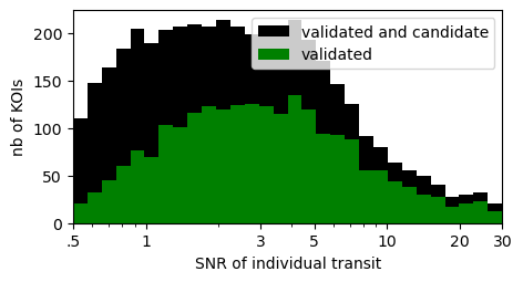
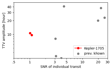
Figure 1: Top: Individual transit S/N for all validated KOIs (Exoplanet Archive Disposition of ‘confirmed’) or candidate (disposition of ‘candidate’) as of May 2021. Bottom: Peak-to-peak TTV amplitude of Kepler planets and candidates as a function of the S/N of individual transits, for planets with TTVs of more than 3 hours of peak-to-peak amplitude. Previously known systems include: Kepler-30 (Panichi et al., 2018), Kepler-88 (Nesvorný et al., 2013), KOI-227 (Nesvorný et al., 2014), Kepler-223 (Mills et al., 2016), Kepler-603 (Holczer et al., 2016), and Kepler-36 (Carter et al., 2012).

As mentioned in Sect. 1, the data-reduction pipeline of the transit survey missions such as Kepler/K2 and TESS (Jenkins et al., 2010, 2016) uses the BLS algorithm (Kovács et al., 2002), which folds each light curve over a large range of different periods and looks for transits in these folded data.

For a dataset with a flux $f$ associated with the time $t$, folding over the period $P$ is equivalent to mapping $f$ to $\varphi=\text{mod}(t,P)$. Folding the light curve therefore increases on average the number of measurements per bin of phase $\varphi$ of the chosen period $P$ by a factor $N$, where $N$ is the number of times the light curve was folded. As a result, the S/N of the transits of the planet in the folded light curve is increased by a factor $\sqrt{N}$ compared to the individual transits in the unfolded light curve.

In multi-planetary systems, planet–planet interaction can generate TTVs (Dobrovolskis & Borucki, 1996; Agol et al., 2005). In particular, planets near or in mean motion resonance (MMR) can exhibit significant TTV over a timescale comparable to or smaller than the baseline of transit surveys such as Kepler and PLATO. The typical timescale of these configurations and their dependence on the planetary masses and eccentricities are given in Appendix A.

We define S/N_i as the S/N of an individual transit of a planet:

$$\text{S/N}_{i}=\sqrt{N_{\text{transit}}}D/\sigma_{lc}\,,$$ (1)

where $D$ is the depth of the transit, $N_{\text{transit}}$ is the number of measurements during one transit and $\sigma_{lc}$ is the standard deviation of the flux of the light curve. When these configurations induce TTVs that have a period comparable to or shorter than the duration of the data and a peak-to-peak amplitude $\sigma_{TTV}$ comparable to or larger than the transit duration $T_{transit}$ of the planet, the smearing of the folded transit leads to alteration of the determined transit parameters. In addition, the S/N of the transit is reduced, which can prevent the detection of the planet. Assuming the TTVs are sinusoidal and the transit is box-shaped, for observations longer than the TTV period the depth of the stacked transit can be estimated by (see Appendix B):

$$\text{Smeared Depth}=D/(1+\sigma_{TTV}/T_{transit})\,.$$ (2)

We can therefore estimate the smeared S/N of a planet using the following formula:

$$\text{Smeared S/N}=\frac{\text{S/N}_{i}}{1+\sigma_{TTV}/T_{transit}}\sqrt{\frac{\text{Mission duration}}{\text{Orbital period}}}.$$ (3)

In the Kepler mission, if the smeared S/N is below 7.1, the signal will not be considered as a KOI. This is probably why all known Kepler planets with a large TTV also have a large S/N_i. The top part of Fig. 1 shows the S/N_i of all KOIs. The bottom part shows the known planets with a peak-to-peak TTV of greater than 3 hours and a S/N_i below 30. All of these planets have a S/N_i above 3, which allowed either their detection in a stacked light curve despite the smearing of the transit or the detection of their individual transits. The comparison of the two figures shows an over-representation of planets with large S/N_i in the population of planets with large TTVs. If anything, the underlying expected trend is the opposite: for a pair of planets in or near mean-motion resonance, the relative amplitude of TTVs between the two planets is proportional to $TTV_{1}/TTV_{2}\propto m_{2}/m_{1}$, yielding larger TTVs for the least massive planet of the pair. In addition, in the co-orbital resonance, the lower the sum of the masses of the two planets, the larger the TTV amplitude can be (Leleu et al., 2019). We therefore expect a subpopulation of planets with large TTVs and small S/N_i that is currently missed in transit surveys because of the TTV bias.

3 RIVERS approach

We aim to alleviate the bias that prevents standard algorithms from recovering and characterising the small, dynamically active planets that could have been missed in transit surveys. To do so, we need to recover in a given light curve a large number of transits that are individually too small to be identified. We therefore skip the determination of individual transits and focus on the fit of the light curve by transit models whose timing is constrained using TTV models. The model ensures that the TTVs follow a signal that is physically possible, reducing the space of available TTVs compared to an approach in which each transit timing is freely fitted to the data. This approach also reduces the number of free parameters to a maximum of five per planet for a coplanar system, against one free parameter per transit. The downside is that the method will only be able to identify planets whose TTVs are dominated by the effect of the planets that are considered in the model. The TTVs can be modelled by N-body simulations, allowing for an accurate TTV prediction regardless of the number of modelled planets and orbital configuration (see e.g. Deck et al., 2014). In the case of two interacting planets, analytical models can be used for specific configurations; see for example Agol & Deck (2016) and Deck & Agol (2016) for the TTVs of a pair of planets outside of MMR, and Nesvorný & Vokrouhlický (2016) for the TTVs of a pair of planets in first-order MMR. The analytical approach can be up to two orders of magnitude faster (Deck & Agol, 2016) and further reduce the number of free parameters.

This approach uses TTV modelling as a means of detection in addition to a tool for the characterisation of the system. However, these fits are too time consuming to be applied to all Kepler stars for any orbital period. We therefore need an algorithm to identify promising orbital periods for a given star which does not rely on the exact periodicity between the transits to detect candidates. We base our approach on shape recognition in a 2D representation of the light curve called a river diagram (or riverplot, introduced by Carter et al., 2012). We illustrate this method in the following section using the well-known example of Kepler-36b.

3.1 Kepler-36b

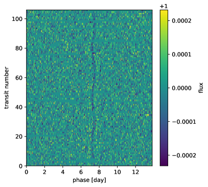
Figure 2: River diagram of Kepler-36 at the period 13.848d: the bottom row displays the first 13.848 days of data for Kepler-36, with the colour code representing the normalised flux. Each subsequent row displays a new set of 13.848 days of data. The flux has been clipped at $3\sigma$ for visibility, and missing data have been replaced by a flux of 1.

Kepler-36b has a TTV amplitude of about 8 hours for a transit duration of 7 hours (Carter et al., 2012). The river diagram of the DPCSAP flux of Kepler-36 for $P_{\text{fold}}=13.8480\,$days is shown in Fig. 2. In a river diagram, each line displays the normalised flux coming from the star over a single (constant) orbital period $P_{\text{fold}}$. When $P_{\text{fold}}$ is close to the average orbital period of a planet or its aliases, subsequent transits of the planets vertically align, allowing the eye to track the signature of the planet. A planet without TTVs produces a straight line, while TTVs induce variations in the horizontal position of each transit. If $P_{\text{fold}}\approx P_{\text{orb}}$, a single curve appears. If $P_{\text{fold}}\approx kP_{\text{orb}}$, with $k$ an integer, $k$ full curves appear in the diagram. More generally, if $jP_{\text{fold}}\approx kP_{\text{orb}}$ with $k$ and $j$ being positive integers, $k$ curves appear, with a transit every $j$ lines.

The track of Kepler-36b, with an S/N_i of $3.07$, is clearly visible in the river diagram. The S/N_i is sufficient to recover the planet in the BLS despite the smearing: the top panel of Fig. 3 shows the BLS periodogram applied to the the pre-search data-conditioning simple aperture photometry (PDCSAP) flux of Kepler-36, once the transits of Kepler-36c (16.23d) are masked. An analysis of the light curve using the QATS algorithm was able to recover the individual transits, leading to characterisation of the resonant pair Kepler-36b and Kepler-36c (Carter et al., 2012).

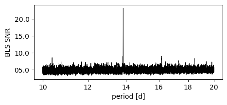
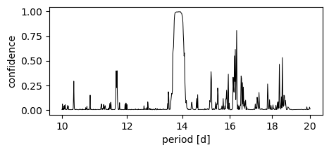
Figure 3: Periodograms of the PDCSAP flux of Kepler-36, once the transits of Kepler-36c (16.23d) are masked. Top: BLS periodogram. Bottom: RIVERS periodogram. The y axis represents the confidence in the model that the river diagram folded at the period shown on the x-axis has a planet-like track.

3.2 The RIVERS.deep approach

3.2.1 Model architecture

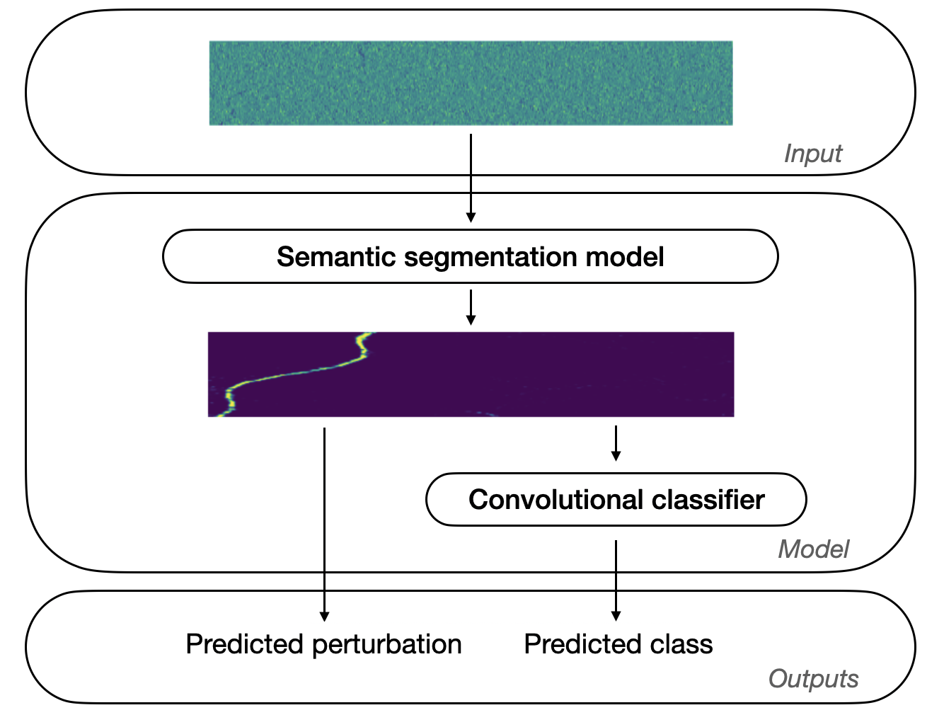
Figure 4: Neural network model architecture. The model takes a river diagram as input, computes a predictions mask, and feeds it into a convolutional neural network (CNN) classifier. The model output is the couple (predicted mask, CNN prediction).

As long as $P_{\text{fold}}$ is close enough to the average orbital period of the planet, river diagrams are a 2D representation of the light curve in which the track of a planet draws a curve. As neural networks have been shown to be well suited to performing pattern recognition (Krizhevsky et al., 2012), we developed the RIVERS.deep algorithm, which takes as input a river diagram such as that shown in Fig. 2 and produces two outputs:

• A confidence matrix: An array of the same size as the input containing for each pixel the confidence that this pixel belongs to a transit. This task is performed by the ‘semantic segmentation’ (pixel-level vetting) subnetwork (Jégou et al., 2017).

• global prediction: A value between 0 and 1 which quantifies the model confidence that the output of the semantic segmentation module is due to the presence of a planet. This task is performed by the classification subnetwork.

Our model works with arrays of fixed size, while the sizes of river diagrams depend on the duration of the dataset and $P_{\text{fold}}$ for a fixed bin size (taken at $30\,$min for this study). The river diagrams are therefore all resized to a given size using the nearest interpolation method, which gave the best results amongst the methods tested (bilinear interpolation, nearest, padding the missing pixels with values of 1, and a mosaic repetition of the river diagram). To avoid losing information, the number of pixels along the x-axis is determined by the longest considered period divided by the bin size, while the y-axis is set by the duration of the observations divided by the shortest considered period. To avoid too much stretching of the matrices, we trained different models for different period ranges: 5 to 10 days, 10 to 20 days, and 20 to 30 days. The global architecture of the model is illustrated in Fig. 4 and a precise description of the components is available in Appendix C. Several architecture experiments are also discussed in that Appendix.

3.2.2 Training set

In order to train the neural network, we generated a large set of inputs (river diagrams), and their expected outputs: a transit mask and a boolean indicating the presence of a planet with a mean period close to the folded period. Transit masks are arrays of the same shape as the river diagram. If the river diagram contains the track of a planet, the transit mask contains ‘1’ in transits and ‘0’ everywhere else. When the river diagram does not contain a planet, the transit mask is full of zeros. For best performance of the model, the training dataset has to be as close as possible to the real data; it is therefore preferable to train a model dedicated to a given mission. In this paper, we focus on the Kepler light curves as their duration allows us to use exploit the full potential of our method with its 4 years of continuous observation. Ideally, we would train our model on real planets. However there are not enough planets with large TTVs and low S/N to constitute a training set.

We therefore generated a synthetic training set of 40,000 river diagrams for each of the period ranges mentioned in the previous section. To do so, we generated a set of 40,000 unique orbital configurations: to train a model to recognise planets with periods in the range of 10 to 20 days, the period of the transiting planet $P_{1}$ is randomly chosen between $10.2$ and $19.8\,$d with a flat probability. The (neighbouring) MMR is then randomly picked amongst $k:k+1$ or $k+1:k$ for $1\leq k\leq 8$, $k:k+2$ or $k+2:k$ for $k=\{1,3,5\}$, or the $1:1$ MMR. The initial period of the non-transiting planet is taken at the exact resonance multiplied by $1+3\theta\sqrt{(m_{1}+m_{2})/m_{\star}}$, where $\theta$ is randomly chosen between $-0.5$ and $0.5$. The eccentricities are chosen randomly between $0$ and $0.1$, and all angles are randomised. The systems were integrated as coplanar, although only planet 1 is injected in the light curve, which should not significantly impact the results, as analytical studies point out that small mutual inclinations do not impact the shapes of TTVs (Nesvorný & Vokrouhlický, 2016). Only systems that were short-term unstable (collision or ejection from the initialised configuration over the 10 years of integration) were removed from this dataset.

Each of these 40,000 orbital solutions is then injected in one of the selected Kepler light curve. The light curves were selected through the kplr package, with the following filters: The light curve has to contain at least one confirmed planet of period between 3 and 50 days, and no false​ positive or not​ dispositioned KOIs, regardless of their period. This resulted in about 1,200 unique light curves. For each light curve, the raw PDCSAP flux is downloaded using the lightkurve package. The signal of all known planets or KOIs is masked: data points falling in or near the transits are removed from the dataset. For planets with known TTVs, we removed an additional width of 1.5 times the TTV amplitude reported in Kane et al. (2019).

To inject the signal of the perturbed planet in a Kepler light curve, its effect on an ideal normalised light curve (noiseless) is computed at the date of each data point of the light curve using the batman package (Kreidberg, 2015). The parameters of the star, such as its radius and limb-darkening coefficients, are obtained through the kplr package. The raw PDCSAP flux and the idealised light curve are then multiplied data point by data point, simulating the transit of the injected planet. The obtained light curve is then detrended using the flatten method of the lightkurve package using the default parameters. This method applies a Savitzky-Golay filter to the light curve. The whole process results in a synthetic light curve containing the transits of a dynamically active planet, with noise structure identical to that particular Kepler target.

Finally, we split the light curves into two groups. With half of the synthetic light curves we generate a river diagram with $P_{fold}$ close enough to the average period $P$ of the injected planet so that the track of the planet appears only once per line in the diagram. For a planet without TTVs, this corresponds to a range of periods in which the track of the planet makes anything from a bottom-left to top-right diagonal of the river diagram, to a bottom-right to top-left diagonal, hence $P-\delta P<P_{fold}<P+\delta P$, where

$$\delta P=P^{2}/T\,,$$ (4)

where T is the mission duration. These are the river diagrams we label as goodfold and correspond to the presence of a planet for the classifier subnetwork. We do not train only on diagrams where $P_{fold}=P$ because $P$ is not known in advance when looking for new planets, and therefore the model needs to be able to recognise tilted planet tracks. The remaining halves of the light curves are used to generate river diagrams with a random period in the range of 10 to 20 days, excluding periods that correspond to $P-2\delta P<P_{fold}<P+2\delta P$. We label those as badfold, corresponding to the absence of a planet at $P_{fold}$ for the classifier subnetwork.

3.2.3 Periodogram

In order to visualise whether or not a given star harbours promising candidates, we generate a periodogram of the light curve by creating river diagrams for a subset of $P_{fold}$ that span the range of periods for which the model was trained. As discussed in the previous section, we need to ensure that regardless of the period $P$ of the potential planet, there are river diagrams that will be evaluated at $P_{fold}$ such that $|P_{fold}-P|<\delta P$ (Eq. 4). As the recovery rate of the model is not $100\%$, we sample the period range with a smaller period step by introducing the parameter $N_{diag}$. Starting at $P_{0}$, which is the smallest period on which the model is trained, the set of periods $P_{n}$ that form the periodogram is defined recurrently, following:

$$P_{n}=P_{n-1}+\delta P_{n-1}/N_{diag}\,.$$ (5)

For each $P_{n}$, the periodogram shows the confidence of the model that the river diagram contains the track of a planet.

3.2.4 Application of the model

The bottom panel of Fig. 3 shows the RIVERS.deep periodogram applied on the PDCSAP flux of Kepler-36, once the transits of Kepler-36c (16.23d) are masked. A wide peak of confidence of approximately $1$ appears near $P_{\text{fold}}=13.8\,$days which is the average orbital period of Kepler-36b. The river diagram shown in Fig. 2 belongs to the peak of this periodogram. Figure 5 shows the confidence matrix corresponding to the same river diagram, where the semantic segmentation task highlighted the timings that belong to the transits. These timings can be used to estimate a proxy of transit timings that can then be used to perform a preliminary fit of the TTV model, ensuring that the subsequent fit of the light curve is initialised near the solution. In addition, stacking the light curve along the proxy of the transit timings allows us to approximate the transit parameters such as the planetary radii and impact parameter for the initialisation of the photodynamic fit. In the following section, we show how this approach allowed us to discover and confirm a pair of resonant planets around Kepler-1705.

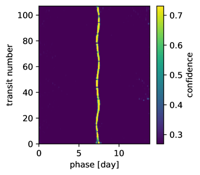
Figure 5: RIVERS.deep confidence matrix. Each pixel corresponds to the same bin of the light curve as the corresponding river diagram shown in Fig. 2. The colours show the confidence of the model that the timing belongs to the track of a planet.

4 Detection and study of Kepler-1705b and Kepler-1705c

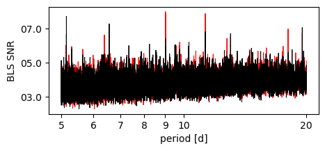
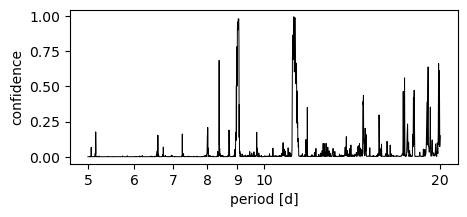
Figure 6: Periodogram of the light curve of Kepler-1705 after removal of the 3.08d candidate. Top: BLS periodogram on the first 12 quarters in red, on the full dataset in black. Bottom: RIVERS periodogram on the full dataset. The peaks around 9.03d and 11.3d have a non-zero width, implying that subsequent frames had a high confidence from the model. Examples of river diagrams for each of these peaks are given in Fig. 7.

Kepler-1705 (KOI4772, KIC 8397947) is an F star (6300K) with a magnitude of $mV=15.800\pm 0.206$, $m_{Kep}=15.514$. As of October 5, 2021, two candidates at 3.38 d (KOI4772.01) and 9.01 d (KOI4772.02) and a false positive at 39.09 d (KOI4772.03) are announced on the Kepler database. An analysis by the BLS algorithm of the flattened PDCSAP flux (section 3.2.2) of all available quarters allows KOI4772.01 to be recovered at the announced 3.38d period. However, once the transits of KOI4772.01 are masked, a second use of the BLS yields no significant peak in the range of 5 to 20 days; see the black periodogram in the top panel of Fig. 6.

4.1 Application of the RIVERS.deep method

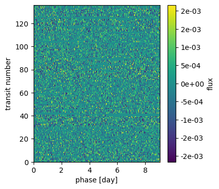
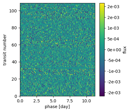
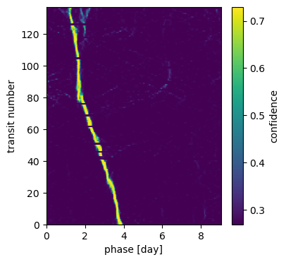
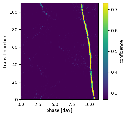
Figure 7: Top: River diagrams of Kepler-1705 at the period of 9.0471d (left) and 11.3059 (right). The bottom left corner starts at 352.3975 [BJD-2454833.0] for both. See Fig 2 for more details. Bottom: Corresponding RIVERS.deep confidence matrices, which shows the confidence for each timing of the rivers diagram to belong to the track of a planet. See section 3.2.1 for more details about the confidence matrix.

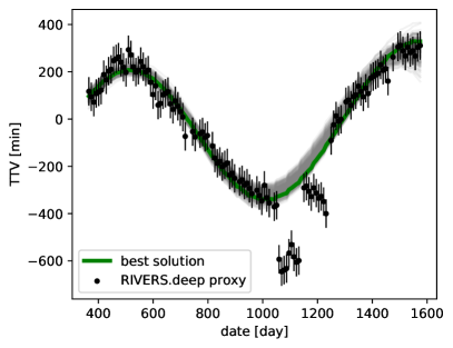
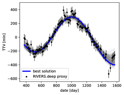
Figure 8: TTVs for Kepler-1705b (top) and Kepler-1705c (bottom). The black error bars represent the TTVs proxy coming from the RIVERS.deep method. The dates are in [BJD-2454833.0]. In grey are 300 samples resulting from the fit of the light curve. The solid coloured curves correspond to the best fit.

We further analysed the light curve using the approach explained in Section 3. The bottom panel of Fig. 6 shows the RIVERS periodogram applied on the same dataset as the black BLS periodogram shown in the top panel. In the RIVERS periodogram, two peaks appear at $\sim 9.0$ and $\sim 13.2$ days. The river diagram and RIVERS.deep matrix for a frame chosen in each of these peaks are shown in Fig. 7. For each of these periods, the model identified a coherent track for the entire duration of the Kepler mission. We then retrieved the proxy of transit timings from each of the RIVERS.deep diagrams of Fig. 7. The TTVs corresponding to these transit timings are shown with black circles in Fig. 8. We note that the error bars are simply an indication of the resolution of the river diagram (bins of 30 mins). The two signals appear to be in phase opposition, as expected for the TTVs of two strongly interacting planets. Indeed, the two peaks lie close to the 5:4 MMR. Although caveats of the method are discussed in section 6.1, we stress that these are not equivalent to transit timings that could have been fitted to the light curve, but the output of a neural network trained to recover the track of TTV-perturbed planets in river diagrams. The validation of the candidates comes from the fit of the light curve.

4.1.1 Comparison to the result of the BLS

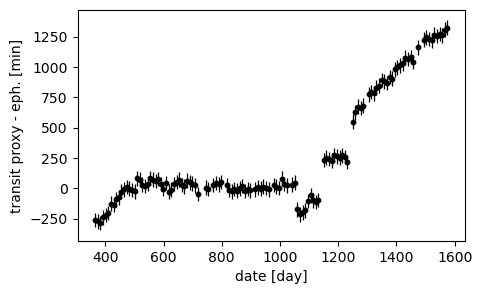
Figure 9: Difference between the RIVERS.deep transit proxy of the RIVERS candidate at $\sim 9$d (Kepler-1705b) and the ephemeride of KOI4772.02 from the exoplanet archive. The dates are in [BJD-2454833.0].

As shown in Fig. 9, the timings of the RIVERS candidate at $\sim 9$d (Kepler-1705b) are coherent with the KOI4772.02 candidate published on the exoplanet archive. In the first half of the data, a significant part of the transit timings can indeed be modelled by a straight line, which explains why KOI4772.02 is only found in the Q1-Q12 table of the exoplanet archive: the corresponding peaks appear in the BLS only when analysing the 1-12 quarters; see the red periodogram in the top panel of Fig. 6. On that periodogram, we can see that the 11.3d signal was also on the threshold to become a KOI. This demonstrates that in the BLS periodogram, a signal with TTV can appear with a higher S/N with less data because a locally constant period prevents the smearing of the stacked transit, as discussed in Section 2.

4.2 Planet detection

Table 1: Stellar properties of Kepler-1705

Kepler-1705
KIC	8397947
Parameter	Value	Note
mKep [mag]	15.514	1
mV [mag]	$15.800\pm 0.206$	1
mJ [mag]	$14.210\pm 0.029$	1
mH [mag]	$13.868\pm.031$	1
$T_{\mathrm{eff}}$ [K]	$6312_{-152}^{+215}$	2
$\log{g}$ [cgs]	$4.298_{-0.047}^{+0.043}$	2
[Fe/H] [dex]	$-0.20_{-0.15}^{+0.15}$	2
$R_{\star}$ [$R_{\odot}$]	$1.259_{-0.051}^{+0.032}$	2
$M_{\star}$ [$M_{\odot}$]	$1.139_{-0.081}^{+0.087}$	2
$t_{\star}$ [Gyr]	$2.59_{-1.61}^{+1.94}$	2
$L_{\star}$ [$L_{\odot}$]	$2.26_{-0.24}^{+0.32}$	2
$\rho_{\star}$ [$\rho_{\odot}$]	$0.573_{-0.070}^{+0.077}$	2

Table 2: Fitted and derived properties of Kepler-1705b and Kepler-1705c

Parameter	Prior	Kepler-1705b	Kepler-1705c
$\lambda$ [deg]	U[0,360]	$10.10_{-3.31}^{+4.85}$	$94.75_{-3.06}^{+4.32}$	fitted
$P$ [day]	U[8,12]	$9.03502_{-6.4e-04}^{+6.5e-04}$	$11.2800_{-0.0009}^{+0.0011}$	fitted
$e\cos\varpi$	U*	$0.007_{-0.042}^{+0.029}$	$-0.010_{-0.038}^{+0.026}$	fitted
$e\sin\varpi$	U*	$0.010_{-0.024}^{+0.035}$	$-0.003_{-0.022}^{+0.031}$	fitted
$M_{pl}[M_{\star}]$	U[0,1e-2]	$1.2e-05_{-7.6e-07}^{+8.9e-07}$	$1.4e-05_{-1.1e-06}^{+1.2e-06}$	fitted
$R_{pl}[R_{\star}]$	U[0,1e-1]	$0.01479_{-8.2e-04}^{+8.3e-04}$	$0.01491_{-9.1e-04}^{+9.6e-04}$	fitted
$b$	U[0,1]	$0.32_{-0.20}^{+0.17}$	$0.34_{-0.21}^{+0.19}$	fitted
$t0$ [BJD-2454833.0]		$365.214_{-0.011}^{+0.010}$	$374.396_{-0.017}^{+0.020}$	derived
$a/R_{\star}$		$15.21_{-0.46}^{+0.43}$	$17.64_{-0.53}^{+0.50}$	derived
$e$		$0.033_{-0.020}^{+0.073}$	$0.028_{-0.018}^{+0.064}$	derived
$\varpi$ [deg]		$35_{-112}^{+83}$	$-38_{-112}^{+175}$	derived
$I$ [deg]		$88.79_{-0.66}^{+0.76}$	$88.89_{-0.70}^{+0.69}$	derived
$M_{pl}$ [MEarth]		$4.47_{-0.43}^{+0.48}$	$5.42_{-0.57}^{+0.61}$	derived
$R_{pl}$ [REarth]		$2.03_{-0.14}^{+0.12}$	$2.05_{-0.15}^{+0.14}$	derived
$\rho$ [$\rho_{Earth}$]		$0.54_{-0.10}^{+0.12}$	$0.64_{-0.12}^{+0.15}$	derived
S/N		$9.55$	$8.84$	derived
		Kepler-1705
$\rho_{\star}$ [$\rho_{\odot}$]	G(0.573,0.077)	$0.565_{-0.072}^{+0.073}$		fitted
limbdark $u_{1}$	G(0.344,0.035)	$0.343_{-0.035}^{+0.035}$		fitted
limbdark $u_{2}$	G(0.297,0.043)	$0.296_{-0.041}^{+0.040}$		fitted
log10(jitter)	U[-9,0]	$-3.603_{-0.011}^{+0.010}$		fitted
$log10(\sigma_{GP})$	U[-9,0]	$-7.73_{-1.53}^{+1.56}$		fitted
$log10(\tau_{GP})$ [day]	U[0,100]	$1.51_{-1.02}^{+1.01}$		fitted

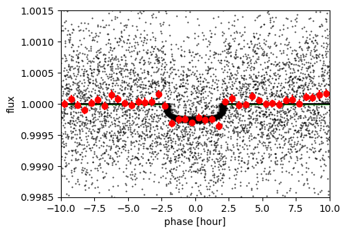
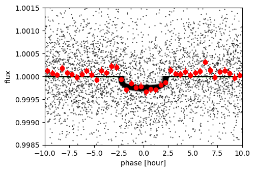
Figure 10: Stacked transits of Kepler-1705b (top) and Kepler-1705c (bottom). TTV-folded data are shown as black dots, bins of 30 mins are shown in red, and 1000 randomly selected posterior samples in black lines.

Table 3: Transit timings of Kepler-1705b and c in BJD-2454833.0.

median	$-\sigma$	$+\sigma$
Kepler-1705b
365.2143	-0.0109	0.0093
374.2501	-0.0103	0.0091
383.2838	-0.0099	0.0086
…
Kepler-1705c
374.3956	-0.0176	0.0201
385.6777	-0.0172	0.0194
396.9589	-0.0169	0.0185
…

The fit of the data was performed in two steps: a preliminary fit of the transit timings to the timing proxy shown in Fig. 8, followed by a photodynamic analysis of the light curve. Both steps use the TTVfast algorithm (Deck et al., 2014) for the computation of the transit timing for a set of initial conditions, and the samsam MCMC algorithm (see Delisle et al., 2018) to sample the posteriors. The light curve model was obtained by modelling the transit of each planet using the batman package (Kreidberg, 2015), shifting its centre to the dates of transits computed with TTVfast. The supersampling parameter was set to $29.42$ minutes to account for the long exposure of the dataset. Remaining long-term trends were modelled by a Gaussian process with a Matérn 3/2 kernel whose timescale was forced to be above one day to avoid interfering with the modelled transits. A jitter term was also added to all photometric measurements. The stellar parameters were retrieved from the Gaia-Kepler Stellar Properties Catalog (Berger et al., 2020) and given in Table 1. The effective temperature, ${\log g,}$ and metallicity were used to compute the quadratic limb-darkening coefficients $u_{1}$ and $u_{2}$ adapted to the Kepler spacecraft using LDCU. The fit was performed on the flattened DPCSAP flux, removing the data points at less than twice the transit duration of each transit of the 3.38-day candidate.

The resulting fitted and derived posteriors are given in Table 2. The fit converged toward a pair of similar-sized planets with masses of $4.61_{-0.45}^{+0.54}$ and $5.60_{-0.58}^{+0.66}$M_Earth, and radii of $2.04_{-0.14}^{+0.12}$ and $2.05_{-0.15}^{+0.14}$R_Earth, respectively. The eccentricities and longitude of periastron are strongly degenerate, as discussed in Sect. 5.2. The TTV-corrected stacked light curve of each planet can be seen in Fig. 10. The TTVs corresponding to 300 randomly chosen samples of the photodynamic fit are shown in Fig. 8 for comparison to the proxy generated from the confidence matrix.

The two planets are detected with S/Ns above 8.5. In addition, the anti-phased nature of the TTV signals shown in Fig. 8, the fact that these timings can be reproduced by a model of two planets in resonance, and the masses determined by the TTV analysis that are consistent with the derived radii, are independent confirmations of the planetary nature of the signals.

5 The resonant pair of Kepler-1705

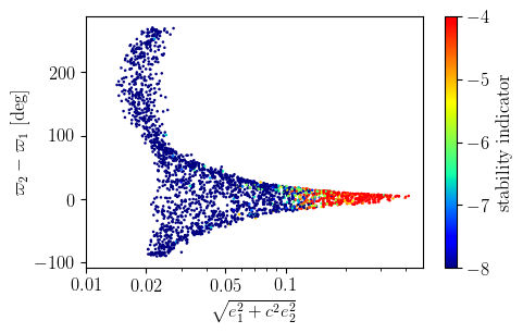
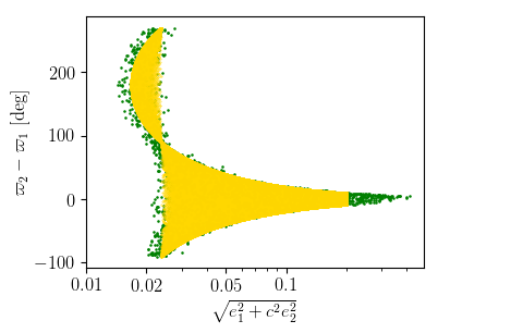
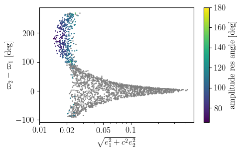
Figure 11: Top: Stability of the trajectories integrated from 2300 posterior samples, ranging from stable (blue) to unstable (red). Middle: Green dots show the projection of 2300 randomly selected samples of the posterior summarised in Table 2. Gold dots show the theoretical posterior discussed in section 5.2. Bottom: Smallest semi-amplitude between the two resonant angles (eq. 6). Grey dots indicate a circulation of both of them.

In this section, we study a subpopulation of 2300 randomly chosen samples from the posteriors presented in Table 2. Figure 11 shows the projection of these samples in the $(\sqrt{e_{1}^{2}+c^{2}e_{2}^{2}},\Delta\varpi=\varpi_{2}-\varpi_{1})$ plane ($c$ is defined in section 5.2). The $e_{j}$ and $\varpi_{j}$ represented here are the fitted initial conditions at the date 2455196.2294 BJD.

5.1 Stability

We verified the stability of the posteriors using the frequency analysis criterion (Laskar, 1990, 1993), using the same implementation as in Leleu et al. (2021). For this stability analysis, KOI4772.01 was added to the system using the ephemerides from the NASA exoplanet archive. Assuming an Earth-like density, we used a mass of $1.2e\!-\!05M_{\star}$. The top panel of Fig. 11 shows the resulting criterion for each initial condition, for integration over $10^{5}$ years. We find that the low-eccentricity part of the posterior is stable for more than $10^{6}$ years, which together correspond to more than 35 billion orbits of the resonant pair. However, a significant part of the high-eccentricity posterior is unstable on a short timescale (red dots in the top panel of Fig. 11). This instability is due to the presence of the inner planet; running the same analysis without KOI4772.01 gives a fully stable posterior.

5.2 Dynamics and TTV signal degeneracy

The middle panel of Figure 11 shows the 2300 randomly chosen samples from the posterior presented in Table 2. Plotted is a projection of these samples in the $(\sqrt{e_{1}^{2}+c^{2}e_{2}^{2}},\Delta\varpi=\varpi_{2}-\varpi_{1})$ plane (green dots), where ₁ and ₂ refer to the inner and outer planet of the pair, respectively, and $c$ is defined below, together with the distribution expected on theoretical grounds (gold dots). The latter can be understood as follows.

In addition to the usual energy and angular momentum integrals, coplanar systems near first-order commensurabilities have an additional approximate integral which is exact to first-order in the eccentricities when only the two resonant harmonics are included in the disturbing function (Sessin & Ferraz-Mello, 1984; Henrard & Lemaitre, 1986; Wisdom, 1986). Noting the resonant angles for the 5:4 resonance:

$$\phi_{1}=4\lambda_{1}-5\lambda_{2}+\varpi_{1}\ ;\ \phi_{2}=4\lambda_{1}-5\lambda_{2}+\varpi_{2}\,,$$ (6)

the integral is revealed by transforming the complex variables $z_{1}=e_{1}\,{\rm e}^{i\phi_{1}}$ and $z_{2}=e_{2}\,{\rm e}^{i\phi_{2}}$ to

$$u=z_{1}+cz_{2}\hskip 14.22636pt{\rm and}\hskip 14.22636ptv=cz_{1}-gz_{2},$$ (7)

where $c$ is a function of the Laplace coefficients and has a value of $c=-1.119$ for the 5:4 commensurability, and $g=(m_{2}/m_{1})\sqrt{a_{2}/a_{1}}$ (Mardling, in prep). We note that different scalings are used by different authors; for the purpose of this paper we use a scaling that reflects the values of the eccentricities. In terms of the transformed variables, the additional integral is simply $vv^{*}={\rm const}$, and its existence results in a one-dimensional curve in the $(\Re(u),\Im(u))$ plane, where $\Re(u)$ and $\Im(u)$ are the real and imaginary parts of $u$ (black curve in Figure 12).

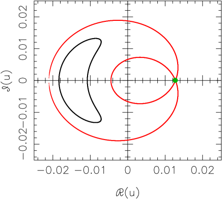
Figure 12: A phase-space plot showing the variation of the real and imaginary parts of the transformation variable $u$ (black curve: see eq. (7) for its definition in terms of the eccentricities and resonance angles). The best-fit solution has been used for the initial conditions of the black curve. As $u$ is constant over its theoretical distribution (yellow points in the second panel of Fig. 11), and varies little over its MCMC distribution (green points), the black curve represents in practice all points of the posterior. The phase space in which a system resides is resonant when there exists a solution containing a hyperbolic fixed point (green point in this figure) which has the same angular momentum as the system but a different energy. The separatrix (red curve) separates librating solutions from circulating solutions. The Kepler-1705 system is formally resonant because the phase space is resonant; it is in the librating state because it resides inside the separatrix. Being in the librating state allows determination of the planetary masses, independent of the eccentricities and the resonant state of the phase space (see text for discussion). We note that these curves are not surface-of-section projections but are true one-dimensional curves.

One can show that the TTV signal contains information about $u$ only, that is, it is blind to $v$ at first order in eccentricity (Mardling, in prep). As $u$ involves a linear combination of the quantities $e_{1}{\rm e}^{i\varpi_{1}}$ and $e_{2}{\rm e}^{i\varpi_{2}}$, solving the TTV-inverse problem results in degeneracies in the eccentricities and the reference-frame-independent angle $\phi_{2}-\phi_{1}=\varpi_{2}-\varpi_{1}$. Thus, while $u$ varies little over the posterior of a solution, $v$ is completely free, depending only on the imposed priors for the components of $e_{1}{\rm e}^{i\varpi_{1}}$ and $e_{2}{\rm e}^{i\varpi_{2}}$. The yellow dots in the middle panel of Figure 11 were generated by taking the best-fit solution, holding $u$ constant, and varying the real and imaginary parts of $v$ separately over the range $[-0.2,0.2]$. The resulting distribution closely matches the posterior for the solution.

We highlight the fact that the distribution is composed of two distinct components: points with $-90^{o}<\Delta\varpi<90^{o}$ and points with $90^{o}<\Delta\varpi<270^{o}$, corresponding to systems for which $\Delta\varpi$ librates around zero and $180^{o}$ respectively, but with circulation occurring near the boundary between the two.

As the stationary (fixed-point) values of $\phi_{1}$ and $\phi_{2}$ are zero and $180^{o}$ respectively, libration of both angles simultaneously can only occur around these values, and as a result $\Delta\varpi$ librates around $180^{o}$ in this circumstance. On the other hand, libration of $\Delta\varpi$ around zero can only occur when both angles circulate and have similar values.

Figure 12 shows that the Kepler-1705 system is in the librating resonant state, determined by the behaviour of the ‘resonant argument’, $\psi,$ defined such that $u=|u|{\rm e}^{i\psi}$. Librating systems (whether they are resonant or not) are characterised by two distinct non-commensurate resonant frequencies, one commonly referred to as the super-frequency (Lithwick et al., 2012), and a second which is usually significantly higher (Mardling, in prep; see also Nesvorny & Vokrouhlicky 2016). We note that these two frequencies are nearly degenerate for circulating systems. Therefore, if the observing baseline of a librating system is sufficiently long for both frequencies to be detected, there should be enough information in the signal to determine the planet masses independently of the eccentricities, that is, the mass–eccentricity degeneracy which plagues many TTV systems is broken (Mardling, in prep). We note that this does not depend on detecting the zeroth-order-in-eccentricity ‘chopping’ component of the TTV signal, which, although depending on the planet mass only, is generally much smaller than the resonant component (see, e.g. Linial et al 2018). For the Kepler-1705 system, the corresponding super-period is around 4000 d, while the second resonant period is around 1000 d; it is the latter which dominates the TTV signal as Figure 8 shows. Although the super-period is around four times the observing baseline, its effect on the signal allows for clear determination of the planet masses within 10%.

We briefly compare these results with the Hamiltonian formulation of the second fundamental model for resonance of Henrard & Lemaitre (1983). Using the one-degree-of-freedom model of first-order resonances presented in Deck et al. (2013), we computed the value of the Hamiltonian parameter $\Gamma^{\prime}$ (eq. 36 in the aforementioned paper), and found it to be relatively well constrained over the whole posterior, $\Gamma^{\prime}=2.43_{-0.35}^{+0.37}$, despite the degeneracies illustrated in Fig. 11. We computed the position of the separatrix for all the dots displayed in this figure. In all cases, the trajectories lie within the separatrix, ensuring that the system lies inside the 5:4 MMR (see Figure 12).

Finally, we note that a system can be in the librating resonant state even when both resonant angles circulate; this is the case when $\Delta\varpi$ librates around zero. Thus, the standard conclusion drawn that a system is not resonant unless at least one resonant angle librates is erroneous in this situation.

Classifying Kepler (near-)resonant pairs with respect to the period of the inner planet in the pair, Delisle & Laskar (2014) showed that systems where the period of the inner planet of the pair is smaller than 15 days tend to be near-resonant rather than inside the resonance, which can be explained by the tidal interaction with the star. The resonant state of the Kepler-1705 system can be explained by a lower dissipation in the planets, but could also be linked to the age of the system ($t_{\star}=2.59_{-1.61}^{+1.94}$ Gyr), if for example this latter is not yet sufficient to allow the tidal evolution to be fully effective.

5.3 Planetary spin dynamics

The spin of close-in, nearly circular planets is often assumed to be synchronised with the orbital motion due to strong tidal dissipation in the planets. In the case of Kepler-1705, the outer planet has a period of 11.28 d, and so one would indeed expect all the planetary spins to be in a synchronous state. However, planet–planet perturbations can drive the spin of rocky planets into asynchronous or chaotic states, even for nearly circular orbits (see Correia & Robutel, 2013; Leleu et al., 2016; Delisle et al., 2017; Correia & Delisle, 2019). In particular, as shown by Delisle et al. (2017), the TTVs are a very good probe with which to study the spin dynamics, because both TTVs and spin–orbit dynamics are dominated by the perturbations on the mean longitude of the planets. Planets with large TTVs, such as Kepler-1705b and c, thus also undergo strong perturbations in their spin dynamics, and could therefore be captured in non-synchronous states or could exhibit a chaotic evolution. At first approximation, the planet–planet perturbations introduce two new spin–orbit resonances surrounding the synchronous resonance (Correia & Robutel, 2013).

We studied the impact of these planet–planet perturbations on the spin evolution of Kepler-1705b and c. The details of this analysis are presented in Appendix D, and we briefly summarise our findings here. For Kepler-1705b, a permanent capture in the synchronous resonance is the most probable scenario, while a capture in the non-synchronous resonances does not seem possible. However, the spin of Kepler-1705b could undergo a chaotic evolution for a long time before tidal dissipation finally brings it to permanent capture in the synchronous resonance (see Delisle et al., 2017). For Kepler-1705c, a permanent capture in any of the three resonances (synchronous, super-synchronous, or sub-synchronous) is possible. As for Kepler-1705b, the spin of Kepler-1705c could also undergo a chaotic evolution for a long time before being permanently captured in one of these resonances.

6 Discussion and conclusion

6.1 Choices and caveats

In this paper we present a proof of concept: deep learning can be used to identify the track of a planet in a river diagram regardless of the presence of TTVs. To present this method, numerous choices were made, notably regarding the architecture of the neural network. Parts of the experimentation that was conducted prior to these choices are detailed in Appendix C.4. The cost function for the training of the model is also arbitrary, and is generally a trade-off between the recall (not missing the signature of a planet) and the false positive rate, both for the semantic segmentation (pixel of the river diagram belonging to a transit), and for the classification (track of the planet in the input matrix). Typically, cleaner periodograms can be obtained by reducing the false positive rate of the classification. On the other hand, a higher recall on the classification helps to recover planets with a lower S/N. The choice of training set can also influence the sensitivity of the model. In this paper we chose to train the model on a wide variety of systems in, or close to various MMRs, around any kind of star. Training per stellar type, or for a given orbital configuration, will probably provide better results for the dedicated task, provided that a large enough training set can be constructed.

Both the river diagram classifier and the pixel-level vetting of the RIVERS.deep matrix return confidence of the model on their task. These confidences are not likelihoods or probabilities. In that sense, this method can only be used to detect promising signals in large datasets, which in turn need to be analysed with a ‘classical’ study of the light curve, as performed in section 4.2.

6.2 Summary and Conclusion

For planets that are too small to induce individually detectable transits, TTVs could lead to erroneous estimations of the transit depth and duration, or even the absence of detection. For such planets, we present a method, using deep learning with tasks of semantic segmentation and image classification, to recover small planets with transit surveys with an approach that is robust to TTVs. This approach does not rely on the recognition of individual transits, nor on the stacking of the light curve to identify the candidate, but rather on the track that is drawn by the planet in a river diagram. We show that, in addition to the orbital period, individual transit timings can be estimated by the semantic segmentation task.

We illustrate the method by the detection and confirmation of a pair of super-Earths in a 5:4 MMR around Kepler-1705. Each of these planets has TTVs of $\sim 10$ h amplitude, and individual transit S/N of $\sim 1$. These planets do not appear when using the BLS algorithm. When comparing the resonant pair of Kepler-1705 to the previously known planets with large TTVs in Fig. 1, it appears that the RIVERS.deep method presented in this paper is indeed able to recover planets that had three times lower individual transit S/N than any other known planet with TTVs of more than 3 hours. The method therefore has the potential to alleviate the TTV bias in transit surveys. As this bias is due to orbital perturbations that happen on timescales longer than the orbital period, it is especially useful for observations with long baselines, such as Kepler, the polar observations of TESS, and the upcoming PLATO mission.

We find that Kepler-1705 is in a librating resonant state, and that this state varies little over the entire posterior of the photodynamic fit. Moreover, because the system is in this state the planet masses are well constrained, in contrast to systems in a circulating state for which the planet masses and eccentricities are degenerate. On the other hand, the eccentricities, resonant angles, and longitudes of periastron are not constrained, except for a lower limit for the eccentricities of around 0.01. This results from the fact that TTVs are sensitive to a component of the combined complex eccentricities only.

We also show that the significant orbital perturbations induced on Kepler-1705b and Kepler-1705c can significantly impact their spin dynamics. In both cases, a large chaotic area surrounds the synchronous spin–orbit resonance. The spin of the inner planet of the resonant pair should settle into the synchronous state after crossing the chaotic area. The outer planet can be locked either in the synchronous spin–orbit resonance, or in one of the sub- or super-synchronous resonances which originate from the orbital perturbation. This would have important consequences for the climate of the planet because a non-synchronous spin implies that the flux of the star is spread over the whole planetary surface. Regardless of which spin–orbit resonance these planets are trapped in, the orbital resonant motion induces forced oscillations of the spin with respect to the planet–star direction, which is a source of tidal dissipation.

The paucity of planets in MMR in the Kepler dataset is a subject that has been extensively studied in the last decade (e.g. Delisle et al., 2012; Fabrycky et al., 2014; Goldreich & Schlichting, 2014). Our study is a first step towards showing that part of this trend might be due to an observational bias. Recovering these small, (near-)resonant planets is valuable for our understanding of the formation and evolution of planetary systems, because the formation and evolution of resonant configurations are the markers of the dissipative evolution of planetary systems (see e.g. Henrard & Lemaitre, 1983; Lee & Peale, 2002; Terquem & Papaloizou, 2007; Papaloizou & Terquem, 2010; Delisle et al., 2012; Correia et al., 2018). In addition, for faint stars such as Kepler-1705, TTVs are currently our only means to estimate the mass of the planets, and hence their density and internal structures.

Appendix A TTV timescales

A two-body MMR is an orbital configuration in which the period of a pair of planets satisfies the following relation: $P_{2}/P_{1}\simeq(k+q)/k$, where $k$ and $q$ are integers, the latter being the order of the resonance. For a pair of planets inside a first-order ($q=1$) resonance, TTVs happen on a timescale:

$$P_{\text{TTV, $q=1$}}\propto f(m_{p}/m_{\star})^{-2/3}P_{orb}\,,$$ (8)

where $P_{orb}$ is comparable to the orbital period of the planets, $m_{p}$ is comparable to the mass of the planets, and $f$ is a factor or order 1 which increases as the libration amplitude increases (Nesvorný & Vokrouhlický 2016). In the co-orbital resonance ($q=0$), TTVs happen on the timescale (Vokrouhlický & Nesvorný 2014; Leleu et al. 2019):

$$P_{\text{TTV, $q=0$}}\propto f(m_{p}/m_{\star})^{-1/2}P_{orb}\,.$$ (9)

For a pair of planets near but not in a MMR of order $1$ or $2$, the TTVs happen on the period associated with the distance to the exact resonance $P_{2}/P_{1}=(k+q)/k$ in the frequency space:

$$P_{\text{TTV, near res}}=\frac{1}{(k+q)/P_{2}-k/P_{1}}\,.$$ (10)

In the neighbourhood of first-order MMRs, these TTVs are sinusoidal at first order in eccentricities (Lithwick et al. 2012; Agol & Deck 2016; Mardling 2018). A particular case of Eq. 10 for $q=0$ is referred to as the ‘chopping term’, which happens mainly for close pairs of planets near conjunction (Nesvorný & Vokrouhlický 2014).

Then, on longer timescales the evolution of eccentricities and inclinations —and associated angles— produce TTVs on secular timescales (see the Laplace-Lagrange theory Murray & Dermott 1999):

$$P_{\text{TTV, sec}}\propto(m_{p}/m_{\star})^{-1}P_{orb}\,.$$ (11)

Three-body resonances can also produce variation over this timescale. The effect of these configurations can add up linearly at first order.

Appendix B Effect of TTVs on transit depth

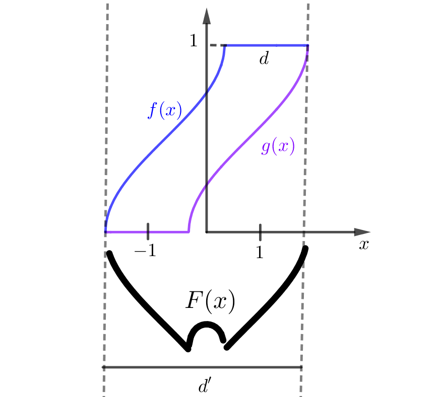
Figure 13: $f(x)$ gives the fraction of the time where $x$ is after the ingress, $g(x)$ gives the fraction of the time where $x$ is after the egress. $F(x)=g(x)-f(x)$ shows the shape of the stacked transit.

We estimate here the effect of TTVs on the estimated transit depth, when the TTVs are not modelled. We assume sinusoidal TTVs of period $2$ and of semi-amplitude $\sigma_{\text{TTV}}/2$. We note the duration of the underlying planetary transit $T_{\text{transit}}$. We normalise the phase of transit by the TTV semi-amplitude $\sigma_{\text{TTV}}/2$; and we parametrise the normalised phase by $x$, taking $x=0$ at the average mid-transit position (see Fig. 13). We assume the actual transits to be box-shaped, of depth $D,$ and of normalised duration $d=T_{\text{transit}}/(\sigma_{\text{TTV}}/2)$. Due to the symmetry of the $\sin$ function, we compute the average effect over half a TTV period. Noting $f(x)$ the fraction of the time when $x$ is after the ingress, and $g(x)$ the fraction of the time when $x$ is after the egress, we have (see Fig. 13):

$$f(x)= \arcsin(x+d/2)/\pi+1/2 \text{for}\ x\leq 1-d/2$$ (12)

$$f(x)= 1 \text{for}\ x\geq 1-d/2$$

and

$$g(x)= 0 \text{for}\ x\leq-1+d/2$$ (13)

$$g(x)= \arcsin(x-d/2)/\pi+1/2 \text{for}\ x\geq-1+d/2.$$

The flux loss due to the stacked transit at phase $x$ is given by $DF(x)$, where

$$\begin{aligned} F(x)=g(x)-f(x)\end{aligned},$$ (14)

which is the opposite of the fraction of time the phase $x$ is in transit, see Fig. 13. The recovered transit depth depends on the chosen stacked transit duration $d^{\prime}$:

$$\begin{aligned} \text{Smeared Depth}&=\frac{D}{d^{\prime}}\int^{d^{\prime}/2}_{-d^{\prime}/2}-F(x)dx\end{aligned}.$$ (15)

Choosing $d^{\prime}=2+d$, which results in a stacked transit that contains all the phases affected by the underlying transits as shown in Fig. 13, eq. 15 simplifies to:

Smeared Depth $$=dD/(2+d)\,.$$ (16)

We note that here we assume that the transits are stacked following the ‘true’ mean period of the planet. If the observation‘s cover only a fraction of the TTV period, a fit of the data can identify an instantaneous period that will lessen the smearing.

Appendix C Model description

C.1 Model architecture

C.1.1 Semantic segmentation model

The main building block of the semantic segmentation model is the convolution layer (Dumoulin & Visin 2016). A convolution layer is composed of multiple convolution filters which are matrices of floating point values (in our case of shape $3\times 3$). Applying a filter to an image (as depicted in Fig. 14) consists in sliding it over each pixel of the input and computing a weighted sum of the overlapped region. The weight associated to each pixel of the input is given by the corresponding value in the filter. During the training of the neural network, each filter will learn to highlight local patterns that will be useful for the next neural layers to work with. The goal of deep learning approaches is to let the model discover a deep hierarchy of features that enables it to solve the task at hand.

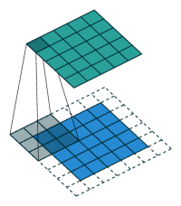
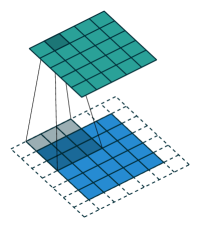
Figure 14: Application of a $3\times 3$ convolution filter (gray) on a $5\times 5$ input (blue) to generate a $5\times 5$ output (teal). To be able to center the filter on every pixel of the input (and therefore keep the same dimensions), we use one pixel of padding (dashed) with value 0 around the image.

The model used for the semantic segmentation task is a fully convolutional DenseNet (Jégou et al. 2017) illustrated in Fig. 15.

This architecture is particularly well suited to this job as there are multiple ‘paths’ from input to output in the model. Short paths are useful to analyse small local neighbourhoods and predict on a pixel-by-pixel basis which ones are more likely to belong to a transit. Long paths are more focused on deciding whether the global signal structure is coherent. By merging these two sources of features, the model is able to produce high-quality transit masks by looking for areas with lower average flux and a global structure that could be explained by a planet.

The first convolution layer of the model includes eight filters and the filter growth rate is of five (each convolution layer has five more filters than the previous one). The encoder and the decoder are both composed of five dense blocks. Dense blocks (Huang et al. 2017), illustrated in Fig. 16, are sequences of convolution layers with skip connections allowing the output to contain information from multiple levels of the feature hierarchy discovered by the network.

In the encoder, the dense blocks are interlaced with transition down blocks. The objective of these blocks is to reduce the resolution of the signal being processed in order to increase the scale of the pattern the next layers will process. This is performed using a maximum pooling operation (Scherer et al. 2010). This layer divides the width and the height of the signal by a factor of two by tiling its input using $2\times 2$ cells and replacing each cell by the maximum value it contains.

The bottleneck layer at the transition between the encoder and the decoder is used to refine the large-scale understanding the model has of the input, and is composed of a single dense block with eight convolution layers.

In the decoder, the dense blocks are interlaced with transition up blocks. The objective of these blocks is to increase the resolution of the signal being processed in order for the model to be able to produce an output of the same shape as its input (therefore producing a prediction for each of the pixels). This is performed using a variant of the convolution layer called a transposed convolution or fractionally strided convolution (Zeiler et al. 2010; Dumoulin & Visin 2016). As its name suggests, this operation increases the resolution of its input by applying a convolution operation in which the filter is moved by a fraction of a step. In our model, the filter is moved by half a step for each computation, therefore doubling the width and height of the signal.

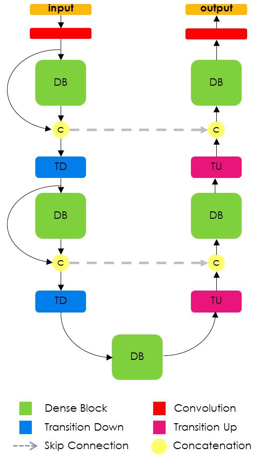
Figure 15: Architecture of the Tiramisu neural network used for the semantic segmentation task. The encoder (left part of the figure) is a subnetwork that works with an increasingly coarse representation of the data by using transition down blocks that reduce the resolution. The decoder (right part of the model) is a subnetwork that progressively combines low-resolution information coming from transition up blocks and high-resolution information coming from the encoder by skip connections. The bottleneck (dense block at the bottom of the figure) is used to refine the high level of understanding that the model has of the input.

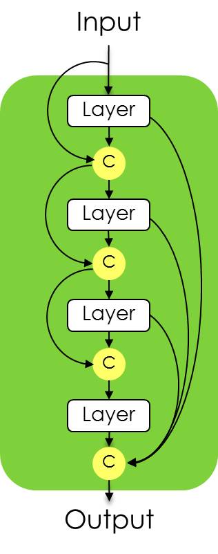
Figure 16: Architecture of one of the dense blocks that compose the Tiramisu model.

C.1.2 Classifier model

The classifier model takes the output of the semantic segmentation model as input and predicts whether or not the river diagram contains a perturbation.

The classifier is a convolutional neural network. Its base components are convolution blocks and linear blocks. A convolution block is composed of the following pieces:

• a convolution layer as defined in Section C.1.1,

• a 20% dropout layer (Srivastava et al. 2014) which randomly replaces 20% of the values of its input by 0 in order to improve generalisation and reduce dataset memorisation by the model (overfitting),

• a batch normalisation layer (Ioffe & Szegedy 2015) that accelerates the training procedure of the model by normalising its input,

• a ReLU activation function (Glorot et al. 2011) which is the simple non-linear function $f(x)=\text{max}(x,0)$. This function allows the model to approximate non-linear functions as it is otherwise entirely composed of linear combinations.

A linear block is composed of the following pieces:

• a linear (or fully connected) layer

• a 20% dropout layer,

• a batch normalisation layer,

• a ReLU activation, except for the very last block which uses a softmax activation. The softmax function normalises the raw output of the last layer into a probability distribution over all the classes of the classification task.

The sequence of convolution blocks is interlaced with maximum pooling operations (Scherer et al. 2010). This operation reduces the height and width of the array it is processing by a factor of two. It is used for two main reasons: (1) It allows us to mitigate the computation cost of increasing the number of filters in the following convolution blocks. We increase the number of filters in order to be able to recognise a greater variety of patterns. (2) It improves the translation invariance of the model. We would like the model decisions to be the same regardless of the positions of the planet track in the diagram. The maximum pooling operation is designed to loosen the spatial position of the patterns.

The sequence of blocks in the feature-extraction part of the model is given in Table 4.

Table 4: Sequence of blocks in the feature-extraction part of the model

layer	input channels	output channels
conv_block_1	2	32
conv_block_2	32	32
conv_block_3	32	32
max_pool_2d
conv_block_4	32	64
conv_block_5	64	64
conv_block_6	64	64
max_pool_2d
conv_block_7	64	128
conv_block_8	128	128
conv_block_9	128	128
max_pool_2d
conv_block_10	128	256
conv_block_11	256	256
conv_block_12	256	256
max_pool_2d

After flattening the output of these layers into a 1D vector, a sequence of three linear blocks with 256, 256, and 2 nodes is applied.

C.2 Training loss

When training neural network models, we have to define a differentiable loss function that quantifies how good the model prediction is compared to the desired value from the training dataset, the label or target. The loss function used to train our model is dependent on two sublosses, one for the semantic segmentation (pixel class prediction) and one for the classification (diagram class prediction).

The binary cross entropy loss ($BCE$) is defined as follows:

$$\text{BCE}(y,\hat{y},w)=w_{0}y\log(\hat{y})+w_{1}(1-y)\log(1-\hat{y}),$$ (17)

where $y$ is the target (either 0 or 1), $\hat{y}$ is the prediction of the model, and $w$ is the loss weight. This function will have a very low value when the confidence that the model has in the class $y$ is high and a high value otherwise. The goal of the training process is to minimise the value of this function on our training dataset.

We define the mask loss $\ell_{\text{m}}$ between a target mask $m\in\{0,1\}^{H\times W}$ and model output $\hat{m}\in[0,1]^{H\times W}$ as follows:

$$\ell_{\text{m}}(m,\hat{m},w)=\frac{1}{HW}\sum_{i=1}^{H}\sum_{j=1}^{W}BCE(m_{ij},\hat{m}_{ij},w).$$ (18)

The mask loss is effectively a classification loss at the pixel level of the diagram. In practice we give much more weight ($w_{1}$) to the perturbation class as this classification problem is very unbalanced. In the training dataset, diagrams containing perturbations only have around 2% of their pixel tagged as perturbation pixels.

We define the diagram loss $\ell_{d}$ between the diagram class $y$ and the model predicted class $\hat{y}$:

$$\ell_{\text{d}}(y,\hat{y},w)=BCE(y,\hat{y},w),$$ (19)

where $w$ is the loss weight.

The global loss of the model $\ell$ is a weighted sum of the mask loss and the diagram loss:

$$\ell(y,\hat{y},m,\hat{m},w,w_{\text{m}},w_{\text{d}})=w_{0}\ell_{\text{m}}(m,\hat{m},w_{\text{m}})+w_{1}\ell_{\text{d}}(y,\hat{y},w_{\text{d}}).$$ (20)

C.3 Training methodology

To train the model, we used the Adam optimizer (Kingma & Ba 2014) with a learning rate of $10^{-3}$ and a batch size of 45. The Adam algorithm is a variant of the classical stochastic gradient descent that uses the first and second moments of the gradients. The batch size is the number of samples that we used to approximate the gradient of the loss function during each optimisation step.

When training a neural network, data augmentation is typically used to help the model acquire invariants (such as rotation and noise invariance), virtually increase the diversity of the dataset, and reduce sample memorisation. It consists in randomly modifying the input of the model according to the augmentation strategy right before feeding them to the model. In our case, the data augmentation strategy consists in horizontal flips and random horizontal cyclical rotation of the diagrams.

In the training loop we used multiple algorithms to make the best use of our hardware.

We used a trick called gradient accumulation (Wolf 2018) to simulate our batch size of 45 as it did not fit in our GPU memory. This technique entails performing multiple forward and backward passes on different batches for each optimiser step.

We also used an algorithm called data echoing (Choi et al. 2019) to greatly speed up the training process. This technique involves performing multiple optimisation steps for each data loading by applying the different data augmentation. As fetching data from the disk is usually very slow, using this technique allows us to greatly reduce the impact of diagram loading on the training run-time. In our training runs, each diagram is used three times for each loading.

In order to improve the model ability to detect very low-magnitude signals among noise, we also implemented various curriculum learning strategies. Curriculum learning strategies consist in gradually increasing the difficulty of the target task along the training process. We experimented with multiple ways to modify the task:

• Progressively inserting samples of decreasing S/N to the training dataset. In our experiments, this approach does not improve the model performance when compared to starting the process with all of the sample at once.

• Adding a Gaussian noise with a mean of zero and slowly increasing the standard deviation to the model input. We call this algorithm the Gaussian virtual curriculum learning.

• Adding a more realistic noise of increasing amplitude to the model input. This noise is created from the input diagram by applying random cyclical rotations to each of its rows, scaling down the values to the desired amplitude and adding the result back to the original river diagram. The idea behind this methodology is to add a noise component to our sample that closely matches the one we could expect from this type of star. By rotating the rows by different amounts, we ensure that we are only left with noise. We call this algorithm the star virtual curriculum learning.

C.4 Experimentations

We trained models with and without using data augmentation. The overfitting phenomenon (in which the model metrics are much better on its training set than on its validation set) is greatly reduced by the data augmentation, and therefore we use it systematically.

The data-echoing algorithm increases the speed of the training process significantly. As mentioned in the main text, the variety of data used to approximate the gradients of the loss function is reduced, the quality of the approximation is therefore also reduced. By having a data augmentation strategy that greatly modifies a sample, this loss of quality does not significantly impact the training performance.

The virtual curriculum learning strategies have provided important metric improvements on previous model and dataset versions. We have yet to get such gains on our latest models. More hyperparameter tuning is needed to conclude whether this methodology can yield a boost in performance or not.

We have also tried multiple loss weighting strategies. Our experiments suggest that the bigger the weight on the semantic segmentation task the best the overall performances. Figures 17 and 18 illustrate the impact of various global loss weighting parameters. In these figures, the loss weighting is the following:

• For the ‘25% pxl 75% img’ model, the weight of the mask loss $w_{m}$ and the diagram loss $w_{d}$ are respectively 0.25 and 0.75.

• For the ‘ramping weight’ model, $w_{m}$ starts at a value of 0.01 and linearly increases to 0.75 from the epoch 10 to 30. At each step, the loss of the diagram loss is $w_{d}=1-w_{m}$.

• For all the ‘99% pxl 1% img’ models, $w_{m}=0.99$ and $w_{d}=0.01$.

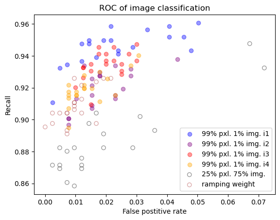
Figure 17: Receiver operating characteristic of the diagram classification task for different global loss weighting parameters. For each model, the metrics of the last 20 epochs are reported.

Figure 18: Receiver operating characteristic of the pixel classification task for different global loss weighting parameters. For each model, the metrics of the last 20 epochs are reported.

Appendix D Planetary spin dynamics

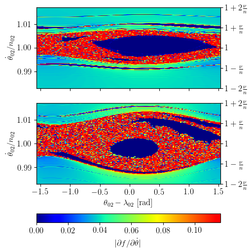
Figure 19: Spin evolution of Kepler-1705b for different values of the C22 coefficient. Top: Residual C22. Bottom: Synchronous averaged C22. Each pixel represents an initial condition for the spin of the planet. The x-axis shows the initial position of the ellipsoid with respect to the direction of the star, while the y-axis represent the initial spin rate. The colour of the pixels shows the derivative of the main frequency of the spin of the planet ($f$) with respect to the initial spin rate. This is an indicator of the spin state (Leleu et al. 2016): dark blue indicates a libration inside a spin-orbit resonance, cyan/green indicates a circulation of the spin, and red area indicates chaotic rotation.

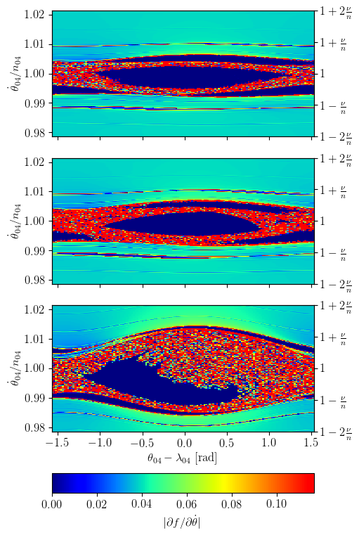
Figure 20: Spin evolution of Kepler-1705c for different values of the C22 coefficient, see Fig. 19 for explanations. Top: Residual C22. Middle: Asynchronous averaged C22. Bottom: Synchronous averaged C22.

In this Appendix, we study the impact of the planet–planet perturbations on the spin dynamics of Kepler-1705b and Kepler-1705c, following the method described in Delisle et al. (2017). Denoting the planet’s rotation angle with respect to an inertial line by $\theta$, the centre of the synchronous resonance is located at $\dot{\theta}\approx n$, while subsynchronous and super-synchronous resonances are located at $\dot{\theta}\approx n\pm\frac{\nu}{2}$, where $n$ is the planet mean-motion and $\nu$ is the perturbation’s angular frequency (Correia & Robutel 2013). The frequency $\nu$ is also the dominant frequency observed in the TTVs. The qualitative evolution of the spin depends on the width of the synchronous and sub or super-synchronous resonances, as well as the distance between them (Chirikov 1979). The width of the synchronous resonance, $\sigma$, depends on the planet’s asymmetry, and in particular on the $C_{22}$ Stokes gravity field coefficient. The width of the sub/super-synchronous resonances is of the order of $\sqrt{\alpha}\sigma$, where $\alpha$ is the TTVs angular amplitude (see Delisle et al. 2017).

We estimate the $C_{22}$ coefficients of Kepler-1705b and c following the method described in Delisle et al. (2017) (Appendices C and D). The planet asymmetry has two contributions, the permanent (or residual) deformation $C_{22,r}$ and the tidally induced deformation $C_{22,t}$. The permanent deformation can be roughly estimated from a scaling law obtained from observations of the Solar System planets (Yoder 1995)

$$C_{22,r}\sim 10^{-6}\left(\frac{R}{R_{\oplus}}\right)^{5}\left(\frac{M}{M_{\oplus}}\right)^{-5/2}.$$ (21)

As there are no analogues of Kepler-1705b or c in the Solar System, this scaling law only provides a very crude approximation of the permanent deformation of these planets, which we use in the absence of a more educated guess. We obtain $C_{22,r}\sim 8\times 10^{-7}$ for Kepler-1705b and $C_{22,r}\sim 5\times 10^{-7}$ for Kepler-1705c. The tidally induced deformation originates from the adjustment of the planet’s mass distribution to the external gravitational potential. The deformation of the planet depends on its internal structure and in particular its relaxation time. If the deformation were instantaneous, the planet’s shape would follow the variations of the external gravitational potential. On the contrary, if the relaxation time is much longer than the timescale of the gravitational potential variations, the deformation follows the average external gravitational potential. Outside of spin-orbit resonances, the tidal deformation averages out, but if the spin is captured in a resonance, the tidal deformation builds up. The average deformation depends on the considered spin-orbit resonance (Correia & Robutel 2013). Following Delisle et al. (2017), we compute the average $C_{22,t}$ for the synchronous and sub- or super-synchronous resonances, taking into account the amplitude of forced oscillations. The total $C_{22}$ is then the sum of the permanent and tidally induced contributions. For Kepler-1705b, we obtain $C_{22}\approx 3.5\times 10^{-6}$ in the synchronous resonance, while in the sub- and super-synchronous resonances, the contribution of the tidally induced deformation is negligible ($C_{22,t}\ll C_{22}\approx C_{22,r}=8\times 10^{-7}$). For Kepler-1705c, we obtain $C_{22}\approx 4.4\times 10^{-6}$ in the synchronous resonance and $C_{22}\approx 8\times 10^{-7}$ in the sub- and super-synchronous resonances.

We plot in Fig. 19 the phase portraits of the spin of Kepler-1705b using the estimated $C_{22,r}$ (top) and total $C_{22}$ in the synchronous resonance (bottom). These maps are obtained by n-body integration of the resonant pair and their star as point mass, in addition to the spin of one of the planets represented as an ellipsoid; see section 4.3 of Leleu et al. (2016) for more details. In the case of the permanent deformation alone, we observe a single large stable area corresponding to the synchronous resonance. This stable area is surrounded by a chaotic region which arises from the overlap of the synchronous resonance with the two sub- and super-synchronous resonances. When additionally accounting for the tidally induced deformation in the synchronous resonance, the chaotic area increases and the stable area shrinks but still exists. A permanent capture in the synchronous resonance is the most probable scenario for this planet, while a capture in the non-synchronous resonances does not seem possible. However, given the size of the chaotic area, the spin of Kepler-1705b could undergo a chaotic evolution for a long time before tidal dissipation finally brings it to permanent capture in the synchronous resonance (see Delisle et al. 2017).

The phase portraits of the spin of Kepler-1705c are shown in Fig. 20. For this planet, we plot three phase portraits, corresponding to the permanent deformation alone (top), the total deformation in the sub- or super-synchronous resonances (middle), and the total deformation in the synchronous resonance (bottom). Considering only the permanent deformation, we observe three stable areas corresponding to the three resonances (synchronous, sub-, and super-synchronous). The three resonances slightly overlap, which generates a chaotic area around the separatrices of these resonances. The three stable areas survive when taking into account the tidally induced deformation in the sub- and super-synchronous resonances. This suggests that a permanent capture in these non-synchronous resonances is possible for Kepler-1705c. Finally, when taking into account the tidally induced deformation in the synchronous resonance, the chaotic area extends and only the stable island corresponding to the synchronous resonance remains. Therefore, for this planet, permanent capture in any of the three resonances is possible. As for Kepler-1705b, the spin of Kepler-1705c could also undergo a chaotic evolution for a long time before being permanently captured in one of these resonances. The probability of capture in each resonance should be roughly proportional to its area in Fig. 20 (top). The sum of the areas of the two non-synchronous resonances is of the same order as the area of the synchronous resonance, which suggests that the spin of Kepler-1705c has a significant probability of being currently in a non-synchronous state. A more precise estimate of this probability would require a detailed study with long-term simulations including tidal dissipation, as was done in Delisle et al. (2017), which is beyond the scope of this article.