Short-Distance Structure of Unpolarized Gluon Pseudodistributions

Abstract

We present the results that form the basis for calculations of the unpolarized gluon parton distributions (PDFs) using the pseudo-PDF approach. We give the results for the most complicated box diagram both for gluon bilocal operators with arbitrary indices, and for combinations of indices corresponding to three matrix elements that are most convenient to extract the twist-2 invariant amplitude. We also present detailed results for the gluon-quark transition diagram. The additional results for the box diagram and the gluon-quark contribution may be used for extractions of the gluon PDF from different matrix elements, with a possible cross-check of the results obtained in this way.

I Introduction

Extraction of the parton distribution functions (PDFs) from lattice calculations attracts now a considerable interest (see Refs. Constantinou et al. (2021); Cichy and Constantinou (2019) for recent reviews and references to extensive literature). Modern efforts aim at getting PDFs $f(x)$ themselves rather than their $x^{N}$ moments. The recent progress in this endeavor has been stimulated by the paper Ji (2013) of X. Ji. Its basic proposal is to consider equal-time versions of nonlocal operators that define parton functions, such as PDFs, distribution amplitudes, generalized parton distributions, and transverse momentum dependent distributions. In the case of ordinary PDFs, the major object of Ji’s approach is a “parton quasi-distribution” (quasi-PDF) $Q(y,p_{3})$ Ji (2013, 2014). They produce PDFs obtained in the large-momentum $p_{3}\to\infty$ limit of quasi-PDFs.

Alternatively, one may use coordinate-space oriented methods, namely, the “good lattice cross sections” approach Ma and Qiu (2018a, b), the Ioffe-time analysis of equal-time correlators Braun and Müller (2008); Bali et al. (2018a, b) and the pseudo-PDF approach Radyushkin (2017a, b); Orginos et al. (2017). In these cases, parton distributions are extracted through taking the short-distance $z_{3}\to 0$ limit.

In converting the Euclidean lattice data into the light-cone PDFs one should take into account that both the $p_{3}\to\infty$ and $z_{3}\to 0$ limits are singular, and one needs to incorporate matching relations to perform the conversion.

The matching conditions in the quasi-PDF approach, were studied for quark Ji (2013); Xiong et al. (2014); Ji and Zhang (2015); Izubuchi et al. (2018) and gluon PDFs Wang and Zhao (2018); Wang et al. (2018, 2019), for the pion distribution amplitude (DA) Ji et al. (2015) and generalized parton distributions (GPDs) Ji et al. (2015); Xiong and Zhang (2015); Liu et al. (2019).

The matching relations in pseudo-PDF approach were also derived in several cases, in particular, for non-singlet PDFs Ji et al. (2017); Radyushkin (2018a, b); Zhang et al. (2018); Izubuchi et al. (2018). The procedure of lattice extraction of non-singlet GPDs and the pion DA within the pseudo-PDF framework was outlined in Ref. Radyushkin (2019), where the relevant matching conditions have been also derived.

In our earlier paper Balitsky et al. (2020) (see also Ref. Balitsky et al. (2021)) we have outlined the basic points of pseudo-PDF approach to extraction of unpolarized gluon PDFs, and have presented the one-loop matching conditions for a particular combination of gluon matrix elements, that has the “cleanest” projection on the twist-2 gluon PDF. These results have been used already in lattice extractions of the unpolarized gluon PDFs in Refs. Fan et al. (2021); Fan and Lin (2021) and Khan et al. (2021).

However, because of the letter nature of Ref. Balitsky et al. (2020), we have skipped there some intermediate expressions and also results for two other matrix elements that may be used for the gluon PDF extraction.

In the present paper, we present a full result for the most lengthy contribution of the “box” diagram, and also its projections onto all 3 matrix elements containing the “twist-2” invariant amplitude. We also give more details about our calculations of the gluon-quark mixing corrections both for these matrix elements and for matrix elements with arbitrary indices. The additional results given in the present paper may be used for extractions of the gluon PDF from two other matrix elements, which may give a possibility to cross-check the results obtained from different matrix elements.

The paper is organized as follows. In Section II, we study the structure of the matrix elements of the gluonic bilocal operators. In particular, we identify those that contain information about the twist-2 gluon PDF. In Section III, we discuss one-loop corrections, and specific properties of their ultraviolet and short-distance behavior. In subsection IIIf and Appendix A, we present our results for the most complicated “box” diagram. The subject of Section IV is the structure of perturbative evolution of the gluon operators, gluon-quark mixing and matching conditions. The result for the gluon-quark contribution generated by the gluon bilocal operator with arbitrary indices is given in Appendix B. Section V contains summary of the paper.

II Matrix elements

We are going to consider the nucleon spin-averaged matrix elements for operators composed of two-gluon-fields in the most general case when all four indices are not contracted

$${M}_{\mu\alpha;\nu\beta}(z,p)\equiv\langle p|\,G_{\mu\alpha}(z)\,[z,0]\,G_{\nu\beta}(0)|p\rangle\ ,$$ (2.1)

where $[z,0]$ stands for usual straight-line gauge link in the gluon (adjoint) representation

$$[x,y]~{}\equiv~{}{\rm Pexp}\Big{\{}ig\!\int_{0}^{1}\!dt~{}(x-y)^{\mu}\tilde{A}_{\mu}(tx+(1-t)y)\Big{\}}\ .$$ (2.2)

II.1 Invariant amplitudes

We want to decompose ${M}_{\mu\alpha;\nu\beta}(z,p)$ in several tensor structures accompanied by corresponding invariant amplitudes. The latter may be built from two available 4-vectors, namely $p_{\alpha}$, $z_{\alpha}$, and the metric tensor $g_{\alpha\beta}$. Building the tensors, we incorporate the antisymmetry of $G_{\rho\sigma}$ with respect to its indices. This gives Balitsky et al. (2020)

$${M}_{\mu\alpha;\nu\beta}(z,p)=$$

$$\left(g_{\mu\nu}p_{\alpha}p_{\beta}-g_{\mu\beta}p_{\alpha}p_{\nu}-g_{\alpha\nu}p_{\mu}p_{\beta}+g_{\alpha\beta}p_{\mu}p_{\nu}\right)\mathcal{M}_{pp}$$

$$+ \left(g_{\mu\nu}z_{\alpha}z_{\beta}-g_{\mu\beta}z_{\alpha}z_{\nu}-g_{\alpha\nu}z_{\mu}z_{\beta}+g_{\alpha\beta}z_{\mu}z_{\nu}\right)\mathcal{M}_{zz}$$

$$+ \left(g_{\mu\nu}z_{\alpha}p_{\beta}-g_{\mu\beta}z_{\alpha}p_{\nu}-g_{\alpha\nu}z_{\mu}p_{\beta}+g_{\alpha\beta}z_{\mu}p_{\nu}\right)\mathcal{M}_{zp}$$

$$+ \left(g_{\mu\nu}p_{\alpha}z_{\beta}-g_{\mu\beta}p_{\alpha}z_{\nu}-g_{\alpha\nu}p_{\mu}z_{\beta}+g_{\alpha\beta}p_{\mu}z_{\nu}\right)\mathcal{M}_{pz}$$

$$+ \left(p_{\mu}z_{\alpha}-p_{\alpha}z_{\mu}\right)\left(p_{\nu}z_{\beta}-p_{\beta}z_{\nu}\right)\mathcal{M}_{ppzz}$$

$$+ \left(g_{\mu\nu}g_{\alpha\beta}-g_{\mu\beta}g_{\alpha\nu}\right)\mathcal{M}_{gg}\ .$$ (2.3)

The amplitudes ${\cal M}$ are functions of the Lorentz invariants of the problem, i.e. the invariant interval $z^{2}$ and the Ioffe time Ioffe (1969) $(pz)\equiv-\nu$ (for further convenience we define $\nu$ with the minus sign).

Since the matrix element should be symmetric with respect to interchange of the fields, the functions $\mathcal{M}_{pp}$, $\mathcal{M}_{zz}$, $\mathcal{M}_{gg}$, $\mathcal{M}_{ppzz}$ and $\mathcal{M}_{pz}-\mathcal{M}_{zp}$ are even functions of $\nu$, while $\mathcal{M}_{pz}+\mathcal{M}_{zp}$ is odd in $\nu$.

II.2 “Twist-2” projection

The standard light-cone gluon distribution $f_{g}(x)$ is defined through the convolution $g^{\alpha\beta}{M}_{+\alpha;\beta+}(z,p)$, with the separation $z$ taken in the light-cone “minus” direction, $z=z_{-}$:

$$g^{\alpha\beta}{M}_{+\alpha;\beta+}(z_{-},p)=p_{+}^{2}\int_{-1}^{1}\differential x\,e^{ixp_{+}z_{-}}xf_{g}(x)\ .$$ (2.4)

Extracting the projection $g^{\alpha\beta}{M}_{+\alpha;\beta+}$ from the decomposition (2.3), we get

$$g^{\alpha\beta}{M}_{+\alpha;\beta+}(z_{-},p)=-2p_{+}^{2}\mathcal{M}_{pp}(\nu,0)\ .$$ (2.5)

This means that the gluon PDF is determined by the ${\cal M}_{pp}$ invariant amplitude

$$-\mathcal{M}_{pp}(\nu,0)=\frac{1}{2}\int_{-1}^{1}\differential x\,e^{-ix\nu}xf_{g}(x)\,\ .$$ (2.6)

In view of Eq. (2.6), our strategy is to choose matrix elements ${M}_{\mu\alpha;\lambda\beta}$ that contain ${\cal M}_{pp}$ in its parametrization, and ideally nothing else.

Having in mind lattice calculations, it is convenient to split the “+” components onto sum of space- and time-components. Also, due to antisymmetry of $G_{\rho\sigma}$ with respect to its indices, the combination $g^{\alpha\beta}{M}_{+\alpha;\beta+}(z,p)$ includes summation over the transverse indices $i,j=1,2$ only, and reduces to

$$g^{ij}{M}_{+i;j+}=-{M}_{+1;1+}-{M}_{+2;2+}$$

$$={M}_{0i;0i}+{M}_{3i;3i}+({M}_{0i;3i}+{M}_{3i;0i})\ .$$ (2.7)

with summation over $i=1,2$ implied.

II.3 Picking out $\mathcal{M}_{pp}$ amplitude

As found in Ref. Balitsky et al. (2020), there is an extension of the ${M}_{0i;i0}$ matrix element that contains the $\mathcal{M}_{pp}$ amplitude only,

$${M}_{0i;i0}+{M}_{ji;ij}= 2p_{0}^{2}\mathcal{M}_{pp}\ ,$$ (2.8)

where the summation both over $i$ and $j$ is implied.

One can apply a similar procedure on ${M}_{3i;i3}$. Using the expression

$${M}_{30;03} \equiv\bra{p}G_{30}(z)G_{03}(0)\ket{p}$$

$$=m^{2}\mathcal{M}_{pp}-z_{3}^{2}\mathcal{M}_{zz}-z_{3}p_{3}\left(\mathcal{M}_{zp}+\mathcal{M}_{pz}\right)$$

$$-p_{0}^{2}z_{3}^{2}\mathcal{M}_{ppzz}+\mathcal{M}_{gg}\ ,$$ (2.9)

we construct the combination:

$${M}_{3i;i3}+2{M}_{30;03}= 2p_{0}^{2}\mathcal{M}_{pp}-2p_{0}^{2}z_{3}^{2}\mathcal{M}_{ppzz}\ ,$$ (2.10)

which still has an additional term proportional to the $\mathcal{M}_{ppzz}$ invariant amplitude. Another minimally contaminated combination is given by

$${M}_{0i;i3}+ {M}_{3i;i0}=4p_{0}p_{3}\mathcal{M}_{pp}+2p_{0}z_{3}\left(\mathcal{M}_{pz}+\mathcal{M}_{zp}\right)\ .$$ (2.11)

II.4 Multiplicatively renormalizable combinations

Off the light cone, the ${M}_{\mu\alpha;\lambda\beta}$ matrix elements have extra ultraviolet divergences related to presence of the gauge link. For any set of its indices $\{\mu\alpha;\lambda\beta\}$, each matrix element is multiplicatively renormalizable with respect to these divergences Li et al. (2019), but in general, with different anomalous dimensions.

In Ref. Zhang et al. (2019), it was established that the combinations represented in Eq. (2.7), namely, ${M}_{0i;i0}$, ${M}_{3i;i3}$, ${M}_{0i;i3}+{M}_{3i;i0}$ (and also ${M}_{0i;i3}-{M}_{3i;i0}$), with summation over transverse indices $i$, are each multiplicatively renormalizable at the one-loop level. Furthermore, as noted in Ref. Balitsky et al. (2020), the combination $G_{ij}G_{ij}$ (with summation over transverse $i,j$) has the same one-loop UV anomalous dimension as ${M}_{0i;i0}$, while the matrix element $G_{30}G_{03}$ has the same one-loop UV anomalous dimension as ${M}_{3i;i3}$. Hence, the combinations of Eqs. (2.8) and (2.10) are multiplicatively renormalizable at the one-loop level.

II.5 Reduced Ioffe-time distribution

Within the pseudo-PDF approach Radyushkin (2017a), the link-related UV divergences are eliminated through introducing the reduced Ioffe-time distribution. Namely, for each multiplicatively renormalizable amplitude $\mathcal{M}$ we build the ratio

$${\mathfrak{M}}(\nu,z_{3}^{2})\equiv\frac{{\mathcal{M}}(\nu,z_{3}^{2})}{{\mathcal{M}}(0,z_{3}^{2})}\ ,$$ (2.12)

in which the link-related UV divergent $Z(z_{3}^{2}\mu^{2}_{UV})$ factors generated by the vertex and link self-energy diagrams cancel. As a result, the small-$z_{3}^{2}$ dependence of the reduced pseudo-ITD ${\mathfrak{M}}(\nu,z_{3}^{2})$ comes from the logarithmic DGLAP evolution effects only.

III One loop corrections

Below, we briefly summarize the results on “non-box” one-loop corrections presented in Ref. Balitsky et al. (2020), and then discuss a rather lengthy contribution of the box diagram that was presented there in part only.

III.1 Link self-energy contribution

The self-energy correction for the gauge link is given by the simplest diagram (see Fig. 1). In lattice perturbation theory, it was calculated at one loop in Ref. Chen et al. (2017). An important property of this contribution is the presence of a $\sim z_{3}/a_{L}$ linear term, where $a_{L}$ is the lattice spacing that provides here the ultraviolet cut-off.

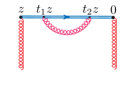
Figure 1: Self-energy-type correction for the gauge link.

Such corrections clearly factorize into a $\nu$-independent factor, and cancel in the ratio (2.12), so that their explicit form is not essential in the pseudo-PDF approach. Still, in dimensional regularization, one has

$$-{g^{2}N_{c}\over 4\pi^{2}[(-z^{2}\mu_{\rm UV}^{2}+i\epsilon)]^{{d\over 2}-2}}{\Gamma\big{(}{d/2}-1\big{)}\over(3-d)(4-d)}$$

$$\times G_{\mu\alpha}(z)G_{\lambda\beta}(0)\ ,$$ (3.1)

where the pole for $d=3$ ($d=4$) corresponds to the linear (logarithmic) UV divergences present in this diagram.

III.2 Vertex contribution

There are also vertex diagrams involving gluons that connect the gauge link with the gluon lines, see Fig. 2.

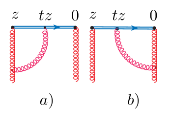
Figure 2: Vertex diagrams with gluons coming out of the gauge link.

We use the method of calculation described in Ref. Balitsky and Braun (1989). It is based on the background-field technique, with the gluon propagator taken in the “background-Feynman” (bF) gauge Balitsky and Braun (1989). The full, “uncontracted” vertex contribution is given by

$$\mathcal{O}_{\mu\alpha;\nu\beta}^{\rm vertex}=\,\frac{g^{2}N_{c}\Gamma(d/2-1)}{4\pi^{2}(-z^{2})^{d/2-1}}$$

$$\times\int_{0}^{1}\differential u\left\{\left(\frac{u^{3-d}-u}{d-2}\right)G_{\mu\alpha}(\bar{u}z)\left(z_{\beta}G_{z\nu}(0)-z_{\nu}G_{z\beta}(0)\right)\right.$$

$$\quad\left.+\left(\frac{u^{3-d}-u}{d-2}\right)\left(z_{\alpha}G_{z\mu}(\bar{u}z)-z_{\mu}G_{z\alpha}(\bar{u}z)\right)G_{\nu\beta}(0)\right\}$$

$$\quad+\frac{g^{2}N_{c}\Gamma(d/2-2)}{8\pi^{2}(-z^{2})^{d/2-2}}$$

$$\quad\times\int_{0}^{1}\differential u\,2\left[\frac{u^{3-d}-1}{d-3}\right]_{+}G_{\mu\alpha}(\bar{u}z)G_{\nu\beta}(0)\ .$$ (3.2)

In this expression, just one of the fields in the $G_{\mu\alpha}(z)G_{\lambda\beta}(0)$ operator is corrected, while another remains intact. In particular, the diagram 2a changes $G_{\mu\alpha}(z)$ into the sum of two terms. One of them contains UV divergences, while the other one is UV finite. The UV-divergent term is given by

$$\frac{N_{c}g^{2}}{4\pi^{2}}\frac{\Gamma(d/2-1)}{(d-2)(-z^{2})^{d/2-1}}\int_{0}^{1}\differential u\,\left(u^{3-d}-u\right)$$

$$\quad\times\left(z_{\alpha}G_{z\mu}(\bar{u}z)-z_{\mu}G_{z\alpha}(\bar{u}z)\right)\ ,$$ (3.3)

where $G_{z\sigma}\equiv z^{\rho}G_{\rho\sigma}$ and $\bar{u}\equiv 1-u$. The overall $d$-dependent factor here is finite for $d=4$, but the $u$-integral diverges at the lower limit. The divergence disappears if one uses the UV regularization by taking $d=4-2\varepsilon_{\rm UV}$, which converts it into a pole at $\varepsilon_{\rm UV}=0$.

Since the UV divergence comes from the $u\to 0$ integration, we can isolate it by taking $\bar{u}=1$ in the gluonic field, which gives

$$\frac{N_{c}g^{2}}{8\pi^{2}}\frac{\Gamma(d/2-1)}{(-z^{2})^{d/2-1}}\frac{1}{4-d}\left(z_{\alpha}G_{z\mu}(z)-z_{\mu}G_{z\alpha}(z)\right)\ .$$ (3.4)

The remainder is given by

$$\frac{N_{c}g^{2}}{4\pi^{2}}\frac{\Gamma(d/2-1)}{(d-2)(-z^{2})^{d/2-1}}\int_{0}^{1}\differential u\,\left[u^{3-d}-u\right]_{+(0)}$$

$$\quad\times\left(z_{\alpha}G_{z\mu}(\bar{u}z)-z_{\mu}G_{z\alpha}(\bar{u}z)\right)\ ,$$ (3.5)

where the plus-prescription at $u=0$ is defined as

$$\int_{0}^{1}\differential u\left[f(u)\right]_{+(0)}g(u)=\int_{0}^{1}\differential uf(u)[g(u)-g(0)]\ .$$ (3.6)

The second, UV finite term from the diagram 2a is given by

$$\quad\frac{N_{c}g^{2}}{8\pi^{2}}\frac{\Gamma(d/2-2)}{({d-3})(-z^{2})^{d/2-2}} \int_{0}^{1}\differential u\left[u^{3-d}-1\right]_{+(0)}$$

$$\quad\times G_{\mu\alpha}(\bar{u}z)G_{\lambda\beta}(0)\ .$$ (3.7)

Note that the gluonic operator in Eq. (3.7) has the same tensor structure as the original operator $G_{\mu\alpha}(z)G_{\beta\nu}(0)$ differing from it just by rescaling $z\to\bar{u}z$. There is no mixing with operators of a different type. The $u$-integral in this case does not diverge for $d=4$, but the overall $\Gamma(d/2-2)$ factor has a pole $1/(d-4)$.

Formally, there is also a pole $1/(d-3)$, corresponding to a linear UV divergence. However, the singularity for $d=3$ is eliminated by the $\left[u^{3-d}-1\right]$ combination in the integrand. One may say that the linear divergences present in “$u^{3-d}$” and “$-1$” parts cancel each other.

The remaining $1/(d-4)$ pole corresponds to a collinear divergence developed because all the propagators correspond to massless particles.

III.3 Gluon self-energy diagrams

Another simple type of one-loop corrections is represented by the gluon self-energy diagrams, one of which is shown in Fig. 3a. These diagrams have both the UV and collinear divergences. The combined contribution of the Fig. 3 diagrams and their left-leg analogs is given by

$${g^{2}N_{c}\over 8\pi^{2}}\frac{1}{2-d/2}\left[2-\frac{\beta_{0}}{2N_{c}}\right]G_{\mu\alpha}(z)G_{\lambda\beta}(0)\ ,$$ (3.8)

where $\beta_{0}=11N_{c}/3$ in gluodynamics, so that the terms in the square bracket combine into 1/6.

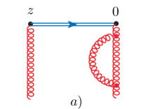
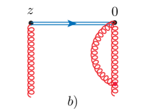
Figure 3: Gluon self-energy-type insertions into the right leg.

III.4 Box diagram

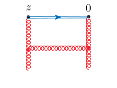
Figure 4: Box diagram.

The most complicated technically is the calculation of the “box” diagram which contains a gluon exchange between two gluon lines (see Fig. 4). This diagram does not have UV divergences, but it has DGLAP $\log z_{3}^{2}$ contributions. In contrast to the vertex diagrams, the original $G_{\mu\alpha}(z)G_{\nu\beta}(0)$ operator generates now a mixture of bilocal operators corresponding to various projections of $G_{\mu\alpha}(uz)G_{\nu\beta}(0)$ onto the structures built from vectors $p$, $z$ and the metric tensor $g$.

Our result for arbitrary indices $\mu\alpha\nu\beta$ is given in the Appendix A. It is presented in the operator form, however, it contains only those operators that survive in the forward case, i.e., the operators that have the form of a full derivative are abandoned. Still, the expression is rather lengthy. Furthermore, we mostly need it for particular combinations of indices corresponding to matrix elements ${M}_{0i;i0}+{M}_{ji;ij}$, ${M}_{3i;i3}+2{M}_{30;03}$ and ${M}_{0i;i3}+{M}_{3i;i0}$ that contain the $M_{pp}$ invariant amplitude and are listed in Eqs. (2.8), (2.10) and (2.11). To shorten the formulas, let us introduce the following notations for the bilocal operators corresponding to these matrix elements.

$${\mathcal{O}}_{00}(z_{1},z_{2})= G_{0i}(z_{1})G_{i0}(z_{2})+G_{ij}(z_{1})G_{ji}(z_{2})\ ,$$ (3.9)

$${\mathcal{O}}_{33}(z_{1},z_{2})= G_{3i}(z_{1})G_{i3}(z_{2})+2G_{30}(z_{1})G_{03}(z_{2})\ ,$$ (3.10)

$${\mathcal{O}}_{03}^{+}(z_{1},z_{2})= G_{0i}(z_{1})G_{i3}(z_{2})+G_{3i}(z_{1})G_{i0}(z_{2})\ .$$ (3.11)

In the case of ${\mathcal{O}}_{00}(z,0)$ and ${\mathcal{O}}_{33}(z,0)$ operators, the box diagram produces the following corrections

$${\mathcal{O}}_{00}(z,0)\stackrel{{\scriptstyle\rm box}}{{\longrightarrow}} \,-\frac{g^{2}N_{c}\Gamma(d/2-1)}{4\pi^{2}\left(-z^{2}\right)^{d/2-2}}\int_{0}^{1}\differential u\,\left(u\bar{u}+\frac{\bar{u}^{3}}{3}\right){\mathcal{O}}_{33}(uz,0)$$

$$\quad+\frac{N_{c}\Gamma(d/2-2)}{8\pi^{2}\left(-z^{2}\right)^{d/2-2}}\int_{0}^{1}\differential u\left\{\vphantom{\frac{1}{2}}\right.\left(\bar{u}\left(u^{2}+1\right)-2u\right){\mathcal{O}}_{00}(uz,0)+\bar{u}\left(u^{2}+1\right){\mathcal{O}}_{33}(uz,0)\left.\vphantom{\frac{1}{2}}\right\}\ ,$$ (3.12)

$${\mathcal{O}}_{33}(z,0)\stackrel{{\scriptstyle\rm box}}{{\longrightarrow}} \,-\frac{g^{2}N_{c}\Gamma(d/2-1)}{4\pi^{2}\left(-z^{2}\right)^{d/2-2}}\int_{0}^{1}\differential u\left\{\vphantom{\frac{1}{2}}\left(\bar{u}+u\bar{u}+\frac{\bar{u}^{3}}{3}\right){\mathcal{O}}_{33}(uz,0)-\bar{u}{\mathcal{O}}_{00}(uz,0)\right\}$$

$$\quad+\frac{N_{c}\Gamma(d/2-2)}{8\pi^{2}\left(-z^{2}\right)^{d/2-2}}\int_{0}^{1}\differential u\left\{\vphantom{\frac{1}{2}}\right.\left(\bar{u}\left(u^{2}+1\right)-2u\right){\mathcal{O}}_{33}(uz,0)+\bar{u}\left(u^{2}+1\right){\mathcal{O}}_{00}(uz,0)\left.\vphantom{\frac{1}{2}}\right\}\ .$$ (3.13)

One can see that the box diagram contribution for each of them involves matrix elements of both the operators ${\mathcal{O}}_{00}(uz,0)$ and ${\mathcal{O}}_{33}(uz,0)$. Thus, these two operators mix here with each other. Furthermore, matrix elements of both of them contain the $\mathcal{M}_{pp}$ invariant amplitude. Thus, it is interesting to rewrite Eqs. (III.4) , (III.4) in terms of the invariant functions:

$$\mathcal{M}_{pp}(\nu,z^{2}) \stackrel{{\scriptstyle\rm box}}{{\longrightarrow}}\,-\frac{g^{2}N_{c}\Gamma(d/2-1)}{4\pi^{2}\left(-z^{2}\right)^{d/2-2}}\int_{0}^{1}\differential u\,\left(u\bar{u}+\frac{\bar{u}^{3}}{3}\right)\left[\mathcal{M}_{pp}(u\nu,z^{2})-z_{3}^{2}\mathcal{M}_{ppzz}(u\nu,z^{2})\right]$$

$$\quad+\frac{g^{2}N_{c}\Gamma(d/2-2)}{8\pi^{2}\left(-z^{2}\right)^{d/2-2}}\int_{0}^{1}\differential u\left\{\vphantom{\frac{1}{2}}\right.2\left(\bar{u}\left(u^{2}+1\right)-u\right)\,\mathcal{M}_{pp}(u\nu,z^{2})-\bar{u}\left(u^{2}+1\right)z_{3}^{2}\mathcal{M}_{ppzz}(u\nu,z^{2})\left.\vphantom{\frac{1}{2}}\right\}\ ,$$ (3.14)

$$\mathcal{M}_{pp}(\nu,z^{2})-z_{3}^{2}\mathcal{M}_{ppzz}(\nu,z^{2})\stackrel{{\scriptstyle\rm box}}{{\longrightarrow}} \,-\frac{g^{2}N_{c}\Gamma(d/2-1)}{4\pi^{2}\left(-z^{2}\right)^{d/2-2}}\int_{0}^{1}\differential u\left\{\vphantom{\frac{1}{2}}\left(u\bar{u}+\frac{\bar{u}^{3}}{3}\right)\mathcal{M}_{pp}(u\nu,z^{2})\right.$$

$$\quad\quad\quad\quad\quad\quad\quad\quad\quad\quad\quad\quad\left.-\left(u\bar{u}+\frac{\bar{u}^{3}}{3}+\bar{u}\right)z_{3}^{2}\mathcal{M}_{ppzz}(u\nu,z^{2})\right\}$$

$$\quad+\frac{g^{2}N_{c}\Gamma(d/2-2)}{8\pi^{2}\left(-z^{2}\right)^{d/2-2}}\int_{0}^{1}\differential u\left\{\vphantom{\frac{1}{2}}\right.2\left(\bar{u}\left(u^{2}+1\right)-u\right)\mathcal{M}_{pp}(u\nu,z^{2})$$

$$\quad\quad\quad\quad\quad\quad\quad\quad\quad\quad\quad\quad\quad-[\bar{u}\left(u^{2}+1\right)-2u]\,z_{3}^{2}\mathcal{M}_{ppzz}(u\nu,z^{2})\left.\vphantom{\frac{1}{2}}\right\}\ .$$ (3.15)

These relations have a very similar structure and, in fact, coincide if one discards the $\mathcal{M}_{ppzz}$ terms. Taking the difference of these expressions gives a very simple result for the box correction to $\mathcal{M}_{ppzz}$

$$\mathcal{M}_{ppzz}(\nu,z^{2})\stackrel{{\scriptstyle\rm box}}{{\longrightarrow}} \,-\frac{g^{2}N_{c}\Gamma(d/2-1)}{4\pi^{2}\left(-z^{2}\right)^{d/2-2}}\int_{0}^{1}\differential u\,\bar{u}\,\mathcal{M}_{ppzz}(u\nu,z^{2})-\frac{g^{2}N_{c}\Gamma(d/2-2)}{4\pi^{2}\left(-z^{2}\right)^{d/2-2}}\int_{0}^{1}\differential u\,u\,\mathcal{M}_{ppzz}(u\nu,z^{2})\ .$$ (3.16)

The situation is simpler for the ${\mathcal{O}}_{03}^{+}(z,0)$ operator, for which the box diagram contribution is expressed through the ${\mathcal{O}}_{03}^{+}(uz,0)$ operator only,

$${\mathcal{O}}_{03}^{+}(z,0)\stackrel{{\scriptstyle\rm box}}{{\longrightarrow}} \,\frac{g^{2}N_{c}\Gamma(d/2-1)}{4\pi^{2}\left(-z^{2}\right)^{d/2-2}}\int_{0}^{1}\differential u\,\left(u\bar{u}+\frac{2}{3}{\bar{u}^{3}}\right){\mathcal{O}}_{03}^{+}(uz,0)$$

$$+\frac{N_{c}\Gamma(d/2-2)}{4\pi^{2}\left(-z^{2}\right)^{d/2-2}}\int_{0}^{1}\differential u\,\left(\bar{u}\left(u^{2}+1\right)-u\right){\mathcal{O}}_{03}^{+}(uz,0)\ .$$ (3.17)

In all the cases, Eqs. (III.4), (III.4), and (III.4), the $\Gamma(d/2-2)$ terms are singular for $d=4$, which results in $\log(-z^{2})$ terms generating the DGLAP evolution. The $\Gamma(d/2-1)$ terms are singular for $d=2$, which corresponds to the fact that the gluon propagator in two dimensions has a logarithmic $\log(-z^{2})$ behavior in the coordinate space. For $d=4$, these terms are finite. Note that, unlike the vertex part, the box contribution does not have the plus-prescription form.

IV DGLAP evolution structure

Adding the results for all the diagrams discussed above, we get the following expressions for their combined contribution for the 3 operator combinations listed in Eq. (3.11)

$${M}_{0i;i3}+{M}_{3i;i0}=4p_{0}p_{3}\mathcal{M}_{pp}\left(\nu,z_{3}^{2}\right)+2p_{0}z_{3}\left(\mathcal{M}_{pz}\left(\nu,z_{3}^{2}\right)+\mathcal{M}_{zp}\left(\nu,z_{3}^{2}\right)\right)$$

$$\to\frac{g^{2}N_{c}}{8\pi^{2}}\int_{0}^{1}\differential u\left\{\left[\left(\frac{3}{2}-\frac{1}{6}\right)\log(z_{3}^{2}\mu_{\rm UV}^{2}\frac{e^{2\gamma_{E}}}{4})+2\right]\delta(\bar{u})+\left[u-3\frac{u}{\bar{u}}-4\frac{\log(\bar{u})}{\bar{u}}\right]_{+}+2\left(\bar{u}u+\frac{2}{3}\bar{u}^{3}\right)\right.$$

$$\quad\left.-2\log(z_{3}^{2}\mu_{\rm IR}^{2}\frac{e^{2\gamma_{E}}}{4})\left[\frac{(1-u\bar{u})^{2}}{\bar{u}}\right]_{+}\right\}\,\left(4p_{0}p_{3}\mathcal{M}_{pp}\left(u\nu,z_{3}^{2}\right)+2up_{0}z_{3}\left(\mathcal{M}_{pz}\left(u\nu,z_{3}^{2}\right)+\mathcal{M}_{zp}\left(u\nu,z_{3}^{2}\right)\right)\right)\ ,$$ (4.1)

$$\frac{M_{0i;i0}+M_{ij;ji}}{2p_{0}^{2}}=\mathcal{M}_{pp}\left(\nu,z_{3}^{2}\right)$$

$$\to\frac{g^{2}N_{c}}{8\pi^{2}}\int_{0}^{1}\differential u\left\{\left(\left(1-{1\over 6}\right)\log\left(z_{3}^{2}\mu^{2}_{\rm UV}\frac{e^{2\gamma_{E}}}{4}\right)+2\right)\delta\left(\bar{u}\right)-\left({1\over 2}\delta\left(\bar{u}\right)+\left[{2\over 3}\left(1-u^{3}\right)+{4u+4\log(\bar{u})\over\bar{u}}\right]_{+}\right)\right.$$

$$\quad\left.-\log\left(z_{3}^{2}\mu^{2}_{\rm IR}\frac{e^{2\gamma_{E}}}{4}\right)\left[{2\left(1-u\bar{u}\right)^{2}\over\bar{u}}\right]_{+}\right\}\,\mathcal{M}_{pp}\left(u\nu,z_{3}^{2}\right)$$

$$\quad+\frac{g^{2}N_{c}}{8\pi^{2}}\int_{0}^{1}\differential u\left\{{2\over 3}\left(1-u^{3}\right)+\log\left(z_{3}^{2}\mu^{2}_{\rm IR}\frac{e^{2\gamma_{E}}}{4}\right)\bar{u}\left(u^{2}+1\right)\right\}\,u^{2}z_{3}^{2}\mathcal{M}_{ppzz}\left(u\nu,z_{3}^{2}\right)\ ,$$ (4.2)

$$\frac{M_{3i;i3}+2M_{30;03}}{2p_{0}^{2}}=\mathcal{M}_{pp}\left(\nu,z_{3}^{2}\right)-z_{3}^{2}\mathcal{M}_{ppzz}\left(\nu,z_{3}^{2}\right)$$

$$\to\frac{g^{2}N_{c}}{8\pi^{2}}\int_{0}^{1}\differential u\left\{\left(\left(2-{1\over 6}\right)\log\left(z_{3}^{2}\mu^{2}_{\rm UV}\frac{e^{2\gamma_{E}}}{4}\right)+2\right)\delta\left(\bar{u}\right)-\left({1\over 2}\delta\left(\bar{u}\right)+\left[{2\over 3}\left(1-u^{3}\right)+{2u^{2}+4\log(\bar{u})\over\bar{u}}\right]_{+}\right)\right.$$

$$\quad\left.-\log\left(z_{3}^{2}\mu^{2}_{\rm IR}\frac{e^{2\gamma_{E}}}{4}\right)\left[{2\left(1-u\bar{u}\right)^{2}\over\bar{u}}\right]_{+}\right\}\left(\mathcal{M}_{pp}\left(u\nu,z_{3}^{2}\right)-u^{2}z_{3}^{2}\mathcal{M}_{ppzz}\left(u\nu,z_{3}^{2}\right)\right)$$

$$\quad-\frac{g^{2}N_{c}}{8\pi^{2}}\int_{0}^{1}\differential u\left\{2\bar{u}+\log(z_{3}^{2}\mu_{\rm IR}^{2}\frac{e^{2\gamma_{E}}}{4})\bar{u}\left(u^{2}+1\right)\right\}u^{2}z_{3}^{2}\mathcal{M}_{ppzz}\left(u\nu,z_{3}^{2}\right)\ .$$ (4.3)

All these combinations contain the $\log\left(z_{3}^{2}\mu^{2}_{\rm IR}\frac{e^{2\gamma_{E}}}{4}\right)$ evolution term accompanied by the $gg$-component of the Altarelli-Parisi (AP) kernel

$$B_{gg}(u)=2\left[\frac{(1-u\bar{u})^{2}}{\bar{u}}\right]_{+}\ .$$ (4.4)

However, they have different $z_{3}$-independent parts, as a result of mixing with “higher-twist” functions $\mathcal{M}_{zp}+\mathcal{M}_{pz}$ in Eq. (IV), and $\mathcal{M}_{ppzz}$ in Eqs. (IV) and (IV). The kernel (4.4) has the plus-prescription structure reflecting the fact that, in the local limit, ${\mathcal{M}}_{pp}(z,p)$ is proportional to the matrix element of the gluon energy-momentum tensor that is conserved in the absence of the gluon-quark interactions. From now on, “+” means the plus-prescription at 1.

The $\log\left(z_{3}^{2}\mu^{2}_{\rm UV}\frac{e^{2\gamma_{E}}}{4}\right)$ term in each result comes from the UV-singular contributions. They contain the $\delta(\bar{u})$ factor which reflects the local nature of the UV divergences and converts $M(uz,p)$ into $M(z,p)$. Each result shares the same UV-singular contribution from the link renormalization and self energy contributions, but differ in their vertex contribution, as mentioned in section III.2.

The expressions given above include gluon-gluon transitions only. Thus, we need to include also the one-loop diagrams describing the gluon-quark transition.

IV.1 Gluon-quark mixing

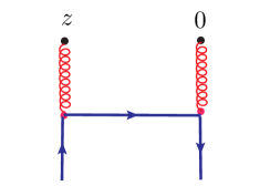
Figure 5: Gluon-quark mixing diagram.

The correction to the gluon operator with arbitrary indices generated by the gluon-quark diagram shown in Fig. 5 is presented in Appendix B. To illustrate its structure, let us take the projection corresponding to the ${\mathcal{O}}_{03}^{+}$ operator. In the $\overline{\rm MS}$ scheme, it reads

$$\frac{g^{2}C_{F}}{4\pi^{2}z_{3}} \int_{0}^{1}\differential u\left[2\bar{u}\mathcal{O}^{0}_{q}\left(uz_{3}\right)+\left.2\bar{u}uz_{3}\partial_{0}\mathcal{O}^{3}_{q}\left(uz\right)\right|_{z_{0}=0}\right]$$

$$-\frac{g^{2}C_{F}}{4\pi^{2}}\ln\left(z_{3}^{2}\mu^{2}_{IR}\frac{e^{2\gamma_{E}}}{4}\right)\int_{0}^{1}\differential u\left[(2\bar{u}u+\bar{u}^{2})\partial_{3}\mathcal{O}^{0}_{q}\left(uz_{3}\right)-(\bar{u}^{2}+u^{2})\left.\partial_{0}\mathcal{O}^{3}_{q}\left(uz\right)\right|_{z_{0}=0}\right]\ .$$ (4.5)

The singlet combination of quark fields ${\cal O}_{q}^{\mu}(z_{3})$ is defined as

$${\cal O}_{q}^{\mu}(z)=\frac{i}{2}\sum_{f}\left(\bar{\psi}_{f}(z)\gamma^{\mu}\psi_{f}(0)-\bar{\psi}_{f}(0)\gamma^{\mu}\psi_{f}(z)\right)\ ,$$ (4.6)

with $f$ numerating quark flavors. Since the matrix element of ${\cal O}_{q}^{\mu}(z)$ is odd in $z$, it can be parametrized by

$$\langle p|{\cal O}_{q}^{\mu}(z_{3})|p\rangle= 2p^{\mu}\int_{0}^{1}\differential y\sin\left(ypz\right)f_{S}(y)=-2p^{\mu}\nu\int_{0}^{1}\differential\alpha\,{\cal I}_{S}(\alpha\nu)\ ,$$ (4.7)

where $\nu=-(pz)$, as usual, and

$${\cal I}_{S}(\nu)=\int_{0}^{1}\differential y\ \cos(y\nu)\,y\,f_{S}(y)$$ (4.8)

is the singlet quark Ioffe-time distribution.

Applying this parametrization, the $gq$ correction to $M_{03}^{+}$ may be written as

$$\bra{p}G_{3i}(z)G_{i0}(0)+G_{0i}(z)G_{i3}(0)\ket{p}\quad\to-2p_{0}p_{3}\frac{g^{2}C_{F}}{4\pi^{2}}\int_{0}^{1}\differential u\,\left[\ln\left(z_{3}^{2}\mu^{2}_{IR}\frac{e^{2\gamma_{E}}}{4}\right){\cal B}_{gq}(u)+\bar{u}(1+u)\right]\mathcal{I}_{S}\left(u\nu\right)\ ,$$ (4.9)

with the $gq$ component of the evolution kernel given by ${\cal B}_{gq}(u)\equiv 1+(1-u)^{2}$. For two other matrix elements listed in Eq. (3.11), the analogs of Eq. (4.5) are given by

$$\bra{p}G_{0i}\left(z\right)G_{i0}\left(0\right)\ket{p}+\bra{p}G_{ij}\left(z\right)G_{ji}\left(0\right)\ket{p}\to-p_{0}^{2}\frac{g^{2}C_{F}}{4\pi^{2}}\ln\left(z_{3}^{2}\mu^{2}_{IR}\frac{e^{2\gamma_{E}}}{4}\right)\int_{0}^{1}\differential u\,{\cal B}_{gq}(u)\mathcal{I}_{S}\left(u\nu\right)$$ (4.10)

and

$$\bra{p}G_{3i}\left(z\right)G_{i3}\left(0\right)\ket{p}+2\bra{p}G_{30}\left(x\right)G_{03}\left(0\right)\ket{p}\quad\to-p_{0}^{2}\frac{g^{2}C_{F}}{4\pi^{2}}\int_{0}^{1}\differential u\,\left[\ln\left(z_{3}^{2}\mu^{2}_{IR}\frac{e^{2\gamma_{E}}}{4}\right){\cal B}_{gq}(u)+4\bar{u}\right]\mathcal{I}_{S}\left(u\nu\right)\ .$$ (4.11)

IV.2 Matching relations

As discussed already, the combination ${M}_{0i;i0}+{M}_{ij;ji}=2p_{0}^{2}\mathcal{M}_{pp}$, at the tree level, is proportional to the twist-2 amplitude $\mathcal{M}_{pp}$ without contaminations. The amplitude $\mathcal{M}_{pp}(\nu,z_{3}^{2})$ obtained in this way may be used to form the reduced pseudo-ITD

$${\mathfrak{M}}_{00}(\nu,z_{3}^{2})\equiv\frac{{\mathcal{M}_{pp}}(\nu,z_{3}^{2})}{{\mathcal{M}_{pp}}(0,z_{3}^{2})}\$$ (4.12)

as in Eq. (2.12). Using the results (IV), (4.10) of our calculations for the one-loop corrections to ${M}_{0i;i0}+{M}_{ij;ji}$, we obtain the matching relation

$${\mathfrak{M}}_{00}(\nu,z_{3}^{2})\,{{\cal I}_{g}(0,\mu^{2})}= {{\cal I}_{g}(\nu,\mu^{2})}$$

$$-\frac{\alpha_{s}N_{c}}{2\pi}\int_{0}^{1}\differential u\,{{\cal I}_{g}(u\nu,\mu^{2})}\Biggl{\{}\log(z_{3}^{2}\mu^{2}\frac{e^{2\gamma_{E}}}{4})\,B_{gg}(u)+4\left[\frac{u+\log(\bar{u})}{\bar{u}}\right]_{+}+\frac{2}{3}\left[1-u^{3}\right]_{+}\Biggr{\}}$$

$$-\frac{\alpha_{s}C_{F}}{2\pi}\log(z_{3}^{2}\mu^{2}\frac{e^{2\gamma_{E}}}{4})\int_{0}^{1}\differential u\,\left[{\cal I}_{S}(u\nu,\mu^{2})-{\cal I}_{S}(0,\mu^{2})\frac{{\cal I}_{g}(\nu,\mu^{2})}{{\cal I}_{g}(0,\mu^{2})}\right]\,{\cal B}_{gq}(u)\$$

$$\quad+\frac{\alpha_{s}N_{c}}{2\pi}\int_{0}^{1}\differential u\left\{{2\over 3}\left(1-u^{3}\right)+\log\left(z_{3}^{2}\mu^{2}_{\rm IR}\frac{e^{2\gamma_{E}}}{4}\right)\bar{u}\left(u^{2}+1\right)\right\}\,$$

$$\quad\times u^{2}z_{3}^{2}\left[\mathcal{M}_{ppzz}\left(u\nu,z_{3}^{2}\right)-\mathcal{M}_{ppzz}\left(0,z_{3}^{2}\right)\frac{{\cal I}_{g}(\nu,\mu^{2})}{{\cal I}_{g}(0,\mu^{2})}\right]$$ (4.13)

between the “lattice function” ${\mathfrak{M}}_{00}(\nu,z_{3}^{2})$ and the light-cone ITDs ${\cal I}_{g}(\nu,\mu^{2})$ and ${\cal I}_{S}(\nu,\mu^{2})$.

This matching condition also includes the “higher twist” term ${\cal M}_{ppzz}$ on its right-hand side. This term is accompanied by a $z_{3}^{2}$ factor that suppresses its contribution for small $z_{3}^{2}$ values, and is omitted in the matching conditions given in our original paper Balitsky et al. (2020). The size of the ${\cal M}_{ppzz}$ term may be estimated by comparing the lattice signals for ${M}_{0i;i0}+{M}_{ij;ji}$ and $M_{3i;i3}+2M_{30;03}$ matrix elements. To this end, denoting ${M_{3i;i3}(z_{3},p)+2M_{30;03}(z_{3},p)}\equiv{2p_{0}^{2}}{\mathcal{M}_{33}}(\nu,z_{3}^{2})$, we define the “33” reduced ITD,

$${\mathfrak{M}}_{33}(\nu,z_{3}^{2})\equiv\frac{{\mathcal{M}_{33}}(\nu,z_{3}^{2})}{{\mathcal{M}_{33}}(0,z_{3}^{2})}\ .$$ (4.14)

Now, using Eqs. (IV) and (4.11) we obtain the matching condition

$${\mathfrak{M}}_{33} (\nu,z_{3}^{2})\,\Big{[}{{\cal I}_{g}(0,\mu^{2})}-z_{3}^{2}\mathcal{M}_{ppzz}\left(0,z_{3}^{2}\right)\Big{]}={{\cal I}_{g}(\nu,\mu^{2})}-z_{3}^{2}\mathcal{M}_{ppzz}\left(\nu,z_{3}^{2}\right)$$

$$-\frac{\alpha_{s}N_{c}}{2\pi}\int_{0}^{1}\differential u\,\Big{[}{{\cal I}_{g}(u\nu,\mu^{2})}-u^{2}z_{3}^{2}\mathcal{M}_{ppzz}\left(u\nu,z_{3}^{2}\right)\Big{]}\Biggl{\{}\log(z_{3}^{2}\mu^{2}\frac{e^{2\gamma_{E}}}{4})\,B_{gg}(u)+4\left[\frac{u^{2}/2+\log(\bar{u})}{\bar{u}}\right]_{+}+\frac{2}{3}\left[1-u^{3}\right]_{+}\Biggr{\}}$$

$$-\frac{\alpha_{s}C_{F}}{2\pi}\int_{0}^{1}\differential u\,\left[{\cal I}_{S}(u\nu,\mu^{2})-{\cal I}_{S}(0,\mu^{2})\frac{{{\cal I}_{g}(\nu,\mu^{2})}-z_{3}^{2}\mathcal{M}_{ppzz}\left(\nu,z_{3}^{2}\right)}{{{\cal I}_{g}(0,\mu^{2})}-z_{3}^{2}\mathcal{M}_{ppzz}\left(0,z_{3}^{2}\right)}\right]\,\left\{\log(z_{3}^{2}\mu^{2}\frac{e^{2\gamma_{E}}}{4}){\cal B}_{gq}(u)+4\bar{u}\right\}\$$

$$\hskip 85.35826pt-\frac{\alpha_{s}N_{c}}{2\pi}\int_{0}^{1}\differential u\left\{2\bar{u}+\log\left(z_{3}^{2}\mu^{2}_{\rm IR}\frac{e^{2\gamma_{E}}}{4}\right)\bar{u}\left(u^{2}+1\right)\right\}\,$$

$$\hskip 85.35826pt\times u^{2}z_{3}^{2}\left[\mathcal{M}_{ppzz}\left(u\nu,z_{3}^{2}\right)-\mathcal{M}_{ppzz}\left(0,z_{3}^{2}\right)\frac{{{\cal I}_{g}(\nu,\mu^{2})}-z_{3}^{2}\mathcal{M}_{ppzz}\left(\nu,z_{3}^{2}\right)}{{{\cal I}_{g}(0,\mu^{2})}-z_{3}^{2}\mathcal{M}_{ppzz}\left(0,z_{3}^{2}\right)}\right]$$ (4.15)

that may be combined with Eq. (4.13) to estimate the impact of the $\mathcal{M}_{ppzz}$ contamination.

The gluon light-cone ITD ${\cal I}_{g}(\nu,\mu^{2})$ is related to the gluon PDF ${f}_{g}(x,\mu^{2})$ by

$${\cal I}_{g}(\nu,\mu^{2})=\frac{1}{2}\int_{-1}^{1}dx\,\,e^{ix\nu}\,x{f}_{g}(x,\mu^{2})\ .$$ (4.16)

In fact, $x{f}_{g}(x,\mu^{2})$ is an even function of $x$. Hence, the real part of ${\cal I}_{g}(\nu,\mu^{2})$ is given by the cosine transform of $x{f}_{g}(x,\mu^{2})$, while its imaginary part vanishes. The overall factor ${\cal I}_{g}(0,\mu^{2})$ corresponds to the fraction of the hadron momentum carried by the gluons, ${\cal I}_{g}(0,\mu^{2})=\langle x_{g}\rangle_{\mu^{2}}$.  This means that Eq. (4.13) allows to extract just the shape of the gluon distribution. Its normalization, i.e., the magnitude of $\langle x_{g}\rangle_{\mu^{2}}$ must be taken from an independent lattice calculation, similar to that performed in Ref. Yang et al. (2018). The singlet quark function ${\cal I}_{S}(w\nu,\mu^{2})$ that appears in the ${\cal O}(\alpha_{s})$ correction should be also calculated (or estimated) independently.

The matching condition (4.13) (without the $\mathcal{M}_{ppzz}$ terms and neglecting the gluon-quark mixing term) has been already used in lattice extractions of the unpolarized gluon PDFs by the MSU group Fan et al. (2021); Fan and Lin (2021) and the HadStruc collaboration Khan et al. (2021).

V Summary.

In this paper, we have presented the results that form the basis for the ongoing efforts to calculate gluon PDF using the pseudo-PDF approach.

In particular, we have displayed our results for the most complicated box diagram. We have presented the expression for the situation when all four indices are arbitrary, and also for combinations of indices corresponding to three matrix elements that are most convenient to extract the twist-2 invariant amplitude ${\cal M}_{pp}$. We also displayed the evolution structure for these matrix elements.

The results of our earlier publication Balitsky et al. (2020, 2021) have been already used in the lattice extractions Fan et al. (2021); Fan and Lin (2021); Khan et al. (2021) of the gluon PDF from the studies of the ${M}_{0i;i0}+{M}_{ji;ij}$ matrix element. The additional results for the box diagram and the gluon-quark contribution given in the present paper may be used for extractions of the gluon PDF from two other matrix elements, with a possible cross-check of the results obtained from different matrix elements.

Acknowledgements. We thank K. Orginos, J.-W. Qiu, D. Richards, R. Sufian, T. Khan and S. Zhao for interest in our work and discussions. This work is supported by Jefferson Science Associates, LLC under U.S. DOE Contract #DE-AC05-06OR23177 and by U.S. DOE Grant #DE-FG02-97ER41028.

Appendix A Box diagram with arbitrary indices

The full result for a forward matrix element is

$${\mathcal{O}}_{\mu\alpha;\nu\beta}^{\rm box}\to \,\frac{g^{2}N_{c}\Gamma(d/2)}{8\pi^{2}\left(-z^{2}\right)^{d/2}}\int_{0}^{1}\differential u\left(z_{\mu}z_{\nu}g_{\alpha\beta}-z_{\alpha}z_{\nu}g_{\mu\beta}-z_{\mu}z_{\beta}g_{\alpha\nu}+z_{\alpha}z_{\beta}g_{\mu\nu}\right)\frac{2\bar{u}^{3}}{3}G_{z\xi}(uz)G_{z}^{\ \xi}(0)$$

$$+\frac{g^{2}N_{c}\Gamma(d/2-1)}{8\pi^{2}\left(-z^{2}\right)^{d/2-1}}\int_{0}^{1}\differential u\left\{\vphantom{\frac{1}{2}}\left(g_{\alpha\beta}g_{\mu\nu}-g_{\mu\beta}g_{\nu\alpha}\right)\frac{2\bar{u}^{3}}{3}G_{z\xi}(uz)G_{z}^{\ \xi}(0)\right.$$

$$\left.+\frac{\bar{u}^{3}}{3}\left(g_{\alpha\beta}G_{z\nu}(uz)G_{z\mu}(0)-g_{\mu\beta}G_{z\nu}(uz)G_{z\alpha}(0)-g_{\alpha\nu}G_{z\beta}(uz)G_{z\mu}(0)+g_{\mu\nu}G_{z\beta}(uz)G_{z\alpha}(0)\right)\right.$$

$$\left.+(2u\bar{u}+\frac{\bar{u}^{3}}{3})\left(g_{\alpha\beta}G_{z\mu}(uz)G_{z\nu}(0)-g_{\mu\beta}G_{z\alpha}(uz)G_{z\nu}(0)-g_{\alpha\nu}G_{z\mu}(uz)G_{z\beta}(0)+g_{\mu\nu}G_{z\alpha}(uz)G_{z\beta}(0)\right)\right.$$

$$+\bar{u}^{2}\left(\vphantom{\frac{1}{2}}\right.z_{\nu}G_{\alpha\beta}(uz)G_{z\mu}(0)-z_{\nu}G_{\mu\beta}(uz)G_{z\alpha}(0)-z_{\beta}G_{\alpha\nu}(uz)G_{z\mu}(0)+z_{\beta}G_{\mu\nu}(uz)G_{z\alpha}(0)$$

$$-z_{\mu}G_{z\nu}(uz)G_{\alpha\beta}(0)+z_{\alpha}G_{z\nu}(uz)G_{\mu\beta}(0)+z_{\mu}G_{z\beta}(uz)G_{\alpha\nu}(0)-z_{\alpha}G_{z\beta}(uz)G_{\mu\nu}(0)\left.\vphantom{\frac{1}{2}}\right)$$

$$+\bar{u}(1+u)\left(\vphantom{\frac{1}{2}}\right.z_{\nu}G_{z\mu}(uz)G_{\alpha\beta}(0)-z_{\nu}G_{z\alpha}(uz)G_{\mu\beta}(0)-z_{\beta}G_{z\mu}(uz)G_{\alpha\nu}(0)+z_{\beta}G_{z\alpha}(uz)G_{\mu\nu}(0)$$

$$-z_{\mu}G_{\alpha\beta}(uz)G_{z\nu}(0)+z_{\alpha}G_{\mu\beta}(uz)G_{z\nu}(0)+z_{\mu}G_{\alpha\nu}(uz)G_{z\beta}(0)-z_{\alpha}G_{\mu\nu}(uz)G_{z\beta}(0)\left.\vphantom{\frac{1}{2}}\right)$$

$$+(\frac{\bar{u}^{2}}{2}-\frac{\bar{u}^{3}}{3})\left(\vphantom{\frac{1}{2}}\right.z_{\nu}g_{\alpha\beta}G_{\mu\xi}(uz)G_{z}^{\ \xi}(0)-z_{\nu}g_{\mu\beta}G_{\alpha\xi}(uz)G_{z}^{\ \xi}(0)-z_{\beta}g_{\alpha\nu}G_{\mu\xi}(uz)G_{z}^{\ \xi}(0)+z_{\beta}g_{\mu\nu}G_{\alpha\xi}(uz)G_{z}^{\ \xi}(0)$$

$$+z_{\nu}g_{\alpha\beta}G_{z\xi}(uz)G_{\mu}^{\ \xi}(0)-z_{\nu}g_{\mu\beta}G_{z\xi}(uz)G_{\alpha}^{\ \xi}(0)-z_{\beta}g_{\alpha\nu}G_{z\xi}(uz)G_{\mu}^{\ \xi}(0)+z_{\beta}g_{\mu\nu}G_{z\xi}(uz)G_{\alpha}^{\ \xi}(0)$$

$$+z_{\mu}g_{\alpha\beta}G_{\nu\xi}(uz)G_{z}^{\ \xi}(0)-z_{\alpha}g_{\mu\beta}G_{\nu\xi}(uz)G_{z}^{\ \xi}(0)-z_{\mu}g_{\alpha\nu}G_{\beta\xi}(uz)G_{z}^{\ \xi}(0)+z_{\alpha}g_{\mu\nu}G_{\beta\xi}(uz)G_{z}^{\ \xi}(0)$$

$$+z_{\mu}g_{\alpha\beta}G_{z\xi}(uz)G_{\nu}^{\ \xi}(0)-z_{\alpha}g_{\mu\beta}G_{z\xi}(uz)G_{\nu}^{\ \xi}(0)-z_{\mu}g_{\alpha\nu}G_{z\xi}(uz)G_{\beta}^{\ \xi}(0)+z_{\alpha}g_{\mu\nu}G_{z\xi}(uz)G_{\beta}^{\ \xi}(0)\left.\vphantom{\frac{1}{2}}\right)$$

$$+2\bar{u}\left(z_{\mu}z_{\nu}G_{\alpha\xi}(uz)G_{\beta}^{\ \xi}(0)-z_{\alpha}z_{\nu}G_{\mu\xi}(uz)G_{\beta}^{\ \xi}(0)-z_{\mu}z_{\beta}G_{\alpha\xi}(uz)G_{\nu}^{\ \xi}(0)+z_{\alpha}z_{\beta}G_{\mu\xi}(uz)G_{\nu}^{\ \xi}(0)\right)$$

$$\left.-\frac{\bar{u}^{3}}{6}\left(z_{\mu}z_{\nu}g_{\alpha\beta}-z_{\alpha}z_{\nu}g_{\mu\beta}-z_{\mu}z_{\beta}g_{\alpha\nu}+z_{\alpha}z_{\beta}g_{\mu\nu}\right)G_{\zeta\xi}(uz)G^{\zeta\xi}(0)\right\}$$

$$+\frac{g^{2}N_{c}\Gamma(d/2-2)}{8\pi^{2}\left(-z^{2}\right)^{d/2-2}}\int_{0}^{1}\differential u\left\{\vphantom{\frac{1}{2}}\right.-\bar{u}\left(G_{\alpha\beta}(uz)G_{\mu\nu}(0)-G_{\mu\beta}(uz)G_{\alpha\nu}(0)-G_{\alpha\nu}(uz)G_{\mu\beta}(0)+G_{\mu\nu}(uz)G_{\alpha\beta}(0)\right)$$

$$-2uG_{\mu\alpha}(uz)G_{\nu\beta}(0)+\bar{u}(1-2u)G_{\nu\beta}(uz)G_{\mu\alpha}(0)+\bar{u}(1+2u)G_{\mu\alpha}(uz)G_{\nu\beta}(0)$$

$$+\frac{\bar{u}u^{2}}{2}\left(g_{\alpha\beta}G_{\mu\xi}(uz)G_{\nu}^{\ \xi}(0)-g_{\mu\beta}G_{\alpha\xi}(uz)G_{\nu}^{\ \xi}(0)-g_{\alpha\nu}G_{\mu\xi}(uz)G_{\beta}^{\ \xi}(0)+g_{\mu\nu}G_{\alpha\xi}(uz)G_{\beta}^{\ \xi}(0)\right)$$

$$+\frac{\bar{u}u^{2}}{2}\left(g_{\alpha\beta}G_{\nu\xi}(uz)G_{\mu}^{\ \xi}(0)-g_{\mu\beta}G_{\nu\xi}(uz)G_{\alpha}^{\ \xi}(0)-g_{\alpha\nu}G_{\beta\xi}(uz)G_{\mu}^{\ \xi}(0)+g_{\mu\nu}G_{\beta\xi}(uz)G_{\alpha}^{\ \xi}(0)\right)$$

$$+\bar{u}\left(g_{\mu\nu}G_{\alpha\xi}(uz)G_{\beta}^{\ \xi}(0)-g_{\alpha\nu}G_{\mu\xi}(uz)G_{\beta}^{\ \xi}(0)-g_{\mu\beta}G_{\alpha\xi}(uz)G_{\nu}^{\ \xi}(0)+g_{\alpha\beta}G_{\mu\xi}(uz)G_{\nu}^{\ \xi}(0)\right)$$

$$-\left(g_{\mu\nu}g_{\alpha\beta}-g_{\nu\alpha}g_{\mu\beta}\right)\frac{\bar{u}^{3}}{6}G_{\zeta\xi}(uz)G^{\zeta\xi}(0)\left.\vphantom{\frac{1}{2}}\right\}\ .\hskip 241.84842pt{\rm(A.1)}$$

Appendix B Gluon-quark contribution with arbitrary indices

$$iG_{\mu\alpha}\left(z\right)G_{\nu\beta}\left(0\right)\to \frac{g^{2}C_{F}\Gamma(d/2)z_{\mu}z_{\nu}}{8\pi^{2}\left(-z^{2}\right)^{d/2}}\int_{0}^{1}\differential u\bar{u}\bar{\psi}_{c}(uz)\left[-g_{\alpha\beta}z_{\eta}\gamma^{\eta}-i\epsilon_{\alpha z\beta\eta}\gamma^{\eta}\gamma_{5}\right]\psi_{c}(0)$$

$$+\frac{g^{2}C_{F}\Gamma(d/2-1)}{16\pi^{2}\left(-z^{2}\right)^{d/2-1}}\int_{0}^{1}\differential u\left\{\vphantom{1\over}g_{\mu\nu}\bar{u}\bar{\psi}_{c}(uz)\left[\left(z_{\alpha}g_{\beta\eta}+z_{\beta}g_{\alpha\eta}-g_{\alpha\beta}z_{\eta}\right)\gamma^{\eta}-i\epsilon_{\alpha z\beta\eta}\gamma^{\eta}\gamma_{5}\right]\psi_{c}(0)\right.$$

$$\left.+z_{\nu}\left(\vphantom{1\over}\bar{u}u\bar{\psi}_{c}(uz)\overleftarrow{\partial}_{\mu}\left[\left(z_{\alpha}g_{\beta\eta}-g_{\alpha\beta}z_{\eta}\right)\gamma^{\eta}-i\epsilon_{\alpha z\beta\eta}\gamma^{\eta}\gamma_{5}\right]\psi_{c}(0)\right.\right.$$

$$\left.\left.+\bar{u}\bar{\psi}_{c}(uz)\left[\left(g_{\mu\beta}g_{\alpha\eta}-g_{\alpha\beta}g_{\mu\eta}\right)\gamma^{\eta}-i\epsilon_{\alpha\mu\beta\eta}\gamma^{\eta}\gamma_{5}\right]\psi_{c}(0)\vphantom{1\over}\right)\right.$$

$$\left.+z_{\mu}\left(\vphantom{1\over}\bar{u}u\bar{\psi}_{c}(uz)\overleftarrow{\partial}_{\nu}\left[\left(z_{\beta}g_{\alpha\eta}-g_{\alpha\beta}z_{\eta}\right)\gamma^{\eta}-i\epsilon_{\alpha z\beta\eta}\gamma^{\eta}\gamma_{5}\right]\psi_{c}(0)\right.\right.$$

$$\left.\left.+\bar{u}\bar{\psi}_{c}(uz)\left[\left(g_{\alpha\nu}g_{\beta\eta}-g_{\alpha\beta}g_{\nu\eta}\right)\gamma^{\eta}-i\epsilon_{\alpha\nu\beta\eta}\gamma^{\eta}\gamma_{5}\right]\psi_{c}(0)\vphantom{1\over}\right)\right.$$

$$\left.-z_{\mu}z_{\nu}\bar{u}^{2}\left[\bar{\psi}_{c}(uz)\left(\overleftarrow{\partial}_{\alpha}\gamma_{\beta}+\gamma_{\alpha}\overleftarrow{\partial}_{\beta}\right)\psi_{c}(0)\right]\vphantom{1\over}\right\}$$

$$+\frac{g^{2}C_{F}\Gamma(d/2-2)}{32\pi^{2}\left(-z^{2}\right)^{d/2-2}}\int_{0}^{1}\differential u\left\{\vphantom{1\over}-g_{\mu\nu}\bar{u}^{2}\bar{\psi}_{c}(uz)\left(\overleftarrow{\partial}_{\alpha}\gamma_{\beta}+\gamma_{\alpha}\overleftarrow{\partial}_{\beta}\right)\psi_{c}(0)\right.$$

$$\left.+\bar{u}u^{2}\bar{\psi}_{c}(uz)\overleftarrow{\partial}_{\nu}\overleftarrow{\partial}_{\mu}\left[\left(z_{\alpha}g_{\beta\eta}+z_{\beta}g_{\alpha\eta}-g_{\alpha\beta}z_{\eta}\right)\gamma^{\eta}-i\epsilon_{\alpha z\beta\eta}\gamma^{\eta}\gamma_{5}\right]\psi_{c}(0)\right.$$

$$\left.+\bar{u}u\bar{\psi}_{c}(uz)\overleftarrow{\partial}_{\nu}\left[\left(g_{\mu\beta}g_{\alpha\eta}-g_{\alpha\beta}g_{\mu\eta}\right)\gamma^{\eta}-i\epsilon_{\alpha\mu\beta\eta}\gamma^{\eta}\gamma_{5}\right]\psi_{c}(0)\right.$$

$$\left.+\bar{u}u\bar{\psi}_{c}(uz)\overleftarrow{\partial}_{\mu}\left[\left(g_{\alpha\nu}g_{\beta\eta}-g_{\alpha\beta}g_{\nu\eta}\right)\gamma^{\eta}-i\epsilon_{\alpha\nu\beta\eta}\gamma^{\eta}\gamma_{5}\right]\psi_{c}(0)\right.$$

$$\left.-u\bar{u}^{2}z_{\nu}\partial_{\mu}\partial_{\beta}\bar{\psi}_{c}(uz)\gamma_{\alpha}\psi_{c}(0)-u\bar{u}^{2}z_{\mu}\partial_{\nu}\partial_{\alpha}\bar{\psi}_{c}(uz)\gamma_{\beta}\psi_{c}(0)\vphantom{1\over}\right\}$$

$$-h.c.-\left\{\mu\leftrightarrow\alpha\right\}-\left\{\nu\leftrightarrow\beta\right\}+\left\{\mu\leftrightarrow\alpha,\nu\leftrightarrow\beta\right\}\hskip 184.9429pt{\rm(B.1)}$$

References

- Constantinou et al. (2021) M. Constantinou et al., Prog. Part. Nucl. Phys. 121, 103908 (2021), arXiv:2006.08636 [hep-ph] .
- Cichy and Constantinou (2019) K. Cichy and M. Constantinou, Adv. High Energy Phys. 2019, 3036904 (2019), arXiv:1811.07248 [hep-lat] .
- Ji (2013) X. Ji, Phys. Rev. Lett. 110, 262002 (2013), arXiv:1305.1539 [hep-ph] .
- Ji (2014) X. Ji, Sci. China Phys. Mech. Astron. 57, 1407 (2014), arXiv:1404.6680 [hep-ph] .
- Ma and Qiu (2018a) Y.-Q. Ma and J.-W. Qiu, Phys. Rev. D 98, 074021 (2018a), arXiv:1404.6860 [hep-ph] .
- Ma and Qiu (2018b) Y.-Q. Ma and J.-W. Qiu, Phys. Rev. Lett. 120, 022003 (2018b), arXiv:1709.03018 [hep-ph] .
- Braun and Müller (2008) V. Braun and D. Müller, Eur. Phys. J. C 55, 349 (2008), arXiv:0709.1348 [hep-ph] .
- Bali et al. (2018a) G. S. Bali et al., Eur. Phys. J. C 78, 217 (2018a), arXiv:1709.04325 [hep-lat] .
- Bali et al. (2018b) G. S. Bali, V. M. Braun, B. Gläßle, M. Göckeler, M. Gruber, F. Hutzler, P. Korcyl, A. Schäfer, P. Wein, and J.-H. Zhang, Phys. Rev. D 98, 094507 (2018b), arXiv:1807.06671 [hep-lat] .
- Radyushkin (2017a) A. V. Radyushkin, Phys. Rev. D 96, 034025 (2017a), arXiv:1705.01488 [hep-ph] .
- Radyushkin (2017b) A. Radyushkin, PoS QCDEV2017, 021 (2017b), arXiv:1711.06031 [hep-ph] .
- Orginos et al. (2017) K. Orginos, A. Radyushkin, J. Karpie, and S. Zafeiropoulos, Phys. Rev. D 96, 094503 (2017), arXiv:1706.05373 [hep-ph] .
- Xiong et al. (2014) X. Xiong, X. Ji, J.-H. Zhang, and Y. Zhao, Phys. Rev. D 90, 014051 (2014), arXiv:1310.7471 [hep-ph] .
- Ji and Zhang (2015) X. Ji and J.-H. Zhang, Phys. Rev. D 92, 034006 (2015), arXiv:1505.07699 [hep-ph] .
- Izubuchi et al. (2018) T. Izubuchi, X. Ji, L. Jin, I. W. Stewart, and Y. Zhao, Phys. Rev. D 98, 056004 (2018), arXiv:1801.03917 [hep-ph] .
- Wang and Zhao (2018) W. Wang and S. Zhao, JHEP 05, 142 (2018), arXiv:1712.09247 [hep-ph] .
- Wang et al. (2018) W. Wang, S. Zhao, and R. Zhu, Eur. Phys. J. C 78, 147 (2018), arXiv:1708.02458 [hep-ph] .
- Wang et al. (2019) W. Wang, J.-H. Zhang, S. Zhao, and R. Zhu, Phys. Rev. D 100, 074509 (2019), arXiv:1904.00978 [hep-ph] .
- Ji et al. (2015) X. Ji, A. Schäfer, X. Xiong, and J.-H. Zhang, Phys. Rev. D 92, 014039 (2015), arXiv:1506.00248 [hep-ph] .
- Xiong and Zhang (2015) X. Xiong and J.-H. Zhang, Phys. Rev. D 92, 054037 (2015), arXiv:1509.08016 [hep-ph] .
- Liu et al. (2019) Y.-S. Liu, W. Wang, J. Xu, Q.-A. Zhang, J.-H. Zhang, S. Zhao, and Y. Zhao, Phys. Rev. D 100, 034006 (2019), arXiv:1902.00307 [hep-ph] .
- Ji et al. (2017) X. Ji, J.-H. Zhang, and Y. Zhao, Nucl. Phys. B 924, 366 (2017), arXiv:1706.07416 [hep-ph] .
- Radyushkin (2018a) A. V. Radyushkin, Phys. Lett. B 781, 433 (2018a), arXiv:1710.08813 [hep-ph] .
- Radyushkin (2018b) A. Radyushkin, Phys. Rev. D 98, 014019 (2018b), arXiv:1801.02427 [hep-ph] .
- Zhang et al. (2018) J.-H. Zhang, J.-W. Chen, and C. Monahan, Phys. Rev. D 97, 074508 (2018), arXiv:1801.03023 [hep-ph] .
- Radyushkin (2019) A. V. Radyushkin, Phys. Rev. D 100, 116011 (2019), arXiv:1909.08474 [hep-ph] .
- Balitsky et al. (2020) I. Balitsky, W. Morris, and A. Radyushkin, Phys. Lett. B 808, 135621 (2020), arXiv:1910.13963 [hep-ph] .
- Balitsky et al. (2021) I. Balitsky, W. Morris, and A. Radyushkin, in 28th International Workshop on Deep Inelastic Scattering and Related Subjects (2021) arXiv:2106.01916 [hep-ph] .
- Fan et al. (2021) Z. Fan, R. Zhang, and H.-W. Lin, Int. J. Mod. Phys. A 36, 2150080 (2021), arXiv:2007.16113 [hep-lat] .
- Fan and Lin (2021) Z. Fan and H.-W. Lin, (2021), arXiv:2110.14471 [hep-lat] .
- Khan et al. (2021) T. Khan et al. (HadStruc), Phys. Rev. D 104, 094516 (2021), arXiv:2107.08960 [hep-lat] .
- Ioffe (1969) B. L. Ioffe, Phys. Lett. B 30, 123 (1969).
- Li et al. (2019) Z.-Y. Li, Y.-Q. Ma, and J.-W. Qiu, Phys. Rev. Lett. 122, 062002 (2019), arXiv:1809.01836 [hep-ph] .
- Zhang et al. (2019) J.-H. Zhang, X. Ji, A. Schäfer, W. Wang, and S. Zhao, Phys. Rev. Lett. 122, 142001 (2019), arXiv:1808.10824 [hep-ph] .
- Chen et al. (2017) J.-W. Chen, X. Ji, and J.-H. Zhang, Nucl. Phys. B 915, 1 (2017), arXiv:1609.08102 [hep-ph] .
- Balitsky and Braun (1989) I. I. Balitsky and V. M. Braun, Nucl. Phys. B 311, 541 (1989).
- Yang et al. (2018) Y.-B. Yang, M. Gong, J. Liang, H.-W. Lin, K.-F. Liu, D. Pefkou, and P. Shanahan, Phys. Rev. D 98, 074506 (2018), arXiv:1805.00531 [hep-lat] .