A Minimax Learning Approach to Off-Policy Evaluation in Confounded Partially Observable Markov Decision Processes

Abstract

We consider off-policy evaluation (OPE) in Partially Observable Markov Decision Processes (POMDPs), where the evaluation policy depends only on observable variables and the behavior policy depends on unobservable latent variables. Existing works either assume no unmeasured confounders, or focus on settings where both the observation and the state spaces are tabular. In this work, we first propose novel identification methods for OPE in POMDPs with latent confounders, by introducing bridge functions that link the target policy’s value and the observed data distribution. We next propose minimax estimation methods for learning these bridge functions, and construct three estimators based on these estimated bridge functions, corresponding to a value function-based estimator, a marginalized importance sampling estimator, and a doubly-robust estimator. Our proposal permits general function approximation and is thus applicable to settings with continuous or large observation/state spaces. The nonasymptotic and asymptotic properties of the proposed estimators are investigated in detail. A Python implementation of our proposal is available at https://github.com/jiaweihhuang/Confounded-POMDP-Exp.

1 Introduction

Reinforcement learning (RL) has been successfully applied in online settings (e.g., video games) where interaction with environments is easy and the data can be adaptively generated. However, online interaction is often costly and dangerous for a number of high-stake domains ranging from health science to social science and economics. Offline (batch) reinforcement learning is concerned with policy learning and evaluation with limited and pre-collected data in a sample efficient manner Levine et al. (2020). The focus of this paper is the off-policy evaluation (OPE) problem, which refers to the task of estimating the value of an evaluation policy offline using data collected under a different behavior policy. It is critical in sequential decision-making problems from healthcare, robotics, and education where new policies need to be evaluated offline before online validation.

There is a growing literature on OPE (see e.g., Precup, 2000; Jiang and Li, 2016; Thomas and Brunskill, 2016; Liu et al., 2018; Xie et al., 2019; Yin and Wang, 2020; Liao et al., 2020; Yang et al., 2020; Pananjady and Wainwright, 2021; Kuzborskij et al., 2021; Zhang et al., 2021; Shi et al., 2021). A common assumption made in the aforementioned works is that of no unmeasured confounders. Specifically, they assume the time-varying state variables are fully observed and no unmeasured variables exist that confound the observed actions. However, this assumption is not testable from the data. It is often violated in observational datasets generated from healthcare applications.

To allow unmeasured confounders to exist, we model the observed data by a Partially Observable Markov Decision Process (POMDP). Under this framework, the behavior policy is allowed to depend on some unobserved state variables that confound the action-reward association. The goal of OPE in POMDPs is to estimate the value of an evaluation policy, which is a function of observed variables, using the data generated by such a behavior policy. This is a highly challenging problem. Directly applying the importance sampling methods Precup (2000); Liu et al. (2018) or the value function-based method Munos and Szepesvári (2008) would yield a biased estimator, as we do not have access to the unobserved state variables. Tennenholtz et al. (2020); Nair and Jiang (2021) have made important progresses on this problem by outlining a consistent OPE estimator in tabular settings. However, they are not applicable to settings with continuous observation/state spaces.

In this paper, we study OPE in non-tabular POMDPs. Our contributions are summarized as follows. First, we provide a novel identification method for OPE with latent confounders. We only require the existence of two bridge functions, corresponding to a weight bridge function and a value bridge function. These bridge functions are defined as solutions to some integral equations. They can be interpreted as projections of the marginalized importance sampling weight and value functions defined on the latent state space onto the observation space. They are not always uniquely defined, but we do not require the uniqueness assumption to achieve consistent estimation.

Second, we propose minimax learning methods to estimate the two bridge functions with function approximation. The proposed method allows us to model these bridge functions via certain highly flexible function approximators (e.g., neural networks) and is thus applicable to settings with continuous or large observation/state spaces. Based on the estimated bridge functions, we further propose three estimators for the target policy’s value, corresponding to a value function-based estimator, a marginalized importance sampling (IS) estimator and a doubly-robust (DR) estimator.

Finally, we systematically study the nonasymptotic and asymptotic properties of the proposed estimators. Specifically, we first show the finite-sample rate of convergence under the realizability and Bellman closedness assumptions on value bridge function. Similar assumptions are imposed on the Q- or density ratio function in fully observable MDP settings Munos and Szepesvári (2008); Uehara et al. (2021). Second, when the realizability assumption holds for both bridge functions, we establish the finite-sample rate of convergence of the proposed estimators without assuming Bellman closedness. Finally, when the bridge functions are uniquely defined, we prove that the DR estimator is asymptotically normal and achieves the Cramér-Rao lower bound. We expect our findings to contribute to the theoretical understanding of offline RL (see e.g., Munos and Szepesvári, 2008; Chen and Jiang, 2019; Kallus and Uehara, 2019).

1.1 Related Works

We discuss some related works on OPE with unmeasured confounders and spectral learning in this section. To save space, some additional related works on minimax estimation and negative controls are discussed in Appendix A.

OPE with Unmeasured Confounders

To handle unmeasured confounders, existing OPE methods can be roughly divided into the following three categories. The first type of methods proposes to develop partial identification bounds for the policy value based on sensitivity analysis Kallus and Zhou (2020); Namkoong et al. (2020); Zhang and Bareinboim (2021). These methods rely on certain assumptions that might be difficult to validate in practice. For instance, Kallus and Zhou (2020) imposes a memoryless unmeasured confounding assumption.

The second type of methods derive the value estimates by making use of some auxiliary variables in the observed data (Zhang and Bareinboim, 2016; Futoma et al., 2020; Wang et al., 2020; Bennett et al., 2021; Liao et al., 2021; Ying et al., 2021; Shi et al., 2022). These methods are not directly applicable to the POMDP setting we consider. For instance, Zhang and Bareinboim (2016); Wang et al. (2020); Liao et al. (2021); Shi et al. (2022) propose to model the observed data via a confounded MDP. In these settings, the time-varying observations satisfy the Markov property. However, the Markov assumption is violated in POMDPs.

The third type of methods adopt the POMDP model to formulate the confounded OPE problem and develop value estimators in tabular settings (Tennenholtz et al., 2020; Nair and Jiang, 2021). However, as we have commented, these methods are ineffective in non-tabular settings with continuous or large observation/state spaces.

Spectral learning in POMDPs

Our proposal is closely related to a line of works on developing spectral learning methods in the POMDP literature (Song et al., 2010; Boots et al., 2011; Hsu et al., 2012; Anandkumar et al., 2014; Hefny et al., 2015; Kulesza et al., 2015; Jin et al., 2020). These methods are originally designed for learning system dynamics in the absence of unmeasured confounders. They would yield biased value estimators in the presence of unmeasured confounders.

2 Problem Formulation

We consider a discounted Partially Observable Markov Decision Process (POMDP) defined as

$$\langle{\mathcal{S}},\mathcal{A},\mathcal{O},\{r_{t}\}_{t\geq 0},\{P_{t}\}_{t\geq 0},\{Z_{t}\}_{t\geq 0},\gamma\rangle,$$

where ${\mathcal{S}}$ denotes the state space, $\mathcal{A}$ denotes the finite action space, $\mathcal{O}$ denotes the observation space, $P_{t}:{\mathcal{S}}\times\mathcal{A}\to\Delta({\mathcal{S}})$ denotes the state transition kernel at time $t$, $Z_{t}:{\mathcal{S}}\to\Delta(\mathcal{O})$ denotes the observation function that defines the conditional distribution of the observation given the state at time $t$, $r_{t}:{\mathcal{S}}\times\mathcal{A}\to\mathbb{R}$ denotes a bounded reward function that depends on the state-action pair at time $t$, and $\gamma\in[0,1)$ is a discount factor that balances the immediate and future rewards. $P_{t},r_{t}$ and $Z_{t}$ are unknown to us and need to be inferred from the observed data.

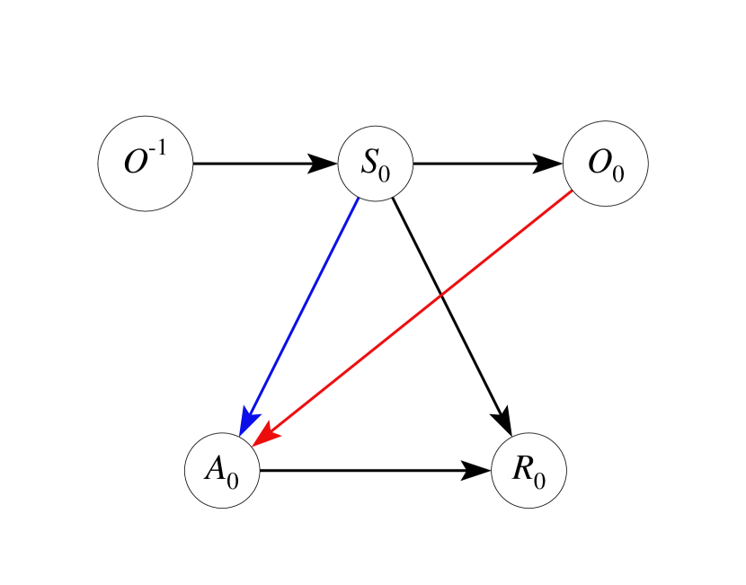
The data generating process in POMDPs is depicted in Figure 1. Suppose the environment is in a given state $s\in{\mathcal{S}}$. The agent selects an action $a\in\mathcal{A}$. Then the system transits into a new state $s^{\prime}$ and gives an immediate reward $r(s,a)$ to the agent. While we cannot directly observe the latent state $s$, we have access to an observation $o\sim Z(\cdot|s)$. This model is adopted from Tennenholtz et al. (2020) where the observation does not depend on the previous action. Nonetheless, one may define a new state/observation vector by concatenating the current state/observation and the past action. The resulting formulation is reduced to the general POMDP setup. A policy is a set of time-dependent decision rules $\pi=\{\pi_{t}\}$ where each $\pi_{t}:{\mathcal{S}}\times\mathcal{O}\to\Delta(\mathcal{A})$ maps the state-observation pair to a probability distribution over the action space. For a given policy $\pi$, the data generating process can be summarized as $S_{0}\sim\nu_{0},O_{0}\sim Z_{0}(\cdot|S_{0}),A_{0}\sim\pi_{0}(\cdot|S_{0},O_{0}),R_{0}=r_{0}(S_{0},A_{0}),S_{1}\sim P_{0}(\cdot|S_{0},A_{0}),\cdots$ where $\nu_{0}$ denotes the initial state distribution. The observed data up to $t$ is given by $\tau_{t}=(O_{0},A_{0},R_{0},\cdots,O_{t},A_{t},R_{t})$. We denote its distribution by $P_{\pi}$. The policy value $J(\pi)$ is defined as the expected cumulative reward $\mathbb{E}_{\pi}[\sum_{t=0}^{H}\gamma^{t}R_{t}]$ for some $0<H\leq+\infty$, where the expectation is taken w.r.t. the distribution of trajectories induced by policy $\pi$.

For a given evaluation policy $\pi^{e}=\{\pi^{e}_{t}\}_{t}$, the goal of OPE is to estimate $J(\pi^{e})$ from an observational dataset generated by a behavior policy $\pi^{b}=\{\pi^{b}_{t}\}_{t}$. Similar to Tennenholtz et al. (2020), we focus on the setting where $\pi^{b}$ depends only on the latent state and $\pi^{e}$ depends only on the observation. See also Figure 1. Under this model assumption, the state variables serve as a confounder between the action and the reward at each time. Since the state is not fully observed, the no unmeasured confounder assumption is violated.

$\varepsilon$	True Value	Ours	Naive
0.25	4.94	5.01	7.0
0.5	4.99	5.008	5.004
0.75	5.03	5.07	3.008

Table 1: The proposed OPE estimator and the naive IS or value function-based estimator which replaces the state with the observation when applied to the toy data example with 1e4 trajectories and 100 times points per trajectory. The naive IS and value function-based estimator are computed via minimax weight and Q-function learning (Uehara et al., 2020), respectively. The two estimators are the same under the tabular setting and are denoted by “Naive”.

Finally, we illustrate the challenge of OPE with latent confounders. If we were to observe the latent state, following the standard OPE methods, we could identify the policy value using the marginalized IS or the value function-based estimator. However, since we cannot observe the state, these methods are not applicable. Naively replacing the state with the observation would yield biased estimators.

To elaborate, we design a toy example with binary observation, state, and action spaces. Specifically, the target policy is a uniform random policy and the behavior policy is given by $\pi_{t}^{b}(1|1)=\pi_{t}^{b}(0|0)=1-\varepsilon$, for some constant $0<\varepsilon<1$ and any $t\geq 0$. When $\varepsilon=0.5$, the action is independent of the latent state and no unmeasured confounders exist. The naive IS or value function-based estimator which replaces the state with the observation is expected to be consistent in that case. We report the true value (computed via the Monte-Carlo method), our proposed value estimator and the naive estimator when applied to a large dataset with 1e4 trajectories and 100 time points per trajectory in Table 1. It can be seen that the naive method works only when $\varepsilon=0.5$, as expected. In contrast, the proposed estimator is consistent in all cases.

3 Partially Observable Contextual Bandits

As a warm-up, we start with a partially observable contextual bandit setting (a special case of POMDP with horizon that equals 1) to present our main idea. Suppose we have $N$ data tuples that are i.i.d. $\{O_{-1},A_{0},O_{0},R_{0}\}$ tuples where $O_{-1}$ denotes the additional observation that is conditionally independent of $(A_{0},O_{0},R_{0})$ given $S_{0}$. The corresponding Bayesian network is depicted in Figure 2(a).

Figure 1: The data generating process in POMDPs. The evaluation policy in red depends on the observed variables. The behavior policy depends on the hidden state variables.

The IS and value-function based estimators are given by

$$\textstyle\mathbb{E}\left[\eta_{0}(S_{0},A_{0})R_{0}\right],\mathbb{E}\left[v_{0}(S_{0})\right]=\sum_{a}\mathbb{E}q_{0}(S_{0},a)\pi^{e}_{0}(a\mid S_{0}),$$

respectively, where $q_{0}(S_{0},A_{0})=\mathbb{E}[R_{0}\mid S_{0},A_{0}]$, $\eta_{0}=\pi^{e}_{0}/\pi^{b}_{0}$ denotes the IS ratio, $\sum_{a}$ is an abbreviation of $\sum_{a\in\mathcal{A}}$, and the expectation $\mathbb{E}$ without any subscript is taken w.r.t. to the distribution of the offline data. As we have commented, these methods are not applicable since $S_{0}$ is unobserved.

To handle unmeasured confounders, we first assume the existence of certain bridge functions that link the target policy’s value and the observed data distribution.

Assumption 1 (Existence of bridge functions).

There exist functions $b^{\prime}_{V}:\mathcal{A}\times\mathcal{O}\to\mathbb{R},b^{\prime}_{W}:\mathcal{A}\times\mathcal{O}\to\mathbb{R}$ that satisfy

$$\mathbb{E}[b^{\prime}_{V}(A_{0},O_{0})\mid S_{0},A_{0}]=\mathbb{E}[R_{0}\pi_{0}^{e}(A_{0}\mid O_{0})\mid A_{0},S_{0}],$$ (1)

$$\mathbb{E}[b^{\prime}_{W}(A_{0},O_{-1})\mid S_{0},A_{0}]=1/\pi_{0}^{b}(A_{0}\mid S_{0}).$$ (2)

We refer to $b^{\prime}_{V}(\cdot)$ as a value bridge function and $b^{\prime}_{W}(\cdot)$ as a weight bridge function.

By definition, weight bridge and value bridge functions can be interpreted as projections of the importance sampling weight (i.e., inverse propensity score) and value functions defined on the latent state space onto the observation space. It is worthwhile to mention that we do not require these bridge functions to be uniquely defined. When ${\mathcal{S}}$ and $\mathcal{O}$ are discrete, the existence of solutions to the integral equations in (1) and (2) is equivalent to certain matrix rank assumptions; see the assumptions in Nair and Jiang (2021); Boots et al. (2011); Hsu et al. (2012). These assumptions require observed variables to contain sufficient information about unobserved states. Specifically, define a matrix $\Omega_{a}=\mathrm{Pr}_{\pi^{b}}(\mathbf{O}_{0}|A_{0}=a,\mathbf{O}_{-1})$ whose $(i,j)$-th element is given by $\mathrm{Pr}_{\pi^{b}}(\mathbf{O}_{0}=o_{i}|A_{0}=a,\mathbf{O}_{-1}=o_{j})$ where $o_{i}$ denotes the $i$th element in the observation space. Then they require ${\rm rank}(\Omega_{a})=|{\mathcal{S}}|$ for any $a\in\mathcal{A}$. See Appendix B for details. When ${\mathcal{S}}$ and $\mathcal{O}$ are continuous, it follows from Picard’s theorem that Assumption 1 is implied by several conditions (Carrasco et al., 2007, Theorem 2.41). Here, we remark the value bridge function is target policy dependent and it might be more appropriate to write $b_{V}^{\prime}$ as $b_{V^{\prime}}^{\pi^{e}}$. Nonetheless, to ease the notation, we will remove the superscript $\pi^{e}$ throughout the paper.

Next, we show that Assumption 1 is a sufficient condition for policy value identification. The following theorem shows that if we know $b^{\prime}_{V}$ and $b^{\prime}_{W}$ in advance, we can consistently estimate the target value $J(\pi^{e})$ from the offline data.

Lemma 1 (Pseudo identification formula).

Suppose Assumption 1 holds. Then, for any $b^{\prime}_{V},b^{\prime}_{W}$ that solve (1),

$$\begin{split}J(\pi^{e})=\mathbb{E}\left[\sum_{a}b^{\prime}_{V}(a,O_{0})\right]\quad\hbox{and}\\ J(\pi^{e})=\mathbb{E}[b^{\prime}_{W}(A_{0},O_{-1})R_{0}\pi^{e}_{0}(A_{0}\mid O_{0})].\end{split}$$ (3)

These formulas outline an IS estimator and a value function-based estimator for $J(\pi^{e})$. It remains to identify the bridge functions $b_{V}^{\prime}$ and $b_{W}^{\prime}$. However, even if Assumption 1 holds, it is still very challenging to learn $b_{V}^{\prime}$ and $b_{W}^{\prime}$ from the observed data as their definitions involve the unobserved state $S_{0}$. As such, we refer to Lemma 1 as the “pseudo” identification formula. In the following, we introduce some versions of bridge functions that are identifiable from the observed data.

Definition 1 (Learnable bridge functions).

The learnable value bridge function $b_{V}:\mathcal{A}\times\mathcal{O}\to\mathbb{R}$ and learnable weight bridge function $b_{W}:\mathcal{A}\times\mathcal{O}\to\mathbb{R}$ are solutions to

$$\begin{split}\mathbb{E}[R_{0}\pi^{e}_{0}(A_{0}|O_{0})|A_{0},O_{-1}]=\mathbb{E}[b_{V}(A_{0},O_{0})|A_{0},O_{-1}]\\ \hbox{and}\quad 1/P_{\pi^{b}}(A_{0}|O_{0})=\mathbb{E}[b_{W}(A_{0},O_{-1})|A_{0},O_{0}].\end{split}$$ (4)

Throughout this paper, we use $b^{\prime}$ to denote a bridge function and $b$ to denote a learnable bridge function. The following lemma shows that any bridge function is a learnable bridge function.

Lemma 2.

Bridge functions defined as solutions to (1) and (2) are learnable bridge functions.

We next present an equivalent definition for $b_{W}$. This characterization is useful when extending our results to the POMDP setting.

Lemma 3.

$\mathbb{E}[b_{W}(A_{0},O_{-1})\mid A_{0},O_{0}]=1/P_{\pi^{b}}(A_{0}\mid O_{0})$ holds if and only if

$$\mathbb{E}[\sum_{a}f(O_{0},a)-b_{W}(A_{0},O_{-1})f(O_{0},A_{0})]=0,\quad\forall f.$$

As we have commented, the class of bridge functions are difficult to estimate from the observed data. On the other hand, the class of learnable bridge functions is identifiable. However, they are not necessarily bridge functions. Thus, we cannot invoke Lemma 1 for value identification. Nonetheless, perhaps surprisingly, the following theorem shows that we can plug-in any learnable bridge function $b_{V}$ and $b_{W}$ for $b_{V}^{\prime}$ and $b_{W}^{\prime}$ in (3) under Assumption 1.

Theorem 1 (Key identification formula).

Assume the existence of value bridge functions and learnable weight bridge functions. Then, letting $b_{W}(\cdot)$ be a learnable weight bridge function, we have

$$J(\pi^{e})=\mathbb{E}[b_{W}(A_{0},O_{-1})R_{0}].$$

Suppose the existence of weight bridge functions and learnable value bridge functions. Then, letting $b_{V}(\cdot)$ be a learnable value bridge function, we have

$$J(\pi^{e})=\mathbb{E}[\sum_{a}b_{V}(a,O_{0})].$$

We make a few remarks. First, the assumptions in the first and second statements do not imply each other. In both cases, Assumption 1, the existence of bridge functions, plays a critical role in ensuring the validity of the above equations. Specifically, when Assumption 1 holds, the assumptions in both the first and second statements are automatically satisfied, since bridge functions are learnable bridge functions. If we naively replace Assumption 1 with the existence of learnable bridge functions that satisfy equation 2, then Theorem 1 is no longer valid.

Second, Theorem 1 implies that we only need bridge functions to exist, but do not need to identify them. As long as they exist, learnable bridge functions can be used for estimation, which are not necessarily bridge functions.

(a) Partially Observable Contextual Bandits

(b) Time-homogeneous POMDPs.

Figure 2: Red lines depict the dependency of evaluation policies on the observed variables. Blue lines depict the dependence of behavior policies on the state variables.

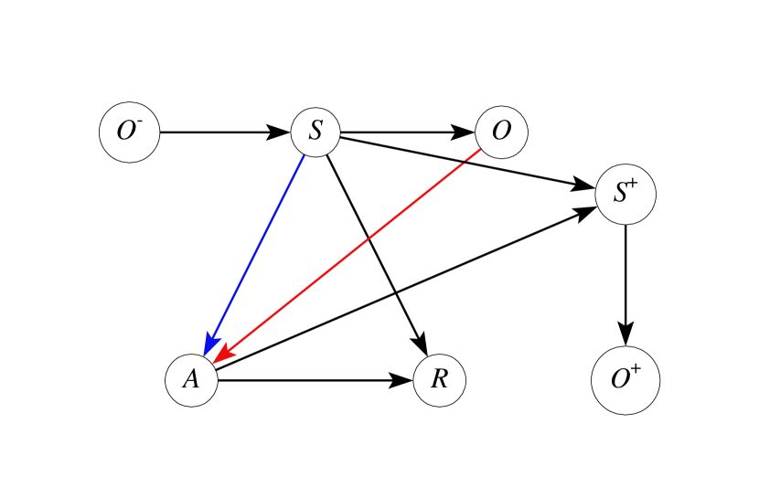
Third, similar identification methods have been developed in the causal inference literature for evaluating the average treatment effect with double negative controls; see Appendix A. However, their settings differ from ours. For instance, those works require policies to be constant functions of negative controls. In contrast, we allow our evaluation policy to depend on the observation which serves as negative controls in their setting.

Finally, Theorem 1 requires the existence of both the value and the (learnable) weight bridge functions. Under certain completeness assumptions, $J(\pi^{e})$ can be uniquely identified by assuming the existence of value bridge functions only, and the discussion is deferred to the end of Section 4.1.

4 OPE in Time-homogeneous POMDPs

In this section, we focus on time-homogeneous POMDPs where $P_{t},Z_{t},r_{t},\pi^{e}_{t},\pi^{b}_{t}$ are stationary over time. We denote them by $P,Z,r,\pi^{e},\pi^{b}$, respectively. OPE in time-inhomogeneous POMDPs is investigated in Appendices 5 and 6. Our goal is to estimate the target policy’s value in the infinite horizon setting ($H=\infty$). Consider a data tuple $(O^{-},S,O,A,R,S^{+},O^{+})$ following

$$(O^{-},S)\sim P_{\pi^{b}}(\cdot),A\sim\pi^{b}(\cdot|S),S^{+}\sim P(\cdot|S,A),$$

$$R=r(S,A),O^{+}\sim Z(\cdot|S^{+}),$$

where $P_{\pi^{b}}$ denotes certain distribution over $\mathcal{O}\times{\mathcal{S}}$. The observed data tuple is given by $(O^{-},O,A,R,O^{+})$. For example, for a data trajectory $\{(O_{t},A_{t},R_{t})\}_{0\leq t\leq n+1}$ under $\pi_{b}$, the observations can be summarized as $\{(O_{t-1},O_{t},A_{t},R_{t},O_{t+1})\}_{1\leq t\leq n}$. The above configuration is satisfied with $P_{\pi^{b}}$ equal to the occupancy distribution under $\pi_{b}$ over $\mathcal{O}\times{\mathcal{S}}$. This conversion from trajectories to tuples is commonly used in the offline RL literature (Chen and Jiang, 2019). We assume the initial observation distribution $\nu_{\mathcal{O}}(o)\coloneqq\int Z(o\mid s)\nu(s){\textnormal{d}}(s)$ is known to us. If unknown, it can be estimated by the empirical data distribution. With a slight abuse of notation, we denote the distribution of the data as $P_{\pi^{b}}(\cdot)$, e.g., $P_{\pi^{b}}(a\mid s)=\pi^{b}(a\mid s)$. In addition, $P_{\pi^{b}}(s)$ denote the probability mass function (or the probability density function) when the state is discrete (or continuous).

4.1 Identification

First, we extend our definitions of the bridge functions to the POMDP setting and require their existence in the assumption below. Let $w(s)=\sum_{t\geq 0}\gamma^{t}P_{\pi^{e},t}(s)/P_{\pi^{b}}(s)$ denote the marginal density ratio where $P_{\pi^{e},t}(\cdot)$ denotes the probability density function of $S_{t}$ under the evaluation policy. In addition, let $q^{\pi^{e}}(a,s)=\mathbb{E}_{\pi^{e}}[\sum_{t\geq 0}\gamma^{t}R_{t}|A_{0}=a,S_{0}=s]$ denote the Q-function. These functions play an important role in constructing marginalized IS and value function-based estimators in fully observable MDPs. The following bridge functions play similar roles in POMDPs.

Assumption 2 (Existence of bridge functions).

There exist value bridge functions $b^{\prime}_{V}:\mathcal{A}\times\mathcal{O}\to\mathbb{R}$ and weight bridge functions $b^{\prime}_{W}:\mathcal{A}\times\mathcal{O}\to\mathbb{R}$ that satisfy

$$\mathbb{E}[b^{\prime}_{V}(A_{0},O_{0})\mid A_{0},S_{0}] =\mathbb{E}_{\pi^{e}}[\sum_{t}\gamma^{t}R_{t}\pi^{e}(A_{0}\mid O_{0})|A_{0},S_{0}],$$

$$\mathbb{E}[b^{\prime}_{W}(A,O^{-})\mid A,S] =\frac{w(S)}{\pi^{b}(A|S)}.$$

We make several remarks. First, the existence of $b^{\prime}_{W}$ implicitly requires $\pi^{b}(a|s)>0$ and $w(s)<\infty$ for any $a$ and $s$. The latter condition is weaker than requiring $P_{\pi^{b}}(s)>0$ for any $s$. In other words, we do not require the full coverage assumption. Second, when the states are fully observed and ${\mathcal{S}}=\mathcal{O}$, it follows immediately that $b^{\prime}_{V}(a,s)=q^{\pi^{e}}(a,s)\pi^{e}(a\mid s)$ and $b^{\prime}_{W}(a,s)=w(s)/\pi^{b}(a\mid s)$. Similar to the bandit setting, these bridge functions can thus be interpreted as projections of the value functions and the marginalized IS weights onto the the observation space. Third, we do not require the bridge functions to be uniquely defined.

Next, we define the learnable bridge functions. They are consistent with those in Definition 1 when $\gamma=0$.

Definition 2 (Learnable bridge functions).

Learnable value bridge functions $b_{V}$ are defined as solutions to

$$\begin{split}\mathbb{E}[b_{V}(A,O)\mid A,O^{-}]=\mathbb{E}[R\pi^{e}(A\mid O)\mid A,O^{-}]\\ +\gamma\mathbb{E}\left[\sum_{a^{\prime}}b_{V}(a^{\prime},O^{+})\pi^{e}(A\mid O)\mid A,O^{-}\right].\end{split}$$ (5)

Learnable weight bridge functions $b_{W}$ are defined as solutions to

$$\mathbb{E}[L_{\mathbb{W}}(b_{W},f)]=0,\quad\forall f:\mathcal{O}\times\mathcal{A}\to\mathbb{R}$$ (6)

where $L_{\mathbb{W}}(g,f)$ equals

$$\sum_{a^{\prime}}\gamma g(A,O^{-})\pi^{e}(A|O)f(O^{+},a^{\prime})-g(A,O^{-})f(O,A)$$

$$+(1-\gamma)\mathbb{E}_{\tilde{O}\sim\nu_{\mathcal{O}}}[\sum_{a^{\prime}}f(\tilde{O},a^{\prime})].$$

Finally, we show our key identification formula under Assumption 2. It extends Lemma 2 and Theorem 1 to the POMDP setting.

Theorem 2 (Key identification theorem).

1. Any bridge function is a learnable bridge function.

2. Suppose the existence of the value bridge function and learnable weight bridge function $b_{W}(\cdot)$. Then,

   $$J(\pi^{e})=\frac{1}{1-\gamma}\mathbb{E}[b_{W}(A,O^{-})R\pi^{e}(A\mid O)].$$

3. Suppose the existence of the weight bridge function and learnable value bridge function $b_{V}(\cdot)$. Then,

   $$J(\pi^{e})=\mathbb{E}_{\tilde{O}\sim\nu_{\mathcal{O}}}[\sum_{a}b_{V}(a,\tilde{O})].$$

Similar to the bandit setting, any bridge function is a learnable bridge function, but the reverse is not true. However, the target policy’s value can be consistently estimated based on any learnable bridge function. In addition, similar to the bandit setting, the existence is equivalent to the rank assumption ${\rm rank}(\mathrm{Pr}_{\pi^{b}}(\mathbf{O}_{0}\mid a,\mathbf{O}^{-}))=|{\mathcal{S}}|$ in tabular case.

Theorem 2 forms the basis of our estimation procedure. It outlines a marginalized IS estimator and a value function-based estimator for policy evaluation. We remark that conditions in bullet points 2 and 3 do not imply each other. In addition, when Assumption 2 holds, conditions in 2 and 3 are automatically satisfied.

To identify policy values, we have so far imposed the following assumptions: (a) learnable value bridge functions exist and weight bridge functions exist; (b) learnable weight functions exist and value bridge functions exist. In this section, we show that the policy value can also be identified with the existence of the learnable value bridge functions only. However, in that case, we would need to impose some completeness conditions. We summarize the results in the following theorem.

Theorem 3 (Identification with completeness).

Suppose a learnable value bridge function $b_{V}$ exists, and a completeness assumption holds:

$$\mathbb{E}[g(S,A)\mid A,O^{-}]=0\implies g(S,A)=0.$$

Then, we have $J(\pi^{e})=\mathbb{E}_{\tilde{o}\sim\nu_{\mathcal{O}}}[\sum_{a}b_{V}(a,\tilde{o})].$

Compared to Theorem 2, the existence of weight bridge functions is replaced with the completeness assumption.

4.2 Estimation

We first propose three value estimators given certain consistently estimated learnable bridge functions $\hat{b}_{V}$ and $\hat{b}_{W}$. We next introduce minimax estimation methods for $b_{V}$ and $b_{W}$.

Given some $\hat{b}_{V}$ and $\hat{b}_{W}$, we can construct the following IS and value function-based estimators accordingly to Theorem 2. Specifically, define $\hat{J}_{\mathrm{IS}}$ and $\hat{J}_{\mathrm{VM}}$ to be

$$\frac{1}{1-\gamma}\mathbb{E}_{\mathcal{D}}[\hat{b}_{W}(A,O^{-})R\pi^{e}(A\mid O)]\,\,\hbox{and}\,\,\mathbb{E}_{\tilde{O}\sim\nu_{\mathcal{O}}}[\sum_{a}\hat{b}_{V}(a,\tilde{O})],$$

respectively, where $\mathbb{E}_{\mathcal{D}}$ denotes the empirical average over all observed data tuples.

In addition, we can combine the aforementioned two estimators for policy evaluation. This yields the following doubly-robust estimator, $\hat{J}_{\mathrm{DR}}=\mathbb{E}_{\mathcal{D}}[J(\hat{b}_{W},\hat{b}_{V})]$ where

$$\begin{split}J(f,g)\coloneqq\mathbb{E}_{\tilde{O}\sim\nu_{\mathcal{O}}}[\sum_{a}g(a,\tilde{O})]+\frac{f(A,O^{-})}{1-\gamma}\\ \times\Big{[}\{R+\gamma\sum_{a^{\prime}}g(a^{\prime},O^{+})\}\pi^{e}(A\mid O)-g(A,O)\Big{]},\end{split}$$ (7)

for $f:\mathcal{A}\times\mathcal{O}\to\mathbb{R}$ and $g:\mathcal{A}\times\mathcal{O}\to\mathbb{R}$. It has the desired doubly-robust property, as shown in Section 4.3.2.

In fully observable MDPs, $\hat{J}_{\mathrm{IS}}$ reduces to the marginalized IS estimator Liu et al. (2018), and $\hat{J}_{\mathrm{DR}}$ reduces to the doubly-robust estimator (Kallus and Uehara, 2019). We remark that our proposal is not a trivial extension of these existing methods to the POMDP setting. The major challenge lies in developing identification formulas in Theorem 2 to correctly identify the target policy’s value. These results are not needed in settings without unmeasured confounders.

Next, we present our proposal to estimate $b_{V}$ and $b_{W}$. To estimate $b_{V}$, a key observation is that, it satisfies the following integral equation, $\mathbb{E}[L_{\mathbb{V}}(b_{V},f)]=0$ for any $f$ where $L_{\mathbb{V}}(g,f)$ is given by

$$[\{R+\gamma\sum_{a^{\prime}}g(a^{\prime},O^{+})\}\pi^{e}(A|O)-g(A,O)]f(A,O^{-}).$$

This motivates us to develop the following minimax learning methods. Specifically, we begin with two function classes $\mathcal{V},\mathcal{V}^{\dagger}\subset\{\mathcal{A}\times\mathcal{O}\to\mathbb{R}\}$ and a regularization parameter $\lambda\in\mathbb{R}^{+}$. We next define the following minimax estimator,

$$\hat{b}_{V}=\operatorname*{arg\,min}_{g\in\mathcal{V}}\max_{f\in\mathcal{V}^{\dagger}}\mathbb{E}_{\mathcal{D}}[L_{\mathbb{V}}(g,f)]-\lambda\mathbb{E}_{\mathcal{D}}[f^{2}].$$ (8)

Here, we use the function class $\mathcal{V}$ to model the oracle value bridge function, and the function class $\mathcal{V}^{\dagger}$ to measure the discrepancy between a given $g\in\mathcal{V}$ and the oracle learnable value bridge function. In practice, we can use linear basis functions, neural networks, random forests, reproducing kernel Hilbert spaces (RKHSs), etc., to parameterize these functions. In the fully observable MDP setting, the above optimization reduces to Modified Bellman Residual Minimization (MBRM) when $\lambda=0.5$ Antos et al. (2008) and Minimax Q-learning (MQL) when $\lambda=0$ Uehara et al. (2020). It is worthwhile to mention that fitted Q-iteration (FQI, Ernst et al., 2005), a popular policy learning method in MDPs, cannot be straightforwardly extended to the POMDP setting. This is because the regression estimator in each iteration of FQI will be biased under the POMDP setting.

Similarly, according to (6), we consider the following estimator for the weight bridge function,

$$\hat{b}_{W}=\operatorname*{arg\,min}_{g\in\mathcal{W}}\max_{f\in\mathcal{W}^{\dagger}}\mathbb{E}_{\mathcal{D}}[L_{\mathbb{W}}(g,f)]-\lambda\mathbb{E}_{\mathcal{D}}[f^{2}],$$ (9)

for some function classes $\mathcal{W},\mathcal{W}^{\dagger}\subset\{\mathcal{A}\times\mathcal{O}\to\mathbb{R}\}$ and some $\lambda\in\mathbb{R}^{+}$.

In practice, we recommend to use linear models or RKHSs to parametrize $V^{\dagger}$ and $\mathcal{W}^{\dagger}$. This allows us to get the closed-form expression for the inner maximization. To the contrary, $\mathcal{V}$ and $\mathcal{W}$ can be parametrized by any function classes such as neural networks. When $\mathcal{V}$ and $\mathcal{W}$ are linear models or RKHSs as well, we can obtain the complete closed-form solution for $\hat{b}_{W}$. We discuss this further in Appendix C.

4.3 Theoretical Results for Minimax Estimators

We first investigate the nonasymptotic properties of the value function-based estimator $\hat{J}_{\mathrm{VM}}$. We next study the asymptotic property of the DR estimator $\hat{J}_{\mathrm{DR}}$. Results of the importance sampling estimator can be similarly derived. We discuss this in Appendix C. Our results extend some recently established OPE theories in MDPs (Munos and Szepesvári, 2008; Chen and Jiang, 2019; Kallus and Uehara, 2019; Uehara et al., 2021) to the POMDP setting. We assume the observed dataset $\mathcal{D}$ consist of $n$ i.i.d. copies of $(O^{-},O,A,R,O^{+})$. This i.i.d. assumption is commonly employed in the RL literature to simplify the proof (see e.g., Dai et al., 2020).

4.3.1 Value function-based methods

We begin with the value function-based estimator. First, to measure the discrepancy between the estimated learnable value bridge function $\hat{b}_{V}$ and $b_{V}$, we introduce the Bellman residual error for POMDPs as follows:

Definition 3.

The Bellman residual operator ${\mathcal{T}}$maps a given function $f:\mathcal{A}\times\mathcal{O}\to\mathbb{R}$ to another function ${\mathcal{T}}f$such that

$${\mathcal{T}}f(a,o)=\mathbb{E}[R\pi^{e}(A\mid O)+\gamma\sum_{a^{\prime}}f(a^{\prime},O^{+})\pi^{e}(A\mid O)$$

$$-f(A,O)\mid A=a,O^{-}=o],\quad\forall a,o.$$

The bellman residual error is defined as $\mathbb{E}[\{{\mathcal{T}}f(A,O^{-})\}^{2}]$.

By definition, the Bellman residual error is zero for any learnable bridge function. As such, it quantifies how a given function $f$ deviates from the oracle value bridge functions. In MDPs, it reduces to the standard Bellman residual error.

We next establish the rate of convergence of $\hat{b}_{V}$ in the following theorem.

Theorem 4 (Convergence rate of $\hat{b}_{V}$).

Set $\lambda>0$ in Equation 8. Suppose (a) there exists certain learnable bridge function that satisfies Equation 5; (b) $\mathcal{V}$ and $\mathcal{V}^{\dagger}$ are finite hypothesis classes; (c) $\mathcal{V}$ contains at least one learnable bridge function; (d) ${\mathcal{T}}\mathcal{V}\subset\mathcal{V}^{\dagger}$; (e) There exist some constants $C_{\mathcal{V}}$ and $C_{\mathcal{V}^{\dagger}}$ such that $\forall v\in\mathcal{V},\|v\|_{\infty}\leq C_{\mathcal{V}}$ and $\forall v\in\mathcal{V}^{\dagger},\|v\|_{\infty}\leq C_{\mathcal{V}^{\dagger}}$ Then, there exists some universal constant $c>0$ such that for any $\delta>0$, with probability $1-\delta$, $\mathbb{E}[\{{\mathcal{T}}\hat{b}_{V}(A,O^{-})\}^{2}]^{1/2}$ is upper bounded by

$$c\max(1,C_{\mathcal{V}},C_{\mathcal{V}^{\dagger}})\sqrt{\log(|\mathcal{V}||\mathcal{V}^{\dagger}|c/\delta)/n}.$$

It is important to note we only assume the existence of the learnable value bridge function in (a). We do not impose any assumptions on weight bridge functions. Assumption (b) can be further relaxed by assuming that $\mathcal{V}$ and $\mathcal{V}^{\dagger}$ are general hypothesis classes. In that case, the convergence rate will be characterized by the critical radii of function classes constructed by $\mathcal{V}$ and $\mathcal{V}^{\dagger}$. See e.g., Uehara et al. (2021) for details. Assumption (c) is the realizability assumption. Since learnable bridge functions are not unique, we only require $\mathcal{V}$ to contain one of them. Assumption (d) is the (Bellman) closedness assumption. It requires that the discriminator class $\mathcal{V}^{\dagger}$ is sufficiently rich and the operator $\mathcal{B}$ is sufficiently smooth. These assumptions are valid in several examples, including tabular and linear models. To save space, we relegate the related discussions to Appendix C.

Next, we derive the convergence guarantee of the policy value estimator.

Theorem 5 (Convergence rate of $\hat{J}_{\mathrm{VM}}$).

Suppose the weight bridge functions $b^{\prime}_{W}(\cdot)$ and learnable value bridge functions exist, and Assumption (a)-(e) in Theorem 4 hold. Then, there exists some universal constant $c>0$ such that for any $\delta>0$, with probability $1-\delta$, $|J(\pi^{e})-\hat{J}_{\mathrm{VM}}|$ is upper bounded by

$$\textstyle\frac{c}{1-\gamma}\{\max(1,C_{\mathcal{V}},C_{\mathcal{V}^{\dagger}})\mathbb{E}[b^{\prime 2}_{W}(A,O^{-})]\}^{\frac{1}{2}}\sqrt{\frac{\log(|\mathcal{V}||\mathcal{V}^{\dagger}|c/\delta)}{n}}.$$

Theorem 5 requires a stronger condition than Theorem 4, as we assume the existence of weight bridge function. Its proof relies on the following key equation,

$$|J(\pi^{e})-\hat{J}_{\mathrm{VM}}|\leq\mathbb{E}[b^{\prime 2}_{W}(A,O^{-})]^{1/2}\mathbb{E}[\{{\mathcal{T}}\hat{b}_{V}(A,O^{-})\}^{2}]^{1/2},$$

where the upper bound for the second term on the right-hand-side is given in Theorem 4.

Notice that Theorem 4 relies on the closedness assumption, e.g., Assumption (d). We remark that this condition is not necessary to derive the convergence rate of the final policy value estimator. In Theorem 14 (see Appendix C), we show that when $b_{V}\in\mathcal{V},b_{W}\in\mathcal{V}^{\dagger}$, similar results can be established without any closedness conditions.

4.3.2 DR methods

We focus on the DR estimator in this section. We first establish its doubly-robustness property in Theorem 6. It implies that as long as either $\hat{b}_{W}$ or $\hat{b}_{V}$ is consistent, the final estimator $\hat{J}_{\mathrm{DR}}$ is consistent.

Theorem 6 (Doubly-robustness property).

Suppose Assumption 2 holds. Then $J(f,g)$ defined in Equation 7 equals $J(\pi^{e})$ as long as either $f=b_{W}$ or $g=b_{V}$.

We next show that $\hat{J}_{\mathrm{DR}}$ is efficient in the sense that it is asymptotically normal with asymptotic variance equal to the Cramér-Rao Lower Bound.

First, we provide the Cramér-Rao Lower Bound. To simplify the technical proof, we focus on the tabular setting. Nonetheless, we conjecture that the same result still holds in the non-tabular setting as well. We leave further investigation of this conjecture to future work.

Theorem 7.

Suppose ${\mathcal{S}},\mathcal{A},\mathcal{O}$ are finite discrete spaces. Assume ${\rm rank}(\operatorname{Pr}_{\pi^{b}}(\mathbf{O}\mid A=a,\mathbf{O}^{-}))=|{\mathcal{S}}|=|\mathcal{O}|$. The Cramér-Rao Lower Bound is given by

$$V_{\mathrm{EIF}} =\mathbb{E}[J(b_{W},b_{V})^{2}].$$

We impose a rank assumption in Theorem 7. This condition implies that the bridge functions are uniquely defined, and so are the learnable bridge functions. We remark that without such a uniqueness assumption, the Cramér-Rao Lower Bound is not well-defined.

Next, we analyze the property of DR estimator. To avoid imposing certain Donsker conditions (van der Vaart, 1998), we focus on a sample-split version of $\hat{J}_{\mathrm{DR}}$ as in Zheng and van der Laan (2011). It splits all data trajectories in $\mathcal{D}$ into two independent subsets $\mathcal{D}_{1},\mathcal{D}_{2}$, computes the estimated bridge function $\hat{b}^{(1)}_{V},\hat{b}^{(1)}_{W}$ ($\hat{b}^{(2)}_{V},\hat{b}^{(2)}_{W}$) based on the data subset in $\mathcal{D}_{2}$ ($\mathcal{D}_{1}$), and does the estimation of the value based on the remaining dataset. Finally, we aggregate the resulting two estimates to get full efficiency. This yields the following DR estimator,

$$\hat{J}^{*}_{\mathrm{DR}}=0.5\mathbb{E}_{\mathcal{D}_{1}}[J(\hat{b}^{(1)}_{W},\hat{b}^{(1)}_{V})]+0.5\mathbb{E}_{\mathcal{D}_{2}}[J(\hat{b}^{(2)}_{W},\hat{b}^{(2)}_{V})].$$

We summarize the results in the following theorem. Notice that they are valid in the non-tabular setting as well.

Theorem 8.

Assume the existence and uniqueness of bridge and learnable bridge functions. Suppose $\hat{b}_{W},b_{W},\hat{b}_{V},b_{V}$ are uniformly bounded by some constants, $\mathbb{E}[\{\hat{b}^{(j)}_{W}-b_{W}\}^{2}(A,O^{-})]=o_{p}(1),\mathbb{E}[\{{\mathcal{T}}\hat{b}^{(j)}_{V}(A,O^{-})\}^{2}]=o_{p}(1),\\ \mathbb{E}[\{\sum_{a}\hat{b}^{(j)}_{V}(a,O)-b_{V}(a,O)\}^{2}]^{1/2}=o_{p}(1),\mathbb{E}[\{\hat{b}^{(j)}_{W}-b_{W}\}^{2}(A,O^{-})]^{1/2}\mathbb{E}[\{{\mathcal{T}}\hat{b}^{(j)}_{V}(A,O^{-})\}^{2}]^{1/2}=o_{p}(n^{-1/2})$ for $j=1,2$. Then, $\sqrt{n}(\hat{J}^{*}_{\mathrm{DR}}-J(\pi^{e}))$ weakly converges to a normal distribution with mean 0 and variance $V_{\mathrm{EIF}}$.

We again, make a few remarks. First, although the estimated bridge functions are required to satisfy certain nonparametric rates only, the resulting value estimator achieves a parametric rate of convergence (e.g. $n^{-1/2}$). This is essentially due to the doubly-robustness property, which ensures that the bias of the estimator can be represented as a product of the difference between the two estimated bridge functions and their oracle values. Second, Theorem 8 derives the asymptotic variance of $\hat{J}^{*}_{\mathrm{DR}}$, which can be consistently estimated from the data. This allows us to perform a handy Wald-type hypothesis testing. Finally, Theorem 8 requires a stronger assumption, i.e., the uniqueness of bridge functions, which implies that $|{\mathcal{S}}|=|\mathcal{O}|$. Without this assumption, it remains unclear how to define the $L_{2}$ error of the estimated bridge function. However, we would like to remark that imposing the uniqueness condition is not a weakness of our analysis, but the CR lower bound statement we hope to prove does not make sense if the condition fails.

5 OPE in Time-inhomogeneous POMDPs

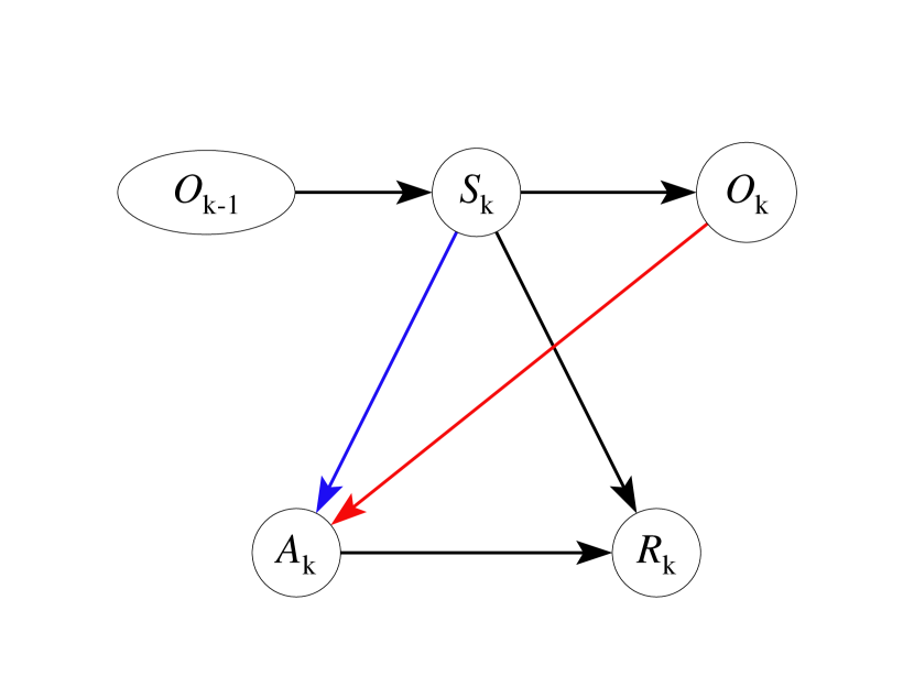
We consider the time-inhomogeneous setting in this section where the system dynamics, evaluation and behavior policies are allowed to vary over time. We first introduce the identification method for the target policy’s value by introducing value and weight bridge functions. We next present the proposed value function-based, IS and DR estimators. We remark that although we focus on evaluation of Markovian policies in this section, the proposed value function-based estimator can be extended to settings where evaluation policies are history-dependent in Section 6.

(a) The case where we use the prior observation as a negative control.

(b) The case where we use the prior history as a negative control.

5.1 Identification

We first introduce the bridge function and the learnable bridge function. For any $j\geq 1$, Let $\mu_{j}(s_{j})=\frac{P_{\pi^{e},j}(s_{j})}{P_{\pi^{b},j}(s_{j})}$ where $P_{\pi^{e},j}$ and $P_{\pi^{b},j}$ are the marginal density functions of $S_{j}$ under $\pi^{e}$ and $\pi^{b}$, respectively. Let $\mathfrak{J}_{j-1}=\{O_{0},A_{0},O_{1},A_{1},R_{1},O_{2},\cdots,R_{j-1}\}$.

Assumption 3 (Existence of bridge functions).

There exist value bridge functions $\{b^{\prime[j]}_{V}\}_{j=0}^{H-1}$ and weight bridge functions $\{b^{\prime[j]}_{W}\}_{j=0}^{H-1}$, defined as solutions to

$$\mathbb{E}[b^{\prime[j]}_{V}(A_{j},O_{j})\mid A_{j},S_{j}] =\mathbb{E}_{\pi^{e}}[\sum_{t=j}^{H-1}\gamma^{t-j}R_{t}\pi^{e}_{j}(A_{j}\mid{O_{j}})|A_{j},S_{j}],$$ (10)

$$\mathbb{E}[b^{\prime j}_{W}(A_{j},\mathfrak{J}_{j-1})\mid A_{j},S_{j}] =\mu_{j}(S_{j})\frac{1}{P_{\pi^{b}}(A_{j}\mid S_{j})}.$$ (11)

Definition 4 (Learnable bridge functions).

Learnable value bridge functions $\{b^{[j]}_{V}\}_{j=0}^{H-1}$ and learnable weight bridge functions $\{b^{[j]}_{W}\}_{j=0}^{H-1}$ are defined as solutions to

$$\begin{split}&\mathbb{E}[b^{[j]}_{V}(A_{j},O_{{j}})\mid A_{j},\mathfrak{J}_{j-1}]=\mathbb{E}[R_{j}\pi^{e}_{j}(A_{j}\mid{O_{j}})+\gamma\sum_{a^{\prime}}b^{[j+1]}_{V}(a^{\prime},{O_{j+1}})\pi^{e}_{j}(A_{j}\mid{O_{j}})\mid A_{j},\mathfrak{J}_{j-1}],\\ &\mathbb{E}\left[\sum_{a^{\prime}}b^{[j]}_{W}(A_{j},\mathfrak{J}_{j-1})\pi^{e}_{j}(A_{j}|O_{j})f({O_{j+1}},a^{\prime})-b^{[j+1]}_{W}(A_{j+1},{\mathfrak{J}_{j}})f({O_{j+1}},A_{j+1})\right]=0,\,\forall f:\mathcal{A}\times\mathcal{O}\to\mathbb{R}.\end{split}$$ (12)

It is important to note that we use the whole history $\mathfrak{J}_{j-1}$ in the integral equations to define the learnable bridge functions. Alternatively, one can replace $\mathfrak{J}_{j-1}$ with the most recent observation $O_{j-1}$. The advantage of using the whole history over a single observation is that it requires weaker assumptions to ensure the existence of the bridge functions. See the discussion below Assumption 4 for details.

Next, we present our key identification theorem under Assumption 3.

Theorem 9.

Suppose Assumption 3 holds. Then, bridge functions are learnable bridge functions. In addition, any learnable bridge function satisfies

$$J(\pi^{e})=\mathbb{E}[\sum_{a}b^{[0]}_{V}(a,O_{0})],\quad J(\pi^{e})=\mathbb{E}[\sum_{t=0}^{H-1}b^{[t]}_{W}(A_{t},\mathfrak{J}_{t-1})\pi^{e}_{t}(A_{t}\mid O_{t})\gamma^{t}R_{t}].$$

The next theorem states we can similarly identify the policy value by assuming the completeness.

Theorem 10.

Suppose the existence of leanrbale value bridge functions and the completeness:

$$\mathbb{E}[g(S_{j},A_{j})\mid A_{j},\mathfrak{J}_{j-1}]=0\implies g()=0.$$

Then, any learnable bridge function satisfies

$$J(\pi^{e})=\mathbb{E}[\sum_{a}b^{[0]}_{V}(a,O_{0})].$$

To further elaborate Assumptions in Theorem 9 and Theorem 10, we focus on the tabular setting in the rest of this section when ${\mathcal{S}},\mathcal{O}$, and the reward space are discrete.

First, we see sufficient conditions to ensure Assumptions in Theorem 9. Assumptions in Theorem 9, i.e., Assumption 3, are immediately implied by the following conditions.

Assumption 4.

For any $0\leq j\leq H-1$,

$${\rm rank}(\operatorname{Pr}(\mathbf{O}_{j}\mid\mathbf{S}_{j}))=|{\mathcal{S}}|,\quad{\rm rank}(\operatorname{Pr}(\mathbfcal{J}_{j-1}\mid\mathbf{S}_{j}))=|{\mathcal{S}}|.$$

Next, we see sufficient conditions to ensure Assumption in Theorem 10. Assumptions in Theorem 10 are immediately implied by the following conditions.

Assumption 5.

For any $0\leq j\leq H-1$,

$${\rm rank}(\operatorname{Pr}(\mathbf{O}_{j}\mid\mathbf{S}_{j}))=|{\mathcal{S}}|,\quad{\rm rank}(\operatorname{Pr}(\mathbf{S}_{j}\mid\mathbfcal{J}_{j-1},A_{j}=a))=|{\mathcal{S}}|.$$

These assumptions imply that the state space is sufficiently informative and $|\mathcal{O}|\geq|{\mathcal{S}}|$. Clearly, this shows the advantage of using the whole $\mathbfcal{J}_{j-1}$ as a negative control rather than $O_{j-1}$ itself since ${\rm rank}(\operatorname{Pr}(\mathbfcal{J}_{j-1}\mid\mathbf{S}_{j}))=|{\mathcal{S}}|$ is weaker than ${\rm rank}(\operatorname{Pr}(\mathbf{O}_{{j-1}}\mid\mathbf{S}_{j}))=|{\mathcal{S}}|$, and similarly, ${\rm rank}(\operatorname{Pr}(\mathbf{S}_{j}\mid\mathbfcal{J}_{j-1},A_{j}=a))=|{\mathcal{S}}|$ is weaker than ${\rm rank}(\operatorname{Pr}(\mathbf{S}_{j}\mid\mathbf{O}_{{j-1}}))=|{\mathcal{S}}|$.

In addition, Assumption 5 is equivalent to Assumption 2 in Nair and Jiang (2021) (${\rm rank}(\operatorname{Pr}(\mathbf{O}_{j}\mid\mathbfcal{J}_{j-1},A_{j}=a))=|{\mathcal{S}}|$ ) as we see in the bandit setting. Under this assumption, the policy value is identifiable, as we show in the following lemma.

Lemma 4.

Suppose Assumption 5 holds. Then the policy value equals

$$\sum_{s_{0},a_{0},\cdots,r_{H-1}}\sum_{k=0}^{H-1}\gamma^{k}r_{k}\tau_{k}\mathrm{Pr}_{\pi^{b}}(r_{k},o_{k}\mid a_{k},\mathbfcal{J}_{t-1})\mathrm{Pr}_{\pi^{b}}(\mathbf{O}_{k}\mid a_{k},\mathbfcal{J}_{t-1})^{+}\mathrm{Pr}_{\pi^{b}}(\mathbf{O}_{k},o_{k-1}\mid a_{k-1},\mathbfcal{J}_{k-2})\mathrm{Pr}_{\pi^{b}}(\mathbf{O}_{{k-1}}\mid a_{k-1},\mathbfcal{J}_{k-2})^{+}$$

$$\times\cdots\mathrm{Pr}_{\pi^{b}}(\mathbf{O}_{0}),$$

where $\tau_{k}=\prod_{t=1}^{k}\pi^{e}_{t}(a_{t}\mid o_{t})$.

5.2 Estimation

We present the estimation method in this section. Suppose we have certain consistent estimators $\hat{b}_{V}=\{\hat{b}^{[j]}_{V}\}$ and $\hat{b}_{W}=\{\hat{b}^{[j]}_{W}\}$ for $b_{V}=\{b^{[j]}_{V}\}$ and $b_{W}=\{b^{[j]}_{W}\}$, respectively. Theorem 9 suggests that we can estimate the policy value based on the following value function-based and IS estimators.

$$\hat{J}_{\mathrm{VM}}=\mathbb{E}[\sum_{a}\hat{b}^{[0]}_{V}(a,O_{0})],\quad\hat{J}_{\mathrm{IS}}=\mathbb{E}_{\mathcal{D}}[\sum_{t=0}^{H-1}\hat{b}^{[t]}_{W}(A_{t},\mathfrak{J}_{t-1})\pi^{e}_{t}(A_{t}\mid O_{t})\gamma^{t}R_{t}].$$

In addition, we can similarly combine these two estimators to construct the DR estimator $\hat{J}_{\mathrm{DR}}=\mathbb{E}_{\mathcal{D}}[J(\hat{b}_{V},\hat{b}_{W})]$ where

$$J(f,g) =\sum_{a}f^{[0]}(a,O_{0})+\sum_{k=0}^{H-1}\gamma^{k}g^{[k]}(A_{k},\mathfrak{J}_{k-1})\left(\pi^{e}_{k}(A_{k}\mid O_{k})\{R_{k}+\gamma\sum_{a^{+}}f^{[k+1]}(a^{+},O_{k+1})\}-f^{[k]}(A_{k},O_{k})\right),$$

where $f=\{f^{[t]}\}$ and $g=\{g^{[t]}\}$ such that $f^{[t]}:\mathcal{A}\times\mathcal{O}\to\mathbb{R},g^{[t]}:\mathcal{A}\times\mathcal{J}_{t-1}\to\mathbb{R}$. Here, $\mathcal{J}_{t}$ denotes the domain over $\mathfrak{J}_{t}$.

In the fully observable MDP setting, $\hat{J}_{\mathrm{IS}}$ reduces to the one in Xie et al. (2019) and $\hat{J}_{\mathrm{DR}}$ reduces to the one in Kallus and Uehara (2020). The following theorem proves the doubly-robustness property of $\hat{J}_{\mathrm{DR}}$.

Theorem 11 (Doubly robust property).

Under Assumption 3, for any $f=\{f^{[t]}\}$ and $g=\{g^{[t]}\}$ such that $g^{[t]}:\mathcal{A}\times\mathcal{J}_{t-1}\to\mathbb{R},f^{[t]}:\mathcal{A}\times\mathcal{O}\to\mathbb{R}$, we have

$$J(\pi^{e})=\mathbb{E}[J(b_{V},g)]=\mathbb{E}[J(f,b_{W})].$$

Finally, we discuss how to estimate the learnable bridge functions. Similar to equation 8 and equation 9, we can employ minimax learning to estimate $b_{V}$ and $b_{W}$ based on the integral equations in equation 12. However, different from equation 8 and equation 9, $b_{V}$ and $b_{W}$ need to be estimated in a recursive fashion in the time-inhomogeneous setting. Specifically, to estimate $b_{V}$, we begin by defining $\hat{b}^{[H]}_{V}=0$. We next sequentially estimate $\hat{b}^{[H-1]}_{V},\hat{b}^{[H-2]}_{V},\cdots,\hat{b}^{[0]}_{V}$ in a backward manner. Similarly, to learn $b_{W}$, we define $\hat{b}^{[-1]}_{W}=1$ and recursively estimate $\hat{b}^{[0]}_{W},\hat{b}^{[1]}_{W},\cdots,\hat{b}^{[H-1]}_{W}$ in a forward manner. Theoretical properties of these minimax estimators can be similarly established, as in Section 4.3, and we omit the technical details.

6 Evaluation of History-Dependent Policies

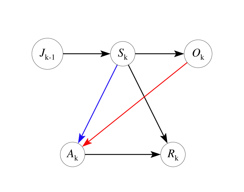
We have so far assumed that the evaluation policies are Markovian. In this section, we consider the case when evaluation policies are history-dependent, i.e., $\pi^{e}:\mathcal{O}\times\tilde{\mathcal{J}}_{t-1}\to\Delta(\mathcal{A})$ where $\tilde{\mathcal{J}}_{t-1}=\prod_{k=0}^{t-1}(\mathcal{O}\times\mathcal{A})$. Note $\tilde{\mathcal{J}}_{t-1}$ is different from $\mathcal{J}_{t-1}$ recalling $\mathcal{J}_{t-1}=\mathcal{O}\times\{\prod_{k=0}^{t-1}(\mathcal{O}\times\mathcal{A})\}$. We mainly analyze the value-function based estimator in this section.

We introduce the value and learnable bridge functions as follows. They are natural extensions of Assumption 3 and Definition 4 for history-dependent policies. Let $\mathfrak{\tilde{J}}_{j-1}=\{O_{0},A_{0},\cdots,O_{H-1},A_{H-1}\}$. Note this is contained in $\mathfrak{J}_{j-1}=\{O^{-}_{0},O_{0},A_{0},\cdots,O_{H-1},A_{H-1}\}$.

Assumption 6 (Existence of bridge functions).

There exist value bridge functions $\{b^{\prime[j]}_{V}\}_{j=0}^{H-1}$ defined as solutions to

$$\mathbb{E}[b^{\prime[j]}_{V}(A_{j},O_{j},\mathfrak{\tilde{J}}_{j-1})\mid A_{j},S_{j},\mathfrak{\tilde{J}}_{j-1}] =\mathbb{E}_{\pi^{e}}[\sum_{t=j}^{H-1}\gamma^{t-j}R_{t}\pi^{e}_{j}(A_{j}\mid{O_{j}},\mathfrak{\tilde{J}}_{j-1})|A_{j},S_{j},\mathfrak{\tilde{J}}_{j-1}].$$

There exist weight bridge functions $\{b^{\prime[j]}_{W}\}_{j=0}^{H-1}$ defined as solutions to

$$\mathbb{E}[b^{\prime[j]}_{W}(A_{j},\mathfrak{J}_{j-1})\mid A_{j},S_{j},\mathfrak{\tilde{J}}_{j-1}] =\mu_{j}(S_{j},\mathfrak{\tilde{J}}_{j-1})/\pi^{b}_{j}(A_{j}\mid S_{j})$$

where $\mu_{j}(S_{j},\mathfrak{\tilde{J}}_{j-1})$ is $P_{\pi^{e},j}(S_{j},\mathfrak{\tilde{J}}_{j-1})/P_{\pi^{b},j}(S_{j},\mathfrak{\tilde{J}}_{j-1})$.

Definition 5 (Learnable bridge functions).

Learnable value bridge functions $\{b^{[j]}_{V}\}_{j=0}^{H-1}$ are defined as solutions to

$$\begin{split}&\mathbb{E}[b^{[j]}_{V}(A_{j},O_{{j}},\mathfrak{\tilde{J}}_{j-1})\mid A_{j},\mathfrak{J}_{j-1}]=\mathbb{E}[R_{j}\pi^{e}_{j}(A_{j}\mid{O_{j}},\mathfrak{\tilde{J}}_{j-1})+\gamma\sum_{a^{\prime}}b^{[j+1]}_{V}(a^{\prime},{O_{j+1}},\mathfrak{\tilde{J}}_{j})\pi^{e}_{j}(A_{j}\mid{O_{j}},\mathfrak{\tilde{J}}_{j-1})\mid A_{j},\mathfrak{J}_{j-1}].\end{split}$$

It is worthwhile to note $\mathfrak{J}_{j}$ is contained in $\mathfrak{\tilde{J}}_{j}$. If evaluation policies depend on the whole $\mathfrak{J}_{j}$, it is unclear how to identify the policy value in our framework.

Now, we are ready to prove the identification formula.

Theorem 12.

• Suppose Assumption 6. Then, any learnable bridge function satisfies

  $$J(\pi^{e})=\mathbb{E}[\sum_{a}b^{[0]}_{V}(a,O_{0})].$$

• Suppose the existence of value bridge functions and the completness assumption:

  $$\mathbb{E}[g(S_{j},A_{j},\mathfrak{\tilde{J}}_{j-1})\mid A_{j},\mathfrak{J}_{j-1}]=0\implies g(\cdot)=0$$

  for any $0\leq j\leq H-1$. Then, any learnable bridge function satisfies

  $$J(\pi^{e})=\mathbb{E}[\sum_{a}b^{[0]}_{V}(a,O_{0})].$$

Similar to Section 5, $b_{V}$ can be estimated in a recursive fashion. In the tabular setting, the sufficient conditions to ensure the existence of value bridge functions and the completness is

$${\rm rank}(\mathrm{Pr}(\mathbf{O}_{j}\mid A_{j}=a,\mathbfcal{J}_{j-1}))=|{\mathcal{S}}|.$$

The nonasymptotic properties of the resulting estimator can be similarly established as in Section 4.3

7 Experiments

In this section, we evaluate the empirical performance of our method using two synthetic datasets. In both datasets, the state spaces are continuous. Hence, existing POMDP evaluation methods such as Tennenholtz et al. (2020) and Nair and Jiang (2021) are not directly applicable. The discounted factor $\gamma$ is fixed to 0.95 in all experiments.

7.1 One-Dimensional Dynamic Process

Environment  We first consider a simple dynamic process with a one-dimensional continuous state space and binary actions. Similar environments have been considered in the literature (see e.g., Shi et al., 2022). The initial state distribution, reward function and state transition are given by

$$S_{0}\sim\mathcal{N}(0,0.5^{2}),\quad R_{t}=S_{t}+2A_{t-1}-1,$$

$$S_{t+1}=0.5S_{t}+(2A_{t}-1)+\mathcal{N}(0,0.5^{2}),$$

respectively. The observation is generated according to the additive noise model, $O_{t}=S_{t}+N(0,\sigma_{O}^{2})$. Here, the variance parameter $\sigma_{O}$ characterizes the degree of partial observability and hence the degree of unmeasured confounding. In the extreme case where $\sigma_{O}=0$, the states become fully-observable and no unmeasured confounders exist. We set the behavior and target policies to be sigmoid functions of the state and the observation, respectively,

$$\pi^{b}(1|s)=\frac{1}{1+\exp(s+1)},\pi^{e}_{w}(1|o)=\frac{1}{1+\exp(wo+1)},$$

for $w\in\{-3,-2,1,2\}$.

Figure 4: Logarithms of relative biases and mean squared errors (see Appendix D for the detailed definitions) of the proposed and the baseline methods, with difference choices of $w$ and sample sizes. Confidence intervals are calculated from 10 simulations. Upper panels: sample size equals 2e5. $\sigma_{O}$ equals $0.5$, $1.0$ and $1.5$, from left to right. Bottom panels: $\sigma_{O}$ is fixed to 1.

Figure 5: Logarithms of relative biases (left) and MSEs (right) of the proposed (solid lines) and the baseline (dashed lines) estimators and the associated confidence interval, based on 10 simulations, with different choices of the temperature parameter $\tau_{O}$. Observation in top panels is generated by injecting Gaussian noises whereas the location of the cart is removed from the observation in bottom panels.

Implementation and Baseline Method  We use linear basis functions to approximate the bridge functions. In this case, the proposed three estimators ($\hat{J}_{\mathrm{VM}},\hat{J}_{\mathrm{IS}},\hat{J}_{\mathrm{DR}}$) coincide with each other (see a similar phenomenon in Uehara et al., 2020), so we compute the value function-based estimator only. We compare our estimator to the standard linear value function-based estimator that assumes no unmeasured confounders, i.e., LSTDQ (Lagoudakis and Parr, 2003). See additional implementation details in Appendix D.

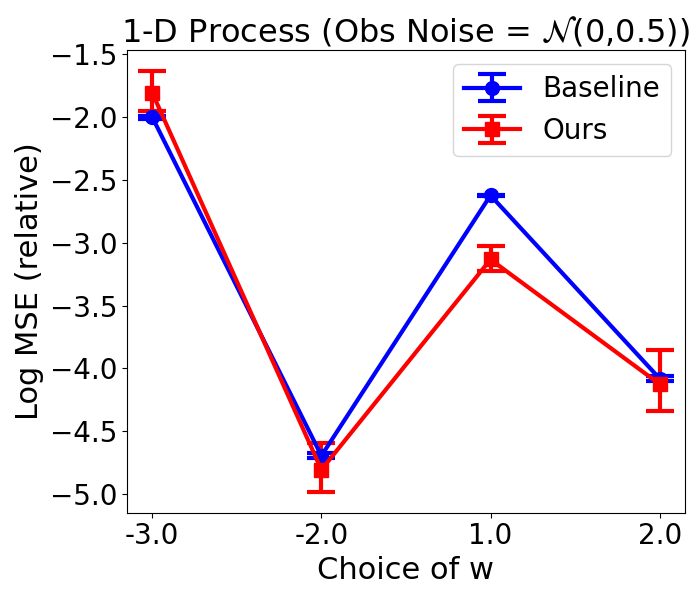
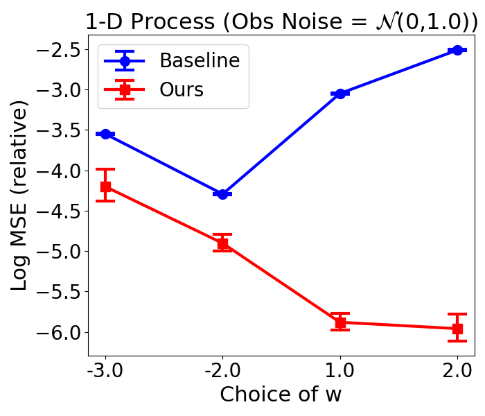
Results  For each simulation, we first generate 2000 trajectories with 100 time points per trajectory. This yields a total of 2e5 observations. Reported in the upper panels of Figure 4 are the logarithms of relative mean squared errors of the proposed and baseline methods, with different choices of $\omega$ and $\sigma_{O}$. We make a few observations. First, when $\sigma_{O}\geq 1$, the proposed estimator is significantly better than the baseline estimator. Second, when $\sigma_{O}=0.5$, the two methods perform comparably. As we have commented, $\sigma_{O}$ measures the degree of unmeasured confounding. For moderately large $\sigma_{O}$, the baseline estimator cannot handle unmeasured confounders, yielding a biased estimator. In contrast, a smaller $\sigma_{O}$ produces a less confounded dataset. The two estimators thus achieve similar performance.

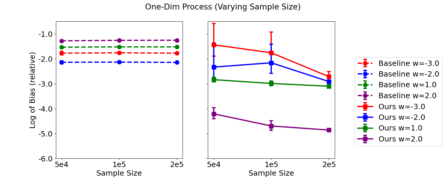
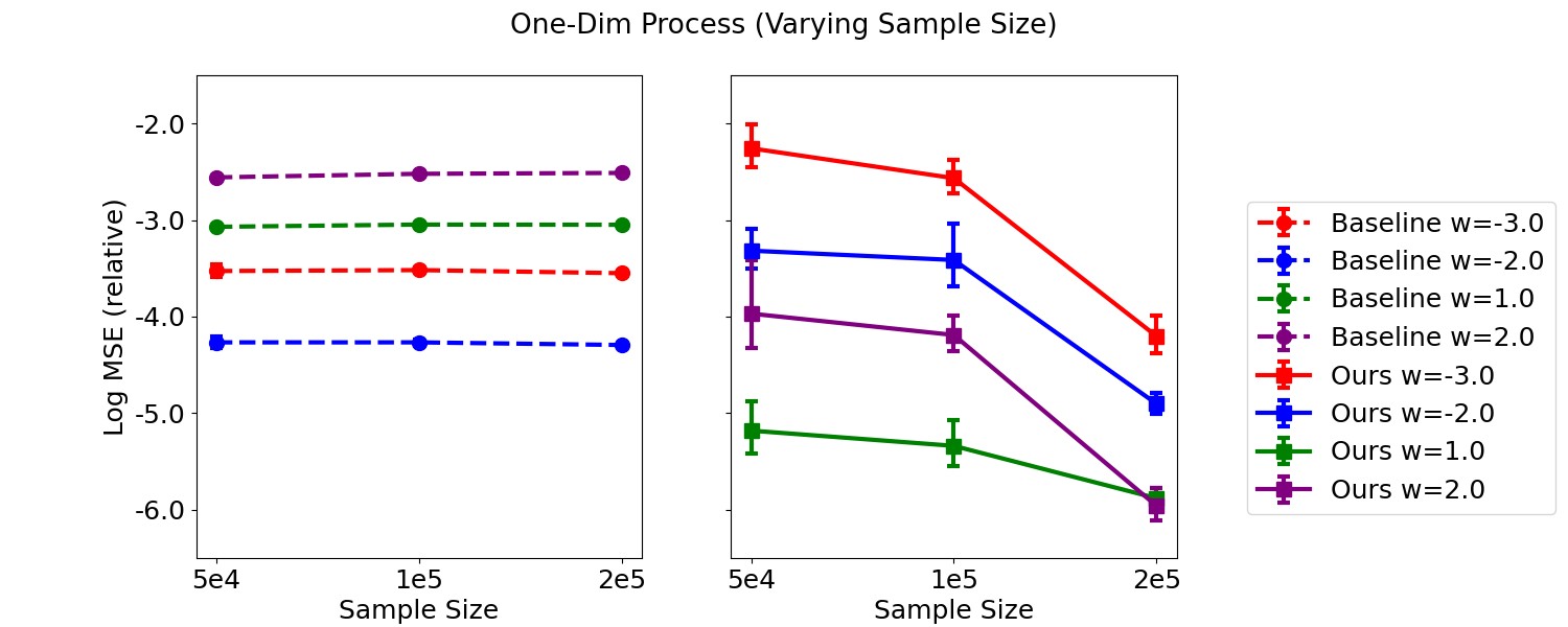
We next fix $\sigma_{O}$ to 1.0, vary the number of trajectories generated in each simulation, and report the corresponding relative biases and mean squared errors of the proposed and baseline methods as well as the associated confidence intervals in the bottom panels of Figure 4 and Figure 6 (see Appendix D). It can be seen that the baseline estimator suffers from a large bias. Their bias and MSE are constant as functions of sample size. To the contrary, the bias and MSE of the proposed estimator generally decrease with the sample size, demonstrating its consistency.

7.2 CartPole

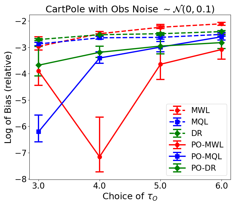
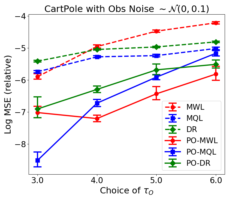
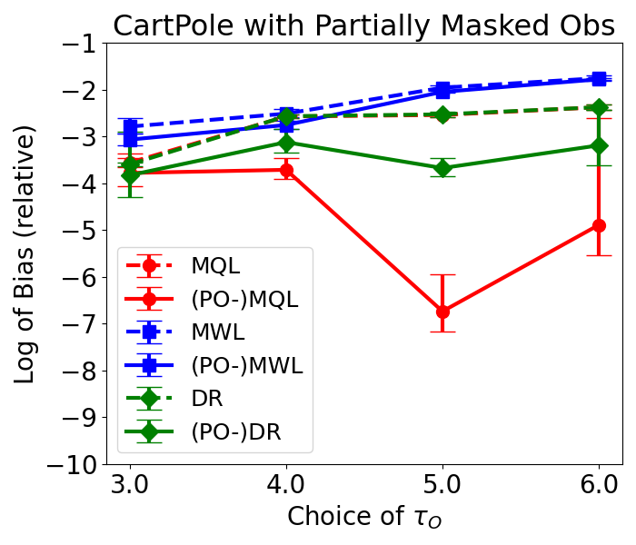
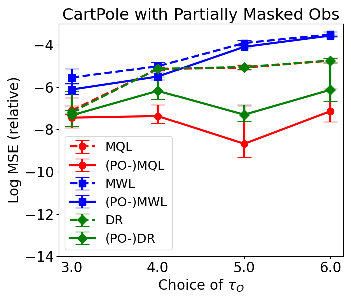
We next consider the CartPole environment from the OpenAI Gym environment (Brockman et al., 2016). The state variables are 4-dimensional and fully-observable. To create partially observable environments, we simulate observations by either adding independent Gaussian noises to each dimension of the states, i.e., $O^{(j)}=S^{(j)}(1+\mathcal{N}(0,0.1^{2}))$, $1\leq j\leq 4$, or removing the location of the cart from the observation. To generate data, we apply DQN (Mnih et al., 2015) to the data that include latent states instead of observations, and set the behavior policy to a softmax policy based on the estimated Q-function. The evaluation policy is set to another softmax policy based on DQN applied to the observational data (i.e., no latent states) with the temperature parameter given by $\tau_{O}$. For each simulation, we collect the dataset according to the behavior policy until the sample size reaches 2e5. We consider three baseline estimators, corresponding to the minimax Q-learning (MQL), minimax weight learning (MWL) and DR estimators (Uehara et al., 2020). These estimators cannot handle unmeasured confounders. The proposed value function-based, marginalized IS and DR estimators are denoted by PO-MQL, PO-MWL and PO-DR, respectively. We parametrize the bridge functions using a two-layer neural network, and set the function spaces $\mathcal{V}^{\dagger}$ and $\mathcal{W}^{\dagger}$ to RKHSs to facilitate the computation. Some additional details about the environment and implementation are given in Appendix D. Results are reported in Figures 5. It can be seen that the proposed estimator achieves better performance in all cases.

8 Conclusion

We study OPE on POMDPs where behavior policies depend on unobserved state variables. We propose a novel identification method for the target policy’s value in the presence of unmeasured confounders. Our proposal only relies on the existence of bridge functions. We further propose minimax learning methods for computing these estimated bridge functions that can be naturally coupled with function approximation to handle a continuous or large state/observation space. We also develop three types of policy value estimators based on the bridge function estimators and provide their nonasymptotic and asymptotic properties. In Section A, we discuss the different between our proposal and a highly-related concurrent work by Bennett and Kallus (2021).

Appendix A Additional Related Works

We discuss some additional related works in this section.

Minimax Estimation

Our proposal defines the value and weight bridge functions as solutions to some integral equations. Nonparametrically estimating these bridge functions is closely related to nonparametric instrumental variables (NPIV) estimation. In NPIV estimation, the standard regression estimator is biased and variants of minimax estimation methods have been developed to correct the bias (Dikkala et al., 2020; Muandet et al., 2019; Hartford et al., 2017; Bennett and Kallus, 2020). In the RL literature, the minimax learning method has also been widely used for OPE without unmeasured confounders Antos et al. (2008); Chen and Jiang (2019); Nachum et al. (2019); Feng et al. (2019); Uehara et al. (2020).

Negative Controls

Our proposal is closely related to a line of research on developing causal inference methods to evaluate the average treatment effect (ATE) with double-negative control adjustment. Among those works, Miao et al. (2018) outlined a consistent estimator for ATE with a categorical confounder. More recent methods generalize their approach to the continuous confounder setting Deaner (2018); Cui et al. (2020); Singh (2020); Ghassami et al. (2021); Xu et al. (2021); Mastouri et al. (2021). All the aforementioned methods focus on a contextual bandit setting (i.e., one-shot decision making) and are not directly applicable to POMDPs that involve sequential decision making.

Comparison with Bennett and Kallus (2021)

The difference between the work of Bennett and Kallus (2021) and our proposal can be summarized as follows. Methodologically, the IS, VM, DR estimators developed in the two papers are different. First, consider the IS estimator as an example. In fully-observable MDPs, our proposed estimator is reduced to marginal IS estimators (Liu et al., 2018; Xie et al., 2019) whereas the IS estimator developed by Bennett and Kallus (2021) is reduced to the cumulative IS estimator (Precup, 2000). Second, Bennett and Kallus (2021) do not introduce value bridge functions as in our paper. Instead, they introduce an outcome bridge function to approximate the reward function at each time step $0\leq t\leq H-1$. Because of the difference between these definitions, their estimating procedure for the outcome bridge functions involves the estimated weight bridge functions. In contrast, the estimation of value bridge functions in our paper is agnostic to the estimation of weight bridge function.

Theoretically, we focus on the derivation of finite-sample error bounds. To the contrary, Bennett and Kallus (2021) focus on establishing asymptotic properties. In addition, the efficiency bound they developed differs from ours (see Theorem 7). Specifically, they focused on the non-tabular case whereas our bounded is limited to the tabular setting. Moreover, since we focus on evaluating Markovian and stationary policies, in fully-observable MDPs, our bounds are reduced to those in Kallus and Uehara (2019) whereas their bound is reduced to the one in Jiang and Li (2016).

Appendix B Some Additional Details Regarding OPE in Partially Observable Contextual Bandits

We specialize our results in Section 3 to tabular settings. We use the following notation. Let $X,Y$ be random variables taking values $\{x_{1},\cdots,x_{n}\}$ and $\{y_{1},\cdots,y_{m}\}$, respectively. Then we denote a $n\times m$ matrix with elements $\mathrm{Pr}(x_{i}\mid y_{j})$ by $\mathrm{Pr}(\mathbf{X}\mid\mathbf{Y})$. Similarly, $\mathrm{Pr}(\mathbf{X})$ denotes a $n$-dimensional vector with elements $x_{i}$. We denote the Moore-penrose inverse of $\mathrm{Pr}(\mathbf{X}\mid\mathbf{Y})$ by $\mathrm{Pr}(\mathbf{X}\mid\mathbf{Y})^{+}$.

We next introduce the following assumption.

Assumption 7.

Suppose ${\rm rank}(\mathrm{Pr}_{\pi^{b}}(\mathbf{O}_{0}|\mathbf{S}_{0}))=|{\mathcal{S}}|$ and ${\rm rank}(\mathrm{Pr}_{\pi^{b}}(\mathbf{O}_{-1}|\mathbf{S}_{0}))=|{\mathcal{S}}|$.

As we have mentioned, Assumption 7 implies that $|\mathcal{O}|\geq|\mathcal{S}|$ and is weaker than the condition in Tennenholtz et al. (2020) that requires the state and observation spaces have the same cardinality. The following lemma states that 7 is equivalent to Assumption 2 in Nair and Jiang (2021).

Lemma 5.

Suppose overlap conditions:

$$\mathrm{Pr}_{\pi^{b}}(O^{-}=o^{-}\mid A_{0}=a)>0,\quad\mathrm{Pr}_{\pi^{b}}(O^{-}=o^{-}\mid A_{0}=a)>0$$

for any $(s,a,o)\in{\mathcal{S}}\times\mathcal{A}\times\mathcal{O}$. Then, Assumption 7 holds if and only if ${\rm rank}(\mathrm{Pr}_{\pi^{b}}(\mathbf{O}_{0}|A_{0}=a,\mathbf{O}_{-1}))=|{\mathcal{S}}|$ for any $a\in\mathcal{A}$.

Then following Nair and Jiang (2021), the policy value can be explicitly identified as follows:

Theorem 13 (Identification formula in the tabular setting).

$$J(\pi^{e})=\sum_{a,r,o}r\pi^{e}_{0}(a|o)\mathrm{Pr}_{\pi^{b}}(r,o|\mathbf{O}_{-1})\{\mathrm{Pr}_{\pi^{b}}(\mathbf{O}_{0}|A_{0}=a,\mathbf{O}_{-1})\}^{+}\mathrm{Pr}_{\pi^{b}}(\mathbf{O}_{0}).$$

Appendix C Some Additional Details Regarding OPE in Time-Homogeneous POMDPs

As we have commented, we can use linear basis functions or RKHSs to estimate the bridge functions. Specifically, when $\mathcal{V}^{\dagger}$ or $\mathcal{W}^{\dagger}$ is set to be the unit ball in an RKHS, then there exists a close form expression for the inner maximization problem (see e.g., Liu et al., 2018). When linear basis functions are used, the proposed minimax optimization has explicit solutions, as we elaborate in the example below.

Example 1 (Linear models).

Let $\mathcal{V}=\mathcal{V}^{\dagger}=\{(a,o)\mapsto\theta^{\top}\phi(a,o):\theta\in\Theta\}$ and $\lambda=0$, where $\phi:\mathcal{A}\times\mathcal{O}\to\mathbb{R}^{d}$ is a feature vector and $\Theta\subset\mathbb{R}^{d}$. When the parameter space $\Theta$ is sufficiently large, it is immediate to see that

$$\hat{b}_{V}=\left(\mathbb{E}_{\mathcal{D}}[\phi(A,O^{-})\phi^{\top}(A,O)]-\gamma\mathbb{E}_{\mathcal{D}}\left[\sum_{a^{\prime}}\pi^{e}(A\mid O)\phi(A,O^{-})\phi^{\top}(a^{\prime},O^{+})\right]\right)^{+}\mathbb{E}_{\mathcal{D}}[R\pi^{e}(A\mid O)\phi(A,O^{-})].$$

The resulting policy value estimator is given by

$$\mathbb{E}_{\mathcal{D}}[\sum_{a}\phi(a,O)]^{\top}\left(\mathbb{E}_{\mathcal{D}}[\phi(A,O^{-})\phi^{\top}(A,O)]-\gamma\mathbb{E}_{\mathcal{D}}\left[\sum_{a^{\prime}}\pi^{e}(A\mid O)\phi(A,O^{-})\phi^{\top}(a^{\prime},O^{+})\right]\right)^{+}\mathbb{E}_{\mathcal{D}}[R\pi^{e}(A\mid O)\phi(A,O^{-})].$$

Consider the standard MDP setting where $S=O=O^{-},S^{+}=O^{+}$. By setting $\mathcal{V}=\{(s,a)\mapsto\theta^{\top}\pi^{e}(a\mid s)\phi(a,s)\},\mathcal{V}^{\dagger}=\{(s,a)\mapsto\theta^{\top}\phi(a,s)/\pi^{e}(a\mid s)\}$, the above estimator reduces to classical LSTDQ estimator Lagoudakis and Parr (2003):

$$\mathbb{E}_{\mathcal{D}}[\phi(\pi^{e},S)]^{\top}\left(\mathbb{E}_{\mathcal{D}}[\phi(A,S)\phi^{\top}(A,S)]-\gamma\mathbb{E}_{\mathcal{D}}\left[\phi(A,S)\phi^{\top}(\pi^{e},S^{+})\right]\right)^{+}\mathbb{E}_{\mathcal{D}}[R\phi(A,S)],$$

where $\phi(\pi^{e},s)=\mathbb{E}_{a\sim\pi^{e}(s)}[\phi(a,s)]$.

Alternatively, we may set $\mathcal{V}:=\{(a,o)\rightarrow\pi^{e}(a|o)\theta^{\top}\phi(a,o):\theta\in\Theta\}$ instead. As discussed in Section 7.1, we find such a parametrization has smaller approximation error in the implementation. The corresponding estimator is given by

$$\mathbb{E}_{O\sim\nu_{O},a\sim\pi^{e}(\cdot|O)}[\phi(a,O)]^{\top}\big{(}\mathbb{E}_{\mathcal{D}}[ \phi(A,O^{-})\phi^{\top}(A,O)\pi^{e}(A\mid O)$$

$$-\gamma{\phi(A,O^{-})\pi^{e}(A\mid O)\mathbb{E}_{a^{\prime}\sim\pi^{e}(\cdot|O^{+})}[\phi^{\top}(a^{\prime},O^{+})]}]\big{)}^{+}\mathbb{E}_{\mathcal{D}}[R\pi^{e}(A\mid O)\phi(A,O^{-})].$$

We next introduce two examples to further elaborate Theorem 4.

Example 2 (Tabular models).

Consider the tabular case, and $\mathcal{V}$ and $\mathcal{V}^{\dagger}$ are fully expressive classes, i.e., linear in the one-hot encoding vector over $(\mathcal{A}\times\mathcal{O})$. Then, $\log(|\mathcal{V}||\mathcal{V}^{\dagger}|)$ is substituted by $|\mathcal{O}||\mathcal{A}|$. The Bellman closedness ${\mathcal{T}}\mathcal{V}\subset\mathcal{V}^{\dagger}$ is satisfied. Our finite sample result circumvents the potentially complicated matrix concentration argument in POMDPs (see e.g., Hsu et al., 2012) by viewing the problem from a general perspective.

Example 3 (Linear models).

Consider the case where $\mathcal{V}$ and $\mathcal{V}^{\dagger}$ are linear models. Then, $\log(|\mathcal{V}||\mathcal{V}|^{\dagger})$ can be substituted by the dimension of the feature vector $d$. The Bellman closedness assumption is satisfied when $P_{\pi^{b}}(R,O,O^{+}\mid A,O^{-})$ is linear in $\phi(A,O^{-})$. In fully-observable MDPs, this reduces to the linear MDP model (Jin et al., 2020), i.e., $P_{\pi^{b}}(R,S^{+}\mid A,S)$ is linear in $\phi(A,S)$.

The next theorem shows that the finite sample rate of convergence for the value function-based estimator can be established without any closedness assumption.

Theorem 14 (Convergence rate without closedness).

Set $\lambda$ in equations 8 and 9 to zero. Suppose (a) Assumption 2 holds so that the bridge functions exist; (b) $\mathcal{V}$ and $\mathcal{V}^{\dagger}$ are symmetric finite hypothesis classes; (c) $\mathcal{V}$ contains certain learnable reward bridge function; (d) $\mathcal{V}^{\dagger}$ contains learnable weight bridge function; (e) $\forall v\in\mathcal{V},\|v\|_{\infty}\leq C_{\mathcal{V}}$ and $\forall v\in\mathcal{V}^{\dagger},\|v\|_{\infty}\leq C_{\mathcal{V}^{\dagger}}$. Then, with probability $1-\delta$,

$$|J(\pi^{e})-\hat{J}_{\mathrm{VM}}|\leq c\max(1,C_{\mathcal{V}},C_{\mathcal{V}^{\dagger}})^{2}(1-\gamma)^{-2}\sqrt{\log(|\mathcal{V}||\mathcal{V}^{\dagger}|c/\delta)/n},$$

for some universal constant $c>0$.

Next, we discuss the theoretical properties of the IS estimator. To establish its convergence rate, we can define the adjoint Bellman residual operator ${\mathcal{T}}^{\prime}$ as in Uehara et al. (2021), and derive the convergence rate of $\mathbb{E}[\{{\mathcal{T}}^{\prime}\hat{b}_{W}(A,O^{+})\}^{2}]^{1/2}$ under realizability ($b_{W}\in\mathcal{W}$) and (adjoint) closedness (${\mathcal{T}}^{\prime}\mathcal{W}\subset\mathcal{W}^{\dagger}$). Similar to the proof of Theorem 5, this (adjoint) Bellman residual error can be translated into the error of the estimated policy value. Without the closedness assumption, similar results can be derived when $b_{W}\in\mathcal{W}$ and $b_{V}\in\mathcal{W}^{\dagger}$.

Appendix D Experiments

Measure of Estimation Error

Given $n$ datasets $D_{1},D_{2},...,D_{n}$, the estimators computed based on each dataset $\hat{V}_{1},...,\hat{V}_{n}$, and the true value $V$, we define the relative bias to be

$$|\frac{1}{n}\sum_{i=1}^{n}\frac{\hat{V}_{i}}{V}-1|.$$

Define the relative mean squared error to be:

$$|\frac{1}{n}\sum_{i=1}^{n}\Big{(}\frac{\hat{V}_{i}-V}{V}\Big{)}^{2}|.$$

In our experiments, we use the above two definitions to measure the estimation error of different estimators.

Additional Details for the 1d Continuous Dynamic Process Example

Notice that the definition of the bridge value function involves the evaluation policy. Instead of directly using linear models to parametrize $b_{V}$, we set the function space to $\mathcal{V}:=\{(a,o)\rightarrow\pi^{e}(a|o)\theta^{\top}\phi(a,o):\theta\in\Theta\}$. We find that such a parametrization has smaller approximation error. The closed-form expression of the resulting estimator is given in Section C. We use the Python function RBFsampler to generate random Fourier features. To mitigate the randomness arising from the features, for each dataset and each method, we use 5 different random seeds to generate 5 sets of RBF features and use the average value as the final estimator. The RBF kernel is set to $\exp(-5x^{2})$, and the feature dimension is set to 100.

Additional Figures

We next report the relative MSE of the two estimators in the following figure.

Figure 6: Experiments with varying sample size. Noise Level $\sigma_{O}=1.0$

CartPole Environment

The state space is 4-dimensional, including position and velocity of cart, and angle and angle velocity of pole. The action space is $\{0,1\}$, corresponding to pushing the cart to the left or to the right. In addition, we use a modified reward function to better distinguish values among different policies. Specifically, the reward is defined as

$$r=|2.0-\frac{x}{x_{\text{clip}}}|\cdot|2.0-\frac{\theta}{\theta_{\text{clip}}}|-1.0$$

where $x$ and $\theta$ are the position of Cart and angle of Pole, respectively, and $x_{\text{clip}}$ and $\theta_{\text{clip}}$ are the thresholds such that the episode will terminate (done = True) when either $|x|\geq x_{clip}$ or $|\theta|\geq\theta_{clip}$. Under this definition, the reward will be larger when the cart is closer to the center and the angle of the pole is closer to perpendicular. It is straightforward to show that $r$ is bounded between 0 and 3. Since we set $\gamma=0.5$, the value is bounded between 0 and 60.

CartPole Implementation

We set the adversarial function spaces $\mathcal{V}^{\dagger}$ and $\mathcal{W}^{\dagger}$ to RKHSs to facilitate the computation. Both $b_{v}$ in PO-MQL and $b_{w}$ in PO-MWL are parameterized by a two-layer neural network with layer width = 256 and ReLU as activation function, and are optimized by a kernel loss function (see the derivation below).

In the following, we use $K(x_{1};x_{2})$ to denote the RBF kernel:

$$K(x_{1};x_{2}):=\exp(-\frac{\|x_{1}-x_{2}\|_{2}}{2\beta^{2}})$$

where $\beta$ denotes the bandwidth parameter. We choose $\beta=\text{med}/2$ during the training of PO-MWL ($b_{w}$) or MWL, and $\beta=\text{med}/5$ for PO-MQL ($b_{v}$) or MQL, where “med” is the median of the l2-distance over the samples in the dataset.

Derivation of the Loss Function for PO-MQL ($b_{v}$)

Similar to the experiments in Toy environments, we reparameterize $g$ function with $\bar{g}\cdot\pi^{e}$, and therefore the predictor with $g$ should be adjusted by replacing $g$ with $\bar{g}\cdot\pi^{e}$:

$$\mathbb{E}_{O\sim\nu_{O},A\sim\pi^{e}}[\bar{g}(O,A)\pi^{e}(A|O)].$$

The loss function is given by:

$$\max_{f}L_{V}^{2}(g,f)= \max_{f}\Big{(}\mathbb{E}[(R\pi^{e}(A|O)+\gamma\mathbb{E}_{a^{\prime}\sim\pi^{e}}[g(a^{\prime},O^{+})]\pi^{e}(A|O)-g(A,O)\pi^{e}(A|O))f(A,O^{-})]\Big{)}^{2}$$

$$= \max_{f}\Big{(}\Big{\langle}f,\mathbb{E}[R\pi^{e}(A|O)+\gamma\mathbb{E}_{a^{\prime}\sim\pi^{e}}[g(a^{\prime},O^{+})]\pi^{e}(A|O)-g(A,O)\pi^{e}(A|O)]K(A,O^{-};\cdot)\Big{\rangle}_{\mathcal{H}_{K}}\Big{)}^{2}$$

$$= \mathbb{E}[\Big{(}R\pi^{e}(A|O)+\gamma\mathbb{E}_{a^{\prime}\sim\pi^{e}}[g(a^{\prime},O^{+})]\pi^{e}(A|O)-\pi^{e}(A|O)g(A,O)\Big{)}K(A,O^{-};\bar{A},\bar{O}^{-})$$

$$\cdot\Big{(}\bar{R}\pi^{e}(\bar{A}|\bar{O})+\gamma\mathbb{E}_{\bar{a}^{\prime}\sim\pi^{e}}[g(\bar{a}^{\prime},\bar{O}^{+})]\pi^{e}(\bar{A}|\bar{O})-\pi^{e}(\bar{A}|\bar{O})g(\bar{A},\bar{O})\Big{)}].$$

Derivation of the Loss Function for PO-MWL ($b_{w}$)

Similarly, we reparameterize $f$ function with $\bar{f}\cdot\pi^{e}$. Since we do not change the parameterization of $b_{w}$, we only need to adjust the loss function without changing the estimator:

$$\max_{f}L^{2}_{W}(g,f)$$

$$= \max_{f}\Big{(}\mathbb{E}[\gamma g(O^{-},A)\pi^{e}(A|O)\sum_{a^{\prime}}f(O^{+},a^{\prime})-g(O^{-},A)f(O,A)]+(1-\gamma)\mathbb{E}_{O\sim\nu_{O}}[\sum_{a^{\prime}}f(O,a^{\prime})]\Big{)}^{2}$$

$$= \max_{f}\Big{(}\mathbb{E}[\gamma g(O^{-},A)\pi^{e}(A|O)\mathbb{E}_{a^{\prime}\sim\pi^{e}(\cdot|O^{+})}[\bar{f}(O^{+},a^{\prime})]-g(O^{-},A)\pi^{e}(A|O)\bar{f}(O,A)]+(1-\gamma)\mathbb{E}_{O\sim\nu_{O},a^{\prime}\sim\pi^{e}}[\bar{f}(O,a^{\prime})]\Big{)}^{2}$$

$$= \max_{f}\Big{(}\mathbb{E}[\gamma g(O^{-},A)\pi^{e}(A|O)\mathbb{E}_{a^{\prime}\sim\pi^{e}(\cdot|O^{+})}[\langle\bar{f},K(O^{+},a^{\prime};\cdot){\textnormal{a}}]-g(O^{-},A)\pi^{e}(A|O)\langle\bar{f},K(O,A;\cdot){\textnormal{a}}]$$

$$+(1-\gamma)\mathbb{E}_{O\sim\nu_{O},a^{\prime}\sim\pi^{e}}[\langle\bar{f},K(O,a^{\prime};\cdot){\textnormal{a}}]\Big{)}^{2}$$

$$= \max_{f}\Big{(}\langle\bar{f},\mathbb{E}[\gamma g(O^{-},A)\pi^{e}(A|O)\Big{(}\mathbb{E}_{a^{\prime}\sim\pi^{e}(\cdot|O^{+})}[K(O^{+},a^{\prime};\cdot)]-K(O,A;\cdot)\Big{)}]+(1-\gamma)\mathbb{E}_{O\sim\nu_{O},a^{\prime}\sim\pi^{e}}[K(O,a^{\prime};\cdot)]{\textnormal{a}}\Big{)}^{2}$$

$$= \mathbb{E}[g(O^{-},A)\pi^{e}(A|O)g(\bar{O}^{-},\bar{A})\pi^{e}(\bar{A}|\bar{O})\cdot$$

$$\quad\quad\quad\Big{(}\gamma^{2}K(O^{+},\pi^{e};\bar{O}^{+},\pi^{e})+K(O,A;\bar{O},\bar{A})-\gamma K(O^{+},\pi^{e};\bar{O},\bar{A})-\gamma K(O,A;\bar{O}^{+},\pi^{e})\Big{)}]$$

$$+(1-\gamma)^{2}\mathbb{E}[K(O_{0},\pi^{e};\bar{O}_{0},\pi^{e})]$$ (no gradient)

$$+\gamma(1-\gamma)\mathbb{E}[g(O^{-},A)\pi^{e}(A|O)K(O^{+},\pi^{e};\bar{O}_{0},\pi^{e})+g(\bar{O}^{-},\bar{A})\pi^{e}(\bar{A}|\bar{O})K(O_{0},\pi^{e};\bar{O}^{+},\pi^{e})]$$

$$-(1-\gamma)\mathbb{E}[g(O^{-},A)\pi^{e}(A|O)K(O,A;\bar{O}_{0},\pi^{e})+g(\bar{O}^{-},\bar{A})\pi^{e}(\bar{A}|\bar{O})K(O_{0},\pi^{e};\bar{O},\bar{A})].$$

where we denote

$$K(O,\pi^{e};\bar{O},\pi^{e}):=\mathbb{E}_{a^{\prime}\sim\pi^{e}(\cdot|O),\bar{a}^{\prime}\sim\pi^{e}(\cdot|\bar{O})}[K(O,a^{\prime};\bar{O},\bar{A}),\quad K(O,\pi^{e};\bar{O},\bar{A}):=\mathbb{E}_{a^{\prime}\sim\pi^{e}(\cdot|O)}[K(O,a^{\prime};\bar{O},\bar{A})].$$

Loss Function for Baseline Estimators

We follow Uehara et al. (2020) to define the MQL and MWL loss function with the adversarial function space given by RHKSs. The loss function for MQL is given by:

$$\max_{f}L_{q}^{2}(f,q)= \mathbb{E}[\Big{(}R+\gamma\mathbb{E}_{a^{\prime}\sim\pi^{e}(\cdot|O^{+})}[q(a^{\prime},O^{+})]-q(A,O)\Big{)}K(A,O;\bar{A},\bar{O})\Big{(}\bar{R}+\gamma\mathbb{E}_{\bar{a}^{\prime}\sim\pi^{e}(\cdot|\bar{O}^{+})}[q(\bar{a}^{\prime},\bar{O}^{+})]-q(\bar{A},\bar{O})\Big{)}].$$

The loss function for MWL is given by:

$$\max_{f}L_{w}^{2}(f,w)$$

$$= \mathbb{E}[w(O,A)w(\bar{O},\bar{A})\Big{(}K(O^{+},\pi^{e};\bar{O}^{+},\pi^{e})+K(O,A;\bar{O},\bar{A})-\gamma K(O^{+},\pi^{e};\bar{O},\bar{A})-\gamma K(O,A;\bar{O}^{+},\pi^{e})\Big{)}]$$

$$+(1-\gamma)^{2}\mathbb{E}[K(O_{0},\pi^{e};\bar{O}_{0},\pi^{e})]$$ (no gradient)

$$+\gamma(1-\gamma)\mathbb{E}[w(O,A)K(O^{+},\pi^{e};\bar{O}_{0},\pi^{e})+w(\bar{O},\bar{A})K(O_{0},\pi^{e};\bar{O}^{+},\pi^{e})]$$

$$-(1-\gamma)\mathbb{E}[w(O,A)K(O,A;\bar{O}_{0},\pi^{e})+w(\bar{O},\bar{A})K(O_{0},\pi^{e};\bar{O},\bar{A})].$$

In addition, we use the same neural network architecture and the same choice of bandwidth during the training of MQL/MWL as those for PO-MQL/PO-MWL.

Appendix E Omitted proof

E.1 Proof of Section 3

Proof of Lemma 1.

First, we prove the value-function based identification formula:

$$\mathbb{E}[\sum_{a}b^{\prime}_{V}(a,O_{0})]=\mathbb{E}[\sum_{a}\mathbb{E}[b^{\prime}_{V}(a,O_{0})|S_{0}]]=\mathbb{E}[\sum_{a}\mathbb{E}[b^{\prime}_{V}(a,O_{0})|A_{0}=a,S_{0}]] A_{0}\perp O_{0}\mid S_{0}$$ ()

$$=\mathbb{E}[\sum_{a}\mathbb{E}[R_{0}\pi^{e}(a|O_{0})|A_{0}=a,S_{0}]]$$ (Definition of bridge functions)

$$=\mathbb{E}[\sum_{a}\mathbb{E}[R_{0}|A_{0}=a,S_{0}]\mathbb{E}[\pi^{e}(a\mid O_{0})\mid A_{0}=a,S_{0}]] R_{0}\perp O_{0}\mid A_{0},S_{0}$$ ( )

$$=\mathbb{E}[\sum_{a}\mathbb{E}[R_{0}|A_{0}=a,S_{0}]\mathbb{E}[\pi^{e}(a\mid O_{0})\mid S_{0}]] A_{0}\perp O_{0}\mid S_{0}$$ ()

$$=\mathbb{E}[\sum_{a}\mathbb{E}[R_{0}|A_{0}=a,S_{0}]\pi^{e}(a\mid O_{0})]$$

$$=J(\pi^{e}).$$ (From standard regression formula)

Second, we prove the importance sampling identification formula:

$$\mathbb{E}[b_{W}(A_{0},O^{-}_{0})R_{0}\pi^{e}(A_{0}\mid O_{0})]=\mathbb{E}[\mathbb{E}[b^{\prime}_{W}(A_{0},O^{-}_{0})\mid S_{0},A_{0}]R_{0}\pi^{e}(A_{0}\mid O_{0})] O^{-}_{0}\perp R_{0}\mid S_{0},A_{0}$$ ()

$$=\mathbb{E}[1/\pi^{b}(A_{0}\mid S_{0})\pi^{e}(A_{0}\mid O_{0})R_{0}] b^{\prime}_{W}$$ (Definition of )

$$=J(\pi^{e}).$$ (From standard IPW formula)

∎

Proof of Lemma 2.

We first prove reward bridge functions are learnable reward bridge functions:

$$\mathbb{E}[R_{0}\pi^{e}(A_{0}|O_{0})\mid A_{0},O^{-}_{0}]=\mathbb{E}[\mathbb{E}[R_{0}\pi^{e}(A_{0}|O_{0})\mid A_{0},S_{0},O^{-}_{0}]\mid A_{0},O^{-}_{0}]$$

$$=\mathbb{E}[\mathbb{E}[R_{0}\pi^{e}(A_{0}|O_{0})\mid A_{0},S_{0}]\mid A_{0},O^{-}_{0}] R_{0},O_{0}\perp O^{-}_{0}\mid S_{0},A_{0}$$ ( )

$$=\mathbb{E}[\mathbb{E}[b^{\prime}_{V}(A_{0},O_{0})\mid A_{0},S_{0}]\mid O^{-}_{0},A_{0}]$$ (Definition of bridge functions)

$$=\mathbb{E}[\mathbb{E}[b^{\prime}_{V}(A_{0},O_{0})\mid S_{0},O^{-}_{0},A_{0}]\mid O^{-}_{0},A_{0}] O_{0}\perp O^{-}_{0}\mid S_{0},A_{0}$$ ( )

$$=\mathbb{E}[b^{\prime}_{V}(A_{0},O_{0})\mid O^{-}_{0},A_{0}].$$

Next, we prove weight bridge functions are learnable weight bridge functions:

$$\mathbb{E}[b^{\prime}_{W}(A_{0},O^{-}_{0})\mid A_{0},O_{0}]=\mathbb{E}[\mathbb{E}[b^{\prime}_{W}(A_{0},O^{-}_{0})\mid A_{0},O_{0},S_{0}]\mid A_{0},O_{0}]$$

$$=\mathbb{E}[\mathbb{E}[b^{\prime}_{W}(A_{0},O^{-}_{0})\mid A_{0},S_{0}]\mid A_{0},O_{0}] O_{0}\perp O^{-}_{0}\mid A_{0},S_{0}$$ ()

$$=\mathbb{E}[1/\pi^{b}(A_{0}\mid S_{0})\mid A_{0},O_{0}]$$ (Definition of bridge functions)

$$=\mathbb{E}[1/\pi^{b}(A_{0}\mid S_{0},O_{0})\mid A_{0},O_{0}] A_{0}\perp O_{0}\mid S_{0}$$ ()

$$=1/P_{\pi_{b}}(A_{0}\mid O_{0}).$$

∎

Proof of Lemma 3.

First, note

$$\mathbb{E}[\sum_{a}f(O_{0},a)-b_{W}(A_{0},O^{-}_{0})f(O_{0},A_{0})]=0,\quad\forall f:\mathcal{O}\times\mathcal{A}\to\mathbb{R},$$

is equivalent to

$$\mathbb{E}[f(O_{0},a)-b_{W}(A_{0},O^{-}_{0})\mathrm{I}(A_{0}=a)f(O_{0},a)]=0,\quad\forall f:\mathcal{O}\times\mathcal{A}\to\mathbb{R},\forall a\in\mathcal{A}.$$

This condition is equivalent to

$$\mathbb{E}[f(O_{0},a)\{1-b_{W}(A_{0},O^{-}_{0})\pi^{b}(a_{0}\mid O_{0})\}]=0,\quad\forall f:\mathcal{O}\times\mathcal{A}\to\mathbb{R}.$$

This is equivalent to $b_{W}(A_{0},O^{-}_{0})\pi^{b}(a_{0}\mid O_{0})=1$.

∎

Proof of Theorem 1.

We prove the importance sampling formula. Let $b^{\prime}_{V}$ be a reward bridge function and $b_{W}$ be an learnable bridge function. Then,

$$J(\pi^{e}) =\mathbb{E}[\sum_{a}b^{\prime}_{V}(a,O_{0})]=\mathbb{E}[1/P_{\pi^{b}}(A_{0}\mid O_{0})b^{\prime}_{V}(A_{0},O_{0})]$$ (Result of Lemma 1)

$$=\mathbb{E}[\mathbb{E}[b_{W}(A_{0},O^{-}_{0})\mid A_{0},O_{0}]b^{\prime}_{V}(A_{0},O_{0})]$$ (Definition)

$$=\mathbb{E}[b_{W}(A_{0},O^{-}_{0})b^{\prime}_{V}(A_{0},O_{0})]$$

$$=\mathbb{E}[b_{W}(A_{0},O^{-}_{0})\mathbb{E}[b^{\prime}_{V}(A_{0},O_{0})\mid A_{0},S_{0}]]$$

$$=\mathbb{E}[b_{W}(A_{0},O^{-}_{0})\mathbb{E}[R_{0}\pi^{e}(A_{0}\mid O_{0})\mid A_{0},S_{0}]]$$ (Definition)

$$=\mathbb{E}[b_{W}(A_{0},O^{-}_{0})R_{0}\pi^{e}(A_{0}\mid O_{0})].$$

We prove the value function based formula. Let $b^{\prime}_{W}$ be a weight bridge function and $b_{V}$ be an learnable weight bridge function. Then,

$$J(\pi^{e}) =\mathbb{E}[b^{\prime}_{W}(A_{0},O^{-}_{0})R_{0}\pi^{e}(A_{0}\mid O_{0})]=\mathbb{E}[b^{\prime}_{W}(A_{0},O^{-}_{0})\mathbb{E}[R_{0}\pi^{e}(A_{0}\mid O_{0})\mid A_{0},O^{-}_{0}]]$$ (Result of Lemma 1)

$$=\mathbb{E}[b^{\prime}_{W}(A_{0},O^{-}_{0})b_{V}(A_{0},O_{0})]$$ (Definition)

$$=\mathbb{E}[\mathbb{E}[b^{\prime}_{W}(A_{0},O^{-}_{0})\mid A_{0},S_{0}]b_{V}(A_{0},O_{0})]$$

$$=\mathbb{E}[1/\pi^{b}(A_{0}\mid S_{0})b_{V}(A_{0},O_{0})]$$ (Definition)

$$=\mathbb{E}[\sum_{a}b_{V}(a,O_{0})].$$

∎

E.1.1 Discrete setting

Tennenholtz et al. (2020) assume the following.

Assumption 8.

$\mathrm{Pr}(\mathbf{O}_{0}\mid A_{0}=a,\mathbf{O}^{-}_{0}),\mathrm{Pr}(\mathbf{S}_{0}\mid A_{0}=a,\mathbf{O}^{-}_{0})$ are invertible.

This implies $|\mathbf{S}|=|\mathbf{O}|$, which is very strong. Remark this is also assumed in the paper which proposed negative controls Miao et al. (2018). Instead, we require the following weaker assumption:

Assumption 9.

${\rm rank}(\mathrm{Pr}(\mathbf{O}_{0}\mid\mathbf{S}_{0}))=|{\mathcal{S}}|$ and ${\rm rank}(\mathrm{Pr}(\mathbf{O}^{-}_{0}\mid\mathbf{S}_{0}))=|{\mathcal{S}}|$.

We show this is equivalent to the assumption in Nair and Jiang (2021):

Assumption 10.

${\rm rank}(\mathrm{Pr}(\mathbf{O}_{0}\mid A_{0}=a,\mathbf{O}^{-}_{0}))=|{\mathcal{S}}|$.

Proof of Lemma 5.

Assumption 9 implies Assumption 10 since

$$|{\mathcal{S}}|={\rm rank}(\mathrm{Pr}(\mathbf{O}_{0}\mid A_{0}=a,\mathbf{O}^{-}_{0}))\leq\min({\rm rank}(\mathrm{Pr}(\mathbf{O}_{0}\mid A_{0}=a,\mathbf{S}_{0})),{\rm rank}(\mathrm{Pr}(\mathbf{S}_{0}\mid A_{0}=a,\mathbf{O}^{-}_{0}))).$$

Besides, we have

$$\{\mathrm{Pr}(\mathbf{S}_{0}\mid A_{0}=a,\mathbf{O}^{-}_{0})\}^{\top}=\Lambda_{1}\mathrm{Pr}(\mathbf{O}^{-}_{0}\mid A_{0}=a,\mathbf{S}_{0})\Lambda_{2}$$

where $\Lambda_{1}$ is a $|\mathbf{O}^{-}|\times|\mathbf{O}^{-}|$ matrix s.t. $(i,i)$-th element is $1/P_{\pi^{b}}(O^{-}=o^{-}\mid S_{0}=s)$ and $\Lambda_{2}$ is a $|{\mathcal{S}}|\times|{\mathcal{S}}|$ matrix s.t. $(i,i)$-th element is $P_{\pi^{b}}(S-0=s\mid A_{0}=a)$. Thus, ${\rm rank}(\mathrm{Pr}(\mathbf{O}^{-}_{0}\mid\mathbf{S}_{0}))={\rm rank}(\mathrm{Pr}(\mathbf{O}^{-}_{0}\mid A_{0}=a,\mathbf{S}_{0}))={\rm rank}(\mathrm{Pr}(\mathbf{S}_{0}\mid A_{0}=a,\mathbf{O}^{-}_{0}))\geq|{\mathcal{S}}|$. Then, Assumption 10 is concluded.

Assumption 9 implies assumption 10 from Sylvester’s rank inequality:

$$|{\mathcal{S}}| ={\rm rank}(\mathrm{Pr}(\mathbf{O}_{0}\mid A_{0}=a,\mathbf{S}_{0}))$$ (From Assumption 9)

$$={\rm rank}(\mathrm{Pr}(\mathbf{O}_{0}\mid A_{0}=a,\mathbf{S}_{0}))+{\rm rank}(\mathrm{Pr}(\mathbf{O}^{-}_{0}\mid A_{0}=a,\mathbf{S}_{0}))-|{\mathcal{S}}|$$ (From Assumption 9)

$$={\rm rank}(\mathrm{Pr}(\mathbf{O}_{0}\mid A_{0}=a,\mathbf{S}_{0}))+{\rm rank}(\mathrm{Pr}(\mathbf{S}_{0}\mid A_{0}=a,\mathbf{O}^{-}_{0}))-|{\mathcal{S}}|$$ (See argument above)

$$\leq{\rm rank}(\mathrm{Pr}(\mathbf{O}_{0}\mid A_{0}=a,\mathbf{S}_{0})\mathrm{Pr}(\mathbf{S}_{0}\mid A_{0}=a,\mathbf{O}^{-}_{0}))$$ ( Sylvester’s rank inequality:)

$$={\rm rank}(\mathrm{Pr}(\mathbf{O}_{0}\mid A_{0}=a,\mathbf{O}^{-}_{0})).$$

Besides,

$${\rm rank}(\mathrm{Pr}(\mathbf{O}_{0}\mid A_{0}=a,\mathbf{O}^{-}_{0}))\leq\min({\rm rank}(\mathrm{Pr}(\mathbf{O}_{0}\mid A_{0}=a,\mathbf{S}_{0})),{\rm rank}(\mathrm{Pr}(\mathbf{S}_{0}\mid A_{0}=a,\mathbf{O}^{-}_{0})))=|{\mathcal{S}}|.$$

Thus,

$${\rm rank}(\mathrm{Pr}(\mathbf{O}_{0}\mid A_{0}=a,\mathbf{O}^{-}_{0}))=|{\mathcal{S}}|.$$

∎

Finally, we give the identification formula:

Proof of Theorem 13.

We have

$$\operatorname{Pr}(\mathbf{O}_{0}\mid\mathbf{O}^{-}_{0},a)=\operatorname{Pr}(\mathbf{O}_{0}\mid\mathbf{S}_{0},a)\operatorname{Pr}(\mathbf{S}_{0}\mid\mathbf{O}^{-}_{0},a),\quad\operatorname{Pr}(r,o\mid\mathbf{O}^{-}_{0},a)=\operatorname{Pr}(r,o\mid\mathbf{S}_{0},a)\operatorname{Pr}(\mathbf{S}_{0}\mid\mathbf{O}^{-}_{0},a).$$

Let the SVD decomoposition of $\operatorname{Pr}(\mathbf{O}_{0}\mid\mathbf{O}^{-}_{0},a)$ be $ABC$, where $A$ is a $|\mathcal{O}|\times|{\mathcal{S}}|$ matrix, $B$ is a $|{\mathcal{S}}|\times|{\mathcal{S}}|$ matrix, and $C$ is a $|{\mathcal{S}}|\times|\mathcal{O}|$ matrix.

$$\mathrm{I}=A^{\top}\operatorname{Pr}(\mathbf{O}_{0}\mid\mathbf{O}^{-}_{0},a)C^{\top}B^{-1}=A^{\top}\operatorname{Pr}(\mathbf{O}_{0}\mid\mathbf{S}_{0},a)\operatorname{Pr}(\mathbf{S}_{0}\mid\mathbf{O}^{-}_{0},a)C^{\top}B^{-1}.$$

Therefore, we have

$$A^{\top}\operatorname{Pr}(\mathbf{O}_{0}\mid\mathbf{S}_{0})=\{\operatorname{Pr}(\mathbf{S}_{0}\mid\mathbf{O}^{-}_{0},a)C^{\top}B^{-1}\}^{-1}.$$

noting $\operatorname{Pr}(\mathbf{S}_{0}\mid\mathbf{O}^{-}_{0},a)C^{\top}B^{-1}$ is full-rank matrix from the assumption.

In addition, we have

$$\operatorname{Pr}(r,o\mid\mathbf{O}^{-}_{0},a)C^{\top}B^{-1}=\operatorname{Pr}(r,o\mid\mathbf{S}_{0},a)\operatorname{Pr}(\mathbf{S}_{0}\mid\mathbf{O}^{-}_{0},a)C^{\top}B^{-1}.$$ (13)

Thus,

$$\operatorname{Pr}(r,o\mid\mathbf{S}_{0},a) =\operatorname{Pr}(r,o\mid\mathbf{O}^{-}_{0},a)C^{\top}B^{-1}\{\operatorname{Pr}(\mathbf{S}_{0}\mid\mathbf{O}^{-}_{0},a)C^{\top}B^{-1}\}^{-1}$$ (From (13))

$$=\operatorname{Pr}(r,o\mid\mathbf{O}^{-}_{0},a)C^{\top}B^{-1}A^{\top}\operatorname{Pr}(\mathbf{O}_{0}\mid\mathbf{S}_{0},a)$$

$$=\operatorname{Pr}(r,o\mid\mathbf{O}^{-}_{0},a)\{\operatorname{Pr}(\mathbf{O}_{0}\mid\mathbf{O}^{-}_{0},a)\}^{+}\operatorname{Pr}(\mathbf{O}_{0}\mid\mathbf{S}_{0}).$$

Besides,

$$J =\sum_{a,r,o,s}rp(r,o\mid s,a)\pi^{e}(a\mid o)p(s)$$ (Definition)

$$=\sum_{a,r,o,s}\operatorname{Pr}(r,o\mid\mathbf{O}^{-}_{0},a)\{\operatorname{Pr}(\mathbf{O}_{0}\mid\mathbf{O}^{-}_{0},a)\}^{+}\operatorname{Pr}(\mathbf{O}_{0}\mid s)\pi^{e}(A\mid O)p(s)$$

$$=\sum_{a,r,o}r\pi^{e}(a\mid o)\operatorname{Pr}(r,o\mid\mathbf{O}^{-}_{0},a)\{\operatorname{Pr}(\mathbf{O}_{0}\mid\mathbf{O}^{-}_{0},a)\}^{+}\operatorname{Pr}(\mathbf{O}_{0}).$$

∎

E.2 Proof of Section 4.1

We define $Q(s,a)\coloneqq\mathbb{E}[b^{\prime}_{V}(a,O)\mid A=a,S=s]$. We show this $Q(s,a)$ satisfies a recursion formula.

Lemma 6.

$$Q(S,A) =\mathbb{E}[R\pi^{e}(A\mid O)\mid A,S]+\gamma\mathbb{E}\left[\sum_{a^{\prime}}Q(S^{+},a^{\prime})\pi^{e}(A\mid O)\mid A,S\right].$$

Proof of Lemma 6.

From the definition,

$$Q(s,a) =\mathbb{E}[R_{0}\pi^{e}(a\mid O_{0})\mid A_{0}=a,S_{0}=s]+\mathbb{E}_{\pi^{e}}\left[\sum_{t=1}^{\infty}\gamma^{t}R_{t}\pi^{e}(a\mid O_{0})\mid A_{0}=a,S_{0}=s\right].$$

Then, we have

$$\mathbb{E}_{\pi^{e}}\left[\sum_{t=1}^{\infty}\gamma^{t}R_{t}\pi^{e}(a\mid O_{0})\mid A_{0}=a,S_{0}=s\right]$$

$$=\gamma\mathbb{E}\left[\sum_{a^{\prime}}\mathbb{E}_{\pi^{e}}[\sum_{t=1}^{\infty}\gamma^{t-1}R_{t}\mid S_{1},A_{1}=a^{\prime}]\pi^{e}(a^{\prime}\mid O_{1})\pi^{e}(a\mid O_{0})\mid A_{0}=a,S_{0}=s\right]$$

$$=\gamma\mathbb{E}\left[\sum_{a^{\prime}}\mathbb{E}_{\pi^{e}}[\sum_{t=1}^{\infty}\gamma^{t-1}R_{t}\mid S_{1},A_{1}=a^{\prime}]\mathbb{E}[\pi^{e}(a^{\prime}\mid O_{1})\mid S_{1},A_{1}=a^{\prime}]\pi^{e}(a\mid O_{0})\mid A_{0}=a,S_{0}=s\right]$$

$$=\gamma\mathbb{E}\left[\sum_{a^{\prime}}\mathbb{E}_{\pi^{e}}[\sum_{t=1}^{\infty}\gamma^{t-1}R_{t}\pi^{e}(a^{\prime}\mid O_{1})\mid S_{1},A_{1}=a^{\prime}]\pi^{e}(a\mid O_{0})\mid A_{0}=a,S_{0}=s\right] R_{1},\cdots,R_{H-1}\perp O_{1}\mid S_{1},A_{1}$$ ()

$$=\gamma\mathbb{E}\left[\sum_{a^{\prime}}Q^{\pi^{e}}(a^{\prime},S_{1})\pi^{e}(a\mid O_{0})\mid A_{0}=a,S_{0}=s\right].$$

In conclusion,

$$Q(S,A)=\mathbb{E}[R\pi^{e}(a\mid O)\mid A,S]+\gamma\mathbb{E}\left[\sum_{a^{\prime}}Q(S^{+},a^{\prime})\pi^{e}(A\mid O)\mid A,S\right].$$

∎

By using the above lemma, we show learnable reward bridge functions are reward bridge functions. This is a part of the statement in Theorem 2.

Lemma 7 (Learnable reward bridge functions are reward bridge functions).

$$\mathbb{E}[b^{\prime}_{V}(A,O)\mid A,O^{-}] =\mathbb{E}[R\pi^{e}(a\mid O)\mid A,O^{-}]+\gamma\mathbb{E}\left[\sum_{a^{\prime}}b^{\prime}_{V}(a^{\prime},O^{+})\pi^{e}(A\mid O)\mid A,O^{-}\right].$$

Proof.

From Lemma 6, we have

$$\mathbb{E}[b^{\prime}_{V}(A,O)\mid S,A] =\mathbb{E}[R\pi^{e}(a\mid O)\mid A,S]+\gamma\mathbb{E}\left[\sum_{a^{\prime}}\mathbb{E}[b^{\prime}_{V}(a^{\prime},O^{+})|S^{+}]\pi^{e}(A\mid O)\mid A,S\right]$$

$$=\mathbb{E}[R\pi^{e}(a\mid O)\mid A,S]+\gamma\mathbb{E}\left[\sum_{a^{\prime}}b^{\prime}_{V}(a^{\prime},O^{+})\pi^{e}(A\mid O)\mid A,S\right].$$

Then, from $O,R,O^{+}\perp O^{-}\mid S,A$, we have

$$\mathbb{E}[\mathbb{E}[b^{\prime}_{V}(A,O)\mid S,A]|A,O^{-}]=\mathbb{E}[\mathbb{E}[b^{\prime}_{V}(A,O)\mid S,A,O^{-}]|A,O^{-}]=\mathbb{E}[b^{\prime}_{V}(A,O)\mid A,O^{-}]$$

$$\mathbb{E}[\mathbb{E}[R\pi^{e}(A\mid O)\mid A,S]|A,O^{-}]=\mathbb{E}[\mathbb{E}[R\pi^{e}(A\mid O)\mid A,S,O^{-}]|A,O^{-}]=\mathbb{E}[R\pi^{e}(A\mid O)\mid A,O^{-}]$$

$$\mathbb{E}\left[\left[\sum_{a^{\prime}}b^{\prime}_{V}(a^{\prime},O^{+})\pi^{e}(A\mid O)\mid A,S\right]\mid A,O^{-}\right]=\mathbb{E}\left[\sum_{a^{\prime}}b^{\prime}_{V}(a^{\prime},O^{+})\pi^{e}(A\mid O)\mid A,O^{-}\right].$$

In conclusion,

$$\mathbb{E}[b^{\prime}_{V}(A,O)\mid A,O^{-}] =\mathbb{E}[R\pi^{e}(A\mid O)\mid A,O^{-}]+\gamma\mathbb{E}\left[\sum_{a^{\prime}}b^{\prime}_{V}(a^{\prime},O^{+})\pi^{e}(A\mid O)\mid A,O^{-}\right].$$

∎

Next, we show learnable weight bridge functions are action bridge functions. This is a part of the statement in Theorem 2. Here, letting $w(s)=d_{\pi^{e}}(s)/b(s)$, recall

$$\mathbb{E}\left[\gamma w(S)\frac{\pi^{e}(A|O)}{\pi^{b}(A|S)}f(S^{\prime})-w(S)f(S)\right]+(1-\gamma)\mathbb{E}_{\tilde{S}\sim\nu}[f(\tilde{S})]=0,\,\forall f:{\mathcal{S}}\to\mathbb{R}$$ (14)

from Kallus and Uehara (2019, Lemma 16 ) which is a modification of the lemma in Liu et al. (2018). Recall $\nu$ is an initial distribution.

Lemma 8 (Learnable weight bridge functions are weight bridge functions.).

$$\mathbb{E}\left[\gamma b^{\prime}_{W}(A,O^{-})\pi^{e}(A|O)f(O^{+},a^{\prime})-\mathrm{I}(A=a^{\prime})b^{\prime}_{W}(A,O^{-})f(O,A)\right]+(1-\gamma)\mathbb{E}_{\tilde{O}\sim\nu_{\mathcal{O}}}[f(\tilde{O},a^{\prime})]=0,\,\forall f:{\mathcal{S}}\to\mathbb{R}.$$

Similarly,

$$\mathbb{E}\left[\sum_{a^{\prime}\in\mathcal{A}}\gamma b^{\prime}_{W}(A,O^{-})\pi^{e}(A|O)f(O^{+},a^{\prime})-b^{\prime}_{W}(A,O^{-})f(O,A)\right]+(1-\gamma)\mathbb{E}_{\tilde{O}\sim\nu_{\mathcal{O}}}[\sum_{a^{\prime}\in\mathcal{A}}f(\tilde{O},a^{\prime})]=0,\,\forall f:{\mathcal{S}}\to\mathbb{R}.$$

Proof.

We first prove the first statement:

$$\mathbb{E}\left[\gamma b^{\prime}_{W}(A,O^{-})\pi^{e}(A\mid O)f(O^{+},a^{\prime})-\mathrm{I}(A=a^{\prime})b^{\prime}_{W}(A,O^{-})f(O,A)\right]$$

$$=\mathbb{E}\left[\gamma\mathbb{E}[b^{\prime}_{W}(A,O^{-})\mid A,S,O^{+},O]\pi^{e}(A\mid O)f(O^{+},a^{\prime})-\mathrm{I}(A=a^{\prime})\mathbb{E}[b^{\prime}_{W}(A,O^{-})\mid A,S,O]f(O,A)\right]$$

$$=\mathbb{E}\left[\gamma\mathbb{E}[b^{\prime}_{W}(A,O^{-})\mid A,S]\pi^{e}(A\mid O)f(O^{+},a^{\prime})-\mathrm{I}(A=a^{\prime})\mathbb{E}[b^{\prime}_{W}(A,O^{-})\mid A,S]f(O,A)\right]$$

$$=\mathbb{E}\left[\gamma w(S)/\pi^{b}(A\mid S)\pi^{e}(A|O)f(O^{+},a^{\prime})-w(S)\mathrm{I}(A=a^{\prime})/\pi^{b}(A\mid S)f(O,A)\right]$$ (Definition)

$$=\mathbb{E}\left[\gamma w(S)/\pi^{b}(A\mid S)\pi^{e}(A|O)\mathbb{E}[f(O^{+},a^{\prime})\mid S^{+},A,O,S]-w(S)\mathrm{I}(A=a^{\prime})/\pi^{b}(A\mid S)\mathbb{E}[f(O,A)\mid S,A=a^{\prime}]\right]$$

$$=\mathbb{E}\left[\gamma w(S)\pi^{e}(A|O)/\pi^{b}(A\mid S)\mathbb{E}[f(O^{+},a^{\prime})\mid S^{+}]-w(S)\mathbb{E}[f(O,a^{\prime})\mid S]\right]$$

$$=-(1-\gamma)\mathbb{E}_{S\sim\nu}[\mathbb{E}[f(\tilde{O},a^{\prime})\mid S]]$$ (From (14))

$$=-(1-\gamma)\mathbb{E}_{\tilde{O}\sim\nu_{\mathcal{O}}}[f(\tilde{O},a^{\prime})].$$

The second statement is proved by taking summation over the action space. ∎

Finally, we show if bridge functions exist, we can identify the policy value. Before proceeding, we prove the following helpful lemma.

Lemma 9 (Identification formula with (unlearnable) bridge functions ).

Assume the existence of bridge functions. Then, let $b^{\prime}_{V},b^{\prime}_{W}$ be any bridge functions. Then, we have

$$J(\pi^{e})=\mathbb{E}_{\tilde{O}\sim\nu_{\mathcal{O}}}[\sum_{a}b^{\prime}_{V}(a,\tilde{O})],\quad J(\pi^{e})=(1-\gamma)^{-1}\mathbb{E}[b^{\prime}_{W}(A,O^{-})R\pi^{e}(A\mid O)].$$

Proof.

The first formula is proved as follows:

$$\mathbb{E}_{\tilde{O}\sim\nu_{\mathcal{O}}}[\sum_{a}b^{\prime}_{V}(a,\tilde{O})]=\mathbb{E}_{S\sim\nu}[\mathbb{E}[\sum_{a}b^{\prime}_{V}(a,\tilde{O})\mid S]]=\mathbb{E}_{S\sim\nu}[\mathbb{E}[\sum_{a}b^{\prime}_{V}(a,\tilde{O})\mid A=a,S]]$$

$$=\mathbb{E}_{S_{0}\sim\nu}[\mathbb{E}[\sum_{a}b^{\prime}_{V}(a,\tilde{O}_{0})\mid A_{0}=a,S_{0}]]$$

$$=\mathbb{E}_{S_{0}\sim\nu}[\sum_{a}\mathbb{E}_{\pi^{e}}[\sum_{t=0}^{\infty}\gamma^{t}R_{t}\pi^{e}(a\mid O_{0})|A_{0}=a,S_{0}]]$$ (Definition)

$$=\mathbb{E}_{S_{0}\sim\nu}[\sum_{a}\mathbb{E}_{\pi^{e}}[\mathbb{E}_{\pi^{e}}[\sum_{t=0}^{\infty}\gamma^{t}R_{t}\mid A_{0}=a,S_{0},O_{0}]\pi^{e}(a\mid O_{0})|A_{0}=a,S_{0}]]$$

$$=\mathbb{E}_{S_{0}\sim\nu}[\sum_{a}q^{\pi^{e}}(S_{0},a)\mathbb{E}_{\pi^{e}}[\pi^{e}(a\mid O_{0})|A_{0}=a,S_{0}]]$$

$$=\mathbb{E}_{S_{0}\sim\nu}[\sum_{a}q^{\pi^{e}}(S_{0},a)\mathbb{E}_{\pi^{e}}[\pi^{e}(a\mid O_{0})|S_{0}]]=\mathbb{E}_{S_{0}\sim\nu}[\sum_{a}q^{\pi^{e}}(S_{0},a)\pi^{e}(a\mid O_{0})]$$

$$=J(\pi^{e}).$$

Here, we define $\mathbb{E}_{\pi^{e}}[\sum_{t=0}^{\infty}\gamma^{t}R_{t}|A_{0}=a,S_{0}=s]=q^{\pi^{e}}(a,s)$.

The second formula is proved as follows:

$$\mathbb{E}[b^{\prime}_{W}(A,O^{-})R\pi^{e}(A\mid O)] =\mathbb{E}[\mathbb{E}[b^{\prime}_{W}(A,O^{-})\mid A,S,R,O]\pi^{e}(A\mid O)R]$$

$$=\mathbb{E}[\mathbb{E}[b^{\prime}_{W}(A,O^{-})\mid A,S]\pi^{e}(A\mid O)R] O^{-}\perp R,O\mid S,A$$ ( )

$$=\mathbb{E}\left[\frac{w(S)}{\pi^{b}(A|S)}\pi^{e}(A\mid O)R\right]$$ (Definition)

$$=J(\pi^{e}).$$

∎

We are ready to give the proof of the final identification formula Theorem 2. The statement is as follows.

Theorem 15.

Assume the existence of bridge functions. Let $b_{V},b_{W}$ be any learnable bridge functions. Then,

$$J(\pi^{e})=\mathbb{E}_{\tilde{O}\sim\nu_{\mathcal{O}}}[\sum_{a^{\prime}}b_{V}(\tilde{O},a^{\prime})],\quad J(\pi^{e})=(1-\gamma)^{-1}\mathbb{E}[b_{W}(A,O^{-})R\pi^{e}(A\mid O)].$$

Proof.

First, we prove the first formula. This is concluded by

$$J(\pi^{e}) =(1-\gamma)^{-1}\mathbb{E}[b^{\prime}_{W}(A,O^{-})R\pi^{e}(A\mid O)]$$ (From Lemma 9)

$$=(1-\gamma)^{-1}\mathbb{E}[b^{\prime}_{W}(A,O^{-})\mathbb{E}[R\pi^{e}(A\mid O)\mid A,O^{-}]]$$

$$=(1-\gamma)^{-1}\mathbb{E}\left[b^{\prime}_{W}(A,O^{-})\mathbb{E}\left[\gamma\sum_{a^{\prime}}b_{V}(a^{\prime},O^{+})\pi^{e}(A\mid O)-b_{V}(A,O)\mid A,O^{-}\right]\right] b^{\prime}_{W}$$ ( is also an learnable action bridge function. )

$$=\mathbb{E}_{\tilde{O}\sim\nu_{\mathcal{O}}}[\sum_{a^{\prime}}b_{V}(\tilde{O},a^{\prime})].$$ (From Lemma 8)

Next, we prove the second formula. This is concluded by

$$J(\pi^{e}) =\mathbb{E}_{\tilde{O}\sim\nu_{\mathcal{O}}}[\sum_{a^{\prime}}b^{\prime}_{V}(\tilde{O},a^{\prime})]$$ (From Lemma 9)

$$=(1-\gamma)^{-1}\mathbb{E}\left[b_{W}(A,O^{-})\mathbb{E}\left[\gamma\sum_{a^{\prime}}b^{\prime}_{V}(a^{\prime},O^{+})\pi^{e}(A\mid O)-b^{\prime}_{V}(A,O)\mid A,O^{-}\right]\right] b_{W}$$ (Definition of )

$$=(1-\gamma)^{-1}\mathbb{E}[b_{W}(A,O^{-})\mathbb{E}[R\pi^{e}(A\mid O)\mid A,O^{-}]] b^{\prime}_{V}$$ ( is also an learnable reward function.)

$$=(1-\gamma)^{-1}\mathbb{E}[b_{W}(A,O^{-})R\pi^{e}(A\mid O)].$$

∎

Proof of Theorem 3.

We show any learnable value bridge functions also are value bridge functions. Then, from Lemma 9, the statement is immediately concluded.

By the assumption $O,R,O^{+}\perp O^{-}\mid S,A$ we can conclude any $b_{V}$ satisfies

$$\mathbb{E}\left[\mathbb{E}\left[\gamma\sum_{a^{\prime}}b_{V}(a^{\prime},O^{+})+R\pi^{e}(A\mid O)-b_{V}(A,O)\mid S,A\right]\mid A,O^{-}\right]=0.$$

From the completeness assumption,

$$\mathbb{E}\left[\gamma\sum_{a^{\prime}}b_{V}(a^{\prime},O^{+})+R\pi^{e}(A\mid O)-b_{V}(A,O)\mid S,A\right]=0.$$

Then, from a fixed-point theorem, this implies

$$\mathbb{E}[b_{V}(a,O)\mid S,A]=q_{\pi}(s,a).$$

Thus, $b_{V}$ is a value bridge function.

∎

E.3 Proof of Section 4.3.1

Proof of Theorem 4.

By simple algebra, the estimator is written as

$$\hat{b}_{V}=\inf_{f\in\mathcal{V}}\sup_{g\in\mathcal{V}^{\dagger}}\mathbb{E}_{\mathcal{D}}[(\mathcal{Z}f)^{2}]-\mathbb{E}_{\mathcal{D}}[(\mathcal{Z}f-g(A,O^{-}))^{2}]$$

where $\mathcal{Z}f=R\pi^{e}(A\mid O)+\sum_{a^{\prime}}f(a^{\prime},O^{+})\pi^{e}(A\mid O)-f(A,O)$. In this proof, we define

$$\bar{C}=\max(C_{\mathcal{V}},C_{\mathcal{V}^{\dagger}},1).$$

Furthermore, $c$ is some universal constant.

Show the convergence of inner maximizer

For fixed $f\in\mathcal{V}$, we define

$$\hat{g}_{f}=\sup_{g\in\mathcal{V}^{\dagger}}-\mathbb{E}_{\mathcal{D}}[(\mathcal{Z}f-g(A,O^{-}))^{2}],$$

we want to prove with probability $1-\delta$:

$$\forall f\in\mathcal{V}:|\mathbb{E}_{\mathcal{D}}[(\mathcal{Z}f-\hat{g}_{f}(A,O^{-}))^{2}]-\mathbb{E}_{\mathcal{D}}[(\mathcal{Z}f-{\mathcal{T}}f)^{2}(A,O^{-})]|\leq\bar{C}^{2}\frac{c\log(|\mathcal{V}||\mathcal{V}^{\dagger}|c/\delta)}{n}.$$

Note since ${\mathcal{T}}f$ is the Bayes optimal regressor, we have

$$\mathbb{E}[(\mathcal{Z}f-{\mathcal{T}}f(A,O^{-}))^{2}-(\mathcal{Z}f-g(A,O^{-}))^{2}]=\mathbb{E}[({\mathcal{T}}f-g(A,O^{-}))^{2}].$$ (15)

Hereafter, to simplify the notation, we often drop $(A,O^{-})$. Then, from Bernstein’s inequality, with probability $1-\delta$,

$$\forall f\in\mathcal{V},\forall g\in\mathcal{V}^{\dagger}:|\{\mathbb{E}_{\mathcal{D}}-\mathbb{E}\}[(\mathcal{Z}f-{\mathcal{T}}f)^{2}-(\mathcal{Z}f-g)^{2}]|\leq c\bar{C}\sqrt{\frac{\mathbb{E}[({\mathcal{T}}f-g)^{2}]\log(|\mathcal{V}||\mathcal{V}^{\dagger}|c/\delta)}{n}}+\frac{c\bar{C}^{2}\log(|\mathcal{V}||\mathcal{V}^{\dagger}|c/\delta)}{n}.$$ (16)

Hereafter, we condition on the above event. In addition, from Bellman closedness assumption ${\mathcal{T}}\mathcal{V}\subset\mathcal{V}^{\dagger}$,

$$\mathbb{E}_{\mathcal{D}}[(\mathcal{Z}f-\hat{g}_{f})^{2}-(\mathcal{Z}f-{\mathcal{T}}f)^{2}]\leq 0.$$ (17)

Then,

$$\mathbb{E}[({\mathcal{T}}f-\hat{g}_{f})^{2}] =\mathbb{E}[(\mathcal{Z}f-{\mathcal{T}}f)^{2}-(\mathcal{Z}f-\hat{g}_{f})^{2}]$$ (From (15) )

$$\leq|\{\mathbb{E}_{\mathcal{D}}-\mathbb{E}\}[(\mathcal{Z}f-{\mathcal{T}}f)^{2}-(\mathcal{Z}f-\hat{g}_{f})^{2}]|+\mathbb{E}_{\mathcal{D}}[(\mathcal{Z}f-\hat{g}_{f})^{2}-(\mathcal{Z}f-{\mathcal{T}}f)^{2}]$$

$$\leq|\{\mathbb{E}_{\mathcal{D}}-\mathbb{E}\}[(\mathcal{Z}f-{\mathcal{T}}f)^{2}-(\mathcal{Z}f-\hat{g}_{f})^{2}]|$$ (From (17))

$$\leq c\bar{C}\sqrt{\frac{\mathbb{E}[({\mathcal{T}}f-\hat{g}_{f})^{2}]\log(|\mathcal{V}||\mathcal{V}^{\dagger}|c/\delta)}{n}}+\frac{c\bar{C}^{2}\log(|\mathcal{V}||\mathcal{V}^{\dagger}|c/\delta)}{n}.$$ (From (16))

This concludes

$$\mathbb{E}[({\mathcal{T}}f-\hat{g}_{f})^{2}]\leq c\mathrm{Error},\quad\mathrm{Error}\coloneqq\frac{\bar{C}^{2}\log(|\mathcal{V}||\mathcal{V}^{\dagger}|c/\delta)}{n}.$$ (18)

Then,

$$|\mathbb{E}_{\mathcal{D}}[(\mathcal{Z}f-\hat{g}_{f})^{2}]-\mathbb{E}_{\mathcal{D}}[(\mathcal{Z}f-{\mathcal{T}}f)^{2}]| \leq\mathbb{E}[(\mathcal{Z}f-{\mathcal{T}}f)^{2}-(\mathcal{Z}f-\hat{g}_{f})^{2}]+c\mathrm{Error}$$ ( From (16) and from (18))

$$=\mathbb{E}[({\mathcal{T}}f-\hat{g}_{f})^{2}]+c\mathrm{Error}$$ (From (15))

$$\leq 2c\mathrm{Error}.$$ (From (18))

Show the convergence of outer minimizer

From the first observation, we can see

$$\mathbb{E}_{\mathcal{D}}[(\mathcal{Z}\hat{b}_{V})^{2}-(\mathcal{Z}\hat{b}_{V}-{\mathcal{T}}\hat{b}_{V}(A,O^{-}))^{2}]\leq\mathbb{E}_{\mathcal{D}}[(\mathcal{Z}b_{V})^{2}-(\mathcal{Z}b_{V}-{\mathcal{T}}b_{V}(A,O^{-}))^{2}]+c\mathrm{Error}.$$ (19)

Note

$$\mathbb{E}[(\mathcal{Z}f)^{2}-(\mathcal{Z}f-{\mathcal{T}}f(A,O^{-}))^{2}-\{(\mathcal{Z}b_{V})^{2}-(\mathcal{Z}b_{V}-{\mathcal{T}}b_{V}(A,O^{-}))^{2}\}]=\mathbb{E}[({\mathcal{T}}f)(A,O^{-})^{2}]$$

Here, from Bernstein’s inequality, with probability $1-\delta$,

$$\forall f\in\mathcal{V}, (\mathbb{E}_{\mathcal{D}}-\mathbb{E})[(\mathcal{Z}f)^{2}-(\mathcal{Z}f-{\mathcal{T}}f)^{2}-\{(\mathcal{Z}b_{V})^{2}-(\mathcal{Z}b_{V}-{\mathcal{T}}b_{V})^{2}\}]$$ (20)

$$\leq\bar{C}\sqrt{\mathbb{E}[({\mathcal{T}}f)^{2}(A,O^{-})]\frac{\log(|\mathcal{V}|/\delta)}{n}}+\frac{\bar{C}^{2}\log(|\mathcal{V}|/\delta)}{n}.$$ (21)

Hereafter, we condition on the above event. Then,

$$\mathbb{E}[({\mathcal{T}}\hat{b}_{V})^{2}(A,O^{-})] =\mathbb{E}[(\mathcal{Z}\hat{b}_{V})^{2}-(\mathcal{Z}\hat{b}_{V}-{\mathcal{T}}\hat{b}_{V})^{2}-\{(\mathcal{Z}b_{V})^{2}-(\mathcal{Z}b_{V}-{\mathcal{T}}b_{V})^{2}\}]$$

$$\leq|(\mathbb{E}_{\mathcal{D}}-\mathbb{E})[(\mathcal{Z}\hat{b}_{V})^{2}-(\mathcal{Z}\hat{b}_{V}-{\mathcal{T}}\hat{b}_{V})^{2}-\{(\mathcal{Z}b_{V})^{2}-(\mathcal{Z}b_{V}-{\mathcal{T}}b_{V})^{2}\}]$$

$$+\mathbb{E}_{\mathcal{D}}[(\mathcal{Z}\hat{b}_{V})^{2}-(\mathcal{Z}\hat{b}_{V}-{\mathcal{T}}\hat{b}_{V})^{2}-\{(\mathcal{Z}b_{V})^{2}-(\mathcal{Z}b_{V}-{\mathcal{T}}b_{V})^{2}\}]|$$

$$\leq\bar{C}\sqrt{\mathbb{E}[({\mathcal{T}}\hat{b}_{V})^{2}(A,O^{-})]\frac{\log(|\mathcal{V}|c/\delta)}{n}}+\frac{\bar{C}^{2}\log(|\mathcal{V}|c/\delta)}{n}+c\mathrm{Error}.$$

In the last line, we use (21) and (19). This concludes

$$\mathbb{E}[({\mathcal{T}}\hat{b}_{V})^{2}(A,O^{-})]\leq c\mathrm{Error}.$$

∎

Proof of Theorem 5.

Recall

$$J(\pi^{e})=\mathbb{E}[b_{W}(A,O^{-})\mathbb{E}[R\pi^{e}(A\mid O)\mid A,O^{-}]$$

from Theorem 15 and the existence of $b_{W}$. Furthermore,

$$(1-\gamma)\mathbb{E}_{\tilde{O}\sim\nu_{\mathcal{O}}}[\sum_{a^{\prime}}\hat{b}_{V}(\tilde{O},a^{\prime})]$$

$$=\mathbb{E}\left[b_{W}(A,O^{-})\mathbb{E}\left[\gamma\sum_{a^{\prime}}\hat{b}_{V}(a^{\prime},O^{+})\pi^{e}(A\mid O)-\hat{b}_{V}(A,O)\mid A,O^{-}\right]\right]. b_{W}$$ (’s are also observe bridge functions form Theorem 2)

Thus, this concludes

$$J(\pi^{e})-\mathbb{E}_{\tilde{O}\sim\nu_{\mathcal{O}}}[\sum_{a^{\prime}}\hat{b}_{V}(\tilde{O},a^{\prime})]$$

$$=(1-\gamma)^{-1}\mathbb{E}\left[b_{W}(A,O^{-})\mathbb{E}\left[\gamma\sum_{a^{\prime}}\hat{b}_{V}(a^{\prime},O^{+})\pi^{e}(A\mid O)+R\pi^{e}(A\mid O)-\hat{b}_{V}(A,O)\mid A,O^{-}\right]\right]$$

$$=(1-\gamma)^{-1}\mathbb{E}\left[b_{W}(A,O^{-}){\mathcal{T}}\hat{b}_{V}(A,O^{-})\right].$$

Then, from CS inequality, we have

$$|J(\pi^{e})-\mathbb{E}_{\tilde{O}\sim\nu_{\mathcal{O}}}[\sum_{a^{\prime}}\hat{b}_{V}(\tilde{O},a^{\prime})]|\leq(1-\gamma)^{-1}\mathbb{E}[b_{W}(A,O^{-})^{2}]^{1/2}\mathbb{E}[\{{\mathcal{T}}\hat{b}_{V}(A,O^{-})\}^{2}]^{1/2}.$$

This concludes the final statement.

∎

E.4 Proof of Section 4.3.2

Proof of Theorem 6.

The first statement $J(\pi^{e})=\mathbb{E}[J(f,b_{V})]$ is proved by Lemma 8:

$$\mathbb{E}[J(f,b_{V})] =\mathbb{E}_{\tilde{O}\sim\nu_{\mathcal{O}}}[\sum_{a}b_{V}(a,\tilde{O})]+\mathbb{E}\left[\frac{f(A,O^{-})}{1-\gamma}\{\{R+\gamma\sum_{a^{\prime}}b_{V}(a^{\prime},O^{+})\}\pi^{e}(A\mid O)-b_{V}(A,O)\}\right]$$

$$=\mathbb{E}_{\tilde{O}\sim\nu_{\mathcal{O}}}[\sum_{a}b_{V}(a,\tilde{O})]$$ (Definition of reward bridge functions)

$$=J(\pi^{e}).$$ (From Theorem 15 )

The second statement $J(\pi^{e})=\mathbb{E}[J(b_{W},f)]$ is proved by Lemma 7:

$$\mathbb{E}[J(b_{W},f)] =\mathbb{E}_{\tilde{O}\sim\nu_{\mathcal{O}}}[\sum_{a}f(a,\tilde{O})]+\mathbb{E}\left[\frac{b_{W}(A,O^{-})}{1-\gamma}\{\{R+\gamma\sum_{a^{\prime}}f(a^{\prime},O^{+})\}\pi^{e}(A\mid O)-f(A,O)\}\right]$$

$$=(1-\gamma)^{-1}\mathbb{E}[R\pi^{e}(A\mid O)b_{W}(A,O^{-})]$$ (Definition of weight bridge functions)

$$=J(\pi^{e}).$$ (From Theorem 15 )

∎

Proof of Theorem 7.

Recall we have the observation:

$$Z=\{O^{-},A,O,R,O^{+}\}.$$

We define

$$\tau_{k}=\prod_{t=1}^{k}\pi^{e}_{t}(a_{t}\mid o_{t}),\quad\tau_{a:b}=\prod_{t=a}^{b}\pi^{e}_{t}(a_{t}\mid o_{t}).$$

From Nair and Jiang (2021); Tennenholtz et al. (2020), the target functional is

$$J=\sum_{k=0}\gamma^{k}\sum_{\mathfrak{j}_{r_{k}}}r_{k}\tau_{k}\mathrm{Pr}(r_{k},o_{k}\mid a_{k},\mathbf{O}_{k-1})\{\mathrm{Pr}(\mathbf{O}_{k}\mid a_{k},\mathbf{O}_{k-1}\}^{-1}\mathrm{Pr}(\mathbf{O}_{k},o_{k-1}\mid a_{k-1},\mathbf{O}_{k-2})\{\mathrm{Pr}(\mathbf{O}_{k-1}\mid a_{k-1},\mathbf{O}_{k-2})\}^{-1}\cdots\mathrm{Pr}(\mathbf{O}_{0}).$$

We use the assumption ${\rm rank}(\operatorname{Pr}(\mathbf{O}\mid A=a,\mathbf{O}^{-}))=|{\mathcal{S}}|=|\mathcal{O}|$, i.e., $\operatorname{Pr}(\mathbf{O}\mid A=a,\mathbf{O}^{-})$ is full-rank.

We will show the existence of $\phi_{\mathrm{EIF}}(Z)$ s.t.

$$\nabla J(\theta)=\mathbb{E}[\phi_{\mathrm{EIF}}(Z)\nabla\log P(Z)].$$

Then, $\mathbb{E}[\phi_{\mathrm{EIF}}(Z)\phi^{\top}_{\mathrm{EIF}}(Z)]$ is the Cramér-Rao lower bound.

Before the calculation, we introduce the bridge functions. Due to the assumptions, these are unique. By letting $\mathfrak{j}_{k}\coloneqq\{o_{0},a_{0},r_{0},a_{1},o_{1},r_{1},\cdots,r_{k}\}$, we define $b_{V}(a,o)$ as

$$b_{V}(a_{0},o_{0})=\sum_{k=0}^{\infty}\gamma^{k}\sum_{\mathfrak{j}_{r_{k}}\backslash(a_{0},o_{0})}r_{k}\tau_{k}\mathrm{Pr}(r_{k},o_{k}\mid a_{k},\mathbf{O}_{k-1})\{\mathrm{Pr}(\mathbf{O}_{k}\mid a_{k},\mathbf{O}_{k-1}\}^{-1}\cdots\{\mathrm{Pr}(\mathbf{O}_{0}\mid a_{0},\mathbf{O}_{-1})\}^{-1}\mathrm{I}(\mathbf{O}_{0}=o_{0}).$$

Next, we define $b_{W}(a,o^{-})$. Recall

$$d^{\pi^{e}}_{k}(o_{k})=\sum_{\mathfrak{j}_{o_{k}}\backslash o_{k}}\tau_{k-1}\mathrm{I}(\mathbf{O}_{k}=o_{k})^{\top}\mathrm{Pr}(\mathbf{O}_{k},o_{k-1}\mid a_{k-1},\mathbf{O}_{k-2})\{\mathrm{Pr}(\mathbf{O}_{k-1}\mid a_{k-1},\mathbf{O}_{k-2})\}^{-1}\cdots\mathrm{Pr}(\mathbf{O}_{0}).$$

where $\mathfrak{j}_{o_{k}}\coloneqq\{o_{0},a_{0},r_{0},a_{1},o_{1},r_{1},\cdots,o_{k}\}$. Then, we define $b_{W}(a,o^{-})$ as

$$b_{W}(a,o^{-})=\frac{\mathrm{I}(\mathbf{O}^{-}=o^{-})}{\mathrm{Pr}(a,o^{-})}\{\mathrm{Pr}(\mathbf{O}\mid a,\mathbf{O}^{-}\}^{-1}d^{\pi^{e}}(\mathbf{O}),\quad d^{\pi^{e}}(o)=\sum_{k=0}^{\infty}\gamma^{k}d^{\pi^{e}}_{k}(o)/(1-\gamma).$$

Now, we are ready to calculate the Cramér-Rao lower bound. We have

$$\nabla J(\theta)=B_{1}+B_{2}+B_{3}$$

where $B_{1}$, $B_{2}$ and $B_{3}$ are given by

$$\sum_{k=0}\gamma^{k}\sum_{\mathfrak{j}_{r_{k}}}r_{k}\tau_{k}\nabla\mathrm{Pr}(r_{k},o_{k}\mid a_{k},\mathbf{O}_{k-1})\{\mathrm{Pr}(\mathbf{O}_{k}\mid a_{k},\mathbf{O}_{k-1}\}^{-1}\mathrm{Pr}(\mathbf{O}_{k},o_{k-1}\mid a_{k},\mathbf{O}_{k-2})\{\mathrm{Pr}(\mathbf{O}_{k-1}\mid a_{k-1},\mathbf{O}_{k-2})\}^{-1}\cdots\mathrm{Pr}(\mathbf{O}_{0}),$$

$$\sum_{\mathfrak{j}}\sum_{k=0}\gamma^{k}\sum_{t=0}^{k}r_{k}\tau_{k}\mathrm{Pr}(r_{k},o_{k}\mid a_{k},\mathbf{O}_{k-1})\{\mathrm{Pr}(\mathbf{O}_{k}\mid a_{k},\mathbf{O}_{k-1}\}^{-1}\cdots\mathrm{Pr}(\mathbf{O}_{t+1},o_{t}\mid a_{t},\mathbf{O}_{t-1})\nabla\{\mathrm{Pr}(\mathbf{O}_{t}\mid a_{t},\mathbf{O}_{t-1})\}^{-1}\cdots\mathrm{Pr}(\mathbf{O}_{0}),$$

$$\sum_{\mathfrak{j}}\sum_{k=0}\gamma^{k}\sum_{t=0}^{k-1}r_{k}\tau_{k}\mathrm{Pr}(r_{k},o_{k}\mid a_{k},\mathbf{O}_{k-1})\{\mathrm{Pr}(\mathbf{O}_{k}\mid a_{k},\mathbf{O}_{k-1}\}^{-1}\cdots\nabla\mathrm{Pr}(\mathbf{O}_{t+1},o_{t}\mid a_{t},\mathbf{O}_{t-1})\{\mathrm{Pr}(\mathbf{O}_{t}\mid a_{t},\mathbf{O}_{t-1})\}^{-1}\cdots\mathrm{Pr}(\mathbf{O}_{0}),$$

respectively. Here, we use the notation $\mathfrak{j}=\{s_{0},a_{0},r_{0},\cdots\}$.

We first analyze $B_{1}$: It is equal to

$$\sum_{k=0}\gamma^{k}\sum_{\mathfrak{j}_{r_{k}}}r_{k}\tau_{k}\nabla\mathrm{Pr}(r_{k},o_{k}\mid a_{k},\mathbf{O}_{k-1})\{\mathrm{Pr}(\mathbf{O}_{k}\mid a_{k},\mathbf{O}_{k-1}\}^{-1}\mathrm{Pr}(\mathbf{O}_{k},o_{k-1}\mid a_{k},\mathbf{O}_{k-2})\{\mathrm{Pr}(\mathbf{O}_{k-1}\mid a_{k-1},\mathbf{O}_{k-2})\}^{-1}\cdots\mathrm{Pr}(\mathbf{O}_{0})$$

$$=(1-\gamma)^{-1}\sum_{r,a,o}r\pi^{e}(a\mid o)\nabla\mathrm{Pr}(r,o\mid a,\mathbf{O}^{-})\{b_{W}(a,\mathbf{O}^{-})\odot\mathrm{Pr}(a,\mathbf{O}^{-})\}$$

$$=(1-\gamma)^{-1}\sum_{r,a,o,o^{-}}r\pi^{e}(a\mid o)\nabla\mathrm{Pr}(r,o\mid a,o^{-})b_{W}(a,o^{-})\mathrm{Pr}(a,o^{-})$$

$$=(1-\gamma)^{-1}\sum_{r,a,o,o^{-}}r\pi^{e}(a\mid o)\{\nabla\log\mathrm{Pr}(r,o\mid a,o^{-})\}b_{W}(a,o^{-})\mathrm{Pr}(r,o,a,o^{-}),$$

where $\odot$ is an element-wise product. Then, we have

$$(1-\gamma)B_{1} =\mathbb{E}[b_{W}(A,O^{-})R\pi^{e}(A\mid O)\nabla\log\mathrm{Pr}(R,O\mid A,O^{-})]$$

$$=\mathbb{E}[b_{W}(A,O^{-})\{R\pi^{e}(A\mid O)-\mathbb{E}[R\pi^{e}(A\mid O)\mid A,O^{-}]\}\nabla\log\mathrm{Pr}(R,O\mid A,O^{-})]$$

$$=\mathbb{E}[b_{W}(A,O^{-})\{R\pi^{e}(A\mid O)-\mathbb{E}[R\pi^{e}(A\mid O)\mid A,O^{-}]\}\nabla\log\mathrm{Pr}(R,O,A,O^{-})]$$

$$=\mathbb{E}[b_{W}(A,O^{-})\{R\pi^{e}(A\mid O)-\mathbb{E}[R\pi^{e}(A\mid O)\mid A,O^{-}]\}\nabla\log\mathrm{Pr}(O^{+},R,O,A,O^{-})].$$

Next, we analyze $B_{2}$:

$$\sum_{\mathfrak{j}}\sum_{k=0}\gamma^{k}\sum_{t=0}^{k}r_{k}\tau_{k}\mathrm{Pr}(r_{k},o_{k}\mid a_{k},\mathbf{O}_{k-1})\{\mathrm{Pr}(\mathbf{O}_{k}\mid a_{k},\mathbf{O}_{k-1}\}^{-1}\cdots\mathrm{Pr}(\mathbf{O}_{t+1},o_{t}\mid a_{t},\mathbf{O}_{t-1})\nabla\{\mathrm{Pr}(\mathbf{O}_{t}\mid a_{t},\mathbf{O}_{t-1})\}^{-1}\cdots$$

$$\times\mathrm{Pr}(\mathbf{O}_{0})=\sum_{\mathfrak{j}}\sum_{t=0}\gamma^{t}\sum_{k=t}^{\infty}\gamma^{k-t}\tau_{k}r_{k}\mathrm{Pr}(r_{k},o_{k}\mid a_{k},\mathbf{O}_{k-1})\{\mathrm{Pr}(\mathbf{O}_{k}\mid a_{k},\mathbf{O}_{k-1}\}^{-1}\cdots\mathrm{Pr}(\mathbf{O}_{t+1},o_{t}\mid a_{t},\mathbf{O}_{t-1})$$

$$\times\nabla\{\mathrm{Pr}(\mathbf{O}_{t}\mid a_{t},\mathbf{O}_{t-1})\}^{-1}\cdots\mathrm{Pr}(\mathbf{O}_{0})=\sum_{\mathfrak{j}}\sum_{t=0}\gamma^{t}\sum_{k=t}^{\infty}\gamma^{k-t}\tau_{k}r_{k}\mathrm{Pr}(r_{k},o_{k}\mid a_{k},\mathbf{O}_{k-1})\{\mathrm{Pr}(\mathbf{O}_{k}\mid a_{k},\mathbf{O}_{k-1}\}^{-1}\cdots$$

$$\times\mathrm{Pr}(\mathbf{O}_{t+1},o_{t}\mid a_{t},\mathbf{O}_{t-1})\{\mathrm{Pr}(\mathbf{O}_{t}\mid a_{t},\mathbf{O}_{t-1})\}^{-1}\{\nabla\mathrm{Pr}(\mathbf{O}_{t}\mid a_{t},\mathbf{O}_{t-1})\}\{\mathrm{Pr}(\mathbf{O}_{t}\mid a_{t},\mathbf{O}_{t-1})\}^{-1}\cdots\mathrm{Pr}(\mathbf{O}_{0})$$

$$=-\sum_{t=0}\gamma^{t}\tau_{t}b_{V}(a_{t},\mathbf{O}_{t})\{\nabla\mathrm{Pr}(\mathbf{O}_{t}\mid a_{t},\mathbf{O}_{t-1})\}\{\mathrm{Pr}(\mathbf{O}_{t}\mid a_{t},\mathbf{O}_{t-1})\}^{-1}\cdots\mathrm{Pr}(\mathbf{O}_{0})$$

$$=-(1-\gamma)^{-1}\sum_{a}b_{V}(a,\mathbf{O})\{\nabla\mathrm{Pr}(\mathbf{O}\mid a,\mathbf{O}^{-})\{b_{W}(a,\mathbf{O}^{-})\odot\mathrm{Pr}(a,\mathbf{O}^{-})\}\}.$$

Further, we have

$$(1-\gamma)B_{2} =\mathbb{E}[b_{W}(A,O^{-})b_{V}(A,O)\nabla\log\operatorname{Pr}(O\mid A,O^{-})]$$

$$=\mathbb{E}[b_{W}(A,O^{-})b_{V}(A,O)\{\nabla\log\operatorname{Pr}(O\mid A,O^{-})+\nabla\log\operatorname{Pr}(R,O^{+}\mid A,O^{-},O)\}]$$

$$=\mathbb{E}[b_{W}(A,O^{-})b_{V}(A,O)\nabla\log\operatorname{Pr}(R,O^{+},O\mid A,O^{-})]$$

$$=\mathbb{E}[b_{W}(A,O^{-})\{b_{V}(A,O)-\mathbb{E}[b_{V}(A,O)\mid A,O^{-}]\}\nabla\log\operatorname{Pr}(R,O^{+},O\mid A,O^{-})]$$

$$=\mathbb{E}[b_{W}(A,O^{-})\{b_{V}(A,O)-\mathbb{E}[b_{V}(A,O)\mid A,O^{-}]\}\nabla\log\operatorname{Pr}(R,O^{+},O,A,O^{-})].$$

Finally, we analyze $B_{3}$:

$$\sum_{\mathfrak{j}}\sum_{k=0}\gamma^{k}\sum_{t=0}^{k-1}r_{k}\tau_{k}\mathrm{Pr}(r_{k},o_{k}\mid a_{k},\mathbf{O}_{k-1})\{\mathrm{Pr}(\mathbf{O}_{k}\mid a_{k},\mathbf{O}_{k-1}\}^{-1}\cdots\nabla\mathrm{Pr}(\mathbf{O}_{t+1},o_{t}\mid a_{t},\mathbf{O}_{t-1})\{\mathrm{Pr}(\mathbf{O}_{t}\mid a_{t},\mathbf{O}_{t-1})\}^{-1}$$

$$\cdots\times\mathrm{Pr}(\mathbf{O}_{0})=\sum_{\mathfrak{j}}\sum_{t=0}\gamma^{t}\tau_{t}\sum_{k=t+1}^{\infty}\gamma^{k-t}r_{k}\tau_{t+1:k}\mathrm{Pr}(r_{k},o_{k}\mid a_{k},\mathbf{O}_{k-1})\{\mathrm{Pr}(\mathbf{O}_{k}\mid a_{k},\mathbf{O}_{k-1}\}^{-1}\cdots\nabla\mathrm{Pr}(\mathbf{O}_{t+1},o_{t}\mid a_{t},\mathbf{O}_{t-1})$$

$$\times\{\mathrm{Pr}(\mathbf{O}_{t}\mid a_{t},\mathbf{O}_{t-1})\}^{-1}\cdots\mathrm{Pr}(\mathbf{O}_{0})=\sum_{\mathfrak{j}}\sum_{t=0}\gamma^{t}\tau_{t}b_{a_{t+1}}(\mathbf{O}_{t+1})\nabla\mathrm{Pr}(\mathbf{O}_{t+1},o_{t}\mid a_{t},\mathbf{O}_{t-1})\{\mathrm{Pr}(\mathbf{O}_{t}\mid a_{t},\mathbf{O}_{t-1})\}^{-1}\cdots\mathrm{Pr}(\mathbf{O}_{0})$$

$$=(1-\gamma)^{-1}\sum_{\mathfrak{j}}\gamma\pi^{e}(a\mid o)b_{V}(a^{+},\mathbf{O}^{+})\nabla\mathrm{Pr}(\mathbf{O}^{+},o\mid a,\mathbf{O}^{-})\{b_{W}(A,\mathbf{O}^{-})\odot\mathrm{Pr}(a,\mathbf{O}^{-})\}$$

$$=(1-\gamma)^{-1}\sum_{a^{+},o^{+},o,a,o^{-}}\gamma\pi^{e}(a\mid o)b_{V}(a^{+},o^{+})\nabla\log P(o^{+},o\mid a,o^{-})b_{W}(a,o^{-})\mathrm{Pr}(o^{+},o,a,o^{-}).$$

Thus, $(1-\gamma)B_{3}$ is equal to

$$\gamma\mathbb{E}[b_{W}(A,O^{-})\pi^{e}(A\mid O)\sum_{a^{+}}b_{V}(a^{+},O^{+})\nabla\log P(O^{+},O\mid A,O^{-})]$$

$$=\gamma\mathbb{E}[b_{W}(A,O^{-})\pi^{e}(A\mid O)\sum_{a^{+}}b_{V}(a^{+},O^{+})\nabla\log P(R,O^{+},O\mid A,O^{-})]$$

$$=\gamma\mathbb{E}[b_{W}(A,O^{-})\{\pi^{e}(A\mid O)\sum_{a^{+}}b_{V}(a^{+},O^{+})-\mathbb{E}[\pi^{e}(A\mid O)\sum_{a^{+}}b_{V}(a^{+},O^{+})\mid A,O^{-}]\}\nabla\log P(R,O^{+},O\mid A,O^{-})]$$

$$=\gamma\mathbb{E}[b_{W}(A,O^{-})\{\pi^{e}(A\mid O)\sum_{a^{+}}b_{V}(a^{+},O^{+})-\mathbb{E}[\pi^{e}(A\mid O)\sum_{a^{+}}b_{V}(a^{+},O^{+})\mid A,O^{-}]\}\nabla\log P(R,O^{+},O,A,O^{-})].$$

Combining all things together, $(1-\gamma)(B_{1}+B_{2}+B_{3})$ is

$$\mathbb{E}[b_{W}(A,O^{-})\{R\pi^{e}(A\mid O)-\mathbb{E}[R\pi^{e}(A\mid O)\mid A,O^{-}]\}\nabla\log\mathrm{Pr}(O^{+},R,O,A,O^{-})]$$

$$+\mathbb{E}[b_{W}(A,O^{-})\{b_{V}(A,O)-\mathbb{E}[b_{V}(A,O)\mid A,O^{-}]\}\nabla\log\operatorname{Pr}(R,O^{+},O,A,O^{-})]$$

$$+\gamma\mathbb{E}[b_{W}(A,O^{-})\{\pi^{e}(A\mid O)\sum_{a^{+}}b_{V}(a^{+},O^{+})-\mathbb{E}[\pi^{e}(A\mid O)\sum_{a^{+}}b_{V}(a^{+},O^{+})\mid A,O^{-}]\}\nabla\log P(R,O^{+},O,A,O^{-})]$$

$$=\mathbb{E}[b_{W}(A,O^{-})\{R\pi^{e}(A\mid O)+\gamma\pi^{e}(A\mid O)\sum_{a^{+}}b_{V}(a^{+},O^{+})-b_{V}(A,O)\}\nabla\log P(R,O^{+},O,A,O^{-})].$$

Hence, the following is $\phi_{\mathrm{EIF}}$:

$$\phi_{\mathrm{EIF}}=(1-\gamma)^{-1}b_{W}(A,O^{-})\{R\pi^{e}(A\mid O)+\gamma\pi^{e}(A\mid O)\sum_{a^{+}}b_{V}(a^{+},O^{+})-b_{V}(A,O)\}.$$

∎

Proof of Theorem 8.

By some algebra, we have

$$J(f,g)-J(b_{V},b_{W})=B_{1}+B_{2}+B_{3}$$

where

$$B_{1} =\{f(a,o^{-})-b_{W}(a,o^{-})\}\{\{\gamma\sum_{a^{\prime}}\{g(a^{\prime},O^{+})-b_{V}(a^{\prime},o^{+})\}\}\pi^{e}(a\mid o)-g(a,o)+b_{V}(a^{\prime},o^{+})\},$$

$$B_{2} =\mathbb{E}_{\tilde{o}\sim\nu_{\mathcal{O}}}[\sum_{a^{\prime}}g(a,\tilde{o})]-\mathbb{E}_{\tilde{o}\sim\nu_{\mathcal{O}}}[\sum_{a^{\prime}}b_{V}(a,\tilde{o})]+b_{W}(a,o^{-})\{\gamma\sum_{a^{\prime}}\{g(a^{\prime},o^{+})-b_{V}(a^{\prime},o^{+})\}\pi^{e}(a\mid o)-g(a,o)+b_{V}(a,o)\},$$

$$B_{3} =\{b_{W}(a,o^{-})-f(a,o^{-})\}\{\{r+\gamma\sum_{a^{\prime}}b_{V}(a^{\prime},o^{+})\}\pi^{e}(a\mid o)-b_{V}(a,o)\}\}.$$

Recall the estimator is constructed as

$$\hat{J}^{*}_{\mathrm{DR}}=0.5\mathbb{E}_{\mathcal{D}_{1}}[J(\hat{b}^{(1)}_{W},\hat{b}^{(1)}_{V})]+0.5\mathbb{E}_{\mathcal{D}_{2}}[J(\hat{b}^{(2)}_{W},\hat{b}^{(2)}_{V})].$$

We analyze $\mathbb{E}_{\mathcal{D}_{1}}[J(\hat{b}^{(1)}_{W},\hat{b}^{(1)}_{V})]-J(\pi^{e})$. This is expanded as

$$\sqrt{n}(\mathbb{E}_{\mathcal{D}_{1}}[J(\hat{b}^{(1)}_{W},\hat{b}^{(1)}_{V})]-J(\pi^{e})) =\sqrt{n/n_{1}}\mathbb{G}_{\mathcal{D}_{1}}[J(\hat{b}^{(1)}_{W},\hat{b}^{(1)}_{V})-J(b_{W},b_{V})]$$

$$+\sqrt{n/n_{1}}\mathbb{G}_{\mathcal{D}_{1}}[J(b_{W},b_{V})]$$

$$+\sqrt{n/n_{1}}(\mathbb{E}[J(\hat{b}^{(1)}_{W},\hat{b}^{(1)}_{V})\mid\mathcal{D}_{2}]-J(\pi^{e}))$$

where $\mathbb{G}_{\mathcal{D}_{1}}=\sqrt{n_{1}}(\mathbb{E}_{\mathcal{D}_{1}}-\mathbb{E})$. In the following, we analyze each term.

Analysis of $\sqrt{n/n_{1}}\mathbb{G}_{\mathcal{D}_{1}}[J(\hat{b}^{(1)}_{W},\hat{b}^{(1)}_{V})-J(b_{W},b_{V})]$.

We show that the conditional variance given $\mathcal{D}_{2}$ is $o_{p}(1)$. Then, the rest of the argument is the same as the proof of Kallus and Uehara (2019, Theorem 7). This is proved by

$$\mathrm{var}[\sqrt{n_{1}}\mathbb{E}_{\mathcal{D}_{1}}[J(\hat{b}^{(1)}_{W},\hat{b}^{(1)}_{V})]\mid\mathcal{D}_{2}]=\mathbb{E}[B^{2}_{1}+B^{2}_{2}+B^{2}_{3}+2B_{1}B_{2}+2B_{1}B_{3}+2B_{1}B_{2}\mid\mathcal{D}_{2}]=o_{p}(1).$$

For example, $\mathbb{E}[B^{2}_{3}\mid\mathcal{D}_{2}]=o_{p}(1)$ is proved by

$$\mathbb{E}[B^{2}_{3}\mid\mathcal{D}_{2}]\lesssim\mathbb{E}[(\hat{b}_{W}-b_{W})^{2}(A,O^{-})]\mathbb{E}[\{{\mathcal{T}}\hat{b}_{V}\}^{2}(A,O^{-})]=o_{p}(1).$$

Analysis of $\sqrt{n/n_{1}}(\mathbb{E}[J(\hat{b}^{(1)}_{W},\hat{b}^{(1)}_{V})\mid\mathcal{D}_{2}]-J(\pi^{e}))$.

Here,we have

$$\mathbb{E}[J(\hat{b}^{(1)}_{W},\hat{b}^{(1)}_{V})\mid\mathcal{D}_{2}]=|\mathbb{E}[B_{1}+B_{2}+B_{3}\mid\mathcal{D}_{2}]|$$

$$=|\mathbb{E}[B_{3}\mid\mathcal{D}_{2}]|\leq\mathbb{E}[B^{2}_{3}\mid\mathcal{D}_{2}]^{1/2}\leq\mathbb{E}[(\hat{b}_{W}-b_{W})^{2}(A,O^{-})]^{1/2}\mathbb{E}[\{{\mathcal{T}}\hat{b}_{V}\}^{2}(A,O^{-})]^{1/2}$$

$$=o_{p}(n^{-1/2}_{1}).$$ (From convergence rate condition)

Combine all things.

Thus,

$$\sqrt{n}(\mathbb{E}_{\mathcal{D}_{1}}[J(\hat{b}^{(1)}_{W},\hat{b}^{(1)}_{V})]-J(\pi^{e}))=\sqrt{n/n_{1}}\mathbb{G}_{\mathcal{D}_{1}}[J(b_{W},b_{V})]+o_{p}(n^{-1/2}).$$

This immediately concludes

$$\sqrt{n}(\hat{J}^{*}_{DR}-J(\pi^{e}))=\mathbb{G}_{n}[J(b_{W},b_{V})]+o_{p}(n^{-1/2})$$

where $\mathbb{G}_{n}=\sqrt{n}(\mathbb{E}_{\mathcal{D}}-\mathbb{E})$. ∎

E.5 Proof of Appendix C

Proof of Theorem 14.

From Hoeffding inequality, we use with probability $1-\delta$:

$$\forall f\in\mathcal{V},\forall g\in\mathcal{V}^{\dagger};|(\mathbb{E}-\mathbb{E}_{\mathcal{D}})\left[f(A,O^{-})\mathcal{Z}g(A,R,O,O^{+}))\right]|\leq c\{\max(1,C_{\mathcal{V}},C_{\mathcal{V}^{\dagger}})\}\sqrt{\log(|\mathcal{V}||\mathcal{V}^{\dagger}|/\delta)/n}.$$ (22)

Recall $\mathcal{Z}:g(a,o)\mapsto r\pi^{e}(a\mid o)+\sum_{a^{\prime}}g(a^{\prime},O^{+})\pi^{e}(a\mid o)-g(a,o)$. Hereafter, we condition this event.

In this proof, we often use the following:

$$\mathbb{E}[f(A,O^{-})(\mathcal{Z}g)(A,R,O,O^{+})]=\mathbb{E}[f(A,O^{-}){\mathcal{T}}g(A,O^{-})].$$

Recall ${\mathcal{T}}:g\mapsto\mathbb{E}[R\pi^{e}(A\mid O)+\sum_{a^{\prime}}f(a^{\prime},O^{+})\pi^{e}(a\mid O)-g(A,O)\mid A=a,O^{-}=o]$.

As a first step, we have

$$|J(\pi^{e})-\hat{J}_{\mathrm{VM}}| \leq\left|(1-\gamma)^{-1}\mathbb{E}\left[b_{W}(A,O^{-})\mathcal{Z}\hat{b}_{V}(A,R,O,O^{+})\right]\right|.$$

Here, we have

$$\left|\mathbb{E}\left[b_{W}(A,O^{-})\mathcal{Z}\hat{b}_{V}(A,R,O,O^{+})\right]\right|$$

$$\leq\left|(\mathbb{E}-\mathbb{E}_{\mathcal{D}})\left[b_{W}(A,O^{-})\mathcal{Z}\hat{b}_{V}(A,R,O,O^{+})\right]\right|+\left|\mathbb{E}_{\mathcal{D}}\left[b_{W}(A,O^{-})\mathcal{Z}\hat{b}_{V}(A,R,O,O^{+})\right]\right|$$

$$\leq c\sqrt{\log(|\mathcal{V}||\mathcal{V}^{\dagger}|c/\delta)/n}+\sup_{f\in\mathcal{V}^{\dagger}}\left|\mathbb{E}_{\mathcal{D}}\left[f(A,O^{-})\mathcal{Z}\hat{b}_{V}(A,R,O,O^{+})\right]\right| b_{W}\in\mathcal{V}^{\dagger}$$ (Use (22) and )

$$\leq c\sqrt{\log(|\mathcal{V}||\mathcal{V}^{\dagger}|c/\delta)/n}+\sup_{f\in\mathcal{V}^{\dagger}}\left|\mathbb{E}_{\mathcal{D}}\left[f(A,O^{-})\mathcal{Z}b_{V}(A,R,O,O^{+})\right]\right| b_{V}\in\mathcal{V}$$ ()

$$=c\sqrt{\log(|\mathcal{V}||\mathcal{V}^{\dagger}|c/\delta)/n}+\sup_{f\in\mathcal{V}^{\dagger}}\left|\mathbb{E}_{\mathcal{D}}\left[f(A,O^{-}){\mathcal{T}}b_{V}(A,O^{-})\right]\right|$$

$$\leq c\sqrt{\log(|\mathcal{V}||\mathcal{V}^{\dagger}|c/\delta)/n}.$$

In the final line, we use

$$\mathbb{E}\left[f(A,O^{-}){\mathcal{T}}b_{V}(A,O^{-})\right]=0,\quad\forall f:\mathcal{A}\times\mathcal{O}\to\mathbb{R};$$

thus,

$$\sup_{f\in\mathcal{V}^{\dagger}}\left|\mathbb{E}_{\mathcal{D}}\left[f(A,O^{-})\mathcal{Z}b_{V}(A,R,O,O^{+})\right]\right|$$

$$=\left|\mathbb{E}_{\mathcal{D}}\left[f^{\diamond}(A,O^{-})\mathcal{Z}b_{V}(A,R,O,O^{+})\right]\right| f^{\diamond}=\max_{f\in\mathcal{V}^{\dagger}}\left|\mathbb{E}_{\mathcal{D}}\left[f(A,O^{-})\mathcal{Z}b_{V}(A,O^{-})\right]\right|$$ ( )

$$\leq\left|\mathbb{E}[\left[f^{\diamond}(A,O^{-})\mathcal{Z}b_{V}(A,R,O,O^{+})\right]\right|+c\sqrt{\log(|\mathcal{V}||\mathcal{V}^{\dagger}|c/\delta)/n}$$ (From (22))

$$=\left|\mathbb{E}[\left[f^{\diamond}(A,O^{-}){\mathcal{T}}b_{V}(A,O^{-})\right]\right|+c\sqrt{\log(|\mathcal{V}||\mathcal{V}^{\dagger}|c/\delta)/n}=c\sqrt{\log(|\mathcal{V}||\mathcal{V}^{\dagger}|c/\delta)/n}.$$

∎

E.6 Proof of Section 5

We denote $\mathbb{E}[b^{\prime j}_{V}(A_{j},O_{i})\mid A_{j}=a,S_{j}=s]$ by $Q^{j}(a,s)$.

Lemma 10.

$$Q^{j}(A_{j},S_{j}) =\mathbb{E}[R_{j}\pi^{e}_{j}(A_{j}\mid O_{j})\mid A_{j},{S_{j}}]+\gamma\mathbb{E}\left[\sum_{a^{\prime}}Q^{j+1}(a^{\prime},S_{j+1})\pi^{e}_{j}(A_{j}\mid O_{j})\mid A_{j},{S_{j}}\right].$$

Proof.

From the definition, we have

$$Q^{j}(A_{j},S_{j}) =\mathbb{E}[R_{j}\pi^{e}_{j}(A_{j}\mid O_{j})\mid S_{j},A_{j}]+\mathbb{E}_{\pi^{e}}\left[\sum_{t=j+1}^{H-1}\gamma^{t-j}R_{t}\pi^{e}_{j}(A_{j}\mid O_{j})\mid A_{j},S_{j}\right].$$

Then,

$$\mathbb{E}_{\pi^{e}}\left[\sum_{t=j+1}\gamma^{t-j}R_{t}\pi^{e}_{j}(A_{j}\mid O_{j})\mid A_{j},S_{j}\right]=\mathbb{E}_{\pi^{e}}\left[\mathbb{E}_{\pi^{e}}\left[\sum_{t=j+1}\gamma^{t-j}R_{t}\mid A_{j},S_{j+1},O_{j+1},O_{j},S_{j}\right]\pi^{e}_{j}(A_{j}\mid O_{j})\mid A_{j},S_{j}\right]$$

$$=\mathbb{E}\left[\sum_{a^{\prime}}\mathbb{E}_{\pi^{e}}[\sum_{t=j+1}\gamma^{t-j}R_{t}\mid S_{j+1},A_{j+1}=a^{\prime},O_{j+1},O_{j}]\pi^{e}_{j+1}(a^{\prime}\mid{O_{j+1}})\pi^{e}_{j}(A_{j}\mid O_{j})\mid A_{j},S_{j}\right]$$

$$=\mathbb{E}\left[\sum_{a^{\prime}}\mathbb{E}_{\pi^{e}}[\sum_{t=j+1}\gamma^{t-j}R_{t}\mid S_{j+1},A_{j+1}=a^{\prime}]\pi^{e}_{j+1}(a^{\prime}\mid{O_{j+1}})\pi^{e}_{j}(A_{j}\mid O_{j})\mid A_{j},S_{j}\right]$$

$$=\mathbb{E}\left[\sum_{a^{\prime}}\mathbb{E}_{\pi^{e}}[\sum_{t=j+1}\gamma^{t-j}R_{t}\mid S_{j+1},A_{j+1}=a^{\prime}]\mathbb{E}[\pi^{e}_{j+1}(a^{\prime}\mid{O_{j+1}})\mid S_{j+1},A_{j+1}=a^{\prime}]\pi^{e}_{j}(A_{j}\mid O_{j})\mid A_{j},S_{j}\right]$$

$$=\mathbb{E}\left[\sum_{a^{\prime}}\mathbb{E}_{\pi^{e}}[\sum_{t=j+1}\gamma^{t-j}R_{t}\pi^{e}_{j+1}(a^{\prime}\mid{O_{j+1}})\mid S_{j+1},A_{j+1}=a^{\prime}]\pi^{e}_{j}(A_{j}\mid O_{j})\mid A_{j},S_{j}\right]$$

$$=\gamma\mathbb{E}\left[\sum_{a^{\prime}}Q^{j+1}(a^{\prime},S_{j+1})\pi^{e}_{j}(A_{j}\mid O_{j})\mid A_{j},S_{j}\right].$$

∎

Lemma 11 (Learnable reward bridge functions are reward bridge functions).

$$\mathbb{E}[b^{\prime[j]}_{V}(A_{j},O_{{j}})\mid A_{j},\mathfrak{J}_{j-1}] =\mathbb{E}[R_{j}\pi^{e}_{j}(A_{j}\mid{O_{j}})\mid A_{j},\mathfrak{J}_{j-1}]+\gamma\mathbb{E}\left[\sum_{a^{\prime}}b^{{}^{\prime}[j+1]}_{V}(a^{\prime},{O_{j+1}})\pi^{e}_{j}(A_{j}\mid{O_{j}})\mid A_{j},\mathfrak{J}_{j-1}\right].$$

Proof.

From Lemma 10, we have

$$\mathbb{E}[b^{\prime[j]}_{V}(A_{j},O_{j})\mid A_{j},S_{j}]$$

$$=\mathbb{E}[R_{j}\pi^{e}_{j}(A_{j}\mid{O_{j}})\mid A_{j},S_{j}]+\gamma\mathbb{E}\left[\sum_{a^{\prime}}\mathbb{E}[b^{\prime[j+1]}_{V}(a^{\prime},{O_{j+1}})|S_{j+1},O_{j}]\pi^{e}_{j}(A_{j}\mid{O_{j}})\mid A_{j},S_{j}\right]$$

$$=\mathbb{E}[R_{j}\pi^{e}_{j}(A_{j}\mid{O_{j}})\mid A_{j},S_{j}]+\gamma\mathbb{E}\left[\sum_{a^{\prime}}b^{\prime[j+1]}_{V}(a^{\prime},{O_{j+1}})\pi^{e}_{j}(A_{j}\mid{O_{j}})\mid A_{j},S_{j}\right].$$

Then, from $O_{j},O_{j+1},R_{j}\perp\mathfrak{J}_{j-1}\mid A_{j},S_{j}$, the statement is concluded by

$$\mathbb{E}[\mathbb{E}[b^{\prime[j]}_{V}(A_{j},O_{j})\mid A_{j},S_{j}]\mid A_{j},\mathfrak{J}_{j-1}] =\mathbb{E}[b^{\prime[j]}_{V}(A_{j},{O_{j}})\mid A_{j},\mathfrak{J}_{j-1}],$$

$$\mathbb{E}[\mathbb{E}[R_{j}\pi^{e}_{j}(A_{j}\mid{O_{j}})\mid A_{j},S_{j}]\mid A_{j},\mathfrak{J}_{j-1}] =\mathbb{E}[R_{j}\pi^{e}_{j}(A_{j}\mid{O_{j}})\mid A_{j},\mathfrak{J}_{j-1}],$$

$$\mathbb{E}\left[\mathbb{E}\left[\sum_{a^{\prime}}b^{\prime[j+1]}_{V}(a^{\prime},{O_{j+1}})\pi^{e}_{j}(A_{j}\mid{O_{j}})\mid A_{j},S_{j}\right]\mid A_{j},\mathfrak{J}_{j-1}\right] =\mathbb{E}\left[\sum_{a^{\prime}}b^{\prime[j+1]}_{V}(a^{\prime},{O_{j+1}})\pi^{e}_{j}(A_{j}\mid{O_{j}})\mid A_{j},\mathfrak{J}_{j-1}\right].$$

∎

Lemma 12 (Learnable weight bridge functions are weight bridge functions).

$$\mathbb{E}\left[b^{\prime[j]}_{W}(A_{j},\mathfrak{J}_{j-1})\pi^{e}_{j}(A_{j}|O_{j})f(O_{j+1},a^{\prime})-\mathrm{I}(A_{j+1}=a^{\prime})b^{\prime[j+1]}_{W}(A_{j+1},\mathfrak{J}_{j})f(O_{j+1},A_{j+1})\right]=0,\,\forall f:\mathcal{O}\times\mathcal{A}\to\mathbb{R}.$$

and

$$\mathbb{E}\left[\sum_{a^{\prime}}b^{\prime[j]}_{W}(A_{j},\mathfrak{J}_{j-1})\pi^{e}_{j}(A_{j}|O_{j})f(O_{j+1},a^{\prime})-b^{\prime[j+1]}_{W}(A_{j+1},\mathfrak{J}_{j})f(O_{j+1},A_{j+1})\right]=0,\,\forall f:\mathcal{O}\times\mathcal{A}\to\mathbb{R}.$$

Proof.

We first prove the first statement:

$$\mathbb{E}\left[b^{\prime[j]}_{W}(A_{j},\mathfrak{J}_{j-1})\pi^{e}_{j}(A_{j}|O_{j})f({O_{j+1}},a^{\prime})-\mathrm{I}(A_{j+1}=a^{\prime})b^{\prime[j+1]}_{W}(A_{j+1},\mathfrak{J}_{j})f({O_{j+1}},A_{j+1})\right]$$

$$=\mathbb{E}\left[\mathbb{E}[b^{\prime[j]}_{W}(A_{j},\mathfrak{J}_{j-1})\mid A_{j},O_{j},S_{j},O_{j+1}]\pi^{e}_{j}(A_{j}|O_{j})f({O_{j+1}},a^{\prime})\right]$$

$$-\mathbb{E}\left[\mathrm{I}(A_{j+1}=a^{\prime})\mathbb{E}[b^{\prime[j+1]}_{W}(A_{j+1},\mathfrak{J}_{j})\mid O_{j+1},A_{j+1},S_{j+1}]f({O_{j+1}},A_{j+1})\right]$$

$$=\mathbb{E}\left[\mu(S_{j})\eta_{j}(A_{j}|O_{j})f({O_{j+1}},a^{\prime})-\mathrm{I}(A_{j+1}=a^{\prime})\frac{\mu(S_{j+1})}{P_{\pi_{b}}(A_{j+1}\mid S_{j+1})}f({O_{j+1}},A_{j+1})\right]$$

$$=\mathbb{E}_{\pi^{e}}[f(O_{j+1},a^{\prime})]-\mathbb{E}_{\pi^{e}}[f(O_{j+1},a^{\prime})]$$

$$=0.$$

Then, we can prove the second statement by taking summation over the action space.

∎

Lemma 13 (Identification formula with unlearnable bridge functions).

Assume the existence of bridge functions. Then, let $b^{\prime}_{V}=\{b^{\prime[j]}_{V}\},b^{\prime}_{W}=\{b^{\prime[j]}_{W}\}$ be any bridge functions.

$$J(\pi^{e})=\mathbb{E}\left[\sum_{j}\gamma^{j}b^{\prime[j]}_{W}(A_{j},\mathfrak{J}_{j-1})\pi^{e}_{j}(A_{j}\mid O_{j})R_{j}\right],\quad J(\pi^{e})=\mathbb{E}\left[\sum_{a}b^{\prime[0]}_{V}(a,O_{0})\right].$$

Proof.

We prove the first formula:

$$\mathbb{E}\left[\sum_{j}\gamma^{j}b^{\prime[j]}_{W}(A_{j},\mathfrak{J}_{j-1})\pi^{e}_{j}(A_{j}\mid O_{j})R_{j}\right] =\mathbb{E}\left[\sum_{j}\gamma^{j}\mathbb{E}[b^{\prime[j]}_{W}(A_{j},\mathfrak{J}_{j-1})\mid A_{j},S_{j}]\pi^{e}_{j}(A_{j}\mid O_{j})R_{j}\right]$$

$$=\mathbb{E}\left[\sum_{j}\gamma^{j}\frac{\mu_{j}(S_{j})}{P_{\pi_{b}}(A_{j}\mid S_{j})}\pi^{e}_{j}(A_{j}\mid O_{j})R_{j}\right]$$ (Definition of bridge functions)

$$=J(\pi^{e}).$$

We prove the second formula:

$$\mathbb{E}\left[\sum_{a}b^{\prime[0]}_{V}(a,O_{0})\right]=\mathbb{E}\left[\mathbb{E}[\sum_{a}b^{\prime[0]}_{V}(a,O_{0})\mid S_{0}]\right]=\mathbb{E}\left[\mathbb{E}[\sum_{a}b^{\prime[0]}_{V}(a,O_{0})\mid S_{0},A_{0}=a]\right]$$

$$=\mathbb{E}\left[\sum_{a}\mathbb{E}_{\pi^{e}}[\sum_{t=0}^{H-1}\gamma^{t}R_{t}\pi^{e}_{0}(a\mid O_{0})\mid S_{0},A_{0}=a]\right]$$ (Definition of bridge functions)

$$=\mathbb{E}\left[\sum_{a}\mathbb{E}_{\pi^{e}}[\sum_{t=0}^{H-1}\gamma^{t}R_{t}\mid S_{0},A_{0}=a]\mathbb{E}[\pi^{e}_{0}(a\mid O_{0})\mid S_{0},A_{0}=a]\right]$$

$$=\mathbb{E}\left[\sum_{a}\mathbb{E}_{\pi^{e}}[\sum_{t=0}^{H-1}\gamma^{t}R_{t}\mid S_{0},A_{0}=a]\pi^{e}_{0}(a\mid O_{0})\right]$$

$$=J(\pi^{e}).$$

∎

Lemma 14 (Final identification formula).

Assume the existence of bridge functions. Let $b_{V}=\{b^{[j]}_{V}\},b_{W}=\{b^{[j]}_{W}\}$ be any learnable bridge functions.

$$J(\pi^{e})=\mathbb{E}[\sum_{a}b^{[0]}_{V}(a,O_{0})],\quad J(\pi^{e})=\mathbb{E}\left[\sum_{j=0}^{H-1}\gamma^{j}b^{[j]}_{W}(A_{j},\mathfrak{J}_{j-1})\pi^{e}_{j}(A_{j}\mid O_{j})R_{j}\right].$$

Proof.

We prove the first formula:

$$J(\pi^{e}) =\mathbb{E}\left[\sum_{j}\gamma^{j}b^{\prime[j]}_{W}(A_{j},\mathfrak{J}_{j-1})\pi^{e}_{j}(A_{j}\mid O_{j})R_{j}\right]$$ (From Lemma 13)

$$=\mathbb{E}\left[\sum_{j}\gamma^{j}b^{\prime[j]}_{W}(A_{j},\mathfrak{J}_{j-1})\mathbb{E}[\pi^{e}_{j}(A_{j}\mid O_{j})R_{j}\mid A_{j},\mathfrak{J}_{j-1}]\right]$$

$$=\mathbb{E}\left[\sum_{j}\gamma^{j}b^{\prime[j]}_{W}(A_{j},\mathfrak{J}_{j-1})\{\gamma\sum_{a}\mathbb{E}[b^{[j+1]}_{V}(a,O_{j+1})\pi^{e}_{j}(A_{j}\mid O_{j})\mid A_{j},\mathfrak{J}_{j-1}]-\mathbb{E}[b^{[j]}_{V}(A_{j},O_{j})\mid A_{j},\mathfrak{J}_{j-1}]\}\right] b_{V}$$ ( are value bridge functions.)

$$=\sum_{j=1}^{H-1}\gamma^{j}\mathbb{E}\left[b^{\prime j-1}_{W}(A_{j-1},{\mathfrak{J}_{j-2}})\pi^{e}_{j-1}(A_{j-1}\mid O_{j-1})\sum_{a}b^{[j]}_{V}(a,O_{j})-b^{\prime[j]}_{W}(A_{j},\mathfrak{J}_{j-1})b^{[j]}_{V}(A_{j},O_{j})\right]$$

$$+\mathbb{E}[\sum_{a}b^{[0]}_{V}(a,O_{0})]$$

$$=\mathbb{E}[\sum_{a}b^{[0]}_{V}(a,O_{0})].$$ (Value bridge functions are learnable bridge functions. )

Next, we prove the second formula:

$$J(\pi^{e}) =\mathbb{E}[\sum_{a}b^{\prime[0]}_{V}(a,O_{0})]$$ (From Lemma 13)

$$=\sum_{j=1}^{H-1}\gamma^{j}\mathbb{E}\left[b^{[j-1]}_{W}(A_{j-1},O_{\mathfrak{J}_{j-2}})\pi^{e}_{j-1}(A_{j-1}\mid O_{j-1})\sum_{a}b^{\prime[j]}_{V}(a,O_{j})-b^{[j]}_{W}(A_{j},\mathfrak{J}_{j-1})b^{\prime[j]}_{V}(A_{j},O_{j})\right]$$ (Definition of weight bridge functions)

$$+\mathbb{E}[\sum_{a}b^{\prime[0]}_{V}(a,O_{0})]$$

$$=\mathbb{E}\left[\sum_{j}\gamma^{j}b^{[j]}_{W}(A_{j},\mathfrak{J}_{j-1})\{\gamma\sum_{a}\mathbb{E}[b^{\prime(j+1)}_{V}(a,O_{j+1})\pi^{e}_{j}(A_{j}\mid O_{j})\mid A_{j},\mathfrak{J}_{j-1}]-\mathbb{E}[b^{\prime j}_{V}(A_{j},O_{j})\mid A_{j},\mathfrak{J}_{j-1}]\}\right]$$

$$=\mathbb{E}\left[\sum_{j}\gamma^{j}b^{[j]}_{W}(A_{j},\mathfrak{J}_{j-1})\mathbb{E}[\pi^{e}_{j}(A_{j}\mid O_{j})R_{j}\mid A_{j},\mathfrak{J}_{j-1}]\right]$$ (Reward bridge functions are learnable reward bridge functions)

$$=\mathbb{E}\left[\sum_{j}\gamma^{j}b^{[j]}_{W}(A_{j},\mathfrak{J}_{j-1})\pi^{e}_{j}(A_{j}\mid O_{j})R_{j}\right].$$

∎

Proof of Lemma 4.

This is proved in Nair and Jiang (2021, Theorem 3). Especially, our formula is their specific formula when using left singular vectors for $M$. We refer the readers to read their proof. ∎

Next, we prove the doubly robust property.

Proof of Theorem 11.

The first statement $J(\pi^{e})=\mathbb{E}[J(b_{V},g)]$ is proved by the definition of reward bridge functions:

$$\mathbb{E}\left[\sum_{a}b^{[0]}_{V}(a,O_{0})+\sum_{k=0}^{H-1}\gamma^{k}g^{[k]}(A_{k},\mathfrak{J}_{k-1})\left(\pi^{e}_{k}(A_{k}\mid O_{k})\{R_{k}+\gamma\sum_{a^{+}}b^{[k+1]}_{V}(a^{+},O_{k+1})\}-b^{[k]}_{V}(A_{k},O_{k})\right)\right]$$

$$=\mathbb{E}\left[\sum_{k=0}^{H-1}\gamma^{k}g^{[k]}(A_{k},\mathfrak{J}_{k-1})\mathbb{E}\left(\pi^{e}_{k}(A_{k}\mid O_{k})\{R_{k}+\gamma\sum_{a^{+}}b^{[k+1]}_{V}(a^{+},O_{k+1})\}-b^{[k]}_{V}(A_{k},O_{k})\mid A_{k},\mathfrak{J}_{k-1}\right)\right]$$

$$+\mathbb{E}\left[\sum_{a}b^{[0]}_{V}(a,O_{0})\right]=\mathbb{E}\left[\sum_{a}b^{[0]}_{V}(a,O_{0})\right]$$ (From the definition of reward bridge functions)

$$=J(\pi^{e}).$$ (From identification results, Theorem 14)

The second statement $J(\pi^{e})=\mathbb{E}[J(f,b_{W})]$ is proved by the definition of weight bridge functions:

$$\mathbb{E}\left[\sum_{a}f^{[0]}(a,O_{0})+\sum_{k=0}^{H-1}\gamma^{k}b^{[k]}_{W}(A_{k},\mathfrak{J}_{k-1})\left(\pi^{e}_{k}(A_{k}\mid O_{k})\{R_{k}+\gamma\sum_{a^{+}}f^{[k+1]}(a^{+},O_{k+1})\}-f^{[k]}(A_{k},O_{k})\right)\right]$$

$$=\mathbb{E}\left[\sum_{k=0}^{H-1}\gamma^{k}b^{[k]}_{W}(A_{k},\mathfrak{J}_{k-1})\pi^{e}_{k}(A_{k}\mid O_{k})R_{k}\right]+$$

$$+\mathbb{E}\left(\sum_{k=1}^{H-1}\gamma^{k}b^{[k-1]}_{W}(A_{k-1},\mathfrak{J}_{k-2})\pi^{e}_{k-1}(A_{k-1}\mid O_{k-1})\sum_{a^{+}}f^{[k]}(a^{+},O_{k})-\gamma^{k}b^{[k]}_{W}(A_{k},\mathfrak{J}_{k-1})f^{[k]}(A_{k},O_{k})\right)$$

$$=\mathbb{E}\left[\sum_{k=0}^{H-1}\gamma^{k}b^{[k]}_{W}(A_{k},\mathfrak{J}_{k-1})\pi^{e}_{k}(A_{k}\mid O_{k})R_{k}\right]$$ (From the definition of weight bridge functions)

$$=J(\pi^{e}).$$ (From identification results, Theorem 14)

∎

References

- Anandkumar et al. (2014) Anandkumar, A., R. Ge, D. Hsu, S. M. Kakade, and M. Telgarsky (2014). Tensor decompositions for learning latent variable models. Journal of machine learning research 15, 2773–2832.
- Antos et al. (2008) Antos, A., C. Szepesvári, and R. Munos (2008). Learning near-optimal policies with bellman-residual minimization based fitted policy iteration and a single sample path. Machine Learning 71(1), 89–129.
- Bennett and Kallus (2020) Bennett, A. and N. Kallus (2020). The variational method of moments. arXiv preprint arXiv:2012.09422.
- Bennett and Kallus (2021) Bennett, A. and N. Kallus (2021). Proximal reinforcement learning: Efficient off-policy evaluation in partially observed markov decision processes.
- Bennett et al. (2021) Bennett, A., N. Kallus, L. Li, and A. Mousavi (2021). Off-policy evaluation in infinite-horizon reinforcement learning with latent confounders. In International Conference on Artificial Intelligence and Statistics, pp. 1999–2007. PMLR.
- Boots et al. (2011) Boots, B., S. M. Siddiqi, and G. J. Gordon (2011). Closing the learning-planning loop with predictive state representations. The International Journal of Robotics Research 30(7), 954–966.
- Brockman et al. (2016) Brockman, G., V. Cheung, L. Pettersson, J. Schneider, J. Schulman, J. Tang, and W. Zaremba (2016). Openai gym. arXiv preprint arXiv:1606.01540.
- Carrasco et al. (2007) Carrasco, M., J.-P. Florens, and E. Renault (2007). Linear inverse problems in structural econometrics estimation based on spectral decomposition and regularization. Handbook of econometrics 6, 5633–5751.
- Chen and Jiang (2019) Chen, J. and N. Jiang (2019). Information-theoretic considerations in batch reinforcement learning. In International Conference on Machine Learning, pp. 1042–1051. PMLR.
- Cui et al. (2020) Cui, Y., H. Pu, X. Shi, W. Miao, and E. T. Tchetgen (2020). Semiparametric proximal causal inference. arXiv preprint arXiv:2011.08411.
- Dai et al. (2020) Dai, B., O. Nachum, Y. Chow, L. Li, C. Szepesvári, and D. Schuurmans (2020). Coindice: Off-policy confidence interval estimation. arXiv preprint arXiv:2010.11652.
- Deaner (2018) Deaner, B. (2018). Proxy controls and panel data. arXiv preprint arXiv:1810.00283.
- Dikkala et al. (2020) Dikkala, N., G. Lewis, L. Mackey, and V. Syrgkanis (2020). Minimax estimation of conditional moment models. In H. Larochelle, M. Ranzato, R. Hadsell, M. F. Balcan, and H. Lin (Eds.), Advances in Neural Information Processing Systems, Volume 33, pp. 12248–12262.
- Ernst et al. (2005) Ernst, D., P. Geurts, and L. Wehenkel (2005). Tree-based batch mode reinforcement learning. Journal of Machine Learning Research 6, 503–556.
- Feng et al. (2019) Feng, Y., L. Li, and Q. Liu (2019). A kernel loss for solving the bellman equation. arXiv preprint arXiv:1905.10506.
- Futoma et al. (2020) Futoma, J., M. C. Hughes, and F. Doshi-Velez (2020). Popcorn: Partially observed prediction constrained reinforcement learning. arXiv preprint arXiv:2001.04032.
- Ghassami et al. (2021) Ghassami, A., A. Ying, I. Shpitser, and E. T. Tchetgen (2021). Minimax kernel machine learning for a class of doubly robust functionals. arXiv preprint arXiv:2104.02929.
- Hartford et al. (2017) Hartford, J., G. Lewis, K. Leyton-Brown, and M. Taddy (2017). Deep IV: A flexible approach for counterfactual prediction. In Proceedings of the 34th International Conference on Machine Learning, Volume 70, pp. 1414–1423.
- Hefny et al. (2015) Hefny, A., C. Downey, and G. J. Gordon (2015). Supervised learning for dynamical system learning. Advances in neural information processing systems 28, 1963–1971.
- Hsu et al. (2012) Hsu, D., S. M. Kakade, and T. Zhang (2012). A spectral algorithm for learning hidden markov models. Journal of Computer and System Sciences 78(5), 1460–1480.
- Jiang and Li (2016) Jiang, N. and L. Li (2016). Doubly robust off-policy value evaluation for reinforcement learning. In International Conference on Machine Learning, pp. 652–661. PMLR.
- Jin et al. (2020) Jin, C., S. M. Kakade, A. Krishnamurthy, and Q. Liu (2020). Sample-efficient reinforcement learning of undercomplete pomdps. arXiv preprint arXiv:2006.12484.
- Jin et al. (2020) Jin, C., Z. Yang, Z. Wang, and M. I. Jordan (2020). Provably efficient reinforcement learning with linear function approximation. In Conference on Learning Theory, pp. 2137–2143. PMLR.
- Kallus and Uehara (2019) Kallus, N. and M. Uehara (2019). Efficiently breaking the curse of horizon: Double reinforcement learning in infinite-horizon processes. arXiv preprint arXiv:1909.05850.
- Kallus and Uehara (2020) Kallus, N. and M. Uehara (2020). Double reinforcement learning for efficient off-policy evaluation in markov decision processes. J. Mach. Learn. Res. 21, 167–1.
- Kallus and Zhou (2020) Kallus, N. and A. Zhou (2020). Confounding-robust policy evaluation in infinite-horizon reinforcement learning. In Advances in Neural Information Processing Systems, Volume 33, pp. 22293–22304. Curran Associates, Inc.
- Kulesza et al. (2015) Kulesza, A., N. Jiang, and S. Singh (2015). Spectral learning of predictive state representations with insufficient statistics. In Twenty-Ninth AAAI Conference on Artificial Intelligence.
- Kuzborskij et al. (2021) Kuzborskij, I., C. Vernade, A. Gyorgy, and C. Szepesvári (2021). Confident off-policy evaluation and selection through self-normalized importance weighting. In International Conference on Artificial Intelligence and Statistics, pp. 640–648. PMLR.
- Lagoudakis and Parr (2003) Lagoudakis, M. G. and R. Parr (2003). Least-squares policy iteration. The Journal of Machine Learning Research 4, 1107–1149.
- Levine et al. (2020) Levine, S., A. Kumar, G. Tucker, and J. Fu (2020). Offline reinforcement learning: Tutorial, review, and perspectives on open problems. arXiv preprint arXiv:2005.01643.
- Liao et al. (2021) Liao, L., Z. Fu, Z. Yang, Y. Wang, M. Kolar, and Z. Wang (2021). Instrumental variable value iteration for causal offline reinforcement learning. arXiv preprint arXiv:2102.09907.
- Liao et al. (2020) Liao, P., Z. Qi, and S. Murphy (2020). Batch policy learning in average reward markov decision processes. arXiv preprint arXiv:2007.11771.
- Liu et al. (2018) Liu, Q., L. Li, Z. Tang, and D. Zhou (2018). Breaking the curse of horizon: Infinite-horizon off-policy estimation. In Advances in Neural Information Processing Systems 31, pp. 5356–5366.
- Mastouri et al. (2021) Mastouri, A., Y. Zhu, L. Gultchin, A. Korba, R. Silva, M. J. Kusner, A. Gretton, and K. Muandet (2021). Proximal causal learning with kernels: Two-stage estimation and moment restriction. arXiv preprint arXiv:2105.04544.
- Miao et al. (2018) Miao, W., Z. Geng, and E. J. T. Tchetgen (2018). Identifying causal effects with proxy variables of an unmeasured confounder. Biometrika 105(4), 987–993.
- Mnih et al. (2015) Mnih, V., K. Kavukcuoglu, D. Silver, A. A. Rusu, J. Veness, M. G. Bellemare, A. Graves, M. Riedmiller, A. K. Fidjeland, G. Ostrovski, et al. (2015). Human-level control through deep reinforcement learning. nature 518(7540), 529–533.
- Muandet et al. (2019) Muandet, K., A. Mehrjou, S. K. Lee, and A. Raj (2019). Dual instrumental variable regression. arXiv preprint arXiv:1910.12358.
- Munos and Szepesvári (2008) Munos, R. and C. Szepesvári (2008). Finite-time bounds for fitted value iteration. Journal of Machine Learning Research 9(5).
- Nachum et al. (2019) Nachum, O., Y. Chow, B. Dai, and L. Li (2019). Dualdice: Behavior-agnostic estimation of discounted stationary distribution corrections. arXiv preprint arXiv:1906.04733.
- Nair and Jiang (2021) Nair, Y. and N. Jiang (2021). A spectral approach to off-policy evaluation for pomdps. arXiv preprint arXiv:2109.10502.
- Namkoong et al. (2020) Namkoong, H., R. Keramati, S. Yadlowsky, and E. Brunskill (2020). Off-policy policy evaluation for sequential decisions under unobserved confounding. arXiv preprint arXiv:2003.05623.
- Pananjady and Wainwright (2021) Pananjady, A. and M. J. Wainwright (2021). Instance-dependent -bounds for policy evaluation in tabular reinforcement learning. IEEE transactions on information theory 67(1), 566–585.
- Precup (2000) Precup, D. (2000). Eligibility traces for off-policy policy evaluation. Computer Science Department Faculty Publication Series, 80.
- Shi et al. (2021) Shi, C., R. Wan, V. Chernozhukov, and R. Song (2021). Deeply-debiased off-policy interval estimation. arXiv preprint arXiv:2105.04646.
- Shi et al. (2022) Shi, C., X. Wang, S. Luo, H. Zhu, J. Ye, and R. Song (2022). Dynamic causal effects evaluation in a/b testing with a reinforcement learning framework. Journal of the American Statistical Association (just-accepted), 1–29.
- Shi et al. (2022) Shi, C., J. Zhu, Y. Shen, S. Luo, H. Zhu, and R. Song (2022). Off-policy confidence interval estimation with confounded markov decision process. arXiv preprint arXiv:2202.10589.
- Singh (2020) Singh, R. (2020). Kernel methods for unobserved confounding: Negative controls, proxies, and instruments. arXiv preprint arXiv:2012.10315.
- Song et al. (2010) Song, L., B. Boots, S. M. Siddiqi, G. Gordon, and A. Smola (2010). Hilbert space embeddings of hidden markov models. In Proceedings of the 27th International Conference on International Conference on Machine Learning, pp. 991–998.
- Tennenholtz et al. (2020) Tennenholtz, G., U. Shalit, and S. Mannor (2020). Off-policy evaluation in partially observable environments. In Proceedings of the AAAI Conference on Artificial Intelligence, Volume 34, pp. 10276–10283.
- Thomas and Brunskill (2016) Thomas, P. and E. Brunskill (2016). Data-efficient off-policy policy evaluation for reinforcement learning. In International Conference on Machine Learning, pp. 2139–2148. PMLR.
- Uehara et al. (2020) Uehara, M., J. Huang, and N. Jiang (2020). Minimax weight and q-function learning for off-policy evaluation. In International Conference on Machine Learning, pp. 9659–9668. PMLR.
- Uehara et al. (2021) Uehara, M., M. Imaizumi, N. Jiang, N. Kallus, W. Sun, and T. Xie (2021). Finite sample analysis of minimax offline reinforcement learning: Completeness, fast rates and first-order efficiency. arXiv preprint arXiv:2102.02981.
- van der Vaart (1998) van der Vaart, A. W. (1998). Asymptotic statistics. Cambridge, UK: Cambridge University Press.
- Wang et al. (2020) Wang, L., Z. Yang, and Z. Wang (2020). Provably efficient causal reinforcement learning with confounded observational data. arXiv preprint arXiv:2006.12311.
- Xie et al. (2019) Xie, T., Y. Ma, and Y.-X. Wang (2019). Towards optimal off-policy evaluation for reinforcement learning with marginalized importance sampling. In Advances in Neural Information Processing Systems 32, pp. 9665–9675.
- Xu et al. (2021) Xu, L., H. Kanagawa, and A. Gretton (2021). Deep proxy causal learning and its application to confounded bandit policy evaluation. arXiv preprint arXiv:2106.03907.
- Yang et al. (2020) Yang, M., O. Nachum, B. Dai, L. Li, and D. Schuurmans (2020). Off-policy evaluation via the regularized lagrangian. arXiv preprint arXiv:2007.03438.
- Yin and Wang (2020) Yin, M. and Y.-X. Wang (2020). Asymptotically efficient off-policy evaluation for tabular reinforcement learning. In International Conference on Artificial Intelligence and Statistics, pp. 3948–3958. PMLR.
- Ying et al. (2021) Ying, A., W. Miao, X. Shi, and E. J. T. Tchetgen (2021). Proximal causal inference for complex longitudinal studies. arXiv preprint arXiv:2109.07030.
- Zhang and Bareinboim (2016) Zhang, J. and E. Bareinboim (2016). Markov decision processes with unobserved confounders: A causal approach. Technical report, Technical Report R-23, Purdue AI Lab.
- Zhang and Bareinboim (2021) Zhang, J. and E. Bareinboim (2021). Non-parametric methods for partial identification of causal effects. Columbia CausalAI Laboratory Technical Report (R-72).
- Zhang et al. (2021) Zhang, M. R., T. L. Paine, O. Nachum, C. Paduraru, G. Tucker, Z. Wang, and M. Norouzi (2021). Autoregressive dynamics models for offline policy evaluation and optimization. arXiv preprint arXiv:2104.13877.
- Zheng and van der Laan (2011) Zheng, W. and M. J. van der Laan (2011). Cross-validated targeted minimum-loss-based estimation. In Targeted Learning: Causal Inference for Observational and Experimental Data, Springer Series in Statistics, pp. 459–474. New York, NY: Springer New York.