A scalable elliptic solver with task-based parallelism for the SpECTRE numerical relativity code

Abstract

Elliptic partial differential equations must be solved numerically for many problems in numerical relativity, such as initial data for every simulation of merging black holes and neutron stars. Existing elliptic solvers can take multiple days to solve these problems at high resolution and when matter is involved, because they are either hard to parallelize or require a large amount of computational resources. Here we present a new solver for linear and nonlinear elliptic problems that is designed to scale with resolution and to parallelize on computing clusters. To achieve this we employ a discontinuous Galerkin discretization, an iterative multigrid-Schwarz preconditioned Newton-Krylov algorithm, and a task-based parallelism paradigm. To accelerate convergence of the elliptic solver we have developed novel subdomain-preconditioning techniques. We find that our multigrid-Schwarz preconditioned elliptic solves achieve iteration counts that are independent of resolution, and our task-based parallel programs scale over 200 million degrees of freedom to at least a few thousand cores. Our new code solves a classic initial data problem for binary black holes faster than the spectral code SpEC when distributed to only eight cores, and in a fraction of the time on more cores. It is publicly accessible in the next-generation SpECTRE numerical relativity code. Our results pave the way for highly parallel elliptic solves in numerical relativity and beyond.

I Introduction

Solving elliptic partial differential equations (PDEs) numerically is important in many areas of science, including numerical relativity [1]. All numerical time evolutions begin with initial data that capture the physical scenario to be evolved, and the initial data must typically satisfy a set of constraint equations formulated as elliptic PDEs. Specifically, to construct initial data for general-relativistic simulations of black holes and neutron stars we must solve the Einstein constraint equations, which admit formulations as elliptic PDEs [2, 3]. Binary configurations of black holes and neutron stars enjoy particular prominence as primary sources for gravitational-wave detectors, and numerical simulations of these systems play an essential role in their observations [4, 5, 6, 7, 8, 9].

To construct initial data for general-relativistic simulations, the numerical relativity (NR) community has put considerable effort towards developing numerical codes that solve elliptic problems. Most of the existing codes employ spectral methods to discretize the elliptic equations, such as LORENE [10, 11] and TwoPunctures [12, 13], Spells [14, 15, 16, 17, 18] that is part of SpEC [19], as well as SGRID [20, 21], KADATH [22, 23] and Elliptica [24]. The COCAL [25, 26] code employs finite-difference methods, and NRPyElliptic [27] a hyperbolic relaxation scheme [28]. All of these codes vary significantly in the numerical methods employed to solve the discretized equations. For example, SpEC uses the PETSc library to perform an iterative matrix-free solve with a custom preconditioner [14], whereas KADATH and Elliptica construct explicit matrix representations and invert the matrices directly [22, 24].

While successful in constructing initial data for many general-relativistic scenarios, these codes can still take a significant amount of time or require excessive computational resources to solve the elliptic problems. For example, the SpEC and SGRID codes typically require a few hours to days to solve for initial data that involves orbiting neutron stars, at a resolution required for state-of-the-art simulations, using $\mathcal{O}(10)$ cores for the computation. KADATH, on the other hand, quote a few hours to solve for low-resolution initial data involving orbiting neutron stars on about 128 cores, and “a larger timescale” and more cores for higher resolutions, with high memory demands for the explicit matrix construction [22, 23], and assuming symmetry with respect to the orbital plane [23]. Elliptica also quote a few days to solve an initial data problem for a black hole–neutron star binary (BHNS) on 20 cores [24].

Despite the time required to solve the elliptic initial data problem, simulations of merging black holes and neutron stars are currently dominated by their time evolution, which can take weeks to months. However, significant efforts are underway to develop faster and more accurate evolution codes for next-generation numerical relativity. The open-source SpECTRE [29, 30] code aims to evolve general-relativistic multiphysics scenarios on petascale and future exascale computers, and is the main focus of this article. Other recent developments include the CarpetX driver for the Einstein Toolkit [31] that is based on the AMReX framework [32], and the Dendro-GR [33], Nmesh [34], bamps [35], GRAthena++ [36], and ExaHyPE [37] codes.

To seed these next-generation evolutions of general-relativistic scenarios with initial data, we have developed a highly scalable elliptic solver based on discontinuous Galerkin methods, matrix-free iterative algorithms, and task-based parallelism. We focus strongly on parallelization to take advantage of the increasing number of cores in high-performance computing (HPC) systems. These systems have at least $\mathcal{O}(10)$, but often closer to 50–100, physical cores per node, often with many thousand interconnected nodes. Therefore, even routine compute jobs that request only a few nodes on contemporary HPC clusters, and hence spend little to no time waiting in a queue, have tens to hundreds of cores at their disposal. Larger compute jobs with thousands of cores and more are also readily available, and the amount of available computational resources is expected to increase rapidly in the future.

The SpECTRE code embraces parallelism as a core design principle [29, 30]. It employs a task-based parallelism paradigm instead of the conventional message passing interface (MPI) protocol. MPI-parallelized programs typically alternate between computation and communication at global synchronization points, meaning that all threads must reach a globally agreed-upon state before the program proceeds. Global synchronization points can limit the effective use of the available cores when some threads reach the synchronization later than others, thus holding up the program. The effect becomes more pronounced with increasing core count, often limiting the number of cores that MPI-parallelized programs can efficiently scale to. Task-based parallel programs, on the other hand, aim to avoid global synchronization points as much as possible. They partition the computational work into interdependent tasks and distribute them among the available cores. Tasks can migrate to undersubscribed cores while the program is running to balance the computational load. SpECTRE builds upon the Charm++ [38] task-based parallelism and CPU-abstraction library. Reference [30] describes SpECTRE’s task-based parallism paradigm in more detail.

Our new elliptic solver in the SpECTRE code is based on the prototype presented in Ref. [39] and employs the discontinuous Galerkin discretization for generic elliptic equations developed in Ref. [40], which makes it applicable to a wide range of elliptic problems in numerical relativity and beyond. In this article we present the task-based iterative algorithms that we have developed to parallelize the elliptic solver effectively on computing clusters, including novel subdomain-preconditioning techniques. We demonstrate that our new elliptic solver can solve a classic initial data problem for binary black holes faster than SpEC when running on as few as eight cores, and in a fraction of the time on a computing cluster. In particular, the number of iterations that our new elliptic solver requires to converge remains constant with increasing resolution. The additional computational work needed to solve high-resolution problems manifests in subproblems that become either more numerous or more expensive, but that can be solved in parallel to offset the increase in runtime.

This article is structured as follows. Section II summarizes the discontinuous Galerkin scheme that was presented in Ref. [40] and that we employ to discretize all elliptic equations in this article. Section III details the stack of task-based algorithms that constitutes the elliptic solver, and that we have implemented in the SpECTRE code. In Sec. IV we assess the performance and parallel efficiency of our new elliptic solver by applying it to a set of test problems. We conclude in Sec. V.

II Discontinuous Galerkin discretization

We employ the discontinuous Galerkin (DG) scheme developed in Ref. [40] to discretize all elliptic problems in this article and summarize it in this section.

Schematically, the discretization procedure translates a linear elliptic problem to a matrix equation, such as

$$-\partial_{i}\partial_{i}\varphi(\bm{x})=4\pi\rho(\bm{x})\quad\xrightarrow[\text{Ref.~{}\cite[cite]{[\@@bibref{Number}{dgscheme}{}{}]}}]{}\quad\mathcal{A}\underline{u}=\underline{b}\text{,}$$ (1)

where $\underline{u}=(u_{1},\ldots,u_{N_{\mathrm{DOF}}})$ is a discrete representation of all variables on the computational grid, $\underline{b}=(b_{1},\ldots,b_{N_{\mathrm{DOF}}})$ is a discrete representation of the fixed sources in the PDEs, and $\mathcal{A}$ is an $N_{\mathrm{DOF}}\times N_{\mathrm{DOF}}$ matrix that represents the discrete Laplacian operator in this example. Equation 1 represents the Maxwell constraint equation for the electric potential $\varphi(\bm{x})$ in Coulomb gauge, written here in Cartesian coordinates, where $\rho(\bm{x})$ is the electric charge density sourcing the field. We employ the Einstein sum convention to sum over repeated indices.

The subject of this section is to define the matrix equation (1) for a wide range of elliptic problems, as detailed in Ref. [40]. Then, the remainder of this article is concerned with solving the matrix equation numerically for $\underline{u}$, and doing so iteratively, in parallel on computing clusters, and without ever explicitly constructing the full matrix $\mathcal{A}$. Instead, we only need to define the matrix-vector product $\mathcal{A}\underline{u}$. We solve nonlinear problems $\mathcal{A}(\underline{u})=\underline{b}$ by repeatedly solving their linearization.

The discontinuous Galerkin scheme detailed in Ref. [40] applies to a wide range of elliptic problems. Specifically, it applies to any set of elliptic PDEs that admits a formulation in first-order flux form

$$-\partial_{i}\,\tensor{\mathcal{F}}{{}_{\!{\alpha}}^{i}}[u_{A},v_{A};\bm{x}]+\mathcal{S}_{\alpha}[u_{A},v_{A};\bm{x}]=f_{\alpha}(\bm{x})\text{,}$$ (2)

where the fluxes $\tensor{\mathcal{F}}{{}_{\!{\alpha}}^{i}}$ and the sources $\mathcal{S}_{\alpha}$ are functionals of a set of primal variables $u_{A}(\bm{x})$ and auxiliary variables $v_{A}(\bm{x})$, and the fixed sources $f_{\alpha}(\bm{x})$ are functions of coordinates. The index $\alpha$ enumerates both primal and auxiliary equations. The primal variables can be scalars, such as the electric potential $\varphi(\bm{x})$ in the Maxwell constraint (1), higher-rank tensor fields such as the displacement vector in an elasticity problem, or combinations thereof such as in Eq. 4 below. The auxiliary variables are typically gradients of the primal variables, such as $v_{i}=\partial_{i}\varphi(\bm{x})$ for the Maxwell constraint. For example, the Maxwell constraint (1) can be formulated with the fluxes and sources

$$\tensor{\mathcal{F}}{{}_{\!v}^{i}{}_{j}} =\varphi\,\delta^{i}_{j}\text{,} \quad\tensor{\mathcal{S}}{{}_{v}{}_{\,j}} =v_{j}\text{,} \quad\tensor{f}{{}_{v}{}_{\,j}} =0\text{,}$$ (3a)

$$\tensor{\mathcal{F}}{{}_{\!{\varphi}}^{i}} =v_{i}\text{,} \quad\mathcal{S}_{\varphi} =0\text{,} \quad f_{\varphi} =4\pi\rho(\bm{x})\text{,}$$ (3b)

where $\delta^{i}_{j}$ denotes the Kronecker delta. Note that Eq. 3a is the definition of the auxiliary variable, and Eq. 3b is the Maxwell constraint (1).

In particular, the flux form (2) also encompasses the extended conformal thin-sandwich (XCTS) formulation of the Einstein constraint equations [3],

$$\bar{\nabla}^{2}\psi =\begin{aligned} &\frac{1}{8}\psi\bar{R}+\frac{1}{12}\psi^{5}K^{2}\\ &-\frac{1}{8}\psi^{-7}\bar{A}_{ij}\bar{A}^{ij}-2\pi\psi^{5}\rho\end{aligned}$$ (4a)

$$\bar{\nabla}^{2}\left(\alpha\psi\right) =\alpha\psi\begin{aligned} &\bigg{(}\frac{7}{8}\psi^{-8}\bar{A}_{ij}\bar{A}^{ij}+\frac{5}{12}\psi^{4}K^{2}+\frac{1}{8}\bar{R}\\ &+2\pi\psi^{4}\left(\rho+2S\right)\bigg{)}-\psi^{5}\partial_{t}K+\psi^{5}\beta^{i}\bar{\nabla}_{i}K\end{aligned}$$ (4b)

$$\bar{\nabla}_{i}(\bar{L}\beta)^{ij} =\begin{aligned} &(\bar{L}\beta)^{ij}\bar{\nabla}_{i}\ln(\bar{\alpha})+\bar{\alpha}\bar{\nabla}_{i}\left(\bar{\alpha}^{-1}\bar{u}^{ij}\right)\\ &+\frac{4}{3}\bar{\alpha}\psi^{6}\bar{\nabla}^{j}K+16\pi\bar{\alpha}\psi^{10}S^{j}\end{aligned}$$ (4c)

with $\bar{\nabla}^{2}=\bar{\gamma}^{ij}\bar{\nabla}_{i}\bar{\nabla}_{j}$, $\bar{A}^{ij}=\frac{1}{2\bar{\alpha}}\left((\bar{L}\beta)^{ij}-\bar{u}^{ij}\right)$ and $\bar{\alpha}=\alpha\psi^{-6}$. The XCTS equations are a set of coupled nonlinear elliptic PDEs that the spacetime metric of general relativity must satisfy at all times. They are solved for the conformal factor $\psi$, the product of lapse and conformal factor $\alpha\psi$, and the shift vector $\beta^{j}$. The remaining quantities in the equations, i.e., the conformal metric $\bar{\gamma}_{ij}$, the trace of the extrinsic curvature $K$, their respective time derivatives $\bar{u}_{ij}$ and $\partial_{t}K$, the energy density $\rho$, the stress-energy trace $S$ and the momentum density $S^{i}$, are freely-specifiable fields that define the scenario at hand. In particular, the conformal metric $\bar{\gamma}_{ij}$ defines the background geometry of the elliptic problem, which determines the covariant derivative $\bar{\nabla}$, the Ricci scalar $\bar{R}$ and the longitudinal operator

$$\left(\bar{L}\beta\right)^{ij}=\bar{\nabla}^{i}\beta^{j}+\bar{\nabla}^{j}\beta^{i}-\frac{2}{3}\bar{\gamma}^{ij}\bar{\nabla}_{k}\beta^{k}\text{.}$$ (5)

Reference [40] lists fluxes and sources for the XCTS equations, and for a selection of other elliptic systems.

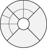
(a) Domain

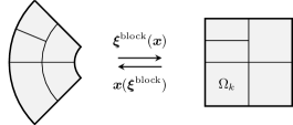
(b) Block

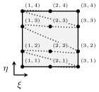
(c) Element $\Omega_{k}$

Figure 1: Top: Geometry of a two-dimensional computational domain composed of four wedge-shaped blocks. Middle: The coordinate transformation $\bm{\xi}^{\mathrm{block}}(\bm{x})$ maps a block to a reference cube in block-logical coordinates $[-1,1]^{2}$. A block is split into elements $\Omega_{k}$ along its logical coordinates axes. Bottom: The element $\Omega_{k}$ in element-logical coordinates $\bm{\xi}=(\xi,\eta)$ with its grid of Legendre-Gauss-Lobatto collocation points. In this example we chose $N_{k,\xi}=3$ and $N_{k,\eta}=4$. Each grid point is labeled with its index $(p_{\xi},p_{\eta})$. The dotted line connects points in the order they are enumerated in by the index $p$.

Once we have formulated the equations, we choose a computational domain on which to discretize them. We decompose the $d$-dimensional computational domain $\Omega\subset\mathbb{R}^{d}$ into a set of blocks shaped like deformed cubes, as illustrated in Fig. 1a. Blocks do not overlap, but they share boundaries. Each face of a block is either shared with precisely one other block, or is external. For example, the domain depicted in Fig. 1a has four wedge-shaped blocks. Each block $B\subset\Omega$ carries a map from the coordinates $\bm{x}\in B$, in which the elliptic equations (2) are formulated, to block-logical coordinates $\bm{\xi}^{\mathrm{block}}\in[-1,1]^{d}$ representing the $d$-dimensional reference cube, as illustrated in Fig. 1b.

Blocks decompose into elements $\Omega_{k}\subset\Omega$, by recursively splitting in half along any of their logical coordinate axes ($h$ refinement). We limit the $h$ refinement of our computational domain such that an element shares its boundary with at most two neighbors per dimension in every direction (“two-to-one balance”), both within a block and across block boundaries. Each element defines element-logical coordinates $\bm{\xi}\in[-1,1]^{d}$ by an affine transformation of the block-logical coordinates. The resulting coordinate map to the reference cube of the element is characterized by the Jacobian

$$\mathrm{J}^{i}_{j}=\partialderivative{{x^{i}}}{{\xi^{j}}}$$ (6)

with determinant $\mathrm{J}$ and inverse ${(\mathrm{J}^{-1})}^{j}_{i}=\partial\xi^{j}/\partial x^{i}$.

On the reference cube of the element we choose a regular grid of collocation points along the logical coordinate axes, as illustrated in Fig. 1c ($p$ refinement). Specifically, we choose $N_{k,i}$ Legendre-Gauss-Lobatto (LGL) collocation points, $\xi_{p_{i}}$, in each dimension $i$, where the index $p_{i}\in\{1,\ldots,N_{k,i}\}$ identifies the grid point along dimension $i$. We also enumerate all $N_{k}=\prod_{i}N_{k,i}$ $d$-dimensional grid points $\bm{\xi}_{p}=(\xi_{p_{1}},\ldots,\xi_{p_{d}})$ in an element with a single index $p\in\{1,\ldots,N_{k}\}$, as illustrated in Fig. 1c.

Then, fields are represented numerically by their values at the collocation points. We denote the set of discrete field values within an element $\Omega_{k}$ as $\underline{u}^{(k)}=(u_{1},\ldots,u_{N_{k}})$, and the collection of discrete field values over all elements as $\underline{u}$. The field values at the collocation points within an element define a $d$-dimensional Lagrange interpolation,

$$u^{(k)}(\bm{x})\coloneqq\sum_{p=1}^{N_{k}}u_{p}\psi_{p}(\bm{\xi}(\bm{x}))\quad\text{with}\quad\bm{x}\in\Omega_{k}\text{,}$$ (7)

where the basis functions $\psi_{p}(\bm{\xi})$ are products of Lagrange polynomials,

$$\psi_{p}(\bm{\xi})\coloneqq\prod_{i=1}^{d}\ell_{p_{i}}(\xi^{i})\quad\text{with}\quad\bm{\xi}\in[-1,1]^{d}\text{.}$$ (8)

based on the collocation points in dimension $i$ of the element. Since Eqs. 7 and 8 are local to each element, fields over the entire domain are discontinuous across element boundaries.

Finally, we employ the strong discontinuous Galerkin scheme developed in Ref. [40] to discretize the equations in first-order flux form, Eq. 2. To compute the matrix-vector product in Eq. 1 we first compute the auxiliary variables $v_{A}$, given the primal variables $u_{A}$, as

$$v_{A}=D_{i}\cdot\tensor{\mathcal{F}}{{}_{\!{v_{A}}}^{i}}+L\cdot((n_{i}\tensor{\mathcal{F}}{{}_{\!{v_{A}}}^{i}})^{*}-n_{i}\tensor{\mathcal{F}}{{}_{\!{v_{A}}}^{i}})-\tilde{\mathcal{S}}_{v_{A}}\text{,}$$ (9a)

where we assume the auxiliary sources can be written in the form $$\mathcal{S}_{v_{A}}=v_{A}+\tilde{\mathcal{S}}_{v_{A}}[u_{A};\bm{x}] f_{v_{A}}=0 v_{A} u_{A}$$ such that Eq. 9a depends only on the primal variables. We also assume for convenience. All elliptic equations that we consider in this article fulfill these assumptions. In a second step, we use the computed auxiliary variables , as well as the primal variables , to compute the DG residuals

$$-M\!\!D_{i}\cdot\tensor{\mathcal{F}}{{}_{\!{u_{A}}}^{i}}-M\!\!L\cdot((n_{i}\tensor{\mathcal{F}}{{}_{\!{u_{A}}}^{i}})^{*} -n_{i}\tensor{\mathcal{F}}{{}_{\!{u_{A}}}^{i}})$$

$$+M\cdot\mathcal{S}_{u_{A}}=M\cdot f_{u_{A}}\text{.}$$ (9b)

The operation $\cdot$ in Eq. 9 denotes a matrix multiplication with the field values over the computational grid of an element. We make use of the mass matrix

$$M_{pq} =\int_{[-1,1]^{d}}\psi_{p}(\bm{\xi})\psi_{q}(\bm{\xi})\sqrt{g}\,\mathrm{J}\differential{{}^{d}\xi}\text{,}$$ (10)

the stiffness matrix

$$M\!\!D_{i,pq} =\int_{[-1,1]^{d}}\psi_{p}(\bm{\xi})\,\partialderivative{\psi_{q}}{{\xi^{j}}}\!(\bm{\xi})\,{(\mathrm{J}^{-1})}^{j}_{i}\sqrt{g}\,\mathrm{J}\differential{{}^{d}\xi}\text{,}$$ (11)

and the lifting operator

$$M\!\!L_{pq} =\int_{[-1,1]^{d-1}}\psi_{p}(\bm{\xi})\psi_{q}(\bm{\xi})\sqrt{{g}^{\Sigma}}\,{\mathrm{J}}^{\Sigma}\differential{{}^{d-1}\xi}$$ (12)

on the element $\Omega_{k}$, as well as the associated ”massless” operators $D_{i}\coloneqq M^{-1}M\!\!D_{i}$ and $L\coloneqq M^{-1}M\!\!L$. Here, $\sqrt{g}$ denotes the determinant of the metric on which the elliptic equations are formulated, such as the conformal metric $\bar{\gamma}_{ij}$ in the XCTS equations (4). The integral in Eq. 12 is over the boundary of the element, $\partial\Omega_{k}$, where $n_{i}$ is the outward-pointing unit normal one-form, ${g}^{\Sigma}$ is the surface metric determinant induced by the background metric, and ${\mathrm{J}}^{\Sigma}$ is the determinant of the surface Jacobian.

The quantities $(n_{i}\tensor{\mathcal{F}}{{}_{\!{v_{A}}}^{i}})^{*}$ and $(n_{i}\tensor{\mathcal{F}}{{}_{\!{u_{A}}}^{i}})^{*}$ in Eq. 9 denote a numerical flux that couples grid points across nearest-neighbor element boundaries. We employ the generalized internal-penalty numerical flux developed in Ref. [40],

$$(n_{i}\tensor{\mathcal{F}}{{}_{\!{v_{A}}}^{i}})^{*}=\frac{1}{2}\Bigl{[} n_{i}^{\mathrm{int}}\tensor{\mathcal{F}}{{}_{\!{v_{A}}}^{i}}(u_{A}^{\mathrm{int}})-n_{i}^{\mathrm{ext}}\tensor{\mathcal{F}}{{}_{\!{v_{A}}}^{i}}(u_{A}^{\mathrm{ext}})\Bigr{]}\text{,}$$ (13a)

$$(n_{i}\tensor{\mathcal{F}}{{}_{\!{u_{A}}}^{i}})^{*}=\frac{1}{2}\Bigl{[} n_{i}^{\mathrm{int}}\tensor{\mathcal{F}}{{}_{\!{u_{A}}}^{i}}\bigl{(}\partial_{j}\tensor{\mathcal{F}}{{}_{\!{v_{A}}}^{j}}(u_{A}^{\mathrm{int}})-\tilde{\mathcal{S}}_{v_{A}}(u_{A}^{\mathrm{int}})\bigr{)}$$

$$-n_{i}^{\mathrm{ext}}\tensor{\mathcal{F}}{{}_{\!{u_{A}}}^{i}}\bigl{(}\partial_{j}\tensor{\mathcal{F}}{{}_{\!{v_{A}}}^{j}}(u_{A}^{\mathrm{ext}})-\tilde{\mathcal{S}}_{v_{A}}(u_{A}^{\mathrm{ext}})\bigr{)}\Bigr{]}$$

$$-\sigma\Bigl{[} n_{i}^{\mathrm{int}}\tensor{\mathcal{F}}{{}_{\!{u_{A}}}^{i}}\bigl{(}n_{j}^{\mathrm{int}}\tensor{\mathcal{F}}{{}_{\!{v_{A}}}^{j}}(u_{A}^{\mathrm{int}})\bigr{)}$$

$$-n_{i}^{\mathrm{ext}}\tensor{\mathcal{F}}{{}_{\!{u_{A}}}^{i}}\bigl{(}n_{j}^{\mathrm{ext}}\tensor{\mathcal{F}}{{}_{\!{v_{A}}}^{j}}(u_{A}^{\mathrm{ext}})\bigr{)}\Bigr{]}$$ (13b)

with the penalty function

$$\sigma=C\,\frac{\big{(}\max(p^{\mathrm{int}},p^{\mathrm{ext}})+1\big{)}^{2}}{\min(h^{\mathrm{int}},h^{\mathrm{ext}})}\text{.}$$ (14)

Here, $u_{A}^{\mathrm{int}}$ denotes the primal variables on the interior side of an element’s shared boundary with a neighbor, and $u_{A}^{\mathrm{ext}}$ denotes the primal variables on the neighbor’s side, i.e., the exterior. Note that $n_{i}^{\mathrm{ext}}=-n_{i}^{\mathrm{int}}$ for the purpose of this article, since we only consider equations formulated on a fixed background metric, but the scheme does not rely on this assumption. For Eq. 14 we also make use of the polynomial degree $p$, and a measure of the element size, $h$, orthogonal to the element boundary on either side of the interface, as detailed in Ref. [40].

We impose boundary conditions through fluxes, i.e., by a choice of exterior quantities in the numerical flux, Eq. 13. Specifically, on external boundaries we set

$$(n_{i}\tensor{\mathcal{F}}{{}_{\!{\alpha}}^{i}})^{\mathrm{ext}}=(n_{i}\tensor{\mathcal{F}}{{}_{\!{\alpha}}^{i}})^{\mathrm{int}}-2(n_{i}\tensor{\mathcal{F}}{{}_{\!{\alpha}}^{i}})^{\mathrm{b}}\text{,}$$ (15)

where we choose the boundary fluxes $(n_{i}\tensor{\mathcal{F}}{{}_{\!{\alpha}}^{i}})^{\mathrm{b}}$ depending on the boundary conditions we intend to impose. For Neumann-type boundary conditions we choose the primal boundary fluxes $(n_{i}\tensor{\mathcal{F}}{{}_{\!{u_{A}}}^{i}})^{\mathrm{b}}$ directly, e.g., $(n_{i}\tensor{\mathcal{F}}{{}_{\!{\varphi}}^{i}})^{\mathrm{b}}=n_{i}\partial_{i}\varphi|_{\mathrm{b}}$ for the Maxwell constraint (1), and set the auxiliary boundary fluxes to their interior values, $(n_{i}\tensor{\mathcal{F}}{{}_{\!{v_{A}}}^{i}})^{\mathrm{b}}=(n_{i}\tensor{\mathcal{F}}{{}_{\!{v_{A}}}^{i}})^{\mathrm{int}}$. For Dirichlet-type boundary conditions we choose the primal boundary fields $u_{A}^{\mathrm{b}}$, e.g., $\varphi|_{\mathrm{b}}$ for the Maxwell constraint (1), to compute the auxiliary boundary fluxes $(n_{i}\tensor{\mathcal{F}}{{}_{\!{v_{A}}}^{i}})^{\mathrm{b}}=n_{i}^{\mathrm{b}}\tensor{\mathcal{F}}{{}_{\!{v_{A}}}^{i}}(u_{A}^{\mathrm{b}})$, and set the primal boundary fluxes to their interior values, $(n_{i}\tensor{\mathcal{F}}{{}_{\!{u_{A}}}^{i}})^{\mathrm{b}}=(n_{i}\tensor{\mathcal{F}}{{}_{\!{u_{A}}}^{i}})^{\mathrm{int}}$.

In summary, the DG residuals (9) are algebraic equations for the discrete primal field values $\underline{u}_{A}$ on all elements and grid points in the computational domain. For linear PDEs, the left-hand side of Eq. 9 defines a matrix-vector product with a set of primal field values on the computational domain. The right-hand side of Eq. 9 is a set of fixed values on the computational domain. Therefore, Eq. 9 has the form of Eq. 1.

III Task-based iterative algorithms

Once the elliptic problem is discretized, it is the responsibility of the elliptic solver to invert the matrix equation (1) numerically, in order to obtain the solution vector $\underline{u}$ over the computational grid. For large problems on high-resolution grids it is typically unfeasible to invert the matrix $\mathcal{A}$ in Eq. 1 directly, or even to explicitly construct and store it. Instead, we employ iterative algorithms that require only the matrix-vector product $\mathcal{A}\underline{u}$ be defined, and that parallelize to computing clusters.

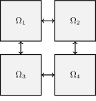
(a) Domain

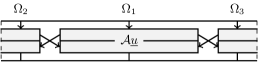
(b) Tasks

Figure 2: Parallelization structure of the matrix-vector product $\mathcal{A}\underline{u}$. Top: Decomposition of a two-dimensional rectangular domain into four elements. Arrows illustrate the dependence between nearest-neighbor elements to compute the matrix-vector product $\mathcal{A}\underline{u}$. Bottom: Tasks involved to compute the matrix-vector product $\mathcal{A}\underline{u}$. Each element performs a task that prepares and sends data to its neighbors (upper half of the rectangle), and another that receives data from its neighbors and performs the computation (lower half of the rectangle). The arrows between elements are the same as in the top panel.

The discontinuous Galerkin (DG) matrix-vector product $\mathcal{A}\underline{u}$ is well suited for parallelization. As Sec. II summarized, it decomposes into a set of operations local to the elements that make up the computational domain. Figure 2 illustrates a computational domain composed of elements, as well as the dependence of the elements on each other for computing the matrix-vector product. The matrix-vector product requires only data local to each element and on both sides of the boundary that the element shares with its nearest neighbors. Therefore, it can be computed in parallel, and requires only a single communication between each pair of nearest-neighbor elements to exchange data on their shared boundary. The matrix-vector product acts as a “soft” global synchronization point, meaning that it requires all elements have sent data to their neighbors before all elements can proceed with the algorithm, but individual elements can already proceed once they receive data from their nearest neighbors.

The decomposition of the domain into elements also admits a strategy to distribute computation across the processors of the computer system. We distribute elements among the available cores in a way that, ideally, minimizes the number of internode communications and assigns an equal amount of work to each core. In this article we employ a Morton (“z-order”) space-filling curve [41] to traverse the elements within a block of the computational domain and fill up the available cores. We weight the elements by their number of grid points to approximately balance the amount of work assigned to each core. With this strategy, neighboring elements tend to lie on the same node, though more effective element-distribution and load-balancing strategies based on, for example, Hilbert space-filling curves [42] are a subject of future work.

Once elements have been assigned to the available cores, each element traverses the list of tasks in the algorithm. When it encounters a task whose dependencies are not yet fulfilled, e.g., when neighbors have not yet sent the data on shared boundaries needed for the DG matrix-vector product, the element relinquishes control of the core to another whose dependencies are fulfilled. Reference [30] describes SpECTRE’s task-based parallel runtime system based on the Charm++ [38] framework in more detail.

Figure 3: Overview of the technology stack we employ to solve the discretized elliptic problem (1). All algorithms above the dotted line follow SpECTRE’s task-based parallelism paradigm. The algorithms below the dotted line run within a task, and on all elements independently.

Figure 3 provides an overview of the algorithms that we employ to iteratively solve the discretized elliptic problem (1), with details given in subsequent sections: nonlinear equations are linearized with a Newton-Raphson scheme with a line-search globalization (Sec. III.1). The resulting linear subproblems are solved with an iterative Krylov-subspace method (Sec. III.2), preconditioned with a multigrid solver (Sec. III.3). On every level of the multigrid hierarchy we run a few iterations of an additive Schwarz smoother, which solves the problem approximately on independent, overlapping, element-centered subdomains (Sec. III.4). Each subdomain problem is solved by another Krylov-type method, which carries a Laplacian-approximation preconditioner with an incomplete LU explicit-inversion scheme to accelerate the solve (Sec. III.5). All algorithms are implemented in the open-source SpECTRE code and take advantage of its task-based parallel infrastructure [29, 30].

III.1 Newton-Raphson nonlinear solver

The Newton-Raphson scheme iteratively refines an initial guess $\underline{u}_{0}$ for a nonlinear problem $\mathcal{A}(\underline{u})=\underline{b}$ by repeatedly solving the linearized problem

$$\frac{\delta\mathcal{A}}{\delta u}(\underline{u})\,\Delta\underline{u}=\underline{b}-\mathcal{A}(\underline{u})$$ (16)

for the correction $\Delta\underline{u}$, and then updating the solution as $\underline{u}\rightarrow\underline{u}+\Delta\underline{u}$ [43, 44].

The Newton-Raphson method converges quadratically once it reaches a basin of attraction, but can fail to converge when the initial guess is too far from the solution. We employ a line-search globalization strategy to recover convergence in such cases, following Alg. 6.1.3 in Ref. [44]. It iteratively reduces the step length $\lambda$ until the corrected residual $\lVert\underline{b}-\mathcal{A}(\underline{u}+\lambda\Delta\underline{u})\rVert_{2}$ has sufficiently decreased, meaning it has decreased by a fraction of the predicted decrease if the problem was linear. This fraction is the sufficient-decrease parameter controlling the line search. The line search typically starts at ${\lambda=1}$ in every Newton-Raphson iteration, but the initial step length can be decreased to dampen the nonlinear solver. Although the line-search globalization has proven effective for the cases we have encountered so far, alternative globalization strategies such as a trust-region method or more sophisticated nonlinear preconditioning techniques can be investigated in the future.

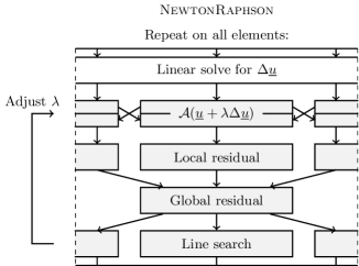
Figure 4: Parallelization structure of the task-based Newton-Raphson nonlinear solver (Sec. III.1).

Figure 4 illustrates our task-based implementation of the Newton-Raphson algorithm. The sufficient-decrease condition, and the necessity to check the global residual magnitude against convergence criteria, introduce a synchronization point in the form of a global reduction to assemble the residual magnitude $\lVert\underline{b}-\mathcal{A}(\underline{u}+\lambda\Delta\underline{u})\rVert_{2}$. The algorithm requires one nonlinear operator application $\mathcal{A}(\underline{u}+\lambda\Delta\underline{u})$ per iteration, plus one additional nonlinear operator application for every globalization step that reduces the step length. Since a typical nonlinear elliptic solve requires $\lesssim 10$ Newton-Raphson iterations, the parallelization properties of this algorithm are not particularly important for the overall performance.

Exactly once per iteration the Newton-Raphson algorithm dispatches a linear solve of Eq. 16 for the correction $\Delta\underline{u}$. This iterative linear-solver algorithm is the subject of the following section.

III.2 Krylov-subspace linear solver

We solve the linearized problem (16) with an iterative Krylov-subspace algorithm. We generally employ a GMRES algorithm, but have also developed a conjugate gradients algorithm for discretized problems that are symmetric positive definite [47, 48]. These algorithms solve a linear problem $\mathcal{A}\underline{u}=\underline{b}$ iteratively by building up a basis of the Krylov subspace $K_{k}=\left\{\underline{b},\mathcal{A}\underline{b},\mathcal{A}^{2}\underline{b},\ldots,\mathcal{A}^{k-1}\underline{b}\right\}$. Krylov-subspace algorithms are guaranteed to find a solution in at most $N_{\mathrm{DOF}}$ iterations, where $N_{\mathrm{DOF}}$ is the size of the matrix $\mathcal{A}$.

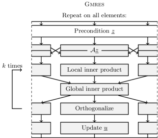
Figure 5: Parallelization structure of the task-based GMRES Krylov-subspace linear solver (Sec. III.2).

Figure 5 illustrates our task-based GMRES algorithm, which is based on Alg. 9.6 in Ref. [48]. It requires one application of the linear operator $\mathcal{A}$ per iteration. Then, the algorithm is characterized by an Arnoldi orthogonalization procedure to construct a new basis vector $\underline{z}$ of the Krylov subspace that is orthogonal to all previously constructed basis vectors. The orthogonalization procedure requires a global reduction to assemble the inner product of the new basis vector with every existing basis vector, meaning the GMRES algorithm needs to perform $k$ reductions in the $k$th iteration. Every reduction constitutes a global synchronization point, since it requires that all elements send data to a single core on the computer system and wait for a broadcast from that core back to all elements. A conjugate gradients algorithm also requires a global reduction per iteration, but avoids the additional reductions from the orthogonalization procedure.

Due to the global synchronization points involved in every iteration of the Krylov-subspace solver, it is essential to keep the number of iterations to a minimum in order to achieve good parallel performance. To this end, we invoke a preconditioner in every iteration of the Krylov-subspace algorithm and place particular focus on its parallelization properties. The preconditioner is responsible for solving the linear problem approximately to accelerate the convergence of the Krylov-subspace algorithm. Effective parallel preconditioning techniques for our DG-discretized elliptic problems are the main focus of this article. Since we employ the flexible variant of the GMRES algorithm, the preconditioner may change between iterations [48]. While the flexible GMRES algorithm with a variable preconditioner is not mathematically guaranteed to converge in at most $N_{\mathrm{DOF}}$ iterations anymore, in practice, it converges in much fewer than $N_{\mathrm{DOF}}$ iterations (see test problems in Sec. IV, in particular Figs. 12 and 15).

Typically, the number of iterations needed by an unpreconditioned Krylov-subspace algorithm increases with the size of the problem. The convergence behavior is often connected to the condition number of the linear operator,

$$\kappa=\frac{\lambda_{\mathrm{max}}}{\lambda_{\mathrm{min}}}\text{,}$$ (17)

where $\lambda_{\mathrm{max}}$ and $\lambda_{\mathrm{min}}$ denote the largest and smallest eigenvalue of the matrix, respectively. However, note that rigorous convergence bounds for the GMRES algorithm in terms of the condition number exist only when the matrix is normal [48]. Nevertheless, the condition number can provide an indication for the expected rate of convergence. For the discontinuous Galerkin discretization we employ in this article, the condition number scales as $\kappa\propto p^{2}/h$, where $p$ denotes a typical polynomial degree of the elements and $h$ denotes a typical element size [40, 39, 49, 50]. This scaling is related to the decrease of the minimum spacing between Legendre-Gauss-Lobatto collocation points, which scales quadratically with $p$ near element boundaries and linearly with the element size.

More specifically, Krylov-subspace methods struggle to solve large-scale modes in the solution. The algorithm solves modes on the scale of the grid-point spacing or the size of elements in just a few iterations, but it needs a lot more iterations to solve modes spanning the full domain. Such large-scale modes carry, for example, information from boundary conditions that must traverse the entire domain. The test problem presented in Fig. 11 below illustrates this effect. Therefore, we precondition the Krylov-subspace solver with a multigrid algorithm that uses information from coarser grids, where the large-scale modes from finer grids become small scale.

III.3 Multigrid preconditioner

We employ a geometric V/̄cycle multigrid algorithm, as prototyped in Ref. [39]. Our multigrid solver can be used standalone, or to precondition a Krylov-type linear solver as described in Sec. III.2 (“Krylov-accelerated multigrid”).

III.3.1 Grid hierarchy

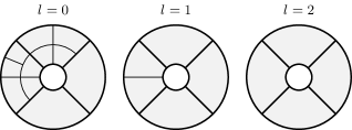
Figure 6: Multigrid hierarchy based on the domain depicted in Fig. 1a.

The geometric multigrid algorithm relies on a strategy to coarsen the computational grid. We primarily $h$-coarsen the domain, meaning that we create multigrid levels $l>0$ by successively combining two elements into one along every dimension of the grid, as illustrated in Fig. 6. We only $p$-coarsen the grid in the sense that we choose the smaller of the two polynomial degrees when combining elements along an axis. This strategy follows Ref. [39] and ensures that coarse-grid field approximations always have an exact polynomial representation on finer grids.

The coarsest possible grid that our domain decomposition can achieve has a single element per block that make up the domain. For example, the two-dimensional shell depicted in Fig. 6 has four wedge-shaped blocks, each of which is a deformed cube. Our multigrid algorithm works best when the domain is composed of as few blocks as possible.

III.3.2 Intermesh operators

To project data between grids we use the standard $L_{2}$-projections (or Galerkin projections) detailed in Ref. [40]. Fields on coarser grids are projected to finer grids with the prolongation operator

$$P_{\tilde{p}p}^{\,l+1\rightarrow l}=\prod_{i=1}^{d}\ell_{p_{i}}(\tilde{\xi}_{\tilde{p}_{i}})\text{,}$$ (18)

where $p$ enumerates grid points on the coarser grid, $\tilde{p}$ enumerates grid points on the finer grid, and $\tilde{\xi}_{\tilde{p}_{i}}$ are the coarse-grid logical coordinates of the fine-grid collocation points. For fine-grid (child) elements that cover the full coarse-grid (parent) element in dimension $i$ the coarse-grid logical coordinates are just the fine-grid collocation points, $\tilde{\xi}_{\tilde{p}_{i}}=\xi_{\tilde{p}_{i}}$. For child elements that cover the lower or upper logical half of the parent element in dimension $i$ they are $\tilde{\xi}_{\tilde{p}_{i}}=(\xi_{\tilde{p}_{i}}-1)/2$ or $\tilde{\xi}_{\tilde{p}_{i}}=(\xi_{\tilde{p}_{i}}+1)/2$, respectively. Note that the prolongation operator (18) is just a Lagrange interpolation from the coarser to the finer grid. The interpolation retains the accuracy of the polynomial approximation because the finer grid always has sufficient resolution.

To project data from finer to coarser grids we employ the restriction operator

$$R^{\,l\rightarrow l+1}=(P^{\,l+1\rightarrow l})^{T}\text{,}$$ (19)

which is the transpose of the prolongation operator (18). Contrary to the restriction operator listed in Ref. [40] the multigrid restriction involves no mass matrices because it applies to DG residuals, Eq. 9, which already include mass matrices.

III.3.3 Algorithm

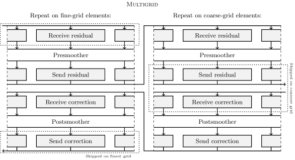
Figure 7: Parallelization structure of the task-based multigrid algorithm (Sec. III.3). Elements on all grids perform the same set of tasks, with some tasks skipped on the finest grid and other tasks skipped on the coarsest grid.

Figure 7 illustrates our task-based implementation of the multigrid V/̄cycle algorithm to solve linear problems $\mathcal{A}\underline{u}=\underline{b}$. On every grid $l$ we approximately solve the linear problem

$$\mathcal{A}_{l}\,\underline{u}^{(l)}=\underline{b}^{(l)}\text{,}$$ (20)

where the operator $\mathcal{A}_{l}$ is the discretization of the elliptic PDEs on the grid $l$. At the beginning of a V/̄cycle, on the finest grid $l=0$, we select $\underline{u}^{(0)}=\underline{u}$ and $\underline{b}^{(0)}=\underline{b}$; hence, approximately solving the original linear problem (“presmoothing”). Then, the remaining residual

$$\underline{r}^{(l)}=\underline{b}^{(l)}-\mathcal{A}_{l}\,\underline{u}^{(l)}$$ (21)

is restricted to source the linear problem (20) on the next-coarser grid,

$$\underline{b}^{(l+1)}=R^{\,l\rightarrow l+1}\,\underline{r}^{(l)}\text{.}$$ (22)

Once presmoothing is complete on the coarsest grid (the “tip” of the V/̄cycle), we approximately solve Eq. 20 again (“postsmoothing”). The solution of the postsmoothing step is prolongated to the next-finer grid as a correction,

$$\underline{u}^{(l)}\quad\leftarrow\quad\underline{u}^{(l)}+P^{\,l+1\rightarrow l}\,\underline{u}^{(l+1)}\text{.}$$ (23)

Prolongation, correction, and postsmoothing proceed until we have returned to the finest grid, where the correction and postsmoothing apply to the original linear problem. Our choice of presmoother and postsmoother to approximately solve Eq. 20 is detailed in Sec. III.4 below. Note that on the coarsest level we apply both presmoothing and postsmoothing.

The restriction of residuals to the next-coarser grid and the prolongation of corrections to the next-finer grid incur soft synchronization points. Specifically, only once all elements on the finer grid have restricted their residuals to the coarser grid can all elements on the coarser grid proceed, though individual coarse-grid (parent) elements can already proceed once only their corresponding fine-grid (child) elements have sent the restricted residuals. The same applies to the prolongation of corrections from the parent elements back to their children. Therefore, parent elements on coarser grids ideally follow their children when distributed among the available cores, initially and at load-balancing operations.

In contrast to Krylov-subspace algorithms, the multigrid algorithm involves no global synchronization points. In particular, for diagnostic output we perform a reduction to compute the global residual norm $\lVert\underline{r}^{(l)}\rVert$ on every grid, but do so asynchronously in order to avoid a synchronization that is not algorithmically necessary. Therefore, we do not use the global residual norm as a convergence criterion for the multigrid solver. Instead, we run a fixed number of multigrid V/̄cycles, and typically only a single one to precondition a Krylov-subspace solver.

III.4 Schwarz smoother

On every level of the grid hierarchy the multigrid solver relies on a smoother that approximately solves Eq. 20. In principle, the smoother can be any linear solver, including a Krylov-subspace solver as detailed in Sec. III.2. However, to achieve good parallel performance we have developed a highly asynchronous additive Schwarz smoother [53, 54, 39], that we employ for presmoothing and postsmoothing on every level of the multigrid hierarchy. Note that we also apply it on the coarsest grid, where some authors apply a dedicated bottom smoother instead [55, 56]. Since our coarsest grids are rarely reduced to a single element (see Sec. III.3.1), we have, so far, preferred the asynchronous Schwarz smoother over direct bottom smoothers. Our Schwarz smoother can be used standalone, as a preconditioner for a Krylov-type linear solver, or as a smoother for the multigrid solver (which may, in turn, precondition a Krylov-type solver).

The additive Schwarz method works by solving many subproblems in parallel and combining their solutions as a weighted sum to converge towards the global solution. The decomposition into independent subproblems makes this linear solver very parallelizable. The Schwarz solver is based on our prototype in Ref. [39], with variations to the subdomain geometry and weighting to take better advantage of our task-based parallelism, and with novel subdomain preconditioning techniques.

III.4.1 Subdomain geometry

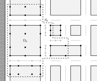
Figure 8: An element-centered subdomain $S_{k}$ with ${N_{\mathrm{overlap}}=2}$ (dashed line) associated with the element $\Omega_{k}$ in a two-dimensional computational domain. The domain is composed of elements (black rectangles) with their mesh of grid points (black dots) and depicted here in block-logical coordinates. The diagonally-shaded region to the left illustrates an external domain boundary. The light gray lines between neighboring element faces illustrate mortar meshes, which are relevant for the subdomain operator in a DG context but play no role in the Schwarz algorithm [40]. Note that the empty space between the elements in this visualization is not part of the computational domain.

We partition the computational domain into overlapping, element-centered subdomains $S_{k}\subset\Omega$, which have a one-to-one association with the DG elements $\Omega_{k}$. Each subdomain $S_{k}$ is centered on the DG element $\Omega_{k}$. It extends by $N_{\mathrm{overlap}}$ collocation points into neighboring elements across every face of $\Omega_{k}$, up to, but excluding, the collocation points on the face of the neighbor pointing away from the subdomain. Fig. 8 illustrates the geometry of our element-centered subdomains.

The subdomain does not extend into corner or edge neighbors, which is a choice different to both Ref. [54] and Ref. [39]. We avoid diagonal couplings because in a DG context information only propagates across faces, as already noted in Ref. [54]. Elimination of the corner and edge neighbors reduces the complexity of the subdomain geometry, the number of communications necessary to exchange data between elements in the subdomain, and hence the connectivity of the dependency graph between tasks. This element-centered subdomain geometry based solely on face neighbors has proven viable for the test problems presented below, and for our task-based parallel architecture.

The one-to-one association between elements and subdomains allows to store all quantities that define the subdomain geometry local to the central element, i.e., on the same core. The same applies to all data on the grid points of the subdomain. Therefore, operations local to the subdomain require no communication, but communication between overlapping elements is necessary to assemble data on the subdomains, and to make data on subdomains available to overlapped elements.

III.4.2 Subdomain restriction

To restrict quantities defined on the full computational domain $\Omega$ to a subdomain $S\subset\Omega$ the Schwarz solver employs a restriction operator $R_{S}$. Since our subdomains are subsets of the grid points in the full computational domain, our restriction operator simply discards all nodal data on grid points outside the subdomain. Similarly, the transpose of the restriction operator, $R_{S}^{T}$, extends subdomain data with zeros on all grid points outside the subdomain.

The Schwarz solver also relies on a restriction of the global linear operator $\mathcal{A}$ to the subdomains. The subdomain operator $\mathcal{A}_{S}$ on a subdomain $S$ is formally defined as $\mathcal{A}_{S}=R_{S}\mathcal{A}R_{S}^{T}$. In practice, it evaluates the same DG matrix-vector product as the full operator $\mathcal{A}$, i.e., the left-hand side of Eq. 9, but assumes that all data outside the subdomain is zero. It performs all interelement operations of the full DG operator, but computes them entirely with data local to the subdomain. Therefore, it requires no communication between cores, as opposed to the global linear operator $\mathcal{A}$ that must communicate data between nearest neighbors for every operator application.

III.4.3 Subdomain problems

On every subdomain $S$ we solve the restricted problem

$$\mathcal{A}_{S}\,\Delta\underline{u}^{(S)}=\underline{r}^{(S)}$$ (24)

for the subdomain correction $\Delta\underline{u}^{(S)}$. Here, $\mathcal{A}_{S}$ is the subdomain operator and $\underline{r}^{(S)}=R_{S}\,\underline{r}$ is the global residual $\underline{r}=\underline{b}-\mathcal{A}\underline{u}$ restricted to the subdomain.

The subdomain problems (24) are solved by means of a subdomain solver, detailed in Sec. III.5. The choice of subdomain solver affects only the performance of the Schwarz algorithm, not its convergence or parallelization properties, assuming the solutions to the subdomain problems (24) are sufficiently precise.

III.4.4 Weighting

Once we have obtained the subdomain correction $\Delta\underline{u}^{(S)}$ on every subdomain $S$, we combine them as a weighted sum to correct the solution,

$$\underline{u}\quad\leftarrow\quad\underline{u}+\sum_{S}R_{S}^{T}\left(\underline{w}^{(S)}\,\Delta\underline{u}^{(S)}\right)\text{,}$$ (25)

where $\underline{w}^{(S)}$ is a weight at every grid point of the subdomain. This is the additive approach of the algorithm, which has the advantage over multiplicative Schwarz methods that all subdomain problems decouple and can be solved in parallel. The weighted sum, Eq. 25, is never assembled globally. Instead, every element adds the contribution from its locally centered subdomain and from all overlapping subdomains to the components of $\underline{u}$ that resides on the element.

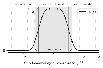
Figure 9: The one-dimensional weight function $w(\xi)$ for the Schwarz solver. Depicted is an element-centered subdomain in one dimension with $N_{\text{overlap}}=2$. Every element has $N_{k}=6$ LGL collocation points, which includes grid points on the shared element boundaries (black vertical lines). The overlap width $\delta$ is the logical coordinate distance to the first point outside the subdomain, where the weight becomes zero.

The weights $\underline{w}^{(S)}$ represent a scalar field on every subdomain, which must be conserved as

$$\sum_{S}R_{S}^{T}\,\underline{w}^{(S)}=\underline{1}\text{.}$$ (26)

We follow Refs. [39, 54] in constructing the weights as quintic smoothstep polynomials, but must account for the missing weight from corner and edge neighbors. Specifically, we compute

$$w^{(S)}_{p}=W(\bm{\xi}^{(S)}_{p})$$ (27)

by evaluating the scalar weight function $W(\bm{\xi})$ at the logical coordinates $\bm{\xi}^{(S)}_{p}$ of the grid points in the subdomain. These subdomain-logical coordinates coincide with the element-logical coordinates of the central element, and extend outside the central element such that $\xi^{(S)}=\pm 3$ coincides with the sides of the overlapped neighbors that face away from the subdomain (see abscissa of Fig. 9). The scalar weight function

$$W(\bm{\xi})=\prod^{d}_{i=0}w(\xi^{i})$$ (28)

is a product of one-dimensional weight functions,

$$w(\xi) =\frac{1}{2}\left(\phi\left(\frac{\xi+1}{\delta}\right)-\phi\left(\frac{\xi-1}{\delta}\right)\right)$$ (29)

$$\text{with}\quad\phi(\xi) =\begin{cases}\frac{1}{8}\left(15\xi-10\xi^{3}+3\xi^{5}\right)&\quad\xi\in[-1,1]\\ \mathrm{sign}(\xi)\quad&\quad|\xi|>1\text{,}\end{cases}$$ (30)

where $\phi(\xi)$ is a second-order smoothstep function, i.e., a quintic polynomial, and $\delta\in(0,2]$ is the overlap width. The overlap width is the logical coordinate distance from the boundary of the central element to the first collocation point outside the overlap region (see Fig. 9). With this definition the overlap width is nonzero even when the overlap extends only to a single LGL point in the neighbor, which coincides with the element boundary. Furthermore, the weight is always zero at subdomain-logical coordinates $\xi^{(S)}=\pm 3$, even for $\delta=2$ when the overlap region covers the full neighbor in width. This is the reason we never include the collocation points on the side of the neighbor facing away from the subdomain (see Sec. III.4.1). Figure 9 illustrates the shape of the weight function.

To account for the missing weight from corner and edge neighbors, we could add it to the central element, to the overlap data from face neighbors, or split it between the two. We choose to add it to the face neighbors that share a corner or edge, since in a DG context that is where the information from those regions propagates through.

III.4.5 Algorithm

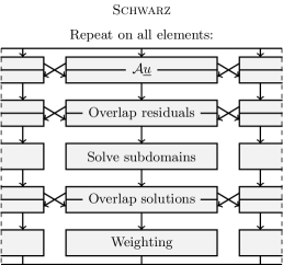
Figure 10: Parallelization structure of the task-based Schwarz smoother (Sec. III.4).

Fig. 10 illustrates our task-based implementation of the additive Schwarz solver. In each iteration, the algorithm computes the residual $\underline{r}=\underline{b}-\mathcal{A}\underline{u}$, restricts it to all subdomains as $\underline{r}^{(S)}=R_{S}\,\underline{r}$, and exchanges it on overlap regions with neighboring elements. Once an element has received all residual data on its subdomain, it solves the subdomain problem, Eq. 24, for the correction $\Delta\underline{u}^{(S)}$. Since all elements perform such a subdomain solve, we end up with a subdomain solution $\Delta\underline{u}^{(S)}$ on every element-centered subdomain, and the solutions overlap. Therefore, the algorithm exchanges the subdomain solutions on overlap regions with neighboring elements and adds them to the solution field $\underline{u}$ as the weighted sum, Eq. 25.

In order to compute the residual $\underline{r}$ that is restricted to the subdomains to serve as source for the subdomain solves, we must apply the global linear operator $\mathcal{A}$ to the solution field $\underline{u}$ once per Schwarz iteration. This operator application, as well as the steps to communicate the residuals and the solutions on overlaps, incur soft synchronization points through nearest-neighbor couplings. However, once the residuals on overlaps are communicated, all subdomain solves are independent of each other. This constitutes the main source of parallelization in the elliptic solver.

The subdomain solves not only run in parallel, but also scale with the problem size. Increasing the number of grid points in the elements ($p$ refinement) makes the subdomain solves more expensive, but the effectiveness of a Schwarz iteration ideally remains the same. Increasing the number of elements ($h$ refinement) leads to more subdomain solves that can run in parallel. The Schwarz solver does not resolve large-scale modes, so Krylov-type solvers still rely on the multigrid algorithm to scale with $h$ refinement.

III.5 Subdomain solver

Once overlapping subdomains have exchanged data we can solve all subdomain problems (24) in parallel with data local to each subdomain. Since the subdomain operator $\mathcal{A}_{S}$ is defined as a matrix-vector product, we solve Eq. 24 with a preconditioned GMRES algorithm, or with conjugate gradients for symmetric positive definite problems. The algorithm is the same as detailed in Sec. III.2 for our task-based parallel Krylov-subspace linear solver, but implemented separately as a serial algorithm. In future work, we may opt to parallelize the subdomain solver over a few threads with shared memory, but currently we prefer to employ the available cores to solve multiple subdomain problems in parallel. In particular, on coarse multigrid levels where the number of elements can be smaller than the number of available cores, parallelizing the subdomain solves over otherwise idle cores may increase performance.

The iterative Krylov subdomain solves constitute the majority of the total computational expenses, so a suitable preconditioner for them can speed up the elliptic solve significantly. To our knowledge, preconditioners for Schwarz subdomain solvers have gotten little attention in the literature so far. In some cases, the discretization scheme allows to construct a matrix representation for the subdomain operator explicitly, making it possible to invert it directly with little effort [54]. In other cases, the subdomain operator is small enough to build the matrix representation column-by-column (see Sec. III.5.2), e.g., when solving the Poisson equation. However, when solving sets of coupled elliptic equations the subdomain operator can easily become too large to construct explicitly. For example, the subdomain operator for the XCTS equations (4) (five variables) on a three-dimensional grid with $8^{3}$ grid points per element and $N_{\mathrm{overlap}}=2$ is a matrix of size $6400\times 6400$. Stored densely, it requires over $300\text{\,}\mathrm{MB}$ of memory per element, so typical contemporary computing clusters with a few $\mathrm{GB}$ of memory per core could only hold a few elements per core. Sparse storage reduces the memory cost significantly, but still requires $6400$ subdomain-operator applications to construct the matrix representation and a nonnegligible cost to invert and to apply it. With an iterative Krylov-subspace algorithm and a suitable preconditioner we can solve the subdomain problems on an element with significantly lower cost and memory requirements. For example, test problem IV.2 completes about an order of magnitude faster with the subdomain preconditioner laid out in this section, than with an unpreconditioned GMRES subdomain solver.

III.5.1 Laplacian-approximation preconditioner

We support the iterative subdomain solver with a Laplacian-approximation preconditioner. It approximates the linearized elliptic PDEs with a Poisson equation for every variable. A similar preconditioning strategy has proven successful for the SpEC code [14], but in the context of a spectral discretization scheme and a very different linear-solver stack. Specifically, we approximate the subdomain problem, Eq. 24, as a set of independent Poisson subdomain problems

$$\mathcal{A}^{\mathrm{Poisson}}_{S}\,\Delta\underline{u}^{(S)}_{A}=\underline{r}^{(S)}_{A}\text{,}$$ (31)

where the index $A$ iterates over all primal variables (see Sec. II). Here, $\mathcal{A}^{\mathrm{Poisson}}_{S}$ is the DG-discretization of the negative Laplacian $-g^{ij}\nabla_{i}\nabla_{j}$ on the subdomain according to Sec. II. For example, a three-dimensional XCTS problem has five variables, so Eq. 31 approximates the linearization (16) of the five equations (4) as

$$\bar{\nabla}^{2}\delta\psi=0\text{,}\quad\bar{\nabla}^{2}\delta(\alpha\psi)=0\quad\text{and}\quad\bar{\nabla}^{2}\delta\beta^{i}=0\text{.}$$ (32)

Depending on the elliptic system at hand we either choose a flat background metric $g_{ij}=\delta_{ij}$, or the background metric of the elliptic system, such as the conformal metric $g_{ij}=\bar{\gamma}_{ij}$ for an XCTS system. A curved background metric reduces the sparsity of the Poisson operator but approximates the elliptic equations better. In practice, we have found little difference in runtime between the flat-space and curved-space Laplacian approximations.

We choose homogeneous Dirichlet or Neumann boundary conditions for $\mathcal{A}^{\mathrm{Poisson}}_{S}$. For variables and element faces where the original boundary conditions are of Dirichlet type we choose homogeneous Dirichlet boundary conditions, and for those where the original boundary conditions are of Neumann type we choose homogeneous Neumann boundary conditions. This may lead to more than one distinct Poisson operator on subdomains with external boundaries, one per unique combination of element face and boundary-condition type among the variables. Subdomains that have exclusively internal boundaries only ever have a single Poisson operator, which applies to all variables. Note that the choice of homogeneous boundary conditions for the Poisson subdomain problems is compatible with inhomogeneous boundary value problems, because the inhomogeneity in the boundary conditions is absorbed in the fixed sources when the equations are linearized [40].

To solve the Poisson subdomain problems (31), one per variable, we can (again) employ any choice of linear solver, such as a (preconditioned) Krylov-subspace algorithm. However, at this point we have reduced the full elliptic problem down to a single Poisson problem limited to a subdomain that is solved for all variables, or a few Poisson problems on subdomains with external boundaries. Therefore, it becomes feasible, and indeed worthwhile, to construct the Poisson subdomain-operator matrix explicitly and to invert it directly. In particular, the approximate Poisson subdomain-operator matrix remains valid throughout the full nonlinear elliptic solve, as long as the grid, the background metric, and the type of boundary conditions remain unchanged, so that its construction cost is amortized over many applications.

III.5.2 Explicit-inverse solver

We solve the Poisson subproblems of the Laplacian-approximation preconditioner, Eq. 31, with an explicit-inverse solver. It constructs the matrix representation of a linear subdomain operator $\mathcal{A}_{S}$ column-by-column, and then inverts it directly by means of an LU decomposition. Once the inverse $\mathcal{A}_{S}^{-1}$ has been constructed, each subdomain problem $\mathcal{A}_{S}\,\Delta\underline{u}^{(S)}=\underline{r}^{(S)}$ is solved by a single application of the inverse matrix,

$$\Delta\underline{u}^{(S)}=\mathcal{A}_{S}^{-1}\,\underline{r}^{(S)}\text{.}$$ (33)

This means that subdomains have a large initialization cost, but fast repeated solves.

When the explicit-inverse solver is employed as a preconditioner, e.g., to solve the individual Poisson problems of the Laplacian-approximation preconditioner (Sec. III.5.1), the inverse does not need to be exact. Therefore, we construct an incomplete LU decomposition with a configurable fill-in and store it in sparse format. Then, each subdomain problem reduces to two sparse triangular matrix solves. We use the Eigen [57] sparse linear algebra library for the incomplete LU decomposition, which uses the ILUT algorithm [58]. The Poisson subdomain-operator matrices $\mathcal{A}_{S}^{\mathrm{Poisson}}$ have a sparsity of about $90\text{\,}\mathrm{\char 37\relax}$, which translates to a sparsity of about $90\text{\,}\mathrm{\char 37\relax}$ for the incomplete LU decomposition as well, since we use a fill-in factor of one. The sparsity of the inverse reduces the computational cost for applying it to every subdomain problem, as well as the memory required to store the inverse.

Note that the explicit matrix must be reconstructed when the linear operator changes. The Poisson operators of the Laplacian-approximation preconditioner do not typically change, which makes the explicit-inverse solver very effective (see Sec. III.5.1). However, in case we apply the explicit-inverse solver to the full subdomain problem directly, the linearized operator typically changes between every outer nonlinear solver iteration. In such cases, we can choose to skip the reconstruction of the explicit matrix to avoid the computational expense, at the cost of losing accuracy of the solver. When the reconstruction is skipped, the cached matrix only approximates the subdomain operator, but can still provide effective preconditioning.

IV Test problems

(a) Initial error $\underline{u}_{0}-\underline{u}_{\mathrm{analytic}}$

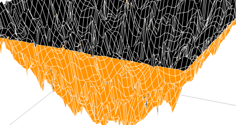
(b) Error after 6 unpreconditioned GMRES iterations

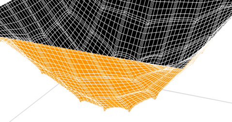
(c) Error after 6 Schwarz-smoothing iterations

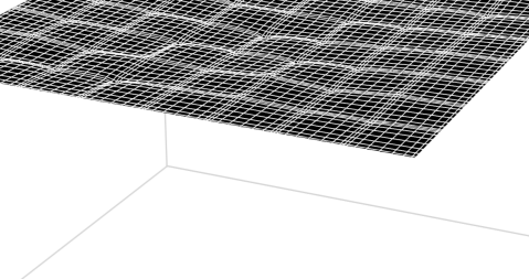
(d) Error after 1 multigrid-Schwarz V/̄cycle

Figure 11: Intermediate errors of the 2D sinusoidal Poisson problem (Sec. IV.1) with different components of the elliptic solver. Panel LABEL:sub@fig:poisson_smoothing_initial shows the error of the random initial guess. Panels LABEL:sub@fig:poisson_smoothing_noprec–LABEL:sub@fig:poisson_smoothing_mg show the error after six applications of the linear operator.

The following numerical tests demonstrate the accuracy, scalability, and parallel efficiency of the elliptic solver on a variety of linear and nonlinear elliptic problems.

All computations were performed on our local computing cluster Minerva. It is composed of 16-core nodes, each with two eight-core Intel Haswell E5-2630v3 processors clocked at $2.40\text{\,}\mathrm{GHz}$ and $64\text{\,}\mathrm{GB}$ of memory, connected with an Intel Omni-Path network. We distribute elements evenly among cores following the strategy detailed in Sec. III, leaving one core per node free to perform communications.

IV.1 A Poisson problem

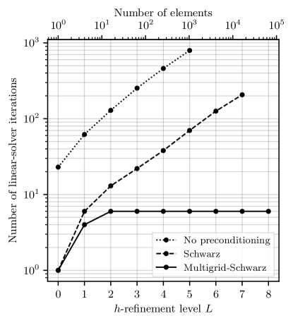
Figure 12: Number of linear-solver iterations for the Poisson problem (Sec. IV.1). The multigrid-Schwarz preconditioner achieves scale independence.

As a first test we solve the flat-space Poisson equation in two dimensions,

$$-\partial_{i}\partial_{i}u(\bm{x})=f(\bm{x})\text{,}$$ (34)

for the solution

$$u_{\text{analytic}}(\bm{x})=\sin{(\pi x)}\sin{(\pi y)}$$ (35)

on a rectilinear domain $\Omega=[0,1]^{2}$ with Dirichlet boundary conditions. This problem is also studied in the context of multigrid-Schwarz methods, with slight variations, in Refs. [53, 54]. To obtain the solution (35) numerically we choose the fixed source $f(\bm{x})=2\pi^{2}\sin{(\pi x)}\sin{(\pi y)}$, select homogeneous Dirichlet boundary conditions ${u^{\mathrm{b}}=0}$, and solve the DG-discretized problem (9) with penalty parameter ${C=1}$. We have evaluated the properties of the DG-discretized operator for this problem in Ref. [40]. To assess the convergence behavior of the elliptic solver for this test problem we choose an initial guess $\underline{u}_{0}$, where each value is uniformly sampled from $[-0.5,0.5]$.

Figure 11 illustrates the effectiveness of our algorithm in resolving small-scale and large-scale modes in the solution. Plotted is the error to the analytic solution, $\underline{u}-\underline{u}_{\mathrm{analytic}}$. Figure 11a depicts the initial error on a computational domain that is partitioned into $8\times 8$ quadratic elements with $9\times 9$ grid points each. Figures 11b to 11d present the error after six applications of the linear operator, but with different components of the elliptic solver enabled. Figure 11b employs no preconditioning at all, thus reaches six operator applications after six iterations of the GMRES algorithm. It resolves some of the random fluctuations, but retains the large-scale sinusoidal error. Figure 11c preconditions every GMRES iteration with six Schwarz-smoothing steps, thus reaches six operator applications after a single GMRES iteration. The Schwarz smoother uses $N_{\mathrm{overlap}}=2$. It resolves most of the random fluctuations, but retains the large-scale error. Note that the six operator applications do not accurately reflect the computational expense to arrive at Fig. 11c, because a significant amount of work is spent on the subdomain solves. We employ the explicit-inverse subdomain solver directly here to solve subdomain problems because the Laplacian-approximation preconditioner is redundant for a pure Poisson problem (see Sec. III.5), but note that the subdomain solver has no effect on the results depicted in Fig. 11 as long as it is sufficiently precise. Finally, Fig. 11d preconditions every GMRES iteration with a single four-level multigrid-Schwarz V/̄cycle. The V/̄cycle employs three Schwarz presmoothing and postsmoothing steps on every level, thus reaches six operator applications on the finest grid after a single GMRES iteration. Again, the number of operator applications is not entirely representative of the computational expense because it disregards the work done on coarser levels. The V/̄cycle successfully resolves the large-scale error.

Figure 12 presents the number of GMRES iterations that the elliptic solver needs to reduce the magnitude of the residual by a factor of $10^{10}$, for a series of $h$-refined domains. We construct $h$-refinement levels $L$ by repeatedly splitting all elements in the rectangular domain in two along both dimensions. All elements have $6\times 6$ grid points. Shown in Fig. 12 are an unpreconditioned GMRES algorithm, a GMRES algorithm preconditioned with three Schwarz-smoothing steps per iteration, and a GMRES algorithm preconditioned with one multigrid-Schwarz V/̄cycle per iteration. The number of multigrid levels is equal to the number $L$ of refinement levels, so that the coarsest level always covers the entire domain with a single element. Every level runs three presmoothing and postsmoothing steps, and subdomains have $N_{\mathrm{overlap}}=2$. The Schwarz preconditioning alone reduces the number of iterations by a factor of $\sim 10$, but does not affect the scaling with element size. However, the multigrid-Schwarz preconditioning removes the scaling entirely, meaning the number of GMRES iterations remains constant even when the domain is partitioned into more and smaller elements. The multigrid algorithm achieves this scale independence because it supports the iterative solve with information from coarser grids, including large-scale modes in the solution that span the entire domain. Each preconditioned iteration is typically more computationally expensive than an unpreconditioned iteration, but the preconditioner reduces the number of iterations such that the solve completes faster overall. We find that even for the simple Poisson problem the unpreconditioned algorithm becomes prohibitively slow around $\mathcal{O}(10^{3})$ elements ($L=5$), approaching an hour of runtime and the memory capacity of our ten compute nodes. In contrast, the Schwarz preconditioner reduces the runtime to solve the same problem to below one minute, and the multigrid-Schwarz preconditioner reduces the runtime to only three seconds. Crucial to achieving these runtimes at high resolution are the parallelization properties of the algorithms. In particular, the additional computational expense that the preconditioner spends Schwarz-smoothing all multigrid levels is parallelizable within each level. The following test problem IV.2 explores the parallelization in greater detail.

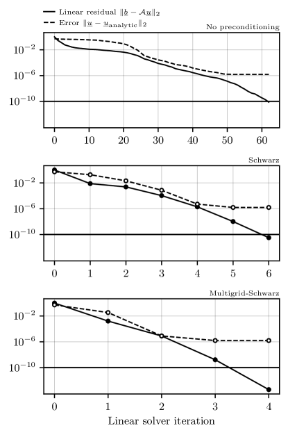
Figure 13: Convergence of the elliptic solver for the linear Poisson problem with $h$-refinement level $L=1$. The solid line shows the relative linear-solver residual magnitude $\lVert\underline{b}-\mathcal{A}\underline{u}\rVert_{2}$, and the dashed line shows the error to the analytic solution, $\lVert\underline{u}-\underline{u}_{\mathrm{analytic}}\rVert_{2}$ as a root mean square over grid points, which approaches the DG discretization error.

Figure 13 gives a detailed insight into the convergence behavior of the elliptic solver for the $L=1$ configuration. Presented is both the linear-solver residual magnitude $\lVert\underline{b}-\mathcal{A}\underline{u}\rVert_{2}$, and the error to the analytic solution, $\lVert\underline{u}-\underline{u}_{\mathrm{analytic}}\rVert_{2}$. The linear-solver residual (solid line) is being reduced by a factor of $10^{10}$ by the GMRES algorithm, equipped with the three different preconditioning configurations explored in Fig. 12. With no preconditioning, the convergence stagnates until large-scale modes in the solution are resolved (see also Fig. 11). The Schwarz preconditioner reduces the number of iterations by about an order of magnitude, and the multigrid-Schwarz preconditioner achieves clean exponential convergence. The error to the analytic solution (dashed line) follows the convergence of the residual magnitude. Once the discrete problem $\mathcal{A}\underline{u}=\underline{b}$, Eq. 1, is solved to sufficient precision, the remaining error $\underline{u}-\underline{u}_{\mathrm{analytic}}$ is the DG discretization error. It is independent of the computational technique used to solve the discrete problem, and determined entirely by the discretization scheme on the computational grid, as summarized in Sec. II and detailed in Ref. [40].

IV.2 A black hole in general relativity

Next, we solve a general-relativistic problem involving a black hole. Specifically, we solve the Einstein constraint equations in the XCTS formulation, Eq. 4, for a Schwarzschild black hole in Kerr-Schild coordinates. To this end we set the conformal metric and the trace of the extrinsic curvature to their respective Kerr-Schild quantities,

$$\bar{\gamma}_{ij} =\delta_{ij}+\frac{2M}{r}l_{i}l_{j}$$ (36a)

and

$$K =\frac{2M\alpha^{3}}{r^{2}}\left(1+\frac{3M}{r}\right)\text{,}$$ (36b)

where $M$ is the mass parameter, $r=\sqrt{x^{2}+y^{2}+z^{2}}$ is the Euclidean coordinate distance, and $l^{i}=l_{i}=x^{i}/r$. The time-derivative quantities $\bar{u}_{ij}$ and $\partial_{t}K$ in the XCTS equations (4) vanish, as do the matter sources $\rho$, $S$, and $S^{i}$. With these background quantities specified, the solution to the XCTS equations is

$$\psi =1\text{,}$$ (37a)

$$\alpha =\left(1+\frac{2M}{r}\right)^{-1/2}\text{,}$$ (37b)

$$\beta^{i} =\frac{2M}{r}\alpha^{2}l^{i}\text{.}$$ (37c)

Note that we have chosen a conformal decomposition with $\psi=1$ here, but other choices of $\psi$ and $\bar{\gamma}_{ij}$ that keep the spatial metric $\gamma_{ij}=\psi^{4}\bar{\gamma}_{ij}$ invariant are equally admissable.

We solve the XCTS equations numerically for the conformal factor $\psi$, the product $\alpha\psi$, and the shift $\beta^{i}$. The conformal metric $\bar{\gamma}_{ij}$ and the trace of the extrinsic curvature, $K$, are background quantities that remain fixed throughout the solve. Note that for this test problem the conformal metric $\bar{\gamma}_{ij}$ is not flat, resulting in a problem formulated on a curved manifold.

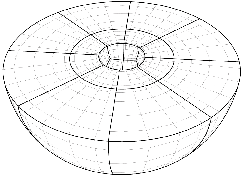
Figure 14: A cut through the uniformly-refined spherical-shell domain used in the black hole problem (Sec. IV.2). The domain consists of six wedges with a logarithmic radial coordinate map enveloping an excised sphere. In this example each wedge is isotropically $h$-refined once, i.e., split once in all three dimensions, resulting in a total of 48 elements. Note the elements are split in half along their logical axes, so the element size scales logarithmically in radial direction just like the distribution of grid points within the elements. Each element has six grid point per dimension, so fields are represented as polynomials of degree five.

We employ the DG scheme (9) with penalty parameter ${C=1}$ to discretize the XCTS equations (4) on a three-dimensional spherical-shell domain, as illustrated in Fig. 14. The domain envelops an excised sphere that represents the black hole, so it has an inner and an outer external boundary that require boundary conditions. To obtain the Schwarzschild solution in Kerr-Schild coordinates we impose Eqs. 37a to 37c as Dirichlet conditions at the outer boundary of the spherical shell at $r=10M$. We place the inner radius of the spherical shell at $r=2M$ and impose mixed Dirichlet and Neumann conditions at the inner boundary. Specifically, we impose the Neumann condition $n^{i}\partial_{i}\psi=0$ on the conformal factor, and Eqs. 37b to 37c as Dirichlet conditions on the lapse and shift. The reason for this choice is to mimic apparent-horizon boundary conditions, as employed in the following test problem (Sec. IV.3). Choosing apparent-horizon boundary conditions for the Kerr-Schild problem is also possible, but requires either an initial guess close to the solution to converge, or a conformal decomposition different from $\psi=1$. The reason is the strong nonlinearity in the apparent-horizon boundary conditions that takes the solution away from $\psi_{0}=1$ initially. We have confirmed this behavior of the XCTS equations with the SpEC code, and have presented the convergence of the DG discretization error with apparent-horizon boundary conditions for the Kerr-Schild problem in Ref. [40]. With the simpler Dirichlet and Neumann boundary condition we can seed the elliptic solver with a flat initial guess, i.e., $\psi_{0}=1$, $\alpha_{0}=1$ and $\beta_{0}^{i}=0$, which allows for better control of the test problem.

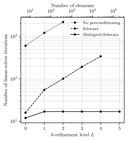
Figure 15: Number of linear-solver iterations for the black hole problem (Sec. IV.2). The multigrid-Schwarz preconditioner achieves scale independence. The $L=1$ configuration (48 elements) is pictured in Fig. 14.

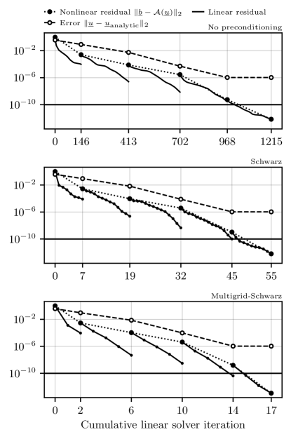
Figure 16: Convergence of the Newton-Krylov elliptic solver for the black hole problem with $h$-refinement level $L=1$. The dotted line shows the relative residual magnitude of the nonlinear solver, $\lVert\underline{b}-\mathcal{A}\underline{u}\rVert_{2}$, which is driven by a linear solve in every iteration (solid lines, see Eq. 16). The dashed line shows the error to the analytic solution, $\lVert\underline{u}-\underline{u}_{\mathrm{analytic}}\rVert_{2}$ as a root mean square over all five variables of the XCTS equations, $\{\psi,\alpha\psi,\beta^{i}\}$, and over grid points. It approaches the DG discretization error.

To assess the convergence behavior of the elliptic solver for this problem we successively $h$-refine the wedges of the spherical-shell domain into more and smaller elements, each with six grid points per dimension. We iterate the Newton-Raphson algorithm until the magnitude of the nonlinear residual has decreased by a factor of $10^{10}$. In all configurations we have tested, the nonlinear solver needs five steps and no line-search globalization to reach the target residual. The linear solver is configured to solve the linearized problem, Eq. 16, by reducing its residual magnitude by a factor of $10^{4}$. Schwarz subdomains have $N_{\mathrm{overlap}}=2$, and we run three Schwarz presmoothing and postsmoothing iterations on every multigrid level, including the coarsest. Figure 15 presents the total number of linear-solver iterations accumulated over the five nonlinear solver steps. Just like we found for the simple Poisson problem in Fig. 12, the multigrid-Schwarz preconditioner achieves scale-independent iteration counts under $h$ refinement.

Figure 16 presents the convergence behavior of the elliptic solver for the $L=1$ configuration (pictured in Fig. 14) in detail. The convergence of the nonlinear residual magnitude (dotted line) is independent of the preconditioner chosen for the linear solver in each iteration (solid lines), since the linearized problems are solved to sufficient accuracy ($10^{-4}$). Similar to the Poisson problem in Fig. 13, the multigrid-Schwarz preconditioning achieves clean exponential convergence, reducing the linear residual by an order of magnitude per iteration. The nonlinear residual magnitude decreases slowly at first, when the fields $\underline{u}$ are still far from the solution, and begins to converge quadratically, following the linear-solver residual, once the fields are closer to the solution and hence the linearization is more accurate (see Sec. III.1). The error to the analytic solution (dashed line) approaches the DG discretization error, as detailed in Sec. IV.1.

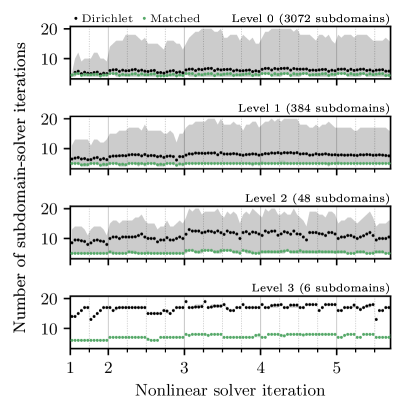
Figure 17: Number of subdomain-solver iterations for the black hole problem (Sec. IV.2) with the Laplacian-approximation preconditioner. The domain is isotropically $h$-refined thrice, so the solve involves four multigrid levels. Dots illustrate the average across all subdomains on the level, and shaded regions the smallest and largest number of iterations. When approximating all equations with a Dirichlet-Laplacian (black), subdomains facing the inner excision boundary (see Fig. 14) require more iterations than the average. Matching the Laplacian boundary conditions to the problem (green) reduces the iteration count and resolves the load imbalance.

To solve subdomain problems here we equip the GMRES subdomain solver with the Laplacian-approximation preconditioner, and solve the five Poisson subproblems on every subdomain with the incomplete LU explicit-inverse solver (see Sec. III.5). Figure 17 illustrates the importance of matching the boundary conditions of the approximate Laplacian to the original problem. When we approximate all five tensor components of the original XCTS problem with a Dirichlet-Laplacian, ignoring that we impose Neumann-type boundary condition on $\psi$ at the inner boundary, some subdomains require a significantly larger number of subdomain-solver iterations than others. We have confirmed that these subdomains face the inner boundary of the spherical shell. When we use a Laplacian approximation with matching boundary-condition type for these subdomains, they need no more subdomain-solver iterations than interior subdomains. Specifically, the subdomain preconditioner constructs a Poisson operator matrix with homogeneous Neumann boundary conditions to apply to the conformal-factor component of the equations, and another with homogeneous Dirichlet boundary conditions to apply to the remaining four tensor components. Therefore, subdomains that face the inner boundary of the spherical shell domain build and cache two inverse matrices, and all other subdomains build and cache a single inverse matrix, in the form of an incomplete LU decomposition. Furthermore, when the Laplacian-approximation preconditioner takes the type of boundary conditions into account, we find that it is sufficiently precise so we can limit the number of subdomain-solver iterations to a fixed number. This further balances the load between elements, decreasing runtime significantly in our tests. Therefore, in the following we always limit the number of subdomain-solver iterations to three. With this strategy we find a reduction in runtime of about $50\text{\,}\mathrm{\char 37\relax}$ compared to the naive Dirichlet-Laplacian approximation.

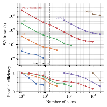
Figure 18: Parallel scaling of the black hole problem (Sec. IV.2).

Figure 18 presents the wall time and parallel efficiency of the elliptic solves for the black hole problem on up to 2048 cores, which approaches the capacity of our local computing cluster. We split the domain into more and smaller elements, keeping the number of grid points in each element constant at six per dimension, and solve each configuration on a variable number of cores. These configurations are increasingly expensive to solve, involving up to 42 million grid points, or $\sim 200$ million degrees of freedom. They all complete in at most a few minutes of wall time by scaling up to a few thousand cores, until they reach the capacity of our cluster. We compute their parallel efficiency as

$$\text{Parallel efficiency}=\frac{t_{\text{serial}}}{t_{\text{CPU}}}\text{,}$$ (38)

where $t_{\text{CPU}}=N_{\text{cores}}\,t_{\text{wall}}$ is the CPU time of a run, i.e., the product of wall time and the number of cores, and $t_{\text{serial}}$ is the wall time of the configuration runing on a single core. Since configurations with 24576 elements and more did not complete on a single core in the allotted time of two hours, we approximate $t_{\text{serial}}$ with the CPU time of the run with the lowest number of cores for these configurations, meaning that they begin at a fiducial parallel efficiency of one. The parallel efficiency decreases when the number of elements per core becomes small and falls below $25\text{\,}\mathrm{\char 37\relax}$ once each core holds only a few elements.

Figure 18 also shows that the parallel efficiency decreases more steeply when filling up a single node, than it does when we begin to allocate multiple nodes. We take this behavior as an indication that shared hardware resources on a node currently limit our parallel efficiency, which is an issue also found in Ref. [55]. We have confirmed this hypothesis by running a selection of configurations on the same number of cores, but distributed over more nodes, so each node is only partially subscribed, and found that runs speed up significantly. We intend to address this issue in future optimizations of the elliptic solver. Possible resolutions include better use of CPU caches, e.g., through a contiguous layout of data on subdomains, or a shared-memory OpenMP parallelization of subdomain solves, so the cores of a node are working on a smaller amount of data at any given time. The parallel efficiency also decreases once we reach the capacity of our cluster, at which point we expect that communications spanning the full cluster dominate the computational expense. We intend to test the parallel scaling on larger clusters with more cores per node in the future. We also plan to investigate the effect of hyperthreading on the parallel efficiency of the elliptic solver.

IV.3 A black hole binary

Finally, we solve a classic black hole binary (BBH) initial data problem, which stands at the beginning of every BBH simulation performed with the SpEC code. Again, we solve the full Einstein constraint system in the XCTS formulation, Eq. 4, but now we choose background quantities and boundary conditions that represent two black holes in orbit. Following the formalism for superposed Kerr-Schild initial data, e.g., laid out in Ref. [59, 60], we set the conformal metric and the trace of the extrinsic curvature to the superpositions

$$\bar{\gamma}_{ij} =\delta_{ij}+\sum_{n=1}^{2}e^{-r_{n}^{2}/w_{n}^{2}}\,(\gamma_{ij}^{(n)}-\delta_{ij})$$ (39a)

and

$$K =\sum_{n=1}^{2}e^{-r_{n}^{2}/w_{n}^{2}}K^{(n)}\text{,}$$ (39b)

where $\gamma_{ij}^{(n)}$ and $K^{(n)}$ are the conformal metric and extrinsic-curvature trace of two isolated Schwarzschild black holes in Kerr-Schild coordinates as given in Eq. 36. They have mass parameters $M_{n}$ and are centered at coordinates $\bm{C}_{n}$, with $r_{n}$ being the Euclidean coordinate distance from either center. The superpositions are modulated by two Gaussians with widths $w_{n}$. The time-derivative quantities $\bar{u}_{ij}$ and $\partial_{t}K$ in the XCTS equations (4) vanish, as do the matter sources $\rho$, $S$ and $S^{i}$.

To handle orbital motion we split the shift in a background and an excess contribution [14],

$$\beta^{i}=\beta^{i}_{\mathrm{background}}+\beta^{i}_{\mathrm{excess}}\text{,}$$ (40)

and choose the background shift

$$\beta^{i}_{\mathrm{background}}=(\bm{\Omega}_{0}\times\bm{x})^{i}\text{,}$$ (41)

where $\bm{\Omega}_{0}$ is the orbital angular velocity. We insert Eq. 40 in the XCTS equations (4) and henceforth solve them for $\beta^{i}_{\mathrm{excess}}$, instead of $\beta^{i}$.

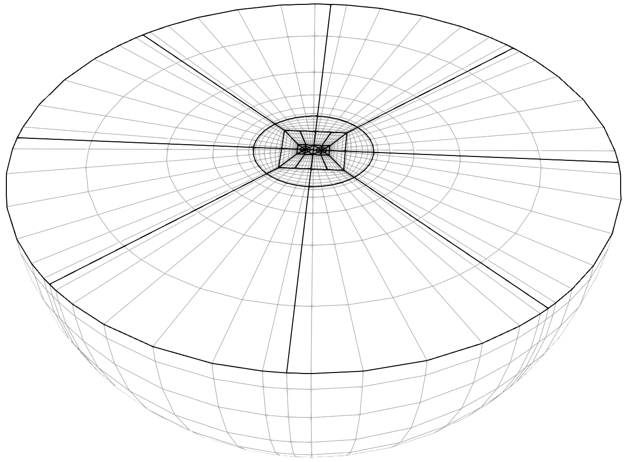
(a) Black hole binary domain

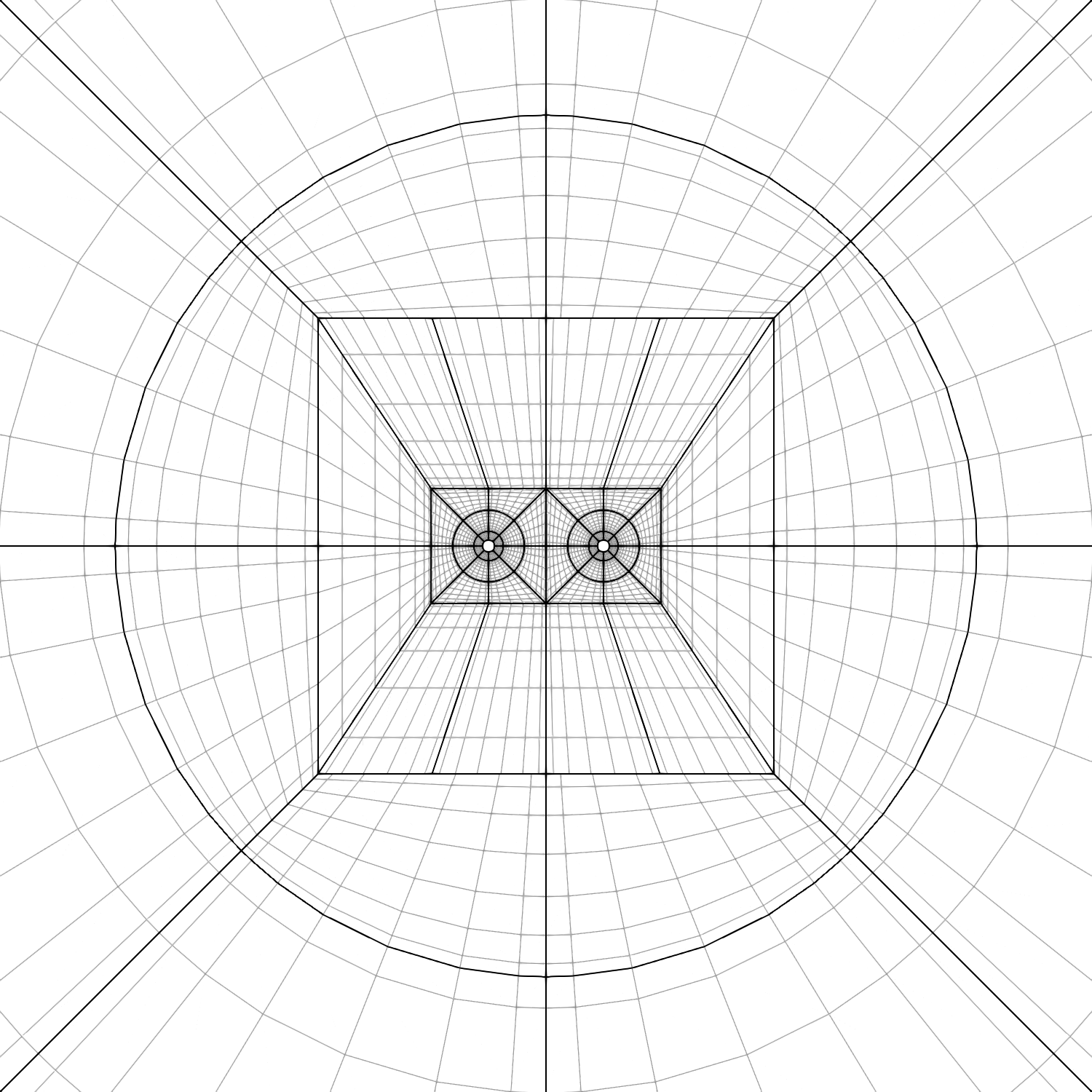
(b) Close-up

Figure 19: A cut through the three-dimensional black hole binary domain used in Sec. IV.3. It involves two excised spheres centered at $\bm{C}_{n}$ along the $x$-axis and extends to a spherical outer surface at radius $R$. The domain is $h$-refined such that spherical wedges have equal angular size, so the cube-to-sphere boundary is nonconforming. All elements in this picture have eight angular grid points, and $\{7,8,8,9,11,11\}$ radial grid points in the layers ordered from outermost to innermost.

We solve the XCTS equations on the domain depicted in Fig. 19. It has two excised spheres with radius $2M_{n}$ that are centered at $\bm{C}_{n}$, and correspond to the two black holes, and an outer spherical boundary at finite radius $R$. We impose boundary conditions on these three boundaries as follows. At the outer spherical boundary of the domain we impose asymptotic flatness,

$$\psi=1\text{,}\quad\alpha\psi=1\text{,}\quad\beta_{\mathrm{excess}}^{i}=0\text{.}$$ (42)

Since the outer boundary is at a finite radius, the solution will only be approximately asymptotically flat. On the two excision boundaries we impose (nonspinning) quasiequilibrium apparent-horizon boundary conditions [61]

$$\bar{s}^{k}\partial_{k}\psi={} -\frac{\psi^{3}}{8\alpha}\bar{s}_{i}\bar{s}_{j}\left((\bar{L}\beta)^{ij}-\bar{u}^{ij}\right)$$

$$-\frac{\psi}{4}\bar{m}^{ij}\bar{\nabla}_{i}\bar{s}_{j}+\frac{1}{6}K\psi^{3}\text{,}$$ (43a)

$$\beta^{i}={} \frac{\alpha}{\psi^{2}}\bar{s}^{i}\text{,}$$ (43b)

where $\bar{m}^{ij}=\bar{\gamma}^{ij}-\bar{s}^{i}\bar{s}^{j}$. Here, $\bar{s}_{i}=-n_{i}=\psi^{-2}s_{i}$ is the conformal surface normal to the apparent horizon, which is opposite the normal to the domain boundary since both are normalized with the conformal metric. For the lapse we choose to impose the isolated solution, Eq. 37b, as Dirichlet conditions at both excision surfaces. Note that this choice differs slightly from Ref. [60], where the superposed isolated solutions are imposed on the lapse at both excision surfaces.

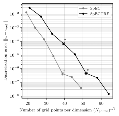
(a)

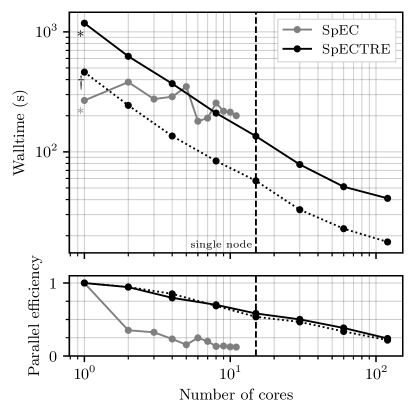
(b)

Figure 20: Comparison of the BBH initial data problem (Sec. IV.3) solved with our new elliptic solver in SpECTRE (black), and with the SpEC elliptic solver (gray). Left: Both codes converge exponentially with resolution. SpECTRE needs about $30\text{\,}\mathrm{\char 37\relax}$ more grid points per dimension than SpEC to reach the same accuracy. Right: Parallel scaling of both codes. The SpEC elliptic solver scales to at most eleven cores and reaches a speedup of at most a factor of two compared to the single-core runtime. Our new elliptic solver in SpECTRE is faster than SpEC on eight cores, and scales the problem reliably to 120 cores, at which point it is seven times faster than SpEC’s single-core runtime. The dotted line corresponds to a configuration with the same number of grid points as SpEC (but lower accuracy), which is faster than SpEC on only two cores.

To assess the accuracy and parallel performance of the elliptic solver for the BBH initial data problem we solve the same scenario with the SpEC [14, 19] code. In SpEC we successively increment the resolution from Lev0 to Lev6, which correspond to domain configurations determined with an adaptive mesh-refinement (AMR) algorithm. In SpECTRE we simply increment the number of grid points in all dimensions of all elements by one from each resolution to the next, based on the domain depicted in Fig. 19. To compare the solution between the two codes, we interpolate all five fields $u_{A}=\{\psi,\alpha\psi,\beta_{\mathrm{excess}}^{i}\}$ to a set of sample points $\bm{x}_{m}$. We do the same for a very high-resolution run with SpECTRE that we use as reference, $u_{A,\mathrm{ref}}$, for which we have split every element in the domain in two along all three dimensions. Then, we compute the discretization error for all SpEC and SpECTRE solutions as an $L_{2}$-norm of the difference to the high-resolution reference run over all fields and sample points,

$$\lVert u-u_{\mathrm{ref}}\rVert\coloneqq\left(\sum_{A,m}\left(u_{A}(\bm{x}_{m})-u_{A,\mathrm{ref}}(\bm{x}_{m})\right)^{2}\right)^{1/2}\mkern-22.0mu\text{.}$$ (44)

We have chosen $M_{n}=0.4229$, $\bm{C}_{n}=(\pm 8,0,0)$, $\Omega_{0}=0.0144$, $w_{n}=4.8$, $R=300$, and sample points along the $x$-axis at $x_{1}=8.846$ (near horizon), $x_{2}=0$ (origin) and $x_{3}=100$ (far field) here. This configuration coincides with our convergence study in Ref. [40], where we list the reference values $u_{A,\mathrm{ref}}(\bm{x}_{m})$ at the interpolation points explicitly.

Figure 20 compares the performance of the BBH initial data problem with the SpEC code. Both SpEC and SpECTRE converge exponentially with resolution, since SpEC employs a spectral scheme and SpECTRE a DG scheme under $p$ refinement. SpECTRE currently needs about $30\text{\,}\mathrm{\char 37\relax}$ more grid points per dimension to achieve the same accuracy as SpEC. To an extent this is to be expected, since we split the domain into more elements than SpEC does and hence have more shared element boundaries with duplicate points. In particular, SpEC employs shells with spherical basis functions that avoid duplicate points in angular directions altogether. While the SpEC elliptic solver always decomposes the domain into eleven subdomains, each with up to 34 grid points per dimension in our test, our domain in SpECTRE has 232 elements with up to 13 grid points per dimension. However, neither is our BBH domain in SpECTRE optimized as well as SpEC’s yet, nor have we refined it with an AMR algorithm. We are planning to do both in future work. Furthermore, SpEC’s initial data domain involves overlapping patches to enable matching conditions for its spectral scheme, which our DG scheme in SpECTRE does not need. Therefore, we expect to achieve domain configurations that come closer to SpEC in their number of grid points with future optimizations.

The right panel in Fig. 20 demonstrates the superior parallel performance that our new elliptic solver achieves over SpEC’s. We choose the runs marked with ^∗ in the left panel because they solve the BBH problem to comparable accuracy. We scale these runs to an increasing number of cores and measure the wall time for the elliptic solves to complete. Since the SpEC initial data domain is composed of eleven subdomains, it can parallelize to at most eleven cores. The runtime decreases by a factor of about 1.5 to 2 when the solve is distributed to multiple cores, but shows little reliable scaling. Some SpEC configurations at higher resolutions have shown slightly better parallel performance, but none that exceeded a factor of about two in speedup compared to the single-core runtime. Our new elliptic solver in SpECTRE, on the other hand, scales reliably to 120 cores, at which point each core holds no more than two elements. On a single core it needs $1176\text{\,}\mathrm{s}$ where SpEC, with fewer grid points, needs only $268\text{\,}\mathrm{s}$, but it overtakes SpEC on eight cores and completes in only $37\text{\,}\mathrm{s}$ on 120 cores. For reference we have also included a scaling test with SpECTRE that uses the same number of grid points as SpEC but does not yet reach the same accuracy (marked with ^†). It overtakes SpEC on two cores and completes in only $14\text{\,}\mathrm{s}$ on 120 cores. The configuration represents a potential improvement in the domain decomposition with future optimizations. We find the parallel efficiency for the BBH configurations behaves similarly to the single black hole configurations we investigated in Sec. IV.2.

V Conclusion and future work

We have presented a new solver for elliptic partial differential equations that is designed to parallelize on computing clusters. It is based on discontinuous Galerkin (DG) methods and task-based parallel iterative algorithms. We have shown that our solver is capable of parallelizing elliptic problems with $\sim 200$ million degrees of freedom to at least a few thousand cores. It solves a classic black hole binary (BBH) initial data problem faster than the veteran code SpEC [19] on only eight cores, and in a fraction of the time when distributed to more cores on a computing cluster. The elliptic solver is implemented in the open-source SpECTRE [29] numerical relativity code, and the results in this article are reproducible with the supplemental input-file configurations.

So far we can solve Poisson, elasticity, puncture and XCTS problems, including BBH initial data in the superposed Kerr-Schild formalism with unequal masses, spins and negative-expansion boundary conditions [60] (in this article we only explored an equal-mass and nonspinning BBH). In the short term we are planning to add the capability to solve for binary neutron star (BNS) and black hole–neutron star (BHNS) initial data, which involve the XCTS equations coupled to the equations of hydrostatic equilibrium.

A notable strength of our new elliptic solver is the multigrid-Schwarz preconditioner, which achieves iteration counts independent of the number of elements in the computational domain. Therefore, we expect our solver to scale to problems that benefit from $h$ refinement, e.g., to resolve different length scales or to adapt the domain to features in the solution. Such problems include initial data involving neutron stars with steep gradients near the surface, equations of state with phase transitions, or simulating thermal noise in thin mirror coatings for gravitational-wave detectors [62, 63].

Our solver splits the computational domain into more elements than the spectral code SpEC to achieve superior parallelization properties. However, the larger number of elements with shared boundaries also means that we need more grid points than SpEC to reach the same accuracy for a BBH initial data problem. Variations of the DG scheme, such as a hybridizable DG method, can provide a possible resolution to this effect [64, 65, 66]. Even without changing the DG scheme, we expect that optimizations of our binary compact object domain can significantly reduce the number of grid points required to reach a certain accuracy. Possible domain optimizations include combining the enveloping cube and the cube-to-sphere transition into a single layer of blocks, equalizing the angular size of the enveloping wedges in a manner similar to Ref. [24], or more drastic changes that involve cylindrical or bipolar coordinate maps, such as the domain presented in Ref. [67]. To retain the effectiveness of the multigrid solver it is important to keep the number of blocks in the domain to a minimum under these optimizations. We have shown that our new elliptic solver reaches comparative single-core performance to SpEC when using the same number of grid points, with the added benefit of parallel scaling. Since every contemporary computer has multiple cores, we prioritize parallelization over single-core performance.

To put the grid points of the computational domain to most effective use, adaptive mesh-refinement (AMR) techniques will be essential. All components of the elliptic solver, including the DG discretization, the multigrid algorithm, and the Schwarz subdomains, already support $hp$-refined domains. The refinement can be anisotropic, meaning elements can be split or differ in their polynomial degree along each dimension independently. A major subject of future work will be the development of an AMR scheme that adjusts the refinement during the elliptic solve automatically based on a local error estimate, distributing resolution to regions in the domain where it is most needed.

Along with AMR, we expect load balancing to become increasingly important. We currently approximately load balance the elliptic solver at the beginning of the program based on the number of grid points in each element. Charm++, and hence SpECTRE, also support dynamic load-balancing operations that migrate elements between cores periodically, or at specific points in the algorithm. Charm++ provides a variety of load-balancing algorithms that may take metrics such as runtime measurements, communication cost and the network topology into account. When the computational load on elements changes due to $p$-AMR, or when elements get created and destroyed due to $h$-AMR, we intend to invoke load balancing to improve the parallel performance of the elliptic solves.

The elliptic solver algorithms can be improved in many ways. The multigrid solver may benefit from an additive variant of the algorithm, which smooths every level independently and combines the solutions [55]. An additive multigrid algorithm has better parallelization properties than the multiplicative algorithm that we employ in this article, since coarse grids do not need to wait for fine grids to send data before the coarse-grid smoothing can proceed. However, the additive multigrid algorithm typically requires more iterations to converge than the multiplicative. Furthermore, multigrid patterns other than the standard V/̄cycle may accelerate convergence, such as a W/̄cycle or F/̄cycle pattern [51].

Schwarz solvers also come in many variations, e.g., involving face-centered subdomains, that we have not explored in this article. Our element-centered subdomains that eliminate corner and edge neighbors have served well for our DG-discretized problems so far, and we have focused on accelerating the subdomain solves with suitable preconditioners. Faster explicit-construction and approximate-inversion techniques for the subproblems in the Laplacian-approximation preconditioner have the greatest potential to speed up the elliptic solver. Possibilities include constructing matrix representations analytically, either from the DG scheme or from an approximate finite-difference scheme, and faster methods to solve the subproblems than the incomplete LU technique we currently employ.

A possible avenue for a more drastic improvement of the elliptic solver algorithm is to replace the multigrid-Schwarz preconditioner, or parts of it, altogether. For example, recent developments in the field of physics-informed neural networks (PINNs) suggest that hybrid strategies, combining a traditional linear solver with a PINN, can be very effective [68, 69]. Hence, an intriguing prospect for accelerating elliptic solves in numerical relativity is to combine our Newton-Krylov algorithm with a PINN preconditioner, use the PINN as a smoother on multigrids, or use it to precondition Schwarz subdomain solves.

Looking ahead, fast, scalable and highly-parallel elliptic solves in numerical relativity not only have the potential to accelerate initial data construction to seed high-resolution simulations of general-relativistic scenarios, and at extreme physical parameters, but they may also support evolutions. For example, some gauge constraints can be formulated as elliptic equations, and solving them alongside an evolution can allow the choice of beneficial coordinates, such as maximal slicing [1]. The apparent-horizon condition is also an elliptic equation, though current NR codes typically find apparent horizons with a parabolic relaxation method [70]. Some NR codes employ a constrained-evolution scheme, which evolves the system in time through a series of elliptic solves, or employ implicit-explicit (IMEX) evolution schemes [71]. Lastly, Einstein-Vlasov systems for collisionless matter involve elliptic equations, as do simulations that involve solving a Poisson equation alongside an evolution, such as simulations of self-gravitating protoplanetary disks [72, 73, 74]. Currently, elliptic solvers are rarely applied to solve any of these problems alongside an evolution because they are too costly. Fast elliptic solves have the potential to enable these applications.