Kinetic Event-Chain Algorithm for Active Matter

Abstract

We present a cluster kinetic Monte-Carlo algorithm for active matter systems of self-propelled hard particles. The kinetic event-chain algorithm is based on the event-chain Monte-Carlo method and is applied to active hard disks in two dimensions. The algorithm assigns Monte-Carlo moves of active disks a mean time based on their mean move length in force direction. This time is used to perform diffusional rotation of their propulsion force. We show that the algorithm reproduces the motility induced phase separated region in the phase diagram of hard disks correctly and efficiently. We extend the algorithm to mixtures of active and passive particles and uncover the microscopic mechanism behind the enhanced diffusion of a completely symmetric passive tracer disk in a bath of active hard disks.

Active matter systems are non-equilibrium many-particle systems which are driven by energy supplied by a propulsion force at the level of individual particles. Active matter can be found at all length scales and both for synthetic and biological systems [1]; examples comprise self-propelled colloidal particles [2] and microswimmers [3], cytoskeletal filaments propelled by molecular motors [4, 5, 6], colonies of bacteria [7], and swarms of animals [8].

In the simplest active systems, the propulsion force direction is anchored to the individual particle, which breaks the rotational symmetry at the particle level, and changes direction upon diffusive re-orientation of the particle. The propulsion energy sets particles in motion and is dissipated via a surrounding bath, which breaks detailed balance and gives rise to non-equilibrium physics. The most popular theoretical and numerical model are active Brownian particles (ABPs) with an overdamped motion and a heat bath modeled by Brownian random forces (Langevin dynamics).

Interacting active matter exhibits novel collective phenomena, which are not present in the corresponding equilibrium systems. One prominent example is the motility induced phase separation (MIPS) of self-propelled hard spheres [9, 10], which is an activity-driven clustering phenomenon driven by the active blocking of particles with opposing propulsion directions. More complicated phase behavior occurs for non-spherical particles or in the presence of alignment interactions [1].

Despite considerable progress during the last decade [11], simulation methods for active many-particle systems are largely limited to Langevin or molecular dynamics (MD) techniques. While MC algorithms produced much of the numerical progress in statistical physics of equilibrium phase transitions, the development of kinetic Monte-Carlo (kMC) schemes for active matter started only recently [12, 13, 14]. Moreover, cluster MC algorithms have not been proposed at all for active systems so far, while rejection-free cluster MC algorithms have proven to be a powerful tool for lattice spin systems [15, 16] and – as event-chain (EC) MC [17] – also for off-lattice simulations of many-particle systems.

In this paper, we present the first cluster kinetic Monte-Carlo scheme for the simulation of active matter systems of self-propelled hard particles. The algorithm is a kinetic event-chain (kEC) algorithm based on the ECMC method. The kEC algorithm is demonstrated for, but not limited to active hard disks in two dimensions. We verify and benchmark the novel kEC algorithm by calculating the phase diagram of active hard disks and mapping out the MIPS region.

We then go on to demonstrate the power of the new simulation method by addressing mixtures of active and passive particles or active suspensions containing passive tracers. It is long known that perfectly spherical passive tracers show enhanced persistent diffusion in an active bath [7, 18], but a microscopic explanation for this phenomenon is still elusive. Using the novel kEC algorithm, we reveal that this microscopic mechanism is based on a preferential clustering of propelling active particles at the rear side (aft) of a moving passive particle.

Kinetic event-chain Monte-Carlo algorithm.

EC algorithms are a variant of irreversible Markov-Chain MC algorithms [19] and have been applied to a wide range of systems in the last decade [17, 20, 21, 22, 23, 24, 25, 26]. They can also be classified as cluster algorithms. In a hard disk system, an EC cluster is constructed by choosing a random unit direction ${\bm{e}}_{\text{EC}}$ and a random initial disk. Starting with the initial disk, the “moving” disk is displaced in direction ${\bm{e}}_{\text{EC}}$ until collision with another disk. In a billiard-like fashion, the hit disk becomes the “moving” disk (in a so-called lifting move) and is displaced in direction ${\bm{e}}_{\text{EC}}$ up to the next collision. The EC ends if the total displacement equals a prescribed EC length $\ell_{\text{EC}}$, which is a parameter of the EC algorithm. The resulting cluster moves of chains of particles are rejection-free and satisfy global balance rather than detailed balance [17, 21]. Compared to local Metropolis-Hastings MC [27], speed-ups of up to two orders of magnitude can be achieved [17, 22, 25].

MC algorithms are not based on an equation of motion and, thus, lack a proper definition of time. ABPs, on the other hand, are described by Brownian dynamics. A system of $N$ active particles (particle index $i$) in two dimensions, which are driven with propulsion force $F_{0}$ in the unit directions ${\bm{e}}_{i}(t)=\left(\cos(\theta_{i}),\sin(\theta_{i})\right)$, is described by $\dot{{\bm{r}}}_{i}(t)=v_{0}{\bm{e}}_{i}(t)+{\bm{\xi_{i}}}(t)+{\bm{f_{i}}}(t)$, where ${\bm{r}}_{i}(t)$ are the particle positions. Here, $v_{0}=F_{0}/\Gamma$ is the driving velocity for a friction constant $\Gamma$, and ${\bm{\xi_{i}}}(t)$ a Gaussian thermal noise with zero mean and correlations $\langle{\bm{\xi_{i}}}(t){\bm{\xi}}_{j}^{T}(t^{\prime})\rangle=2D{\bm{1}}\delta_{ij}\delta(t-t^{\prime})$, where $D=k_{B}T/\Gamma$ is the translational diffusion constant. The remaining active particles exert interaction forces ${\bm{f_{i}}}={\bm{F}}_{i}/\Gamma$; we will focus on hard disks of diameter $\sigma$. The propulsion direction ${\bm{e}}_{i}(t)$ undergoes free rotational diffusion, i.e., $\langle\dot{\theta}_{i}(t)\dot{\theta}_{j}(t^{\prime})\rangle=2D_{r}\delta_{ij}\delta(t-t^{\prime})$.

Individual active particles perform persistent random walks with a persistence time $1/D_{r}$ because the propulsion force direction undergoes rotational diffusion. Equilibrium MC algorithms lack this persistent motion because of their Markovian nature. Two kMC schemes have been proposed for active particles [12, 13, 14], where a temporal correlation of MC particle moves has been introduced to establish persistence. In conjunction with Metropolis sampling of interactions, these kMC schemes show non-equilibrium phenomena like MIPS for repulsive active particles. A mapping to ABPs cannot be established, however.

Here, we choose a different strategy and view each active particle as particle under its individual constant force $F_{0}{\bm{e}}$ and, thus, in its individual constant linear potential for each ECMC move. We will assign to each ECMC move a mean time $\langle\Delta t_{\text{EC}}\rangle$ based on the mean move length in force direction, $\Delta r_{e}\equiv\langle\Delta{\bm{r}}_{\text{EC}}\cdot{\bm{e}}\rangle$, We can calculate $\Delta r_{e}$ for the ECMC algorithm analytically as a function of $\beta F_{0}\ell_{\text{EC}}$ ($\beta={1}/{k_{\text{B}}T}$). Then we identify $\langle\Delta t_{\text{EC}}\rangle=\Delta r_{e}/v_{0}$ because $\langle\Delta{\bm{r}}\cdot{\bm{e}}\rangle=v_{0}\langle\Delta t\rangle$ holds for ABPs exactly. This introduces an exact mean time into the kEC algorithm, which we take to pass for each ECMC move employing a dynamical mean-field assumption to map onto ABPs. Using the time $\langle\Delta t_{\text{EC}}\rangle$, we readjust the force direction according to rotational diffusion after each EC move.

For the calculation of $\Delta r_{e}$, it is sufficient to consider a single active particle under a constant force $F_{0}{\bm{e}}$ or in a corresponding linear potential $V({\bm{r}})$. In an external potential, the ECMC algorithm works as follows [20, 24, 26]: A random EC direction ${\bm{e}}_{\text{EC}}$ is chosen. If the move is energetically downhill ($\cos\phi\equiv{\bm{e}}_{\text{EC}}\cdot{\bm{e}}\geq 0$), the particle is displaced by the full EC length, $\Delta{\bm{r}}=\ell_{\text{EC}}{\bm{e}}_{\text{EC}}$. If the move is energetically uphill ($\cos\phi<0$), a “usable” energy $\Delta U>0$ is drawn from a Boltzmann distribution $p(\Delta U)\sim\exp(-\beta\Delta U)$, and a rejection distance $d_{\text{rej}}$ is determined from $\Delta U=-F_{0}d_{\text{rej}}\cos\phi$. If $d_{\text{rej}}\geq\ell_{\text{EC}}$, the particle is moved by the full EC length, $\Delta{\bm{r}}=\ell_{\text{EC}}{\bm{e}}_{\text{EC}}$. If $d_{\text{rej}}<\ell_{\text{EC}}$, the particle is only moved by $\Delta{\bm{r}}=d_{\text{rej}}{\bm{e}}_{\text{EC}}$, the EC direction is lifted ${\bm{e}}_{\text{EC}}\to{\bm{e}}_{\text{EC}}^{\prime}$ (by reflecting with respect to the equipotential surface, i.e., ${\bm{e}}_{\text{EC}}^{\prime}={\bm{e}}_{\text{EC}}-2\cos\phi{\bm{e}}$), and the particle is moved by the remaining EC length $\ell_{\text{EC}}-d_{\text{rej}}$ in the new downhill direction. In total, this results in $\Delta{\bm{r}}=d_{\text{rej}}{\bm{e}}_{\text{EC}}+(\ell_{\text{EC}}-d_{\text{rej}}){\bm{e}}_{\text{EC}}^{\prime}$. After this EC move, a new direction ${\bm{e}}_{\text{EC}}$ is chosen, and we start over. Averaging over all cases and all randomly chosen directions ${\bm{e}}_{\text{EC}}$ (angles $\phi$), we obtain $\langle\Delta{\bm{r}}_{\text{EC}}\cdot{\bm{e}}\rangle/\beta F_{0}\ell_{\text{EC}}^{2}=f(\beta F_{0}\ell_{\text{EC}})$ with a scaling function [28]

$$f(x)=\frac{2}{\pi}\frac{1}{x}-\frac{1}{x^{2}}\frac{1}{\pi}\int_{-\pi/2}^{\pi/2}d\phi(1-e^{-x\cos\phi}).$$ (1)

For the ECMC move mean time, we identify $\beta F_{0}=v_{0}/D$ and obtain $\langle\Delta t_{\text{EC}}\rangle=(\ell_{\text{EC}}^{2}/D)f(v_{0}\ell_{\text{EC}}/D)$ such that $\langle\Delta t_{\text{EC}}\rangle$ only depends on the active force $F_{0}$ and the EC length $\ell_{\text{EC}}$. In the simulation, after each ECMC move, a new force direction as given by the angle $\theta^{\prime}$ is drawn from the Gaussian distribution $\sim\exp(-(\theta^{\prime}-\theta)^{2}\langle\Delta t_{\text{EC}}\rangle D_{r}/2)$. For a single active particle, this is only a good approximation if $\langle\Delta t_{\text{EC}}\rangle D_{r}\ll 1$. In terms of the active particle persistence length $L_{p}=v_{0}/D_{r}$, this means $L_{p}\gg v_{0}\langle\Delta t_{\text{EC}}\rangle$. For the important limit of large forces ($v_{0}\gg\sqrt{DD_{r}}$), where $\langle\Delta t_{\text{EC}}\rangle\sim\ell_{\text{EC}}/v_{0}$, this leads to the intuitive condition $\ell_{\text{EC}}\ll L_{p}$ for the algorithm to remain correct for single active particles. This is confirmed by tests with simple settings such as for an active particle in a constant force field as in sedimentation [28].

In the many-particle system, we combine the ECMC procedure for one active particle with the hard disk collision ECMC rules outlined above. Then, we simulate a Hamiltonian ${\cal H}=\sum_{i}[-F_{0}{\bm{e}}_{i}\cdot{\bm{r}}_{i}+V_{i}(\{{\bm{r}}_{i}\})]$, where active forces enter as individual external linear potentials, with the usual ECMC scheme assuming fixed ${\bm{e}}_{i}$ during each EC move. This results in ECs with more than one participating particle until the displacements $\Delta d_{i}$ of particles $i$ participating in an EC sum up to the total EC length $\ell_{\text{EC}}$, i.e., $\sum_{i\in\text{EC}}\Delta d_{i}=\ell_{\text{EC}}$. Each particle $i$ moves under a driving force $F_{0}{\bm{e}}_{i}$. In order to assign a proper time to each moving particle $i$ in the EC, we distribute the mean time $\langle\Delta t_{\text{EC}}\rangle$ of a single particle EC move without collisions over all particles $i$ in the EC according to their displacements $\Delta d_{i}=|\Delta{\bm{r}}_{\text{EC,i}}|$. Because collisions are instantaneous, we assign times $\langle\Delta t_{\text{EC}}\rangle_{i}=({\Delta d_{i}}/{\ell_{\text{EC}}})\langle t_{\text{EC}}\rangle$ to each particle then. After each EC, the force directions of all participating particles $i$ are drawn from a Gaussian distribution $\sim\exp(-(\theta_{i}^{\prime}-\theta_{i})^{2}\langle\Delta t_{\text{EC}}\rangle_{i}D_{r}/2)$. This means each particle has its “own simulation time”. We confirmed that the resulting simulation time is, on average, equal for all particles [28]. For many particles, the validity of the algorithm is much wider, as it requires $\langle\Delta t_{\text{EC}}\rangle_{i}D_{r}\ll 1$, which is a weaker condition in many-particle active systems, because $\langle\Delta t_{\text{EC}}\rangle_{i}\ll\langle\Delta t_{\text{EC}}\rangle$. For large forces, we obtain the validity condition $\ell_{\text{mfp}}\ll L_{p}$, where $\ell_{\text{mfp}}~{}(\ll\ell_{\text{MC}})$ is the mean free path in an EC.

Motility Induced Phase Separation.

We verify the novel kEC cluster algorithm by calculating the MIPS region in the phase diagram of active hard disks. Among all the numerical studies of active particles, results for genuine hard spheres are actually very rare [29, 30]. As opposed to fore-based Langevin or MD techniques, the kEC algorithm is particularly suited to study hard particles.

A salient feature of active hard spheres is the occurrence of MIPS for large propulsion forces [9, 31, 10] as controlled by the dimensionless Péclet number ${\rm Pe}=v_{0}/(\sigma D_{r})=L_{p}/\sigma$ (with $D_{r}=3D/\sigma^{2}$ [30]). The phase diagram of hard disks as a function of packing fraction $\eta=N\pi(\sigma/2)^{2}/A$ in a square system of area $A$ and the Péclet number ${\rm Pe}$ and the extent of the MIPS region provide a very sensitive test of any simulation technique. The results in Fig. 1 show good agreement with the hard disk results of Ref. 30 from Langevin simulations. We can perform simulations of $N=19500$ particles using the kEC algorithm, which are particle numbers that are hard to reach with Langevin simulations. Starting from a homogeneous initial packing we detect whether MIPS occurs (yellow points in Fig. 1) and determine the corresponding local coexisting packing fractions $\eta$ (binodals, black lines). Blue points between the coexistence lines correspond to global packing fractions, where the homogeneous initial state is only metastable, such that the boundary between blue and yellow points represents the spinodal line [28].

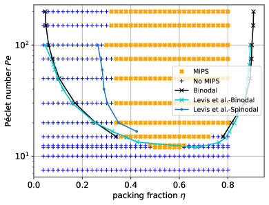
Figure 1: Phase diagram of active hard disks ($N=19500$ and $A$ changing according to packing fraction $\eta$) from kEC simulations [28]. The kEC results for binodal and spinodal agree with Langevin simulations results of Levis et al. [30].

Motion of passive tracers.

Finally, we apply the novel kEC algorithm to the important problem of a larger hard disk ($\sigma_{\text{large}}=20\sigma$ in Fig. 2) as completely symmetric passive tracer particle in a bath of smaller active hard disks. Mixtures of active and passive hard constituents can be easily implemented in kEC, where passive particles simply lack their individual propulsion force ($F_{0}=0$) but participate in kEC collisions. The motion of passive tracers in active systems gained wide attention in the field [7, 32, 18, 33, 34, 35, 36]. When the passive tracer particle has an anisotropic shape, symmetry is broken by shape, and various experiments and simulations confirm ballistic motion for short time scales [32, 33, 34, 33, 36]. It is long known that a very similar behaviour is observed in experiments with completely symmetric spherical tracers [7, 18], where the mechanism for the transient ballistic regime is still elusive.

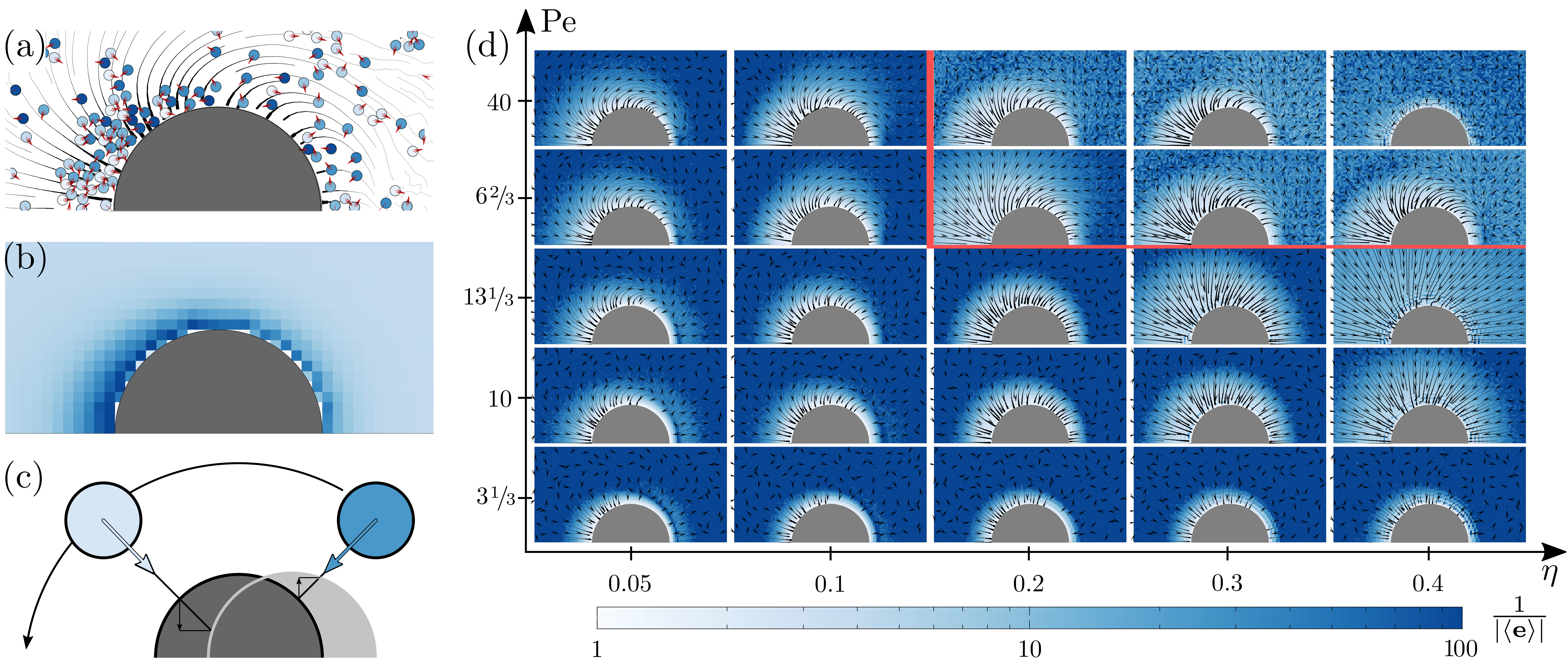
Figure 2: Simulation results in the eigenframe of the passive particle moving in positive x-direction. (a) Snapshot at $\eta=0.1$ and Pe$=26\nicefrac{{2}}{{3}}$, color codes for the angle of the active force which is also shown as vector. Streamlines of the average active force field show forces directed backwards. (b) Normalized density heat map in the eigenframe of the passive tracer particle. (c) Schematic of the proposed symmetry breaking mechanism. Active particles coming from the front (rear) collide at a higher (lower) y-position. This creates a higher density of wall-accumulated particles behind the passive tracer particle. (d) Spatially discretized mean active force $F_{0}\langle{\bm{e}}_{i}\rangle_{b}$ averaged over active particles in cells of size $b=0.5\sigma$ for different parameters in the $\eta$-${\rm Pe}$ phase plane. The arrows and streamlines indicate the direction $\langle{\bm{e}}_{i}\rangle_{b}$ of the mean active force field, color codes for $1/|\langle{\bm{e}}_{i}\rangle_{b}|$ such that deep blue corresponds to points with isotropic force distributions and white to anisotropic force distributions, where all active forces in a cell point in the same direction. The red line encompasses the systems exhibiting MIPS (see Fig. 1).

To characterize the motion of the passive tracer disk, we measure its mean-square displacement, its velocity, and the decorrelation of its displacement directions. We find a crossover from ballistic to diffusive motion at a characteristic time $\tau_{a}$ and an enhanced diffusivity with increasing packing fraction $\eta$ of active particles (outside the MIPS region and and sufficiently high $\rm Pe$), which is due to an increase of $\tau_{a}$ [28]. The tracer diffusion constant exceeds the single active diffusion constant providing evidence for a genuinely cooperative driving mechanism.

Results in Fig. 2 reveal the underlying microscopic mechanism. Here, it is crucial to switch to the eigenframe of the tracer, i.e., to its center of mass system, rotated such that the displacements from the last recorded position of the tracer aligns with the positive x-axis. The persistent motion stems from a short-lived cluster of active particles, that spontaneously forms on the rear side of a moving passive tracer particle, see Fig. 2 (a), and pushes the particle. The location of the cluster and, thus, the direction of motion is a soft mode and can rotate by fluctuations on time scales $\tau_{a}$ giving rise to the observed crossover. The mechanism for the formation of the pushing cluster is a combination of (i) wall accumulation [37] and (ii) preferential attachment of pushing particles to a moving obstacle [35].

Wall accumulation gives rise to a higher density of active particles at the surface of the tracer (see Fig. 2 (b) and supplemental density heat maps [28]. Moreover, forces become sorted by wall accumulation such that forces of accumulated particles point radially inward on average (see Fig. 2 (a)). Wall accumulation is, however, symmetric for a symmetric resting tracer. The mechanism behind symmetry breaking and preferential attachment of pushing particles at the rear side (aft) of a moving particle is shown in Fig. 2 (c), where we consider the fate of potentially accumulating particles with forces pointing radially inward. If the passive tracer moves (by a spontaneous fluctuation) in positive x-direction, particles coming from the front (rear) collide at a higher (lower) y-position [35]. Therefore, particles coming from the front either miss the tracer or their radially inward direction becomes redirected to the rear side. This gives rise to the characteristic distorted radial force streamline pattern around a moving tracer in Figs. 2 (a,d), which clearly shows that the preferred forces are no longer strictly radial but acquire a backward component. This mechanism maintains a higher active particle density on the rear side, which, in turn, stabilizes motion in x-direction.

Figure 2 (d) shows that the mechanism remains functional in the entire $\eta$-${\rm Pe}$ phase plane apart from the MIPS region. At the onset of MIPS, the picture changes and $\tau_{a}$ drops sharply. In the MIPS region, the passive sphere acts as a nucleation site for a high density phase cluster that surrounds the tracer completely. Then, there is a high uniform active density around the tracer and no symmetry breaking. As a results the passive particle slowly diffuses in the high density cluster until it eventually reaches its edge, where it is ejected into the dilute phase. This is supported by density heat maps [28], which show a small packing fraction around a passive tracer in the MIPS region. It follows that there is a maximal motility enhancement at parameters close to but not within the MIPS phase region, which is confirmed by Fig. 2.

Discussion.

We introduced a kinetic cluster MC algorithm for active systems, the kinetic event-chain (kEC) algorithm. The basic idea is to assign a mean time $\langle\Delta t_{\text{EC}}\rangle_{i}$ to all particle moves participating in a cluster EC move under the action of the active forces and to use this mean time to rotate active forces diffusively after each cluster move. This establishes a mapping onto ABPs. Our simulations of active hard disks show that the algorithm is correct and performant and can open the way for a more effective simulation of other active systems.

We can justify the algorithm rigorously for hard active particles, which are always force-free until collisions occur. Future efforts should aim to generalize the algorithm to soft interactions, such as Lennard-Jones interactions. We conjecture that our algorithm will produce accurate results with $\langle\Delta t_{\text{EC}}\rangle_{i}$ calculated based on the propulsion force $F_{0}$ only, as long as interaction forces can be neglected until particles come very close, such that an instantaneous collision picture remains valid. For a single sedimenting active particle in a constant force field ${\bm{F}}_{g}$, we find that we have to use the total force $|F_{0}{\bm{e}}+{\bm{F}}_{g}|$ instead of $F_{0}$ in the calculation of $\langle\Delta t_{\text{EC}}\rangle$ to get the correct sedimentation profiles [28]. A generalization to interacting particles could involve to calculate a mean interaction force along each EC cluster move, which is used in calculating its mean simulation time.

An additional advantage of the algorithm is that it can be easily extended to mixtures of active and passive hard particles. To show its capabilities, we investigated the motion of a large passive tracer disk in a bath of active hard disks and could solve the long-standing problem of the microscopic mechanism behind the enhanced diffusion and the existence of an initial ballistic regime [7].

I Supplemental Material

In this Supplementary Information, we present (i) details of the kEC algorithm, (ii) additional results for a sedimenting active particle, (iii) details of the kEC simulations for the phase diagram of hard disks, and (iv) supporting results on passive tracer motion in an active disk bath.

I.1 Details of the kEC algorithm

I.1.1 The algorithm

The kEC algorithm is based on the ECMC algorithm for hard spheres. Through factorization of the Metropolis filter each interaction can be handled entirely independently and sets a unique rejection distance $d_{\text{rej}}$. Roughly speaking, each interaction draws an Boltzmann distributed energy it can use until it would reject, which sets $d_{\text{rej}}$ for each interaction. After all interactions are evaluated, the shortest distance $d_{\text{rej}}$ is moved and the EC is lifted to the corresponding interaction partner, while the EC move direction ${\bm{e}}_{\text{EC}}$ remains. An EC is terminated when the sum of all displacements reach a pre-set length $\ell_{\text{EC}}$. In the presence of active forces, the corresponding linear one-particle potentials can also trigger rejection, which results in lifting of the EC direction to its reflection with respect to the equipotential surface (${\bm{e}}_{\text{EC}}^{\prime}={\bm{e}}_{\text{EC}}-2\mathbf{e}_{i}(\mathbf{e}_{i}\cdot{\bm{e}}_{\text{EC}})$), while the moving particle remains the same.

In a more structured way, an EC for active disks of diameters $\sigma_{i}$ is constructed as follows:

• Choose random particle $i$ and direction ${\bm{e}}_{\text{EC}}$ ($\lvert{\bm{e}}_{\text{EC}}\rvert=1)$ and determine $d_{\text{rej}}$, next active particle $i_{\text{next}}$ and eventually new EC-direction ${\bm{e}}_{\text{EC,next}}$

• Initial values
        $d_{\text{rej}}=\ell_{\text{EC}}$
        $i_{\text{next}}=i$
        ${\bm{e}}_{\text{EC,next}}={\bm{e}}_{\text{EC}}$

• Hard Spheres:
  for each particle $j\neq i$
        $\mathbf{R}=\mathbf{r}_{j}-\mathbf{r}_{i}$

        $\sigma_{ij}=0.5(\sigma_{i}+\sigma_{j})$

        $x=\mathbf{R}\cdot{\bm{e}}_{\text{EC}}$

        if $x>0$ (particles approach each other)

           $y=\sigma_{ij}^{2}-\mathbf{R}^{2}+x^{2}$

           if $y>0$ (particles can hit each other)
                 $d_{\text{rej},ij}=x-\sqrt{y}$

                 if $d_{\text{rej},ij}<d_{\text{rej}}$ (event before current one)

                    $d_{\text{rej}}=d_{\text{rej},ij}$

                    $i_{\text{next}}=j$

                    ${\bm{e}}_{\text{EC,next}}={\bm{e}}_{\text{EC}}$

• Active Force (if $F_{0,i}\neq 0$):

  $x=F_{0,i}(\mathbf{e}_{i}\cdot{\bm{e}}_{\text{EC}})$

  if $x<0$ (particle moves against the force)

        $y=\text{rand}[0\ldots 1]$

        $d_{\text{rej},\text{active}}={\text{ln}y}/{\beta x}$

        if $d_{\text{rej},\text{active}}<d_{\text{rej}}$ (event before current one)

           $d_{\text{rej}}=d_{\text{rej},\text{active}}$

           $i_{\text{next}}=i$

           ${\bm{e}}_{\text{EC,next}}={\bm{e}}_{\text{EC}}-2\mathbf{e}_{i}(\mathbf{e}_{i}\cdot{\bm{e}}_{\text{EC}})$

• Execute:

        $\mathbf{r}_{i}\mathrel{+}=d_{\text{rej}}{\bm{e}}_{\text{EC}}$

        $d_{i}\mathrel{+}=d_{\text{rej}}$

        $\ell_{\text{EC}}=\ell_{\text{EC}}-d_{\text{rej}}$

        $i=i_{\text{next}}$

        ${\bm{e}}_{\text{EC}}={\bm{e}}_{\text{EC,next}}$

• repeat until $\ell_{\text{EC}}=0$

• Rotate active forces:

  for each particle $i$

        $\langle\Delta t_{EC}\rangle_{i}=d_{i}\ell_{EC}f(v_{0}\ell_{EC}/D)$

        $\theta_{i}\mathrel{+}=\text{ Gauss}(0,\sqrt{2D_{r}\langle t_{EC}\rangle_{i}})$

        $d_{i}=0$

• Loop back to beginning

Here rand is a uniformly distributed and Gauss is a Gaussian distributed random number.

Typical parameters for two-dimensional hard disk systems that were used to determine the phase diagram in Fig. 1 in the main text and Fig. 6 are $N=19500$ simulated hard disks with EC length $\ell_{\text{EC}}=\sigma$. To give a rough idea of the performance of the algorithm, we measure the wall time for $Pe=50$, $\eta=0.12$ and $L=200$ (i.e., $N\approx 5000$) and get $3.6$ steps per second (Intel®Core^TM i7-8650U). A step consists of $10$ ECs with $\ell_{\text{EC}}=1\sigma$ started at each particle on average; measurements are conducted between each step.

I.1.2 Mean ECMC move time $\langle\Delta t_{\text{EC}}\rangle$

For the calculation of the mean move length in force direction, $\Delta r_{e}\equiv\langle\Delta{\bm{r}}_{\text{EC}}\cdot{\bm{e}}\rangle$, we consider a single particle under a constant force $F_{0}{\bm{e}}$. The ECMC algorithm draws a random direction ${\bm{e}}_{\text{EC}}$ and moves the particle by the EC length $\ell_{\text{EC}}$. We introduce the angle $\phi$ between the unit vectors ${\bm{e}}$ and ${\bm{e}}_{\text{EC}}$ by $\cos\phi\equiv{\bm{e}}_{EC}\cdot{\bm{e}}\geq 0$; the quantity $\Delta r_{e}$ is averaged over all angles $\phi$. Three cases have to be considered in the calculation of $\Delta r_{e}$ depending on $\phi$ and $\ell_{\text{EC}}$, and we have to properly average over these cases and all angles $\phi$.

(i) If $\cos\phi\geq 0$, the move is energetically downhill. Then the particle is displaced by the full EC length $\ell_{\text{EC}}$ resulting in a mean vectorial displacement

$$\langle\Delta{\bm{r}}_{\text{EC}}\rangle_{\cos\phi\geq 0}=\ell_{\text{EC}}{\bm{e}}_{EC}$$ (2)

for given $\phi$. Averaging over the all angles $\phi\in[-\pi/2,\pi/2]$ with $\cos\phi\geq 0$, we obtain

$$\langle\Delta{\bm{r}}_{\text{EC}}\cdot{\bm{e}}\rangle_{\geq} =\frac{1}{\pi}\int_{-\pi/2}^{\pi/2}d\phi\langle\Delta{\bm{r}}_{\text{EC}}\rangle_{\cos\phi\geq 0}\cdot{\bm{e}}$$

$$=\frac{1}{\pi}\ell_{\text{EC}}\int_{-\pi/2}^{\pi/2}d\phi\cos\phi=\frac{2}{\pi}\ell_{\text{EC}}$$ (3)

(ii) If $\cos\phi<0$, the move is energetically uphill. and a “usable” energy $\Delta U>0$ for uphill motion is drawn from an exponential Boltzmann distribution $p(\Delta U)\sim\exp(-\beta\Delta U)$ ($\beta=\frac{1}{k_{\text{B}}T}$) and a rejection distance $d_{\text{rej}}$ is determined from $\Delta U=F_{0}d_{\text{rej}}|\cos\phi|$. This is equivalent to drawing the rejection distance from an exponential distribution

$$p_{d}(d_{\text{rej}})=\beta F_{0}|\cos\phi|e^{-\beta F_{0}d_{\text{rej}}|\cos\phi|}.$$ (4)

Now, two subcases arise:

• $d_{\text{rej}}\geq\ell_{\text{EC}}$, where the particle is moved by the full event chain length, $\Delta{\bm{r}}=\ell_{\text{EC}}{\bm{e}}_{\text{EC}}$. This happens with probability

  $$p_{>}=\int_{\ell_{\text{EC}}}^{\infty}dxp_{d}(x)=e^{-\beta F_{0}\ell_{\text{EC}}|\cos\phi|}.$$ (5)

• $d_{\text{rej}}<\ell_{\text{EC}}$, where the particle is only moved by $\Delta{\bm{r}}=d_{\text{rej}}{\bm{e}}_{\text{EC}}$. Then, the EC direction is lifted ${\bm{e}}_{\text{EC}}\to{\bm{e}}_{\text{EC}}^{\prime}$ by reflecting with respect to the equipotential surface, ${\bm{e}}_{\text{EC}}^{\prime}={\bm{e}}_{\text{EC}}-2\cos\phi{\bm{e}}$. In total, this results in $\Delta{\bm{r}}=d_{\text{rej}}{\bm{e}}_{\text{EC}}+(\ell_{\text{EC}}-d_{\text{rej}}){\bm{e}}_{\text{EC}}^{\prime}$. This displacement is realized with probability $p_{d}(d_{\text{rej}})$.

Averaging over $p_{d}(d_{\text{rej}})$ we obtain for the mean vectorial displacement

$$\langle\Delta{\bm{r}}_{\text{EC}}\rangle_{\cos\phi<0}$$

$$=p_{>}\ell_{\text{EC}}{\bm{e}}_{EC}+\int_{0}^{\ell_{\text{EC}}}dxp_{d}(x)\left[x{\bm{e}}_{\text{EC}}+(\ell_{\text{EC}}-x){\bm{e}}_{\text{EC}}^{\prime}\right]$$

$$=p_{>}\ell_{\text{EC}}{\bm{e}}_{EC}$$

$$~{}~{}+\int_{0}^{\ell_{\text{EC}}}dxp_{d}(x)\left[\ell_{\text{EC}}{\bm{e}}_{\text{EC}}-2\cos\phi(\ell_{\text{EC}}-x){\bm{e}}\right]$$

$$=\ell_{\text{EC}}{\bm{e}}_{EC}$$

$$~{}~{}-2\cos\phi{\bm{e}}\int_{0}^{\ell_{\text{EC}}}dxp_{d}(x)(\ell_{\text{EC}}-x)$$

$$=\ell_{\text{EC}}{\bm{e}}_{EC}$$

$$~{}~{}-{\bm{e}}\frac{2}{\beta F_{0}}\left(1-\beta F_{0}\ell_{\text{EC}}|\cos\phi|-e^{-\beta F_{0}\ell_{\text{EC}}|\cos\phi|}\right)$$ (6)

for given $\phi$. Averaging over the all angles $\phi\in[\pi/2,3\pi/2]$ with $\cos\phi<0$, we obtain

$$\langle\Delta{\bm{r}}_{\text{EC}}\cdot{\bm{e}}\rangle_{\cos\phi<0}$$

$$=-\frac{1}{\pi}\int_{-\pi/2}^{\pi/2}d\phi\ell_{\text{EC}}\cos\phi$$

$$~{}~{}-\frac{2}{\beta F_{0}}\frac{1}{\pi}\int_{-\pi/2}^{\pi/2}d\phi\left(1-\beta F_{0}\ell_{\text{EC}}\cos\phi-e^{-\beta F_{0}\ell_{\text{EC}}\cos\phi}\right)$$

$$=\frac{2}{\pi}\ell_{\text{EC}}-\frac{2}{\beta F_{0}}\frac{1}{\pi}\int_{-\pi/2}^{\pi/2}d\phi\left(1-e^{-\beta F_{0}\ell_{\text{EC}}\cos\phi}\right)$$ (7)

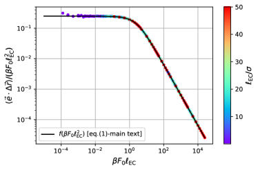
Figure 3: Mean ECMC move lengths in force direction $\langle\Delta{\bm{r}}_{\text{EC}}\cdot{\bm{e}}\rangle$ in units of $\beta F_{0}\ell_{\text{EC}}^{2}$ as a function of $x=\beta F_{0}\ell_{\text{EC}}$. The simulation data for difference $\ell_{\text{EC}}$ (color-coded) collapse onto the scaling function $f(x)$ from eq. (1) in the main text.

Averaging over the two cases $\cos\phi\geq 0$ and $\cos\phi<0$, we finally obtain

$$\Delta r_{e} =\frac{1}{2}\left(\langle\Delta{\bm{r}}_{\text{EC}}\cdot{\bm{e}}\rangle_{\geq}+\langle\Delta{\bm{r}}_{\text{EC}}\cdot{\bm{e}}\rangle_{<}\right)$$

$$=\frac{2}{\pi}\ell_{\text{EC}}-\frac{1}{\beta F_{0}}\frac{1}{\pi}\int_{-\pi/2}^{\pi/2}d\phi\left(1-e^{-\beta F_{0}\ell_{\text{EC}}\cos\phi}\right)$$

$$\frac{\Delta r_{e}}{\beta F_{0}\ell_{\text{EC}}^{2}} =\frac{2}{\pi}\frac{1}{\beta F_{0}\ell_{\text{EC}}}$$

$$~{}~{}-\frac{1}{(\beta F_{0}\ell_{\text{EC}})^{2}}\frac{1}{\pi}\int_{-\pi/2}^{\pi/2}d\phi\left(1-e^{-\beta F_{0}\ell_{\text{EC}}\cos\phi}\right)$$

$$=f(\beta F_{0}\ell_{\text{EC}})$$ (8)

with $f(x)$ from eq. (1) in the main text. The function $f(x)$ has the limiting behaviors $f(x)\approx 1/4-2x/9\pi$ for $x\ll 1$ (small forces $\beta F_{0}\ell_{\text{EC}}\ll 1$) and $f(x)\approx 2/\pi x-1/x^{2}$ for $x\gg 1$ (large forces $\beta F_{0}\ell_{\text{EC}}\gg 1$). Figure 3 shows perfect agreement of eq. (1) in the main text with the ECMC simulation.

In practice, the following fit function for $f(x)$ is useful:

$$f(x)=\frac{1}{ax+b\sqrt{x}+c}$$ (9)

with $a=\pi/2$, $b=-0.42$, and $c=4$, which is constructed to satisfy the limits $f(x)\approx 1/4$ for $x\approx 0$ and $f(x)\approx 2/\pi x$ for $x\to\infty$, so that $b$ is the only free parameter. The relative deviation from the exact result (1) in the main text is $<2\%$ (not visible on the scale of Fig. 3), so that this approximation can be used in production runs to speed up calculations.

I.2 Sedimenting active particle

We can perform ECMC simulations in the presence of an additional constant force ${\bm{F}}_{g}$ corresponding to an external potential $V({\bm{r}})=-{\bm{r}}\cdot{\bm{F}}_{g}$, for example, a gravitational force in sedimentation.

For a single particle in two dimensions, the stationary height distribution is exactly known to be exponential $p_{g}(y)=p_{0}\exp(-\lambda y)$ for ${\bm{F}}_{g}=-\Gamma v_{g}{\bm{y}}$. In the limit $v_{0}\gg v_{g}$, the sedimentation length becomes [38]

$$\lambda\approx\frac{2D_{r}v_{g}}{v_{0}^{2}}\left(1+\frac{7v_{g}^{2}}{4v_{0}^{2}}\right)~{}~{}~{}(v_{0}\gg v_{g}).$$ (10)

In the thermal limit $v_{0}\ll\sqrt{DD_{r}}$, we obtain the thermal (passive) sedimentation length $\lambda\approx\Gamma v_{g}/k_{B}T=v_{g}/D$.

We calculate the time $\langle\Delta t_{\text{EC}}\rangle$ using the total force ${\bm{F}}=F_{0}{\bm{e}}+{\bm{F}}_{g}$ for the data shown in Fig. 4. Then, Fig. 4 (a) shows that the kEC simulation results approach Brownian dynamics results for sufficiently small EC lengths $\ell_{\text{EC}}$. The condition of sufficiently small is discussed in the main text. According to this discussion, the kEC algorithm should be valid for $\ell_{\text{EC}}\ll L_{p}=v_{0}/D_{r}$ or $v_{0}/\sqrt{DD_{r}}\gg(\ell_{\text{EC}}/\sigma)\sqrt{\sigma^{2}D_{r}/D}$ in the limit of large forces. Thus, for increasing $\ell_{\text{EC}}$, the kEC algorithm becomes valid at increasingly large driving forces, which is confirmed in Fig. 4 (a).

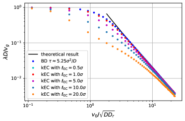
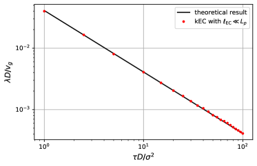
Figure 4: (a) Double logarithmic plot of dimensionless sedimentation length $\lambda D/v_{g}$ as a function of $v_{0}/\sqrt{DD_{r}}$ from Brownian dynamics (blue points) and kEC simulations with different EC lengths $\ell_{\text{EC}}$. Simulations are for $D_{r}\simeq 0.2D/\sigma^{2}$ and $v_{g}=0.2D/\sigma$. The theoretical result (10) is shown as black line. The results confirm that the kEC algorithm is only valid for $v_{0}/\sqrt{DD_{r}}\gg 0.45(\ell_{\text{EC}}/\sigma)$. (b) Double logarithmic plot of dimensionless sedimentation length $\lambda D/v_{g}$ as a function of $D/D_{r}\sigma^{2}$ for $v_{0}\sigma/D=7$ and $v_{g}=0.2D/\sigma$ using sufficiently short EC length $\ell_{\text{EC}}\ll L_{p}$. The theoretical result (10) is shown as black line.

Fig. 4 (b) demonstrates perfect agreement with the theoretical prediction eq. (10) for sufficiently short EC length $\ell_{\text{EC}}\ll L_{p}$. This demonstrates that the time $\langle\Delta t_{\text{EC}}\rangle$ should be calculated using the total force $|F_{0}{\bm{e}}+{\bm{F}}_{g}|$. Calculating the time $\langle\Delta t_{\text{EC}}\rangle$ using $F_{0}$ gives significantly worse results (not shown).

I.3 Details of the kEC simulations for the phase diagram of hard disks

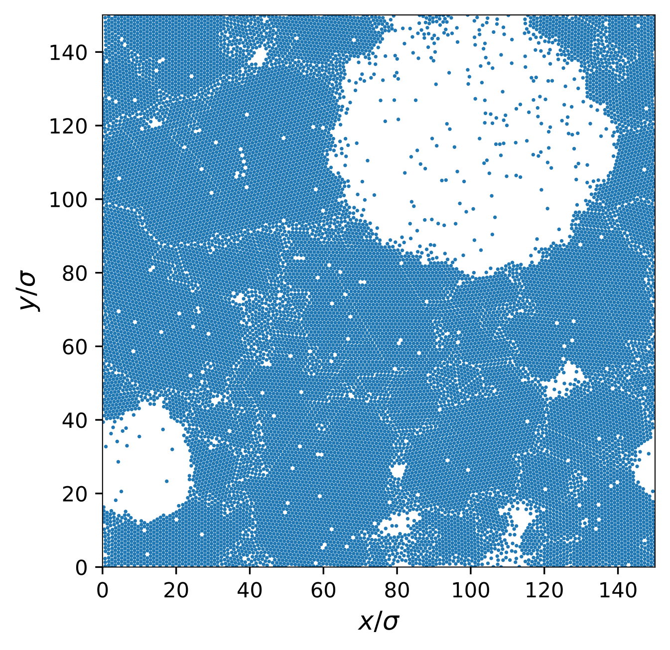
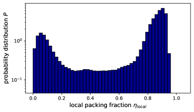
Figure 5: (a) Snapshot of a system exhibiting MIPS at ${\rm Pe}=75$ and $\eta=0.68$ ($N=19500$, $\ell_{\text{EC}}=\sigma$). (b) Corresponding histogram of local packing fractions $\eta_{\text{local}}$ using cells of area $A_{h}=(6\sigma)^{2}$.

In the kEC simulations we simulate $N=19500$ particles are almost homogeneously distributed in a square box with area $A=L^{2}$ and periodic boundary conditions. The initial state is an almost homogeneous distribution and the kEC algorithm is run with an EC length $\ell_{\text{EC}}=1.0\sigma$. For the simulations leading to the phase diagram in Fig. 1 in the main text, we change the global packing fraction $\eta=N\pi(\sigma/2)^{2}/A$ by changing the system size $L$ at fixed particle number $N=19500$. Depending on the Péclet number ${\rm Pe}=v_{0}/(\sigma D_{r})=L_{p}/\sigma$ (with $D_{r}=3D/\sigma^{2}$) and the global packing density, the phase behavior is classified and coexisting densities are determined.

From the densities coexisting for different global packing densities at the same Péclet number, the coexisting local packing fractions for this Péclet number (binodal points) are determined by averaging. The binodal points for different ${\rm Pe}$ give the phase coexistence lines (black lines in Fig. 1 in the main text).

The coexisting local packing fractions are determined from histograms of local packing fractions $\eta_{\text{local}}$, which are determined by counting disks in small square cells of area $A_{h}=(6\sigma)^{2}$, see example in Fig. 5. Maxima in the histogram are detected by comparison with 2 neighbors on each side and give the coexisting packing fractions of the phase diagrams in Fig. 1 in the main text.

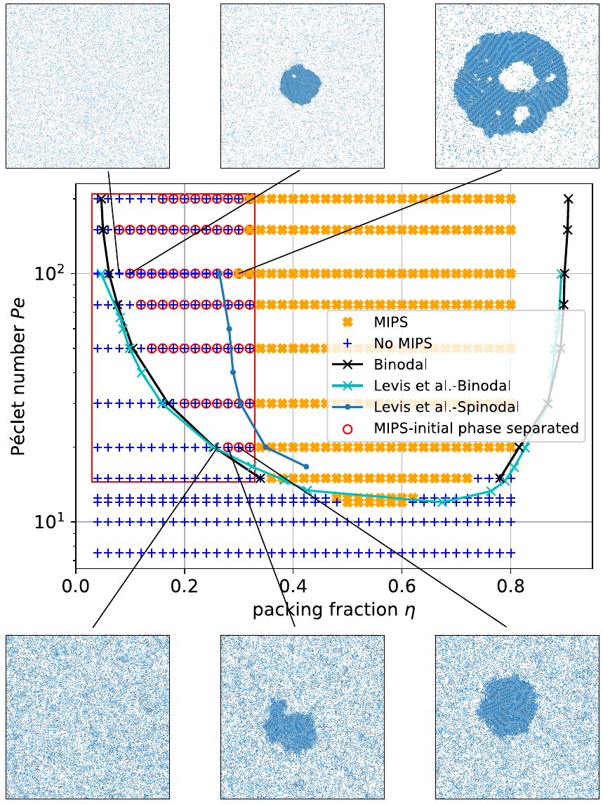
Figure 6: Results of additional simulations with phase separated initial state in the phase region enclosed by the red rectangle. The red circles are simulations with final states that show MIPS as indicated for some examples in the insets. This confirms that the boundary between blue and yellow points represents a spinodal line.

Blue points in Fig. 1 in the main text which lie between the coexistence lines correspond to global packing fractions, where the homogeneous initial state is only metastable. They should become unstable to MIPS by strong perturbations such as strong density fluctuations. To check this, some systems are simulated with $\eta\leq 0.32$, similar to Ref.  30, with an already phase-separated initial state, which we prepared by placing a dense and approximately square-shaped particle cluster in the center of the system. In addition, all driving forces are aligned in the direction of the system center initially. The results are shown in Fig. 6, where red circles represent systems with phase separated final states (see insets). We find that the phase separated state is a globally stable, while the homogeneous state only metastable, for practically all blue points which lie between the coexistence lines. Small deviations are due to finite-size effects. Especially near the binodal, systems separate into two phases such, that the dilute phase packing fraction approximately equals the global packing density.

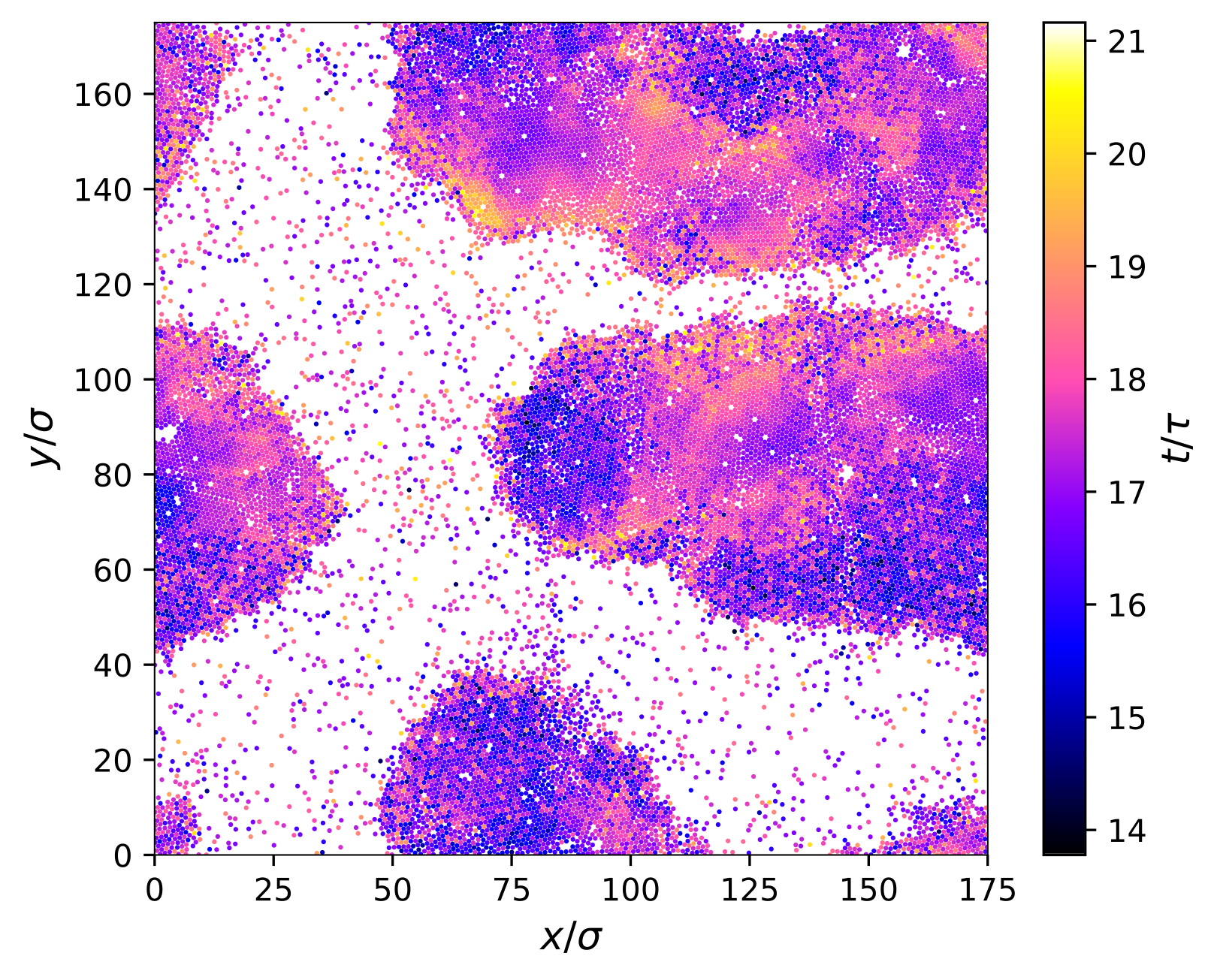
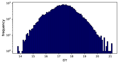
Figure 7: (a) Snapshot of a system exhibiting MIPS at ${\rm Pe}=225$ and $\eta=0.50$ ($N=19500$, $\ell_{\text{EC}}=\sigma$) with particles color coded for their “simulation time” as calculated from assigning to each EC move a time $\langle\Delta t_{\text{EC}}\rangle$, and to each particle a time $\langle\Delta t_{\text{EC}}\rangle_{i}=({\Delta d_{i}}/{\ell_{\text{EC}}})\langle t_{\text{EC}}\rangle$ (see main text). (b) Corresponding histogram of the simulation times of particles which is approximately Gaussian with a small relative standard deviation $\sigma/\mu=0.90/17.31=5.2\%$.

Each particle has its “own simulation time” in the kEC algorithm. In Fig. 7, we confirm that the resulting simulation time is, on average, equal for all particles for the active disk system. We choose a very heterogeneous system deep in the MIPS region (${\rm Pe}=225$ and $\eta=0.50$), but still observe a very narrow Gaussian distribution of particle simulation times with a relative standard deviation of only $5.2\%$.

I.4 Supporting results on passive tracer motion in an active disk bath

I.4.1 Enhanced persistent diffusion of passive tracer disk

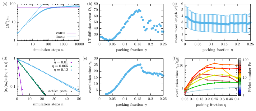
Figure 8: (a): Rescaled mean-squared displacements per simulation step as a function of simulations steps $n$ (in one simulation step $10$ ECs with $\ell_{\text{EC}}=1\sigma$ are started at each particle on average), for $Pe=50$ and $\eta=0.14$ showing an initial ballistic and asymptotic diffusive regime. (b): Long-term diffusion constants (constant fit over $n\in[100\ldots 1000]$) versus packing fraction $\eta$. At $\eta>\eta_{c}\approx 0.065$, the pushing becomes cooperative, and the tracer walk shows enhanced diffusion. (c): Mean move length per fixed measurement interval, which is proportional to the velocity of the tracer $v_{a}$. (d): Orientational decorrelation of the tracer for $Pe=50$ and three different packing fractions $\eta$. The orientational decorrelation for the smaller active disks is shown as black crosses. For $\eta>\eta_{c}$ and below the MIPS regime, the decorrelation time is enhanced. (e) Decorrelation time $\tau_{a}$ (measured in simulation steps) from exponential fits for $Pe=50$. At $\eta\approx 0.15$, MIPS occurs and the tracer effectively only sees the dilute phase. (f): Ratio of decorrelation times $\tau_{a}/\tau_{\text{act}}$ of the passive tracer and an active disk for different Péclet numbers (color coded, lines are for Péclet numbers $3\nicefrac{{1}}{{3}}$, $6\nicefrac{{2}}{{3}}$, $10$, $13\nicefrac{{1}}{{3}}$, ${20}$, $26\nicefrac{{2}}{{3}}$ ${40}$, ${53\nicefrac{{1}}{{3}}}$). At higher pushing forces and denser systems, the decorrelation times decrease due to the onset of MIPS.

To characterize the diffusive motion of the passive tracer disk, we measure its mean-square displacement (Fig. 8 (a,b)), its velocity (Fig. 8 (c)), and the decorrelation of its displacement directions (Fig. 8 (d,e,f)).

We choose active hard disks with ${\rm Pe}=50$, which roughly corresponds to E. coli or other active particles used in Refs. 7, 18, and study the influence of an active bath of increasing packing fraction $\eta$ on the diffusive properties of the passive tracer (in experiments in Refs. 7, 18 $\eta$ remains small enough to avoid MIPS).

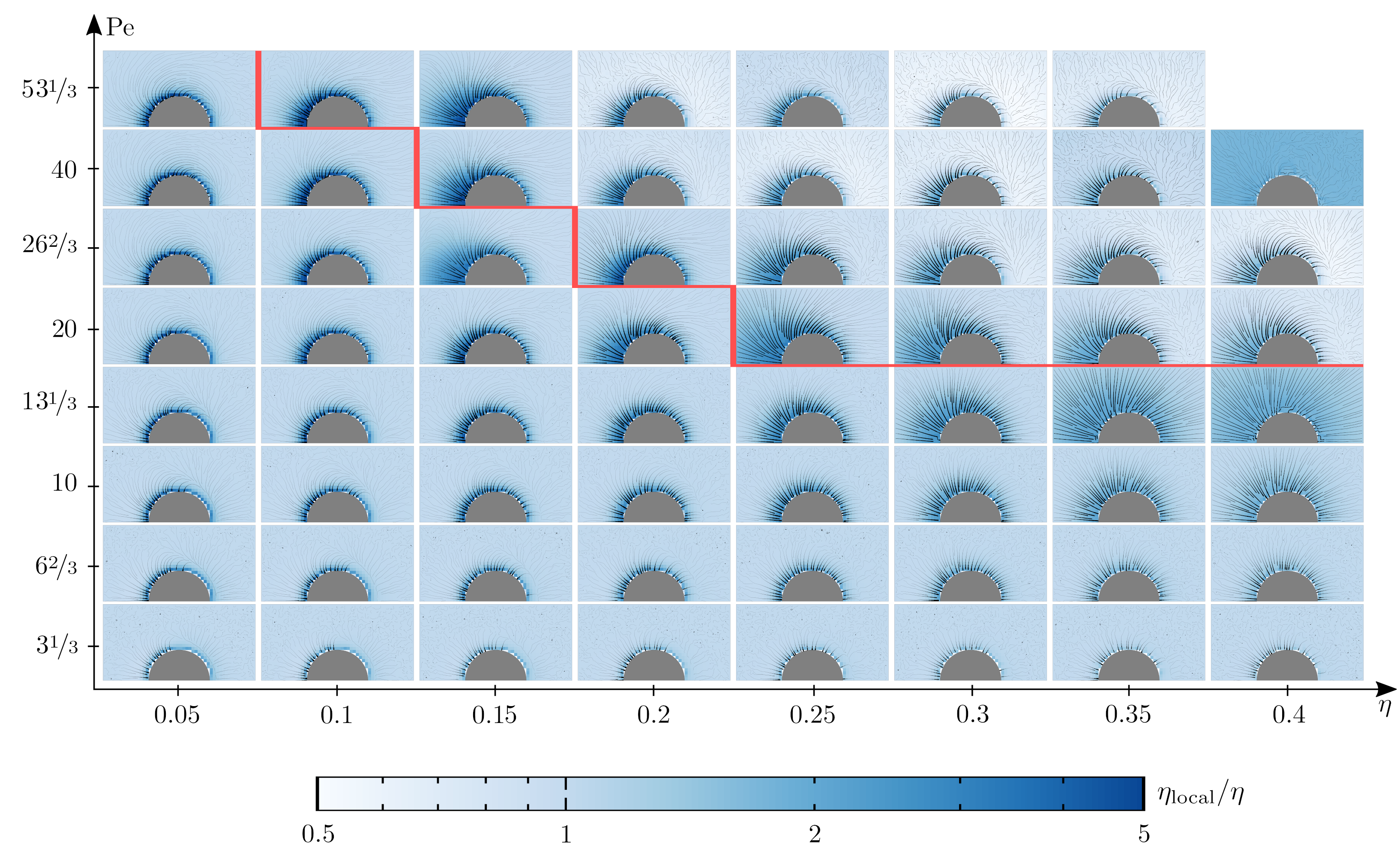
Figure 9: Normalized mean local packing fractions $\eta_{\text{local}}/\eta$ in the eigenframe of the passive tracer particle and streamlines of the average active force field for different parameters in the $\eta$-${\rm Pe}$ phase plane. The red line encompasses systems showing MIPS. Near the phase boundary, the symmetry breaking effect is most prominent. When active clusters occur in the MIPS phase region, the tracer is expelled into the dilute phase with a smaller local density $\eta_{\text{local}}/\eta<1$.

The mean-square displacement per step $\langle R^{2}\rangle/n$ in Fig. 8 (a) clearly shows that the passive tracer diffuses ($\langle R^{2}\rangle/n\sim{\rm const}$) asymptotically after many steps, but moves ballistically ($\langle R^{2}\rangle/n\sim n$) initially. Here, $n$ is the number of simulation steps. One simulation step corresponds to starting $10N$ ECs with $\ell_{\text{EC}}=1\sigma$, i.e., $10$ ECs at each particle on average. The crossover step size corresponds to the decorrelation time $\tau_{a}$ (also measured in simulation steps). The resulting diffusion constant $D_{a}=\langle R^{2}\rangle/n$ (measured in units of $\sigma^{2}$ per simulation step) increases for $\eta>\eta_{c}\approx 0.065$. At the critical value $\eta_{c}$, the pushing by active particles becomes cooperative, diffusion becomes enhanced, and increases linearly with $\eta$. The tracer walk actually has a higher diffusion constant than single active particles, which clearly shows the cooperativity of the driving mechanism. Around $\eta\approx 0.15$, MIPS sets in. Then the tracer is expelled into the dilute phase with a much smaller $\eta$, resulting in a reduced diffusion (the dilute phase at $Pe=50$ has $\eta\sim 0.1$ and the correlation time $\tau_{a}$ in the MIPS regime roughly corresponds to this packing fraction).

The mean velocity $v_{a}$ of the passive tracer is characterized via its mean move length per simulation step in Fig. 8 (c) and shows little variation as a function of $\eta$. Initially, the move length decreases as the mean free path shortens due to increasing density, but above $\eta_{c}$, the cooperative driving mechanism explained in the main text gives rise to a constant velocity.

The decorrelation of displacement directions is shown in Fig. 8 (d) in a log-linear plot. It clearly decays exponentially as a function of the number of simulation steps, $\langle{\bm{e}}_{a}(n_{0})\cdot{\bm{e}}_{a}(n_{0}+n)\rangle\sim\exp(-n/\tau_{a})$. Since each particle has its own local time, which increases linearly with its displacement, the number of ECs in a simulation step is chosen to be proportional to the number of particles in the system. This way, the number of steps and the mean global time are proportional to each other, if $F_{0}$ and $\ell_{\text{EC}}$ are kept constant. Therefore, the decay is also exponential in global time. For $\eta>\eta_{c}\approx 0.065$, the decorrelation time $\tau_{a}$ exceeds the decorrelation time of single active particles (black crosses), which clearly shows the cooperativity of the driving mechanism.

The correlation time $\tau_{a}$ increases with $\eta$ initially as shown in Fig. 8 (e), before it drops in the MIPS regime $\eta>0.15$. This shows that the enhanced diffusivity is a result of enhanced orientational correlations rather than an enhance mean velocity $v_{a}$.

Figure 8 (f) shows the ratio of decorrelation times $\tau_{a}/\tau_{\text{act}}$ of passive tracer and active disks (measured in the same system) as a function of the Péclet number $\rm Pe$ (color coded). All values $\tau_{a}/\tau_{\text{act}}>1$ indicate a cooperative driving mechanism. For small $\eta$, diffusion is enhanced by an increase in the decorrelation time $\tau_{a}$ before it decreases in the MIPS regime. For larger Péclet numbers $\rm Pe$, MIPS sets in at smaller $\eta$ according to the phase diagram Fig. 1 in the main text. The ratio $\tau_{a}/\tau_{\text{act}}$ depends non-monotonically on the Péclet number. These results also confirm that the maximal motility enhancement of the trace happens at parameters close to but not within the MIPS phase region (compare maximum of yellow and orange lines in Fig. 8 (f) and Fig. 2 in the main text).

I.4.2 Additional results on microscopic mechanism

Figure 9 complements Fig. 2 (d) in the main text and shows the normalized local packing fractions of active particles in the eigenframe of the passive tracer particle for different parameters in the $\eta$-${\rm Pe}$ phase plane, while Fig. 2 (d) showed the mean active force $F_{0}\langle{\bm{e}}_{i}\rangle_{b}$. Symmetry breaking gives rise to an increased density of propelling active particles at the rear side (aft) surface of the passive tracer.

The onset of MIPS is clearly visible in the simulations and is marked by a red line in both Figures. In the densest and most active system ($\eta=0.4$, Pe$=40$), the tracer particle is first nucleating and then trapped inside a MIPS cluster for the whole simulation time, indicated by the surrounding density in Fig.  9, which is higher than the mean density in the system. In the adjacent systems the tracer is expelled after a short time. Rather interesting is the system ($\eta=0.4$, Pe$=13\nicefrac{{1}}{{3}}$) close to the critical point in the isotropic phase. Here, the tracer repeatedly seeds clusters which vanish after short time. For more active systems, the clusters remains stable and for the more dilute and passive systems, clusters are unstable such that they are only observable in the direct vicinity of the passive tracer.

We want to note that very dilute systems ($\eta=0.05$) show a kind of bow wave, where forces away from the tracer seem preferable, but cannot offer a complete explanation for this phenomenon. Probably, a similar sorting mechanism as it is responsible for the rear cluster formation (as explained in the main text) could be the cause and should be investigated in the future.