One model Packs Thousands of Items with Recurrent Conditional Query Learning

Abstract

Recent studies have revealed that neural combinatorial optimization (NCO) has advantages over conventional algorithms in many combinatorial optimization problems such as routing, but it is less efficient for more complicated optimization tasks such as packing which involves mutually conditioned action spaces. In this paper, we propose a Recurrent Conditional Query Learning (RCQL) method to solve both 2D and 3D packing problems. We first embed states by a recurrent encoder, and then adopt attention with conditional queries from previous actions. The conditional query mechanism fills the information gap between learning steps, which shapes the problem as a Markov decision process. Benefiting from the recurrence, a single RCQL model is capable of handling different sizes of packing problems. Experiment results show that RCQL can effectively learn strong heuristics for offline and online strip packing problems (SPPs), outperforming a wide range of baselines in space utilization ratio. RCQL reduces the average bin gap ratio by 1.83% in offline 2D 40-box cases and 7.84% in 3D cases compared with state-of-the-art methods. Meanwhile, our method also achieves 5.64% higher space utilization ratio for SPPs with 1000 items than the state of the art.

Keywords Deep reinforcement learning  $\cdot$ Neural combinatorial optimization  $\cdot$ Packing problem

1 Introduction

How to pack boxes into the smallest bin? The answer to this deceivingly simple question is actually one of the most crucial ones that power today’s e-commerce. Zillions of boxes are being dispatched to customers each day from suppliers far and near. Being able to efficiently pack boxes compactly into bins and containers translates directly into reduced shipping costs and energy.

Packing problems, which are a type of classical combinatorial optimization problem (COP), have been extensively studied for many decades (Christensen et al., 2017) by researchers in operational research as well as those in computer science. Such a problem is strongly NP-hard (Martello et al., 2000) even when only one bin is considered, which is called the strip packing problem (SPP). Each packing step involves three interrelated actions, namely, item selection, rotation and positioning; what makes the problem acutely difficult is that later actions could be strongly affected by the previous actions. Therefore, exact algorithms (Silva et al., 2019) to achieve the optimal solution expectedly require a huge amount of computation time, and so they are only suitable for small-scale problems.

Other than exact algorithms, there are approximation and heuristic methods which tend to run faster. Some approximation algorithms (Christensen et al., 2017) provide solutions with a lower bound in polynomial time. Unfortunately, the results of these algorithms turned out to be not even as good as some simple packing algorithms (Crainic et al., 2008). Heuristic approaches (Baltacioglu et al., 2006; Gonçalves and Resende, 2011; Egeblad and Pisinger, 2009; Duong, 2015) define some rules based on human experience and knowledge about the problem. Some recent works (Wei et al., 2012, 2017) tried to improve on previous proposed heuristics by adding more rules; these methods however require substantial prior knowledge of the problem and thus lack flexibility in terms of the problem setting. Meta-heuristics (Rakotonirainy and van Vuuren, 2020; Zeng et al., 2016; Mostaghimi Ghomi et al., 2017; Wu et al., 2010) apply search methods to try to find better solutions in an iterative manner, but such a process takes a very long time at arrive at a good solution.

In fact, the explicit or hand-crafted rules of any special setting of a problem can be interpreted as policies in making decisions. Moreover, policies can be modeled by neural networks (NNs) in reinforcement learning. Hence, many recent studies (Bello et al., 2016; Nazari et al., 2018; Lu et al., 2019) have adopted NNs and reinforcement learning to solve classic COPs including the Traveling Salesman Problem (TSP), the Vehicle Routing Problem (VRP), etc. There were also some learning-based attempts (Duan et al., 2019; Cai et al., 2019) which utilize reinforcement learning with neural network models to solve packing problems.

However, these existing approaches either pay no attention to the connection between interrelated actions or they rely on hand-crafted rules in the learning algorithm. Without exploiting the connection between interrelated actions, the reinforcement learning environment becomes a partially observable Markov Decision Process (MDP) (Sutton and Barto, 2018) which is hard to generalize as a good policy due to lack of information. Those methods that use hand-crafted rules are not only unlikely to achieve an optimal solution, but are also overly sensitive to problem settings. Besides their relatively poor performance, previous learning based approaches also suffer from upsurge of memory costs as the number of boxes to be packed increases. These methods simply take all previously-packed boxes and the current candidate box states to infer the next packing actions, so the memory overhead increases rapidly as the problem size grows. Even worse, these models have to be re-trained for problems with different sizes because the model structure is problem size-related, thus posing a great challenge for practical applications.

In order to overcome the problems with previous learning methods, we introduce an end-to-end learning method called Recurrent Conditional Query Learning (RCQL) that directly addresses the information gap between interrelated actions. With the inner conditional query mechanism, the learning process is similar to a fully observable MDP, which makes training by reinforcement learning much easier. Compared with models that output several interrelated actions simultaneously where the action set per step is formed as a Cartesian product of the sub-action spaces, the action space of the RCQL model in each forward step equals the corresponding sub-action space. Such smaller action space allows us to apply a simpler model to fit the learning policy, which makes the model easier to train and more memory-efficient. Unlike previous learning-based approaches (Duan et al., 2019), RCQL does not involve any hand-craft rules or heuristics, and the whole model are trained by gradient-based learning method, making it an end-to-end learning method.

More specifically, the packing problem requires three mutually conditioned sub-actions: box selection, rotation and positioning. To fill the gap between sub-actions, we adopt the RCQL model as follows. First of all, the packing problem is formulated as an MDP for applying reinforcement learning. Then the previous sub-actions are embedded as a attention in the next sub-action decoder. After all three sub-actions have been generated, a packing step is performed and the observations are updated. Finally, we adopt the entropy regularized actor-critic algorithm (Haarnoja et al., 2018) to update the model parameters. In addition, because unpacked boxes and packed boxes have different properties, the input state of RCQL model is divided into two substates, which ensures that the model has a targeted representation of each substate. Furthermore, in order to deal with the sparse reward problem (Andrychowicz et al., 2017) in the packing problem, we design a novel gap-reward function, which entices the learning to converge faster.

Apart from the conditional query mechanism, the RCQL model also incorporates some recurrent attention features. That is, the model not only acquires information from the current environment state, but also gets information via an attention mechanism from previous hidden states to infer the subsequent step actions. In order to make recurrent attention work, the dynamic state updating is devised. Combining dynamic state updating and recurrence, the recurrence attention model enables learning dependency beyond current inputs without disrupting temporal coherence. This ensures that a fixed-size model can solve problems of different sizes without undermining the performance. At the same time, the model is suitable for on-line packing problems that are generally too hard for conventional algorithms.

We conduct extensive experiments to evaluate different models and the results show that the RCQL model achieves a lower gap ratio in both 2D and 3D packing than heuristic methods and existing learning approaches. Specifically, our model improves the space utilization ratio in 3D packing (40 boxes) by 29.32% compared with genetic algorithms, and reduces the bin gap ratio in almost every case by more than 7% compared with the state-of-the-art learning approaches. Furthermore, RCQL can scale to handle even thousands of boxes with only 2.16M model parameters, thanks to the recurrence feature. In addition, our method also achieves superior results for on-line packing problems.

The contributions of this paper are as follows:

1. We propose the first end-to-end learning method that solves the SPP in both offline and online mode, and under both 2D and 3D settings.

2. We formulate the packing problem as an Markov decision process (MDP), and design a general packing environment tailored to reinforcement learning algorithms.

3. We propose a recurrent conditional query learning model to address large-scale strip packing problems.

4. We conduct extensive experiments on large-scale packing problems and the results show that our model outperforms state-of-the-art methods.

The rest of the paper is organized as follows. We introduce packing problems and conventional solution approaches in the next section. Deep reinforcement learning and its application in COPs are discussed in Section 3. The MDP formulation of the packing problem and the design of the RCQL model are presented in Section 4 and Section 5, respectively. We test the RCQL model and present the comparison results in Section 6. Section 7 concludes the paper.

2 Background

In this section, we introduce packing problems and conventional approaches for solving them.

2.1 Packing Problems

Packing problems first appeared as a class of optimization problem in mathematics, that involve packing objects into containers. The goal is to either pack objects into a single bin as compactly as possible or pack all objects into as few bins as possible.

Strip packing problem

For simplicity, and as our first goal, we have a number of boxes and we want to pack them into minimal space in the bin. Specifically, we have a fixed bottom size rectangle (2D) or a cubic (3D) bin, and the object is to minimize the final height of the bin and thus achieve a higher space utilization ratio. The problem is an SPP with rotations (Christensen et al., 2017), which is a subclass of geometric packing problems, and we follow the definition of this problem as in (Wu et al., 2010).

Online and offline packing

Reflecting many practical situations, packing problems are divided into two categories, namely, offline packing and online packing. In offline packing, all candidate boxes are given in advance, so the packing algorithm can choose the most suitable one to pack in each step. In online packing, the candidate boxes are given one by one, which means the algorithm can only pack the given box to the bin at every step.

Packing procedure

With respect to offline packing, each step comprises three sub-actions: 1)Selecting a target box from all unpacked boxes. 2) Choosing the rotation of the selected box. 3) Outputting the position of the rotated box relative to the bin.

These three sub-actions are ordered and mutually conditioned. For the online variant, the box selection step is skipped. In this paper, both offline and online packing problems are addressed in the 2D and 3D cases. We elaborate our formulation in the 3D offline case unless specifically stated otherwise in following sections.

2.2 Conventional approaches for packing problems

Packing has been intensively studied in the last few decades. Three types of methods are employed in previous works, namely, exact, approximation and heuristic algorithms. The current best exact algorithm(Silva et al., 2019) takes hours to solve the packing problem of only 12 items, which is obviously not efficient enough for practical use. Some approximation algorithms (Christensen et al., 2017) provide a guarantee for the quality of the solution via worst-case bound. However, state-of-the-art approximation algorithms only offer solutions that are very close in terms of solution quality to simple or sometimes even inefficient heuristic algorithms (Duong, 2015). Heuristic approaches define some rules to pack items. Although heuristics cannot guarantee the quality of solution achieved, in practice, they are better than approximation algorithms. Meta-heuristics further improve on the heuristic solutions by applying search-based techniques such as hill climbing, tabu search (Zeng et al., 2016), simulated annealing (Rakotonirainy and van Vuuren, 2020), genetic algorithms (Wu et al., 2010) etc., but they tend to require more computing time.

We can see that, in recent years, research on general packing problems has made little progress. Many recent studies have turned to packing problems with specific constraints (Baldi et al., 2019; Ding et al., 2019; Grange et al., 2018; Martinez-Sykora et al., 2017). It is hard to improve general packing results in traditional ways.

3 Deep Reinforcement Learning and Its Applications in COPs

Neural Networks (NNs) and deep reinforcement learning have enjoyed rapid development in recent years. Since heuristic policies can be parameterized using NNs, much recent studies have adopt this promising technique to solve COPs, especially routing problems (Bello et al., 2016; Nazari et al., 2018; Kool et al., 2019). At the same time, COPs such as routing and packing are strongly NP-hard, so it is unrealistic to get optimal solutions to use as labels within an acceptable time range. With reinforcement learning, the agent improves the policy based on its own experience, which is suitable for the unlabeled problem.

3.1 Reinforcement Learning

Reinforcement learning problems can be formulated as Markov decision processes (MDPs), in which precise theoretical statements can be made. COPs can be defined as policy search in an MDP which comprises a state space $\mathcal{S}$, an action space $\mathcal{A}$, and a reward function $r:\mathcal{S}\times\mathcal{A}\to\mathbb{R}$. For infinite horizon problems, a discount factor $\gamma\in(0,1]$ is also included. A policy $\pi(a_{t}|s_{t})$ is used to select actions in the MDP. The goal of reinforcement learning is to find a $\pi^{*}(a_{t}|s_{t})$ that maximizes the cumulative discounted reward from the start state $s_{1}$, denoted by the objective function $J(\pi)=\mathbb{E}[\sum_{k=1}^{\infty}\gamma^{k-1}r(s_{k},a_{k})|\pi]$, where $\gamma$ is a discount factor determining the priority of short-term rewards.

Soft Actor-Critic

Soft Actor-Critic (Haarnoja et al., 2018) (SAC) is a state-of-art reinforcement learning algorithm, which learns a policy $\pi_{\theta}(a|s)$ and critic $Q_{\phi}(s,a)$ by maximizing a weighted objective of reward and policy entropy, $\mathbb{E}_{s_{t},a_{t}\sim\pi}[\sum_{t}r_{t}+\alpha\mathcal{H}(\pi(\cdot|s_{t}))]$. Here, $\alpha$ is the temperature parameter that determines the relative importance of the entropy term versus the reward, and $\mathcal{H}$ is the entropy of actions produced by policy $\pi$. In the actor-critic algorithm, the policy objective function is $\mathbb{E}_{\pi_{\theta}}[Q_{\phi}(s,a)\log\pi_{\theta}(s,a)]$. In more advanced settings, the Generalized Advantage Estimation (GAE) (Schulman et al., 2016) is adopted to reduce the Q value estimation error. As a result, the policy objective function becomes $\mathbb{E}_{\pi_{\theta}}[A(s,a)\log\pi_{\theta}(s,a)]$, where $A(s,a)$ is the action advantage.

3.2 Deep learning models for COPs

Since both the input and output of most COPs are sequences, people borrow the sequence to sequence (seq2seq) models to solve COPs. Seq2seq models are originally used in neural machine translation (NMT) (Bahdanau et al., 2015; Vinyals et al., 2016; Luong et al., 2015; Vaswani et al., 2017; Shen et al., 2018). The most commonly used seq2seq models are RNN (Wang et al., 2016) and the attention model (Vaswani et al., 2017). RNN is well known, so here we briefly introduce the attention model.

Attention

Attention was first proposed in the NMT work (Bahdanau et al., 2015), which weights the RNN hidden vector of each input and combines it with previous outputs to infer the current output. The transformer (Vaswani et al., 2017) further improves the attention mechanism by using the self-attention module. A self-attention module computes the representation at a position in a sequence by attending to all positions and taking their weighted average in an embedding space, which allows NNs to focus on different parts of their input.

3.3 Previous work on NCO and its limitations

By combining reinforcement learning and seq2seq models, many neural combinatorial optimization (NCO) studies (Mazyavkina et al., 2021) have improved the results for COPs, especially for routing problems (Bello et al., 2016; Nazari et al., 2018; Kool et al., 2019). Pointer Networks (Vinyals et al., 2015) adopt attention as a pointer to select a member of the input sequence as the output. (Bello et al., 2016) and  (Nazari et al., 2018) view TSP and VRP as MDP, and they both apply a policy gradient algorithm to train their models. In (Kool et al., 2019), the result of the routing problem is further improved by using the attention model (Vaswani et al., 2017).

There are a few attempts using NCO to solve packing problems. In (Cai et al., 2019), Reinforcement learning is adopted to get some packing results as initialization to accelerate the original heuristic algorithms. The authors of (Duan et al., 2019) propose a selected learning approach to solve 3D flexible bin packing problems by balancing the sequence and orientation complexity. They adopt pointer networks (Vinyals et al., 2015) with reinforcement learning to obtain the box selection and rotation decisions, and apply a greedy algorithm to select the box location, which is not an end-to-end learning method and does not perform better than greedy algorithms. More importantly, this hybrid method does not view the entire packing problem as one complete optimization process, and therefore different algorithms of sub-actions may have conflicting goals in the optimization process, which leads to inferior results.

The key difference between the routing problem and the packing problem is that each step of the routing problem only needs to select one item from the input sequence, whereas the packing problem requires three sub-actions to pack a box into the bin. This latter kind of action space is called parameterized action space (Masson et al., 2016; Fan et al., 2019; Neunert et al., 2020) in reinforcement learning, which requires the agent to select multiple types of actions in each action step. When the action space contains finite actions each parametrized by a continuous parameter, it is called a hybrid action space.

To handle reinforcement learning problems with parameterized action space, Hausknecht et al. (Hausknecht and Stone, 2016) extend deep deterministic policy gradients (DDPG) (Silver et al., 2014) to parameterized action space. But their approach suffers from the $tanh$ saturation problem (Xu et al., 2016) in continuous action space. Q-PAMDP (Masson et al., 2016) alternates between learning action selection and parameter selection polices to make the training process more stable. But the model still outputs all the parameters in one forward pass. As a simple example, if there are three parameters, and each parameter has a discrete action space of size 10, then the model should output $10^{3}$ actions in each forward step. So the performance of Q-PAMDP is limited by the action space size of the parameter policy. The authors of (Wei et al., 2018) propose a hierarchical approach, by which they condition the parameter policy on the output of the discrete action policy, and apply a reparameterization trick (Kingma et al., 2015) to make the model differentiable.

Nevertheless, all these studies treat each sub-action as part of one forward-pass result of the policy model. Thus, the number of outputs of the model will be the Cartesian product of the candidate output of each sub-action, which significantly increases the output options of the model, making the model hard to generalize and to learn to produce a good solution. A more reasonable approach is to update the sub-actions separately with different models.

Different from existing approaches, our method simply embeds the previous actions as an attention query for the model to reason for the subsequent actions, and each sub-action has its own model branch. After a full packing step is finished, we perform one-step optimization along every sub-action model branch. In this way, we reduce the output size of the learning model in each step, which reduces the size of the model and improves its learning performance.

4 Formulating Packing Problem as an MDP

In this section, we formulate the packing problem as an MDP and prepare it for reinforcement learning. In particular, we introduce the state, action and reward construction of our reinforcement learning-based method.

4.1 Dynamic State Updating

For a large scale packing problem, it is impractical to view all environmental information as state input due to the large memory cost. Thus, we treat the problem as an infinite horizon problem. The reason why this is still rational is that the learning algorithm is only required to learn a packing pattern based on the current upper surface of the bin and the candidate boxes.

In the offline packing problem, the unpacked boxes are used as candidates to select the next box, while the arrangement of packed boxes are used to infer the location of the next box. As a result, the state of the packing problem consists of two substates: the packed box substate $\boldsymbol{s}_{p}$ and the unpacked box substate $\boldsymbol{s}_{u}$, where $\boldsymbol{s}_{p}=\{s_{p,1},s_{p,2},\ldots,s_{p,n_{p}}\}$, and $\boldsymbol{s}_{u}=\{s_{u,1},s_{u,2},\ldots,s_{u,n_{u}}\}$. Here, $n_{p}$ and $n_{u}$ are the sizes of packed box substate and unpacked box substate respectively, which is defined as the context size. $s_{u,i}=\{l_{i},w_{i},h_{i}\}$, where $l_{i}$, $w_{i}$ and $h_{i}$ denote the length, width and height of box $i$, respectively. $(x_{i},y_{i},z_{i})$ denotes the left-front-bottom corner of the $i$-th box placed inside the bin. Thus, the $i$-th packed state is represented as $s_{p,i}=\{l_{i}^{\prime},w_{i}^{\prime},h_{i}^{\prime},x_{i},y_{i},z_{i}\}$, where $(l_{i}^{\prime},w_{i}^{\prime},h_{i}^{\prime})$ are the rotated box length, width and height respectively of the box $i$. By dividing the input state into two substates with different attributes, the model can provide specialized representations of these substates, thereby improving packing results.

Figure 1: Illustration of dynamic state updating with context size 3. The dashed line represents the data copy flow, and the solid line represents the model forward-pass process. The model here serves as a reinforcement learning policy, which takes input states and returns actions. Best viewed in color.

As shown in Fig. 1, after every packing step, the packed box $i$ in $\boldsymbol{s}_{u}$ is discarded and replaced with a new box. In the mean time, the packed box state $s_{p,i}$ is pushed to the First In First Out (FIFO) queue $\boldsymbol{s}_{p}$ which keeps the state context fresh. Although state $\{\boldsymbol{s}_{p},\boldsymbol{s}_{u}\}$ seems enough for viewing a whole packing step as an MDP, it is not sufficient for the last two sub-actions of a packing step due to the mutually conditioned feature of sub-actions. In the rotation step, the state should be $\{\boldsymbol{s}_{p},s_{c}\}$, where $s_{c}=\{l_{c},w_{c},h_{c}\}$ is the current packing box size, and for the positioning step, $s=\{\boldsymbol{s}_{p},s_{c}^{\prime}\}$, where $s_{c}^{\prime}=\{l_{c}^{\prime},w_{c}^{\prime},h_{c}^{\prime}\}$.

4.2 Action Space

In a packing problem, each sub-action has its own action space. In the box selection step, the action chooses a box from the current unpacked context, so the action is selected from 1 to $n_{u}$. In the box rotating step, there are 6 options for the current selected box, and in the positioning step, each side of the bottom bin is discretized into $n_{s}$ slots, so the action space is $n_{s}\times n_{s}$.

4.3 Reward Function

Unlike supervised learning, the agent in reinforcement learning learns from experience and tries to find the policy that can get more accumulative rewards. Therefore, to design a proper reward signal is crucial for producing a good solution. In a packing problem, the goal is to minimize the height of the bin with a given width and length. The most straightforward way is to adopt the negative change of bin height $-\Delta h=h_{t}-h_{t+1}$ as the reward signal in every packing step. However, because not every packaging step will cause the height of the bin to change, this leads to sparse rewards, which is one of the biggest challenges (Andrychowicz et al., 2017) in reinforcement learning.

$$\begin{split}g_{t}&=WLH_{t}-\sum_{i=1}^{t}(w_{i}l_{i}h_{i})\\ \tilde{r}(s_{t},a_{t})&=\Delta g_{t}=g_{t-1}-g_{t}\end{split}$$ (1)

To address the sparse reward problem, we design the reward signal based on the change of the current volume gap of the bin. As shown in (1), the volume gap $g_{t}$ of the packing step $t$ is defined as the current bin volume minus the total volume of packed boxes, where $W,L,H$ are the width, length and height of the bin, respectively. The reward $\tilde{r}(s_{t},a_{t})$ of the packing step is defined as $\Delta g_{t}$, so the accumulated reward becomes the final gap of the bin, which is linearly proportional to the negative final bin height $-H_{n}$ as formulated in (2). By doing so, the agent always gets a meaningful reward signal even when there is no increase in total bin height.

$$\begin{split}R&=\sum_{t=1}^{n}\tilde{r}(s_{t},a_{t})=-WLH_{n}+\sum_{i=1}^{n}(w_{i}l_{i}h_{i})\end{split}$$ (2)

$$r(s_{t},a_{t}) =\tilde{r}(s_{t},a_{t})+\alpha\mathcal{H}(\pi(\cdot|s_{t}))$$ (3)

As described before, the problem is considered an infinite horizon learning problem, and a discount factor $\gamma$ is adopted to avoid $R$ becoming infinite. In addition, in order to encourage exploration, an entropy maximization strategy is also incorporated. Eventually, the reward function of each packing step is formulated as (3), similar to SAC (Haarnoja et al., 2018).

5 Recurrent Conditional Query Learning

In this section, we introduce the RCQL model. In order to enable the model to solve large-scale optimization problems with mutually conditioned actions, two modules, namely, the recurrent attention encoder and the conditional query decoder, are incorporated into the model.

5.1 Recurrent Attention Encoder

The Transformer architecture (Vaswani et al., 2017) has been shown to excel in many seq2seq tasks, because the self-attention layer of Transformer enables the network to capture contextual information from the entire input sequence, thereby providing the relationship between the features of different input data. However, the computational and memory costs of such a network grow quadratically with the sequence length (Child et al., 2019) and thus it is hard to apply this method to long sequences.

As mentioned in Section 4, the packed state $\boldsymbol{s}_{p}$ is saved in a FIFO to keep the context fresh. Although this dynamic state updating mechanism leads to smaller memory costs, for large scale packing problems, there is still a trade-off between memory cost and context length. That is, the model will overlook long-term dependencies when the context size is too small. The model simply cannot obtain the information of the state of packed boxes that are out of context. On the other hand, with a large context size the memory cost could greatly increase.

$$\begin{split}\tilde{\boldsymbol{h}}_{\omega+1}^{n-1}&=\textit{Concat}[\boldsymbol{h}_{\omega}^{n-1},\boldsymbol{h}_{\omega+1}^{n-1}]\\ \boldsymbol{q}_{\omega+1}^{n}&=\boldsymbol{W}_{q}^{T}\boldsymbol{h}_{\omega+1}^{n-1},\\ \boldsymbol{k}_{\omega+1}^{n}&=\boldsymbol{W}_{k}^{T}\tilde{\boldsymbol{h}}_{\omega+1}^{n-1},\\ \boldsymbol{v}_{\omega+1}^{n}&=\boldsymbol{W}_{v}^{T}\tilde{\boldsymbol{h}}_{\omega+1}^{n-1}\\ \end{split}$$ (4)

$$\boldsymbol{h}_{\omega+1}^{n}=soft\max(\boldsymbol{q}_{\omega+1}^{n}{\boldsymbol{k}_{\omega+1}^{n}}^{T})\boldsymbol{v}_{\omega+1}^{n}$$ (5)

To address the conflict between long-term dependence and memory cost, a recurrence feature is added to the Transformer layer to encode the packed state. In every transformer self-attention layer, a context cache of the previous hidden state $\boldsymbol{h}_{\omega}^{n-1}$ is concatenated with the current hidden state $\boldsymbol{h}_{\omega+1}^{n-1}$, where $\omega$ denotes the context number, and $n$ denotes the layer number. Note that this recurrence is different from that of Transformer-XL (Dai et al., 2019). Here the context only moves one item forward per step since only one new packed box is available for the packed state in a packing step, so the previous hidden state $\boldsymbol{h}_{\omega}^{n-1}$ is also treated as FIFO. The recurrent attention encoder layer is produced by (4), where $\boldsymbol{q},\boldsymbol{k},\boldsymbol{v}$ denote query, key and value respectively in Transformer, and $\boldsymbol{W}_{q},\boldsymbol{W}_{k},\boldsymbol{W}_{v}$ are the trainable parameters for $\boldsymbol{q},\boldsymbol{k},\boldsymbol{v}$, respectively. In practice, one could extend single-head attention in (5) to Multi-Head Attention (Vaswani et al., 2017) (MHA) to capture a mixture of affinities. MHA computes $n_{h}$ single-head attentions in parallel, and then concatenates them along the feature dimension.

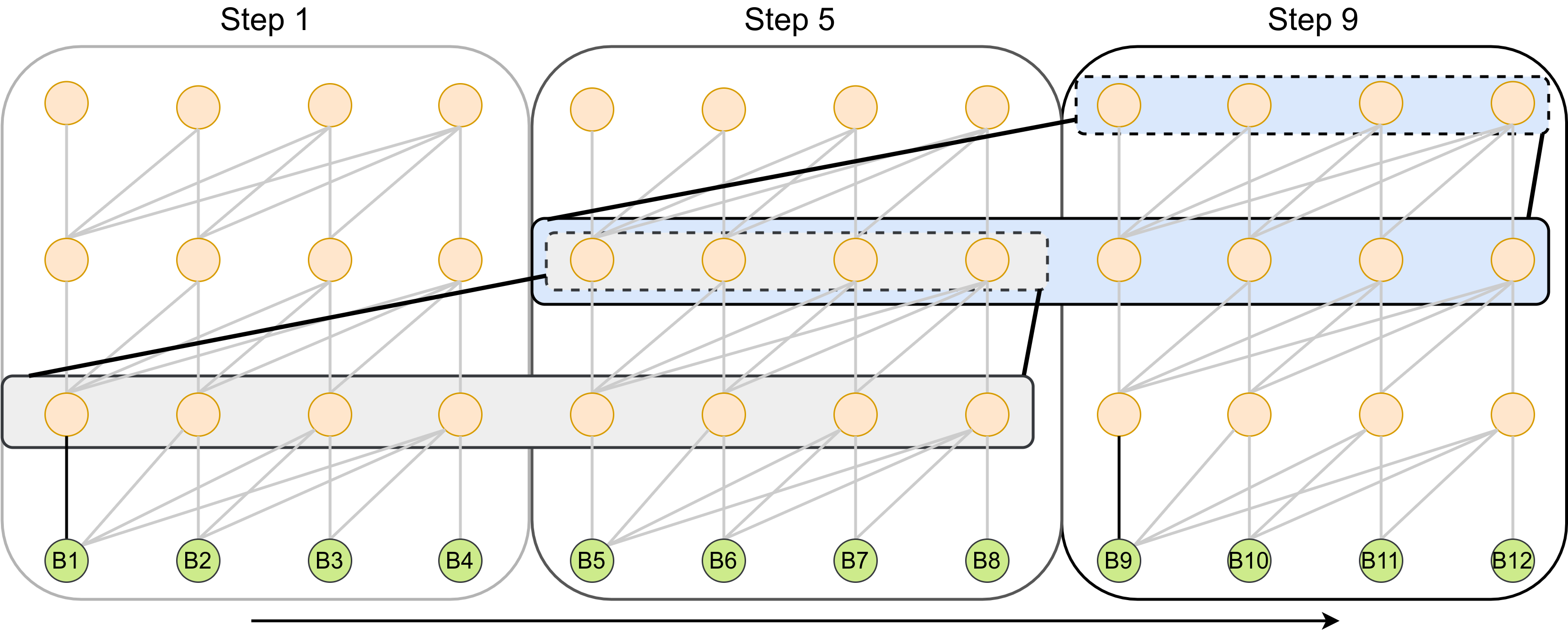
Figure 2: Demonstrating 3 layers of recurrent attention with a context size of 4. The solid lines joining layers show the information dependence flows in step 9, and the dotted line block is the attention result of the previous layer.

As shown in Fig. 2, by using the recurrence feature, the model can get the information of the previous $L-1$ context blocks, where $L$ denotes the layer number of the encoder. As a result, the recurrent attention encoder is able to achieve longer dependence with a smaller model size. Consequently, it is easy to design a suitable model that can receive useful information of all packed boxes visible on the upper surface of the bin when packing a new one. Besides, the model does not have to apply positional encoding as the packed state already contains position information that includes the sizes and coordinates of the packed boxes.

5.2 Conditional Query Decoder

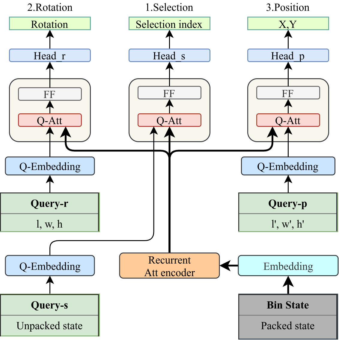
Figure 3: Recurrent Conditional Query Model.

After encoding the packed state into an embedded vector $\boldsymbol{h}_{e}^{n}$ by the recurrent attention encoder, we design the conditional query mechanism to handle the connection between sub-actions. As shown in Fig. 3, for packing problems, the model performs three sub-actions sequentially, namely, box selection, rotation and positioning for the selected box, and each sub-action has one independent decoder.

These three decoders have the same basic MHA structure, but their embedded conditional query signals that are from previous steps are different. They also share the same attention key and value as calculated by the recurrent attention encoder, which embed the information from the packed state. A conditional query layer contains a Queried MHA (Q-Att) and a Feed-Forward (FF) layer. After the conditional query layer, each decoder has several linear head layers to project the conditional query outputs $\boldsymbol{q}_{out}$ to each sub-action probability.

$$\begin{split}\boldsymbol{q}_{s}&=\boldsymbol{W}_{qs}^{T}(\boldsymbol{W}_{s}\boldsymbol{s}_{u}),\;\boldsymbol{q}_{r}=\boldsymbol{W}_{qr}^{T}(\boldsymbol{W}_{r}s_{c}),\;\boldsymbol{q}_{p}=\boldsymbol{W}_{qp}^{T}(\boldsymbol{W}_{p}s_{c}^{\prime})\\ \boldsymbol{q}_{o}&=\text{MHA}(\boldsymbol{q},\boldsymbol{W}_{k}^{T}\boldsymbol{h}_{e}^{n},\boldsymbol{W}_{v}^{T}\boldsymbol{h}_{e}^{n})\end{split}$$ (6)

To be more specific, as formulated in (6), the unpacked state $\boldsymbol{s}_{u}$ is embedded as a query vector $\boldsymbol{q}_{s}$ in the box selection step. After decoding, the candidate box is selected from boxes in the unpacked state, in which $\boldsymbol{W}_{s},\boldsymbol{W}_{r},\boldsymbol{W}_{p}$ are weight matrices of three sub-actions for query embedding. Then in the rotation step, the conditional query $\boldsymbol{q}_{r}$ is constructed by picking up the selected box shape information $s_{c}$ from the unpacked state and embedding it in a linear layer. The model calculates the position of the selected box relative to the bin in the final step. To incorporate all previous results, the positioning step query $s_{c}^{\prime}$ combines the rotation of the selected box.

Throughout the entire forward pass of packing one box, the data stream passes through the encoder and each decoder once. The target query is extracted from the candidate box state based on the previous outputs. Via the conditional query, the model receives information from the hidden vectors of the encoder as well as previous sub-action outputs, which ensures that every sub-action decoding step is an MDP.

5.3 Training

As mentioned earlier, we view the packing process as an MDP and apply reinforcement learning, or specifically, the actor-critic algorithm (Konda and Tsitsiklis, 2000). The model presented earlier is an actor model. Here we briefly describe the critic model, the actor policy and the training process.

5.3.1 The Critic Model

The critic structure is similar to the box selection model of the actor model, which consists of a recurrent attention encoder and a conditional decoder with the unpacked state as input followed by a value head. To make the training process more stable and easier to tune, we separate the actor network from the critic network, that is, the two networks do not share parameters. In addition, Generalized Advantage Estimation (GAE) (Schulman et al., 2016) is adopted in the action advantage $\hat{A}(s,a)$ estimation process to achieve stable and accurate advantage estimation.

5.3.2 The Policy

By modeling the problem as an MDP, each sub-action policy is independent of each other, and the policy is expressed in logarithmic form in the actor-critic algorithm. Therefore, as formulated in (7), the full packing step policy $\pi(a|s)$ is the product of sub-action policies, where subscripts $s,r,p$ denote box selection, rotation, and position sub-action, respectively.

$$\begin{split}\log\pi(a|s)&=\log\pi_{s}(a_{s}|s_{s})\pi_{r}(a_{r}|s_{r})\pi_{p}(a_{p}|s_{p})\\ &=\log\pi_{s}(a_{s}|s_{s})\!+\log\pi_{r}(a_{r}|s_{r})\!+\log\pi_{p}(a_{p}|s_{p})\end{split}$$ (7)

5.3.3 Training Process

In every training step, the critic network estimates the state values, and the actor network performs the three steps described before to get each sub-action output. Thereafter, one-step parameter update is performed for both the actor and critic networks. Because our training data is randomly generated and is inexpensive, the on-policy actor-critic algorithm is applied.

At the same time, choosing the optimal temperature $\alpha^{*}$ in (3) is non-trivial since the magnitude of the reward differs across tasks and also depends on the policy, which improves over time during training. So we also use an objective function for $\alpha$ and tune it automatically, where, like in SAC (Haarnoja et al., 2018), entropy is considered a constraint.

$$\begin{split}\mathcal{L}&=\mathcal{L}_{\theta}+\mathcal{L}_{\phi}+\mathcal{L}_{\alpha}\\ \mathcal{L}_{\theta}&=-\hat{A}(s_{t},a_{t})*\sum_{a\in\mathcal{A}}\log\pi_{\theta}(a_{t}|s_{t})\\ \mathcal{L}_{\phi}&=MSE[(V_{\phi}(s_{t}),\hat{A}(s_{t},a_{t})+V_{\phi}(s_{t})]\\ \mathcal{L}_{\alpha}&=\alpha_{t}[\bar{\mathcal{H}}-\log\pi_{t}(a_{t}|s_{t})]\end{split}$$ (8)

Equation (8) formulates the loss function calculation process, which includes the actor, critic and entropy regularization temperature loss functions. The logarithm of policy $\log\pi_{\theta}(a_{t}|s_{t})$ consists of three sub-action policies as shown in (7). The actor loss $\mathcal{L}_{\theta}$ is the advantage multiplying the policy gradient that encourages actions to achieve higher accumulate rewards. The critic network is trained through Mean Square Error (MSE) loss $\mathcal{L}_{\phi}$, in which $V_{\phi}(s_{t})$ is the value function estimation. The entropy regularization temperature loss $\mathcal{L}_{\alpha}$ keeps the policy entropy close to the target entropy $\bar{\mathcal{H}}$ to balance between exploitation and exploration.

6 Experiments

We evaluate the RCQL model on 2D and 3D strip packing problems, for both online and offline versions, with different packing box numbers and compare the results with heuristic algorithms and learning-based methods.

6.1 Experimental Setup

6.1.1 Packing Environment

In our packing problem environment, the model only needs to generate the index, rotation and the horizontal coordinates of the packing box at every packing step. Considering the gravitational property of boxes, the box should be supported by the bin or other boxes. Therefore, the environment will automatically drop the box $i$ to the lowest available position in the bin, which is formulated as $z_{i}=\max_{b}({z_{b}+h_{b}})$. The support box $b$ satisfies the following constrains:

$$x_{i} <x_{b}+w_{b}$$ (9)

$$x_{b} <x_{i}+w_{i}$$

$$y_{i} <y_{b}+l_{b}$$

$$y_{b} <y_{i}+l_{i}$$

in which $x,y,z$ denote the left-back-bottom coordinates of the box, and $w,l,h$ denote the box width, length, and height, respectively. The equation (9) ensures that box $b$ supports the upper box $i$. To avoid the model generating positions outside of the bin, as formulated in (10), the environment forces the cross-border boxes to the bin border, where $W,L$ denote the bin width and length, respectively. The number of discrete position slots $n_{s}$ is set to 128. We find this to be enough to obtain good packing results while it would not slow down the training process too much.

$$x_{i} =\min(x_{i},W-w_{i})$$ (10)

$$y_{i} =\min(y_{i},L-y_{i})$$

6.1.2 Dataset

In our packing environment, $N$ boxes are initialized with random width, length and height. The bin is initialized with a fixed width and length, and normalized to $-1\sim 1$, which can be easily scaled to any bin size. Unlike previous datasets, due to random sampling, the sizes of boxes here are strongly heterogeneous, which makes the problem harder. The agent has to find a solution sequence of candidate boxes using minimum bin height without any overlapping of boxes. In order to show the generalization ability of the methods, we evaluate the algorithms on one plain dataset ($w,l,h\sim U(0,L_{b})$) and one hard dataset ($w,l,h\sim U(0,L_{b}/4)$), where $L_{b}$ denotes the length and width of the bin.

There are two reasons for choosing randomly synthesized datasets. First, reinforcement learning requires lots of data to train. Thus, it is impractical to use real-world datasets in training. In fact, synthetic datasets are widely used in neural combinatorial optimization literature (Kool et al., 2019; Chen and Tian, 2019; Joshi et al., 2019; Xing and Tu, 2020). Second, our dataset is generated by uniform sampling, and we all know that the uniform distribution has the largest entropy, which means that it is the hardest one. Therefore, the results on this dataset can speak for the quality of the method.

6.1.3 Implementation Details

We experiment with two sizes of models. Our small models have 3 encoder layers and a decoder layer with a hidden size $d_{h}=128$, except the feedforward ReLU layers, which have 512 units. The large models have 6 encoder layers and 2 decoder layers with a hidden size $d_{h}=256$, and a feedforward size of 1024. All models have 8 attention heads in each layer. Each attention layer applies batch normalization. Compared with the model with no recurrence, the recurrent model can increase the context information from $B$ to $L*B$, where $L$ and $B$ are the number of encoder layers and the length of the recurrent FIFO, respectively. Therefore, we set $B$ as 20 based on the dataset and the model size to balance the performance and memory cost. Eventually, our small model has 2.16M parameters, while the large one has 4.24M parameters.

We use Adam (Kingma and Ba, 2015) with a batch size of 128 and a fixed learning rate of $10^{-4}$. The discount rate $\gamma$ is set as 0.96. We train our RCQL model on instances of 200 boxes with 10000 training steps and then evaluate it with a greedy decoder on various numbers of boxes to show the scalability of our model. We also adopt gradient clipping at 5.0 for better stability. The target entropy $\bar{\mathcal{H}}$ is set as 0.6 for automatic temperature adjustment. The model is trained on a single GeForce 2080Ti GPU. It takes about 2 days training for 3D offline cases.

6.1.4 Baselines

We compare our method with heuristic algorithms and learning-based methods. Here we choose the best heuristic methods that are currently known (Jylänki, 2010), MAXRECTS_BL for offline cases, and SKYLINE_BL for online cases. For meta-heuristic algorithms, a Genetic Algorithm (GA) (Wu et al., 2010) and a Simulated Annealing (SA) (Rakotonirainy and van Vuuren, 2020) one are tested. In GA, the population size and number of generations are 120 and 200 respectively. In SA, same as in the original paper, the search is terminated when 5000 search iterations has been carried out. For learning-based algorithms, the multi-task selected learning (MTSL) (Duan et al., 2019) model is evaluated. For comparison purpose, we implement their model but set the same reward function as ours. To verify the effectiveness of our conditional query mechanism, we remove the conditional query of our model (No query) and get the box rotation and position from the box selection decoder. Besides, we also test the rollout baseline (Kool et al., 2019) with the REINFORCE algorithm, which was claimed to be computationally more efficient.

6.2 Performance Evaluation

We evaluate previously mentioned algorithms by the bin gap ratio $\rho=(1-\frac{\sum_{i=1}^{n}w_{i}l_{i}h_{i}}{WLH_{n}})\times 100\%$, which is positively related to the final bin height. The variance of the bin gap ratio is also evaluated to show the stability of the learning algorithms. Because other learning-based methods cannot handle large scale packing problems, the case with 40 boxes is selected for comparison. Large scale problems are tested in the scalability evaluation part.

Table 1: Results in 40 boxes cases on hard dataset ($w,l,h\sim U(0,L_{b}/4)$). The variances of the learning methods are calculated from 4 inference runs, the batch size in each run is 128, and the variances of other methods are obtained from 512 separate runs.

	Method	Offline					Online
		Worst (%)	Best (%)	Average (%)	Variance	Time (ms)	Average (%)	Variance
2D	Heuristic	26.12	6.80	15.81	0.0018	11	21.11	0.0064
	GA	65.59	34.65	49.70	0.0026	1386	-	-
	SA	25.94	7.39	15.37	0.0017	12692	-	-
	Rollout	40.57	19.34	28.12	0.0021	439	-	-
	No query	38.26	17.98	25.73	0.0012	598	26.46	0.0003
	RCQL	27.34	9.74	14.56	0.0015	624	15.57	0.0003
	RCQL large	25.03	8.87	13.98	0.0020	978	14.86	0.0002
3D	Heuristic	63.29	34.16	46.37	0.0023	15	52.97	0.0072
	GA	72.72	45.51	59.57	0.0018	4312	-	-
	MTSL	70.56	45.87	54.29	0.0033	1924	-	-
	Rollout	57.67	30.97	38.09	0.0034	690	-	-
	No query	55.29	27.77	33.14	0.0025	765	49.83	0.0003
	RCQL	52.84	28.97	31.25	0.0012	828	48.37	0.0003
	RCQL large	49.23	27.12	30.25	0.0015	1037	46.12	0.0002

Table 1 shows numerical results of 512 instances with 40 boxes for both 2D and 3D cases. Our RCQL model achieves lower bin gap ratio in both 2D and 3D, online and offline cases. Specifically, in 2D cases, although the small RCQL model has only 2.49M parameters, it achieves 14.56% and 15.57% average gap ratios, in offline and online situations, respectively. The best heuristic algorithm shows superior performance to GA and learning-based baselines since it applies explicit rules that make boxes cling to each other and do not consider the gravitational property of boxes which makes the solution space larger than others. SA achieves a lower gap ratio than the heuristic one since it searches for better results among heuristic construction solutions. However, SA requires a lot of iterations to search from scratch, making the time cost of SA much higher. While our method already learned the packing pattern after training, it is faster than these meta-heuristic methods in inference time. For the 3D cases, learning-based approaches show lower gap ratios, and models which have the attention mechanism show better result than the others. The variance of the RCQL model is relatively small, which means that it can stably learn the general pattern of the packing problems. Furthermore, larger RCQL models also show slightly better results than small models.

It is clear that the model with the conditional query mechanism is better than the no query model, which confirms that the conditional query fills the information gap between sub-actions and makes the learning algorithm capable of reasoning for the following sub-actions according to the embedded previous outputs. Meanwhile, the rollout baseline with REINFORCE produces similar results to the no query model but with higher variance. Because the rollout method sums up all rewards in every packing step as the action value, its learning process treats every packing step equally and back-propagates gradients for all steps regardless of whether the quality of actions is good or bad. MTSL shows poor results, because their setting is only a partially observable MDP. Because of the information gap between sub-actions, MTSL also shows very high variance results.

Learning-based methods are slower than the heuristic algorithms since the computational load of NNs is relatively large. But it is faster than meta-heuristics, because the searching process of meta-heuristics is time-consuming. In addition, the NN model can benefit from batch input, so the time cost per input instance is much less than the time reported. Due to recurrence, the RCQL model is slightly slower than the other learning methods except MTSL in the 40 boxes case. But the baseline models can not handle large scale problems since the memory cost will be unbearable. While the time cost of the RCQL model is only linearly proportional to the box number owing to its recurrent feature. It only takes about 21 seconds when the number of boxes reaches 1000 and it achieves a 5.64% lower bin gap ratio than GA.

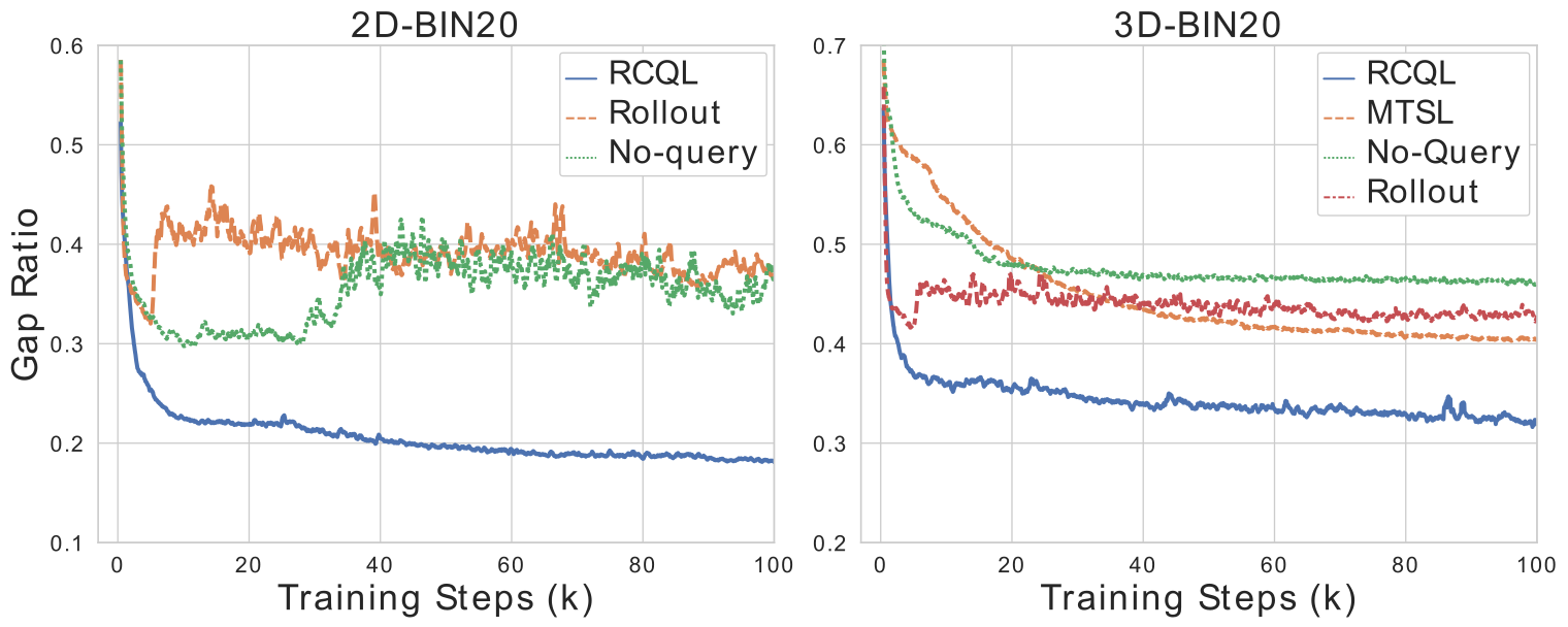
Figure 4: Learning curve of different models. Tested with the 20 boxes case.

From the learning curve of the training process shown in Fig. 4, the RCQL model also shows superior stability to the other learning algorithms, which leads to lower variance as shown in Table 1. The learning curve of the no query model is oscillating as the sampled results of earlier steps are not passed on to the later steps. That is, the model can only estimate the solution that is good overall but not one that fits the instance with specific input state. The learning curve of the rollout method shows a big spike at the beginning of training process because of the sudden baseline update after the first epoch. In contrast, the RCQL model benefits from conditional query to construct a strict MDP and has meaningful reward signals from every box packing step, so it gives a smooth convergence process.

6.3 Scalability Evaluation

In order to evaluate the scalability and generalization ability of these algorithms, we use different box numbers and different datasets in the experiments. Because no recurrence model must embed all box states to infer actions, the memory cost increases quadratically with the the increase of the box number. When the number exceeds 60, the baseline models all run out of GPU memory during training time. So we only evaluate these models for no more than 60 boxes. Another major drawback of these models is that their structures are problem size-related. As a result, for each problem instance with a certain number of boxes, a new model must be trained. In contrast, only one trained RCQL model is needed to handle various numbers of boxes; that is, 20 and 1000 boxes cases use the same RCQL model.

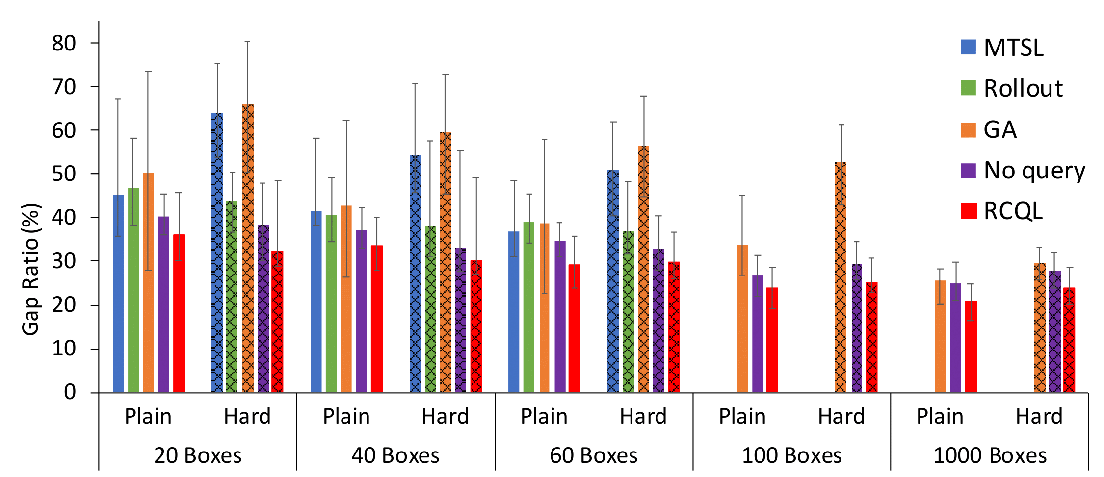
Figure 5: Bin gap ratio with different box numbers and datasets in 3D offline cases. Lower is better.

As shown in Fig. 5, the bin gap ratio of RCQL is lower than all the baseline ones for various datasets. The overall gap ratio of all methods decreases as the packing box number increases. The rollout and no query models show lower gap ratio than the other baselines, which means the attention models are more efficient in learning the packing pattern. RCQL achieves the highest space utilization ratio with only one trained model for all datasets and different box numbers. Although the genetic algorithm becomes better than MTSL when the box number increases, it is still inferior to RCQL since it tends to get trapped in local optima.

6.4 Training/Testing Generalization

To further study the generalization ability of the RCQL model, five models are trained through hard datasets with different instances sizes, which are then evaluated on testing sets with various instance sizes.

Table 2: Testing results of various sizes of RCQL models trained through different instance sizes.

Train	Test
	40	100	200	500	800	1000
40	32.43	29.27	27.95	25.79	25.56	26.50
100	31.36	27.47	24.50	23.97	22.90	22.84
200	31.25	27.97	24.98	22.92	22.18	22.11
500	34.94	28.96	25.45	23.10	22.06	21.79
800	37.40	32.71	26.88	23.37	22.30	22.48

As shown in Table 2, the bin gap ratios of different models tested on specific instance sizes come out to be very similar. In some cases, the model trained with different instance sizes performs even better than the one trained with the same instance size. This shows that test results do not rely on the instance sizes of the training sets, and the model can be satisfactorily generalized by learning the packing pattern.

Generally, when the instance size is larger, the bin gap ratio is lower. In particular, the model trained with 40-box instances results in a relatively high gap since it has no chance to learn the generalization ability of long-term dependency. In contrast, a model trained with too large an instance size will cause the Bellman backup (Greene et al., 2019) in value iteration to be non-trivial, which will also lead to performance degradation.

6.5 Going Deeper with Context

To study the effect of context information, we experiment with different context sizes of packed boxes $n_{p}$ and unpacked boxes $n_{u}$. The results are shown in Table 3, where two small models (3 encoder layers and 1 decoder layer) are trained in each specific context setting—one has recurrent connections, the other does not. The training GPU memory costs of these two models under specific $n_{p}$ and $n_{u}$ are similar, so we only report it in the recurrence case. Dynamic state updating is employed in both models.

Table 3: Empirical results for context size and recurrence. All models are trained and tested on 3D hard instances with 200 boxes. The training set contains $128*10^{4}$ instances.

$n_{u}$	$n_{p}$	Bin Gap Ratio $\rho$ (%)		GPU Memory (GB)
		W/ Recur	W/O Recur
10	5	33.91	34.66	1.758
	10	32.83	33.97	2.246
	20	32.58	30.61	3.184
20	5	29.24	32.27	2.064
	10	28.36	30.92	2.770
	20	25.98	26.95	3.586
30	10	26.84	31.72	2.830
	20	26.38	28.34	4.386
	30	24.25	26.56	5.172

As shown in Table 3, larger context sizes lead to lower bin gap ratio, which attests to the fact that more state information helps the learning of the effective packing strategies. If the recurrent connection is removed, the bin gap volume increases. The smaller the packed state context size $n_{p}$, the more evident would be the improvement of adding the recurrent connection. This is because a small $n_{p}$ would lose the long range context, which is important for constructing the MDP and the learning process. The recurrent connection extends the context length to $L*n_{p}$, where $L$ is the layer number of the recurrent encoder, which is 3 here. Specifically, the recurrence model bin gap ratio $\rho_{n_{u}=30,n_{p}=10}^{r}$ is 26.84, which is close to the gap ratio of the no-recurrence model $\rho_{n_{u}=30,n_{p}=30}^{nr}$ since they have same context size. Therefore, models with recurrent connections can achieve similar performance with lower memory costs.

Although a larger context size achieves better bin space utilization, the increase in memory overhead grows quadratically with the sequence length, as mentioned in Section 5.1. When the context size becomes larger, the performance improvement decreases as the unit context size increases, because the context with a long distance has little effect on the next packing action. Too large a context size also makes the training time unacceptable; in our tests, when both $n_{u}$ and $n_{p}$ were 50, it took several weeks to train and the training memory cost was about 11 GB. As a result, in previous evaluations, both $n_{u}$ and $n_{p}$ were set to 20 in order to strike a balance between optimality and training cost.

7 Conclusion

In this paper, we propose a recurrent conditional query learning method to solve packing problems. The RCQL model can be generalized to tackle any problem with mutually conditioned actions and can solve large scale strip packing problems with a small number of parameters. Numerical results show that the RCQL performs better than state-of-the-art methods for both 2D and 3D strip packing problems.

The success of RCQL proves that the conditional query mechanism is an efficient method for solving problems with parameterized action space. Besides, incorporating recurrent feature in NCO is an efficient way to handle large scale problems in operations research. The recurrent feature indeed has the potential to improve the scalability of NCO methods applied in other optimization problems such as routing.

References

- Christensen et al. [2017] Henrik I Christensen, Arindam Khan, Sebastian Pokutta, and Prasad Tetali. Approximation and online algorithms for multidimensional bin packing: A survey. Computer Science Review, 24:63–79, 2017.
- Martello et al. [2000] Silvano Martello, David Pisinger, and Daniele Vigo. The three-dimensional bin packing problem. Operations research, 48(2):256–267, 2000.
- Silva et al. [2019] Everton Fernandes Silva, Tony Wauters, et al. Exact methods for three-dimensional cutting and packing: A comparative study concerning single container problems. Computers & Operations Research, 109:12–27, 2019.
- Crainic et al. [2008] Teodor Gabriel Crainic, Guido Perboli, and Roberto Tadei. Extreme point-based heuristics for three-dimensional bin packing. Informs Journal on computing, 20(3):368–384, 2008.
- Baltacioglu et al. [2006] Erhan Baltacioglu, James T Moore, and Raymond R Hill Jr. The distributor’s three-dimensional pallet-packing problem: a human intelligence-based heuristic approach. International Journal of Operational Research, 1(3):249–266, 2006.
- Gonçalves and Resende [2011] José Fernando Gonçalves and Mauricio GC Resende. A parallel multi-population genetic algorithm for a constrained two-dimensional orthogonal packing problem. Journal of Combinatorial Optimization, 22(2):180–201, 2011.
- Egeblad and Pisinger [2009] Jens Egeblad and David Pisinger. Heuristic approaches for the two-and three-dimensional knapsack packing problem. Computers & Operations Research, 36(4):1026–1049, 2009.
- Duong [2015] Thai Ha Duong. Heuristics approaches for three-dimensional strip packing and multiple carrier transportation plans. PhD thesis, University of Nottingham, 2015.
- Wei et al. [2012] Lijun Wei, Wee-Chong Oon, Wenbin Zhu, and Andrew Lim. A reference length approach for the 3d strip packing problem. European Journal of Operational Research, 220(1):37–47, 2012.
- Wei et al. [2017] Lijun Wei, Qian Hu, Stephen CH Leung, and Ning Zhang. An improved skyline based heuristic for the 2d strip packing problem and its efficient implementation. Computers & Operations Research, 80:113–127, 2017.
- Rakotonirainy and van Vuuren [2020] Rosephine G Rakotonirainy and Jan H van Vuuren. Improved metaheuristics for the two-dimensional strip packing problem. Applied Soft Computing, 92:106268, 2020.
- Zeng et al. [2016] Zhizhong Zeng, Xinguo Yu, Kun He, Wenqi Huang, and Zhanghua Fu. Iterated tabu search and variable neighborhood descent for packing unequal circles into a circular container. European Journal of Operational Research, 250(2):615–627, 2016.
- Mostaghimi Ghomi et al. [2017] Hanan Mostaghimi Ghomi, Bryan Gary St Amour, and Walid Abdul-Kader. Three-dimensional container loading: A simulated annealing approach. International Journal of Applied Engineering Research, 12(7):1290, 2017.
- Wu et al. [2010] Yong Wu, Wenkai Li, Mark Goh, and Robert de Souza. Three-dimensional bin packing problem with variable bin height. European journal of operational research, 202(2):347–355, 2010.
- Bello et al. [2016] Irwan Bello, Hieu Pham, Quoc V Le, Mohammad Norouzi, and Samy Bengio. Neural combinatorial optimization with reinforcement learning. In International Conference on Learning Representations, 2016.
- Nazari et al. [2018] Mohammadreza Nazari, Afshin Oroojlooy, Lawrence Snyder, and Martin Takác. Reinforcement learning for solving the vehicle routing problem. In Advances in Neural Information Processing Systems, pages 9839–9849, 2018.
- Lu et al. [2019] Hao Lu, Xingwen Zhang, and Shuang Yang. A learning-based iterative method for solving vehicle routing problems. In International Conference on Learning Representations, 2019.
- Duan et al. [2019] Lu Duan, Haoyuan Hu, Yu Qian, Yu Gong, Xiaodong Zhang, Jiangwen Wei, and Yinghui Xu. A multi-task selected learning approach for solving 3d flexible bin packing problem. In Proceedings of the 18th International Conference on Autonomous Agents and MultiAgent Systems, pages 1386–1394, 2019.
- Cai et al. [2019] Qingpeng Cai, Will Hang, Azalia Mirhoseini, George Tucker, Jingtao Wang, and Wei Wei. Reinforcement learning driven heuristic optimization. In Workshop on Deep Reinforcement Learning for Knowledge Discovery, 2019.
- Sutton and Barto [2018] Richard S Sutton and Andrew G Barto. Reinforcement learning: An introduction. MIT press, 2018.
- Haarnoja et al. [2018] Tuomas Haarnoja, Aurick Zhou, Pieter Abbeel, and Sergey Levine. Soft actor-critic: Off-policy maximum entropy deep reinforcement learning with a stochastic actor. In International Conference on Machine Learning, pages 1861–1870, 2018.
- Andrychowicz et al. [2017] Marcin Andrychowicz, Filip Wolski, Alex Ray, Jonas Schneider, Rachel Fong, Peter Welinder, Bob McGrew, Josh Tobin, OpenAI Pieter Abbeel, and Wojciech Zaremba. Hindsight experience replay. In Advances in Neural Information Processing Systems, pages 5048–5058, 2017.
- Baldi et al. [2019] Mauro Maria Baldi, Daniele Manerba, Guido Perboli, and Roberto Tadei. A generalized bin packing problem for parcel delivery in last-mile logistics. European Journal of Operational Research, 274(3):990–999, 2019.
- Ding et al. [2019] Tao Ding, Jiawen Bai, Pengwei Du, Boyu Qin, Furong Li, Jin Ma, and Zhaoyang Dong. Rectangle packing problem for battery charging dispatch considering uninterrupted discrete charging rate. IEEE Transactions on Power Systems, 34(3):2472–2475, 2019.
- Grange et al. [2018] Aristide Grange, Imed Kacem, and Sébastien Martin. Algorithms for the bin packing problem with overlapping items. Computers & Industrial Engineering, 115:331–341, 2018.
- Martinez-Sykora et al. [2017] Antonio Martinez-Sykora, Ramón Alvarez-Valdés, Julia A Bennell, R Ruiz, and José Manuel Tamarit. Matheuristics for the irregular bin packing problem with free rotations. European Journal of Operational Research, 258(2):440–455, 2017.
- Kool et al. [2019] Wouter Kool, Herke van Hoof, and Max Welling. Attention, learn to solve routing problems! In International Conference on Learning Representations, 2019.
- Schulman et al. [2016] John Schulman, Philipp Moritz, Sergey Levine, Michael Jordan, and Pieter Abbeel. High-dimensional continuous control using generalized advantage estimation. In International Conference on Learning Representations, 2016.
- Bahdanau et al. [2015] Dzmitry Bahdanau, Kyunghyun Cho, and Yoshua Bengio. Neural machine translation by jointly learning to align and translate. In International Conference on Learning Representations, 2015.
- Vinyals et al. [2016] Oriol Vinyals, Samy Bengio, and Manjunath Kudlur. Order matters: Sequence to sequence for sets. In International Conference on Learning Representations, 2016.
- Luong et al. [2015] Thang Luong, Hieu Pham, and Christopher D Manning. Effective approaches to attention-based neural machine translation. In Proceedings of the 2015 Conference on Empirical Methods in Natural Language Processing, pages 1412–1421, 2015.
- Vaswani et al. [2017] Ashish Vaswani, Noam Shazeer, Niki Parmar, Jakob Uszkoreit, Llion Jones, Aidan N Gomez, Łukasz Kaiser, and Illia Polosukhin. Attention is all you need. In Advances in neural information processing systems, pages 5998–6008, 2017.
- Shen et al. [2018] Tao Shen, Tianyi Zhou, Guodong Long, Jing Jiang, and Chengqi Zhang. Bi-directional block self-attention for fast and memory-efficient sequence modeling. In International Conference on Learning Representations, 2018.
- Wang et al. [2016] Tong Wang, Ping Chen, John Rochford, and Jipeng Qiang. Text simplification using neural machine translation. In Proceedings of the AAAI Conference on Artificial Intelligence, volume 30, 2016.
- Mazyavkina et al. [2021] Nina Mazyavkina, Sergey Sviridov, Sergei Ivanov, and Evgeny Burnaev. Reinforcement learning for combinatorial optimization: A survey. Computers & Operations Research, page 105400, 2021.
- Vinyals et al. [2015] Oriol Vinyals, Meire Fortunato, and Navdeep Jaitly. Pointer networks. In Advances in Neural Information Processing Systems, pages 2692–2700, 2015.
- Masson et al. [2016] Warwick Masson, Pravesh Ranchod, and George Konidaris. Reinforcement learning with parameterized actions. In Thirtieth AAAI Conference on Artificial Intelligence, 2016.
- Fan et al. [2019] Zhou Fan, Rui Su, Weinan Zhang, and Yong Yu. Hybrid actor-critic reinforcement learning in parameterized action space. In Proceedings of the 28th International Joint Conference on Artificial Intelligence, pages 2279–2285, 2019.
- Neunert et al. [2020] Michael Neunert, Abbas Abdolmaleki, Markus Wulfmeier, Thomas Lampe, Tobias Springenberg, Roland Hafner, Francesco Romano, Jonas Buchli, Nicolas Heess, and Martin Riedmiller. Continuous-discrete reinforcement learning for hybrid control in robotics. In Conference on Robot Learning, pages 735–751, 2020.
- Hausknecht and Stone [2016] Matthew Hausknecht and Peter Stone. Deep reinforcement learning in parameterized action space. In International Conference on Learning Representations, 2016.
- Silver et al. [2014] David Silver, Guy Lever, Nicolas Heess, Thomas Degris, Daan Wierstra, and Martin Riedmiller. Deterministic policy gradient algorithms. In International conference on machine learning, pages 387–395. PMLR, 2014.
- Xu et al. [2016] Bing Xu, Ruitong Huang, and Mu Li. Revise saturated activation functions. In International Conference on Learning Representations Workshop, 2016.
- Wei et al. [2018] Ermo Wei, Drew Wicke, and Sean Luke. Hierarchical approaches for reinforcement learning in parameterized action space. In 2018 AAAI Spring Symposium Series, 2018.
- Kingma et al. [2015] Durk P Kingma, Tim Salimans, and Max Welling. Variational dropout and the local reparameterization trick. Advances in neural information processing systems, 28:2575–2583, 2015.
- Child et al. [2019] Rewon Child, Scott Gray, Alec Radford, and Ilya Sutskever. Generating long sequences with sparse transformers. arXiv preprint arXiv:1904.10509, 2019.
- Dai et al. [2019] Zihang Dai, Zhilin Yang, Yiming Yang, Jaime G Carbonell, Quoc Le, and Ruslan Salakhutdinov. Transformer-xl: Attentive language models beyond a fixed-length context. In Proceedings of the 57th Annual Meeting of the Association for Computational Linguistics, pages 2978–2988, 2019.
- Konda and Tsitsiklis [2000] Vijay R Konda and John N Tsitsiklis. Actor-critic algorithms. In Advances in neural information processing systems, pages 1008–1014, 2000.
- Chen and Tian [2019] Xinyun Chen and Yuandong Tian. Learning to perform local rewriting for combinatorial optimization. In Advances in Neural Information Processing Systems, pages 6281–6292, 2019.
- Joshi et al. [2019] Chaitanya K Joshi, Thomas Laurent, and Xavier Bresson. An efficient graph convolutional network technique for the travelling salesman problem. arXiv preprint arXiv:1906.01227, 2019.
- Xing and Tu [2020] Zhihao Xing and Shikui Tu. A graph neural network assisted monte carlo tree search approach to traveling salesman problem. IEEE Access, 8:108418–108428, 2020.
- Kingma and Ba [2015] Diederik P Kingma and Jimmy Ba. Adam: A method for stochastic optimization. In ICLR (Poster), 2015.
- Jylänki [2010] Jukka Jylänki. A thousand ways to pack the bin-a practical approach to two-dimensional rectangle bin packing, 2010. URL http://clb.demon.fi/files/RectangleBinPack.pdf.
- Greene et al. [2019] Max L Greene, Patryk Deptula, Scott Nivison, and Warren E Dixon. Reinforcement learning with sparse bellman error extrapolation for infinite-horizon approximate optimal regulation. In IEEE Conference on Decision and Control (CDC), pages 1959–1964. IEEE, 2019.