A new technique for compression of data sets

Abstract

Data compression techniques are characterized by four key performance indices which are (i) associated accuracy, (ii) compression ratio, (iii) computational work, and (iv) degree of freedom. The method of data compression developed in this paper allows us to substantially improve all the four issues above.

The proposed transform $\cal F$ is presented in the form of a sum with $p-1$ terms, $\mbox{$\cal F$}_{1},\ldots,\mbox{$\cal F$}_{p-1}$, where each term is a particular sub-transform presented by a first degree polynomial. For $j=1,\ldots,p-1$, each sub-transform $\mbox{$\cal F$}_{j}$ is determined from interpolation-like conditions. This device provides the transform flexibility to incorporate variation of observed data and leads to performance improvement. The transform $\cal F$ has two degrees of freedom, the number of sub-transforms and associated compression ratio associated with each sub-transform $\mbox{$\cal F$}_{j}$.

1 Introduction

In this paper, a new technique for compression of a set of random signals is proposed. The technique provides the better associated accuracy, compression ratio and computational load than the Karhunen-Loève transform (KLT) and its known extensions.

The basic idea is to combine the methodologies of a piece-wise liner function interpolation [1] and the best rank-constrained operator approximation. This issue is discussed in more detail in Sections 2 and 3.

The KLT is the fundamental and, perhaps, most popular data compression method [2]–[12]. It is also known as the Principal Component Analysis (PCA) [13, 11] and “is probably the oldest and best known of the techniques of multivariate analysis” [13]. This technique is intensively used in a vide range of research areas such as data compression [14, 15], pattern recognition [16], interference suppression [17], image processing [18], forecasting [19], hydrology [20], physics nonlinear phenomena [21], probabilistic mechanics [22, 23], biomechanics [24], geoscience [25, 26], stochastic processes [27, 28], information theory [29, 30], 3-D object classification and video coding [31], chemical theory [32], oceanology [33], optics and laser technology [34] and others.

The purpose of techniques based on the KLT is to compress observable data vector $\mathbf{y}$ with $n$ components to a shorter vector $\widetilde{\mbox{$\mathbf{x}$}}$ with $r$ components (also called the principal components [13]) and then reconstruct it so that the reconstruction is close to the reference signal $\mathbf{x}$. In general, $\mathbf{x}$ contains $m$ components where $m$ is not necessarily equal to $n$. The ratio

$$c=\frac{r}{m},\quad\mbox{where $r\leq m$,}$$

is called the compression ratio. Smaller $r$ implies poorer accuracy in the reconstruction of the compressed data. In this sense, $r$ is the KLT degree of freedom. Therefore, the performance of the KLT and related transforms is characterized by four key performance indices which are (i) associated accuracy, (ii) compression ratio, (iii) computational work and (iv) the degree of freedom.

The method of data compression developed in this paper allows us to substantially (i) increase the accuracy, (ii) improve the compression ratio, (iii) decrease computational work and (iv) increase the degrees of freedom.

1.1 Motivations for the proposed technique

The motivations of the proposed are as follows.

1.1.1 Infinite sets of signals

Most of the literature on the subject of the KLT discusses the properties of an optimal transform for an individual finite random signal. This means that if one wishes to compress and then reconstruct an infinite set of observable signals $K_{{}_{Y}}=\{\mbox{$\mathbf{y}$}_{1},\mbox{$\mathbf{y}$}_{2},\ldots,\mbox{$\mathbf{y}$}_{N},\ldots\}$ so that reconstructed signals are close to an infinite set of reference random signals $K_{{}_{X}}=\{\mbox{$\mathbf{x}$}_{1},\mbox{$\mathbf{x}$}_{2},\ldots,\mbox{$\mathbf{x}$}_{N},\ldots\}$ using the KLT approach then one is forced to find an infinite set of corresponding transforms $\{\mbox{$\cal T$}_{1},\mbox{$\cal T$}_{2},\ldots,\mbox{$\cal T$}_{N},\ldots\}$: one element $\mbox{$\cal T$}_{i}$ of the transform set for each representative $\mbox{$\mathbf{y}$}_{i}$ of the signal set $K_{{}_{Y}}$. Clearly, such an approach cannot be applied in practice. Although the standard KLT has been extended in [9] to the cases of infinite signal sets, its associated accuracy is still not satisfactory (see Sections 1.1.3, 4.8 and 5).

1.1.2 Computational work

Note that even in the case when $K_{{}_{Y}}=\{\mbox{$\mathbf{y}$}_{1},\mbox{$\mathbf{y}$}_{2},\ldots,$ $\mbox{$\mathbf{y}$}_{N}\}$ and $K_{{}_{X}}=\{\mbox{$\mathbf{x}$}_{1},\mbox{$\mathbf{x}$}_{2},\ldots,\mbox{$\mathbf{x}$}_{N}\}$ with $N$ fixed can be represented as finite ‘long’ signals, the KLT applied to such signals leads to computation of large covariance matrices. Indeed, if each $\mbox{$\mathbf{y}$}_{i}$ has $n$ components and each $\mbox{$\mathbf{x}$}_{i}$ has $m$ components then the KLT approach leads to computation of a product of an $mN\times nN$ matrix and an $nN\times nN$ matrix and computation of a $nN\times nN$ pseudo-inverse matrix [7]. This requires $O(2mn^{2}N^{3})$ and $O(22n^{3}N^{3})$ flops, respectively [35]. As a result, in this case, the computational work associated with the KLT approach becomes unreasonably hard.

1.1.3 Associated accuracy

For the given compression ratio, the accuracy associated with the KLT-like techniques cannot be changed. If the accuracy is not satisfactory then one has to change the compression ratio, which can be undesirable. Thus, for the KLT approach, the compression ratio is the only degree of freedom to improve the accuracy.

1.2 Brief description of the KLT

First, we need some notation as follows. Let $X=(\Omega,\Sigma,\mu)$ be a probability space, where $\Omega=\{\omega\}$ is the set of outcomes, $\Sigma$ a $\sigma$–field of measurable subsets in $\Omega$ and $\mu:\Sigma\rightarrow[0,1]$ an associated probability measure on $\Sigma$.

Let $\mbox{$\mathbf{x}$}\in L^{2}(\Omega,{\mathbb{R}}^{n})$ and $\mbox{$\mathbf{y}$}\in L^{2}(\Omega,{\mathbb{R}}^{m})$ be a reference signal and an observed signal, respectively. Let the norm $\|\cdot\|^{2}_{\Omega}$ be given by $\displaystyle\|\mbox{$\mathbf{x}$}\|^{2}_{\Omega}={\int}_{\Omega}\|\mbox{$\mathbf{x}$}(\omega)\|^{2}_{2},d\mu(\omega)$ where $\|\mbox{$\mathbf{x}$}(\omega)\|_{2}$ is the Euclidean norm of $\mbox{$\mathbf{x}$}(\omega)\in{\mathbb{R}}^{m}$.

We consider a linear operator (transform) $\mbox{$\cal K$}:$ $L^{2}(\Omega,{\mathbb{R}}^{m})$ $\rightarrow L^{2}(\Omega,{\mathbb{R}}^{n})$ defined by a matrix $K\in\mbox{$\mathbb{R}$}^{m\times n}$ so that

$$[\mbox{$\cal K$}(\mbox{$\mathbf{y}$})](\omega)=K[\mbox{$\mathbf{y}$}(\omega)].$$ (1)

A generic KLT [7] is the linear transform $\cal K$ that solves

$$\min_{\mathbb{K}}\|\mbox{$\mathbf{x}$}-\mbox{$\cal K$}(\mbox{$\mathbf{y}$})\|^{2}_{\Omega}\quad\mbox{subject to $\mathrm{rank\;}\mbox{$\cal K$}=r\leq\min\{m,n\}$},$$ (2)

where $\mathbb{K}$ is a class of all linear operators defined by (1). As a result, the KLT returns two matrices, $D\in\mbox{$\mathbb{R}$}^{m\times r}$ and $C\in\mbox{$\mathbb{R}$}^{r\times n}$, so that $K=DC$. Matrix $C$ performs filtering and compression of observed data $\mathbf{y}$ to a shorter vector $\widetilde{\mbox{$\mathbf{x}$}}\in L^{2}(\Omega,{\mathbb{R}}^{r})$ with $r$ components. Matrix $D$ reconstructs $\widetilde{\mbox{$\mathbf{x}$}}$ in such a way that the reconstructed signal is close to $\mathbf{x}$ in the sense of (2).

Operator $\cal K$ that solves (2) for a particular case with $\mbox{$\mathbf{y}$}=\mbox{$\mathbf{x}$}$ is the standard KLT.

Thus, for a given compression ratio, the KLT minimizes the associated error over the class of all linear transforms of the rank defined by (2).

1.3 Related techniques

Despite the known KLT optimality, it may happen that the accuracy and compression ratio associated with the KLT are still not satisfactory. Owing to this observation and the KLT versatility in applications (see Section 1 above), the KLT idea was extended in different directions as has been done, in particular, in [2]–[6]. More recent developments in this area include the polynomial transforms [7], extensions of the KLT to the cases of infinite signal sets [9], the best weighted estimators [10, 11], distributed KLT [29] and the fast KLT using wavelets [36].

Nevertheless, the known transforms based on the KLT idea still imply intrinsic difficulties associated with the original KLT. In particular, most of them have been developed for the case of a single signal, and for the fixed compression ratio, the associated error cannot be improved. In the case of the polynomial transforms [7], the error can be improved if the number of terms in the polynomial transforms increase. The latter implies a substantial computational burden that, in many cases, may stifle this intention.

1.4 Contribution. Particular features of the proposed transform

To describe the contribution and compare the features of the proposed transform with those of the KLT-like techniques, we consider the same issues as in Section 1.1.

1.4.1 Infinite sets of signals

Unlike most of the known transforms, the proposed technique allows us to determine a single transform to compress any signal from the infinite signal set. We note that infinite sets of stochastic signal-vectors introduced in Section 2.2 are quite large and include, for example, time series.

1.4.2 Computational work

In the case of finite signal sets, the proposed technique requires a lesser computational load compared to the KLT approach (see Sections 4.8.3 and 5).

1.4.3 Associated accuracy

Our transform provides data compression and subsequent reconstruction with any desired accuracy (Theorem 3 in Section 4.4). This is achieved due to the transform structure that follows from the device of the piece-wise function interpolation (Sections 2.2 and 3). In particular, it provides the related degree of freedom, the number of the so-called interpolation pairs (see Sections 3 and 4.8.2), to improve the transform performance (Section 4.8).

Moreover, the proposed technique

(i) determines the data compression transform in terms of pseudo-inverse matrices so that the transform always exists,

(ii) uses the same initial information (signal samples) as is used in the KLT-like transforms (see Sections 4.5 and 5), and

(iii) provides the simultaneous filtering and compression.

The paper is organized as follows. In Section 2, a brief description of the problem is given. Some necessary preliminaries, used in our transform construction, are given in Section 2.2. In Section 2.2.2, the transform model $\cal F$ is provided. In Section 3, a rigorous statement of the problem is given, which is a generalization and extension of problem (2) to the case of filtering of infinite sets of stochastic signals. In Section 4, the proposed transform $F$ is determined from interpolation conditions, and the associated error analysis is presented. In particular, in Section 4.8, a comparison with KLT-like approach is given.

2 Underlying idea. Device of the transform

2.1 Underlying idea

In this paper, the underlying idea is different from those considered in the above mentioned works. The proposed transform is constructed from a combination of the device of the piece-wise linear function interpolation [1] and the best rank-constrained operator approximation. This means the following.

Suppose, $K_{{}_{Y}}$ and $K_{{}_{X}}$ are uncountable sets of random signals. While the rigorous notation is given in Section 2.2, here, we denote $\mbox{$\mathbf{y}$}(t,\cdot)\in K_{{}_{Y}}$ and $\mbox{$\mathbf{x}$}(t,\cdot)\in K_{{}_{X}}$ where $t\in[a\hskip 5.69054ptb]\subset\mbox{$\mathbb{R}$}$ is a time snapshot. Let $a=t_{1}\leq\ldots\leq t_{p}=b.$ Choose finite numbers of signals, $\{\mbox{$\mathbf{y}$}(t_{1},\cdot),\ldots,\mbox{$\mathbf{y}$}(t_{p},\cdot)\}\subset K_{{}_{Y}}$ and $\{\mbox{$\mathbf{x}$}(t_{1},\cdot),\ldots,\mbox{$\mathbf{x}$}(t_{p},\cdot)\}\subset K_{{}_{X}}$. The proposed transform $\cal F$ contains $p-1$ terms $\mbox{$\cal F$}_{1},\ldots,\mbox{$\cal F$}_{p-1}$ (see (5)–(6) below) where, for $j=1,\ldots,p-1$, each term $\mbox{$\cal F$}_{j}$ is given as a first order operator polynomial (see (6) below) and is determined from the interpolation conditions

$$\mbox{$\cal F$}_{j}[\mbox{$\mathbf{y}$}(t_{j},\cdot)]=\mbox{$\mathbf{x}$}(t_{j},\cdot)\hskip 5.69054pt\mbox{and}\hskip 5.69054pt\mbox{$\cal F$}_{j}[\mbox{$\mathbf{y}$}(t_{j+1},\cdot)]\approx\mbox{$\mathbf{x}$}(t_{j+1},\cdot).$$ (3)

A reason for using the approximate equality in (3) is explained in Section 3.3. In Section 3.1, the second condition in (3) is represented as the best rank-constrained approximation problem (11)–(12). As a result, such a transform has advantages that are similar to the known advantages of the piece-wise function interpolation as has been mentioned in Section 1.4. The procedure of data compression-reconstruction is performed via $p-1$ truncated singular value decompositions (SVD) provided in Section 4.3.

2.2 Device of the transform

2.2.1 Signal sets under consideration

We wish to consider signals in some wide sense as follows. Let $T:=[a,\hskip 2.84526ptb]\subseteq\mbox{$\mathbb{R}$}$, and let $K_{{}_{X}}$ and $K_{{}_{Y}}$ be infinite sets of signals,
$K_{{}_{X}}=\{\mbox{$\mathbf{x}$}(t,\cdot)\in L^{2}(\Omega,{\mathbb{R}}^{m})\hskip 2.84526pt|\hskip 2.84526ptt\in T\}$ and $K_{{}_{Y}}=\{\mbox{$\mathbf{y}$}(t,\cdot)$ $\in L^{2}(\Omega,{\mathbb{R}}^{n})\hskip 2.84526pt|\hskip 2.84526ptt\in T\}$ where

$$\mbox{$\mathbf{x}$}(t,\cdot)=[\mbox{$\mathbf{x}$}^{(1)}(t,\cdot)\ldots\mbox{$\mathbf{x}$}^{(m)}(t,\cdot)]^{T}$$

$$\mbox{with}\quad\mbox{$\mathbf{x}$}^{(j)}(t,\cdot)\in L^{2}(\Omega,{\mathbb{R}})\quad\forall\quad j=1,\ldots,m,$$

and

$$\mbox{$\mathbf{y}$}(t,\cdot)=[\mbox{$\mathbf{y}$}^{(1)}(t,\cdot)\ldots\mbox{$\mathbf{y}$}^{(n)}(t,\cdot)]^{T}$$

$$\mbox{with}\quad\mbox{$\mathbf{y}$}^{(i)}(t,\cdot)\in L^{2}(\Omega,{\mathbb{R}})\quad\forall\quad j=1,\ldots,n,$$

respectively.

We interpret $\mbox{$\mathbf{x}$}(t,\cdot)$ as a reference signal and $\mbox{$\mathbf{y}$}(t,\cdot)$ as an observable signal.

The variable $t\in T$ represents time. Then, for example, $\mbox{$\mathbf{x}$}(t,\cdot)$ can be interpreted as an arbitrary stationary time series.

Let $\{t_{k}\}_{1}^{p}\subset T$ be a nondecreasing sequence of fixed time-points such that

$$a=t_{1}\leq\ldots\leq t_{p}=b.$$ (4)

2.2.2 The transform model

Now let $\mbox{$\cal F$}:L^{2}(\Omega,\mbox{$\mathbb{R}$}^{n})\rightarrow L^{2}(\Omega,\mbox{$\mathbb{R}$}^{m})$ be a transform such that, for each $t\in T$,

$$\mbox{$\cal F$}[\mbox{$\mathbf{y}$}(t,\cdot)]=\sum_{j=1}^{p-1}\delta_{j}\mbox{$\cal F$}_{j}[\mbox{$\mathbf{y}$}(t,\cdot)],$$ (5)

where

$$\mbox{$\cal F$}_{j}[\mbox{$\mathbf{y}$}(t,\cdot)]=\mbox{$\mathbf{a}$}_{j}+\mbox{$\cal G$}_{j}[\mbox{$\mathbf{y}$}(t,\cdot)]\hskip 5.69054pt\mbox{and}\hskip 5.69054pt\delta_{j}=\left\{\begin{array}[]{cl}1,&\mbox{if $t_{j}\leq t\leq t_{j+1}$},\\ 0,&\mbox{otherwise.}\end{array}\right.$$ (6)

Here, $\mbox{$\cal F$}_{j}$ is a sub-transform with $\mbox{$\mathbf{a}$}_{j}\in L^{2}(\Omega,\mbox{$\mathbb{R}$}^{m})$ and $\mbox{$\cal G$}_{j}:L^{2}(\Omega,\mbox{$\mathbb{R}$}^{n})\rightarrow L^{2}(\Omega,\mbox{$\mathbb{R}$}^{m})$ is a linear operator represented by a matrix $G_{j}\in\mbox{$\mathbb{R}$}^{m\times n}$ so that

$$[\mbox{$\cal G$}_{j}(\mbox{$\mathbf{y}$})](t,\omega)=G_{j}[\mbox{$\mathbf{y}$}(t,\omega)].$$

For each $j=1,\ldots,p-1$, vector $\mbox{$\mathbf{a}$}_{j}$ and operator $\mbox{$\cal G$}_{j}$ should be determined from the interpolation conditions given in the following Section 3.

Thus, $\mbox{$\cal F$}_{j}$ is defined by a matrix $F_{j}\in\mbox{$\mathbb{R}$}^{m\times n}$ such that

$$F_{j}[\mbox{$\mathbf{y}$}(t,\omega)]=\mbox{$\mathbf{a}$}_{j}(\omega)+G_{j}[\mbox{$\mathbf{y}$}(t,\omega)].$$ (7)

3 Statement of the problem

Let $\mbox{$\mathbf{x}$}(t_{1},\cdot),\ldots,\mbox{$\mathbf{x}$}(t_{p},\cdot)$ and $\mbox{$\mathbf{y}$}(t_{1},\cdot),\ldots,\mbox{$\mathbf{y}$}(t_{p},\cdot)$ be signals chosen from infinite signal sets $K_{{}_{X}}$ and $K_{{}_{Y}}$.

3.1 Preliminaries

Ideally, in (5)–(7), for $j=1,\ldots,p-1$, we would like to determine each $\mbox{$\cal F$}_{j}$ so that $\mbox{$\mathbf{a}$}_{j}$ satisfies

$$\mbox{$\mathbf{a}$}_{j}+\mbox{$\cal G$}_{j}[\mbox{$\mathbf{y}$}(t_{j},\cdot)]=\mbox{$\mathbf{x}$}(t_{j},\cdot)$$ (8)

and $\mbox{$\cal G$}_{j}$ solves

$$\mbox{$\mathbf{a}$}_{j}+\mbox{$\cal G$}_{j}[\mbox{$\mathbf{y}$}(t_{j+1},\cdot)]=\mbox{$\mathbf{x}$}(t_{j+1},\cdot).$$ (9)

The conditions (8)–(9) are motivated by the device of piece-wise function interpolation and associated advantages [1]. In turn, (8) implies $\mbox{$\mathbf{a}$}_{j}=\mbox{$\mathbf{x}$}(t_{j},\cdot)-\mbox{$\cal G$}_{j}[\mbox{$\mathbf{y}$}(t_{j},\cdot)]$ which being substituted in (9), reduces (9) to

$$\mbox{\tiny$\Delta$}\mbox{$\mathbf{x}$}(t_{j},t_{j+1},\cdot)-\mbox{$\cal G$}_{j}[\mbox{\tiny$\Delta$}\mbox{$\mathbf{y}$}(t_{j},t_{j+1},\cdot)]=\theta,$$ (10)

where

$$\mbox{\tiny$\Delta$}\mbox{$\mathbf{x}$}(t_{j},t_{j+1},\cdot)=\mbox{$\mathbf{x}$}(t_{j+1},\cdot)-\mbox{$\mathbf{x}$}(t_{j},\cdot),$$

$$\mbox{\tiny$\Delta$}\mbox{$\mathbf{y}$}(t_{j},t_{j+1},\cdot)=\mbox{$\mathbf{y}$}(t_{j+1},\cdot)-\mbox{$\mathbf{y}$}(t_{j},\cdot)$$

and $\theta$ is the zero vector.

Nevertheless, the transform $\cal F$ with such $\mbox{$\mathbf{a}$}_{j}$ and $\mbox{$\cal G$}_{j}$ does not provide data compression. To provide compression, we require that instead of (10), $\mbox{$\cal G$}_{j}$ solves

$$\min_{\small\mbox{$\cal G$}_{j}}\left\|\mbox{\tiny$\Delta$}\mbox{$\mathbf{x}$}(t_{j},t_{j+1},\cdot)-\mbox{$\cal G$}_{j}[\mbox{\tiny$\Delta$}\mbox{$\mathbf{y}$}(t_{j},t_{j+1},\cdot)]\right\|^{2}_{\Omega}$$ (11)

subject to

$$\mathrm{rank\;}\mbox{$\cal G$}_{j}=r_{j}\leq\min\{m,n\}.$$ (12)

In (11), we use the notation

$$\|\mbox{\tiny$\Delta$}\mbox{$\mathbf{x}$}(t_{j},t_{j+1},\cdot)\|^{2}_{\Omega}={\int}_{\Omega}\|\mbox{\tiny$\Delta$}\mbox{$\mathbf{x}$}(t_{j},t_{j+1},\omega)\|^{2}_{2}d\mu(\omega).$$ (13)

The constraint (12) leads to compression of $\mbox{$\mathbf{y}$}(t,\cdot)$ to a shorter vector with $r_{j}$ components. This issue is discussed in more detail in Section 4.3 below.

3.2 Problem formulation

Thus, a determination of $\cal F$ presented by (5)–(7) is reduced to the following problem: Given $\{\mbox{$\mathbf{x}$}(t_{j},\cdot),\mbox{$\mathbf{y}$}(t_{j},\cdot)\}_{j=1}^{p-1}$, let for $j=1,\ldots,p-1$,

$$\mbox{$\mathbf{a}$}_{j}=\mbox{$\mathbf{x}$}(t_{j},\cdot)-\mbox{$\cal G$}_{j}[\mbox{$\mathbf{y}$}(t_{j},\cdot)],$$ (14)

as in (8). Find $\mbox{$\cal G$}_{j}$ that solves (11) subject to (12).

The above term “given” means that covariance matrices associated with $\mbox{$\mathbf{x}$}(t_{j},\cdot)$ are $\mbox{$\mathbf{y}$}(t_{j},\cdot)$ are known or can be estimated. This assumption is similar to the assumption used in the known KLT-like transforms.

3.3 Problem discussion

We note that (8) and (14) can be represented as

$$\mbox{$\cal F$}_{j}[\mbox{$\mathbf{y}$}(t_{j},\cdot)]=\mbox{$\mathbf{x}$}(t_{j},\cdot).$$ (15)

Also, in (11), the term $\mbox{\tiny$\Delta$}\mbox{$\mathbf{x}$}(t_{j},t_{j+1},\cdot)-\mbox{$\cal G$}_{j}[\mbox{\tiny$\Delta$}\mbox{$\mathbf{y}$}(t_{j},t_{j+1},\cdot)]$ can be rewriten as

$$\mbox{\tiny$\Delta$}\mbox{$\mathbf{x}$}(t_{j},t_{j+1},\cdot)-\mbox{$\cal G$}_{j}[\mbox{\tiny$\Delta$}\mbox{$\mathbf{y}$}(t_{j},t_{j+1},\cdot)]$$

$$=\mbox{$\mathbf{x}$}(t_{j+1},\cdot)-(\mbox{$\mathbf{a}$}_{j}+\mbox{$\cal G$}_{j}[\mbox{$\mathbf{y}$}(t_{j+1},\cdot)])$$

$$=\mbox{$\mathbf{x}$}(t_{j+1},\cdot)-\mbox{$\cal F$}_{j}[\mbox{$\mathbf{y}$}(t_{j+1},\cdot)].$$

Therefore, (11)–(12) can be represented as

$$\mbox{$\cal F$}_{j}[\mbox{$\mathbf{y}$}(t_{j+1},\cdot)]\approx\mbox{$\mathbf{x}$}(t_{j+1},\cdot).$$ (16)

In other words, the relations (8), (14) and (11)–(12) mean that we wish to determine $\mbox{$\cal F$}_{j}$ so that $\mbox{$\cal F$}_{j}$ exactly interpolates $\mbox{$\mathbf{x}$}(t,\cdot)$ at $t=t_{j}$ and approximately interpolates $\mbox{$\mathbf{x}$}(t,\cdot)$ at $t=t_{j+1}$, as in (15) and (16), respectively.

By this reason, the pairs of signals $\{\mbox{$\mathbf{x}$}(t_{1},\cdot),\mbox{$\mathbf{y}$}(t_{1},\cdot)\},$ $\ldots,\{\mbox{$\mathbf{x}$}(t_{p-1},\cdot),\mbox{$\mathbf{y}$}(t_{p-1},\cdot)\}$ are called the interpolation pairs.

It is worthwhile to note that for the case of pure filtering (with no compression) the constraint (12) is omitted.

4 Main results

4.1 Best rank-constrained matrix approximation

First we recall a recent result on the best rank constrained matrix approximation [11, 38] which will be used in the next section.

Let $\mathbb{C}^{m\times n}$ be a set of $m\times n$ complex valued matrices, and denote by $\mathcal{R}(m,n,k)\subseteq\mathbb{C}^{m\times n}$ the variety of all $m\times n$ matrices of rank $k$ at most. Fix $A=[a_{ij}]_{i,j=1}^{m,n}\in\mathbb{C}^{m\times n}$. Then $A^{*}\in\mathbb{C}^{n\times m}$ is the conjugate transpose of $A$. Let the SVD of $A$ be given by

$$A=U_{A}\Sigma_{A}V_{A}^{*},$$ (17)

where $U_{A}\in\mathbb{C}^{m\times m}$ and $V_{A}\in\mathbb{C}^{n\times n}\quad\mbox{are unitary matrices,}$ $\Sigma_{A}:=\mbox{diag}(\sigma_{1}(A),\ldots,\sigma_{\min(m,n)}(A))$ $\in\mathbb{C}^{m\times n}$ is a generalized diagonal matrix, with the singular values $\sigma_{1}(A)\geq\sigma_{2}(A)\geq\ldots\geq 0$ on the main diagonal.

Let $U_{A}=[u_{1}\;u_{2}\;\ldots u_{m}]$ and $V_{A}=[v_{1}\;v_{2}\;\ldots v_{n}]$ be the representations of $U$ and $V$ in terms of their $m$ and $n$ columns, respectively. Let

$$P_{A,L}:=\sum_{i=1}^{\mathrm{rank\;}A}u_{i}u_{i}^{*}\in\mathbb{C}^{m\times m}\mbox{\quad\mbox{and}\quad}P_{A,R}:=\sum_{i=1}^{\mathrm{rank\;}A}v_{i}v_{i}^{*}\in\mathbb{C}^{n\times n}$$ (18)

be the orthogonal projections on the range of $A$ and $A^{*}$, correspondingly. Define

$$A_{k}:=\langle\langle A\rangle\rangle_{k}:=\sum_{i=1}^{k}\sigma_{i}(A)u_{i}v_{i}^{*}=U_{Ak}\Sigma_{Ak}V_{Ak}^{*}\in\mathbb{C}^{m\times n}$$ (19)

for $k=1,\ldots,\mathrm{rank\;}A$, where

$$U_{Ak}=[u_{1}\;u_{2}\;\ldots u_{k}],\quad\Sigma_{Ak}=\mbox{diag}(\sigma_{1}(A),\ldots,\sigma_{k}(A))$$ (20)

$$\mbox{\quad\mbox{and}\quad}V_{Ak}=[v_{1}\;v_{2}\;\ldots v_{k}].$$ (21)

For $k>\mathrm{rank\;}A,$ we write $A_{k}:=A\;(=A_{\mathrm{rank\;}A})$. For $1\leq k<\mathrm{rank\;}A$, the matrix $A_{k}$ is uniquely defined if and only if $\sigma_{k}(A)>\sigma_{k+1}(A)$.

Recall that $A^{\dagger}:=V_{A}\Sigma_{A}^{\dagger}U_{A}^{*}\in\mathbb{C}^{n\times m}$ is the Moore-Penrose generalized inverse of $A$, where $\displaystyle\Sigma_{A}^{\dagger}:=\mathrm{diag}\left(\frac{1}{\sigma_{1}(A)},\ldots,\frac{1}{\sigma_{\mathrm{rank\;}A}(A)},0,\ldots,0\right)\in\mathbb{C}^{n\times m}$. See for example [37].

Henceforth $\|\cdot\|$ designates the Frobenius norm.

Theorem 1 below provides a solution to the problem of finding a matrix $X_{0}$ such that

$$||A-BX_{0}C||=\min_{X\in\mathcal{R}(p,q,k)}||A-BXC||$$ (22)

and is based on the fundamental result in [38] (Theorem 2.1) which is a generalization of the well known Eckart-Young theorem [35]. The Eckart-Young theorem states that for the case when $m=p$, $q=n$ and $B=I_{m},$ $C=I_{n}$, the solution is given by $X_{0}=A_{k}$, i.e.

$$||A-A_{k}||=\min_{X\in\mathcal{R}(m,n,k)}||A-X||,\quad k=1,\ldots,\min\{m,n\}.$$ (23)

Theorem 1

[11] Let $A\in\mathbb{C}^{m\times n},$ $B\in\mathbb{C}^{m\times p}$ and $C\in\mathbb{C}^{q\times n}$ be given matrices. Let

$$L_{B}:=(I_{p}-P_{B,R})S\mbox{\quad\mbox{and}\quad}L_{C}:=T(I_{q}-P_{C,L})$$ (24)

where $S\in\mathbb{C}^{p\times p}$ and $T\in\mathbb{C}^{q\times q}$ are any matrices, and $I_{p}$ is the $p\times p$ identity matrix. Then the matrix

$$X_{0}:=(I_{p}+L_{B})B^{\dagger}\langle\langle P_{B,L}AP_{C,R}\rangle\rangle_{k}C^{\dagger}(I_{q}+L_{C})$$ (25)

is a minimizing matrix for the minimal problem $(\ref{prob})$. Any minimizing $X_{0}$ has the above form.

4.2 Determination of the transform ${F}$

Let us introduce the inner product

$$\left\langle\mbox{\tiny$\Delta$}\mbox{$\mathbf{x}$}^{(i)}(t_{j},t_{j+1},\cdot),\mbox{\tiny$\Delta$}\mbox{$\mathbf{y}$}^{(k)}(t_{j},t_{j+1},\cdot)\right\rangle$$

$$=\int_{\Omega}\mbox{\tiny$\Delta$}\mbox{$\mathbf{x}$}^{(i)}(t_{j},t_{j+1},\omega)\mbox{\tiny$\Delta$}\mbox{$\mathbf{y}$}^{(k)}(t_{j},t_{j+1},\omega)\ d\mu(\omega)$$ (26)

and the covariance matrix

$$E_{\mbox{\tiny$\Delta$}x_{j}\mbox{\tiny$\Delta$}y_{j}}=\left\{\left\langle\mbox{\tiny$\Delta$}\mbox{$\mathbf{x}$}^{(i)}(t_{j},t_{j+1},\cdot),\mbox{\tiny$\Delta$}\mbox{$\mathbf{y}$}^{(k)}(t_{j},t_{j+1},\cdot)\right\rangle\right\}_{i,k=1}^{m,n}.$$

We denote by $X^{1/2}$ a matrix such that $X^{1/2}X^{1/2}=X$.

Theorem 2

The proposed transform ${F}$ is given by

$${F}[\mbox{$\mathbf{y}$}(t,\omega)]=\sum_{j=1}^{p-1}\delta_{j}{F}_{j}[\mbox{$\mathbf{y}$}(t,\omega)]$$ (27)

where

$${F}_{j}[\mbox{$\mathbf{y}$}(t,\omega)]=\mbox{$\mathbf{x}$}(t_{j},\omega)+{G}_{j}[\mbox{$\mathbf{y}$}(t,\omega)-\mbox{$\mathbf{y}$}(t_{j},\omega)],$$ (28)

$${G}_{j}=\langle\langle E_{\mbox{\tiny$\Delta$}x_{j}\mbox{\tiny$\Delta$}y_{j}}(E_{\mbox{\tiny$\Delta$}y_{j}\mbox{\tiny$\Delta$}y_{j}}^{1/2})^{{\dagger}}\rangle\rangle_{r_{j}}(E_{\mbox{\tiny$\Delta$}y_{j}\mbox{\tiny$\Delta$}y_{j}}^{1/2})^{{\dagger}}$$

$$\hskip 36.98857pt+M_{Gj}[I_{n}-E_{\mbox{\tiny$\Delta$}y_{j}\mbox{\tiny$\Delta$}y_{j}}^{1/2}(E_{\mbox{\tiny$\Delta$}y_{j}\mbox{\tiny$\Delta$}y_{j}}^{1/2})^{{\dagger}}],$$ (29)

and $M_{Cj}\in\mbox{$\mathbb{R}$}^{m\times n}$ is an arbitrary matrix.

Proof 1

First, we note that ${F}_{j}$ in (28) has the form as in (7) where

$$\mbox{$\mathbf{a}$}_{j}(\omega)=\mbox{$\mathbf{x}$}(t_{j},\omega)-{G}_{j}[\mbox{$\mathbf{y}$}(t_{j},\omega)].$$ (30)

To find $\mbox{$\cal G$}_{j}$ that satisfies (11) and (12), we write:

$$\left\|\mbox{\tiny$\Delta$}\mbox{$\mathbf{x}$}(t_{j},t_{j+1},\cdot)-\mbox{$\cal G$}_{j}(\mbox{\tiny$\Delta$}\mbox{$\mathbf{y}$}(t_{j},t_{j+1},\cdot))\right\|^{2}_{\Omega}$$ (31)

$$=\mbox{tr}\{E_{\mbox{\tiny$\Delta$}x_{j}\mbox{\tiny$\Delta$}x_{j}}-E_{\mbox{\tiny$\Delta$}x_{j}\mbox{\tiny$\Delta$}y_{j}}G_{j}^{T}-G_{j}E_{\mbox{\tiny$\Delta$}y_{j}\mbox{\tiny$\Delta$}x_{j}}+G_{j}E_{\mbox{\tiny$\Delta$}y_{j}\mbox{\tiny$\Delta$}y_{j}}G_{j}^{T}\}$$

$$= \|E_{\mbox{\tiny$\Delta$}x_{j}\mbox{\tiny$\Delta$}x_{j}}^{1/2}\|^{2}-\|E_{\mbox{\tiny$\Delta$}x_{j}\mbox{\tiny$\Delta$}y_{j}}(E_{\mbox{\tiny$\Delta$}y_{j}\mbox{\tiny$\Delta$}y_{j}}^{1/2})^{\dagger}\|^{2}$$

$$\hskip 56.9055pt+\|(G_{j}-E_{\mbox{\tiny$\Delta$}x_{j}\mbox{\tiny$\Delta$}y_{j}}E_{\mbox{\tiny$\Delta$}y_{j}\mbox{\tiny$\Delta$}y_{j}}^{{\dagger}})E_{\mbox{\tiny$\Delta$}y_{j}\mbox{\tiny$\Delta$}y_{j}}^{1/2}\|^{2}$$

$$= \|E_{\mbox{\tiny$\Delta$}x_{j}\mbox{\tiny$\Delta$}x_{j}}^{1/2}\|^{2}-\|E_{\mbox{\tiny$\Delta$}x_{j}\mbox{\tiny$\Delta$}y_{j}}(E_{\mbox{\tiny$\Delta$}y_{j}\mbox{\tiny$\Delta$}y_{j}}^{1/2})^{\dagger}\|^{2}$$

$$\hskip 42.67912pt+\|E_{\mbox{\tiny$\Delta$}x_{j}\mbox{\tiny$\Delta$}y_{j}}(E_{\mbox{\tiny$\Delta$}y_{j}\mbox{\tiny$\Delta$}y_{j}}^{1/2})^{{\dagger}}-G_{j}E_{\mbox{\tiny$\Delta$}y_{j}\mbox{\tiny$\Delta$}y_{j}}^{1/2}\|^{2}.$$

The latter is true because

$$E_{\mbox{\tiny$\Delta$}y_{j}\mbox{\tiny$\Delta$}y_{j}}^{{\dagger}}E_{\mbox{\tiny$\Delta$}y_{j}\mbox{\tiny$\Delta$}y_{j}}^{1/2}=(E_{\mbox{\tiny$\Delta$}y_{j}\mbox{\tiny$\Delta$}y_{j}}^{1/2})^{{\dagger}}$$

and

$$E_{\mbox{\tiny$\Delta$}x_{j}\mbox{\tiny$\Delta$}y_{j}}E_{\mbox{\tiny$\Delta$}y_{j}\mbox{\tiny$\Delta$}y_{j}}^{\dagger}E_{\mbox{\tiny$\Delta$}y_{j}\mbox{\tiny$\Delta$}y_{j}}=E_{\mbox{\tiny$\Delta$}x_{j}\mbox{\tiny$\Delta$}y_{j}}$$ (32)

by Lemma 24 in [7].

In (31), the only term that depends on $G_{j}$ is $\|E_{\mbox{\tiny$\Delta$}x_{j}\mbox{\tiny$\Delta$}y_{j}}(E_{\mbox{\tiny$\Delta$}y_{j}\mbox{\tiny$\Delta$}y_{j}}^{1/2})^{{\dagger}}-G_{j}E_{\mbox{\tiny$\Delta$}y_{j}\mbox{\tiny$\Delta$}y_{j}}^{1/2}\|^{2}$. Thus a determination of $G_{j}$ is reduced to the problem (22) with

$$A=E_{\mbox{\tiny$\Delta$}x_{j}\mbox{\tiny$\Delta$}y_{j}}(E_{\mbox{\tiny$\Delta$}y_{j}\mbox{\tiny$\Delta$}y_{j}}^{1/2})^{{\dagger}},\hskip 2.84526ptB=I_{n},\hskip 2.84526ptX=G_{j}$$ (33)

$$\hskip 54.06023pt\mbox{and}\hskip 8.53581ptC=E_{\mbox{\tiny$\Delta$}y_{j}\mbox{\tiny$\Delta$}y_{j}}^{1/2}.$$

Let the SVD of $E_{\mbox{\tiny$\Delta$}y_{j}\mbox{\tiny$\Delta$}y_{j}}^{1/2}$ be given by

$$E_{\mbox{\tiny$\Delta$}y_{j}\mbox{\tiny$\Delta$}y_{j}}^{1/2}=V_{n}\Sigma V_{n}^{T}$$ (34)

where $V_{n}=[v_{1},\ldots,v_{n}]$ with $v_{i}$ the $i$-th column of $V_{n},$ $\Sigma=\mbox{diag}(\sigma_{1},\ldots,\sigma_{n})\in\mbox{$\mathbb{R}$}^{n\times n}$ and $\sigma_{1},\ldots,\sigma_{n}$ are associated singular values. Let $\mathrm{rank\;}E_{yy}^{1/2}=\rho$. In this case, the solution by Theorem 1 is given by

$$G_{j}=N_{j}+N_{j}T_{j}(I_{n}-V_{\rho}V_{\rho}^{T}),$$ (35)

where

$$N_{j}=\langle\langle E_{\mbox{\tiny$\Delta$}x_{j}\mbox{\tiny$\Delta$}y_{j}}(E_{\mbox{\tiny$\Delta$}y_{j}\mbox{\tiny$\Delta$}y_{j}}^{1/2})^{{\dagger}}V_{\rho}V_{\rho}^{T}\rangle\rangle_{r_{j}}(E_{\mbox{\tiny$\Delta$}y_{j}\mbox{\tiny$\Delta$}y_{j}}^{1/2})^{{\dagger}}$$ (36)

and $T_{j}$ is an arbitrary matrix. Here,

$$(E_{\mbox{\tiny$\Delta$}y_{j}\mbox{\tiny$\Delta$}y_{j}}^{1/2})^{{\dagger}}V_{\rho}V_{\rho}^{T}=V_{\rho}\Sigma_{\rho}^{-1}V_{\rho}^{T}V_{\rho}V_{\rho}^{T}=(E_{\mbox{\tiny$\Delta$}y_{j}\mbox{\tiny$\Delta$}y_{j}}^{1/2})^{{\dagger}}$$ (37)

and $\Sigma_{\rho}^{-1}=\mathrm{diag}(\frac{1}{\sigma_{1}},\ldots,\frac{1}{\sigma_{\rho}})$. If we choose $M_{Cj}=N_{j}T_{j}$ then (2) follows from (35)–(37) because $V_{\rho}V_{\rho}^{T}=E_{\mbox{\tiny$\Delta$}y_{j}\mbox{\tiny$\Delta$}y_{j}}^{1/2}(E_{\mbox{\tiny$\Delta$}y_{j}\mbox{\tiny$\Delta$}y_{j}}^{1/2})^{{\dagger}}$.

4.3 Procedure of compression and de-compression

For each $t\in T$, we wish to filter the observed data $\mbox{$\mathbf{y}$}(t,\cdot)\in L^{2}(\Omega,{\mathbb{R}}^{n})$, compress it to a shorter vector $\widetilde{\mbox{$\mathbf{x}$}}(t,\cdot)\in L^{2}(\Omega,{\mathbb{R}}^{r_{j}})$ with $r_{j}=\min\{m,n\}$ components and then to reconstruct $\widetilde{\mbox{$\mathbf{x}$}}(t,\cdot)$ in the form $\widehat{\mbox{$\mathbf{x}$}}(t,\cdot)$ so that $\widehat{\mbox{$\mathbf{x}$}}(t,\cdot)$ is close to $\mbox{$\mathbf{x}$}(t,\cdot)$.

This procedure is provided by the proposed transform $F$ for two special cases,

(i) $t\in(t_{1},\hskip 2.84526ptb]$, and

(ii) $t=t_{1}$

as follows. We consider the cases successively.

(i) For $t\in(t_{1},\hskip 2.84526ptb]$, compression and filtering of $\mbox{$\mathbf{y}$}(t,\cdot)$ is performed via a representation of $G_{j}$ in (2) as a product of two matrices,

$$G_{j}=D_{G_{j}}C_{G_{j}},$$

where $D_{G_{j}}$ is a $m\times r_{j}$ matrix and $C_{G_{j}}$ is a $r_{j}\times n$ matrix. Then matrix $C_{G_{j}}$ compresses $\mbox{$\mathbf{x}$}(t_{j},\omega)$ to a vector with $r_{j}$ components and matrix $D_{G_{j}}$ reconstructs the compressed vector so that the reconstruction is close to $\mbox{$\mathbf{x}$}(t_{j},\omega)$.

Matrices $D$ and $C_{j}$ are determined as follows.

Let us write the SVD of $G_{j}$ in (2) as

$$U_{G_{j}}\Sigma_{G_{j}}V_{G_{j}}^{T}=G_{j}$$ (38)

where matrices

$$U_{G_{j}}=[u_{j1},\ldots,u_{jm}]\in\mbox{$\mathbb{R}$}^{m\times m},$$

$$\Sigma_{G_{j}}=\mbox{diag}(\sigma_{1}(G_{j}),\ldots,\sigma_{\min(m,n)}(G_{j}))\in\mbox{$\mathbb{R}$}^{m\times n}$$

$$\mbox{\quad\mbox{and}\quad}V_{G_{j}}=[v_{j1},\ldots,v_{jn}]\in\mbox{$\mathbb{R}$}^{n\times n}$$

are similar to matrices $U_{A}$, $\Sigma_{A}$ and $V_{A}$ for the SVD of matrix $A$ in (17), respectively. In particular, $\sigma_{j1}$, $\ldots,$ $\sigma_{j\min(m,n)}$ are the associated singular values.

Let us denote

$$U_{G_{j}r_{j}}=[u_{j1},\ldots,u_{jr_{j}}]\in\mbox{$\mathbb{R}$}^{m\times r_{j}},$$ (39)

$$\Sigma_{G_{j}r_{j}}=\mbox{diag}(\sigma_{1}(G_{j}),\ldots,\sigma_{r_{j}}(G_{j}))\in\mbox{$\mathbb{R}$}^{r_{j}\times r_{j}}$$ (41)

$$\mbox{\quad\mbox{and}\quad}V_{G_{j}r_{j}}=[v_{j1},\ldots,v_{jr_{j}}]\in\mbox{$\mathbb{R}$}^{n\times r_{j}},$$

where $r_{j}$ is as in (12).

Then the transform $\cal F$ in (27)–(2) can be written as

$$\mbox{$\cal F$}[\mbox{$\mathbf{y}$}(t,\cdot)]=\sum_{j=1}^{p-1}\delta_{j}\mbox{$\cal F$}_{j}[\mbox{$\mathbf{y}$}(t,\cdot)],$$ (42)

where

$$F_{j}[\mbox{$\mathbf{y}$}(t,\omega)]=\mbox{$\mathbf{z}$}_{j}(t_{j},\omega)+D_{G_{j}}C_{G_{j}}\mbox{$\mathbf{y}$}(t,\omega),$$ (43)

$$\mbox{$\mathbf{z}$}_{j}(t_{j},\omega)=\mbox{$\mathbf{x}$}(t_{j},\omega)-G_{j}\mbox{$\mathbf{y}$}(t_{j},\omega),$$ (44)

$$D_{G_{j}}=U_{G_{j}r_{j}}\Sigma_{G_{j}r_{j}}\in\mbox{$\mathbb{R}$}^{m\times r_{j}},\hskip 2.84526ptC_{G_{j}}=V_{G_{j}r_{j}}^{T}\in\mbox{$\mathbb{R}$}^{r_{j}\times n},$$ (45)

or

$$D_{G_{j}}=U_{G_{j}r_{j}}\in\mbox{$\mathbb{R}$}^{m\times r_{j}},\hskip 2.84526ptC_{G_{j}}=\Sigma_{G_{j}r_{j}}V_{G_{j}r_{j}}^{T}\in\mbox{$\mathbb{R}$}^{r_{j}\times n}.$$ (46)

In particular, for $t=t_{j+1}$ and $j=1,\ldots,p-1$,

$${F}_{j}[\mbox{$\mathbf{y}$}(t_{j+1},\omega)]=\mbox{$\mathbf{z}$}_{j}(t_{j},\omega)+D_{G_{j}}C_{G_{j}}\mbox{$\mathbf{y}$}(t_{j+1},\omega).$$

Thus, for all $t\in(t_{1},\hskip 2.84526ptb]$, $C_{G_{j}}$ compresses $\mbox{$\mathbf{y}$}(t,\omega)$ to a shorter vector $\widetilde{\mbox{$\mathbf{x}$}}(t,\omega)=C_{G_{j}}\mbox{$\mathbf{y}$}(t,\omega)$ with $r_{j}$ components.

The reconstruction $\widehat{\mbox{$\mathbf{x}$}}(t,\cdot)=\mbox{$\cal F$}[\mbox{$\mathbf{y}$}(t,\omega)]$ of the reference signal $\mbox{$\mathbf{x}$}(t,\omega)$ from the compressed data $\widetilde{\mbox{$\mathbf{x}$}}(t,\omega)$ is performed by $\mbox{$\cal F$}_{j}$ in (43) so that

$$\widehat{\mbox{$\mathbf{x}$}}(t,\omega)=\mbox{$\mathbf{z}$}_{j}(t_{j},\omega)+D_{G_{j}}\widetilde{\mbox{$\mathbf{x}$}}(t,\omega).$$ (47)

(ii) For $t=t_{1}$, the sub-transform $F_{1}$ in (28) is reduced to

$${F}_{1}[\mbox{$\mathbf{y}$}(t_{1},\omega)]=\mbox{$\mathbf{x}$}(t_{1},\omega)$$

that does not provide compression. To provide compression of $\mbox{$\mathbf{x}$}(t_{1},\omega)$, we represent $F_{1}$, for $t\in[t_{1},\hskip 2.84526ptt_{2}]$, as

$${F}_{1}[\mbox{$\mathbf{y}$}(t,\omega)]=\mbox{$\mathbf{x}$}(t_{2},\omega)-G_{1}[\mbox{$\mathbf{y}$}(t,\omega)-\mbox{$\mathbf{y}$}(t_{2},\omega)].$$ (48)

The latter follows when, for $t\in[t_{1},\hskip 2.84526ptt_{2}]$, condition (8) is replaced by

$$\mbox{$\mathbf{a}$}_{1}+\mbox{$\cal G$}_{1}[\mbox{$\mathbf{y}$}(t_{1},\cdot)]=\mbox{$\mathbf{x}$}(t_{2},\cdot),$$ (49)

and condition (11)–(12), for $t\in[t_{1},\hskip 2.84526ptt_{2}]$, remains the same. Then, for $t=t_{1}$, (48) implies

$$F_{1}[\mbox{$\mathbf{y}$}(t_{1},\omega)]=\widetilde{\mbox{$\mathbf{z}$}}_{1}(t_{2},\omega)+D_{G_{1}}C_{G_{1}}\mbox{$\mathbf{y}$}(t_{1},\omega),$$ (50)

where

$$\widetilde{\mbox{$\mathbf{z}$}}_{1}(t_{2},\omega)=\mbox{$\mathbf{x}$}(t_{2},\omega)-G_{1}\mbox{$\mathbf{y}$}(t_{2},\omega),$$

and $D_{G_{1}}$ and $C_{G_{1}}$ are defined by (45)–(46). Here, $C_{G_{1}}$ and $D_{G_{1}}$ perform compression of $\mbox{$\mathbf{y}$}(t_{1},\omega)$ and subsequent reconstruction as above.

Thus, by transform $\cal F$, the compression of $\mbox{$\mathbf{y}$}(t,\omega)$ requires $p-1$ matrices $C_{j}$ and the reconstruction requires $p-1$ vectors $\mbox{$\mathbf{z}$}_{j}(t_{j},\omega)$ and matrices $D_{j}$.

The compression ratio of transform $\cal F$ in (42)–(43) is given by

$$c=\frac{r_{j}}{m}\quad\mbox{where $j=1,\ldots,p-1$}.$$ (51)

If $r=r_{j}$ for all $j=1,\ldots,p-1$ then

$$c=\frac{r}{m}.$$ (52)

4.4 Error associated with the transform $\cal F$ in (27)–(2)

Here, the analysis of the error associated with the transform $\cal F$ in (27)–(2) is provided.

Let us introduce the norm by

$$\|\mbox{$\mathbf{x}$}(t,\cdot)\|^{2}_{T,\Omega}=\frac{1}{b-a}{\int}_{T}\|\mbox{$\mathbf{x}$}(t,\cdot)\|^{2}_{\Omega}dt.$$

For $A=E_{\mbox{\tiny$\Delta$}x_{j}\mbox{\tiny$\Delta$}y_{j}}(E_{\mbox{\tiny$\Delta$}y_{j}\mbox{\tiny$\Delta$}y_{j}}^{1/2})^{{\dagger}}$, let $\mathrm{rank\;}A=\ell$, and let

$$\sigma_{1}\geq\sigma_{2}\geq\ldots\geq\sigma_{\ell}$$ (53)

be singular values of $A$.

The following theorem establishes relationships for the errors associated with the proposed transform $\cal F$.

Theorem 3

Let transform $\cal F$ be given by (42)–(50). Let $\widetilde{\mbox{$\mathbf{x}$}}(t,\cdot)=C_{G_{j}}\mbox{$\mathbf{y}$}(t,\cdot)\in L^{2}(\Omega,\mbox{$\mathbb{R}$}^{r_{j}})$ be the vector compressed and filtered from $\mbox{$\mathbf{y}$}(t,\cdot)\in L^{2}(\Omega,\mbox{$\mathbb{R}$}^{n})$ by $C_{G_{j}}$ in (45), (46), where $r_{j}\leq\min\{m,n\}$. Then the reference signal $\mbox{$\mathbf{x}$}(t,\cdot)\in L^{2}(\Omega,\mbox{$\mathbb{R}$}^{m})$ is reconstructed from $\widetilde{\mbox{$\mathbf{x}$}}(t,\cdot)$ by $\cal F$ as $\widehat{\mbox{$\mathbf{x}$}}(t,\cdot)=\mbox{$\cal F$}[\mbox{$\mathbf{y}$}(t,\omega)]$ with any given accuracy in the following sense:

$$\|\mbox{$\mathbf{x}$}(t,\cdot)-\mbox{$\cal F$}[\mbox{$\mathbf{y}$}(t,\cdot)]\|^{2}_{T,\Omega}\rightarrow 0$$ (54)

as

$$\max_{j=1,\ldots p-1}\|\mbox{$\mathbf{x}$}(t,\cdot)-\mbox{$\mathbf{x}$}(t_{j},\cdot)\|^{2}_{T,\Omega}\rightarrow 0,$$ (55)

$$\max_{j=1,\ldots p-1}\|\mbox{$\mathbf{y}$}(t,\cdot)-\mbox{$\mathbf{y}$}(t_{j},\cdot)\|^{2}_{T,\Omega}\rightarrow 0$$ (56)

$$\hskip 5.69054pt\mbox{and}\hskip 8.53581ptp\rightarrow\infty.$$ (57)

For $t=t_{j+1}$ and $j=0,\ldots,p-1$, the error associated with $\mbox{$\cal F$}[\mbox{$\mathbf{y}$}(t_{j+1},\cdot)]$ is given by

$$\|\mbox{$\mathbf{x}$}(t_{j+1},\cdot)-\mbox{$\cal F$}[\mbox{$\mathbf{y}$}(t_{j+1},\cdot)]\|^{2}_{\Omega}=\|E_{\mbox{\tiny$\Delta$}x_{j}\mbox{\tiny$\Delta$}x_{j}}^{1/2}\|^{2}-\sum_{i=1}^{r_{j}}\sigma_{i}^{2}.$$ (58)

where $\sigma_{1},\ldots,\sigma_{r_{j}}$ are defined by (53).

Remark 1

Although, by the assumption, $\mbox{$\mathbf{x}$}(t_{j+1},\cdot)$ is given, its compression implies the associated error presented by (58).

Proof 2

Let us first show that the statement in (54)–(55) is true. We have

$$\|\mbox{$\mathbf{x}$}(t,\cdot)-\mbox{$\cal F$}[\mbox{$\mathbf{y}$}(t,\cdot)]\|^{2}_{T,\Omega}$$

$$=\|\sum_{j=1}^{p-1}\delta_{j}[\mbox{$\mathbf{x}$}(t,\cdot)-\mbox{$\cal F$}_{j}[\mbox{$\mathbf{y}$}(t,\cdot)]\|^{2}_{T,\Omega}$$

$$=\|\sum_{j=1}^{p-1}\delta_{j}[\mbox{$\mathbf{x}$}(t,\cdot)-\mbox{$\mathbf{x}$}(t_{j},\cdot)]$$

$$\hskip 48.36967pt+\hskip 2.84526ptG_{j}[\mbox{$\mathbf{y}$}(t_{j},\cdot)-\mbox{$\mathbf{y}$}(t,\cdot)]\|^{2}_{T,\Omega}$$

$$\leq\max_{j=1,\ldots p-1}\left\{\|\mbox{$\mathbf{x}$}(t,\cdot)-\mbox{$\mathbf{x}$}(t_{j},\cdot)\|^{2}_{T,\Omega}\right.$$

$$\hskip 48.36967pt\left.+\|G_{j}\|\|\mbox{$\mathbf{y}$}(t,\cdot)-\mbox{$\mathbf{y}$}(t_{j},\cdot)\|^{2}_{T,\Omega}\right\}$$ (59)

where $G_{j}$ is given by ((2). Then (55)–(57) and (59) imply (54).

Let us now consider (58). In the notation (19) and (33),

$$A_{r_{j}}:=\langle\langle E_{\mbox{\tiny$\Delta$}x_{j}\mbox{\tiny$\Delta$}y_{j}}(E_{\mbox{\tiny$\Delta$}y_{j}\mbox{\tiny$\Delta$}y_{j}}^{1/2})^{{\dagger}}\rangle\rangle_{r_{j}}.$$

By Lemma 42 in [7],

$$A_{r_{j}}(E_{\mbox{\tiny$\Delta$}y_{j}\mbox{\tiny$\Delta$}y_{j}})^{{\dagger}}E_{\mbox{\tiny$\Delta$}y_{j}\mbox{\tiny$\Delta$}y_{j}}=A_{r_{j}}.$$

It is also true [7] that

$$(E_{\mbox{\tiny$\Delta$}y_{j}\mbox{\tiny$\Delta$}y_{j}}^{1/2})^{{\dagger}}=E_{\mbox{\tiny$\Delta$}y_{j}\mbox{\tiny$\Delta$}y_{j}}^{{\dagger}}E_{\mbox{\tiny$\Delta$}y_{j}\mbox{\tiny$\Delta$}y_{j}}^{1/2}.$$

Therefore, in (2), $G_{j}$ can be represented as

$$G_{j}=A_{r_{j}}(E_{\mbox{\tiny$\Delta$}y_{j}\mbox{\tiny$\Delta$}y_{j}}^{1/2})^{{\dagger}}+M_{j}[I_{n}-E_{\mbox{\tiny$\Delta$}y_{j}\mbox{\tiny$\Delta$}y_{j}}^{1/2}(E_{\mbox{\tiny$\Delta$}y_{j}\mbox{\tiny$\Delta$}y_{j}}^{1/2})^{{\dagger}}]$$

$$=A_{r_{j}}E_{\mbox{\tiny$\Delta$}y_{j}\mbox{\tiny$\Delta$}y_{j}}^{{\dagger}}E_{\mbox{\tiny$\Delta$}y_{j}\mbox{\tiny$\Delta$}y_{j}}^{1/2}$$

$$\hskip 28.45274pt+M_{j}[I_{n}-E_{\mbox{\tiny$\Delta$}y_{j}\mbox{\tiny$\Delta$}y_{j}}^{1/2}(E_{\mbox{\tiny$\Delta$}y_{j}\mbox{\tiny$\Delta$}y_{j}}^{1/2})^{{\dagger}}].$$

On the basis of (11), (16), (2) and (31), we have

$$\|\mbox{$\mathbf{x}$}(t_{j+1},\cdot)-F[\mbox{$\mathbf{y}$}(t_{j+1},\cdot)]\|^{2}_{\Omega}$$

$$=\left\|\mbox{\tiny$\Delta$}\mbox{$\mathbf{x}$}(t_{j},t_{j+1},\cdot)-\mbox{$\cal G$}_{j}(\mbox{\tiny$\Delta$}\mbox{$\mathbf{y}$}(t_{j},t_{j+1},\cdot))\right\|^{2}_{\Omega}$$

$$=\|E_{\mbox{\tiny$\Delta$}x_{j}\mbox{\tiny$\Delta$}x_{j}}^{1/2}\|^{2}-\|E_{\mbox{\tiny$\Delta$}x_{j}\mbox{\tiny$\Delta$}y_{j}}(E_{\mbox{\tiny$\Delta$}y_{j}\mbox{\tiny$\Delta$}y_{j}}^{1/2})^{\dagger}\|^{2}$$

$$\hskip 42.67912pt+\|E_{\mbox{\tiny$\Delta$}x_{j}\mbox{\tiny$\Delta$}y_{j}}(E_{\mbox{\tiny$\Delta$}y_{j}\mbox{\tiny$\Delta$}y_{j}}^{1/2})^{{\dagger}}-A_{r_{j}}\|^{2}$$ (60)

where [35]

$$\|E_{\mbox{\tiny$\Delta$}x_{j}\mbox{\tiny$\Delta$}y_{j}}(E_{\mbox{\tiny$\Delta$}y_{j}\mbox{\tiny$\Delta$}y_{j}}^{1/2})^{{\dagger}}-A_{r_{j}}\|^{2}=\sum_{i=r_{j}+1}^{\ell}\sigma_{i}^{2}.$$ (61)

Since

$$\|E_{\mbox{\tiny$\Delta$}x_{j}\mbox{\tiny$\Delta$}y_{j}}(E_{\mbox{\tiny$\Delta$}y_{j}\mbox{\tiny$\Delta$}y_{j}}^{1/2})^{\dagger}\|^{2}=\sum_{i=1}^{\ell}\sigma_{i}^{2},$$ (62)

then (60)–(62) imply (58).

4.5 A particular case: signals are given by their samples. Numerical realization of transform $\cal F$

In practice, signals $\mbox{$\mathbf{x}$}(t,\cdot)$ and $\mbox{$\mathbf{y}$}(t,\cdot)$ are given by their samples

$$X(t)=[\mbox{$\mathbf{x}$}(t,\omega_{1})\ldots\mbox{$\mathbf{x}$}(t,\omega_{q})]\in\mbox{$\mathbb{R}$}^{m\times q}$$ (63)

$$\mbox{and}\hskip 5.69054ptY(t)=[\mbox{$\mathbf{y}$}(t,\omega_{1})\ldots\mbox{$\mathbf{y}$}(t,\omega_{q})]\in\mbox{$\mathbb{R}$}^{n\times q}.$$ (64)

respectively. In particular, for $t=t_{j}$, the samples are

$$X_{j}:=X(t_{j})=[\mbox{$\mathbf{x}$}(t_{j},\omega_{1})\ldots\mbox{$\mathbf{x}$}(t_{j},\omega_{q})]\in\mbox{$\mathbb{R}$}^{m\times q}$$ (65)

$$\mbox{and}\hskip 5.69054ptY_{j}:=Y(t_{j})=[\mbox{$\mathbf{y}$}(t_{j},\omega_{1})\ldots\mbox{$\mathbf{y}$}(t_{j},\omega_{q})]\in\mbox{$\mathbb{R}$}^{n\times q}.$$ (66)

In this case, the transform $\cal F$ in (5)–(6) takes the form

$$F[Y(t,\cdot)]=\sum_{j=1}^{p-1}\delta_{j}F_{j}[Y(t)],$$ (67)

where

$$F_{j}[Y(t)]=A_{j}+G_{j}Y(t)\hskip 5.69054pt\mbox{and}\hskip 5.69054pt\delta_{j}=\left\{\begin{array}[]{cl}1,&\mbox{if $t_{j}\leq t\leq t_{j+1}$},\\ 0,&\mbox{otherwise,}\end{array}\right.$$ (68)

and $A_{j}=[\mbox{$\mathbf{a}$}_{j}(\omega_{1}),\ldots,\mbox{$\mathbf{a}$}_{j}(\omega_{q})]\in\mbox{$\mathbb{R}$}^{m\times q}$ and $G_{j}\in\mbox{$\mathbb{R}$}^{m\times n}$ are matrices such that, for $j=1,\ldots,p-1$, $A_{j}$ satisfies the condition

$$A_{j}+G_{j}Y_{j}=X_{j}$$ (69)

and $G_{j}$ solves

$$\min_{G_{j}}\|\mbox{\tiny$\Delta$}X_{j}-G_{j}\mbox{\tiny$\Delta$}Y_{j}\|$$ (70)

subject to

$$\mathrm{rank\;}G_{j}=r_{j}\leq min\{m,n\}.$$ (71)

The solution is provided by the following Corollary which is a particular case of Theorem 2.

Corollary 1

In a practical case when signals $\mbox{$\mathbf{x}$}(t,\cdot)$ and $\mbox{$\mathbf{y}$}(t,\cdot)$ are represented by samples (63)–(66), the required transform is given by (67)–(68) where

$$F_{j}[Y(t)]=X_{j}-G_{j}[Y(t)-Y_{j}]$$ (72)

with

$$G_{j}=\langle\langle\mbox{\tiny$\Delta$}X_{j}\mbox{\tiny$\Delta$}Y_{j}^{T}[(\mbox{\tiny$\Delta$}Y_{j}\mbox{\tiny$\Delta$}Y_{j}^{T})^{1/2}]^{{\dagger}}\rangle\rangle_{r_{j}}[(\mbox{\tiny$\Delta$}Y_{j}\mbox{\tiny$\Delta$}Y_{j}^{T})^{1/2}]^{{\dagger}}$$ (73)

$$+M_{j}[I_{n}-((\mbox{\tiny$\Delta$}Y_{j}\mbox{\tiny$\Delta$}Y_{j}^{T})^{1/2})^{{\dagger}}(\mbox{\tiny$\Delta$}Y_{j}\mbox{\tiny$\Delta$}Y_{j}^{T})^{1/2}].$$

where matrix $M_{j}$ is arbitrary.

4.6 Numerical realization of transform $\cal F$

In fact, formulas (72)–(73) represent a numerical realization of the transform presented by (27)–(2). In practice, $M_{j}$ can be chosen as the zero matrix as it is normally done in the KLT-like techniques.

4.7 Summary of the proposed transform

Here, we provide a summary of the transform presented in Sections 4.2 and 4.3.

Let $K_{{}_{X}}=\{\mbox{$\mathbf{x}$}(t,\cdot)\in L^{2}(\Omega,{\mathbb{R}}^{m})\hskip 2.84526pt|\hskip 2.84526ptt\in T\}$ and $K_{{}_{Y}}=\{\mbox{$\mathbf{y}$}(t,\cdot)\in L^{2}(\Omega,{\mathbb{R}}^{n})\hskip 2.84526pt|\hskip 2.84526ptt\in T\}$ be infinite sets of reference signals and observable signals, respectively (see Section 2.2).

Choose finite subsets of $K_{{}_{X}}$ and $K_{{}_{Y}}$, $\{\mbox{$\mathbf{x}$}(t_{1},\cdot),$ $\ldots,$ $\mbox{$\mathbf{x}$}(t_{p-1},\cdot)\}$ and $\{\mbox{$\mathbf{y}$}(t_{1},\cdot),\ldots,\mbox{$\mathbf{y}$}(t_{p-1},\cdot)\}$, respectively.

To process an observable signal $\mbox{$\mathbf{y}$}(t,\cdot)$ we use the transform $\cal F$ as presented in (42), (43) where $D_{j}$ and $C_{j}$ are given by (45) or (46). The matrices $D_{j}$ and $C_{j}$ are constructed from the SVD (38) truncated to the form (39)–(41).

The matrix $C_{j}$ compresses and filters $\mbox{$\mathbf{y}$}(t,\cdot)$ to a shorter vector $\widetilde{x}(t,\cdot)$ (the vector of principal components). The reconstruction, $\widehat{x}(t,\cdot)$, is performed in the form (47) so that $\widehat{x}(t,\cdot)$ is close to the reference signal $\mbox{$\mathbf{x}$}(t,\cdot)$ in the sense (54)–(57).

4.8 Advantages of proposed transform. Comparison with KLT and its extensions

The proposed methodology provides a single transform to process any signal from an infinite set of signals. This is a distinctive feature of the considered technique.

To the best of our knowledge, there is only one other known approach [9] that provides the transform with a similar property. Moreover, the KLT is a particular case of the transform [9].

Therefore, it is natural to compare the proposed transform with that in [9]. The transform developed in [9] is presented in the special form of a sum with $p$ terms where each term is determined from the preceding terms as a solution of a minimization problem for the associated error. The final term in such an iterative procedure provides signal compression and decompression. In particular, the KLT [7] follows from [9] if $p=1$.

Here, we first compare the transform in [9] and the proposed transform $\cal F$, and demonstrate the advantages of the transform $\cal F$. Then we show that the similar advantages also occur in comparison with other transforms based on the KLT idea.

4.8.1 Associated errors of transforms $\cal F$ and [9]

Together with the distinctive feature of the transform $\cal F$ mentioned above, its other distinctive property is an arbitrarily small associated error in the reconstruction of the reference signal $\mbox{$\mathbf{x}$}(t,\cdot)$ (Theorem 3 in Section 4.4). This is achieved under conditions (55)–(57).

The transform in [9] does not provide such a nice property.

In other words, $\cal F$ given by (42)–(47) is composed from sequences of signals measured at different time instants $t_{i}$, not from the averages of signals over the domain $T\times\Omega$ as in [9]. Therefore, the transform $\cal F$ is ‘flexible’ to variations of signals $\mbox{$\mathbf{x}$}(t,\cdot)$ and $\mbox{$\mathbf{y}$}(t,\cdot)$, and this inherent feature leads to the decrease in the associated error as it is established in Theorem 3 above.

4.8.2 Degrees of freedom to reduce the associated error

Both the transform $\cal F$ given by (42)–(47) and the transform in [9] have two degrees of freedom to reduce associated error: the number of terms that compose the transform, and the matrix ranks. At the same time, the error associated with the method in [9] is bounded despite the increase in its number of terms while for the the proposed transform $\cal F$, the increase in number of terms leads to an arbitrarily small associated error (see (54)–(57)). This occurs because of a ‘flexibility’ of the transform $\cal F$ discussed in the following Section 4.8.3.

Moreover, unlike the method in [9] the proposed approach may provide one more degree or freedom, a distribution of interpolation pairs $\{\mbox{$\mathbf{x}$}(t_{j},\cdot),\mbox{$\mathbf{y}$}(t_{j},\cdot)\}_{j=1}^{p}$ related to the distribution of points $t_{1},\ldots,t_{p}$. An ‘appropriate’ selection of $\{\mbox{$\mathbf{x}$}(t_{j},\cdot),\mbox{$\mathbf{y}$}(t_{j},\cdot)\}_{j=1}^{p}$ may diminish the error. At the same time, an optimal choice of $\{\mbox{$\mathbf{x}$}(t_{j},\cdot),\mbox{$\mathbf{y}$}(t_{j},\cdot)\}_{j=1}^{p}$ is a specific problem which is not under consideration in this paper.

4.8.3 Associated assumptions. Numerical realization

A numerical realization of the KLT based transforms requires a knowledge or estimation of related covariance matrices. The estimates are normally found from samples $X(t_{1})$, $\ldots$, $X(t_{p})$ and $Y(t_{1})$, $\ldots$, $Y(t_{p})$ presented in Section 4.5. That is, the assumptions used in numerical realizations of the KLT based techniques and the proposed transform $\cal F$ (given by (42)–(50)) are, in fact, the same: it is assumed that the samples $X(t_{1})$, $\ldots$, $X(t_{p})$, $Y(t_{1})$, $\ldots$, $Y(t_{p})$ are known. In other words, the preparatory work that should be done for the numerical realization of the KLT and our transform $\cal F$ is the same. At the same time, the usage of those signal samples is different. While the transform in [9] requires estimates of two covariance matrices in the form of two related averages formed from $X(t_{1})$, $\ldots$, $X(t_{p})$, $Y(t_{1})$, $\ldots$, $Y(t_{p})$, our transform $\cal F$ uses each representative $X(t_{j})$ and $Y(t_{j})$ separately. This makes transform $\cal F$ ‘flexible’ to a variation of $\mbox{$\mathbf{x}$}(t,\cdot)$ and $\mbox{$\mathbf{y}$}(t,\cdot)$.

In the case of finite signal sets, $\{\mbox{$\mathbf{y}$}_{(1)},\ldots,\mbox{$\mathbf{y}$}_{(N)}\}$ and $\{\mbox{$\mathbf{x}$}_{(1)},\ldots,\mbox{$\mathbf{x}$}_{(N)}\}$, we might apply the individual KLT transform $W_{i}$ to each pair $\{\mbox{$\mathbf{y}$}_{(i)},\mbox{$\mathbf{x}$}_{(i)}\}$, for $i=1,\ldots,N$, separately. Such a procedure would require $N$ times more computational work compared with the transform in [9].

As a result, while computational efforts associated with the proposed technique are similar or less than those needed for the KLT based transforms, transform $\cal F$ given by (42)–(46) allows us to substantially improve the accuracy in signal estimation, as has been shown in Theorem 3. This observation is also demonstrated in the simulations presented in Section 5 below.

Table 1. Accuracy
associated with the proposed transform $\cal F$.
	Number of interpolation pairs
	$p=9$	$p=21$	$p=41$	$p=81$
Compression	The best accuracy associated with
ratio	our transform $F$, $\varepsilon_{\min}(F)\times 10^{-8}$
$c=5/116$	0.7	0.5	0.48	0.31
$c=10/116$	0.5	0.5	0.45	0.23
Compression	The worst accuracy associated with
ratio	our transform $F$, $\varepsilon_{\max}(F)\times 10^{-8}$
$c=5/116$	1.71	1.04	0.71	0.64
$c=10/116$	1.49	1.07	0.76	0.56

Table 2. Comparison in accuracy
of the proposed transform $\cal F$ and the KLT.
	Number of interpolation pairs
	$p=9$		$p=21$		$p=41$		$p=81$
Compr. ratio	$\Delta_{{\min}}$	$\Delta_{{\max}}$	$\Delta_{{\min}}$	$\Delta_{{\max}}$	$\Delta_{{\min}}$	$\Delta_{{\max}}$	$\Delta_{{\min}}$	$\Delta_{{\max}}$
$c=5/116$	4.9	15. 4	9.3	18.2	10.1	19.7	12.4	22.9
$c=10/116$	4.3	17. 4	10.3	18.7	12.9	22.0	15.7	25.1

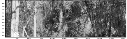
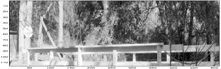
(a)Signal $X^{(1)}.$	(b) Signal $X^{(55)}.$
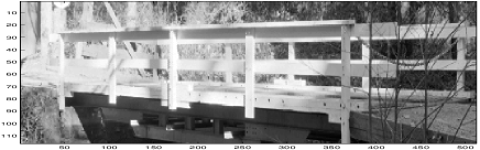
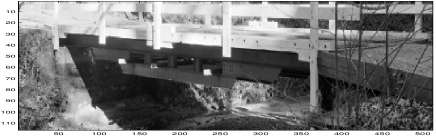
(c) Signal $X^{(115)}.$	(d) Signal $X^{(160)}.$
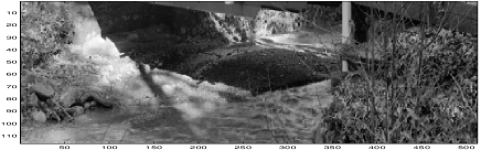
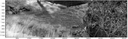
(e) Signal $X^{(225)}.$	(f) Signal $X^{(280)}.$
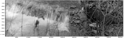
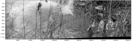
(g) Signal $X^{(340)}.$	(h) Signal $X^{(400)}.$

Figure 1: Examples of selected reference signals.

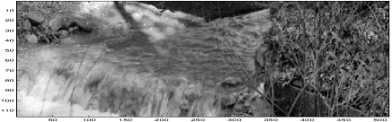
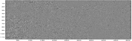
(a)	(b)
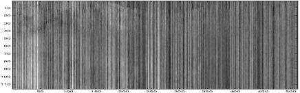
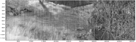
(c)	(d)

Figure 2: Illustration of simulation results from Tables 1 and 2. (a): Reference signal $X^{(280)}.$ (b): Observed data $Y^{(280)}$. (c): Reconstruction of $X^{(280)}$ from $Y^{(280)}$ by KLT with compression ratio $10/116$. (d): Reconstruction of $X^{(280)}$ from $Y^{(280)}$ by proposed transform $F$ with compression ratio $10/116$.

5 Simulations

Here, we consider a case where $K_{{}_{X}}$ and $K_{{}_{Y}}$ (introduced in Section 2.2) are represented by finite signal sets with $N$ members, and illustrate the advantages of the proposed technique over methods based on the KLT approach. In many practical problems (arising, e.g, in a DNA analysis [39]) the number $N$ is quite large, for instance, $N=\mathcal{O}(10^{4})$ [39]. In these simulations, we set $N=400$.

Let us suppose that $\mbox{$\mathbf{y}$}(\tau_{1},\cdot)$, $\mbox{$\mathbf{y}$}(\tau_{2},\cdot)$, $\ldots$, $\mbox{$\mathbf{y}$}(\tau_{400},\cdot)$ are $400$ input stochastic signals where $\mbox{$\mathbf{y}$}(\tau_{k},\cdot)\in L^{2}(\Omega,\mbox{$\mathbb{R}$}^{n})$, for $k=1,\ldots,400$ and $n=116$. Reference stochastic signals are $\mbox{$\mathbf{x}$}(\tau_{1},\cdot),$ $\mbox{$\mathbf{x}$}(\tau_{2},\cdot),\ldots,\mbox{$\mathbf{x}$}(\tau_{{400}},\cdot)$, where $\mbox{$\mathbf{x}$}(\tau_{k},\cdot)\in L^{2}(\Omega,\mbox{$\mathbb{R}$}^{m})$, for $k=1,\ldots,400$ and $m=n=116$. Thus, in these simulations, the interval $[a\hskip 2.84526ptb]$ introduced in Section 2.2 is modelled as 400 points $\tau_{k}$ with $k=1,\ldots,400$ so that $[a\hskip 2.84526ptb]=[\tau_{1},\tau_{2},\ldots,\tau_{{400}}]$.

Signals $\mbox{$\mathbf{x}$}(\tau_{k},\cdot)$ and $\mbox{$\mathbf{y}$}(\tau_{k},\cdot)$ have been simulated as digital images presented by $116\times 512$ matrices $X^{(k)}$ and $Y^{(k)}$, respectively, with $k=1,\ldots,400$. Each column of matrices $X^{(k)}$ and $Y^{(k)}$ represents a realization of signals $\mbox{$\mathbf{x}$}(\tau_{k},\cdot)$ and $\mbox{$\mathbf{y}$}(\tau_{k},\cdot)$, respectively. Each matrix $X^{(k)}$ represents data obtained from a digital photograph ‘Stream and bridge’. Examples of selected images $X^{(k)}$ are shown in Fig. 1.

Observed noisy images $Y^{(1)},\ldots,Y^{(400)}$ have been simulated in the form

$$Y^{(k)}=\mbox{\tt randn}\bullet X^{(k)}\bullet\mbox{\tt rand},$$

for each $k=1,\ldots,400$. Here, $\bullet$ means the Hadamard product, and randn and rand are $116\times 512$ matrices with random entries, and they simulate noise. The entries of randn are normally distributed with mean zero, variance one and standard deviation one. The entries of rand are uniformly distributed in the interval $(0,1)$. A typical example of such noisy images is given in Fig. 2 (b).

We wish to filter and compress the observed data $Y^{(1)}$, …, $Y^{(400)}$ so that their subsequent reconstructions would be close to the reference signals $X^{(1)}$, …, $X^{(400)}$, respectively.

The proposed transform $\cal F$ given by (67)–(68) and (72)–(73), the generic KLT [7] and the transform [9] were applied to this task. To compare their performance, we address three issues as those in Sections 1.1 and 1.4, as follows.

5.1 Large sets of signals

In these simulations, the signal sets are large but finite. Therefore, the known transforms developed for compression of an individual finite random signal-vector can be applied to this case. This issue has been mentioned in Section 1.1 above. Nevertheless the known methods imply difficulties (an insufficient accuracy and excessive computational work) that are discussed below.

5.2 Associated accuracy and compression ratios

5.2.1 Proposed transform $\cal F$

As it has been mentioned in Section 4.8.2, the proposed technique has two degrees of freedom, a number $p$ of interpolation pairs $\{\mbox{$\mathbf{x}$}_{j},\mbox{$\mathbf{y}$}_{j}\}_{j=1}^{p}$ and rank $r_{j}$ of matrix $G_{j}$ (see (12), (2) and (71)). We set $r=r_{j}$ for all $j=1,\ldots,400$.

To demonstrate properties and advantages of the proposed transform $\cal F$, interpolation pairs $\{X_{1},Y_{1}\},\ldots,\{X_{p},Y_{p}\}$ have been chosen in different ways as follows:

$1$st choice:

$p=9$ and interpolation pairs are $\{X_{1},Y_{1}\}$ $=\{X^{(1)},Y^{(1)}\}$, $\{X_{i+1},Y_{i+1}\}$ $=\{X^{50i},Y^{50i}\}$ for $i=1,\ldots,8$;

$2$nd choice:

$p=21$ and interpolation pairs are $\{X_{1},Y_{1}\}$ $=\{X^{(1)},Y^{(1)}\}$, $\{X_{i+1},Y_{i+1}\}$ $=\{X^{20i},Y^{20i}\}$ for $i=1,\ldots,20$;

$3$rd choice:

$p=41$ and interpolation pairs are $\{X_{1},Y_{1}\}$ $=\{X^{(1)},Y^{(1)}\}$, $\{X_{i+1},Y_{i+1}\}$ $=\{X^{10i},Y^{10i})$ for $i=1,\ldots,40$;

$4$th choice:

$p=81$ and interpolation pairs are $\{X_{1},Y_{1}\}$ $=\{X^{(1)},Y^{(1)}\}$, $\{X_{i+1},Y_{i+1}\}$ $=\{X^{5i},Y^{5i}\}$ for $i=1,\ldots,80$;

For $k=1,\ldots,400$, the accuracy associated with compression, filtering of each $Y^{(k)}$ and its subsequent reconstruction by the proposed transform $F$ is represented by

$$\varepsilon_{k}(F)=\|X^{(k)}-{F}[Y^{(k)}]\|^{2}_{F}$$ (74)

and

$$\varepsilon_{\min}(F)=\min_{k=1,\ldots,400}\varepsilon_{k}(F),\hskip 2.84526pt\varepsilon_{\max}(F)=\max_{k=1,\ldots,400}\varepsilon_{k}(F),$$ (75)

In Fig. 2 (d), an example of the restoration of signal $X^{(280)}$ from noisy observed data $Y^{(280)}$ is given. $X^{(280)}$ and $Y^{(280)}$ are typical representatives of signals under consideration. The image in Fig. 2 (d) has been evaluated for $p=9$ as in the $1$st choice above and the compression ratio $10/116$.

Values of $\varepsilon_{\min}(F)$ and $\varepsilon_{\max}(F)$ associated with different choices of the above interpolation pairs are given in Table 1. In the first column, the compression ratios used in the transform $F$ are given. In particular, it follows from Table 1 that the accuracy improves when the number of interpolation pairs increases. This is a confirmation of the statement (54)–(57) of Theorem 3.

5.2.2 Individual KLTs [7]

To each pair $X^{(k)}$, $Y^{(k)}$, an individual KLT $K_{k}$ has been applied, where $k=1,\ldots,400$. Thus, the KLT $K_{k}$ has to be applied 400 times. In Fig. 2 (c), an example of the restoration of signal $X^{(280)}$ by the KLT with the compression ratio $10/116$ is given.

The error associated with compression, filtering of each $Y^{(k)}$ and its subsequent reconstruction by the KLT is represented by

$$\varepsilon(K_{k})=\|X^{(k)}-{K_{k}}[Y^{(k)}]\|^{2}_{F}.$$ (76)

To compare the proposed transform $F$ and the KLT, we denote

$$\Delta_{{\max}}=\max_{k=1,\ldots,400}[\varepsilon(K_{k})/\varepsilon_{k}(F)]$$ (77)

and

$$\Delta_{{\min}}=\min_{k=1,\ldots,400}[\varepsilon(K_{k})/\varepsilon_{k}(F)].$$ (78)

In other words, $\Delta_{{\max}}$ and $\Delta_{{\min}}$ represent maximal and minimal magnitudes of the ratios of the accuracies associated with $F$ and the KLT $K_{k}$. These ratios have been calculated with the same two ranks of $F$ and $K_{k}$, $r=5$ and $r=10$, i.e. with the same two compression ratios of $F$ and $K_{k}$, $c=5/116$ and $c=10/116$.

The results are presented in Table 2. It follows from Table 2 that our transform $F$ provides the substantially better associated accuracy. Depending on the number of interpolation pairs $p$ and compression ratio $c$, the accuracy associated with $F$ is from 4 to 25 times better than that of the KLT.

5.2.3 Generic KLT

[9]. In these simulations, the generic KLT [9] provides the associated accuracy that is worse than that provided by the individual KLTs above.

5.3 Computational work

The proposed transform requires the computation of $p-1$ pseudo-inverse matrices (in (2), with $M_{G_{j}}=\mbox{$\mathbb{O}$}$), $p-1$ SVDs in (38) and $3(p-1)$ matrix multiplications in (2) and (38). In these simulations, $p=9$, $21$, $41$, $81$.

The individual KLTs applied, for $k=1,\ldots,400$, to each pair $\mbox{$\mathbf{x}$}_{k}:=\mbox{$\mathbf{x}$}(\tau_{k},\cdot)$, $\mbox{$\mathbf{y}$}_{k}:=\mbox{$\mathbf{y}$}(\tau_{k},\cdot)$ require the computation of 400 pseudo-inverse matrices $(E_{y_{k}y_{k}}^{1/2})^{{\dagger}}$ and 400 SVDs of matrices $\langle\langle E_{x_{k}y_{k}}(E_{y_{k}y_{k}}^{1/2})^{{\dagger}}\rangle\rangle_{r_{k}}(E_{y_{k}y_{k}}^{1/2})^{{\dagger}}$. Clearly, the KLTs require substantially more computational work than that by the proposed transform.

5.4 Summary of simulation results

The results of the simulations confirm the theoretical results obtained above. In particular,

(i) the accuracy $\displaystyle\mbox{$\varepsilon$}_{{}_{F}}$ associated with the proposed transform $F$ increases when the number $p$ of interpolation pairs increases (Theorem 3),

(ii) the accuracy $\displaystyle\mbox{$\varepsilon$}_{{}_{F}}$ of our transform is from 4 to 25 times better than the accuracy associated with the KLT-like transforms (depending on the number $p$ of interpolation pairs and the compression ratios),

(iii) the proposed transform requires less computational work than that of the KLT-like transforms.

6 Conclusions

The proposed data compression technique is constructed from a combination of the idea of the piece-wise linear function interpolation and the best rank-constrained operator approximation. This device provides the advantages that allow us to

(i) achieve any desired accuracy in the reconstruction of compressed data (Theorem 3),

(ii) find a single transform to compress and then reconstruct any signal from the infinite signal set (Sections 4.2 and 4.3),

(iii) determine the transform in terms of pseudo-inverse matrices so that the transform always exists (Sections 4.2),

(iv) decrease the computational load compared to the related techniques (Section 5.3),

(v) exploit two degrees of freedom (a number of interpolation pairs and compression ratios) to improve the transform performance, and

(vi) use the same initial information (signal samples) as is usually used in the KLT-like transforms.

References

- [1] E. H. W. Meijering, A chronology of interpolation: From ancient astronomy to modern signal and image processing, Proc. IEEE, 90, 3, pp. 319 - 342, 2002.
- [2] L. L. Scharf, The SVD and reduced rank signal processing, Signal Processing, vol. 25, 113 - 133, 1991.
- [3] Y. Yamashita and H. Ogawa, Relative Karhunen-Loéve transform, IEEE Trans. on Signal Processing, vol. 44, pp. 371-378, 1996.
- [4] Y. Hua and W. Q. Liu, Generalized Karhunen-Loève transform, IEEE Signal Processing Letters, vol. 5, pp. 141-143, 1998.
- [5] J. S. Goldstein, I. Reed, and L. L. Scharf, A Multistage Representation of the Wiener Filter Based on Orthogonal Projections, IEEE Trans. on Information Theory, vol. 44, pp. 2943-2959, 1998.
- [6] Y. Hua, M. Nikpour, and P. Stoica, Optimal Reduced-Rank estimation and filtering, IEEE Trans. on Signal Processing, vol. 49, pp. 457-469, 2001.
- [7] A. Torokhti and P. Howlett, Computational Methods for Modelling of Nonlinear Systems, Elsevier, 2007.
- [8] A. Torokhti and P. Howlett, Optimal Transform Formed by a Combination of Nonlinear Operators: The Case of Data Dimensionality Reduction, IEEE Trans. on Signal Processing, 54, No. 4, pp. 1431-1444, 2006.
- [9] A. Torokhti and P. Howlett, Filtering and Compression for Infinite Sets of Stochastic Signals, Signal Processing, 89, pp. 291-304, 2009.
- [10] A. Torokhti and J. Manton, Generic Weighted Filtering of Stochastic Signals, IEEE Trans. on Signal Processing, 57, issue 12, pp. 4675-4685, 2009.
- [11] A. Torokhti and S. Friedland, Towards theory of generic Principal Component Analysis, J. Multivariate Analysis, 100, 4, pp. 661-669, 2009.
- [12] A. Torokhti and S. Miklavcic, Data Compression under Constraints of Causality and Variable Finite Memory, Signal Processing, 90 , Issue 10, pp. 2822-2834, 2010.
- [13] I.T. Jolliffe, “Principal Component Analysis,” Springer Verlag, New York, 1986.
- [14] I. Johnstone, A. Lu, On Consistency and Sparsity for Principal Components Analysis in High Dimensions, J. of the American Statistical Association, 104, 486, pp. 682-693, 2009.
- [15] S. Simoens, O. Munoz-Medina, J. Vidal, and A. Del Coso, Compress-and-Forward Cooperative MIMO Relaying With Full Channel State Information, IEEE Trans. on Signal Processing, 58, No. 2, pp. 781–791, 2010.
- [16] S.-Y.Shung-Yung Lung, Feature extracted from wavelet eigenfunction estimation for text-independent speaker recognition, Pattern Recognition, 37, 7, pp. 1543-1544, 2004.
- [17] M. L. Honig and J. S. Goldstein, Adaptive reduced-rank interference suppression based on multistage Wiener filter, IEEE Trans. on Communications, vol. 50, no. 6, pp. 986–994, 2002.
- [18] A. Basso, D. Cavagnino, V. Pomponiu and A. Vernone, Blind Watermarking of Color Images Using Karhunen-Loève Transform Keying, The Computer Journal, doi: 10.1093/comjnl/bxq052, 2010.
- [19] J. H. Stock and M. W. Watson, Forecasting using principal components from a large number of predictors, Journal of the American Statistical Association, vol. 97, pp. 1167-1179, 2002.
- [20] D. Zhang , Z. Lu, An efficient, high-order perturbation approach for flow in random porous media via Karhunen-Loève and polynomial expansions, J. of Computational Physics, 194, 2, pp. 773-794, 2004.
- [21] C. Schwab, R. Todora, Karhunen-Loève approximation of random fields by generalized fast multipole methods, J. of Computational Physics, 217, 1, pp. 100-122, 2006.
- [22] K.K. Phoon, H.W. Huang and S.T. Quek, Simulation of strongly non-Gaussian processes using Karhunen-Loève expansion, Probabilistic Engineering Mechanics, 20, 2, pp. 188-198, 2005.
- [23] M. Grigoriu, Evaluation of Karhunen-Loève, Spectral, and Sampling Representations for Stochastic Processes, J. Engrg. Mech., 132, 2, pp. 179-189, 2006.
- [24] L. Raptopoulos, M. Dutra, F. Pinto and A. Filho, Alternative approach to modal gait analysis through the Karhunen-Loève decomposition: An application in the sagittal plane, J. of Biomechanics, 39, 15, pp. 2898-2906, 2006.
- [25] L. Jie1, L. Zhangjun, C. Jianbing, Orthogonal expansion of ground motion and PDEM-based seismic response analysis of nonlinear structures, Earthq. Eng. & Eng. Vib. 8, pp. 313-328, 2009.
- [26] B Penna, T. Tillo, E. Magli, G. Olmo, Transform Coding Techniques for Lossy Hyperspectral Data Compression, IEEE Trans. on Geoscience and Remote Sensing, 45, 5, pp. 1408 - 1421, 2007.
- [27] P. Deheuvels, Karhunen-Loève Expansions of Mean-Centered Wiener Processes, Lecture Notes-Monograph Series, Vol. 51, High Dimensional Probability, pp. 62-76, 2006.
- [28] A. Gassem, Goodness-of-fit test for switching diffusion, Statistical Inference for Stochastic Processes, 13, pp. 97 - 123, 2010.
- [29] M. Gastpar, P.L. Dragotti and M. Vetterli, The Distributed Karhunen-Loève Transform, IEEE Trans. on Information Theory, 52 (12), pp. 5177-5196, 2006.
- [30] M. Effros, H. Fen, Suboptimality of the Karhunen-Loève transform for transform coding, IEEE Trans. on Information Theory, 50, 8, pp. 1605 - 1619, 2004.
- [31] Y. Gao, J. Chen, S. Yu, J. Zhou and L.-M. Po, The training of Karhunen-Loève transform matrix and its application for H.264 intra coding, Multimedia Tools & Appl., 41, pp. 111 - 123, 2009.
- [32] H. Houjou, Coarse Graining of Intermolecular Vibrations by a Karhunen-Love Transformation of Atomic Displacement Vectors, J. Chem. Theory Comput., 5 (7), pp. 1814 - 1821, 2009.
- [33] H. Chen, B. Yin, G. Fang, Y. Wang, Comparison of nonlinear and linear PCA on surface wind, surface height, and SST in the South China Sea, Chinese J. of Oceanology and Limnology, 28, 5, pp. 981 - 989, 2010.
- [34] A. Dubey, V. Yadavaa, Multi-objective optimization of Nd: YAG laser cutting of nickel-based superalloy sheet using orthogonal array with principal component analysis, Optics and Lasers in Engineering, 46, 2, pp,124 - 132, 2008.
- [35] G. H. Golub and C. F. van Loan, Matrix Computations, Johns Hopkins University Press, Baltimore, 1996.
- [36] J. Castrillon-Candas, K. Amaratunga, Fast estimation of continuous Karhunen-Loève eigenfunctions using wavelets, IEEE Trans. on Signal Processing, 50, 1, pp. 78 - 86, 2002.
- [37] A. Ben-Israel and T. N. E. Greville, Generalized Inverses: Theory and Applications, John Wiley & Sons, New York, 1974.
- [38] S. Friedland and A. P. Torokhti, Generalized rank-constrained matrix approximations, SIAM J. Matrix Anal. Appl., 29, issue 2, pp. 656 - 659, 2007.
- [39] S. Friedland, A. Niknejad and L. Chihara,A simultaneous reconstruction of missing data in DNA microarrays, Linear Alg. Appl., 416, pp. 8 - 28, 2006.