GCGE: A Package for Solving Large Scale Eigenvalue Problems by Parallel Block Damping Inverse Power Method

Abstract.

We propose an eigensolver and the corresponding package, GCGE, for solving large scale eigenvalue problems. This method is the combination of damping idea, subspace projection method and inverse power method with dynamic shifts. To reduce the dimensions of projection subspaces, a moving mechanism is developed when the number of desired eigenpairs is large. The numerical methods, implementing techniques and the structure of the package are presented. Plenty of numerical results are provided to demonstrate the efficiency, stability and scalability of the concerned eigensolver and the package GCGE for computing many eigenpairs of large symmetric matrices arising from applications.

1. Introduction

A fundamental and challenging task in modern science and engineering is to solve large scale eigenvalue problems. Although high-dimensional eigenvalue problems are ubiquitous in physical sciences, data and imaging sciences, and machine learning, there is no so many classes of eigensolvers as that of linear solvers. Compared with linear equations, there are less efficient numerical methods for solving large scale eigenvalue problems, which poses significant challenges for scientific computing (Bai et al., 2000). In particular, the eigenvalue problems from complicated systems bring strong demand for eigensolvers with good efficiency, stability and scalability at the same time (Fan et al., 2014, 2015; Yu et al., 2018).

The Krylov subspace methods such as Arnoldi and Lanczos methods are always used to design the eigensolvers (Saad, 1992). In order to use explicitly and implicitly restarted techniques for generalized eigenvalue problems, it is necessary to solve the included linear equations exactly to produce upper Hessenberg matrices. But this requirement is always very difficult for large scale sparse matrices with poor conditions. Based on this consideration, LOBPCG is designed based on some types of iteration processes which do not need to solve the included linear equations exactly (Knyazev and Neymeyr, 2003; Knyazev, 2006; Hetmaniuk and Lehoucq, 2006; Knyazev et al., 2007; Duersch et al., 2018). This property makes LOBPCG be reasonable candidate for solving large scale eigenvalue problems on parallel computers. But the subspace generating method and orthogonalization way lead to the unstability of LOBPCG algorithm (Li et al., 2020; Zhang et al., 2020).

The appearance of high performance computers brings new issues for computing plenty of eigenpairs of large scale matrices, which has not so good efficiency and scalability as solving large scale linear equations. Solving eigenvalue problems on high performance computers needs new considerations about the stability and scalability of orthogonalization for plenty of vectors, efficiency and memory costing for computing Rayleigh-Ritz problems. The aim of this paper is to develop a method and the corresponding package for solving symmetric eigenvalue problems. This method is the combination of damping idea, subspace projection method and inverse power method with dynamic shifts. The package GCGE (Generalized Conjugate Gradient Eigensolver) is written by C language and constructed with the way of matrix-free and vector-free. In order to improve the efficiency, stability and scalability, we also introduce new efficient implementing techniques for orthogonalization and computing Rayleigh-Ritz problems. A recursive orthogonalization method with SVD (Singular Value Decomposition) is proposed in order to improve parallel efficiency. In addition, we also provide a moving mechanism to reduce the dimensions of projection subspaces when solving Rayleigh-Ritz problems. The source code can be downloaded from GitHub with the address https://github.com/Materials-Of-Numerical-Algebra/GCGE.

The rest of the paper is organized as follows. In Section 2, we present the concerned algorithm for eigenvalue problems. The implementing techniques are designed in Section 3. In Section 4, plenty of numerical tests are provided to demonstrate the efficiency, stability and scalability of the proposed algorithm and the associated package. Concluding remarks are given in the last section.

2. GCG algorithm

For simplicity, in this paper, we are concerned with the following generalized algebraic eigenvalue problem: Find eigenvalue $\lambda\in\mathbb{R}$ and eigenvector $x\in\mathbb{R}^{N}$ such that

(1) $$Ax=\lambda Bx,$$

where $A$ is $N\times N$ real symmetric matrix and $B$ is $N\times N$ real symmetric positive definite (SPD) matrix.

The generalized conjugate gradient (GCG) algorithm is a type of subspace projection method, which uses the block damping inverse power idea to generate triple blocks $[X,P,W]$, where $X$ saves the current eigenvector approximation, $P$ saves the information from previous iteration step, and $W$ saves vectors from $X$ by the inverse power iteration with some CG steps. We refer to this method as generalized conjugate gradient algorithm since the structure of triple blocks $[X,P,W]$ is similar to that of conjugate gradient method. Assuming that it is desired to compute the smallest numEigen eigenpairs, the corresponding GCG algorithm is defined by Algorithm 1, where numEigen stands for the number of desired eigenpairs.

Algorithm 1 GCG algorithm

1. Choose numEigen vectors to build the block $X$ and two null blocks $P=[\ ]$, $W=[\ ]$.

2. Define $V=[X,P,W]$ and do orthogonalization to $V$ in the sense of inner product deduced by the matrix $B$.

3. Solve the Rayleigh-Ritz problem $(V^{\top}AV)\hat{x}=\hat{x}\Lambda_{x}$ to obtain $\Lambda_{x}$ and $\hat{x}$, then get new approximate eigenvectors $X^{\tt new}=V\hat{x}$.

4. Check the convergence of eigenpair approximations $(\Lambda_{x},X^{\tt new})$. If the smallest numEigen eigenpairs converge, the iteration will stop.

5. Otherwise, compute $P=X^{\tt new}-X(X^{\top}BX^{\tt new})$ and update $X=X^{\tt new}$.

6. Generate $W$ by solving linear equations $(A-\theta B)W=BX(\Lambda_{x}-\theta I)$ by some CG steps with the initial guess $X$, where the shift $\theta$ is selected dynamically.

7. Then go to STEP 2.

The main difference of Algorithm 1 from LOBPCG is the way to generate $W$ and orthogonalization to $V$. The GCG algorithm uses the inverse power method with dynamic shifts to generate $W$. Meanwhile, the full orthogonalization to $V$ is implemented in order to guarantee the numerical stability. In addition, a new type of recursive orthogonalization method with SVD is designed in the next section.

In Step 3 of Algorithm 1, solving Rayleigh-Ritz problem is a sequential process which can not be accelerated by using normal parallel computing. Furthermore, it is well known that the computing time is superlinearly dependent on the number of desired eigenpairs (Saad, 1992). Then in order to accelerate this part, reducing the dimensions of Rayleigh-Ritz problems is a reasonable way. We will compute the desired eigenpairs in batches when the number of desired eigenpairs is large. In each iteration step, the dimensions of $P$ and $W$ are set to be ${\tt numEigen}/5$ or ${\tt numEigen}/10$. Moreover, a moving mechanism is presented for computing large number of desired eigenpairs. These two strategies can further not only reduce the time proportion of the sequential process for solving Rayleigh-Ritz problems but also reduce the amount of memory required by STEP 3. In addition, the Rayleigh-Ritz problem is distributed to multi computing processes and each process only computes a small part of desired eigenpairs. In other words, the Rayleigh-Ritz problem is solved in parallel. More details of implementing techniques will be introduced in Sections 3.2 and 3.3.

In STEP 6 of Algorithm 1, though the matrix $A-\theta B$ may not be SPD, the CG iteration method is adopted for solving the included linear equations due to the warm start $X$ and the shift $\theta$. Please see Section 3.2 for more details. Furthermore, it is suggested to use the algebraic multigrid method as the preconditioner for STEP 6 of Algorithm 1 with the shift $\theta=0.0$, when the concerned matrices are sparse and come from the discretization of partial differential operators by finite element, finite difference or finite volume, etc.

3. Implementing techniques

In this section, we introduce implementing techniques to improve efficiency, scalability and stability for the concerned eigensolver in this paper. Based on the discussion in the previous sections, we focus on the methods for doing the orthogonalization and computing Rayleigh-Ritz problems. A recursive orthogonalization method with SVD and a moving mechanism are presented. In addition, the package GCGE is introduced, which is written by C language and constructed with the way of matrix-free and vector-free.

3.1. Improvements for orthogonalization

This subsection is devoted to introducing the orthogonalization methods which have been supported by GCGE. So far, we have provided modified block orthogonalization method and recursive orthogonalization method with SVD. The criterion for choosing the orthogonalization methods should be based on the number of desired eigenpairs and the scales of the concerned matrices. The aim is to keep the balance among efficiency, stability and scalability.

The modified Gram-Schmidt method (Stewart, 2008) is designed to improve the stability of classical orthogonalization method. The modified block orthogonalization method is the block version of modified Gram-Schmidt method, which can be defined by Algorithm 2. They have the same accuracy and stability, but the modified block orthogonalization method has better efficiency and scalability.

Let us consider the orthogonalization for $X\in\mathbb{R}^{N\times m}$ and assume $m=b\ell$ in Algorithm 2. We divide $X$ into $\ell$ blocks, i.e., $X=[X_{1},X_{2},\cdots,X_{\ell}]$, where $X_{i}\in\mathbb{R}^{N\times b}$, $i=1,\cdots,\ell$. The orthogonalization process is to make $X$ be orthogonal to $X_{0}$ and do orthogonalization for $X$ itself, where $X_{0}\in\mathbb{R}^{N\times m_{0}}$ has already been orthogonalized, i.e., $X_{0}^{\top}BX_{0}=I$.

Firstly, in order to maintain the numerical stability, the process of deflating components in $X_{0}$ from $X$ is repeated until the norm of $X_{0}^{\top}BX$ is small enough. Secondly, the columns of $X$ in blocks of $\ell$ columns are orthogonalized through the modified Gram-Schmidt method. For each $k=1,\cdots,\ell$ in Algorithm 2, when $X_{k}$ is linear dependent, the rearmost vectors of $X$ are copied to the corresponding location. In addition, Algorithm 2 needs $b+1$ global communications in each ${\tt for}$ iteration. In other words, the total number of global communications is

$$(b+1)(\ell-1)+b=m+m/b-1.$$

In fact, in modified block orthogonalization method, we deflate the components in previous orthogonalized vectors successively for all unorthogonalized vectors in each iteration step. This means Algorithm 2 uses block treatment for the unorthogonalized vectors to improve efficiency and scalability without loss of stability. As default, $b$ is set to be $\min(m/4,200)$.

Algorithm 2 Modified block orthogonalization

1:repeat

2:     Compute $X=X-X_{0}(X_{0}^{\top}(BX))$;

3:until the norm of $X_{0}^{\top}(BX)$ is small enough;

4:for  $k=1:\ell$ do

5:     Orthogonalize $X_{k}$ by modified Gram-Schmidt method;

6:     if $k==\ell$ then

7:         break;

8:     end if

9:     repeat

10:         Compute $\begin{bmatrix}R_{k+1}\\ \vdots\\ R_{\ell}\end{bmatrix}=[{X}_{k+1},\cdots,{X}_{\ell}]^{\top}(BX_{k})$;

11:         Compute $[X_{k+1},\cdots,X_{\ell}]=[{X}_{k+1},\cdots,{X}_{\ell}]-{X}_{k}\begin{bmatrix}R_{k+1}\\ \vdots\\ R_{\ell}\end{bmatrix}^{\top}$;

12:     until the norm of $R_{k+1},\cdots,R_{\ell}$ are small enough;

13:end for

In order to improve efficiency and scalability further, we design a type of recursive orthogonalization method with SVD and the corresponding scheme is defined by Algorithm 3. The aim here is to take full use of level-3 BLAS operations. We also find the paper (Yokozawa et al., 2006) has discussed the similar orthogonalization method without SVD. The contribution here is to combine the recursive orthogonalization method and SVD to improve the scalability.

Algorithm 3 ${\tt RecusiveOrthSVD}($X$,{\tt s},{\tt e})$

1:Compute ${\tt length}={\tt e}-{\tt s}+1$;

2:if ${\tt length}\leq c$ then

3:     repeat

4:         Compute $M=X({\tt:~{},s:e})^{\top}BX({\tt:~{},s:e})$;

5:         Compute SVD of $M=Q\Lambda Q^{\top}$;

6:         Compute $X({\tt:~{},s:e})=X({\tt:~{},s:e})Q\Lambda^{-1/2}$;

7:     until the norm of $\Lambda-I$ is small enough;

8:else

9:     ${\tt s1}={\tt s}$; ${\tt e1}={\tt s}+{\tt length}/2-1$;

10:     ${\tt s2}={\tt e1}+1$; ${\tt e2}={\tt e}$;

11:     Call ${\tt RecusiveOrthSVD}(X,{\tt s1},{\tt e1})$;

12:     repeat

13:         Compute $R=(BX({\tt:~{},s1:e1}))^{\top}X({\tt:~{},s2:e2})$;

14:         Compute $X({\tt:~{},s2:e2})=X({\tt:~{},s2:e2})-X({\tt:~{},s1:e1})R$;

15:     until the norm of $R$ are small enough;

16:     Call ${\tt RecusiveOrthSVD}(X,{\tt s2},{\tt e2})$;

17:end if

Let us consider $X\in\mathbb{R}^{N\times m}$ and $m=2^{\eta}$ in Algorithm 3. The orthogonalization of $X$ is completed by calling ${\tt RecusiveOrthSVD}$ recursively. We use $X({\tt:~{},s:e})$ to stand for the s-th column to e-th column of $X$. When ${\tt length}\leq c$, SVD is applied to computing $X$, where $c$ is set to be $\min(m,16)$ as default. In order to maintain the numerical stability, computing $X$ with SVD is repeated until the matrix $\Lambda$ is close to the identity matrix. In general, the above condition is satisfied after two or three iterations. If $M$ has eigenvalues close to zero, i.e., the set of vectors is linearly dependent, the subsequent vectors will be copied to the corresponding location.

If $c=16$ and we compute $X$ with SVD three times when ${\tt length}\leq c$, the total number of global communications is

$$2^{0}+2^{1}+2^{2}+\cdots+2^{\eta-5}+3\times 2^{\eta-4}=\frac{1}{4}m-1,$$

which is much less than the total number of global communications of Algorithm 2.

The recursive orthogonalization method with SVD is recommended and it is the default choice in our package for the orthogonalization to long vectors. In fact, Algorithms 2 and 3 can both reach the required accuracy for all numerical examples in this paper. In the case of solving generalized eigenvalue problems, $B$-orthogonalization should be considered. Algorithm 3 is more efficient than Algorithm 2 in most cases, which will be shown in Section 4.5.

3.2. Computation reduction for Algorithm 1

In this subsection, let us continue considering the whole computation procedure for Algorithm 1. The aim here is to design efficient ways to compute the Rayleigh-Ritz problem in STEP 3 which include

• Orthogonalizing to $V=[X,P,W]$;

• Computing the small scale matrix $\bar{A}=V^{\top}AV$;

• Solving the standard eigenvalue problem $\bar{A}\hat{x}=\hat{x}\Lambda_{x}$.

Except for the moving mechanism shown in Section 3.3 and the inverse power method with dynamic shifts for solving $W$, the techniques here are almost the same as that in (Li et al., 2020; Zhang et al., 2020). But for easier understanding and completeness, we also introduce them here using more concise expressions. In conclusion, the following main optimization techniques are implemented:

• The converged eigenpairs do not participate the subsequent iteration;

• The sizes of $P$ and $W$ are set to be blockSize, which is equal to numEigen/5 as default;

• The shift is selected dynamically when solving $W$;

• The large scale orthogonalization to $V$ is transformed into the small scale orthogonalization to $P$ and a large scale orthogonalization to $W$;

• The submatrix of $\bar{A}$ corresponding to $X$ can be obtained by $\Lambda_{x}$;

• The submatrix of $\bar{A}$ corresponding to $P$ can be computed by multiplication of small scale dense matrices;

• The Rayleigh-Ritz problem $\bar{A}\hat{x}=\hat{x}\Lambda_{x}$ is solved in parallel;

• The moving mechanism is presented to reduce the dimension of $\bar{A}$ further.

According to STEP 2 of Algorithm 1, we decompose $X$ into three parts

$$X=\begin{bmatrix}X_{c},&X_{n},&X_{\widetilde{n}}\end{bmatrix},$$

where $X_{c}$ denotes the converged eigenvectors and $[X_{n},X_{\widetilde{n}}]$ denotes the unconverged ones. The number of vectors in $X_{n}$ is blockSize. Based on the structure of $X$, the block version has the following structure

$$V=\begin{bmatrix}X_{c},&X_{n},&X_{\widetilde{n}},&P,&W\end{bmatrix}$$

with $V^{\top}BV=I$. And the eigenpairs $\Lambda_{x}$ and $\hat{x}$ can be decomposed into the following form

(2) $$\Lambda_{x}=\begin{bmatrix}\Lambda_{c}&O&O\\ O&\Lambda_{n}&O\\ O&O&\Lambda_{\widetilde{n}}\end{bmatrix},\ \hat{x}=\begin{bmatrix}\hat{x}_{c},&\hat{x}_{n},&\hat{x}_{\widetilde{n}}\end{bmatrix},$$

where $\Lambda_{x}$ is the diagonal matrix.

Then in STEP 3 of Algorithm 1, the small scale eigenvalue problem

$$\bar{A}\hat{x}=\hat{x}\Lambda_{x}$$

has the following form

(3) $$\bar{A}\begin{bmatrix}I&O&O\\ O&\hat{x}_{nn}&\hat{x}_{n\widetilde{n}}\\ O&\hat{x}_{\widetilde{n}n}&\hat{x}_{\widetilde{n}\widetilde{n}}\\ O&\hat{x}_{pn}&\hat{x}_{p\widetilde{n}}\\ O&\hat{x}_{wn}&\hat{x}_{w\widetilde{n}}\\ \end{bmatrix}=\begin{bmatrix}I&O&O\\ O&\hat{x}_{nn}&\hat{x}_{n\widetilde{n}}\\ O&\hat{x}_{\widetilde{n}n}&\hat{x}_{\widetilde{n}\widetilde{n}}\\ O&\hat{x}_{pn}&\hat{x}_{p\widetilde{n}}\\ O&\hat{x}_{wn}&\hat{x}_{w\widetilde{n}}\\ \end{bmatrix}\begin{bmatrix}\Lambda_{c}&O&O\\ O&\Lambda_{n}&O\\ O&O&\Lambda_{\widetilde{n}}\end{bmatrix},$$

where $\bar{A}=V^{\top}AV$, $\hat{x}^{\top}\hat{x}=I$ and $\hat{x}_{c}$, $\hat{x}_{n}$, $\hat{x}_{\widetilde{n}}$ have following structures

(4) $$\hat{x}_{c}=\begin{bmatrix}I\\ O\\ O\\ O\\ O\end{bmatrix},\ \hat{x}_{n}=\begin{bmatrix}O\\ \hat{x}_{nn}\\ \hat{x}_{\widetilde{n}n}\\ \hat{x}_{pn}\\ \hat{x}_{wn}\end{bmatrix},\ \hat{x}_{\widetilde{n}}=\begin{bmatrix}O\\ \hat{x}_{n\widetilde{n}}\\ \hat{x}_{\widetilde{n}\widetilde{n}}\\ \hat{x}_{p\widetilde{n}}\\ \hat{x}_{w\widetilde{n}}\end{bmatrix}.$$

In addition, Ritz vectors is updated as

$$X^{\tt new}=V\hat{x}.$$

In STEP 4 of Algorithm 1, the convergence of the eigenpairs $(\Lambda_{x},X^{\tt new})$ is checked. Due to (2), we set

$$\hat{x}_{n}=\begin{bmatrix}\hat{x}_{n_{1},}&\hat{x}_{n_{2}}\end{bmatrix},\ \hat{x}_{\widetilde{n}}=\begin{bmatrix}\hat{x}_{\widetilde{n}_{1}},&\hat{x}_{\widetilde{n}_{2}}\end{bmatrix},$$

$$\Lambda_{n}=\begin{bmatrix}\Lambda_{n_{1}}&O\\ O&\Lambda_{n_{2}}\end{bmatrix},\ \Lambda_{\widetilde{n}}=\begin{bmatrix}\Lambda_{\widetilde{n}_{1}}&O\\ O&\Lambda_{\widetilde{n}_{2}}\end{bmatrix},$$

and the diagonal of $\Lambda_{n_{1}}$ inclues the new converged eigenvalues. Then all $\ell$ convergened eigenvectors are in

$$X^{\tt{new}}_{c}=V\begin{bmatrix}\hat{x}_{c},&\hat{x}_{n_{1}}\end{bmatrix},\$$

and the unconverged ones are in

$$X^{\tt{new}}_{n}=V\begin{bmatrix}\hat{x}_{n_{2}},&\hat{x}_{\widetilde{n}_{1}}\end{bmatrix}\mbox{ and }\ X^{\tt{new}}_{\widetilde{n}}=V\hat{x}_{\widetilde{n}_{2}}.$$

If $\ell$ is equal to numEigen, the iteration will stop. Otherwise, $0\leq\ell<{\tt numEigen}$ and the iteration will continue. Here, the length of $X^{\tt{new}}_{n}$ is

$${\tt blockSize}=\min({\tt numEigen/5},{\tt numEigen}-\ell).$$

In STEP 5 of Algorithm 1, in order to produce $P$ for the next GCG iteration, from the definition of $\hat{x}_{n}$ in (4) and the orthonormality of $V$, i.e., $V^{\top}BV=I$, we first set

$$\widetilde{P}=V\hat{x}_{n}-X_{n}(X_{n}^{\top}BV\hat{x}_{n})=V\widetilde{p},$$

where

(5) $$\widetilde{p}=\begin{bmatrix}O\\ O\\ \hat{x}_{\widetilde{n}{n}}\\ \hat{x}_{pn}\\ \hat{x}_{wn}\end{bmatrix}.$$

In order to compute $P^{\tt new}$ to satisfy $(X^{\tt new})^{\top}BP^{\tt new}=O$, we come to do the orthogonalization for small scale vectors in $[\hat{x},\widetilde{p}]$ according to the $L^{2}$ inner product. Since vectors in $\hat{x}$ are already orthonormal, the orthogonalization only needs to be done for $\widetilde{p}$ against $\hat{x}$ to get a new vectors $\hat{p}$. Thus let $[\hat{x},\hat{p}]$ denote the orthogonalized block, i.e.,

(6) $$\begin{bmatrix}\hat{x},&\hat{p}\end{bmatrix}^{\top}\begin{bmatrix}\hat{x},&\hat{p}\end{bmatrix}=I.$$

Then,

$$P^{\tt{new}}=V\hat{p}.$$

Moreover, it is easy to check that

$$(X^{\tt{new}})^{\top}BP^{\tt{new}}=\hat{x}^{\top}V^{\top}BV\hat{p}=O$$

and

$$(P^{\tt{new}})^{\top}BP^{\tt{new}}=\hat{p}^{\top}V^{\top}BV\hat{p}=I.$$

In STEP 6 of Algorithm 1, $\widetilde{W}$ is obtained by some CG iterations for the linear equations

(7) $$(A-\theta B)\widetilde{W}=BX^{\tt{new}}_{n}\begin{bmatrix}\Lambda_{n_{2}}-\theta I&O\\ O&\Lambda_{\widetilde{n}_{1}}-\theta I\end{bmatrix}$$

with the initial guess $X^{\tt{new}}_{n}$, where the shift $\theta$ is set to be the largest converged eigenvalue in the convergence process. It is noted that the shift is not fixed and the matrix $A-\theta B$ may not be SPD, but the initial guess $X^{\tt{new}}_{n}$ is perpendicular to the eigenvectors of $A-\theta B$ corresponding to all negtive eigenvalues, i.e.,

$$(X^{\tt{new}}_{n})^{\top}(A-\theta B)X^{\tt{new}}_{c}=O,$$

since $X^{\tt{new}}_{c}$ reaches the convergence criterion. In other words, $A-\theta B$ is SPD in the orthogonal complement space of $\mbox{span}(X^{\tt{new}}_{c})$. Then the CG iteration method can be adopted for solving the included linear equations. Due to the shift $\theta$, the multiplication of matrix and vector of each CG iteration takes more time, but the convergence of GCG algorithm is accelerated. In addition, there is no need to solve linear equations (7) with high accuracy, and only $10$-$30$ CG iterations are enough during each GCG iteration. In Remark 3.1, an example is presented to explain why the convergence of GCG algorithm with dynamic shifts is accelerated after one CG iteration. In Section 4.1, we give some numerical results to show the performance of GCGE with dynamic shifts and the convergence procedure under different number of CG iterations. In order to produce $W^{\tt{new}}$ for the next GCG iteration, using Algorithm 3, we need to do the orthognalization to $\widetilde{W}$ according to $[X^{\tt{new}},P^{\tt{new}}]$, i.e.,

$$\begin{bmatrix}X^{\tt{new}},&P^{\tt{new}}\end{bmatrix}^{\top}BW^{\tt{new}}=O,\ (W^{\tt{new}})^{\top}BW^{\tt{new}}=I.$$

Remark 3.1.

We give an example to present the accelerating convergence of GCG algorithm with dynamic shifts after one CG iteration. Assuming that the first eigenpair $(\lambda_{1},v_{1})$ has been found for the standard eigenvalue problem

$$Ax=\lambda x,$$

we have the approximate eigenvector $x_{0}=a_{2}v_{2}+a_{3}v_{3}$ of the second eigenvector, where

$$Av_{2}=\lambda_{2}v_{2},\ Av_{3}=\lambda_{3}v_{3},\mbox{ and }\ 0<\lambda_{1}<\lambda_{2}\leq\lambda_{3}.$$

For the linear equations

$$(A-\theta I)w=(\tilde{\lambda}-\theta)x_{0}\mbox{ and }\ 0\leq\theta<\lambda_{2},$$

we can obtain the new approximate eigenvector

$$x_{1}=\frac{a_{2}^{2}+a_{3}^{2}}{a_{3}^{2}(\lambda_{2}-\theta)+a_{2}^{2}(\lambda_{3}-\theta)}\Big{(}(\lambda_{3}-\theta)a_{2}v_{2}+(\lambda_{2}-\theta)a_{3}v_{3}\Big{)},$$

after the first CG iteration with the initial guess $x_{0}$, where $\tilde{\lambda}=x_{0}^{\top}Ax_{0}/x_{0}^{\top}x_{0}$. It is noted that the convergence rate is

$$\frac{\lambda_{2}-\theta}{\lambda_{3}-\theta},$$

which is less than the case of $\theta=0$.

Backing to STEP 2 of Algorithm 1, we denote

$$V^{\tt{new}}=\begin{bmatrix}X^{\tt{new}},&P^{\tt{new}},&W^{\tt{new}}\end{bmatrix}=\begin{bmatrix}V\hat{x},&V\hat{p},&W^{\tt{new}}\end{bmatrix}.$$

During solving the Rayleigh-Ritz problem, we need to assemble the small scale matrices $(V^{\tt{new}})^{\top}AV^{\tt{new}}$ and $(V^{\tt{new}})^{\top}BV^{\tt{new}}$. Since the orthogonalization to the vectors in $V^{\tt{new}}$ has been done by the inner product deduced by the matrix $B$, $(V^{\tt{new}})^{\top}BV^{\tt{new}}$ is an identity matrix. Then we only need to compute the matrix $\bar{A}_{\tt new}$, which is equal to

(8) $$\begin{bmatrix}(X^{\tt{new}})^{\top}AX^{\tt{new}}&(X^{\tt{new}})^{\top}AP^{\tt{new}}&(X^{\tt{new}})^{\top}AW^{\tt{new}}\\ (P^{\tt{new}})^{\top}AX^{\tt{new}}&(P^{\tt{new}})^{\top}AP^{\tt{new}}&(P^{\tt{new}})^{\top}AW^{\tt{new}}\\ (W^{\tt{new}})^{\top}AX^{\tt{new}}&(W^{\tt{new}})^{\top}AP^{\tt{new}}&(W^{\tt{new}})^{\top}AW^{\tt{new}}\end{bmatrix}.$$

From (3), the submatrix $(X^{\tt{new}})^{\top}AX^{\tt{new}}$ does not need to be computed explicitly since it satisfies the following formula

(9) $$(X^{\tt{new}})^{\top}AX^{\tt{new}}=\hat{x}^{\top}V^{\top}AV\hat{x}=\hat{x}^{\top}\bar{A}\hat{x}=\Lambda_{x}.$$

Based on the basis in $V$ and (6), we have

(10) $$(P^{\tt{new}})^{\top}AP^{\tt{new}}=\hat{p}^{\top}V^{\top}AV\hat{p}=\hat{p}^{\top}\bar{A}\hat{p}$$

and

(11) $$(P^{\tt{new}})^{\top}AX^{\tt{new}}=\hat{p}^{\top}V^{\top}AV\hat{x}=\hat{p}^{\top}\bar{A}\hat{x}=\hat{p}^{\top}\hat{x}\Lambda_{x}=O.$$

Thus from (8), (9), (10) and (11), we know the matrix $\bar{A}^{\tt{new}}$ has the following structure

(12) $$\begin{bmatrix}\Lambda_{0}&O&O&O\\ O&\Lambda_{1}&O&\alpha_{1}\\ O&O&\alpha_{0}&\alpha_{2}\\ O&\alpha_{1}^{\top}&\alpha_{2}^{\top}&\alpha_{3}\\ \end{bmatrix},$$

where

$$\Lambda_{0}=\begin{bmatrix}\Lambda_{c}&O\\ O&\Lambda_{n_{1}}\end{bmatrix},\ \Lambda_{1}=\begin{bmatrix}\Lambda_{n_{2}}&O&O\\ O&\Lambda_{\widetilde{n}_{1}}&O\\ O&O&\Lambda_{\widetilde{n}_{2}}\end{bmatrix},$$

$$\alpha_{0}=\hat{p}^{\top}\bar{A}\hat{p},\ \alpha_{1}=\begin{bmatrix}X^{\tt new}_{n},&X^{\tt{new}}_{\widetilde{n}}\end{bmatrix}^{\top}AW^{\tt{new}},$$

$$\alpha_{2}=(P^{\tt{new}})^{\top}AW^{\tt{new}},\ \alpha_{3}=(W^{\tt{new}})^{\top}AW^{\tt{new}}.$$

It is noted that since $X^{\tt new}_{c}$ reaches the convergence criterion, we assume the equation

$$AX^{\tt new}_{c}=BX^{\tt new}_{c}\Lambda^{\tt new}_{c}$$

is satisfied. Then

$$(W^{\tt new})^{\top}AX^{\tt new}_{c}=(W^{\tt new})^{\top}BX_{c}^{\tt new}\Lambda^{\tt new}_{c}=O$$

is satisfied approximately since $(W^{\tt new})^{\top}BX^{\tt new}_{c}=O$.

After assembling matrix $\bar{A}^{\tt new}$, the next task is to solve the new small scale eigenvalue problem:

(13) $$\bar{A}^{\tt{new}}\hat{x}^{\tt{new}}=\hat{x}^{\tt{new}}\Lambda_{x}^{\tt{new}},$$

in STEP 3. Due to the converged eigenvectors $X^{\tt new}_{c}$ in $V^{\tt new}$, there are already $\ell$ converged eigenvectors of $\bar{A}^{\tt{new}}$ and they all have the form

$$(0,...,0,1,0,...0)^{\top}$$

($1$ stays in the position of associated converged eigenvalue). We only need to compute the unconverged eigenpairs corresponding to $[X^{\tt new}_{n},X^{\tt new}_{\widetilde{n}}]$ for the eigenvalue problem (13). The subroutine dsyevx from LAPACK (Anderson et al., 1999) is called to compute the only $(\ell+1)$-th to ${\tt numEigen}$-th eigenvalues and their associated eigenvectors.

In order to reduce time consuming of this part, this task is distributed to multi computing processes and each process only computes a small part of desired eigenpairs. After all processes finish their tasks, the subroutine ${\tt MPI\_Allgatherv}$ is adopted to gather all eigenpairs from all processes and deliver them to all. This way leads to an obvious time reduction for computing the desired eigenpairs of (13). Since more processes lead to more communicating time, we choose the number of used processes for solving (13) such that each process computes at least $10$ eigenpairs.

Remark 3.2.

In order to accelerate the convergence, the size of $X$, sizeX, is always chosen to be greater than numEigen, which is set to be the minimum of ${\tt numEigen}+3\times{\tt blockSize}$ and the dimension of $A$, as default.

Remark 3.3.

Since the converged eigenpairs $(\Lambda_{c},X_{c})$ do not participate in the subsequent iterations, in real implementation, $\bar{A}$ is computed as follows

$$\begin{bmatrix}X_{n},&X_{\widetilde{n}},&P,&W\end{bmatrix}^{\top}A\begin{bmatrix}X_{n},&X_{\widetilde{n}},&P,&W\end{bmatrix},$$

and the corresponding eigenpairs have the forms

$$\begin{bmatrix}\Lambda_{n}&O\\ O&\Lambda_{\widetilde{n}}\end{bmatrix},\ \begin{bmatrix}\hat{x}_{nn}&\hat{x}_{n\widetilde{n}}\\ \hat{x}_{\widetilde{n}n}&\hat{x}_{\widetilde{n}\widetilde{n}}\\ \hat{x}_{pn}&\hat{x}_{p\widetilde{n}}\\ \hat{x}_{wn}&\hat{x}_{w\widetilde{n}}\end{bmatrix}.$$

In other words, the internal locking (deflation) is implemented to prevent computing over again the eigenpairs which have been found.

3.3. The moving mechanism

In Algorithm 1, the small scale eigenvalue problem (13) needs to be solved, in which the dimension of the dense matrix $\bar{A}$ is

$${\tt sizeX}+2\times{\tt blockSize},$$

where the size of $X$, sizeX, is equal to ${\tt numEigen}+3\times{\tt blockSize}$. When numEigen is large, e.g., $5000$, with ${\tt blockSize}=200$, dsyevx should be called to solve $5000$ eigenpairs for a dense matrix of $6000$-dimension. In this case, the time of STEP 3 of Algorithm 1 is always dominated.

In order to improve efficiency further for the above case, we present a moving mechanism. Firstly, the maximum project dimension is set to be ${\tt maxProjDim}=5\times{\tt blockSize}$ in moving procedure, i.e., the size of $X$ is set to be $3\times{\tt blockSize}$ and the sizes of $P$ and $W$ are both ${\tt blockSize}$. Secondly, when $2\times{\tt blockSize}$ eigenpairs converged, all the eigenpairs of $\bar{A}$ will be solved, i.e, $\bar{A}$ is decomposed into

$$\bar{A}=\begin{bmatrix}\hat{x},&\hat{p},&\hat{w}\end{bmatrix}\Lambda_{xpw}\begin{bmatrix}\hat{x},&\hat{p},&\hat{w}\end{bmatrix}^{-1},$$

where

$$\bar{A}=V^{\top}AV,\ V=\begin{bmatrix}X,&P,&W\end{bmatrix}.$$

In addition, the new $X$ is equal to $V[\hat{x},\hat{p},\hat{w}]$, and $\Lambda_{xpw}$ can be used to construct the new $\bar{A}$ in the next STEP 3. In other words, $P$ and $W$ have been integrated into $X$. Then, the new $P$ and $W$ will be computed and stored behind the new $X$. When there are new converged $2\times{\tt blockSize}$ eigenpairs again, $P$ and $W$ will be integrated into $X$ again, and so on. The above process is shown in Figure 1. It is noted that the dimension of the dense matrix $\bar{A}$ is ${\tt maxProjDim}=5\times{\tt blockSize}$ at most in the small scale eigenvalue problem (13).

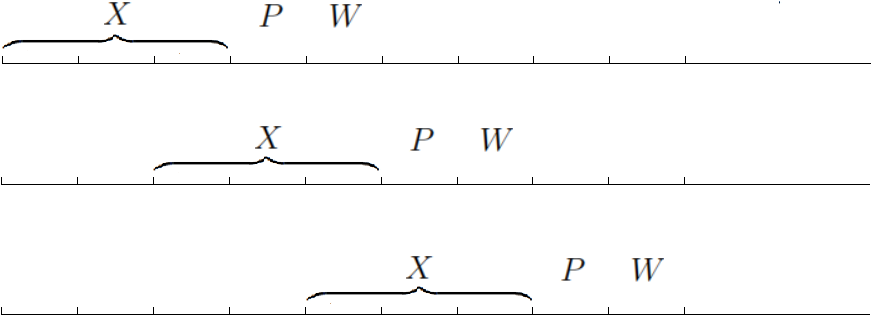
Figure 1. Moving $[X,P,W]$, when $2\times{\tt blockSize}$ eigenpairs converged.

Moving $[X,P,W]$, when $2\times{\tt blockSize}$ eigenpairs converged.

Moreover, the moving mechanism can greatly reduce memory requirements, which allows more eigenpairs to be computed. Specifically speaking, the double array, of which the size is

(14) $$\begin{split}&({\tt sizeX}+2\times{\tt blockSize})+2\times({\tt maxProjDim})^{2}\\ &+10\times({\tt maxProjDim})+{\tt sizeX}\times{\tt blockSize},\end{split}$$

is required to be stored in each process. The first two terms denote the sizes of the two arrays which are used to store the eigenpairs and the dense matrix in the small scale eigenvalue problem (13). The third term is the size of workspace for dsyevx. The last term is the size of the array which is used in STEP 5. In Figure 2, the required memory computed by (14) is shown with and without the moving mechanism.

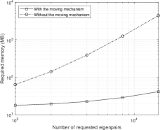
Figure 2. Requested memory in each process

3.4. Matrix-free and vector-free operations

Based on Algorithm 1 and its implementing techniques presented in above sections, we develop the package GCGE, which is written by C language and constructed with the way of matrix-free and vector-free. So far, the package has included the eigensolvers for the matrices which are stored in dense format, compressed row/column sparse format or are supported in MATLAB, Hypre (Falgout et al., 2006), PETSc (Balay et al., 1997), PHG (Zhang, 2009) and SLEPc (Hernandez et al., 2005). Table 1 presents the currently supported matrix-vector structure. It is noted that there is no need to copy the built-in matrices and the vectors from these softwares/libraries to the GCGE package.

Table 1. Supported matrix-vector structures

	matrix structure name	vector structure name
MATLAB	sparse distributed matrix	full stored matrix
Hypre	hypre_ParCSRMatrix	hypre_ParVector
PETSc	Mat	Vec
PHG	MAT	VEC
SLEPc	Mat	BV

A user can also build his own eigensolver by providing the matrix, vector structures and their operations. The following six matrix-vector operations should be provided by the user:

• VecCreateByMat

• VecDestroy

• VecLocalInnerProd

• VecSetRandomValue

• VecAxpby

• MatDotVec

They realize creating and destroying vector according to matrix, computing local inner product of vectors $x$ and $y$, setting random values for vector $x$, computing vector $y=\alpha x+\beta y$, computing vector $y=Ax$, respectively. VecInnerProd, i.e., computing inner product of vectors $x$ and $y$, has been provided through calling VecLocalInnerProd and MPI_Allreduce.

The default matrix-multi-vector operations are invoked based on the above matrix-vector operations and the additional two operations: GetVecFromMultiVec and RestoreVecForMultiVec, which are getting/restoring one vector from/to multi vectors. For higher efficiency, it is strongly recommended that users should provide the following six matrix-multi-vector operations:

• MultiVecCreateByMat

• MultiVecDestroy

• MultiVecLocalInnerProd

• MultiVecSetRandomValue

• MultiVecAxpby

• MatDotMultiVec

In addition, if user-defined multi-vector is stored in dense format, BLAS library can be used to implement (1)-(5) operators easily, which has been provided in the GCGE package. In other words, only one operator, i.e., computing the multiplication of matrix and multi-vector needs to be provided by users.

In order to improve the parallel efficiency of computing inner products of multi-vector $X$ and $Y$, i.e., the operation MultiVecInnerProd, a new MPI data type with the corresponding reduced operation has been created by

            MPI_Type_vector, MPI_Op_create.

The variable MPI_IN_PLACE is used as the value of sendbuf in MPI_Allreduce at all processes.

Although SLEPc (Hernandez et al., 2005) provides an inner product operation for BV structure, we still recommend using our own multi-vector inner product operation. Let us give an example to illustrate the reason. For instance, we need to compute the inner products

$$[x_{i},\cdots,x_{j}]^{\top}[y_{p},\cdots,y_{q}]$$

and the results are stored in the following submatrix

(15) $$\begin{bmatrix}c_{ip}&\cdots&c_{iq}\\ \vdots&&\vdots\\ c_{jp}&\cdots&c_{jq}\end{bmatrix}.$$

Always, the vectors $[x_{i},\cdots,x_{j}]$ and $[y_{p},\cdots,y_{q}]$ come from the multi-vector

$$X =[x_{1},\cdots,x_{i},\cdots,x_{j},\cdots,x_{n}],$$

$$Y =[y_{1},\cdots,y_{p},\cdots,y_{q},\cdots,y_{m}].$$

and the dense matrix (15) is one submatrix of the following matrix

$$\begin{bmatrix}*&*&\cdots&*&*\\ *&c_{ip}&\cdots&c_{iq}&*\\ *&\vdots&&\vdots&*\\ *&c_{jp}&\cdots&c_{jq}&*\\ *&*&\cdots&*&*\end{bmatrix}_{s\times t}$$

which is stored by column. Thus, it can be noted that the above mentioned submatrix (15) is not stored continuously.

The result of the SLEPc’s inner product operation, BVDot, must be stored in a sequential dense matrix with dimensions $n\times m$ at least. In other words, regardless of the values of $i$, $j$, $p$ and $q$, in each process, the additional memory space is required, of which the size is $n\times m$. In general, $n$ and $m$ are set to be ${\tt sizeX}+2\times{\tt blockSize}$ in the GCG algorithm, while $s$ and $t$ are much less than $n$ and $m$, respectively.

In the GCGE package, the operation MultiVecInnerProd is implemented as follows:

• Through MultiVecLocalInnerProd, local inner products are calculated and stored in the above mentioned submatrix for each process;

• A new MPI_Datatype named SUBMAT is created by

  int MPI_Type_vector(
      int count, int length, int stride,
      MPI_Datatype oldtype, MPI_Datatype *newtype)
  

  with

      count=q-p+1, length=j-i+1, stride=s;
  

• Through MPI_Op_create, the operation of sum of SUBMAT is created, which is named as SUM_SUBMAT;

• Then

  int MPI_Allreduce(
      void *sendbuf, void *recvbuf, int count,
      MPI_Datatype datatype, MPI_Op op,
      MPI_Comm comm)
  

  is called with

          sendbuf=MPI_IN_PLACE, count=1,
          datatype=SUBMAT, op=SUM_SUBMAT
  

  to gather values from all processes and distribute the results back to all processes.

Obviously, no extra workspace is needed here. The memory requirements are reduced for each process.

4. Numerical results

The numerical experiments in this section are carried out on LSSC-IV in the State Key Laboratory of Scientific and Engineering Computing, Chinese Academy of Sciences. Each computing node has two 18-core Intel Xeon Gold 6140 processors at 2.3 GHz and 192 GB memory. For more information, please check http://lsec.cc.ac.cn/chinese/lsec/LSSC-IVintroduction.pdf. We use numProc to denote the number of processes in numerical experiments.

In this section, the GCG algorithm defined by Algorithm 1 and the implementing techniques in Section 3 are investigated for thirteen standard eigenvalue problems and one generalized eigenvalue problem. The first thirteen matrices are available in Suite Sparse Matrix Collection, which have clustered eigenvalues and many negative eigenvalues. The first matrix named Andrews is provided by Stuart Andrews at Brown University, which has seemingly random sparsity pattern. The second to the thirteenth matrices are generated by the pseudo-potential algorithm for real-space electronic structure calculations (Kronik et al., 2006; Natan et al., 2008; Saad et al., 2010). The FEM matrices $A$ and $B$ come from the finite element discretization for the following Laplace eigenvalue problem: Find $(\lambda,u)\in\mathbb{R}\times H_{0}^{1}(\Omega)$ such that

(18) $$\left\{\begin{array}[]{rcl}-\Delta u&=&\lambda u,\ \ \ \ {\rm in}\ \Omega,\\ u&=&0,\ \ \ \ \ \ {\rm on}\ \partial\Omega,\end{array}\right.$$

where $\Omega=(0,1)\times(0,1)\times(0,1)$. The discretization of the eigenvalue problem (18) by the conforming cubic finite element (P3 element) with 3,145,728 elements leads to the stiffness matrix $A$ and the mass matrix $B$. The concerned matrices are listed in Table 2, where the density is defined by

$$\frac{\mbox{the number of non-zero entries}}{\mbox{dimension}\times\mbox{dimension}}.$$

The proposed GCG algorithm given by Algorithm 1 based on BV structure from SLEPc is adopted to solve eigenpairs of the concerned matrices in Table 2.

Table 2. Testing matrices

ID	Matrix	Dimension	Non-zero Entries	Density
1	Andrews	60,000	760,154	2.11e-4
2	CO	221,119	7,666,057	1.57e-4
3	Ga10As10H30	113,081	6,115,633	4.78e-4
4	Ga19As19H42	133,123	8,884,839	5.01e-4
5	Ga3As3H12	61,349	5,970,947	1.59e-3
6	Ga41As41H72	268,096	18,488,476	2.57e-4
7	Ge87H76	112,985	7,892,195	6.18e-4
8	Ge99H100	112,985	8,451,395	6.62e-4
9	Si34H36	97,569	5,156,379	5.42e-4
10	Si41Ge41H72	185,639	15,011,265	4.36e-4
11	Si5H12	19,896	738,598	1.87e-3
12	Si87H76	240,369	10,661,631	1.85e-4
13	SiO2	155,331	11,283,503	4.68e-4
14	FEM matrices $A$ and $B$	14,045,759	671,028,055	3.40e-6

The convergence criterion is set to be

$$\|Ax-\lambda x\|_{2}/\|x\|_{2}<{\tt tol}$$

for the first thirteen matrices and

$$\|Ax-\lambda Bx\|_{2}/(\lambda\|B^{1/2}x\|_{2})<{\tt tol}$$

for FEM matrices, where the tolerance, tol, is set to be $10^{-8}$ as default. Moreover, we set ${\tt blockSize}={\tt numEigen}/10$ for the first thirteen matrices and ${\tt blockSize}={\tt numEigen}/5$ for FEM matrices.

In order to confirm the efficiency, stability and scalability of GCGE, we investigate the numerical comparison between GCGE and LOBPCG. We will find that GCGE has better efficiency, stability than LOBPCG and they have almost the same scalability. In addition, Krylov-Schur method is also compared in Sections 4.2 and 4.5.

4.1. About dynamic shifts and the number of CG iterations

In this subsection, we give some numerical results to show the performance of GCGE with dynamic shifts and the convergence procedure under different number of CG iterations.

In STEP 6 of Algorithm 1, the linear equations (7) are solved by some CG iterations. Due to the shift $\theta$, the multiplication of matrix and vector of each CG iteration takes more time, but the convergence of GCG algorithm is accelerated. For the standard eigenvalue problems, i.e., $B=I$, because the additional computation is only the linear operations on vectors, each GCG iteration with dynamic shifts takes a little more time than the case of no shift. As shown in Figure 3, the performance of GCGE with dynamic shifts is greatly improved. In addition, the total number of GCG iterations is presented in Table 3.

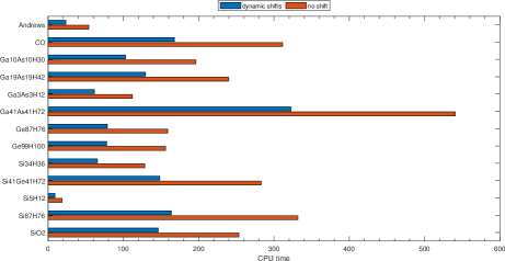
Figure 3. ${\tt tol}=10^{-8}$, ${\tt numEigen}=800$, and ${\tt numProc}=36$

Table 3. The total number of GCG iterations

ID	Matrix	Dynamic Shifts	No Shift	Ratio
1	Andrews	102	281	36.29%
2	CO	97	195	49.74%
3	Ga10As10H30	105	213	49.29%
4	Ga19As19H42	110	216	50.92%
5	Ga3As3H12	81	165	49.09%
6	Ga41As41H72	133	236	56.35%
7	Ge87H76	78	212	36.79%
8	Ge99H100	77	206	37.37%
9	Si34H36	79	207	38.16%
10	Si41Ge41H72	87	208	41.82%
11	Si5H12	86	201	42.78%
12	Si87H76	89	232	38.36%
13	SiO2	90	164	54.87%

For the generalized eigenvalue problems, there is no significant improvement for the overall performance of GCGE with dynamic shifts by the additional computation of the multiplication of matrix $B$ and vectors. When the matrix $A$ can be modified, we recommend users to generate $A-\theta B$ explicitly and do CG steps for $A-\theta B$ directly. In this event, GCGE with dynamic shifts will perform better for the generalized eigenvalue problem and the results for ${\tt numEigen}=800$ and numEigen = 5000 are shown in Tables 4 and 7 respectively.

Table 4. FEM matrices with ${\tt numEigen}=800$, ${\tt tol}=10^{-12}$ and ${\tt numProc}=576$

	The Total Number	CPU Time (in seconds)
	of GCG Iterations
Dynamic Shifts	83	1669.19
No Shift	88	1777.87
Ratio	94.31%	93.88%

In addition, the GCG algorithm do not need to solve linear equations exactly in STEP 6. In the rest of this subsection, the total time of GCGE and the average time per each GCG iteration are presented under different number of CG iterations. Because the first thirteen matrices have similar density, we choose SiO2 with ${\tt numProc}=36$ and FEM matrices with ${\tt numProc}=576$ as test objects.

For SiO2 with ${\tt numEigen}=400$ and $800$, as shown in Figures 4 and 5, when the number of CG iterations is increased from $5$ to $35$ in each GCG iteration, the number of GCG iterations decreases and the average time per each GCG iteration increases. And the total time reaches a minimum near $15$ CG iterations according to Figure 6. In fact, from Andrews to SiO2, there have similar conclusions.

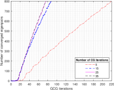
Figure 4. Convergence procedure for SiO2 with ${\tt tol}=10^{-8}$

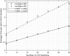
Figure 5. Average time for SiO2 with ${\tt tol}=10^{-8}$

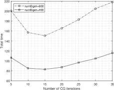
Figure 6. Total time for SiO2 with ${\tt tol}=10^{-8}$

Figures 7 and 8 show the corresponding results for FEM matrices with ${\tt numEigen}=100$ and $200$. When the number of CG iterations is increased from $10$ to $70$, the number of GCG iterations decreases and the average time per each GCG iteration increases. The best performance is achieved at $30$-$40$ CG iterations as shown in Figure 9.

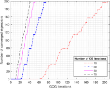
Figure 7. Convergence procedure for FEM matrices with ${\tt tol}=10^{-8}$

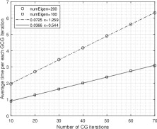
Figure 8. Average time for FEM matrices with ${\tt tol}=10^{-8}$

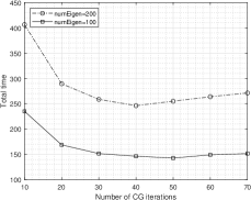
Figure 9. Total time for FEM matrices with ${\tt tol}=10^{-8}$

It is noted that the number of CG iterations in each GCG iteration affects the efficiency of the algorithm deeply as presented in Figures 5 and 8. The average time per each GCG iteration is linearly associated with the number of CG iterations. So, the number of CG iterations is a key parameter for trading off between the number of GCG iterations and the average time of GCG iterations. In fact, the total time of GCG algorithm is nearly equal to the multiplication of the number of GCG iterations and the average time of GCG iterations. In other words, though increasing the number of CG iterations can accelerate convergence, it takes more time in each GCG iteration.

In fact, the sparsity, the condition number and the dimension of the matrix all affect the convergence rate of the CG iteration. In the GCGE package, we set two stop conditions of the CG iteration. When the residual of the solution is less than one percent of the initial residual, or the number of CG iterations is greater than $30$, the CG iteration will be stopped.

4.2. About different tolerances

In this subsection, we will compare the performance of GCGE, LOBPCG and Krylov-Schur methods under different tolerances.

In Figures 10 and 11, GCGE, LOBPCG and Krylov-Schur methods with ${\tt numProc}=36$ are compared under ${\tt tol}=10^{-4}$ and $10^{-8}$, respectively. Under the tolerance $10^{-12}$, LOBPCG can not converge after $3000$ iterations, which means that the LOBPCG has no good stability. So only the performance of GCGE and Krylov-Schur methods are compared under ${\tt tol}=10^{-12}$ and the results are presented in Figure 12. Here, MUMPS (Amestoy et al., 2001, 2019) is used as linear solver for Krylov-Schur method.

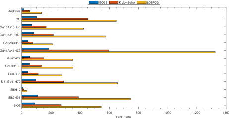
Figure 10. ${\tt tol}=10^{-4}$, ${\tt numEigen}=800$, and ${\tt numProc}=36$

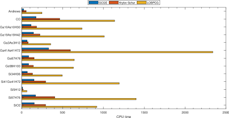
Figure 11. ${\tt tol}=10^{-8}$, ${\tt numEigen}=800$, and ${\tt numProc}=36$

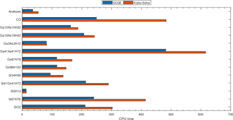
Figure 12. ${\tt tol}=10^{-12}$, ${\tt numEigen}=800$, and ${\tt numProc}=36$

Obviously, GCGE is always more efficient than LOBPCG under different tolerances. In addition, when ${\tt tol}=10^{-4}$ and $10^{-8}$, GCGE is much faster than Krylov-Schur method. Under tolerances $10^{-12}$, the CPU time of GCGE and Krylov-Shur method is similar and GCGE is slighly faster.

In addition, the convergence procedure of GCG algorithm with ${\tt tol}=10^{-12}$ for the first thirteen matrices is shown in Figure 13. As the number of GCG iterations increases, the number of converged eigenpairs increases. In Figure 14, the absolute residual of the first unconverged eigenpair is presented.

For FEM matrices, the performances of GCGE are shown in Figures 15 and 16. Due to ${\tt blockSize}={\tt numEigen}/5=40$, there are four noticeable pauses for the case of ${\tt tol}=10^{-12}$ when the number of converged eigenpairs is close to $1\times 40$, $2\times 40$, $3\times 40$, and $4\times 40$ at around the 40th, 60th, 80th, and 100th GCG iteration. Roughly speaking, the $40$ eigenpairs can be converged once every twenty GCG iterations.

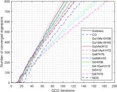
Figure 13. ${\tt tol}=10^{-12}$, ${\tt numEigen}=800$, and ${\tt numProc}=36$

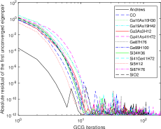
Figure 14. ${\tt tol}=10^{-12}$, ${\tt numEigen}=800$, and ${\tt numProc}=36$

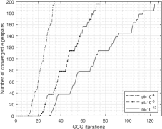
Figure 15. ${\tt numEigen}=200$ and ${\tt numProc}=576$

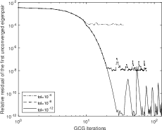
Figure 16. ${\tt numEigen}=200$ and ${\tt numProc}=576$

4.3. Scaling for the number of eigenpairs

Here, we investigate the dependence of computing time on the number of desired eigenpairs. For this aim, we compute the first $50$-$800$ eigenpairs of matrices listed in Table 2.

The test for the first thirteen matrices is performed on a single node with 36 processes. The results in Figures 17 and 18 show that just like LOBPCG, GCGE has almost linear scaling property, which means the computing time is linearly dependent on the number of desired eigenpairs. Moreover, GCGE has better efficiency than LOBPCG. From Andrews to SiO2, the total time ratios of GCGE to LOBPCG are

$$17.59\%,\ 19.17\%,\ 16.70\%,\ 15.02\%,\ 19.35\%,\ 15.46\%,$$

$$14.67\%,\ 14.43\%,\ 15.85\%,\ 14.44\%,\ 28.82\%,\ 14.15\%,\ 19.55\%.$$

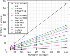
Figure 17. GCGE with ${\tt tol}=10^{-8}$ and ${\tt numProc}=36$

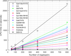
Figure 18. LOBPCG with ${\tt tol}=10^{-8}$ and ${\tt numProc}=36$

Since the scales of FEM matrices are large, the test is performed with $576$ processes on $16$ nodes. The dependence of CPU time (in seconds) for FEM matrices on the number of eigenpairs is shown in Figure 19, which implies that GCGE has better efficiency than LOBPCG for large scale matrices. Moreover, GCGE and LOBPCG both have almost linear scaling property for large scale FEM matrices.

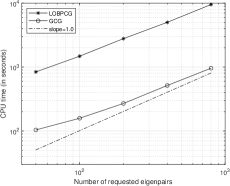
Figure 19. CPU time for FEM matrices with ${\tt tol}=10^{-8}$ and ${\tt numProc}=576$

Remark 4.1.

In fact, Krylov-Schur method is low efficient for FEM matrices on multi-nodes. In Table 5, for ${\tt numEigen}=50,100,200$, the generalized eigenvalue problem is tested, which is the discretization of the eigenvalue problem (18) for the conforming linear finite element (P1 element) with 3,145,728 elements. The dimensions of the matrices $A$ and $B$ are both 512,191.

Table 5. FEM matrices (P1 element) with ${\tt tol}=10^{-8}$ and ${\tt numProc}=36$

Method	50	100	200
GCGE	20.15	38.98	71.49
Krylov-Schur	1032.33	1360.56	2180.28
LOBPCG	63.99	114.65	286.67

4.4. Scalability test

In order to do the scalability test, we use $36$-$288$ processes to compute the first $800$ eigenpairs of the first thirteen matrices listed in Table 2. The comparisons of the scalability of GCGE and LOBPCG are shown in Figures 20, 21, 22 and Table 6. It is noted that GCGE, LOBPCG, and Krylov-Schur methods have similar scalability for the first thirteen matrices, but the total time ratios of GCGE to LOBPCG are

$$11.92\%,\ 10.10\%,\ 9.61\%,\ 8.79\%,\ 11.19\%,\ 8.37\%,$$

$$7.88\%,\ 8.10\%,\ 8.86\%,\ 7.93\%,\ 12.85\%,\ 7.82\%,\ 11.36\%,$$

from Andrews to SiO2. In other words, GCGE has better efficiency than LOBPCG. In addition, the total time ratios of GCGE to Krylov-Schur method are

$$107.63\%,\ 50.08\%,\ 80.26\%,\ 73.64\%,\ 114.66\%,\ 57.77\%,$$

$$69.20\%,\ 73.86\%,\ 75.06\%,\ 64.07\%,\ 143.52\%,\ 51.67\%,\ 70.54\%,$$

from Andrews to SiO2. Only for small scale matrices Andrews (60,000), Ga3As3H12 (61,349), and Si34H36 (97,567), the Krylov-Schur method is more efficient than GCGE, which are shown in Table 6.

Table 6. Small scale matrices with ${\tt tol}=10^{-8}$ and ${\tt numEigen}=800$

numProc	Method	Andrews	Ga3As3H12	Si5H12
36	GCGE	37.28	60.32	9.38
	Krylov-Schur	54.66	69.90	11.95
	LOBPCG	447.09	650.75	113.48
72	GCGE	26.09	39.85	7.65
	Krylov-Schur	26.34	34.13	5.30
	LOBPCG	247.59	353.91	62.59
144	GCGE	22.69	26.54	7.11
	Krylov-Schur	14.82	15.73	2.90
	LOBPCG	155.08	193.54	44.10
288	GCGE	34.55	20.36	8.64
	Krylov-Schur	16.22	8.49	2.69
	LOBPCG	162.46	115.88	34.98

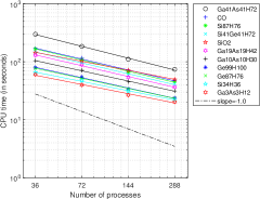
Figure 20. GCGE with ${\tt tol}=10^{-8}$ and ${\tt numEigen}=800$

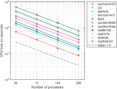
Figure 21. Krylov-Schur method with ${\tt tol}=10^{-8}$ and ${\tt numEigen}=800$

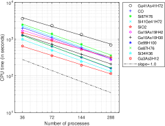
Figure 22. LOBPCG with ${\tt tol}=10^{-8}$ and ${\tt numEigen}=800$

About the large scale FEM matrices, we use $36$-$1152$ processes for computing the lowest $100$ and $200$ eigenpairs. In Figure 23, we can find that GCGE and LOBPCG have similar scalability for large scale matrices, but GCGE has better efficiency. And the total time ratio of GCGE to LOBPCG is about $10\%$.

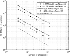
Figure 23. CPU time for FEM matrices with ${\tt tol}=10^{-8}$

4.5. The performance of GCGE with large numEigen

In this subsection, the performance of the moving mechanism presented in Section 3.3 is tested. The maximum project dimensions, ${\tt maxProjDim}$, are set to $1000$ and $2000$ for the first thirteen matrices and FEM matrices, respectively.

In Figure 24, the performance of GCGE with the moving mechanism is shown for the first thirteen matrices, For Krylov-Schur method, we set ${\tt numEigen}$ to be $2000$ and $4000$ and the parameters are

    -eps_nev 2000
    -eps_ncv 2400
    -eps_mpd 800

and

    -eps_nev 4000
    -eps_ncv 4400
    -eps_mpd 1000

respectively, such that Krylov-Schur method has best efficiency for comparison. Moreover, GCGE has better efficiency than Krylov-Schur. From Andrews to SiO2, the total time ratios of GCGE to Krylov-Schur are

$$32.04\%,\ 27.49\%,\ 41.38\%,\ 41.70\%,\ 54.18\%,\ 36.60\%,\ 33.72\%,$$

$$34.02\%,\ 31.76\%,\ 33.35\%,\ 50.08\%,\ 24.71\%,\ 35.05\%,\$$

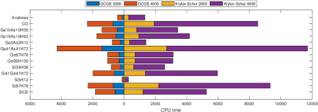
Figure 24. ${\tt tol}=10^{-12}$, ${\tt blockSize}=100$, and ${\tt numProc}=36$

For FEM matrices with ${\tt numEigen}=5000$, without the moving mechanism, the time of STEP 3 is dominated in Table 7. And with the moving mechanism, the total time is reduced by about $50\%$. In addition, the total time with dynamic shifts is reduced by about $20\%$ again due to the reduction of the total number of GCG iterations.

Table 7. The performance for FEM matrices with ${\tt tol}=10^{-8}$, ${\tt blockSize}=200$, and ${\tt numProc}=1152$.

	Without Moving Mechanism		With Moving Mechanism		With Dynamic Shifts
	Time	Percentage	Time	Percentage	Time	Percentage
STEP 2	445.05	5.33%	42.64	1.04%	41.56	1.25%
STEP 3	4727.57	56.65%	737.57	18.03%	601.92	18.17%
STEP 4	78.94	0.95%	34.09	0.83%	32.60	0.98%
STEP 5	281.12	3.37%	123.21	3.01%	99.52	3.00%
STEP 6	2811.89	33.70%	3153.00	77.08%	2537.38	76.59%
Total Time	8344.57	100.00%	4090.52	100.00%	3312.98	100.00%
Ratio	100.00%		49.02%		39.70%

In Table 8, the performances of two different orthogonalization methods are also compared. When numEigen = 10000, Algorithm 3 is faster than Algorithm 2 because of fewer multiplication of matrix and vectors, especially for the generalized algebraic eigenvalue problems.

Table 8. The performance for FEM matrices with ${\tt tol}=10^{-8}$, ${\tt blockSize}=200$, and ${\tt numProc}=1152$.

	Algorithm 2		Algorithm 3
	Time	Percentage	Time	Percentage
STEP 2	18.37	0.16%	18.35	0.17%
STEP 3	1992.81	17.58%	2025.87	18.45%
STEP 4	90.04	0.79%	66.93	0.61%
STEP 5	324.76	2.87%	326.45	2.97%
STEP 6	8907.10	78.59%	8544.80	77.80%
Total Time	11333.08	100.00%	10982.40	100.00%
Ratio	100.00%		96.90%

5. Concluding remarks

This paper highlights some new issues for computing plenty of eigenpairs of large scale matrices on high performance computers. The GCGE package is presented which is built with the damping block inverse power method with dynamic shifts for symmetric eigenvalue problems. Furthermore, in order to improve the efficiency, stability and scalability of the concerned package, the new efficient implementing techniques are designed for updating subspaces, orthogonalization and computing Rayleigh-Ritz problems. Plenty of numerical tests are provided to validate the proposed package GCGE, which can be downloaded from https://github.com/Materials-Of-Numerical-Algebra/GCGE.

- (1)
- Amestoy et al. (2019) P. R. Amestoy, A. Buttari, J. Y. L’Excellent, and T. Mary. 2019. Performance and scalability of the block low-rank multifrontal factorization on multicore architectures. ACM Trans. Math. Software 45, 1 (2019), 2:1–2:26.
- Amestoy et al. (2001) Patrick. R. Amestoy, Iain S. Duff, Jacko Koster, and Jean Yves L’Excellent. 2001. A fully asynchronous multifrontal solver using distributed dynamic scheduling. SIAM Journal on Matrix Analysis & Applications 23, 1 (2001), 15–41.
- Anderson et al. (1999) E. Anderson, Z. Bai, C. Bischof, S. Blackford, J. Demmel, J. Dongarra, J. Du Croz, A. GreenBaum, S. Hammarling, A. Mckenney, and D. Sorensen. 1999. LAPACK Users’ Guide. SIAM.
- Bai et al. (2000) Zhaojun Bai, James Demmel, Jack Dongarra, Axel Ruhe, and Henk van der Vorst. 2000. Templates for the Solution of Algebraic Eigenvalue Problems: A Practical Guide. Vol. 11. SIAM.
- Balay et al. (1997) Satish Balay, William D. Gropp, Lois Curfman McInnes, and Barry F. Smith. 1997. Efficient management of parallelism in object oriented numerical software libraries. In Modern Software Tools in Scientific Computing. Birkhäuser Press.
- Duersch et al. (2018) Meiyue Duersch, Jed A. amd Shao, Chao Yang, and Ming Gu. 2018. Robust and Efficient Implementation of LOBPCG. SIAM Journal on Scientific Computing 40, 5 (2018), 655–676.
- Falgout et al. (2006) Robert D Falgout, Jim E Jones, and Ulrike Meier Yang. 2006. The design and implementation of hypre, a library of parallel high performance preconditioners. In Numerical Solution of Partial Differential Equations on Parallel Computers. Springer, 267–294.
- Fan et al. (2014) Xuanhua Fan, Pu Chen, Rui-an Wu, and Shifu Xiao. 2014. Parallel computing of large-scale modal ananlysis based on Jacobi-Davidson algorithm. Journal of Vibration and Shock 33, 1 (2014), 203–208.
- Fan et al. (2015) Xuanhua Fan, Shifu Xiao, and Pu Chen. 2015. Parallel computing study on finite element modal analysis over ten-million degrees of freedom. Journal of Vibration and Shock 34, 17 (2015), 77–82.
- Hernandez et al. (2005) Vicente Hernandez, Jose E. Roman, and Vicente Vidal. 2005. SLEPc: A scalable and flexible toolkit for the solution of eigenvalue problems. ACM Trans. Math. Software 31, 3 (2005), 351–362.
- Hetmaniuk and Lehoucq (2006) U. Hetmaniuk and R. Lehoucq. 2006. Basis selection in LOBPCG. J. Comput. Phys. 218, 1 (2006), 324–332.
- Knyazev (2006) Andrew V. Knyazev. 2006. Toward the optimal preconditioned eigensolver: locally optimal block preconditioned conjugate gradient method. SIAM Journal on Scientific Computing 23, 2 (2006), 517–541.
- Knyazev et al. (2007) Andrew V Knyazev, Merico E Argentati, Ilya Lashuk, and Evgueni E Ovtchinnikov. 2007. Block locally optimal preconditioned eigenvalue xolvers (BLOPEX) in HYPRE and PETSc. SIAM Journal on Scientific Computing 29, 5 (2007), 2224–2239.
- Knyazev and Neymeyr (2003) Andrew V Knyazev and Klaus Neymeyr. 2003. Efficient solution of symmetric eigenvalue problems using multigrid preconditioners in the locally optimal block conjugate gradient method. Electronic Transactions on Numerical Analysis 15 (2003), 38–55.
- Kronik et al. (2006) Leeor Kronik, Adi Makmal, Murilo L. Tiago, M. M. G. Alemany, Manish Jain, Xiangyang Huang, Yousef Saad, and James R. Chelikowsky. 2006. PARSEC – the pseudopotential algorithm for real-space electronic structure calculations: recent advances and novel applications to nano-structures. Physica Status Solidi 243, 5 (2006), 1063–1079.
- Li et al. (2020) Yu Li, Hehu Xie, Ran Xu, Chun’Guang You, and Ning Zhang. 2020. A parallel generalized conjugate gradient method for large scale eigenvalue problems. CCF Transactions on High Performance Computing 2 (2020), 111–122.
- Natan et al. (2008) Amir Natan, Ayelet Benjamini, Doron Naveh, Leeor Kronik, Murilo L. Tiago, Scott P. Beckman, and James R. Chelikowsky. 2008. Real-space pseudopotential method for first principles calculations of general periodic and partially periodic systems. Physical Review B 78, 7 (2008), 75–109.
- Saad (1992) Youcef Saad. 1992. Numerical Methods for Large Eigenvalue Problems. Vol. 158. SIAM.
- Saad et al. (2010) Yousef Saad, James R. Chelikowsky, and Suzanne M. Shontz. 2010. Numerical methods for electronic structure calculations of materials. SIAM Rev. 52, 1 (2010), 3–54.
- Stewart (2008) G. W. Stewart. 2008. Block Gram–Schmidt Orthogonalization. SIAM Journal on Entific Computing 31, 1 (2008), 761–775.
- Yokozawa et al. (2006) Takuya Yokozawa, Daisuke Takahashi, Taisuke Boku, and Mitsuhisa Sato. 2006. Efficient parallel implementation of classical Gram-Schmidt orthogonalization using matrix multiplication. In Proceedings of Fourth International Workshop on Parallel matrix Algorithms and Applications (PMAA’06). 37–38.
- Yu et al. (2018) C. Yu, X. Fan, K. Wang, and S. Xiao. 2018. Parallel Computing of Multipoint-Base-Excited Harmonic Response with PANDA Platform. Jisuan Wuli/Chinese Journal of Computational Physics 35, 4 (2018), 443–450.
- Zhang (2009) Linbo Zhang. 2009. A parallel algorithm for adaptive local refinement of tetrahedral meshes using bisection. Numerical Mathematics: Theory, Methods and Applications 2 (2009), 65–89.
- Zhang et al. (2020) Ning Zhang, Yu Li, Hehu Xie, Ran Xu, and Chunguang You. 2020. A generalized conjugate gradient method for eigenvalue problems. SCIENTIA SINICA Mathematica 50, 12 (2020), 1–24.