A low-rank solution method for Riccati equations with indefinite quadratic terms

Abstract

Algebraic Riccati equations with indefinite quadratic terms play an important role in applications related to robust controller design. While there are many established approaches to solve these in case of small-scale dense coefficients, there is no approach available to compute solutions in the large-scale sparse setting. In this paper, we develop an iterative method to compute low-rank approximations of stabilizing solutions of large-scale sparse continuous-time algebraic Riccati equations with indefinite quadratic terms. We test the developed approach for dense examples in comparison to other established matrix equation solvers, and investigate the applicability and performance in large-scale sparse examples.

We propose an iterative algorithm for computing low-rank approximations of stabilizing solutions of continuous-time algebraic Riccati equations with indefinite quadratic term. This is the first such approach that applies for general setups with large-scale sparse coefficient matrices.

1 Introduction

Many concepts in systems and control theory are connected to solutions of algebraic Riccati equations. Prominent examples are the linear-quadratic regulator (LQR) and linear-quadratic Gaussian (LQG) controller design [57, 2, 46, 39] and corresponding model order reduction methods [36] as well as the characterization of passivity and contractivity of input-output systems and properties-preserving model reduction methods for these [28, 50, 3]. They also appear, for example, in applications with differential games [27, 6]. In this paper, we consider algebraic Riccati equations with indefinite quadratic terms of the form

$$A^{\mkern-1.5mu\mathsf{T}}XE+E^{\mkern-1.5mu\mathsf{T}}XA+E^{\mkern-1.5mu\mathsf{T}}X\left(B_{1}B_{1}^{\mkern-1.5mu\mathsf{T}}-B_{2}B_{2}^{\mkern-1.5mu\mathsf{T}}\right)XE+C^{\mkern-1.5mu\mathsf{T}}C =0,$$ (1)

with $A,E\in\mathbb{R}^{n\times n}$, $B_{1}\in\mathbb{R}^{n\times m_{1}}$, $B_{2}\in\mathbb{R}^{n\times m_{2}}$, $C\in\mathbb{R}^{p\times n}$ and $E$ invertible, and we are interested in symmetric positive semi-definite stabilizing solutions of Eq. 1. Equations of the form Eq. 1 usually occur in $\mathcal{H}_{\infty}$-control theory and related topics, e.g., robust controller design [47, 29, 49].

In the case of coefficients of small size $n$ and classical LQR/LQG Riccati equations, i.e., $B_{1}=0$ in Eq. 1 such that the quadratic term is negative semi-definite, there is a variety of different numerical approaches to compute the stabilizing solution: Direct approaches that compute eigenvalue decompositions of underlying Hamiltonian or even matrix pencils [42, 1, 4], iterative methods that work on the underlying spectrum of the Hamiltonian matrix [51, 7, 13], or iterative approaches, which compute a sequence of matrices converging to the stabilizing solution [37, 55]. The problem becomes more complicated in the opposite case with symmetric positive semi-definite quadratic term, i.e., in Eq. 1 setting $B_{2}=0$, which occurs in bounded-real and positive-real problems [28, 50, 3]. This already reduces the number of applicable methods. While methods from the classical setting that do not take the definiteness of the quadratic term into account can still be applied here [42, 4, 51, 7], only few, iterative Newton-type methods, which converge to the desired solution, have been developed for this problem class [22, 61, 8]. The amount of applicable methods narrows down even further when considering the general case of indefinite quadratic terms like in Eq. 1. A new type of iterative method for the solution of Eq. 1 was developed in [40, 41] to overcome accuracy problems of classical solution approaches and the general lack of iterative methods for this problem type. This new method computes a sequence of matrices converging to the stabilizing solution of Eq. 1 by solving classical Riccati equations with symmetric negative semi-definite quadratic terms.

However, in this paper, we will mainly focus on the case of large-scale sparse coefficient matrices in Eq. 1 arising, for example, from the discretization of partial differential equations, with $n\gtrapprox 10^{5}$ and low-rank quadratic term and right-hand side such that $m_{1},m_{2},p\ll n$. This leads to another multitude of problems. First of all, the dense computation methods from above cannot be applied anymore since they may transform the original data and compute full solutions, which easily becomes unfeasible in terms of memory requirements. Also, these methods usually use matrix operations that cannot be efficiently used in the large-scale sparse setting, which heavily increases the running time of algorithms. As in the dense case, there exists a variety of methods for the classical LQR/LQG case ($B_{1}=0$), for example, the low-rank Newton method [20, 62] with an underlying low-rank alternating direction implicit method [44, 20, 18, 19, 38] for solving the occurring large-scale sparse Lyapunov equations (LR-Newton-ADI), the Riccati alternating direction implicit method (RADI) [11], the incremental low-rank subspace iteration (ILRSI) [45], and projection-based methods that construct approximating subspaces such that internally small-scale dense Riccati equations need to be solved, e.g., [35, 56]. See also [21, 12, 38] for overviews and numerical comparisons of large-scale sparse solvers for this special case of Riccati equations with negative semi-definite quadratic terms. For the opposite case of Riccati equations with positive semi-definite quadratic terms ($B_{2}=0$), only the Newton method from [22] is known to have a low-rank extension to the large-scale sparse matrix case. However, there are no methods known to solve the general case Eq. 1 with an indefinite quadratic term in the large-scale sparse setting. The goal of this paper is to develop an extension of the approach described in [40, 41] that can be applied in the case of large-scale sparse coefficient matrices.

In the upcoming Section 2, we first recap the algorithm from [40, 41] and summarize some important results. Afterwards, we reformulate the steps of the algorithm to fit the large-scale sparse system case and extend it further to singular $E$ matrices arising in certain applications. In Section 3, we test the new algorithm first on Riccati equations with dense coefficients, for a comparison to other established methods, and afterwards on equations with large-scale sparse coefficients. The paper is concluded in Section 4.

2 Riccati iteration method

In this section, we describe the idea of the Riccati iteration method from [40, 41] and extend the approach to large-scale sparse systems.

Thereby, we will use the following notation. We will denote symmetric positive semi-definite matrices by $X=X^{\mkern-1.5mu\mathsf{T}}\geq 0$, for $X\in\mathbb{R}^{n\times n}$, and use the Loewner ordering $X_{1}\geq X_{2}$ for two symmetric matrices $X_{1},X_{2}\in\mathbb{R}^{n\times n}$, if $X_{1}-X_{2}\geq 0$. We call the matrix triple $(A,B,E)$ stabilizable, with $A,E\in\mathbb{R}^{n\times n}$, $B\in\mathbb{R}^{n\times m}$ and $E$ invertible, if there exists a feedback matrix $K\in\mathbb{R}^{m\times n}$ such that the matrix pencil $\lambda E-(A-BK)$ has only eigenvalues with negative real parts.

2.1 Basic algorithm

In this section, we formulate the fundamental algorithms for the iterative computation of approximate solutions to the following general problem.

Problem 1 (Stabilizing solutions of indefinite Riccati equations).

Given matrices $A,E\in\mathbb{R}^{n\times n}$, $B_{1}\in\mathbb{R}^{n\times m_{1}}$, $B_{2}\in\mathbb{R}^{n\times m_{2}}$ and $C\in\mathbb{R}^{p\times n}$, with $E$ invertible and $n$, $m_{1}$, $m_{2}$, $p\in\mathbb{N}$, compute a matrix $X=X_{\infty}\in\mathbb{R}^{n\times n}$, if it exists,

• which solves the Riccati equation (1) with indefinite quadratic term

  $$A^{\mkern-1.5mu\mathsf{T}}XE+E^{\mkern-1.5mu\mathsf{T}}XA+E^{\mkern-1.5mu\mathsf{T}}X\left(B_{1}B_{1}^{\mkern-1.5mu\mathsf{T}}-B_{2}B_{2}^{\mkern-1.5mu\mathsf{T}}\right)XE+C^{\mkern-1.5mu\mathsf{T}}C =0,\quad\text{and}$$

• which is symmetric positive semi-definite and such that the pencil

  $$\lambda E-\big{(}A+(B_{1}B_{1}^{\mkern-1.5mu\mathsf{T}}-B_{2}B_{2}^{\mkern-1.5mu\mathsf{T}})X_{\infty}E\big{)}$$

  is stable, i.e., all its eigenvalues lie in the open left half-plane.

For computing the solution to Problem 1 numerically, the Riccati iteration method was first described in [40, 41] for the standard equation case ($E=I_{n}$). Here, we will summarize the method and some theoretical results using directly the generalized case with $E$ invertible. The underlying idea of the algorithm is to consider the Riccati operator

$$\mathcal{R}(X) :=A^{\mkern-1.5mu\mathsf{T}}XE+E^{\mkern-1.5mu\mathsf{T}}XA-E^{\mkern-1.5mu\mathsf{T}}X(B_{2}B_{2}^{\mkern-1.5mu\mathsf{T}}-B_{1}B_{1}^{\mkern-1.5mu\mathsf{T}})XE+C_{1}^{\mkern-1.5mu\mathsf{T}}C_{1},$$ (2)

associated with Eq. 1, and a splitting of the final solution into the sum of consecutive solutions of updated algebraic Riccati equations with semi-definite quadratic terms. For two symmetric matrices $X_{1}=X_{1}^{\mkern-1.5mu\mathsf{T}}$ and $X_{2}=X_{2}^{\mkern-1.5mu\mathsf{T}}$, one can show that

$$\mathcal{R}(X_{1}+X_{2}) =\mathcal{R}(X_{1})+{\widetilde{A\mkern 4.0mu}\mkern-4.0mu}{}^{\mkern-1.5mu\mathsf{T}}X_{2}E+E^{\mkern-1.5mu\mathsf{T}}X_{2}{\widetilde{A\mkern 4.0mu}\mkern-4.0mu}{}-E^{\mkern-1.5mu\mathsf{T}}X_{2}(B_{2}B_{2}^{\mkern-1.5mu\mathsf{T}}-B_{1}B_{1}^{\mkern-1.5mu\mathsf{T}})X_{2}E$$

holds, where ${\widetilde{A\mkern 4.0mu}\mkern-4.0mu}{}:=A-(B_{2}B_{2}^{\mkern-1.5mu\mathsf{T}}-B_{1}B_{1}^{\mkern-1.5mu\mathsf{T}})X_{1}E$. Accordingly, for $X_{2}$ as a solution to the algebraic Riccati equation with negative semi-definite quadratic term

$$0 =\mathcal{R}(X_{1})+{\widetilde{A\mkern 4.0mu}\mkern-4.0mu}{}^{\mkern-1.5mu\mathsf{T}}X_{2}E+E^{\mkern-1.5mu\mathsf{T}}X_{2}{\widetilde{A\mkern 4.0mu}\mkern-4.0mu}{}-E^{\mkern-1.5mu\mathsf{T}}X_{2}B_{2}B_{2}^{\mkern-1.5mu\mathsf{T}}X_{2}E,$$ (3)

the residual reads

$$\mathcal{R}(X_{1}+X_{2}) =E^{\mkern-1.5mu\mathsf{T}}X_{2}B_{1}B_{1}^{\mkern-1.5mu\mathsf{T}}X_{2}E.$$

An iterative use of this relation Eq. 3, together with the initial solution $X_{0}=0$, yields the Riccati iteration (RI) method. The resulting algorithm is given in Algorithm 1.

1

2

Input: $A,B_{1},B_{2},C,E$ from Eq. 1, convergence tolerance $\tau$.

Output: Stabilizing approximate solution $X_{k}\approx X_{\infty}$ of Eq. 1, with $X_{k}=X_{k}^{\mkern-1.5mu\mathsf{T}}\geq 0$.

3

4Initialize $X_{0}=0$, $k=0$.

5

6repeat

7       Update the iteration matrix $A_{k}=A+(B_{1}B_{1}^{\mkern-1.5mu\mathsf{T}}-B_{2}B_{2}^{\mkern-1.5mu\mathsf{T}})X_{k}E$.

8      

9      Solve the definite Riccati equation

$$A_{k}^{\mkern-1.5mu\mathsf{T}}W_{k+1}E+E^{\mkern-1.5mu\mathsf{T}}W_{k+1}A_{k}-E^{\mkern-1.5mu\mathsf{T}}W_{k+1}B_{2}B_{2}^{\mkern-1.5mu\mathsf{T}}W_{k+1}E+\mathcal{R}(X_{k}) =0$$

for the stabilizing solution $W_{k+1}\in\mathbb{R}^{n\times n}$.

10      

11      Update the solution matrix $X_{k+1}=X_{k}+W_{k+1}$. 

12      if $(A+B_{1}B_{1}^{\mkern-1.5mu\mathsf{T}}X_{k+1}E,B_{2},E)$ is stabilizable then

13             Increment $k\leftarrow k+1$.

14            

15      else

             error // There is no stabilizing $X=X^{\mkern-1.5mu\mathsf{T}}\geq 0$ that solves Eq. 1.

16            

17       end if

18      

19until $\lVert B_{1}W_{k}E\rVert_{2}<\tau$

Algorithm 1 Riccati iteration (RI).

The following proposition lays out the theoretical foundation of the Riccati iteration method.

Proposition 1 (Properties of the Riccati iteration [40, 41]).

If $(A,B_{2},E)$ is stabilizable, $(A,C,E)$ has no unobservable purely imaginary modes and there exists a stabilizing solution $X_{\infty}=X_{\infty}^{\mkern-1.5mu\mathsf{T}}\geq 0$ for Eq. 1, then the following statements hold for the iteration in Algorithm 1:

1. $(A+B_{1}B_{1}^{\mkern-1.5mu\mathsf{T}}X_{k}E,B_{2},E)$ is stabilizable for all $k=0,1,\ldots$,

2. $W_{k}=W_{k}^{\mkern-1.5mu\mathsf{T}}\geq 0$ for all $k=0,1,\ldots$,

3. the eigenvalues of the matrix pencil $\lambda E-(A+B_{1}B_{1}^{\mkern-1.5mu\mathsf{T}}X_{k}E-B_{2}B_{2}X_{k+1}E)$ lie in the left open half-plane for all $k=0,1,\ldots$,

4. $\mathcal{R}(X_{k+1})=E^{\mkern-1.5mu\mathsf{T}}W_{k+1}B_{1}B_{1}^{\mkern-1.5mu\mathsf{T}}W_{k+1}E$ for all $k=0,1,\ldots$,

5. $X_{\infty}\geq\ldots\geq X_{k+1}\geq\ldots\geq X_{1}\geq X_{0}=0$,

6. the iteration converges to the stabilizing solution of Eq. 1, $\lim_{k\rightarrow\infty}X_{k}=X_{\infty}$, and

7. the convergence is locally quadratic.

Basically, the conditions of Proposition 1 guarantee convergence of the iterants to the desired solution of Problem 1 as well as the stabilization property for every intermediate iteration step. The following remark gives some insight about the convergence of the stabilizing solutions of Eq. 1 and the convergence of the Riccati iteration.

Remark 1 (Definiteness of stabilizing solutions).

In general, if a real stabilizing solution of Eq. 1 exists, it does not need to be symmetric positive semi-definite; see examples in [40]. Other approaches that rely on the underlying Hamiltonian matrix pencil of Eq. 1 are capable of computing also indefinite stabilizing solutions. However, these are undesired in many applications. The Riccati iteration converges only if the stabilizing solution exists and it is symmetric positive semi-definite, which follows from Parts (e) and (f) of Proposition 1 and classical theory about the LQR/LQG Riccati equations that are solved in every iteration step.

2.2 Factorized low-rank formulation for large-scale sparse equations

The Riccati iteration method in Algorithm 1 cannot be directly applied to the large-scale case. Most importantly, the iterants $X_{k}$ will be dense $n\times n$-matrices such that memory will become a limiting factor already for moderate dimensions $n$. With the guarantee that all intermediate solutions $X_{k}$ as well as all updates $W_{k+1}$ are symmetric positive semi-definite (cf. Parts (a) and (e) of Proposition 1), the approximation by low-rank factorizations provides a potential remedy as in the symmetric semi-definite case; see, e.g., [21, 12]. The basic idea is to rewrite the intermediate stages of the Riccati iteration via Cholesky-like low-rank factorizations such that $X_{k}\approx Z_{k}Z_{k}^{\mkern-1.5mu\mathsf{T}}$ and $W_{k+1}\approx Y_{k+1}Y_{k+1}^{\mkern-1.5mu\mathsf{T}}$, with $Z_{k}\in\mathbb{R}^{n\times r_{k}}$ and $Y_{k+1}\in\mathbb{R}^{n\times q_{k+1}}$ for all $k=0,1,\ldots$ and the relevant equations in terms of the factors $Z_{k}$ and $Y_{k}$. In particular, with the intermediate solution in Step 6 of Algorithm 1 reformulated as

$$Z_{k+1}Z_{k+1}^{\mkern-1.5mu\mathsf{T}}\approx X_{k+1}=X_{k}+W_{k+1}\approx Z_{k}Z_{k}^{\mkern-1.5mu\mathsf{T}}+Y_{k+1}Y_{k+1}^{\mkern-1.5mu\mathsf{T}}=\begin{bmatrix}Z_{k}&Y_{k+1}\end{bmatrix}\begin{bmatrix}Z_{k}^{\mkern-1.5mu\mathsf{T}}\\ Y_{k+1}^{\mkern-1.5mu\mathsf{T}}\end{bmatrix},$$

we will develop an iteration for the solution factors without ever forming the full solution explicitly.

The residual Riccati equation in Step 4 of Algorithm 1 that defines the update $W_{k+1}$ is given via

$$A_{k}^{\mkern-1.5mu\mathsf{T}}W_{k+1}E+E^{\mkern-1.5mu\mathsf{T}}W_{k+1}A_{k}-E^{\mkern-1.5mu\mathsf{T}}W_{k+1}B_{2}B_{2}^{\mkern-1.5mu\mathsf{T}}W_{k+1}E+\mathcal{R}(X_{k}) =0,$$ (4)

and we observe that

1. in the initial step with $X_{0}=0$, we have $\mathcal{R}(X_{0})=C^{\mkern-1.5mu\mathsf{T}}C$, and

2. for all all further steps, with Part (d) of Proposition 1, it holds

   $$\mathcal{R}(X_{k+1}) =E^{\mkern-1.5mu\mathsf{T}}W_{k+1}B_{1}B_{1}^{\mkern-1.5mu\mathsf{T}}W_{k+1}E=\underbrace{\big{(}B_{1}^{\mkern-1.5mu\mathsf{T}}W_{k+1}E\big{)}^{\mkern-1.5mu\mathsf{T}}}_{\phantom{\,\mathbb{R}^{n\times m_{1}}}\in\,\mathbb{R}^{n\times m_{1}}}\underbrace{\big{(}B_{1}^{\mkern-1.5mu\mathsf{T}}W_{k+1}E\big{)}}_{\phantom{\,\mathbb{R}^{m_{1}\times n}}\in\,\mathbb{R}^{m_{1}\times n}},$$

   for all $k=0,1,\ldots$, and where $W_{k+1}\approx Y_{k+1}Y_{k+1}^{\mkern-1.5mu\mathsf{T}}$.

In both cases, this central step of the algorithm requires the solve of a standard (semi-definite) Riccati equation with low-rank factorized quadratic and constant terms. Accordingly, a low-rank factorized approximation to $X_{k+1}$ can be computed by established Riccati equation solvers, like the LR-Newton-ADI method [20, 62], RADI [11], ILRSI [45], or projection-based methods [35, 56].

Remark 2 (Low-rank solutions).

By the low-rank structure of the right hand-side and the quadratic terms, $m_{1},m_{2},p\ll n$, we can also expect the solution and update terms to be well approximated by low-rank factors such that $r_{k},q_{k}\ll n$; see [10, 58].

Combining all these ideas leads now to the low-rank Riccati iteration (LR-RI) method in Algorithm 2. Algorithm 2 has been implemented for dense coefficients in the MORLAB toolbox [25, 26] and for the large-scale sparse case in the M-M.E.S.S. toolbox [53, 17].

1

Input: $A,B_{1},B_{2},C,E$ from Eq. 1, convergence tolerance $\tau$.

Output: Low-rank factor $Z_{k}$ s.t. $Z_{k}Z_{k}^{\mkern-1.5mu\mathsf{T}}\approx X_{\infty}$ is the stabilizing solution of Eq. 1.

2

3Solve the Riccati equation with negative semi-definite quadratic term

$$A^{\mkern-1.5mu\mathsf{T}}W_{0}E+E^{\mkern-1.5mu\mathsf{T}}W_{0}A-E^{\mkern-1.5mu\mathsf{T}}W_{0}B_{2}B_{2}^{\mkern-1.5mu\mathsf{T}}W_{0}E+C^{\mkern-1.5mu\mathsf{T}}C =0,$$

for the low-rank factor $Y_{0}$ such that $Y_{0}Y_{0}^{\mkern-1.5mu\mathsf{T}}\approx W_{0}$.

4

5Initialize $Z_{0}=Y_{0}$, $U=\begin{bmatrix}B_{1}&-B_{2}\end{bmatrix}$ and $k=0$.

6

7while $\lVert B_{1}^{\mkern-1.5mu\mathsf{T}}Y_{k}Y_{k}^{\mkern-1.5mu\mathsf{T}}E\rVert_{2}>\tau$ do

8       Set $A_{k}=A-UV_{k}^{\mkern-1.5mu\mathsf{T}}$ with the updated low-rank factor

$$V_{k} =\begin{bmatrix}E^{\mkern-1.5mu\mathsf{T}}Z_{k}Z_{k}^{\mkern-1.5mu\mathsf{T}}B_{1}&E^{\mkern-1.5mu\mathsf{T}}Z_{k}Z_{k}^{\mkern-1.5mu\mathsf{T}}B_{2}\end{bmatrix}.$$

9      

10      Solve the Riccati equation with negative semi-definite quadratic term

$$A_{k}^{\mkern-1.5mu\mathsf{T}}W_{k+1}E+E^{\mkern-1.5mu\mathsf{T}}W_{k+1}A_{k}-E^{\mkern-1.5mu\mathsf{T}}W_{k+1}B_{2}B_{2}^{\mkern-1.5mu\mathsf{T}}W_{k+1}E+\big{(}E^{\mkern-1.5mu\mathsf{T}}W_{k}B_{1}\big{)}\big{(}E^{\mkern-1.5mu\mathsf{T}}W_{k}B_{1}\big{)}^{\mkern-1.5mu\mathsf{T}} =0,$$

for the low-rank factor $Y_{k+1}$ with $Y_{k+1}Y_{k+1}^{\mkern-1.5mu\mathsf{T}}\approx W_{k+1}$.

11      

12      Update $Z_{k+1}=\begin{bmatrix}Z_{k}&Y_{k+1}\end{bmatrix}$ and increment $k\leftarrow k+1$.

13      

14 end while

Algorithm 2 Low-rank Riccati iteration (LR-RI).

Another difference of Algorithm 2 compared to Algorithm 1 is the stabilizability test for $(A+B_{1}B_{1}^{\mkern-1.5mu\mathsf{T}}X_{k+1}E,B_{2},E)$. This additional test is expensive in the large-scale setting but can, in principle, be omitted. In case of $(A+B_{1}B_{1}^{\mkern-1.5mu\mathsf{T}}X_{k+1}E,B_{2},E)$ not being stabilizable in intermediate steps, the iteration will diverge and there might be no stabilizing solutions for the intermediate Riccati equations with negative semi-definite quadratic terms anymore. The following remarks state further computational features of the new low-rank iteration method in Algorithm 2.

Remark 3 (Unstable closed-loop matrix pencils).

The intermediate closed-loop matrix pencils $sE-A_{k}$ can potentially have unstable eigenvalues [41]. However, in case there exists a stabilizing solution $X_{\infty}=X_{\infty}^{\mkern-1.5mu\mathsf{T}}\geq 0$ of Eq. 1, $(A_{k},B_{2},E)$ will be stabilizable. Many of the low-rank solvers for definite Riccati equations need a stabilizing initial solution or a corresponding feedback matrix. In the large-scale sparse case, this can be computed using a sparse eigenvalue solver to compute the eigenvectors corresponding to the unstable eigenvalues of $sE-A_{k}$ and to apply a partial stabilization approach [9] on the projected problem using the computed eigenvalue basis [5]. Note that if $sE-A_{k_{0}}$ is stable for some $k_{0}$ and the iteration converges, then $sE-A_{k}$ will also be stable for all $k\geq k_{0}$; cf. Proposition 1.

Remark 4 (Solution of Riccati equations with positive semi-definite quadratic terms).

The Riccati iteration method can be used as an alternative approach to solve Riccati equations with positive semi-definite quadratic terms by setting $B_{2}=0$:

$$A^{\mkern-1.5mu\mathsf{T}}XE+E^{\mkern-1.5mu\mathsf{T}}XA+E^{\mkern-1.5mu\mathsf{T}}XB_{1}B_{1}^{\mkern-1.5mu\mathsf{T}}XE+C^{\mkern-1.5mu\mathsf{T}}C =0,$$

which occur, for example, in [28, 50, 3]. A necessary condition for applying the Riccati iteration method is in this case the stability of the matrix pencil $sE-A$, since otherwise the stabilizability of $(A,B_{2},E)$ will never be fulfilled. This problem does not occur in the Newton iteration from [22, 61, 8], where only a stabilizing initial feedback is needed.

2.3 Realization of linear solves in factored form

In general, the coefficients $A_{k}=A+(B_{1}B_{1}^{\mkern-1.5mu\mathsf{T}}-B_{2}B_{2}^{\mkern-1.5mu\mathsf{T}})X_{k}E$, for $k=1,2,\ldots$, of the intermediate Riccati equations in Step 4 of Algorithm 2 are $n\times n$-matrices without sparsity structures such that an explicit realization would make the approach infeasible in the large-scale setting. In this case, the coefficients need to be rewritten as the sparse system matrix $A$ plus low-rank update:

$$A_{k} =A+(B_{1}B_{1}^{\mkern-1.5mu\mathsf{T}}-B_{2}B_{2}^{\mkern-1.5mu\mathsf{T}})X_{k}E=A+\begin{bmatrix}B_{1}&-B_{2}\end{bmatrix}\begin{bmatrix}B_{1}^{\mkern-1.5mu\mathsf{T}}X_{k}E\\ B_{2}^{\mkern-1.5mu\mathsf{T}}X_{k}E\end{bmatrix}=:A+UV_{k}^{\mkern-1.5mu\mathsf{T}},$$ (5)

with $U,V_{k}\in\mathbb{R}^{n\times(m_{1}+m_{2})}$, for all $k=1,2,\ldots$. Thereby, matrix-vector multiplications with $A_{k}$ can be performed without resorting to an explicit formation of $A_{k}$.

For the use within sparse direct solvers, this factored representation of $A_{k}$ can be exploited as follows. Consider the shifted linear system

$$(\sigma E^{\mkern-1.5mu\mathsf{T}}-A_{k}^{\mkern-1.5mu\mathsf{T}})X =(\sigma E^{\mkern-1.5mu\mathsf{T}}-A^{\mkern-1.5mu\mathsf{T}}-V_{k}U^{\mkern-1.5mu\mathsf{T}})X=F,$$ (6)

for a slim right-hand side $F\in\mathbb{R}^{n\times\ell}$, with $\ell\ll n$, and a shift $\sigma\in\mathbb{C}$. The solution of such linear systems Eq. 6 are the backbone of standard iterative solvers for large-scale Riccati equations. By the Sherman-Morrison-Woodbury formula for matrix inversion [31] and with the abbreviation $\Phi(\sigma):=(\sigma E^{\mkern-1.5mu\mathsf{T}}-A^{\mkern-1.5mu\mathsf{T}})$, the inverse of the shifted matrix in Eq. 6 is given by

$$\big{(}\Phi(\sigma)-V_{k}U^{\mkern-1.5mu\mathsf{T}}\big{)}^{-1} =\Phi(\sigma)^{-1}+\Phi(\sigma)^{-1}V_{k}\big{(}I_{m_{1}+m_{2}}-U^{\mkern-1.5mu\mathsf{T}}\Phi(\sigma)^{-1}V_{k}\big{)}^{-1}U^{\mkern-1.5mu\mathsf{T}}\Phi(\sigma)^{-1},$$ (7)

which actually amounts to $2\ell$ sparse linear solves with $\sigma E^{\mkern-1.5mu\mathsf{T}}-A^{\mkern-1.5mu\mathsf{T}}$ and one solve with an $(m_{1}+m_{2})\times(m_{1}+m_{2})$-dimensional matrix. Thus, in a practical realization of Eq. 7 for Eq. 6, one would compute

$$X =Z_{1}+Z_{2}\big{(}I_{m_{1}+m_{2}}-U^{\mkern-1.5mu\mathsf{T}}Z_{2}\big{)}^{-1}U^{\mkern-1.5mu\mathsf{T}}Z_{1},$$

with $(\sigma E^{\mkern-1.5mu\mathsf{T}}-A^{\mkern-1.5mu\mathsf{T}})Z_{1}=F$, and $(\sigma E^{\mkern-1.5mu\mathsf{T}}-A^{\mkern-1.5mu\mathsf{T}})Z_{2}=V_{k}$.

An alternative to the Sherman-Morrison-Woodbury formula is the augmented matrix approach, which makes use of the block matrix inversion formula. This approach is, often times, more stable than the Sherman-Morrison-Woodbury formula. Thereby, the solution of Eq. 6 is given as the solution of an augmented system of linear equations with

$$\begin{bmatrix}\sigma E^{\mkern-1.5mu\mathsf{T}}-A^{\mkern-1.5mu\mathsf{T}}&V_{k}\\ U^{\mkern-1.5mu\mathsf{T}}&I_{m_{1}+m_{2}}\end{bmatrix}\begin{bmatrix}X\\ X^{\perp}\end{bmatrix} =\begin{bmatrix}F\\ 0\end{bmatrix},$$ (8)

where the lower block of the solution, $X^{\perp}$, is an auxiliary variable with no relevance for the solution. Under the assumption that $U$ and $V_{k}$ have much fewer columns than $n$, systems of the form Eq. 8 can still be solved with standard sparse solvers.

2.4 Singular $\boldsymbol{E}$ matrices and projected Riccati equations

A regular occurring case in applications involves singular $E$ matrices. These especially occur in control problems with differential-algebraic equations (DAEs). In general, the presence of singular $E$ matrices changes the concepts of stabilizability of matrix pencils and solvability of Riccati equations; see, e.g., [48, 32, 15] and references therein. However, in many cases, the singular part of $E$ does not play any substantial role and it is actually enough to consider the solution of Riccati equations restricted to subspaces corresponding to the finite eigenvalues of the matrix pencil $\lambda E-A$, i.e., a restriction to the invertible part of $E$. This can be realized in two different concepts:

1. consider a projected version of the Riccati equation Eq. 1 with additional constraints on the stabilizing solution,

2. consider a truncated version of the Riccati equation Eq. 1.

In the following subsections, we consider first the general ideas for projected and truncated Riccati equations and, afterwards, the setup of incompressible flows as a particular example.

2.4.1 Projected and truncated equations

In the first concept, appropriate spectral projections $\mathcal{P}_{r},\mathcal{P}_{\ell}\in\mathbb{R}^{n\times n}$ onto the right and left deflating subspaces corresponding to the finite eigenvalues of $\lambda E-A$ are explicitly introduced in Eq. 1 such that

$$A^{\mkern-1.5mu\mathsf{T}}XE+E^{\mkern-1.5mu\mathsf{T}}XA+E^{\mkern-1.5mu\mathsf{T}}X\left(B_{1}B_{1}^{\mkern-1.5mu\mathsf{T}}-B_{2}B_{2}^{\mkern-1.5mu\mathsf{T}}\right)XE+\mathcal{P}_{r}^{\mkern-1.5mu\mathsf{T}}C^{\mkern-1.5mu\mathsf{T}}C\mathcal{P}_{r} =0,$$ (9a)

$$\mathcal{P}_{\ell}^{\mkern-1.5mu\mathsf{T}}X\mathcal{P}_{\ell} =X,$$ (9b)

needs to be solved instead. While in general, such projections $\mathcal{P}_{r},\mathcal{P}_{\ell}$ can be constructed using decompositions of the matrix pencil $\lambda E-A$ that resemble the Weierstrass canonical form, they are in fact known for several specially structured problems that arise in the large-scale sparse setting; see [59] and the examples in [60, 23]. Note that the $E$ matrix in Eq. 9 is still singular, but the equation and its solutions are restricted to the appropriate underlying subspace. Iterative methods like Algorithm 2 can be used to solve Eq. 9, where only the application of the spectral projections $\mathcal{P}_{r}$ and $\mathcal{P}_{\ell}$ is needed in the intermediate computational steps. This is also the common drawback of solving Eq. 9, since the repeated application of the projections can quickly become expensive, especially in the large-scale sparse case.

The second concept of truncated Riccati equations is more commonly used in practice. Thereby, we consider in general Riccati equations of the form

$$\widehat{A}^{\mkern-1.5mu\mathsf{T}}\widehat{X}\widehat{E}+\widehat{E}^{\mkern-1.5mu\mathsf{T}}\widehat{X}\widehat{A}+\widehat{E}^{\mkern-1.5mu\mathsf{T}}\widehat{X}\left(\widehat{B}_{1}\widehat{B}_{1}^{\mkern-1.5mu\mathsf{T}}-\widehat{B}_{2}\widehat{B}_{2}^{\mkern-1.5mu\mathsf{T}}\right)\widehat{X}\widehat{E}+\widehat{C}^{\mkern-1.5mu\mathsf{T}}\widehat{C} =0,$$ (10)

where the truncated matrices are constructed by

$$\begin{aligned} \widehat{A}&=W^{\mkern-1.5mu\mathsf{T}}AV,&\widehat{E}&=W^{\mkern-1.5mu\mathsf{T}}EV,&\widehat{B}&=W^{\mkern-1.5mu\mathsf{T}}B,&\widehat{C}&=CV,\end{aligned}$$ (11)

with the coefficient matrices from Eq. 1 and $V,W\in\mathbb{R}^{n\times r}$, basis matrices of the right and left deflating subspaces corresponding to the finite eigenvalues of $\lambda E-A$. By construction, the $E$ matrix in Eq. 10 is nonsingular and the solution techniques mentioned so far for Eq. 1 can also be applied to Eq. 10. These basis matrices $V$ and $W$ can be computed and applied explicitly to Eq. 1 up to medium-scale sized coefficient matrices. This is backbone of the implementation of model reduction methods for descriptor systems in the MORLAB toolbox [25, 26] and explained, e.g., in [24].

However, the explicit computation of the basis matrices $V$ and $W$ and of the resulting truncated coefficient matrices Eq. 11 is usually not possible in the large-scale sparse setting because of computation time and memory limitations. In this case, for many special sparse structures, the truncated Riccati equation Eq. 10 can be realized implicitly during the computations, i.e., instead of applying Algorithm 2 directly to Eq. 10, the original sparse coefficients from Eq. 1 are used and, by means of their structure, $V$ and $W$ are implicitly applied during the computational steps. Examples for this implicit truncation are given for different sparsity structures in [54, 5, 34, 30], which are also implemented in the function handle framework of the M-M.E.S.S. toolbox [53, 17]. Consequently, the implementation of Algorithm 2 in the M-M.E.S.S. toolbox can make use of the implicit truncation in case of singular $E$ matrices. As a particular example, the following subsection considers the case of structured coefficient matrices arising from incompressible flows.

2.4.2 Implicit realization of truncations in case of flow problems

Riccati equations with indefinite quadratic terms Eq. 1 are of particular interest in the design of robust controllers for the stabilization of incompressible flows modeled by linearization of the Navier-Stokes equations [16]. We briefly touch this particular case as an example for implicit truncation since we will consider such a numerical example later. In this case, the coefficient matrices of Eq. 1 are structured and given by

$$\begin{aligned} A&=\begin{bmatrix}{\widetilde{A\mkern 4.0mu}\mkern-4.0mu}{}&J^{\mkern-1.5mu\mathsf{T}}\\ J&0\end{bmatrix},&E&=\begin{bmatrix}{\widetilde{E\mkern 4.0mu}\mkern-4.0mu}{}&0\\ 0&0\end{bmatrix},&B_{1}&=\begin{bmatrix}{\widetilde{B\mkern 4.0mu}\mkern-4.0mu}{}_{1}\\ 0\end{bmatrix},&B_{2}&=\begin{bmatrix}{\widetilde{B\mkern 4.0mu}\mkern-4.0mu}{}_{2}\\ 0\end{bmatrix},&C&=\begin{bmatrix}{\widetilde{C\mkern 4.0mu}\mkern-4.0mu}{}&0\end{bmatrix},\end{aligned}$$ (12)

with ${\widetilde{E\mkern 4.0mu}\mkern-4.0mu}{}$ symmetric and invertible. The key to implicitly truncate and project Riccati equations with coefficients like Eq. 12 is the discrete Leray projection

$$\Pi =I_{\tilde{n}}-{\widetilde{E\mkern 4.0mu}\mkern-4.0mu}{}^{-1}J^{\mkern-1.5mu\mathsf{T}}(J{\widetilde{E\mkern 4.0mu}\mkern-4.0mu}{}^{-1}J^{\mkern-1.5mu\mathsf{T}})^{-1}J;$$ (13)

see [34] for the most general case. Then, the truncated and projected Riccati equation that needs to be solved has the form

$$\Pi^{\mkern-1.5mu\mathsf{T}}{\widetilde{A\mkern 4.0mu}\mkern-4.0mu}{}^{\mkern-1.5mu\mathsf{T}}\Pi\widehat{X}{\widetilde{E\mkern 4.0mu}\mkern-4.0mu}{}+{\widetilde{E\mkern 4.0mu}\mkern-4.0mu}{}^{\mkern-1.5mu\mathsf{T}}\widehat{X}\Pi^{T}{\widetilde{A\mkern 4.0mu}\mkern-4.0mu}{}\Pi+{\widetilde{E\mkern 4.0mu}\mkern-4.0mu}{}^{\mkern-1.5mu\mathsf{T}}\widehat{X}\Pi^{\mkern-1.5mu\mathsf{T}}\left({\widetilde{B\mkern 4.0mu}\mkern-4.0mu}{}_{1}{\widetilde{B\mkern 4.0mu}\mkern-4.0mu}{}_{1}^{\mkern-1.5mu\mathsf{T}}-{\widetilde{B\mkern 4.0mu}\mkern-4.0mu}{}_{2}{\widetilde{B\mkern 4.0mu}\mkern-4.0mu}{}_{2}^{\mkern-1.5mu\mathsf{T}}\right)\Pi\widehat{X}{\widetilde{E\mkern 4.0mu}\mkern-4.0mu}{}+\Pi^{\mkern-1.5mu\mathsf{T}}{\widetilde{C\mkern 4.0mu}\mkern-4.0mu}{}^{\mkern-1.5mu\mathsf{T}}{\widetilde{C\mkern 4.0mu}\mkern-4.0mu}{}\Pi=0,$$ (14)

where $\widehat{X}=\Pi\widehat{X}\Pi^{\mkern-1.5mu\mathsf{T}}$; see [16, Sec. 3.1] and [14].

As mentioned in Section 2.4.1, we can neither explicitly compute the matrices in Eq. 14 nor the projection Eq. 13. However, instead one can use the original coefficient matrices with their special structure Eq. 12. As mentioned in Section 2.3, we practically need to solve linear systems like Eq. 6 in every step of the low-rank Riccati iteration. If we consider the coefficients of Eq. 14 in this setting, the low-rank update matrix Eq. 5 has the form

$$\Pi^{\mkern-1.5mu\mathsf{T}}{\widetilde{A\mkern 4.0mu}\mkern-4.0mu}{}^{\mkern-1.5mu\mathsf{T}}\Pi+{\widetilde{E\mkern 4.0mu}\mkern-4.0mu}{}^{\mkern-1.5mu\mathsf{T}}\widehat{X}_{k}\Pi^{\mkern-1.5mu\mathsf{T}}({\widetilde{B\mkern 4.0mu}\mkern-4.0mu}{}_{1}{\widetilde{B\mkern 4.0mu}\mkern-4.0mu}{}_{1}^{\mkern-1.5mu\mathsf{T}}-{\widetilde{B\mkern 4.0mu}\mkern-4.0mu}{}_{2}{\widetilde{B\mkern 4.0mu}\mkern-4.0mu}{}_{2}^{\mkern-1.5mu\mathsf{T}})\Pi =\Pi^{\mkern-1.5mu\mathsf{T}}({\widetilde{A\mkern 4.0mu}\mkern-4.0mu}{}^{\mkern-1.5mu\mathsf{T}}+{\widetilde{E\mkern 4.0mu}\mkern-4.0mu}{}^{\mkern-1.5mu\mathsf{T}}\widehat{X}_{k}({\widetilde{B\mkern 4.0mu}\mkern-4.0mu}{}_{1}{\widetilde{B\mkern 4.0mu}\mkern-4.0mu}{}_{1}^{\mkern-1.5mu\mathsf{T}}-{\widetilde{B\mkern 4.0mu}\mkern-4.0mu}{}_{2}{\widetilde{B\mkern 4.0mu}\mkern-4.0mu}{}_{2}^{\mkern-1.5mu\mathsf{T}}))\Pi=\Pi^{\mkern-1.5mu\mathsf{T}}{\widetilde{A\mkern 4.0mu}\mkern-4.0mu}{}_{k}\Pi,$$

where we also used that ${\widetilde{E\mkern 4.0mu}\mkern-4.0mu}{}\Pi=\Pi^{\mkern-1.5mu\mathsf{T}}{\widetilde{E\mkern 4.0mu}\mkern-4.0mu}{}$ and $\Pi^{2}=\Pi$. By observing that all occurring right-hand sides will satisfy $F=\Pi F$, the solution of $(\sigma{\widetilde{E\mkern 4.0mu}\mkern-4.0mu}{}^{\mkern-1.5mu\mathsf{T}}-\Pi^{\mkern-1.5mu\mathsf{T}}{\widetilde{A\mkern 4.0mu}\mkern-4.0mu}{}_{k}^{\mkern-1.5mu\mathsf{T}}\Pi)X=F$ is alternatively given by

$$\begin{bmatrix}\sigma{\widetilde{E\mkern 4.0mu}\mkern-4.0mu}{}^{\mkern-1.5mu\mathsf{T}}-{\widetilde{A\mkern 4.0mu}\mkern-4.0mu}{}^{\mkern-1.5mu\mathsf{T}}+{\widetilde{E\mkern 4.0mu}\mkern-4.0mu}{}^{\mkern-1.5mu\mathsf{T}}\widehat{X}_{k}({\widetilde{B\mkern 4.0mu}\mkern-4.0mu}{}_{1}{\widetilde{B\mkern 4.0mu}\mkern-4.0mu}{}_{1}^{\mkern-1.5mu\mathsf{T}}-{\widetilde{B\mkern 4.0mu}\mkern-4.0mu}{}_{2}{\widetilde{B\mkern 4.0mu}\mkern-4.0mu}{}_{2}^{\mkern-1.5mu\mathsf{T}})&-J^{\mkern-1.5mu\mathsf{T}}\\ -J&0\end{bmatrix}\begin{bmatrix}X\\ X^{\perp}\end{bmatrix} =\begin{bmatrix}F\\ 0\end{bmatrix},$$ (15)

where $X^{\perp}$ is an auxiliary variable that does not play any role. This ensures that $X=\Pi X$ as required during the iteration; see [34, Lem. 5.2]; and respects the sparsity structure of Eq. 12, since Eq. 15 is actually given by

$$\left(\sigma E^{\mkern-1.5mu\mathsf{T}}-A^{\mkern-1.5mu\mathsf{T}}+E^{\mkern-1.5mu\mathsf{T}}\begin{bmatrix}\widehat{X}_{k}&0\\ 0&0\end{bmatrix}(B_{1}B_{1}^{\mkern-1.5mu\mathsf{T}}-B_{2}B_{2}^{\mkern-1.5mu\mathsf{T}})\right)\begin{bmatrix}X\\ X^{\perp}\end{bmatrix} =\begin{bmatrix}F\\ 0\end{bmatrix},$$

using the matrices from Eq. 12.

3 Numerical experiments

The numerical experiments reported in this section have been executed on a machine with 2 Intel(R) Xeon(R) Silver 4110 CPU processors running at 2.10 GHz and equipped with 192 GB total main memory. The computer runs on CentOS Linux release 7.5.1804 (Core) with MATLAB 9.9.0.1467703 (R2020b).

Table 1: Results for the aircraft and cable mass benchmarks.

	$n$	$m_{1}$	$m_{2}$	$p$	#$\lambda_{\mathrm{unstab}}$	data	$\gamma$
AC10	$55$	$3$	$2$	$5$	$2$	dense	$2.00$
CM6	$960$	$1$	$1$	$3$	$76$	dense	$2.00$
rand512	$512$	$2$	$6$	$5$	$8$	dense	$8.00$
rand1024	$1\,024$	$4$	$2$	$3$	$6$	dense	$8.00$
rand2048	$2\,048$	$3$	$3$	$1$	$2$	dense	$7.00$
rand4096	$4\,096$	$4$	$3$	$6$	$1$	dense	$10.00$
rail	$79\,841$	$3$	$3$	$6$	$0$	sparse	$2.00$
cylinderwake	$47\,136$	$1$	$1$	$6$	$4$	sparse	$50.00$

The benchmark data used can be found in Table 1, where the first four columns state the dimensions of the considered problem; cf. Eq. 1; #$\lambda_{\mathrm{unstab}}$ denotes the number of unstable eigenvalues of the matrix pencil $sE-A$, in the data column the example type is denoted with either dense or sparse, and $\gamma$ is a constant multiplied with the disturbance term, $\frac{1}{\gamma}B_{1}$, such that the considered Riccati equations have symmetric positive semi-definite stabilizing solutions.

For the comparison of results between different algorithms and benchmarks, we will report different information about the performance of the applied solvers in upcoming tables such as the used iteration steps, the overall runtime in seconds, the rank of the resulting solution factor, the final normalized residual of the Riccati iteration as given by $\lVert B_{1}Y_{k}Y_{k}^{\mkern-1.5mu\mathsf{T}}E\rVert_{2}^{2}/\lVert CC^{\mkern-1.5mu\mathsf{T}}\rVert_{2}$, the relative residual of the solution factor given by $\lVert\mathcal{R}(Z_{k}Z_{k}^{\mkern-1.5mu\mathsf{T}})\rVert_{2}/\lVert Z_{k}^{\mkern-1.5mu\mathsf{T}}Z_{k}\rVert_{2}$ and the normalized residual of the solution factor computed as $\lVert\mathcal{R}(Z_{k}Z_{k}^{\mkern-1.5mu\mathsf{T}})\rVert_{2}/\lVert CC^{\mkern-1.5mu\mathsf{T}}\rVert_{2}$ using the Riccati operator $\mathcal{R}$ from Eq. 2, and lastly the norm of the full solution $\lVert Z_{k}^{\mkern-1.5mu\mathsf{T}}Z_{k}\rVert_{2}$.

Code and data availability
The source code of the implementations used to compute the presented results, the used data and computed results are available at doi:10.5281/zenodo.5155993 under the BSD-2-Clause license and authored by Steffen W. R. Werner.

3.1 Factorized method for dense examples

Before we actually consider the large-scale sparse case, we test the new method from Algorithm 2 on medium-scale dense benchmarks and compare the results with two other commonly known solvers that can be applied to Eq. 1. We use the dense low-rank factor version of Algorithm 2 as implemented in ml_icare_ric_fac of [25], which we denote further on as LRRI, but we replace the internal Riccati equation solver by the factorized sign function approach [13] implemented in the very same toolbox [25] as ml_caredl_sgn_fac. For comparison, we use the Hamiltonian eigenvalue approach from [4] as it is implemented in the new MATLAB function icare from the Control System Toolbox™, further denoted by ICARE, and the classical (unfactorized) sign function solver [51] from the MORLAB toolbox [25] in ml_caredl_sgn, further on as SIGN. Since SIGN and ICARE can only compute unfactorized solutions of Eq. 1, we perform eigendecompisitions of the computed solutions to check the positive semi-definiteness and to compute low-rank approximations of the solutions by truncating all components corresponding to non-positive eigenvalues.

Considering the benchmarks, the first two data sets in Table 1 are practical examples taken from [43], where AC10 is an aircraft model and CM6 a cable mass model with low damping. The data was taken over with exactly the same naming as given in [43], where we have set $C=C_{1}$. The results of the different algorithms on these two data sets are shown in Table 2. First, we recognize that for AC10, LRRI performs visibly worse than the other two approaches in terms of accuracy, since we are loosing three orders of magnitude in the relative and normalized residuals. We assume this comes from the bad conditioning of the $A$ matrix in this example and the repeated solution of Riccati equations with the matrix. However, for the CM6 example, this turned around, as LRRI performs now an order of magnitude better than ICARE and two orders better than SIGN. Concerning the computation times we see that LRRI performs reasonably well thanks to the efficient inner Riccati equation solver. While on the smaller data set AC10, the runtime of LRRI is in the same order of magnitude as ICARE, LRRI is already four times faster than ICARE for CM6. We are not able to outperform SIGN with LRRI in these examples.

Table 2: Results for the aircraft and cable mass benchmarks.

	AC10			CM6
	LRRI	ICARE	SIGN	LRRI	ICARE	SIGN
Iteration steps	$5$	—	$19$	$4$	—	$23$
Runtime (s)	$0.92801$	$0.47971$	$0.07705$	$29.9208$	$140.136$	$7.24722$
Rank $Z_{k}$	$53$	$55$	$55$	$569$	$758$	$781$
Final res.	$5.545\texttt{e-}25$	—	—	$1.873\texttt{e-}15$	—	—
Relative res.	$2.599\texttt{e-}07$	$9.617\texttt{e-}10$	$1.183\texttt{e-}09$	$1.910\texttt{e-}09$	$5.019\texttt{e-}08$	$2.125\texttt{e-}07$
Normalized res.	$1.554\texttt{e-}03$	$5.752\texttt{e-}06$	$7.074\texttt{e-}06$	$1.667\texttt{e-}05$	$4.381\texttt{e-}04$	$1.855\texttt{e-}03$
$\lVert Z_{k}^{\mkern-1.5mu\mathsf{T}}Z_{k}\rVert_{2}$	$1.457\texttt{e+}01$	$1.457\texttt{e+}01$	$1.457\texttt{e+}01$	$1.253\texttt{e+}04$	$1.253\texttt{e+}04$	$1.253\texttt{e+}04$

Table 3: Results for the smaller random examples.

	rand512			rand1024
	LRRI	ICARE	SIGN	LRRI	ICARE	SIGN
Iteration steps	$8$	—	$14$	$7$	—	$8$
Runtime (s)	$6.94609$	$23.0720$	$1.39393$	$10.3911$	$217.230$	$2.96977$
Rank $Z_{k}$	$96$	$298$	$294$	$89$	$522$	$512$
Final res.	$7.889\texttt{e-}23$	—	—	$2.600\texttt{e-}14$	—	—
Relative res.	$7.544\texttt{e-}10$	$2.926\texttt{e-}11$	$3.508\texttt{e-}11$	$6.737\texttt{e-}11$	$6.980\texttt{e-}11$	$1.074\texttt{e-}10$
Normalized res.	$3.930\texttt{e-}10$	$1.524\texttt{e-}11$	$1.827\texttt{e-}11$	$6.164\texttt{e-}12$	$6.387\texttt{e-}12$	$9.830\texttt{e-}12$
$\lVert Z_{k}^{\mkern-1.5mu\mathsf{T}}Z_{k}\rVert_{2}$	$3.202\texttt{e+}02$	$3.202\texttt{e+}02$	$3.202\texttt{e+}02$	$1.058\texttt{e+}02$	$1.058\texttt{e+}02$	$1.058\texttt{e+}02$

To further investigate accuracy and performance of LRRI, we created random examples denoted by rand* in Table 1 using the randn function in MATLAB. The results of the computations can be found in Tables 3 and 4. Overall, LRRI competes very well against ICARE and SIGN in terms of accuracy. For all four presented random examples, the residuals of the solution factors lie in the same order of magnitude for all methods with only minor exceptions. In terms of runtimes, we see the same relations that we already recognized in Table 2. LRRI easily outperforms ICARE due to its efficient inner factorized sign function solver. For increasing problem size also this speed-up tremendously increases further up to the largest example rand4096, where LRRI is $113$ times faster than ICARE. Compared to SIGN, LRRI is still not able to outperform the classical sign function iteration method. However, we can observe that the difference in runtimes is getting smaller and smaller, i.e., we can expect LRRI to outperform SIGN for larger problems. Also, these results reveal the strong dependence of LRRI on the inner Riccati equation solver and the power that comes from the ability to use sophisticated implementations for the inner Riccati equations with negative semi-definite quadratic terms.

Table 4: Results for the larger random examples.

	rand2048			rand4096
	LRRI	ICARE	SIGN	LRRI	ICARE	SIGN
Iteration steps	$5$	—	$11$	$4$	—	$9$
Runtime (s)	$34.8321$	$2043.78$	$21.4784$	$139.670$	$16042.8$	$125.835$
Rank $Z_{k}$	$59$	$992$	$967$	$72$	$1984$	$1961$
Final res.	$2.450\texttt{e-}21$	—	—	$2.000\texttt{e-}14$	—	—
Relative res.	$4.997\texttt{e-}10$	$2.977\texttt{e-}10$	$1.628\texttt{e-}10$	$1.811\texttt{e-}10$	$1.804\texttt{e-}09$	$1.813\texttt{e-}10$
Normalized res.	$3.402\texttt{e-}11$	$2.027\texttt{e-}11$	$1.108\texttt{e-}11$	$2.812\texttt{e-}11$	$2.803\texttt{e-}10$	$2.816\texttt{e-}11$
$\lVert Z_{k}^{\mkern-1.5mu\mathsf{T}}Z_{k}\rVert_{2}$	$1.642\texttt{e+}02$	$1.642\texttt{e+}02$	$1.642\texttt{e+}02$	$6.760\texttt{e+}02$	$6.760\texttt{e+}02$	$6.760\texttt{e+}02$

3.2 Low-rank approach for large-scale sparse examples

Now we come to the case of large-scale sparse Riccati equations with indefinite quadratic terms. The LRRI method from Algorithm 2 is to our knowledge the only method suited to solve equations like Eq. 1 in the large-scale sparse setting. Therefor, we cannot compare our results to other methods. However, from the previous section we expect LRRI to yield reasonable accurate results in comparison to alternative Riccati equation solvers and the runtimes to be mainly depend on the inner Riccati equation solver. We use the implementation of LRRI from [53] with the option to have RADI [11] or LR-Newton-ADI [20] as inner solvers or to switch between them during runtime if suitable.

As first example, we consider the optimal cooling problem of a steel profile; see, e.g., [52]; with the data available in [53]. For the different matrices in the quadratic term of Eq. 1, we consider the boundary control of the three lower segments of the profile edges as disturbances to give us $B_{1}$ and the rest to be control inputs in $B_{2}$. The resulting dimensions are given in Table 1. For LRRI, we use only the RADI method as inner Riccati equation solver and the results of the iteration can be seen in the rail column of Table 5. The iteration converges quickly and yields a very accurate solution of low rank. The behavior of the outer and inner iteration methods is shown in terms of normalized residuals in Figure 1. For all solvers, the same convergence tolerance has been used.

Table 5: Results of LRRI for the large-scale sparse examples.

	rail	cylinderwake
Iteration steps	$3$	$3$
Runtime (s)	$72.7378$	$3469.59$
Rank $Z_{k}$	$169$	$418$
Final res.	$1.297\texttt{e-}19$	$2.184\texttt{e-}21$
Relative res.	$2.125\texttt{e-}21$	$1.996\texttt{e-}14$
Normalized res.	$9.766\texttt{e-}11$	$1.622\texttt{e-}03$
$\lVert Z_{k}^{\mkern-1.5mu\mathsf{T}}Z_{k}\rVert_{2}$	$6.866\texttt{e+}11$	$5.056\texttt{e+}08$

graphics/rail.tikzgraphics/externalize/rail.pdf

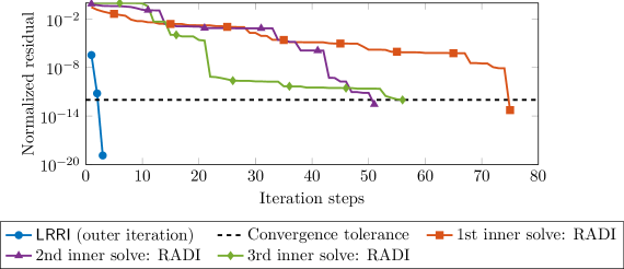
Figure 1: Convergence of Riccati iteration and inner solvers for the rail example.

As second example, we consider the laminar flow in a wake with a cylinder obstacle at Reynolds number $60$, as described in [16] and with the data available at [33]. The example has two inputs modeling the suction and injection of fluid at the back of the cylinder placed in the beginning of the wake. We consider the case that one of the outlets is defect and produces only noise that needs to be compensated. Therefor, the defect outlet gives us the $B_{1}$ matrix and the control outlet gives us the matrix $B_{2}$. Also, the considered Riccati equation has exactly the structure as in Eq. 12 resulting from the underlying dynamical system of differential-algebraic equations. Therefor, we use the implicit truncation approach mentioned in Section 2.4.2, which is implemented in the dae_2 function handles in [53]. Also, we note that the matrix pencil of this example has unstable eigenvalues. Since RADI is difficult to use for such a problem since it needs a stabilizing initial solution that produces a positive semi-definite residual in the Riccati operator, we switch only for the first iteration step of LRRI to the LR-Newton-ADI method and use a stabilizing Bernoulli feedback the same way as in [5]. The results of LRRI can be seen in the cylinderwake column of Table 5 and the normalized residuals of the outer and inner iterations are shown in Figure 2. While the relative residual is comfortably small again for this example due to the very large norm of the stabilizing solution, the normalized residual is still quite high. This likely comes from the general bad conditioning of the problem and the small norm of the right-hand side matrix. But overall, the computed solution has been obtained with reasonable accuracy and in a reasonable amount of time.

graphics/cylinderwake.tikzgraphics/externalize/cylinderwake.pdf

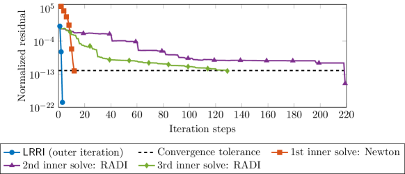
Figure 2: Convergence of Riccati iteration and inner solvers for the cylinder wake example.

4 Conclusions

We have developed a low-rank iterative method for solving large-scale sparse Riccati equations with indefinite quadratic terms, which is based on solutions of Riccati equations with negative semi-definite quadratic terms. Numerical examples have illustrated that, in the dense case, we can expect a similar accuracy and good performance in comparison to other established Riccati equation solvers, and that for large-scale sparse equations, the method also yields reasonably good results. We have also extended the LR-RI approach to indefinite algebraic Riccati equations related to descriptor systems with singular $E$ matrix.

To our knowledge, the low-rank Riccati iteration is currently the only approach to solve Riccati equations with indefinite quadratic terms in the large-scale sparse case. Another idea that might be directly extendable to this problem are projection-based methods. However, a problem occurring already in the case of classical Riccati equations with semi-definite quadratic terms is the solvability of the projected equations. Only recently, new results have been obtained under which conditions constructed projection spaces preserve the existence of stabilizing solutions in projected Riccati equations with negative semi-definite quadratic terms [63]. This problem becomes even more complicated when dealing with Riccati equations with indefinite quadratic terms, and so far, there are neither theoretical nor numerical results available considering this.

References

- [1] G. S. Ammar, P. Benner, and V. Mehrmann. A multishift algorithm for the numerical solution of algebraic Riccati equations. Electron. Trans. Numer. Anal., 1:33–48, 1993. URL: https://etna.math.kent.edu/volumes/1993-2000/vol1/abstract.php?vol=1&pages=33-48.
- [2] B. D. O. Anderson and J. B. Moore. Optimal Control: Linear Quadratic Methods. Prentice-Hall, Englewood Cliffs, NJ, 1990.
- [3] B. D. O. Anderson and B. Vongpanitlerd. Network Analysis and Synthesis: A Modern Systems Approach. Networks Series. Prentice-Hall, Englewood Cliffs, NJ, 1972.
- [4] W. F. Arnold and A. J. Laub. Generalized eigenproblem algorithms and software for algebraic Riccati equations. Proc. IEEE, 72(12):1746–1754, 1984. doi:10.1109/PROC.1984.13083.
- [5] E. Bänsch, P. Benner, J. Saak, and H. K. Weichelt. Riccati-based boundary feedback stabilization of incompressible Navier-Stokes flows. SIAM J. Sci. Comput., 37(2):A832–A858, 2015. doi:10.1137/140980016.
- [6] T. Başar and J. Moon. Riccati equations in Nash and Stackelberg differential and dynamic games. IFAC-PapersOnLine, 50(1):9547–9554, 2017. doi:10.1016/j.ifacol.2017.08.1625.
- [7] P. Benner. Contributions to the Numerical Solution of Algebraic Riccati Equations and Related Eigenvalue Problems. Dissertation, Department of Mathematics, TU Chemnitz-Zwickau, Chemnitz, Germany, 1997.
- [8] P. Benner. Numerical solution of special algebraic Riccati equations via an exact line search method. In 1997 European Control Conference (ECC), pages 3136–3141, 1997. doi:10.23919/ECC.1997.7082591.
- [9] P. Benner. Partial stabilization of descriptor systems using spectral projectors. In P. Van Dooren, S. P. Bhattacharyya, R. H. Chan, V. Olshevsky, and A. Routray, editors, Numerical Linear Algebra in Signals, Systems and Control, volume 80 of Lect. Notes Electr. Eng., pages 55–76. Springer, Dodrecht, 2011. doi:10.1007/978-94-007-0602-6_3.
- [10] P. Benner and Z. Bujanović. On the solution of large-scale algebraic Riccati equations by using low-dimensional invariant subspaces. Linear Algebra Appl., 488:430–459, 2016. doi:10.1016/j.laa.2015.09.027.
- [11] P. Benner, Z. Bujanović, P. Kürschner, and J. Saak. RADI: a low-rank ADI-type algorithm for large scale algebraic Riccati equations. Numer. Math., 138(2):301–330, 2018. doi:10.1007/s00211-017-0907-5.
- [12] P. Benner, Z. Bujanović, P. Kürschner, and J. Saak. A numerical comparison of different solvers for large-scale, continuous-time algebraic Riccati equations and LQR problems. SIAM J. Sci. Comput., 42(2):A957–A996, 2020. doi:10.1137/18M1220960.
- [13] P. Benner, P. Ezzatti, Quintana-Ortí E. S., and A. Remón. A factored variant of the Newton iteration for the solution of algebraic Riccati equations via the matrix sign function. Numer. Algorithms, 66(2):363–377, 2014. doi:10.1007/s11075-013-9739-2.
- [14] P. Benner and J. Heiland. Nonlinear feedback stabilization of incompressible flows via updated Riccati-based gains. In 2017 IEEE 56th Annual Conference on Decision and Control (CDC), pages 1163–1168, 2017. doi:10.1109/CDC.2017.8263813.
- [15] P. Benner and J. Heiland. Equivalence of Riccati-based robust controller design for index-1 descriptor systems and standard plants with feedthrough. In 2020 European Control Conference (ECC), pages 402–407, 2020. doi:10.23919/ECC51009.2020.9143771.
- [16] P. Benner, J. Heiland, and S. W. R. Werner. Robust output-feedback stabilization for incompressible flows using low-dimensional -controllers. e-print 2103.01608, arXiv, 2021. math.OC. URL: https://arxiv.org/abs/2103.01608.
- [17] P. Benner, M. Köhler, and J. Saak. Matrix equations, sparse solvers: M-M.E.S.S.-2.0.1—Philosophy, features and application for (parametric) model order reduction. In P. Benner, T. Breiten, H. Faßbender, M. Hinze, T. Stykel, and R. Zimmermann, editors, Model Reduction of Complex Dynamical Systems, volume 171 of International Series of Numerical Mathematics, pages 369–392. Birkhäuser, Cham, 2021. doi:10.1007/978-3-030-72983-7_18.
- [18] P. Benner, P. Kürschner, and J. Saak. A reformulated low-rank ADI iteration with explicit residual factors. Proc. Appl. Math. Mech., 13(1):585–586, 2013. doi:10.1002/pamm.201310273.
- [19] P. Benner, P. Kürschner, and J. Saak. Self-generating and efficient shift parameters in ADI methods for large Lyapunov and Sylvester equations. Electron. Trans. Numer. Anal., 43:142–162, 2014. URL: https://etna.mcs.kent.edu/volumes/2011-2020/vol43/abstract.php?vol=43&pages=142-162.
- [20] P. Benner, J.-R. Li, and T. Penzl. Numerical solution of large-scale Lyapunov equations, Riccati equations, and linear-quadratic optimal control problems. Numer. Lin. Alg. Appl., 15(9):755–777, 2008. doi:10.1002/nla.622.
- [21] P. Benner and J. Saak. Numerical solution of large and sparse continuous time algebraic matrix Riccati and Lyapunov equations: a state of the art survey. GAMM-Mitt., 36(1):32–52, 2013. doi:10.1002/gamm.201310003.
- [22] P. Benner and T. Stykel. Numerical solution of projected algebraic Riccati equations. SIAM J. Numer. Anal., 52(2):581–600, 2014. doi:10.1137/130923993.
- [23] P. Benner and T. Stykel. Model order reduction for differential-algebraic equations: A survey. In A. Ilchmann and T. Reis, editors, Surveys in Differential-Algebraic Equations IV, Differential-Algebraic Equations Forum, pages 107–160. Springer, Cham, 2017. doi:10.1007/978-3-319-46618-7_3.
- [24] P. Benner and S. W. R. Werner. Model reduction of descriptor systems with the MORLAB toolbox. IFAC-PapersOnLine, 51(2):547–552, 2018. doi:10.1016/j.ifacol.2018.03.092.
- [25] P. Benner and S. W. R. Werner. MORLAB – Model Order Reduction LABoratory (version 5.0), August 2019. See also: https://www.mpi-magdeburg.mpg.de/projects/morlab. doi:10.5281/zenodo.3332716.
- [26] P. Benner and S. W. R. Werner. MORLAB—The Model Order Reduction LABoratory. In P. Benner, T. Breiten, H. Faßbender, M. Hinze, T. Stykel, and R. Zimmermann, editors, Model Reduction of Complex Dynamical Systems, volume 171 of International Series of Numerical Mathematics, pages 393–415. Birkhäuser, Cham, 2021. doi:10.1007/978-3-030-72983-7_19.
- [27] M. C. Delfour. Linear quadratic differential games: Saddle point and Riccati differential equation. SIAM J. Control Optim., 46(2):750–774, 2007. doi:10.1137/050639089.
- [28] U. B. Desai and D. Pal. A realization approach to stochastic model reduction and balanced stochastic realizations. In 21st IEEE Conference on Decision and Control, pages 1105–1112, 1982. doi:10.1109/CDC.1982.268322.
- [29] J. Doyle, K. Glover, P. P. Khargonekar, and B. A. Francis. State-space solutions to standard and control problems. IEEE Trans. Autom. Control, 34(8):831–847, 1989. doi:10.1109/9.29425.
- [30] F. Freitas, J. Rommes, and N. Martins. Gramian-based reduction method applied to large sparse power system descriptor models. IEEE Trans. Power Syst., 23(3):1258–1270, 2008. doi:10.1109/TPWRS.2008.926693.
- [31] G. H. Golub and C. F. Van Loan. Matrix Computations. Johns Hopkins Studies in the Mathematical Sciences. Johns Hopkins University Press, Baltimore, fourth edition, 2013.
- [32] J. Heiland. A differential-algebraic Riccati equation for applications in flow control. SIAM J. Control Optim., 54(2):718–739, 2016. doi:10.1137/151004963.
- [33] J. Heiland and S. W. R. Werner. Code, data and results for numerical experiments in “Robust output-feedback stabilization for incompressible flows using low-dimensional -controllers” (version 2.0), October 2021. doi:10.5281/zenodo.5532539.
- [34] M. Heinkenschloss, D. C. Sorensen, and K. Sun. Balanced truncation model reduction for a class of descriptor systems with application to the Oseen equations. SIAM J. Sci. Comput., 30(2):1038–1063, 2008. doi:10.1137/070681910.
- [35] M. Heyouni and K. Jbilou. An extended block Arnoldi algorithm for large-scale solutions of the continuous-time algebraic Riccati equation. Electron. Trans. Numer. Anal., 33:53–62, 2009. URL: https://etna.math.kent.edu/volumes/2001-2010/vol33/abstract.php?vol=33&pages=53-62.
- [36] E. A. Jonckheere and L. M. Silverman. A new set of invariants for linear systems–application to reduced order compensator design. IEEE Trans. Autom. Control, 28(10):953–964, 1983. doi:10.1109/TAC.1983.1103159.
- [37] D. L. Kleinman. On an iterative technique for Riccati equation computations. IEEE Trans. Autom. Control, 13(1):114–115, 1968. doi:10.1109/TAC.1968.1098829.
- [38] P. Kürschner. Efficient Low-Rank Solution of Large-Scale Matrix Equations. Dissertation, Department of Mathematics, Otto von Guericke University, Magdeburg, Germany, 2016. URL: http://hdl.handle.net/11858/00-001M-0000-0029-CE18-2.
- [39] P. Lancaster and L. Rodman. Algebraic Riccati Equations. Oxford Science Publications. The Clarendon Press, Oxford University Press, New York, 1995.
- [40] A. Lanzon, Y. Feng, and B. D. O. Anderson. An iterative algorithm to solve algebraic Riccati equations with an indefinite quadratic term. In 2007 European Control Conference (ECC), pages 3033–3039, 2007. doi:10.23919/ecc.2007.7068239.
- [41] A. Lanzon, Y. Feng, B. D. .O. Anderson, and M. Rotkowitz. Computing the positive stabilizing solution to algebraic Riccati equations with an indefinite quadratic term via a recursive method. IEEE Trans. Autom. Control, 53(10):2280–2291, 2008. doi:10.1109/TAC.2008.2006108.
- [42] A. J. Laub. A Schur method for solving algebraic Riccati equations. IEEE Trans. Autom. Control, 24(6):913–921, 1979. doi:10.1109/TAC.1979.1102178.
- [43] F. Leibfritz. : COnstrained Matrix-optimization Problem library – a collection of test examples for nonlinear semidefinite programs, control system design and related problems. Tech.-report, University of Trier, 2004. URL: http://www.friedemann-leibfritz.de/COMPlib_Data/COMPlib_Main_Paper.pdf.
- [44] J.-R. Li and J. White. Low rank solution of Lyapunov equations. SIAM J. Matrix Anal. Appl., 24(1):260–280, 2002. doi:10.1137/S0895479801384937.
- [45] Y. Lin and V. Simoncini. A new subspace iteration method for the algebraic Riccati equation. Numer. Linear Algebra Appl., 22(1):26–47, 2015. doi:10.1002/nla.1936.
- [46] A. Locatelli. Optimal Control: An Introduction. Birkhäuser, Basel, 2001.
- [47] D. C. McFarlane and K. Glover. Robust Controller Design Using Normalized Coprime Factor Plant Descriptions, volume 138 of Lect. Notes Control Inf. Sci. Springer, Berlin, Heidelberg, 1990. doi:10.1007/BFB0043199.
- [48] J. Möckel, T. Reis, and T. Stykel. Linear-quadratic Gaussian balancing for model reduction of differential-algebraic systems. Internat. J. Control, 84(10):1627–1643, 2011. doi:10.1080/00207179.2011.622791.
- [49] D. Mustafa and K. Glover. Controller reduction by -balanced truncation. IEEE Trans. Autom. Control, 36(6):668–682, 1991. doi:10.1109/9.86941.
- [50] P. C. Opdenacker and E. A. Jonckheere. A contraction mapping preserving balanced reduction scheme and its infinity norm error bounds. IEEE Trans. Circuits Syst., 35(2):184–189, 1988. doi:10.1109/31.1720.
- [51] J. D. Roberts. Linear model reduction and solution of the algebraic Riccati equation by use of the sign function. Internat. J. Control, 32(4):677–687, 1980. Reprint of Technical Report No. TR-13, CUED/B-Control, Cambridge University, Engineering Department, 1971. doi:10.1080/00207178008922881.
- [52] J. Saak. Efficient Numerical Solution of Large Scale Algebraic Matrix Equations in PDE Control and Model Order Reduction. Dissertation, Department of Mathematics, University of Technology Chemnitz, Chemnitz, Germany, 2009. URL: https://nbn-resolving.org/urn:nbn:de:bsz:ch1-200901642.
- [53] J. Saak, M. Köhler, and P. Benner. M-M.E.S.S. – The Matrix Equations Sparse Solvers library (version 2.1), April 2021. See also: https://www.mpi-magdeburg.mpg.de/projects/mess. doi:10.5281/zenodo.4719688.
- [54] J. Saak and M. Voigt. Model reduction of constrained mechanical systems in M-M.E.S.S. IFAC-PapersOnLine, 51(2):661–666, 2018. doi:10.1016/j.ifacol.2018.03.112.
- [55] N. Sandell. On Newton’s method for Riccati equation solution. IEEE Trans. Autom. Control, 19(3):254–255, 1974. doi:10.1109/TAC.1974.1100536.
- [56] V. Simoncini. Analysis of the rational Krylov subspace projection method for large-scale algebraic Riccati equations. SIAM J. Matrix Anal. Appl., 37(4):1655–1674, 2016. doi:10.1137/16M1059382.
- [57] E. D. Sontag. Mathematical Control Theory, volume 6 of Texts in Applied Mathematics. Springer, New York, second edition, 1998.
- [58] T. Stillfjord. Singular value decay of operator-valued differential Lyapunov and Riccati equations. SIAM J. Control Optim., 56(5):3598–3618, 2018. doi:10.1137/18M1178815.
- [59] T. Stykel. Analysis and Numerical Solution of Generalized Lyapunov Equations. Dissertation, Faculty II – Mathematics and Nature Sciences, Technische Universität Berlin, Berlin, Germany, 2002. doi:10.14279/depositonce-578.
- [60] T. Stykel. Low-rank iterative methods for projected generalized Lyapunov equations. Electron. Trans. Numer. Anal., 30:187–202, 2008. URL: https://etna.math.kent.edu/volumes/2001-2010/vol30/abstract.php?vol=30&pages=187-202.
- [61] A. Varga. On computing high accuracy solutions of a class of Riccati equations. Control–Theory and Advanced Technology, 10(4):2005–2016, 1995.
- [62] H. K. Weichelt. Numerical Aspects of Flow Stabilization by Riccati Feedback. Dissertation, Department of Mathematics, Otto von Guericke University, Magdeburg, Germany, 2016. doi:10.25673/4493.
- [63] L. Zhang, H.-Y. Fan, and E. K. Chu. Inheritance properties of Krylov subspace methods for continuous-time algebraic Riccati equations. J. Comput. Appl. Math., 371:112685, 2020. doi:10.1016/j.cam.2019.112685.