Supersonic Expansion of the Bipolar Hii Region Sh2-106: A 3,500 Year-Old Explosion?

Abstract

Multi-epoch narrow-band HST images of the bipolar Hii region Sh2-106 reveal highly supersonic nebular proper motions which increase with projected distance from the massive young stellar object S106 IR, reaching over $\sim$30 mas yr^-1 ($\sim$150 km s^-1 at D=1.09 kpc) at a projected separation of $\sim$1.4′ (0.44 pc) from S106 IR. We propose that S106 IR experienced a $\sim 10^{47}$ erg explosion $\sim$3,500 years ago. The explosion may be the result of a major accretion burst, a recent encounter with another star, or a consequence of the interaction of a companion with the bloated photosphere of S106 IR as it grew from $\sim$10 through $\sim 15$ M_⊙  at a high accretion rate. Near-IR images reveal fingers of H₂ emission pointing away from S106 IR and an asymmetric photon-dominated region surrounding the ionized nebula. Radio continuum and Br-$\gamma$ emission reveal a C-shaped bend in the plasma, either indicating motion of S106 IR toward the east, or deflection of plasma toward the west by the surrounding cloud. The Hii region bends around a $\sim$1′ diameter dark bay west of S106 IR that may be shielded from direct illumination by a dense molecular clump. Herbig-Haro (HH) and Molecular Hydrogen Objects (MHOs) tracing outflows powered by stars in the Sh2-106 proto-cluster such as the Class 0 source S106 FIR are discussed.

1 Introduction

The birth and early evolution of massive stars remain one of the least understood aspects of star formation. Massive stars play essential roles in the feedback and self-regulation of star formation and profoundly impact the environments in which lower mass sibling stars and their planetary systems form (Krumholz, Klein & McKee, 2011, 2012; Krumholz, et al., 2014; Dale et al., 2012, 2014; Federrath et al., 2014). The nearest region of on-going massive star formation, Orion OMC1, experienced a powerful explosion about 550 years ago (Bally & Zinnecker, 2005; Zapata et al., 2009; Bally et al., 2015, 2017, 2020). Several other massive star forming regions contain explosive protostellar outflows (Zapata et al., 2017, 2020). Here we show that the exciting star of the Hii region Sh2-106 (S106 for short) likely experienced a powerful explosion several thousands of years ago.

The gravitational collapse of molecular clouds drives the formation of clumps and protostellar cores, which undergo inside-out collapse to form young stellar objects (YSOs). The infalling flow’s angular momentum leads to the formation of circumstellar disks in which viscous dissipation fuels further accretion onto the YSO. Shear amplification of entrained magnetic fields and convection-powered magneto-hydrodynamic (MHD) dynamos can drive winds and collimated jets, which entrain matter from the surrounding cloud to produce bipolar molecular outflows (Pudritz & Ray, 2019). Thus, most stars produce bipolar outflows as they accrete from their parent clouds and grow in mass (Bally, 2016).

These protostellar outflows are a potent source of feedback in the self-regulation of star formation because they inject momentum and kinetic energy into their host clouds efficiently. Outflows create turbulence, dissociate molecules, and can disrupt the star-formation environment. Outflow momentum and kinetic energy injection rates increase with protostellar luminosity and mass. Thus, as forming massive stars accrete from their parent clouds and cores, they usually drive the most powerful molecular outflows in their environment. Hence, in a forming cluster of stars, the most massive young stellar object (MYSO) tends to have the greatest feedback impact on the parent cloud (Maud et al., 2015a, b; Bally, 2016).

Most MYSOs form as parts of multiple star systems inside clusters, typically containing hundreds of lower mass YSOs (Zinnecker & Yorke, 2007). Multiplicity and surrounding cluster members can dramatically alter the evolution of MYSOs (Peters et al., 2010a, b, c). Multi-body interactions with sibling stars can re-orient accretion disks and alter outflow orientations (Cunningham, Moeckel, & Bally, 2009; Bally, 2016). Compact, non-hierarchical multiple systems, binary-binary, and N-body interactions can eject cluster members (Reipurth et al., 2010; Reipurth & Mikkola, 2012, 2015). Such interactions can lead to protostellar mergers and explosive outflows such as in Orion OMC1 located behind the Orion Nebula (Bally et al., 2015, 2017, 2020). Although several other explosive outflows have been identified such as DR21 (Zapata et al., 2013) and G5.89-0.39 (Zapata et al., 2020), the event rate of protostellar explosions is not yet known. Thus, it is important to identify additional examples to constrain the event rate.

MYSO cores rapidly reach the main-sequence (Zinnecker & Yorke, 2007). However, their envelopes become bloated in the presence of high-accretion rates. Photospheric radii can grow to 1 AU or more as their masses reach $\sim$10 M_⊙. Thus, rapidly accreting MYSOs ($\dot{M}>10^{-4}$ M_⊙yr ^-1) have low effective temperatures resembling post-main-sequence supergiant stars (Hosokawa & Omukai, 2009). As MYSOs grow beyond 15 M_⊙ and accretion subsides, they eventually shrink in radius and become hot O-stars, emitting hydrogen-ionizing Lyman continuum (LyC) radiation. This radiation dissociates, heats, and ionizes a bubble, including the bipolar molecular outflow generated during its main accretion phase. Such feedback can halt star-formation by blowing out the gas supply fueling the growth of the MYSO and that of other stars. In areas where the sound speed in the photo-ionized gas, typically around 10 km s^-1, is larger than the gravitational escape speed, the plasma can be expelled from the parent cloud. Such feedback can lead to the cloud’s destruction (e.g. Bressert et al. 2012).

Massive, main-sequence stars power stellar winds with speeds up to several thousand kilometers per second and mass-loss rates of the order $\dot{M}\sim 10^{-8}$ to over $10^{-6}$ M_⊙ yr^-1 (Puls et al., 2008). Such winds create hot, X-ray-bright bubbles of million-Kelvin plasma surrounded by swept-up shells of cooler material. During the early phases of stellar-wind bubble evolution, the ram pressure of the wind is converted to thermal pressure in a reverse-shock. Expansion of the hot bubble sweeps-up the surrounding Hii region into a shell in an energy-conserving interaction. At later times, when radiative and conductive cooling of the hot bubble becomes dominant, this ram-pressure continues to drive the shell in a momentum conserving interaction (Castor, McCray & Weaver, 1975; Weaver, et al., 1977; Geen et al., 2020a, b).

Some forming MYSOs such as S106 IR drive winds with much slower speeds but higher mass-loss rates than main-sequence stars (Simon et al., 1983; Jaffe & Martín-Pintado, 1999). The dense plasma near the base of the wind produces strong near- and mid-IR hydrogen recombination lines; free-free continuum emission at radio frequencies originates farther from the star. Such winds are seen as compact radio sources at the location of the MYSO. For a constant velocity and constant mass-loss-rate wind or jet that spreads with a constant opening angle, the electron density decreases as $r^{-2}$. Because the wind photospheric radius (where the free-free optical depth $\sim$1) shrinks with increasing frequency, the flux-density of such winds increase roughly as $\nu^{0.7}$ (Simon & Fischer, 1982; Simon et al., 1983; Bally, Snell & Predmore, 1983).

S106 provides a unique opportunity to study the short-lived transition from massive protostar to a main-sequence star surrounded by an emerging Hii  region. Of particular interest in this transition is the nature of the feedback mechanisms that halt accretion and destroys the parent cloud. S106 provides a unique nearby laboratory in which to study the transition from outflow driven feedback to UV and wind-powered feedback in the destruction of the parent molecular cloud and emergence of a young cluster surrounding an O star.

In this paper, we present an analysis of nebular proper motions based on multi-epoch Hubble Space Telescope (HST) images taken with an interval of 16 years. The images were registered using field stars whose positions were determined during the epoch of each HST observation using proper motions measured by the Gaia satellite and presented in Gaia EDR3. The nebular proper motions increase linearly with projected distance from S106 IR, reaching speeds of order 150 km s^-1 at the outer edge of the ionized nebula. The nature of the supersonic expansion and what it implies for the evolutionary stage of S106 is discussed.

We present narrow-band images of S106 in the 2.12 $\mu$m S(1) emission line of H₂ and the 2.16 $\mu$m Brackett-$\gamma$ hydrogen recombination emission line. The H₂ emission shows the photon-dominated region’s structure (PDR) surrounding the Hii region. These images reveal fingers of H₂ emission pointing directly away from S106 IR and knots of H₂ emission beyond the PDR that may trace debris ejected by S106 IR and/or shocks powered by protostellar outflows from lower-mass protostars in the S106 cluster. The Br-$\gamma$ emission line shows that the plasma in S106 exhibits C-shaped symmetry with the northern and southern lobes deflected towards the west. The ends of each nebular lobe are capped by ‘bright-bars’ of emission about 80″ from S106 IR.

Section 2 presents an overview of S106. Section 3 describes the data sets presented here. Section 4 describes the reduction and registration of images and the nebular proper motion measurements. Section 5 presents new near-IR images. Section 6 combines the proper motion analysis, IR-images, with results from the literature to interpret the physics of S106. Section 7 presents a summary. Additional images and figures showing features discussed in the text are presented in Appendices.

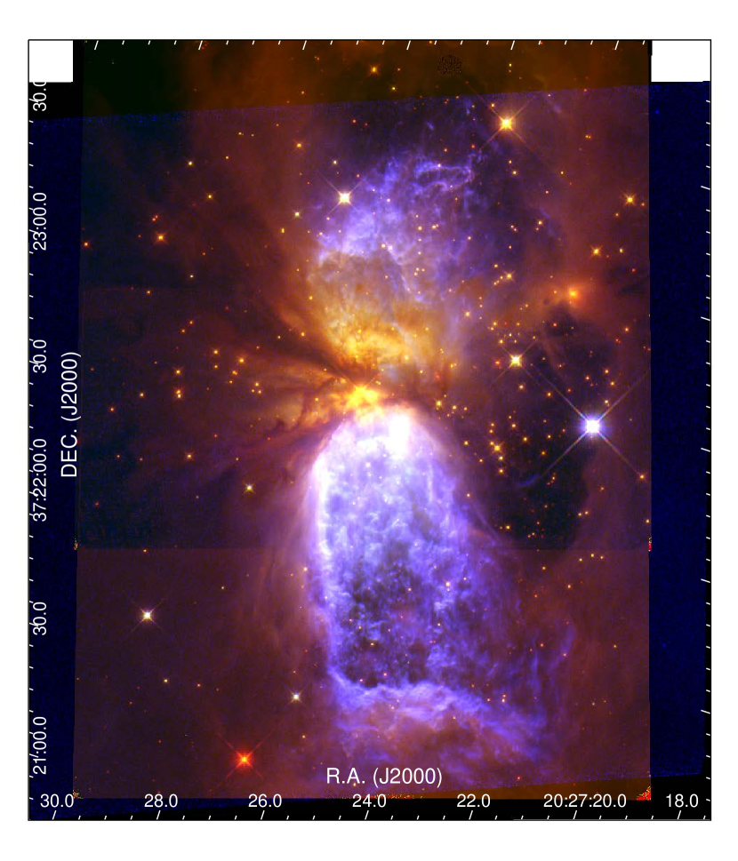
Figure 1: An HST image showing S106 in the H-band F160W filter at 1.6 $\mu$m (red), the J-band F110W filter at 1.1 $\mu$m (green), and a narrow-band F658N filter transmitting [Nii] (blue) using data obtained in 2011. The image was rotated so north is 18^o to the right of vertical. The vertical extent of this image is 186″ (0.98 pc).

2 Overview of S106

S106 is the nearest bipolar Hii region, a subclass of very young photo-ionized nebulae, in which a nearly edge-on disk or belt of dense material splits the ionized nebula into a pair of lobes (Eiroa et al., 1979; Neckel, 1982). Long-slit spectroscopy demonstrated that H$\alpha$ exhibits supersonic expansion away from the central ionizing source (Solf, 1980). S106 is ionized by a highly obscured late-O star known as S106 IR embedded in the dark lane (Hodapp & Schneider, 2008). Figure 1 shows an HST image of S106 obtained in the broad-band 1.1 $\mu$m and 1.6 $\mu$m filters F110W and F160W with WFC3 on HST. Figure 2 shows a narrow-band 6584Å [Nii] image acquired with the F658N filter in WFC3.

S106 is located in the Cygnus-X region at Galactic coordinates $l$=76.4^o $b$=$-$0.6^o where radial velocities provide an unreliable measure of distance. Thus, distance estimates have ranged from $\sim$500 pc to $\sim$5.7 kpc (for a review, see Hodapp & Schneider 2008). Parallax measurements at radio wavelengths towards the 22 GHz H₂O maser from the Class 0 source S106 FIR (Furuya et al., 1999, 2000) give a distance of $\sim$1.3$\pm 0.1$ kpc (Xu et al., 2013). The most reliable estimate uses the Gaia DR2 distances to dozens of stars toward the S106 molecular cloud that lie either in front or behind the cloud. The parallax at which the extinction and reddening increase abruptly (in a so-called ‘Wolf’ plot named after Max Wolf, who pioneered the method about a century ago) gives a distance of 1,091$\pm$54 pc (Zucker et al., 2020). In this paper, we adopt a distance of 1.09 kpc.

S106 is a young Hii region whose central star is in the late stages of formation and still embedded in a cometary molecular cloud (Bally & Scoville, 1982; Schneider et al., 2002). Schneider et al. (2002) found a total mass of $\sim$2,000 M_⊙ for the cloud using ¹³CO and assuming a distance of 600 pc. Scaling this to our adopted distance of 1.09 kpc implies a total mass of $\sim$6,600 M_⊙. S106 contains a cluster of $\sim$600 young stellar object, including a substantial number of sub-stellar objects with an age less than 1 Myr (Oasa et al., 2006).

Israel & Felli (1978) measured the total radio continuum flux from S106 at 1.4 and 5 GHz finding an approximately flat spectral index with a total flux density of S_1.4 = 11.1 Jy and S₅ = 12.3 Jy indicating optically thin free-free emission. For their assumed distance of 3.6 kpc, Israel & Felli (1978) derived a total Hii region mass of 35 M_⊙. Scaling this to 1.09 kpc implies a total plasma mass of 3.1 M_⊙.

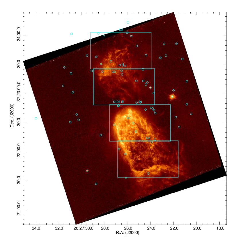
Figure 2: An HST WFC3 image showing S106 in the narrow-band [Nii] filter F658N that excludes the H$\alpha$ emission line. This image was obtained in 2011. Boxes mark the locations of the four sub-frames shown in Appendices A and B. Cyan circles mark the locations of stars for which Gaia EDR3 provides proper motions. The stellar proper motions were traced back from the 2015.5 reference date to the dates on which the 1995 and 2011 images were acquired. The computed positions of these stars at the time the images were taken were used to register the images.

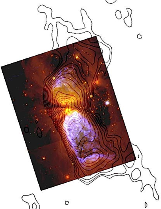
Figure 3: Contours of 4.8 GHz radio continuum emission superimposed on a color image of S106 showing 1.6 $\mu$m (red), 1.1 $\mu$m (green), and 0.6584 $\mu$m [Nii] emission. Note the C-shaped bend and the presence of bars of enhanced free-free emission located at south end of the southern lobe and the north end of the northern lobe (for a clearer view of the South Bar and Northwest Bar, see Figure 6. The beam diameter is 10″. Contour levels are at 13.4, 26.7, 40.1, 53.5, 66.9, 80.2, 93.6, 107.0, 120, 134, 267, 401, 535, 669, 802, 936, 1070, 1204, and 1337 mJy/beam. The peak flux is 1.337 Jy/beam. The figure is aligned with north along the vertical axis.

The southern lobe of S106 is much brighter than the northern lobe at visual-wavelengths. However, at centimeter wavelengths, the northern lobe has similar intensity and size to the southern lobe, indicating that the northern lobe is hidden by more extinction than the southern lobe (Figure 3). The radio data shows the bright features evident in the mid-infrared within 30″ of S106 IR. The bright bar seen at visual and near-IR wavelengths located 1.2′ south of S106 IR is also a prominent radio continuum emission feature.

The dark equatorial band in Figure 1 is also present in high-resolution radio images (Bally, Snell & Predmore, 1983). Thus, this feature is not merely caused by foreground obscuration. Rather, it traces a lack of plasma due to the presence of either dense atomic or molecular gas. This region may be shadowed by a compact disk. Barsony et al. (1989) presented interferometric observations of ¹³CO, CS, and HCN but failed to find evidence of a massive disk. Dense gas was found to be concentrated in two peaks along the eastern and western walls of the Hii region with a bridge of emission connecting the peaks at the location of the equatorial dark region.

From near-IR to sub-mm wavelengths, S106 has a dust luminosity $L_{dust}>9\times 10^{4}$ L_⊙ (Adams et al., 2015). The dust temperature decreases with increasing distance from S106 IR, indicating that this star is the primary heating source. Mid-IR ($\lambda\sim$3.6 to 12 $\mu$m) images show several fingers of dust in absorption, converging on the position of S106 IR, which is a bright point source at these wavelengths. In the Herschel 70 and 160 $\mu$m images, these dust streamers are seen in emission and may trace streamers of dense gas falling into the equatorial region of S106 (Adams et al., 2015; Schneider, et al., 2018).

High-resolution visual-wavelength spectroscopy of H$\alpha$, [Nii], and [Sii] (Solf & Carsenty, 1982) shows that the northern lobe of S106 is redshifted with a mean velocity of V_LSR$\approx$22 km s^-1. Within a half-arcminute of S106 IR, the line-widths are $\sim$45 km s^-1 at half-maximum and up to $\sim$120 km s^-1 at zero intensity. The H$\alpha$ profile towards the southern lobe shows line-splitting with two components separated by up to 100 km s^-1  within 30″ of S106 IR; most of this emission is blue-shifted. Beyond 30″ from S106 IR, the brighter southern lobe has a slight blueshift of about V_LSR$\approx-$12 km s^-1 along with some gas close to V_LSR= 0 km s^-1. Noel et al. (2005) presented near-IR Fourier Transform Spectroscopy of H₂, Hei, Br-$\gamma$, and [Fe iii] of the inner region of S106 within 30″ of S106 IR, finding that Br-$\gamma$ exhibits emission over a velocity range of $-$45 to +80 km s^-1.

The Hii region sits inside a roughly cylindrical, $\sim$6′  (1.9 pc) long cavity bounded by warm dust and PAH emission at 3.6 to 8.0 $\mu$m (see Appendix C for more discussion). This cavity is more than a factor of two longer and wider than the Hii region at visual, near-IR, and radio wavelengths. S106 IR is displaced from the center of this cavity and located near its eastern edge.

Schneider et al. (2003) presented an extensive FIR sub-mm study of S106, finding strong C⁺, [Oi], and high-J emission from CO and a variety of dense gas tracers commonly associated with PDRs in intense UV radiation fields. Schneider et al. (2007) found blue-shifted CO emission from the southern lobe of S106, red-shifted emission towards the northern lobe, and interpreted these features as tracing part of a bipolar flow from S106 IR. The S106 molecular cloud is cometary with the S106 Hii region located in the dense head of the cloud at its northern edge. This indicates that feedback from several Cygnus-X OB clusters, especially NGC 6913, located north of S106 have shaped this cloud (Schneider et al., 2007).

Simon et al. (2012) mapped the 158 $\mu$m C⁺, CO J=11$-$10, and 350 $\mu$m dust continuum emission with high spectral resolution and $\sim$6″ angular resolution, finding complex morphology and kinematics. These tracers identify a belt of warm, high-velocity gas extending from the eastern rim of the Hii region to S106 FIR, closely following the northern portion of the dark lane (Figures 1 and 2). Remarkably, the C⁺ emission towards the southern lobe close to S106 IR is red-shifted (Simon et al., 2012), opposite to the radial velocity of the H$\alpha$ emission. It appears that the front-side of the southern cavity has been eroded, and most of the visual-wavelength emission likely originates from the rear wall of the cavity, with the C⁺ emission originating in a PDR behind the ionization front at a somewhat higher radial velocity than the H$\alpha$ emission, especially near S106 IR (Schneider, et al., 2018). Schneider, et al. (2018) show a cartoon of the suspected geometry.

2.1 The young O-star, S106 IR

S106 IR is a binary with an orbital period of $\sim$5 days, a semimajor axis of 0.17 AU, and eccentricity of $\sim$0.2. The primary is a $\sim$20 M_⊙ O8 or O9 star; the secondary is a $\sim$3 M_⊙ B8 star (Comerón et al., 2018). The binary exhibits short-term (hours time-scale) photometric variability whose intensity peaks around the time of periastron, possibly indicating accretion bursts.

Beuther et al. (2018) used the NOEMA interferometer to show that S106 IR is surrounded by a massive disk or core with a mass of about 1 M_⊙ and an outer radius of about 800 AU using a distance of 1.3 kpc. This corresponds to a mass of $\sim$0.7 M_⊙ and a radius $\sim$650 AU at a distance of 1.09 kpc. Beuther et al. (2018) also found a $\sim$0.03 M_⊙ core (scaled to D$\sim$1.09 kpc) 4″ northeast of S106 IR in the dust lane connecting the east side of S106 to S106 IR.

Bally, Snell & Predmore (1983) found that S106 IR is an unresolved, point radio source at centimeter wavelengths in high-resolution VLA observations. It has a spectral index $S_{\nu}$ rising as $\nu^{0.7}$ between 5 and 22 GHz, indicating that the radio emission is produced by an ionized stellar wind or an outflow with a density profile decreasing with distance as $r^{-2}$. Gibb & Hoare (2007) found that the radio continuum emission at 22 GHz with 0.03″ resolution takes the shape of a torus surrounding S106 IR. It is elongated and measures $\sim$20 by 60 AU in extent, with its major axis aligned along the equatorial dark band seen in the radio, infrared, and visual wavelength images.

Gibb & Hoare (2007) interpreted this feature as a dense, equatorial wind which may be responsible for shielding the dense gas in the dark lane from ionizing radiation. This wind must be sufficiently enhanced in the equatorial direction to absorb the Lyman continuum. However, it must be optically thin to Lyman continuum along its polar axis in order to ionize the S106 Hii region. Lumsden et al. (2012) found spectroscopic evidence for such a wind which may be responsible for shadowing the dark lane. Such an equatorially enhanced wind may trace the ionized surface of a dense accretion disk.

The full-width-half-maxima (FWHM) of the Brackett 12, Brackett-$\gamma$ , and [Fe ii] line profiles range from 185 to 280 km s^-1. The wind-velocity of $\sim$200 km s^-1 (Simon & Fischer, 1982; Lumsden et al., 2012) combined with the radio spectral index of $\nu^{0.7}$ implies a mass-loss rate from S106 IR of about $10^{-6}$ M_⊙  yr^-1. More precise wind velocity measurements by Drew, Bunn, & Hoare (1993) found a mass-loss rate of at least $\dot{M}>2.7\times 10^{-6}$ M_⊙ yr^-1 and a wind velocity at infinity of at least 340 km s^-1. The slow wind velocity, and large mass-loss rate from S106 IR is unusual for a main sequence late-O star. Most O stars power winds with mass-loss rates around $10^{-8}$ to $10^{-7}$ M_⊙  yr^-1 and terminal velocities $\sim 10^{3}$ km s^-1 (Puls et al., 2008) . However, winds with parameters similar to the wind from S106 IR are found to be produced by some other massive young stellar objects (Simon et al., 1983).

The presence of a 0.7 M_⊙ compact ($\sim$ 700 AU) core inferred from the NOEMA 1.3 mm observations of S106 IR combined with the high resolution 22 GHz image suggest that a dense neutral disk surrounds S106 IR whose surface is ionized within 30 AU of S106 IR. The broad line profiles of the near-IR emission lines from S106 IR, such as Br-$\gamma$  may be produced by the Keplerian rotation of the photo-ionized disk surface. If the central mass is 23 M_⊙, the Kepler speed at 30 AU is 26 km s^-1; The Kepler speed at 1 AU is 143 km s^-1. The rising radio spectral index seen at centimeter-wavelengths indicates a dense wind. Such winds could be driven either by the central O-star, or by magneto-centrifugal processes at the disk surface, or a combination of the two mechanisms.

Murakawa et al. (2013) used adaptive-optics-assisted integral-field spectroscopy and spectro-astrometry to study S106 IR. They found evidence for a rotating, wide-angle, disk-wind emerging from the inner $\sim$0.43 AU portion of an edge-on disk (scaled to our assumed 1.09 kpc distance from their assumed 1.7 kpc distance) in Br$\gamma$ and CO overtone emission at 2.3 $\mu$m. The major axis of the disk has an orientation $\approx$100^o to 119^o, approximately at right-angles to the major axis of the bipolar Hii region. Modeling the $\pm$200 km s^-1 velocity difference on opposite sides of S106 IR as Keplerian rotation at a radius of $\sim$0.43 AU around S106 IR in a disk inclined by 83^o implies an enclosed mass of 19$\pm$4 M_⊙ (Murakawa et al., 2013) .

3 The Data Sets

3.1 Archival Data

The proper motion analysis presented here is based on narrow-band HST images acquired in 1995 and 2011. S106 was observed by HST in 1995 under GO program 5963 (Bally et a., 1998) targeting H$\alpha$  with WFPC2 using filter F656N. S106 was observed again by HST in 2011 targeting the [Nii] 6584Å emission line with WFC3 using filter F658N (GO program 12326: PI Keith Noll). In this program, images were also obtained in HeII 4686Å, [Oiii] 5007Å emission lines and the 1.1 and 1.6 $\mu$m continuum using the wide-band filters F110W and F160W. The observations used in the present analysis are summarized in Table 1. The time interval between the observations of the northern lobe of S106 in 1995 and the 2011 images was $\sim$15.578 years. For the southern lobe, the time interval was 15.124 years.

The far-infrared images presented here were obtained with the Spitzer Space Telescope and downloaded from the public archive at IPAC. The Sub-mm images were obtained with the Herschel Space Observatory under the Hi-GAL program. (Molinari et al., 2010a, b, 2016).

3.2 H₂, Br-$\gamma$, H$\alpha$, and 4.8 GHz Radio Observations

Narrow-band near-infrared images presented here were obtained using the Apache Point Observatory (APO) 3.5 meter telescope with the NICFPS camera on the dates indicated in Table 2. NICFPS uses a 1024 $\times$ 1024 pixel Rockwell Hawaii 1-RG HgCdTe detector. The pixel scale of this instrument is 0.273″ per pixel with a field of view 4.58′ on each side. Images with 180 second exposures were obtained in the 2.122 $\mu$m S(1) line of H₂ and in the 2.16 $\mu$m Br-$\gamma$ hydrogen recombination lines. The narrow-band filters have band-passes of $\sim$0.4% of the central wavelength. Narrow-band filters centered off-line were used to obtain an off-line continuum frame to remove the effects of reflection nebulosity. The central-wavelengths and band-passes are listed in Table 2. Separate off-source sky frames in each filter were interspersed with on-source images using the same exposure time at a location 600″ east.

During each observation, a set of 5 dithered images were obtained both on-source and on the sky position. A median-combined set of unregistered, mode-subtracted sky frames were used to form a master sky-frame that was subtracted from each individual image. The reduced images were corrected for optical distortions. Field stars were used to align the frames, which were median-combined to produce the final images. Atmospheric seeing produced $\sim$0.9″ FWHM stellar images.

A continuum subtracted image showing only Br-$\gamma$ emission was made by subtracting the reduced and registered image acquired with the 2.17 $\mu$m off-line narrow-band filter from the reduced image obtained with the 2.16 $\mu$m Br-$\gamma$ filter. Because the seeing deteriorated during the acquisition of the images with the 2.17 $\mu$m filter, the resulting difference image contains a negative bowl surrounding a spike at the stars’ positions. However, extended reflection nebulosity is removed to reveal the pure recombination-line structure of S106.

A continuum subtracted image showing only H₂ emission was formed by subtracting the 2.13 $\mu$m image from the 2.12 $\mu$m image. As with the Br-$\gamma$ difference image, seeing variations resulted in slightly mismatched PSFs which generated residuals at the locations of stars.

H$\alpha$ and [Nii] images were obtained using the APO 3.5 meter telescope on 21 June 2020 and 21 October 2020 using the 2048 by 2048 pixel ARCTIC CCD camera using narrow-band filters with 30Å band-passes centered at 6570Å and 6590Å. Exposure times were 60, 300, and 900 seconds. Three frames were acquired at each exposure time and median combined to remove cosmic rays. Standard procedures were used for Bias and Dark current removal, and flat-fielding was done using twilight flats.

The previously unpublished radio continuum map used here was obtained at a frequency of 4.8 GHz with the Very Large Array’s D-configuration (VLA) radio telescope on 14 June 1983 under VLA program AB 0206. The continuum image was obtained as part of a study of the polarization of the formaldehyde (H₂CO) absorption toward S106 IR. The total integration time was 14,000 seconds. With a maximum baseline of 1.3 km, the synthesized beam has a full-width-half-maximum diameter of about 10″. The beam is nearly circular since S106 transits close to the zenith at the VLA. The flux calibrator was 3C286. A nearby bright, compact source, 2005+403, was used as a phase calibrator. The 1 $\sigma$ rms noise was $\sim$10 mJy/beam.

Table 1: HST Observations Used in the Proper Motion Analysis

Field	Date	MJD	Instrument	Filter	Exposure
S106N2	30 Dec 1995	50081	WFC2	F656N H$\alpha$	1200s
S106N	30 Dec 1995	50081	”	”	1600s
S106S	17 Jul 1995	49915	”	”	1600s
S106	12 Feb 2011	55604	WFC3	F658N [Nii]	2400s
S106	13 Feb 2011	55605	”	F110W	1198s
S106	13 Feb 2011	55605	”	F160W	1198s

Table 2: Near-Infrared H₂ and Br-$\gamma$ Observations

Date	Filter	$\lambda_{c}$ (nm)	$\Delta\lambda$ (nm)	Exposure
14 Sept 2020	H2-2.12 H2	2121.63	6.93	5 $\times$ 180s
14 Sept 2020	H2r-2.13 off-line	2129.64	7.40	5 $\times$ 180s
21 Oct 2020	H2-2.12 H2	2121.63	6.93	10 $\times$ 180s
21 Oct 2020	H2r-2.13 off-line	2129.64	7.40	10 $\times$ 180s
26 Dec 2020	BrG-2.16 Br-$\gamma$	2166.35	6.90	5 $\times$ 180s
26 Dec 2020	BrG-2.17 off-line	2173.91	7.20	5 $\times$ 180s

4 Nebular Proper Motions

The analysis of the nebular proper motions is based on the comparison of the 1995 H$\alpha$ images with the 2011 [Nii] image. This comparison assumes that the WFPC2 18Å wide F656N filter, which transmits both the 6563Å H$\alpha$ emission line, and the 23.6Å WFC3 F658N filter, which only transmits the 6584Å [Nii] line, trace the same plasma. To check the validity of this assumption, we identified all public-domain HST WFC3 images which used both the WFC3/F656N filter ($\Delta\lambda$=13.9Å) that transmits only the H$\alpha$ line and the WFC3/F658N filter ($\Delta\lambda$=23.6Å) on the same target. Although the fluxes of the H$\alpha$ and [Nii] emission lines vary, there are no detectable displacements between the structures traced by these two emission lines at the sub-pixel level.

Although the 1995 and 2011 observations used different filters transmitting H$\alpha$ and [Nii] , the emission in these two lines traces the same nebular plasma. The ionization potential of atomic hydrogen and nitrogen are similar; 13.6 eV versus 14.6 eV. As recombining hydrogen in the Hii  region interior is re-ionized, mostly by photons with energies just greater than 13.6 eV (because the cross-section to Hi ionization from the ground state is given by $\sigma_{\rm H}\approx 6.3\times 10^{-18}(h\nu/13.6{\rm~{}eV})^{-3}{\rm~{}cm^{2}}$), the Lyman continuum flux impinging on the transition layer from Hii to Hi (the I-front) becomes slightly harder than that emitted by the source star. Thus, nitrogen in the Hii region will be mostly singly ionized. On the other hand, in the neutral hydrogen outside the Hii region beyond the I-front, nitrogen is expected to be neutral. The transition from Nii to Ni  occurs mostly within the I-front. The thickness of the I-front is given by $\Delta x\sim 1/(\sigma_{\rm H}n_{\rm H})\sim 10(n_{\rm H}/10^{3}{\rm~{}cm^{-3}})^{-1}{\rm~{}AU}$, i.e., a scale unresolved by HST (here $n_{\rm H}$ is the atomic hydrogen density). We note that, while the mean plasma density of S106 is about $10^{3}{\rm~{}cm^{-3}}$, the compact, arcsecond-scale knots used for proper motion measurements must be much denser. Thus, the thickness of their I-fronts must be even less than $10{\rm~{}AU}$. Moreover, the [Nii] features in the 2011 image are downstream (e.g., farther from S106 IR) compared to the H$\alpha$ features in the 1995 image. This is opposite of what might be expected if the compact knots in S106 were not moving and if the [Nii] emission originated from a region between the hydrogen I-front and the ionizing source S106 IR. Furthermore, inspection of H$\alpha$ and [Nii] HST images of the Orion Nebula and several other Hii  regions shows that, although there are variations in the relative intensities of these emission lines, the spatial structures revealed by these two species are coincident at the resolution of HST. Thus, as discussed below, the differences in the positions of nebular features are well interpreted as proper motions.

The measurement of proper motions requires that images obtained at different times with different instruments be processed to remove optical distortions and registered using field stars. The assembly of the individual 1995 WFPC2 images into a single mosaic covering the full extent of S106 was described by Bally et a. (1998).

To check the accuracy of the original mosaic published by Bally et a. (1998), the 1995 data was re-processed with the Python-based DizzlePac software package from STScI. This analysis de-distorts the images using the latest distortion coefficients, and assembles all data in the S106 field into a single image using a pixel scale given by the PC chip in WFPC2, The astrometry of the final drizzled image was checked against Gaia DR2 and EDR3 stellar positions as described below. The astrometry on the drizzled image was found to be better than in the mosaic image generated for publication in Bally et a. (1998). Thus, we used the newer, drizzled version of the 1995 data for this analysis. The residual astrometric errors are discussed below.

The AstroDrizzle and TweakReg routines in the DrizzlePac package, made available in a Jupyter Notebook, takes each CCD frame in the S106 data set and stitches them together into a mosaic. The 1995 WFPC2 images are processed by tweakReg which accesses STScI databases to determine the correct WCS using stars in the field. The images are the passed through AstroDrizzle where the image scale and cosmic ray removal parameters can be adjusted. The output H$\alpha$ image WCS is adjusted using Gaia EDR3 to correct for stellar proper motions.

The 2011 WFC3 images used in this analysis were downloaded from the Barbara A. Mikulski Archive for Space Telescopes. These data have been de-distorted by the Hubble Legacy Archive image processing pipeline, including corrections for alignment shifts between exposures. The images are astrometrically corrected and aligned using the Hubble Source Catalog version 2 and drizzled onto a common pixel grid.

Comparison of the 1995 and 2011 images reveals that many field stars have proper motions larger than the point-spread-function. We used the positions and proper motions of field stars from Gaia EDR3 (Gaia Collaboration et al., 2016, 2018) to improve both the distortion corrections and astrometric registration of the 1995 and 2011 images. Gaia EDR3 proper motions and proper motion errors were used to estimate the positions of 57 stars in the field when the 1995 and 2011 images were obtained. The pixel coordinates of these stars in each HST image were matched to the R.A. and DEC. positions estimated by back-tracing the Gaia EDR3 proper motions. We used IRAF routines ccmap and ccsetwcs to determine the mapping of the pixel coordinates into the celestial coordinates. For the southern lobe of S106, stellar positions for the 1995 image were back-traced by 20.0 years (7289 days) corresponding to the interval between the Gaia EDR3 reference epoch and the observation date of the 1995 images; for the northern lobe, stellar positions were back-traced by 19.5 years (7123 days). For the 2011 image, stellar positions were back-traced by 4.4 years (1599 days).

Nebular proper motions need to be referenced to a frame at rest with respect to S106. Inspection of the 57 stars in the S106 field reveals a net streaming motion towards the southwest. Gaia provides proper motions referenced to the Solar System barycenter, which has a $\sim$20 km s^-1 motion with respect to the local standard of rest (LSR). To jump to the S106 reference frame, we identified all stars in Gaia EDR3 within a 5′ radius of S106 IR that have a parallax range within $\pm$0.2 milli-arcseconds (mas) of the parallax of S106, $\pi$=0.917 mas. We determined the mean proper motions of all stars within $\pi$=0.917$\pm$0.2 mas, which corresponds to a distance of 894 to 1393 pc. The mean proper motion of $\sim$119 stars in Gaia EDR3 in this region of phase-space is [$\mu_{\alpha},\mu_{\delta}$] = [-1.05, -5.4] mas yr^-1. We checked the mean proper motion’s sensitivity to the accepted parallax range by varying this parameter from $\pm$0.05 mas to $\pm$0.2 mas. The $\pm$0.05 mas bin contained 33 stars with [$\mu_{\alpha},\mu_{\delta}]$ = [-1.0, -4.7] mas yr^-1. We determined that the S106 reference frame has a mean proper motion of [-1.05$\pm$1.0, -5.4$\pm$1.0] mas yr^-1. This implies that the mean proper motion of S106 is 28 km s^-1 towards PA = 191° with respect to the Solar System barycenter. Proper motions reported here are given in the S106 reference frame.

Inspection of 57 stars in Figure 2 for which we have Gaia DR2 or EDR3 proper motions on the registered images shows that registration has a 1$\sigma$ error of about 2 to 3 mas yr^-1. Unfortunately, in the southern part of S106, where the bright South Bar is located in Figures 1 and 2 has few stars. The registration in this part of the image may have a factor of two larger error because this portion of the image is close to the edge of the field imaged in 1995 and 2011.

4.1 Manual Measurement of Proper Motions

Blinking of the registered images reveals a systematic expansion of the nebular lobes of S106. These motions are also clearly seen in images formed by subtraction of the 1995 image from the 2011 image (see Appendix B). Proper motions were initially measured by identifying local intensity maxima on each image. In each region, most of the nebular emission moves coherently with respect to the traced-back positions of the stars. Local emission peaks in compact knots, bow-shaped features, and filaments were marked with DS9 regions on the more sensitive 2011 image. These regions were then displayed on the 1995 image. Vectors were drawn between the intensity peaks on the 1995 image and the regions measured on the 2011 image. Independent measurements of the same peaks by three of the co-authors were used to estimate measurement uncertainties. Typical errors were about 15 km s^-1. In the final analysis, manual measurement of nebular proper motions were also used to check the automated measurements.

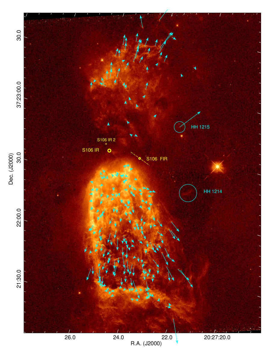
Figure 4: Proper motions of selected compact features superimposed on the 2011 [Nii] image in the S106 reference frame, measured using the cross-correlation methods described in the text. The vector lengths correspond to the motions over the next 400 years. The positions of S106 IR, S106 IR 2 [the small secondary core found by Beuther et al. (2018)], and S106 FIR are indicated by yellow circles. The dashed line indicates the orientation of the maser jet from S106 FIR. The isolated, fast moving knot to the upper-right of S106 FIR is HH 1215. This image is rotated by 18^o with respect to north.

Figure 5: (a): A plot of the proper motion amplitude for the vectors shown in Figure 4 in the south lobe of S106 as a function of the projected distance from S106 IR. The dashed black line shows a projected linear proper motion of 1.3 km s^-1 per arc-second, corresponding to a linear velocity gradient of 246 km s^-1/pc. The red dots show the motions designated as fast at a given projected distance from S106 IR and so listed in the Tables in the Appendix. The magenta dots represent mostly slower motions and listed as slow in the Appendix. The blue dots correspond to the slow-moving features in the South Bar. (b): A plot of the proper motion amplitude for the vectors shown in Figure 4 in the North lobe of S106 as a function of the projected distance from S106 IR. The color scheme is identical to part (a). The isolated fast knot near the legend is the motion of the compact knot, HH 1215.

4.2 Automated Measurement of Proper motions

Proper motions were measured using a Python code that cross-correlates marked regions in a pair of images. Because the 1995 and 2011 images were taken with different cameras on-board HST that have different image scales and orientations of its pixels, the analysis was conducted on aligned and re-interpolated sub-frames extracted from the registered images. Four pairs of sub-frames shown in Figure 2 were extracted from the full-field 1995 and 2011 mosaiced images shifted into the S106 reference frame using SAOImage ds9. The images were displayed in ds9 with the 2011 epoch image displayed at full resolution using the ds9 align function to so that the x- and y-pixels are aligned east-west and north-south, respectively. Matching the 1995 epoch image to the 2011 image using the WCS resulted in a magnification of the drizzled 1995 epoch image by a factor of 1.14944. This sub-frame was interpolated onto a pixel grid identical to the aligned 2011 epoch image. For each of the four sub-fields, the resulting image pairs were saved as fits files to be used as input for proper motion measurements. In a final step, the intensity scales on each image pair were normalized to have similar peak intensities.

The Jupyter Notebook CrossCorrelate.ipynb uses the Python 3.0 package SciPy.signal and the image$\_$registration package from https://pypi.org/project/agpy/. CrossCorrelate.ipynb ingests the sub-field image pairs along with a user-provided ds9 Region file containing the pixel coordinates (Points) of emission peaks on one of the sub-frames. Because the 2011 epoch image has better signal to noise and smaller original pixel scale, it was designated the reference image. The user specifies the number of pixels along each side of a measurement box centered on the features marked by Points. CrossCorrelate.ipynb finds the actual intensity maximum in each measurement box on the reference image (the 2011 image) and re-centers the box on this peak. Measurement box-sizes used in the analysis range from 20 by 20 pixels for compact features to over 200 by 200 pixels for large features. For each marked point, the data inside the measurement box on the 1995 and 2011 images are cross-correlated. The offset of the peak of the resulting cross-correlation image from the center of the box is used as an estimator of the proper motion. When the more recent 2011 epoch images is used as the reference image, the sign of the motion is reversed to give the proper motion.

The output of CrossCorrelate.ipynb consists of an SAO Image DS9 region file containing the measured displacement vectors along with the measurement boxes and a formatted (LaTeX) table of positions and proper motions. The region file shows the measurement boxes and the proper motion vectors scaled to represent motions over the next 400 years. Figure 4 shows the results on the 2011 epoch image. Tables in the Appendix (8 to 10) list the peak positions of features, the proper motions in mas yr^-1, the speed in km s^-1, and the direction (position angle) of the motion in each of the four sub-fields. Each entry in the Tables is given a sequential identification number ranging from 1 to 194 for the southern lobe and from 1 to 51 for the northern lobe. The numbers start in the southwest corner of sub-fields S2 and N1 and increase towards the east and north. These numbers are also indicated in the four figures in the Appendix, Figures 12 to 15.

CrossCorrelate.ipynb can be used to automatically identify all intensity maxima above a chosen intensity value and minimum separation criterion. However, this approach resulted in a large number of ‘faulty’ proper motions shown to be incorrect by visual inspection. The likely causes for the misbehavior of the code are discussed below. For the analysis presented here, we marked 245 locations on the 2011 image for analysis which are deemed to be representative of the overall motions in each portion of S106 by visual inspection. As can be seen by from the movies shown in the electronic version of this paper (or by blinking the provided fits files), these selected points are a good representation of the overall proper motion vector field.

Measurements made with CrossCorrelate.ipynb are subject to several limitations and types of error. The code works best for bright, compact, and isolated knots or stars. But, most of the emission in S106 originates from extended structure, crowded clusters of clumps, forward and backward facing bow-shapes, and filaments. Features with low signal-to-noise ratios have larger uncertainties (in general, the 1995 image has a lower signal-to-noise ratio than the 2011). The fastest feature (#1 in Table 8 is the tip of a bow-shaped feature in the lower-right corner of the S2 field. It has a proper motion of $\sim$167 km s^-1, making it the second fastest object in S106 (the Herbig-Haro object HH 1215 - entry 1 in Table 10 in the S1 field is faster). But the object is very dim on the 1995 image. Visual inspection shows that its motion is likely to have an uncertainty of tens of km s^-1.

In elongated structures such as filaments with relatively constant intensity, only the component of the motion parallel to minor dimension (orthogonal to the filament) can be trusted. The derived position-angle of the proper motion vector can be very uncertain. For extended or complex, clumpy structure, the entry of a bright clump into the measurement box on the 2011 image (or the exit of a clump) which was not in the measurement box on the 1995 image can result in a nonsensical proper motion vector. The entry and exit of dimmer features into the 2-nd epoch image was found to bias the cross-correlation results towards lower speeds. The selection of peaks and the measurement box size was based on our desire to avoid the entry of new features and the departure of others on the 2011 image in the measurement box. Measurement box sizes of 41 by 41 pixels (on the 2011) image were used for the results presented here. In summary, the results of automatic measurements require confirmation by visual inspection.

4.3 Results: Supersonic Nebular Expansion

The velocity on the plane of the sky is given by $V=4.7405~{}PM_{\rm mas/yr}~{}D_{\rm kpc}$ km s^-1 where $PM_{\rm mas/yr}$ is in mas yr^-1 and $D_{\rm kpc}$ is in units of 1 kpc. Thus at 1.09 kpc, $V=5.167~{}PM_{mas/yr}$ (km s^-1). The approximately 15-year interval between the two epochs reveals that most of the narrow-band emission in the nebular interior traced by H$\alpha$ and [Nii] is expanding away from S106 IR with a mean proper motion of $\sim$14 mas yr^-1 or $\sim$70 km s^-1 at the 1.09 kpc distance of S106, $\sim$7 times the sound speed in photo-ionized plasma and 5 times the typical expansion speed in Hii regions (O’Dell, Ferland & Peimbert, 2017; O’Dell, 2018).

Figure 4 shows proper motion vectors of selected regions superimposed on the 2011 epoch image. In the southern lobe of S106, compact nebular features move towards the south and southwest (PA$\sim$190^o to $\sim$220^o). In the northern lobe of S106, compact nebular features move towards the north and northwest (PA$\sim$330^o to $\sim$360^o). In the northern lobe, only a few proper motions could be measured within $\sim 30$″ of S106 IR because of the high extinction towards this region. The proper motions are closely aligned with the orientations of the nebular lobes with motions generally pointing away from S106 IR. Figure 4 shows that the fastest motions are far from S106 IR and that the motions show a systematic deflection towards the west (e.g. exhibit C-shaped symmetry with respect to S106 IR). As discussed below, the two nebular lobes together also exhibit a C-shaped bend towards the west.

Figure 5 shows the amplitudes of all vectors plotted in Figure 4 as a function of the projected distance from S106 IR. Several general trends are apparent. The proper motions fill-in a region between zero speed and a line indicating a linear increase in speed with increasing projected distance from S106 IR. The dashed line in Figure 5 indicates a velocity gradient of 246 ${\rm km~{}s^{-1}~{}pc^{-1}}$. Thus, the upper bound on the speeds increases with increasing distance from S106 IR. While within $\sim$30″  of S106 IR, motions are typically slower than $\sim$40 km s^-1, motions at larger projected distance are faster. The fastest motions are southwest and northwest of S106 IR. Here, some features have proper motions up to about 30 mas yr^-1, corresponding to a speed of $\sim$150 km s^-1.

The fastest motions tend to avoid the bright projected walls of the Hii region. Along the projected eastern edge of the southern lobe and in the South Bar located about 1′ south-southwest of S106 IR, proper motions are either absent or slower than about 30 km s^-1. Because of the high extinction towards the northern lobe, it is not clear if the pattern of slower motions along the lobe walls also holds. There are some features in the lobe interior farther from S106 IR than 30″ that are also moving slowly. Differential motion is evident when the images are blinked in DS9 or viewed as the movies (shown in the electronic version of this paper). These slow-moving features may be close to the foreground or background walls of the nebular lobes along lines of sight through the lobe interior. Consequently, as shown in Figure 5, at any particular projected separation from S106 IR, a range of proper motions are seen from low values to a maximum value which increases with projected separation from S106 IR. Blinking of the images shows filaments and knots just north of the South Bar approaching this quasi-stationary structure. This behavior provides confirmation that, despite the lack of stars near the South Bar, the image registration is good.

Figure 5 shows the amplitudes of fastest nebular motions in the north and south lobe regions tend to avoid the eastern lobe edges and the South Bar. Figure 5 shows that for the motions in the nebular lobe interior and excluding the South Bar, the expansion pattern shows increasing proper motions with increasing projected distance from S106 IR (a ‘Hubble flow’). The proper motions are shown in each of the four sub-regions in greater detail in Appendix A as vectors superimposed on the 2011 sub-frames.

Appendix B shows difference images obtained by matching the mean flux of the nebular emission in the 1995 H$\alpha$ image with the mean flux of the 2011 [Nii] image and taking the difference. In these figures, the 1995 epoch image is shown in black, while the 2011 image is shown in white. In the electronic version of this manuscript, we present MP4 movies showing the changes and motions in the four sub-fields between 1995 and 2011.

We compared the positions and proper motions of field stars measured on our images with the motions measured by Gaia for over two dozen stars in the same field. For the majority of stars, the motions agree to about 2 mas yr^-1, and for motions as large as 6 mas yr^-1 the stellar proper motion directions on our images agree with those measured by Gaia EDR3 to better than $\sim$15^o.

5 Radio and Near-Infrared Images

5.1 A C-Shaped Bend in the Ionized Plasma

Figure 3 shows a previously unpublished, low-resolution but deep $\sim$4.8 GHz (6 cm) radio continuum contour map of S106 superimposed on the image shown in Figure 1. The radio contours show that the northern lobe has similar intensity and size to the southern lobe. However, the northern lobe is deflected towards the west by about 45^o with respect to the axis of symmetry of the southern lobe and the axis of the cavity seen in the far-infrared images shown in Appendix C.

The bright bar located 1.2′ south of S106 IR (South Bar) is a prominent radio continuum emission feature. There is a second bright bar at the northwest end of the northern lobe, also about 1.2′ from S106 IR. This ‘Northwest Bar’ is dimmer at 4.8 GHz than the South Bar by about a factor of two. This feature is not seen in visual wavelength images due to foreground extinction but apparent in the Br-$\gamma$ image discussed below. Motivated by the radio images, we obtained deep near-IR images of S106 in the 2.16 $\mu$m Br-$\gamma$ hydrogen-recombination line which is much less impacted by extinction than H$\alpha$.

Figure 6 shows a continuum-subtracted Br-$\gamma$ image of S106 with 0.9″ angular resolution. This image shows the C-symmetric bend and both the South and Northwest Bars at the ends of the southern and northern lobes of S106. The locations of S106 IR, S106 FIR, and the 0.2 M_⊙ secondary core (scaled to a distance of 1.09 kpc) found 4″ northwest of S106 IR by Beuther et al. (2018) are marked. The orientation of the protostellar outflow from S106 FIR traced by H₂O masers (Furuya et al., 1999, 2000) is indicated by a red line.

5.2 Cavities Surrounding S106 IR and the S106 Ionized Nebula

In the high-resolution radio images of Bally, Snell & Predmore (1983), there is a roughy 8″ by 11″ elliptical cavity flanked by bright free-free emission centered about 4″ west of S106 IR. This feature is also clearly seen in the Br-$\gamma$ images. The major axis of this structure is at PA$\sim$15^o. The southern and western parts of this elliptical feature are also seen in the HST images where the brightest H$\alpha$, [Nii], Br-$\gamma$, and radio continuum emission is located. This inner cavity is bounded by the brightest [Cii] and Oi emission in S106 (Simon et al., 2012; Schneider, et al., 2018). The cavity walls have very low proper motions. The relatively low free-free, Br-$\gamma$, and H$\alpha$ emission in the cavity interior compared to the S106 nebular lobes suggests that the cavity has low density. It may have been evacuated by the slow stellar wind powered by S106 IR.

On larger scales of several arcminutes, the S106 Hii region is located in the interior of a roughly cylindrical cavity with limb-brightened walls at mid- to far-IR wavelengths. The cavity walls are seen clearly in mid to far-IR images (Adams et al., 2015) and in molecules (Schneider et al., 2002). In Spitzer 3.6 to 8 $\mu$m images, the bright part of the cavity containing the Hii region is surrounded by straight and nearly parallel walls, is about $\sim$ 90″ ($\sim$ 0.48 pc) wide and $\sim$400″ (2.1 pc) long, with its axis of symmetry oriented towards PA$\sim$ 15^o to 20^o (see Appendix C). S106 IR is displaced from the axis of symmetry toward the east by about 25″ (0.13 pc). The Spitzer/IRAC 3.6 and 4.5 $\mu$m images show a concentration of stars in S106 with the centroid of the distribution centered within the cylindrical cavity and 15 to 30″ west of S106 IR. It is possible that this cylindrical cavity is the fossil remnant of a bipolar outflow powered by S106 IR produced during its main accretion phase as it grew from a sub-stellar mass object to its current mass. Various color combinations of the mid- to far-IR data are presented in Appendix C.

Figure 6: The continuum subtracted Br-$\gamma$ image shown with an inverted logarithmic grey scale. The South Bar and Northwest Bar are indicated. The thick red circle in the middle of the figure marks the location of S106 IR. The small red circle at the upper-left edge of the circle marking S106 IR indicated the location of the faint secondary continuum source found by Beuther et al. (2018) northeast of S106 IR. The circle with a line marks the location of S106 FIR; The line indicates the direction of the outflow from S106 FIR (Furuya et al., 1999, 2000). The dashed cyan oval shows the 8″ by 11″ cavity discussed in the text. A version of this image emphasizing the faint emission is shown in the Appendix.

5.3 Molecular Hydrogen Images

Figure 7 presents a continuum-subtracted H₂ image of S106. The H₂ morphology is different from both the radio and hydrogen recombination line emission. The brightest H₂ emission is within $\sim$30″ of S106 IR. To the south, west, and north, the H₂ emission closely follows the Br-$\gamma$ and radio continuum which reveals a limb-brightened cavity with a radius ranging from 8 to 11″. The brightest H₂ emission occurs 1″ to 3″ outside this cavity. Such a separation between the hydrogen ionization front (I-front) and the peak of the H₂ emission is consistent with PDR models. Assuming that the penetration column density (the column density between the I-front and the peak of the fluorescent H₂ emission) of non-ionizing far-ultraviolet (FUV) radiation is $N_{PDR}=2\times 10^{21}$ cm^-2 ($A_{V}\sim$1), the volume density of the gas between the I-front and the H₂ photo-center must be $n(H)\approx N_{PDR}/\Delta x_{PDR}$ = 2 to 6$\times 10^{4}$ cm^-3.

The Hii region is surrounded by a scalloped, inverted C-shaped PDR with a radius of about 1 to 1.5′ wrapping around the Hii region from the south, through the west, and to the north. To the south, the PDR forms a clumpy ridge. To the east and northeast, the PDR consists of filaments pointing away from the nebular core and oval cavity. These features appear to wrap around the dense molecular gas and dust adjacent to the east wall of S106 (Schneider et al., 2002; Schneider, et al., 2018; Simon et al., 2012). They wrap around the prominent finger of dust pointing at S106 IR seen in absorption in the 2 $\mu$m images and emission in dense gas tracers and 350 $\mu$m dust continuum. Schneider, et al. (2018) interpreted this structure as a streamer falling into the core of S106 with an infall rate of $\sim 2.5\times 10^{-4}$ M_⊙ yr^-1.

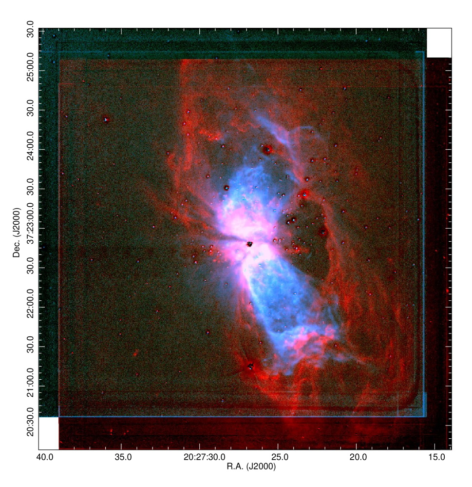
Figure 8: A color composite image showing the continuum subtracted Br-$\gamma$ image (blue and green) combined with the continuum subtracted H₂ image (red). Stars are still visible due to the variable seeing and slight registration errors.

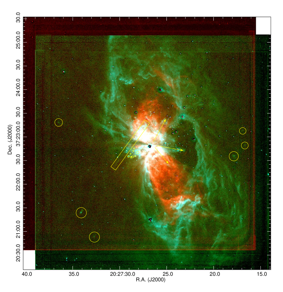
Figure 9: A color composite image showing the continuum subtracted Br-$\gamma$ image (red) combined with the continuum subtracted H₂ image (blue and green). The yellow circles mark compact 2.12 $\mu$m H₂ features that may trace shocks. The three yellow arrows mark H₂ fingers that point away from the vicinity of S106 IR. The yellow box marks the linear feature suspected to trace an H₂jet.

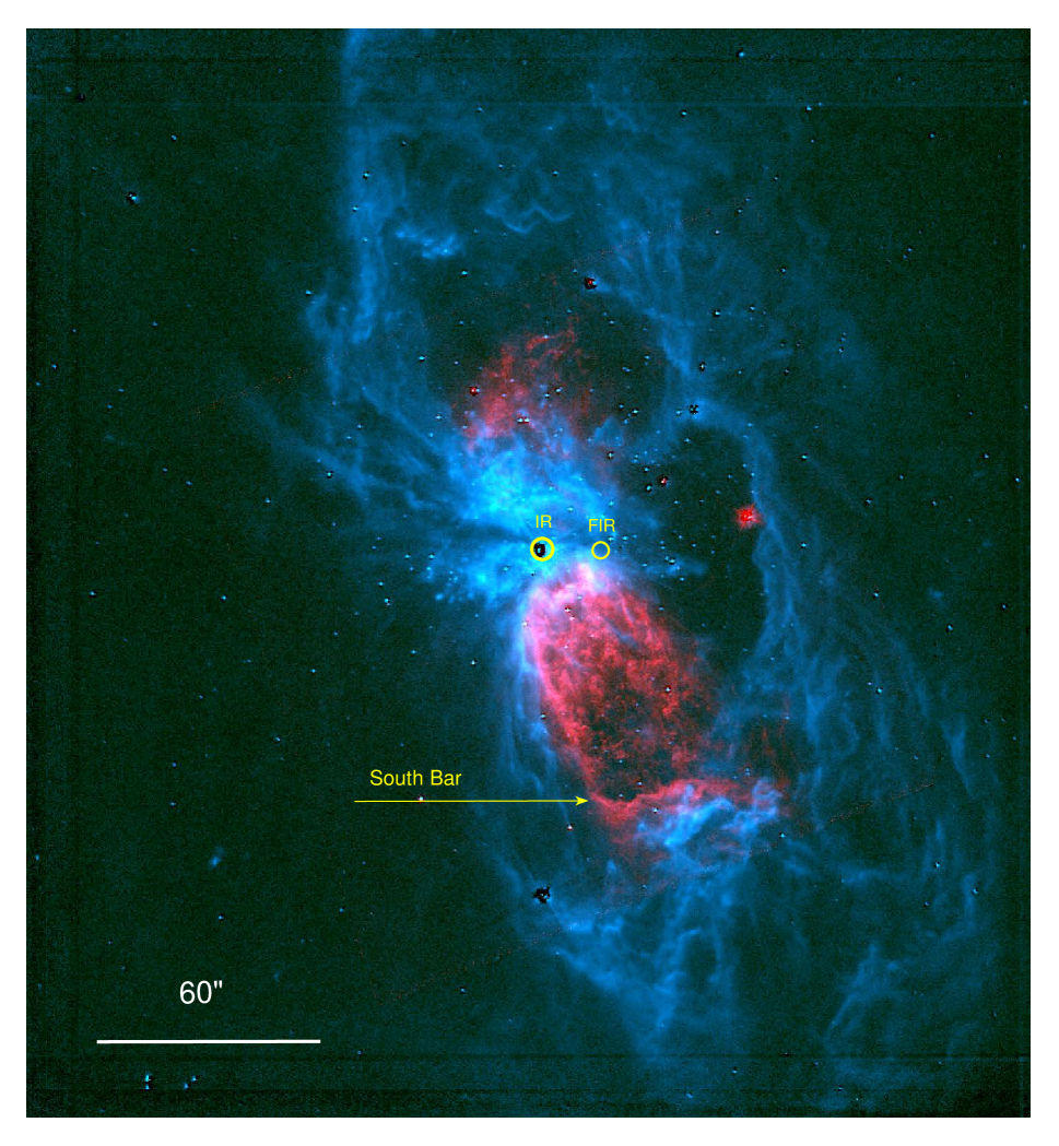
Figure 10: A color image comparing the APO H₂ image (blue), and the HST H$\alpha$ image (red).

Outside the inner 30″ core of S106, the South Bar is the brightest part of the entire PDR structure surrounding S106. The angular separation between the I-front traced by H$\alpha$ and Br-$\gamma$  and the peak H₂ emission ranges from 5″ to 15″, implying nearly an order of magnitude lower density between the I-front and H₂ peaks than in the PDR surrounding the central elliptical cavity. Figures 8, 9, and 10 show color composites made from the continuum subtracted H₂, Br-$\gamma$, and H$\alpha$ images.

The CO maps of Schneider et al. (2002) show the presence of a clump of molecular gas just south of the South Bar. In the H$\alpha$, [Nii], and Br-$\gamma$ images, the South Bar may be the ionized surface of a protrusion of dense gas being overrun by the expanding plasma flow in S106. The small proper motions seen in the ionized gas is consistent with this interpretation. The corrugated and filamentary H₂ emission extending at least 1′ father south indicates that non-hydrogen ionizing FUV radiation penetrates farther into the large, cylindrical cavity seen in the mid- to far-IR and in molecules, presumably either in front, or behind the clump creating the South Bar.

5.4 Candidate Molecular Hydrogen Objects (MHOs)

There are several compact H₂ emission knots beyond the PDR surrounding the Hii region. These are listed as entries 1 through 6 in Table 3 and given the formal designations MHO 4079 through MHO 4084. MHOs 4079, 4080, and 4081 are located west of S106 IR, beyond the western PDR traced by the H₂ and Br-$\gamma$ images. MHOs 4082, 4083, and 4084 are located east of the eastern PDR. These Molecular Hydrogen Objects (MHOs) likely trace shocks in protostellar outflows from YSOs in the S106 cluster, or possibly from S106 IR or S106 FIR. A jet-like feature (entry 7 in Table 3) points to MHO 4083 and is thus given the same designation. MHO 4085 refers to the collection of objects likely to originate from S106 IR and are listed as entries 9 to 12 in Table 3. See Davis et al. (2010) for a description of the MHO catalog. Figure 7 shows the location of these MHOs along with their entry numbers in Table 3.

MHO 4081 is located within 5^o of the axis of the outflow from S106 FIR (Furuya et al., 1999, 2000). A bow-shaped H₂ protrusion or finger points to this knot and is therefore also designated MHO 4081. The eastern portion of this MHO extends for $\sim$ 30″ towards the compact knot in the west which is located 93″ (0.49 pc) from S106 FIR and 107″ (0.57 pc) west of S106 IR. Entry 8 (the main body of MHO 4081) is seen in projection toward the 60″ ‘dark bay’ located due west of S106 IR and S106 FIR. A bow-shaped HH object seen in H$\alpha$ and equally in [Sii], HH 1214 discussed below, is located just beyond and below the west tip of this streamer.

MHO 4084, east of S106 IR, is about 5^o north of the axis defined by S106 FIR and MHO 4081. MHO 4084 is 120″ from S106 IR (0.63 pc) and 135″ (0.71 pc) from S106 FIR. S106 IR is $\sim$8″ south of a line connecting the knot in the western part of MHO 4081 and MHO 4084.

Entry 7, labeled MHO 4083 in Table 3 and Figure 7, is a linear feature resembling a jet. It points within one degree of the compact, bow-shaped knot (entry 5) and is thus given the same designation, MHO 4083. At very low levels, there is faint H₂ emission connecting the jet-like feature to knot 5 in Figure 7 (see the deep-cut figure in the Appendix). Thus, this knot which is elongated in the direction of the jet-like-feature may be a terminal bow shock in a highly collimated, jet-like outflow.

A number of fingers of H₂ emission within about 40″ of S106 IR point directly away from this source and therefore are collectively given the designation MHO 4085, centered at 20:27:26.8, +37:22:48 (MHO 4081 is excluded from this because of its possible association with S106 FIR). The arrows in Figures 7 and 9 show the locations and orientations of several bow-shock-like H₂ streamers originating from the vicinity of S106 IR. Entries 9 and 10 in Figure 7 mark bow-shaped streamers whose axes of symmetry point directly away from S106 IR. Several other, unmarked linear features between entries 9 and 10 also point away from S106 IR. Entry 11 marks one of the brightest H₂ knots in S106. This object lies well outside the ionized zone in S106 but in the interior of the PDR. A line connecting S106 IR to entry 11 contains entry 12, located at the eastern tip of a collection of compact H₂ knots which together outline a bow-shaped structure pointing away from S106 IR. Table 3 lists the coordinates of the features marked in Figure 7.

Table 3: Molecular Hydrogen Objects (MHOs) in and Near S106

#	R.A.	Dec.	Comments
1	20:27:16.7	37:22:49	MHO 4079: Compact knot west of S106 IR
2	20:27:16.9	37:23:07	MHO 4080: Compact knot north of MHO 1
3	20:27:17.9	37:22:36	MHO 4081: Compact knot south of MHO 1
4	20:27:32.7	37:20:53	MHO 4082: Compact knot south-southeast of S106 IR
5	20:27:34.9	37:21:24	MHO 4083: Southeast of S106 IR. Jet (#7) and terminal shock?
6	20:27:36.5	37:23:18	MHO 4084: East of S106 IR. Counterflow from S106 FIR ?
7	20:27:28.9	37:22:50	MHO 4083: Jet-like filament in PDR
8	20:27:26.0	37:22:49	MHO 4081: West-facing bow from S106 FIR?
9	20:27:26.4	37:22:54	MHO 4085: Northwest-facing bow from S106 IR
10	20:27:26.2	37:22:47	MHO 4085: Southwest-facing bow from S106 IR
11	20:27:28.1	37:22:40	MHO 4085: Bright knot, part of southeast-facing bow?
12	20:27:29.1	37:22:35	MHO 4085: Tip of southeast-facing bow?

5.5 The ‘Dark Bay’ west of S106 IR and S106 FIR

The near-IR images reveal a large, roughly 60″ diameter ‘dark bay’ west of S106 IR opening towards the west. The west rim of the region is bounded by the H₂ PDR. To the north and south, the cavity is bounded by the ionized plasma in S106, contributing to its C-shaped symmetry (See Figures 6 to 10). This cavity may be shielded from direct UV illumination by S106 IR by a combination of the nearly edge-on disk around S106 IR, the cloud core harboring S106 FIR located 16″ to the west of S106 IR, and possibly a streamer of gas and dust flowing in from the east that overshoots S106 IR. The cloud core is seen as a compact, bright 350 $\mu$m peak in the maps presented by Simon et al. (2012). The peak emission in the core is located between S106 FIR and S106 IR.

The H₂ emission in the PDR at the west end of the 60″ cavity indicates illumination by FUV radiation. If the cavity is primarily created by the shadow of S106 FIR source, then FUV may propagate either in-front of or behind the shadowed region to produce the PDR on the west side of the cylindrical far-IR cavity. Alternatively, the PDR may be illuminated by FUV radiation produced in the Hii region lobes by recombining hydrogen to produce Lyman-alpha light, and/or FUV from S106 IR scattered by dust.

The deep-cut continuum-subtracted Br-$\gamma$ and H₂ images in the Appendix show that there is faint Br-$\gamma$ emission associated with the PDR traced by H₂. In PDRs, the ionized gas associated with ionization fronts is located between the source of Lyman continuum and the peak H₂ emission. In the South Bar, there is a several arcsecond offset between the peak of the H$\alpha$ and Br-$\gamma$ emission and the peak in H₂ with these hydrogen recombination lines peaking closer to S106 IR than H₂. In contrast, the images in the Appendix show that the Br-$\gamma$ emission associated with PDR $\sim$60″ west of S106 IR is either coincident with, or slightly farther from S106 IR than the H₂  emission. This may indicate that the faint Br-$\gamma$ emission is not an indication of local ionization but a Br-$\gamma$ reflection nebula. Br-$\gamma$ emission from the S106 lobes may be scattered by dust in the PDR.

The dark bay may contain lower density neutral gas than the CO cloud east and west of the S106 far-IR cavity. The density has to be sufficiently high to exclude indirect ionization by recombination-generated Lyman continuum shining on this region from the bipolar lobes of S106. Yet, the density has to be low enough to allow non-ionizing FUV photons to produce the PDR. Such gas may emit in the 157 $\mu$m [Cii] line. Simon et al. (2012) presented evidence for such emission.

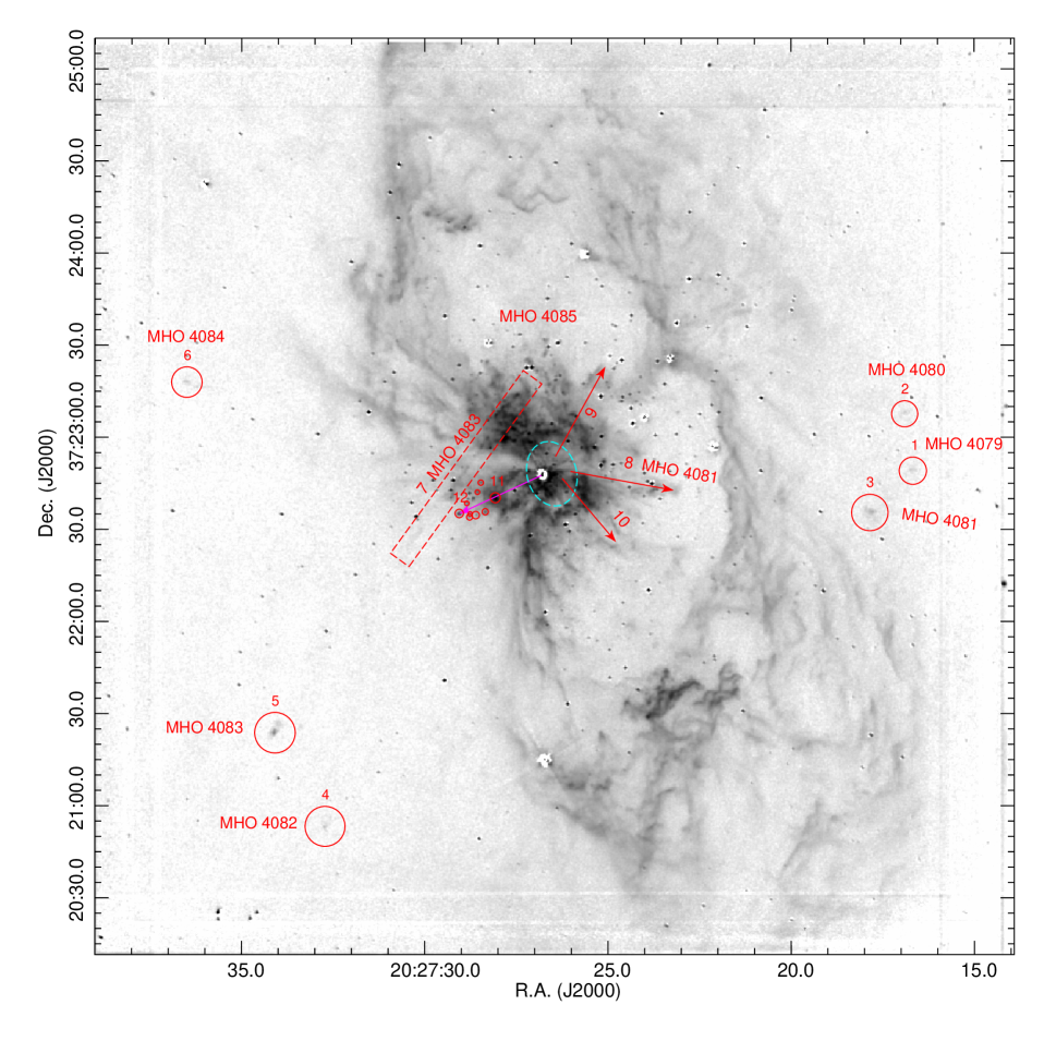
Figure 7: A continuum-subtracted near-infrared image showing S106 the 2.12 $\mu$m H₂ emission line. Large red circles mark H₂ knots located outside the main PDR. Objects labeled 1 through 6 are molecular hydrogen objects (MHOs), likely shocks powered by protostellar outflows. Objects #7 through #12 are seen towards the projected interior of the PDR surrounding S106. The dashed rectangular box shows a jet-like feature which is aimed at object #5 in the lower left of the figure. This is MHO 4083. MHOs 4081 (#3) and MHO 4084 (#6) are located close to the axis of the H₂O outflow from S106 FIR. The three red arrows mark H₂ fingers that point away from the vicinity of S106 IR. The dashed cyan oval shows the 8″ by 11″ cavity discussed in the text and shown in Figure 6. The small, unnumbered circles mark a candidate bow-shock whose axis point back to S106 IR (magenta arrow). The brightest knot, #11, is located in the interior of this bow-shaped feature pointing away from S106 IR. The tip of this structure is object #12. The H₂ features pointing radially away from S106 IR are collectively designated MHO 4085 (except for MHO 4081 which may be associated with S106 FIR). A version of this image emphasizing the faint emission is shown in the Apppendix.

5.6 Is S106 IR Moving with Respect to the S106 Cluster?

The Gaia EDR3 proper motion of S106 IR is $\mu_{\alpha}cos(\delta)$ = -2.183$\pm$0.13 mas yr^-1 and $\mu_{\delta}$ = -5.861$\pm$0.15 mas yr^-1, implying a motion of 6.25 mas yr^-1 towards PA = 200^o in coordinates referenced to the Solar system barycenter. However, it is unclear how reliable the Gaia proper motion measurement is given the extended nebulosity surrounding this star. S106 IR has phot-g mean magnitude’ is 17.87 and the formal proper motion errors may be an underestimate.

On the registered HST images in the S106 reference frame described above, S106 IR moved 0.067″ in the 15.6-year interval between the first and second epoch images. This implies a proper motion of 4.3 mas yr^-1 or $\sim$21 km s^-1 towards position angle of PA = 60°. At this speed the star would have moved about 30″, roughly the distance to the axis or center of the infrared cavity surrounding S106, in about 7,400 years. It would take about 4,000 years to cover the current 16″ distance from the embedded class-0 source S106 FIR located due west of S106 IR. Such a motion might explain the C-shaped symmetry seen in both the nebular plasma and in the nebular proper motions. However, the error on the proper motion of S106 IR is $\sim$2 mas yr^-1. Therefore, it is unclear if the apparent proper motion of S106 IR is real or an artifact of errors in the image de-distortion combined with uncertainties in determining the S106 reference frame. New observations of the position of S106 IR using near-IR, visual, or radio wavelength are needed. New radio observations with the JVLA could be compared to the 1980s data taken with VLA and Merlin. New HST or JWST observations could be compared to the 1995 and 2011 epoch images.

5.7 Candidate Herbig-Haro (HH)

We detected several candidate Herbig-Haro (HH) objects, shock-excited nebulae powered by outflows from forming and young stars, located outside the photo-ionized body of S106. HH 1214 is an arc of emission located about 45″ west of S106 IR at $\alpha$=20:27:22.96, $\delta$=+37:22:39.0 that resembles a bow shock. This 5″-wide feature lies within a few degrees of the orientation of the water maser micro-jet and compact CO outflow emerging from the Class 0 source S106 FIR (Furuya et al., 1999, 2000). Its bow-shape is consistent with being powered by this YSO. This feature is also seen in the Br-$\gamma$ image shown in Figure 6. The candidate bow shock is $\sim$31″ from S106 FIR. The proper motion is difficult to measure because of its diffuse morphology. Proper motions are less than $\sim$20 km s^-1.

A candidate HH object, HH 1215 (# 1 in Table 8 and Figure 11), is located northwest of S106 IR at $\alpha$=20:27:24.20, $\delta$=+37:23:10.5. This object consists of a small group of unresolved knots in a 0.5″ diameter region which exhibits a proper motion of $\sim$176 km s^-1 towards PA = -36° (northwest), making this knot the highest proper motion object in S106. It is shown in Figure 4. However, its not clear if it is related to S106 IR. These HH objects are dimly visible in the F110W and F160W filter images, which may indicate the presence of shock-excited [Fe ii] emission.

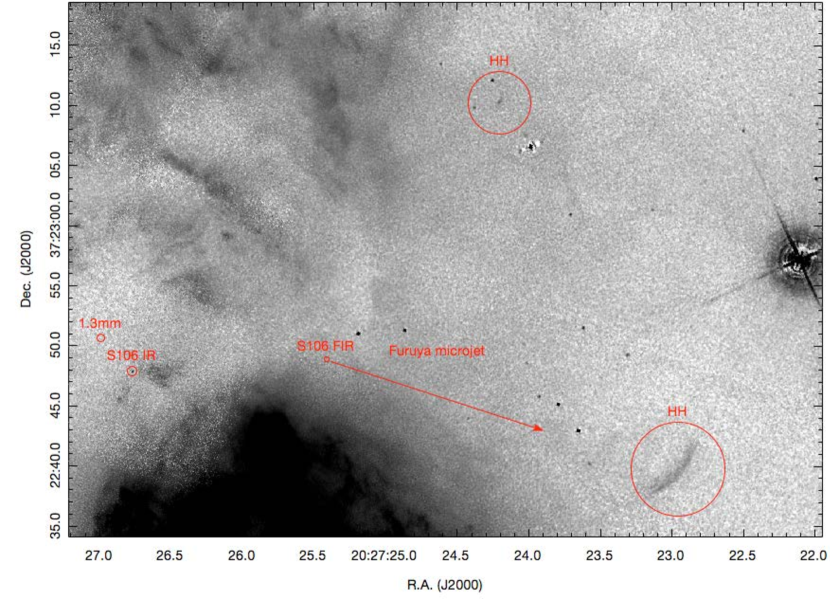
Figure 11: A portion of the 2011 epoch HST [Nii] image showing the candidate HH objects, HH 1214 (lower-right) and HH 1215 (top-center), the locations of S106 IR, the 1.3 mm source found by Beuther et al. (2018), and S106 FIR. The orientation of the H₂O maser and CO micro-jet is indicated (Furuya et al., 2000).

6 Discussion and Interpretation

6.1 The Nature of the Supersonic Motions

Hii regions are expected to expand with a velocity comparable to the sound speed in photo-ionized plasma. At near-solar metallicity, forbidden transitions from trace metals and metal ions with $\sim$2 eV transitions such as the [Oi], [Oii], [Sii], [Nii] and [Oiii] in the near-UV and visual bands, tend to set the temperature of the plasma to around 6,000 to 10,000 K. The resulting sound speed is $C_{s}=(kT/\mu m_{H})^{1/2}\approx$ 10 km s^-1. Density and pressure gradients can increase the expansion velocity by up to a factor of two. Doppler shifts of expanding Hii regions confirm that typical blister Hii regions such as the Orion Nebula exhibit motions of around 5 to 20 km s^-1 away from their parent molecular clouds with faster motions occurring in a few percent of the emitting plasma (O’Dell, 2001; Pabst et al., 2019, 2020). Thus, the highly supersonic expansion shown in Figure 4 is remarkable.

Explosions are not the only mechanism that can produce ‘Hubble flows’. Mac Low et al. (1994) argued that the motions of the W49N 22 GHz water masers were produced by shocked molecular gas accelerated by an an expanding cocoon at the head of a high-speed protostallar jet. McCaughrean & Mac Low (1997) used numerical modeling to argue that the Orion fingers may have been produced by a fast wind interacting with a previously launched slower wind.

We explore several possible explanations for the supersonic expansion of S106:

(1) The fast motion could be an artifact. Large residual errors in de-distortion and registration may remain despite our best efforts to correct them. However, the stellar positions on the images match their expected locations on the de-distorted images to about 0.02″. Nevertheless, the lack of stars in the extreme southwest corner of S106 may make measurements much less reliable. The small proper motions in the South Bar gives us confidence in the registration of the images. New HST images would provide confirmation of the de-distortion and registration accuracy and result in a more precise characterization of the proper motion field.

(2) There could be a systematic offset between the H$\alpha$ and [Nii]. To explain the observed proper motions, such a model must predict a systematic variation of the gap size between the H$\alpha$ and [Nii] emission with the intensity of the emission and distance from S106 IR. As discussed above, the ionization potentials of Hi  and Ni  are similar, with Ni being higher by a fraction of an eV. Thus, in the absence of any true motion, the [Nii] emission, would be expected to peak closer to the ionizing source than the H$\alpha$ emission, not farther away. Because the [Nii] image was acquired after the H$\alpha$ image, any offset between Nii and H$\alpha$ would result in an underestimate of the proper motions.

(3) In the presence of a steeply decreasing density or pressure gradient, the leading edge of a freely expanding plasma cloud undergoing thermal expansion can reach speeds of several times the sound speed in the plasma ($\sim$10 km s^-1). In models of the free-expansion of an isothermal cloud, the mass involved in supersonic expansion decreases exponentially with increasing speed. But, the S106 expansion is seen in most of the emitting plasma, making gradients an unlikely explanation of the proper motions.

(4) Acceleration of gas along the walls of a photo-ionized cavity by stellar wind from S106 IR. The radio, infrared, and visual images of the southern lobe show that there is an evacuated region surrounding S106 IR with a radius of about 11″ (see Figures 1 and 7). The brightest emission is seen from cometary structures lying just outside this region. This bright region may mark the interface between the low-density, wind-dominated zone around S106, and the denser nebular plasma which dominates the emission-line fluxes. However, if the wind reached farther into the nebular lobes, this model predicts that the proper motions should decrease with increasing distance from the source because the ram-pressure of a steady, constant velocity wind decreases as an inverse square law. This is contrary to the observed proper motion field.

(5) Projection effects, combined with the presence of a quasi-spherical, constant velocity, swept-up shell in the foreground driven by a stellar wind can also produce proper motions increasing with projected distance from the wind source. Consider a quasi-spherical shell swept up by the forward shock of a stellar wind from S106 IR. Along the lines of sight close to the source, the shell-expansion velocity vector is aligned close to the line of sight and will exhibit a large blueshift from the foreground portion of the shell (and comparable redshift from the background portion). The proper motion is proportional to the sine of the vector’s angle with respect to the line of sight (or the cosine of the angle of the vector with respect to the plane of the sky). The maximum proper motion will be seen at the projected edge of the shell. This model requires that most of the emitting plasma be located in the shell which surrounds a low-density region. The main problem with this model is that the high radial velocity gas, suspected to trace the zone dominated by a dense wind, is confined to the inner 30″ of S106. Additionally, the nebula morphology is far from that of a quasi-spherical shell. Although the south and Northwest Bars do appear to be limb-brightened, the nebula is better described as consisting of a pair of bipolar, cylindrical cavities.

(6) The bipolar cavities of S106 could represent recently photo-ionized parts of a bipolar molecular outflow launched by S106 IR before it started to emit Lyman continuum radiation. As most stars grow by accretion from their parent molecular cloud cores they power supersonic jets and bipolar winds (Bally, 2016) with speeds ranging from tens to hundreds of km s^-1. As these primary flows interact with the molecular gas in the parent cloud, they produce bipolar molecular outflows that can reach parsec-scale dimensions. The momentum injection rates of such protostellar outflows increases with the source mass and luminosity (Maud et al., 2015a, b). Thus, the most massive stars in a region will generally drive the most powerful and largest outflows. Such a flow likely produced the cylindrical cavity in which S106 is located.

As a massive protostar reaches the main sequence, it starts to ionize its surroundings, which has been pre-processed by the star’s protostellar outflows. Thus, the large nebular proper motions in S106 could have been produced by a previous bipolar molecular outflow phase. In this model, the ionized lobes of S106 trace the recently ionized walls of a fossil bipolar molecular outflow cavity. This model can accommodate a variety of proper motion velocity fields, depending on the history of the mass-loss rate and ejection velocity of S106 IR prior to its reaching the ZAMS, the geometry and opening angle of the flow, and the orientation of the outflow axis with respect to our line-of-sight. The main problems with this model is the very short ($\sim$3,500 year) dynamical age of the S106 nebular lobes. Additionally, this model would predict that there still should be a remnant bipolar molecular flow beyond the Hii region’s ionization fronts in or along the walls of the cylindrical cavity in which the Hii region sits. No such flow had been seen in any species such as carbon monoxide.

(7) S106 may have experienced a ‘Hubble flow’ explosion similar to the Orion fingers emerging from Orion Molecular Core 1 (OMC1) located $\sim$0.1 pc behind the Orion Nebula (Bally et al., 2020, 2017, 2015). In S106, the ejecta are now being photo-ionized by the central OB star, S106 IR. This model predicts that proper motions lie between 0 km s^-1 and a line indicating increasing proper motions with projected distance from the source. Figure 4, shows just such a pattern. The fastest motions are seen at the extreme southwest corner of the southern lobe of S106 and along the northern lobe’s extreme northern edge. The images show the presence of multiple bow-shaped protrusions at the southern end of the S106 Hii region where compact ejecta may be interacting with slower or stationary gas.

The morphology of the plasma in S106 is unique among Hii regions associated with massive young stars. Most Hii regions, such as the Orion Nebula, M16, M17, and others exhibit a relatively smooth plasma morphology. In contrast, as discussed by Bally et a. (1998), the plasma in S106 is highly structured and appears fragmented. It consists of compact knots, along with forwarding and reverse-facing bow-shocks. This morphology is reminiscent of some planetary nebulae, containing hundreds of compact knots and features (an example is the Helix Nebula). The knotty, complex structure of such planetary nebulae is interpreted in terms of the impact of fast winds and outflows on earlier ejected shells of slower-moving but denser ejecta. A combination of Rayleigh-Taylor instabilities, cooling instabilities, and radiation hydrodynamics is thought to be responsible for sculpting these high-contrast structures.

Recent observations of the nearest massive protostars, namely those in Orion OMC1, have shown that a dynamical interaction $\sim$550 years ago ejected two massive and one moderate mass star with speeds of 10 to 55 km s^-1  (Bally et al., 2020). The stellar ejection was accompanied by the launch of an explosive outflow with ‘Hubble flow’ CO streamers whose proper motions and radial velocities increase with projected distance from the ejection center (Zapata et al., 2009; Bally et al., 2017, 2020). These streamers power the shock excited ’fingers’ of molecular-hydrogen emission in this explosive outflow (Bally et al., 2015).

Apparently, S106 exhibits similar behavior. In Orion, the ‘Hubble flow’ pattern with velocities increasing in proportion to projected distance is traced by CO, H₂, and [Fe ii]. In S106, this pattern is revealed by proper motions of the photo-ionized plasma. The fastest proper motions occur in the bow-shaped southwest portion of the S106 southern lobe located about $R\approx$ 96″ from S106 IR. The motions in this part of the nebula reach values of $V\approx$150 km s^-1. This implies a dynamic age for the S106 explosion of order $t_{dyn}=R/V$ $\sim 5\times 10^{3}$ years.

Explosive outflows can be produced by major accretion events such as those that occurred in 2015 in Sh2-255 IRS1, or NGC 6334 I. These events apparently caused the accreting stars to increase their luminosity by $\sim 4\times 10^{4}$ L_⊙ for about 6 months (Caratti o Garatti, et al., 2017; Hunter et al., 2017). Alternatively, as in Orion, the explosion in the gas was associated with the ejection of stars by an N-body interaction. If S106 IR was ejected from its parent core and accretion subsided, its photosphere could rapidly develop main-sequence properties such as the emission of intense Lyman continuum radiation that could start to ionize its surrounding. Having exited the core, its radiation field could ionize its previously ejected bipolar outflow or debris launched during the stellar ejection event.

6.2 Energetics

Radio measurements of the mass of plasma in S106 imply a nebular mass of about 3.1 M_⊙. The mean nebular expansion speed of about 75 km s^-1 implies a nebular kinetic energy, E(Hii)$\approx{\rm 1.7\times 10^{47}}$ erg and a nebular momentum, P(Hii)$\approx$225 M_⊙km s^-1. These rough estimates represent the current kinetic energy and momentum content of the moving nebular plasma. However, when dissipation due to shocks radiating away some of the original kinetic energy is taken into consideration, the energy requirement of the event that set the nebular clumps into motions is larger than $1.7\times 10^{47}$ ergs.

Assuming a Hubble flow explosion with no deceleration, the explosion would have occurred about 3,500 years ago. Assuming the current mass loss rate of S106 IR to be $10^{-6}$ M_⊙year^-1 and a wind velocity of 200 km s^-1, the energy generated in 4,000 years in about ${\rm 1.6\times 10^{45}}$ erg. Thus, the current wind fails by about than two orders of magnitude to explain the nebular energetics.

How much mass must be involved in an accretion event to produce the observed kinetic energy in the S106 Hii region in an energy-conserving interaction of a stationary medium with the ejecta? Given a 15 to 20 M_⊙ star with a radius of R${}_{star}=10^{12}$ cm, the release of $2\times 10^{47}$ ergs of gravitational potential energy requires the accretion of $m>$0.03 to 0.05 M_⊙ onto the star. A short-lived accretion accretion burst delivering this amount of mass onto S106 IR could generate the kinetic energy in the Hii region.

How much mass must be involved in an accretion event to produce the observed momentum in the S106 Hii region ($\sim$225 M_⊙ km s^-1) in an momentum-conserving interaction with ejecta produced by an accretion event? Assuming that a violent accretion event launches ejecta with speed (far from the star) $V_{ejecta}=(GM/R_{star})^{1/2}$ $\sim$500 km s^-1, momentum conservation would require accretion of $\sim$0.5 M_⊙.

6.3 Did S106 IR Have a Bloated Photosphere in the Recent Past?

Massive protostars accreting at high rates tend to develop extended photospheres (Hosokawa & Omukai, 2009). At accretion rates of $\dot{M}>10^{-3}$ M_⊙ yr^-1, accreting massive stars develop AU-scale photospheres because they can not get rid of the entropy developed by their accretion flows. Currently, S106 IR has a mass of order 22 M_⊙ and may still be accreting. At an accretion rate of $\dot{M}>10^{-3}$ M_⊙ yr^-1, S106 IR would only have a mass of 10 M_⊙ 10⁴ years ago. As it grew past 10 M_⊙ it would have developed an AU-scale photosphere which would have been cool, resembling a red supergiant star. The accretion disk feeding the star likely drove a very powerful bipolar jet or wind. Such a bipolar outflow could have produced the axi-symmetric cavities seen at mid- and far-infrared wavelengths.

Models show that as a rapidly accreting, massive protostar grows past $\sim$15 M_⊙, its AU-scale photosphere is expected to shrink and heat, even if high accretion rates persist. As it grew past this mass, S106 IR’s photoshpere would have heated and started to emit Lyman continuum photons. In this scenario, the ionization of the S106 Hii region would have only started within the last few-thousand years. We hypothesize that during its bloated phase, S106 IR either captured its current companion from the S106 cluster, or nearly circularized the orbit of a previously acquired companion. The interaction between a 15 to 20 M_⊙ star with a bloated photosphere could have led to a violent interaction. However, the density and total mass in such bloated stellar envelopes is low and small. The total mass ejected by the common-envelope evolution of a massive star and a $\sim$3 M_⊙ companion over $\sim 10^{4}$ years would likely eject much less less than 1 M_⊙. At least one-half of S106’s plasma is moving supersonically. To deliver the observed momentum in the supersonic motion, debris from an ejected, bloated photosphere the would have to have a much faster speed than the fastest clumps currently seen in S106.

The ejection speed of debris generated by a short-phase of common-envelope interaction is likely to be comparable to the Kepler speed at the mean orbit radius of the companion. At a mean orbit radius of 0.3 AU, a companion orbiting a 20 M_⊙ MYSO the circular mean orbit speed is $\sim$240 km s^-1. Common envelope evolution of a $\sim$20 M_⊙ star with a $\sim$3 M_⊙ companion would have resulted in a substantial increase in the luminosity of the system as the companion moves through the envelope of the primary. We speculate that the resulting radiation pressure could have blown off a portion of a bloated primary’s envelope. Additionally, radiation pressure acting on the surrounding disk and envelope, possibly aided by magnetic fields could have launched additional mass into S106 lobes.

As plausibility argument, we note that the gravitational binding energy of the 3 M_⊙ companion as it orbits the $\sim 20$ M_⊙ primary in a circular orbit with a radius of 0.17 AU is about $E_{B}\sim 4\times 10^{48}$ ergs. If the companion’s orbit shrank to this value from one that is substantially larger, it would have injected much of this energy into the primary’s envelope. If the common-envelope phase lasted $\Delta t$ = 100 years, and injected this much energy into the primary star’s envelope, the resulting increase in the star’s luminosity would be $L\sim E_{B}/\Delta t$ $\sim 3\times 10^{5}$ L_⊙, an order-of-magnitude increase over the current luminosity of S106 IR.

An alternative scenario is that S106 IR was ejected towards the east by a dynamic interaction with a protostar embedded within the cloud core located west of S106 IR where S106 FIR is currently located. Such an interaction may have been similar to the event that occurred in Orion OMC1 about 550 years ago (Bally et al., 2020). S106 FIR is located about 16″ from S106 IR.

Either process could have ejected S106 IR towards the east as suggested by our stellar proper motion measurements. Such an ejection could explain both the proper motions of S106 IR and the C-shaped symmetry of the plasma in S106.

Finally, it is possible that S106 IR is not moving in the reference frame of the S106 cluster. If so, the C-shaped symmetry of the Hii  region would require continued mass inflow towards S106 IR from the east. The orientation of the dust continuum streamers seen at far-infrared and sub-millimeter wavelengths is consistent with the scenario. The C-shaped orientation of the S106 nebular lobes could have been produced by feedback.

6.4 Other Regions Similar to S106

Bipolar Hii regions represent a small subset of Hii regions (Samal et al., 2018). Bipolar structure can result from the formation of a massive star in a sheet of dense gas. As the Hii region forms, ionizes surrounding gas, and blows out of such a sheet, the plasma can be channeled into a bipolar structure. The bipolar geometry, however, may only be seen if the confining sheet is seen nearly edge-on from our vantage point. The expansion rates of such regions will be dominated by thermal pressure of photoionized plasma, and will therefore exhibit expansion with a speed comparable to the sound speed in the plasma, or about $\sim$10 km s^-1, or less. Faster expansion requires additional sources of energy and momentum input such as can be provided by powerful stellar winds or explosive phenomena such as supernovae. As far as we know, S106 is the first bipolar Hii region which exhibits highly supersonic motions.

The morphology and kinematics of S106 are remarkably similar to some proto-planetary nebulae and planetary nebulae such as NGC 6302, OH231.8+4.2, and IRAS 22036+5306. These planetary nebulae exhibit bipolar morphologies, supersonic expansion, and exhibit nebular proper motions increasing with projected distance from the central star. Bipolar planetary nebulae with such Hubble flows may indicate an explosive origin (Soker & Kashi, 2012). The kinetic energies of these nebulae range from $10^{46}$ to $10^{49}$ ergs (Soker & Kashi, 2012; Szyszka et al., 2011). They likely experienced explosions resulting form the merger of a compact binary located at their centers. The total energy released by these explosions is larger than those produced by novae but less than produced by supernovae. They form a class known as ‘Intermediate Luminosity Optical Transients’ (ILOTs). The SPitzer InfraRed Intensive Transients Survey (SPIRITS) has discovered many dozens of infrared transients having a similar luminosity as ILOTs in nearby galaxies (Kasliwal et al., 2017).

7 Conclusions

S106 is the nearest bipolar Hii region ionized by the $\sim$20 M_⊙ primary member of the binary star, S106 IR, which is transitioning from an embedded, protostellar phase onto the main-sequence. The secondary is a $\sim$3 M_⊙ object with a semi-major axis of $\sim$0.17 AU. Archival HST images of S106 obtained in 1995 and 2011 are used to measure nebular proper motions. New near-infrared images of S106 obtained at Apache Point Observatory in the 2.16 $\mu$m Br-$\gamma$ and 2.12 $\mu$m H₂ emission lines are presented.

The main result of this study are:

1) Much of the H$\alpha$ and [Nii] emission in S106 is produced by compact knots whose proper motions are highly supersonic. These motions point away from S106 IR and their speeds increase with projected distance from S106 IR, reaching values larger than $\sim$150 km s^-1  1.5′ ($\sim$0.48 pc) from S106 IR. The proper motion vector field resembles an explosion (a ‘Hubble flow’) . The supersonic motions may have been produced by an explosion about 3,500 years ago, similar to the event that occurred in Orion OMC1 about 550 years ago. The explosion must have released more than $10^{47}$ ergs.

2) Several models for the explosive motions are considered. The explosion may have been produced by a period of common-envelope evolution while the 3 M_⊙ companion was engulfed by the bloated photosphere of S106 IR as it was growing through a mass of 10 to 15 M_⊙ at a high accretion rate. S106 IR may have experienced a dynamical interaction with another star or binary in S106 such as S106 FIR $\sim$3,500 years ago. Finally, S106 IR may have experienced a major accretion burst $\sim$3,500 year ago, accreting $\sim$0.03 to 0.5 M_⊙ or more in an impulsive event. It is unclear which, if any of these mechanisms occurred in S106.

3) The South Bar at the southern end of the Hii region is stationary within the measurement errors. It may trace the ionized surface of a clump of dense gas that is too massive to respond to the outward flow of the Hii region plasma. The HST images show that nebular plasma is blowing past this obstruction on both the east and west sides.

4) At radio wavelengths and in the Br-$\gamma$ emission line, the Hii region exhibits C-shaped symmetry. The northern lobe of the S106 is deflected towards the northwest by about 45^o with respect to the the axis of symmetry of the southern lobe, and the axis of symmetry of the mid- to far-infrared cavity in which the Hii region is embedded. The proper motion vector field also exhibits the same C-shaped symmetry. In the less obscured Br-$\gamma$ hydrogen recombination line, the northern and southern lobes have remarkably similar morphologies. Both lobes have bright bars at their ends, the South Bar and the Northwest Bar.

5) S106 IR and the S106 Hii region lobes are displaced from the center of the cylindrical infrared cavity surrounding the Hii region. S106 IR may have a proper motions towards the east with respect to the parent molecular cloud with a speed of $\sim 20$ km/s. The motion of the star may be responsible for the C-shaped symmetry of the ionized gas in S106. Alternatively, photo-ablation from the dense gas located east of the nebula and possibly falling towards the nebular core, may be responsible for a side-wind which deflects the plasma flow towards the west. Such a side wind may be produced by photo-ablation of dense gas from the cloud along the east-side of S106.

6) There are at least two Herbig-Haro (HH) objects in S106 outside the Hii region. A bow shock is located along the axis of the outflow emerging from the embedded Class 0 protostar, S106 FIR (not to be confused with S106 IR). No proper motions are detected because of its diffuse nature. A second HH object located northwest of S106 FIR exhibits proper motions of 174 km s^-1, the largest proper motion in the S106 field.

7) Near-IR H₂ imaging reveals additional knots suspected to be ‘molecular hydrogen objects (MHOs) - shocks produced in the molecular cloud surrounding S106. These objects are designated MHO 4079 through MHO 4085 in the catalog of Molecular Hydrogen Objects

8) The H₂ images show that the PDR surrounding S106 is asymmetric. The PDR is farther from S106 IR towards the west than towards the east.

9) There is a $\sim$60″ wide, conical cavity located due west of S106 IR between it and the western PDR. The cavity harbors the Class 0 source, S106 FIR at its eastern tip. The cavity may be shadowed by a clump of dust whose emission at 350 $\mu$m peaks between S106 IR and S106 FIR in addition to the edge-on circumstellar matter surrounding S106 IR.

S106 IR joins the growing list of forming massive stars or young massive stars that have spawned explosive outflows. These include the highly obscured OMC1 in Orion (Zapata et al., 2009; Bally et al., 2020), the massive but distant G5.89 star forming region (Zapata et al., 2019, 2020), and DR21 (Zapata et al., 2013). Explosive events from embedded protostars may have a particularly powerful feedback impact on their parent clouds.

Appendix A Proper Motions in the Four Sub-Fields

Figures 12 to 15 show the proper motions in each of the four sub-fields extracted from the final, registered HST mosaics. The figures show the spatial extents of the various proper motion measurement boxes on the 2011 HST image. The associated vector lengths have been scaled to show the motions over the next 400 years. The numbers above each box correspond to the entries in the Tables 8 and Table 10. These Tables list the proper motions in each of the four sub-fields. The vectors shown in red mark the fastest motions at a given projected distance from S106 IR, namely those that lie closest to the dashed lines in the speed vs. projected distance plots. Vectors shown in magenta mostly exhibit lower proper motions. However, in a few cases some of these speeds are as fast as the vectors shown in red. Blue vectors show the very slow motions in the South Bar. Each category (fast, slow, and South Bar) is listed separately in the Tables. The Figures use the same color scheme for these categories of fast and slow vectors. The Northwest Bar is located outside of the field covered by HST. Figure 5 shows plots of the proper motions as a function of projected distance from S106 IR.

Figure 12: Proper motions in the S2 sub-field superimposed on the 2011 [Nii] image in the S106 reference frame, measured using the cross-correlation methods described in the text. The vector lengths correspond to the motions over the next 400 years. Red dots indicate fast motions, magenta dots indicate slower motions, and blue dots indicate slow-moving knots in the South Bar at the South end of the South lobe of S106. The ds9 region files are available as data behind the Figure.

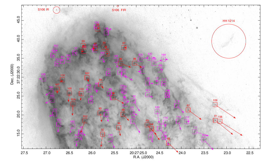
Figure 13: Proper motions in the S1 sub-field superimposed on the 2011 [Nii] image in the S106 reference frame, measured using the cross-correlation methods described in the text. The vector lengths correspond to the motions over the next 400 years. The ds9 region files are available as data behind the Figure.

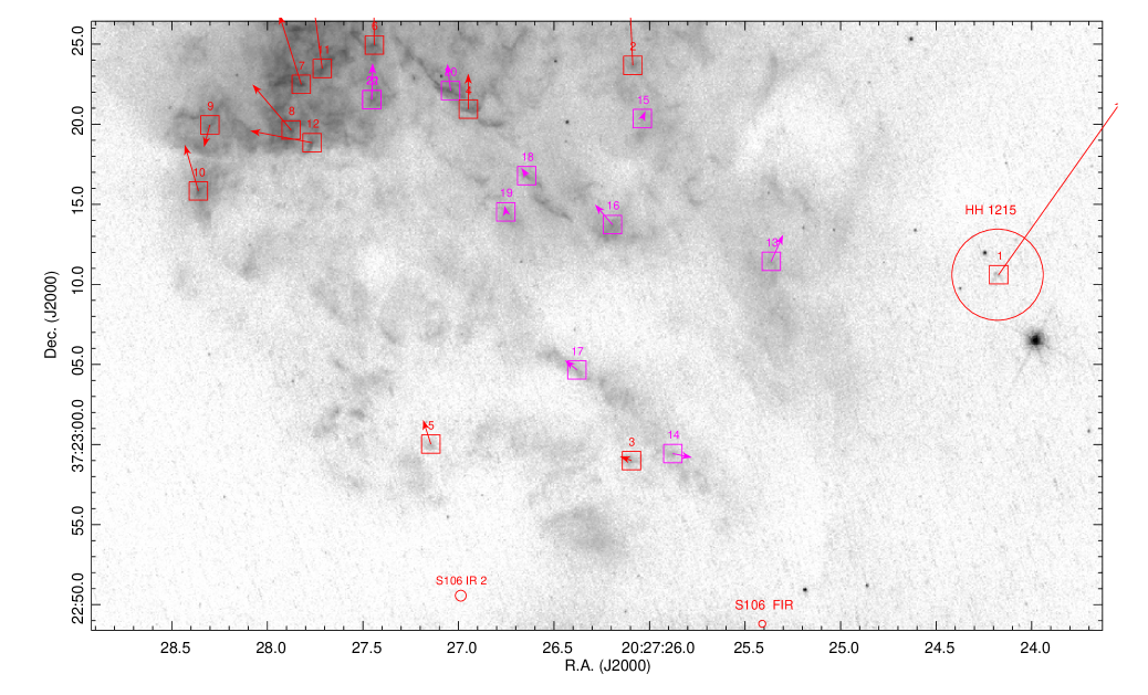
Figure 14: Proper motions in the N1 sub-field superimposed on the 2011 [Nii] image in the S106 reference frame, measured using the cross-correlation methods described in the text. The vector lengths correspond to the motions over the next 400 years. The large arrow on the right marks the proper motion of HH 1215 (entry #1 in Table 9). The ds9 region files are available as data behind the Figure.

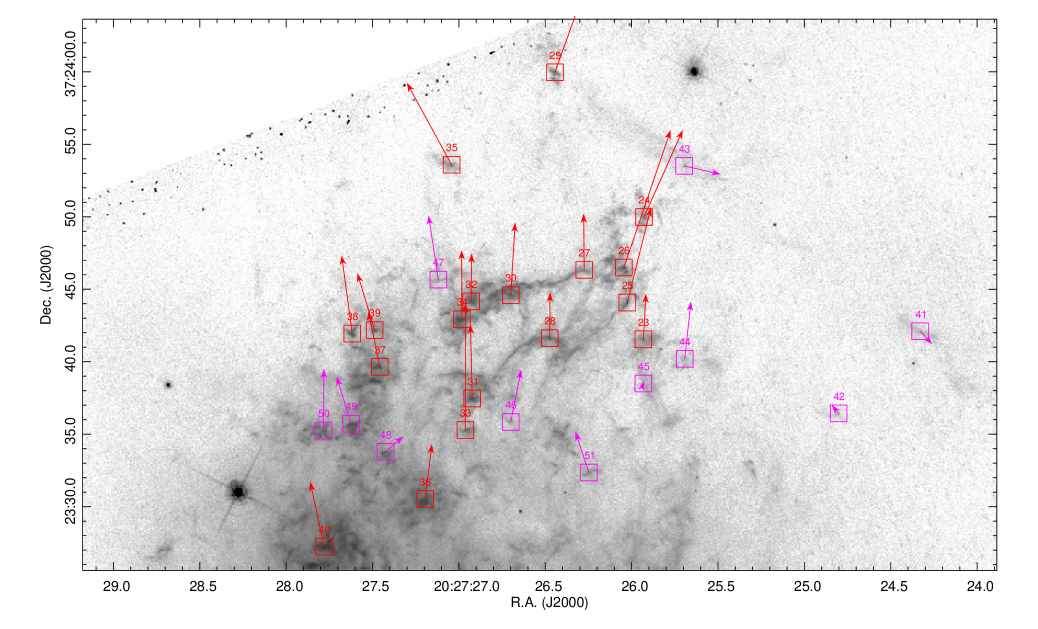
Figure 15: Proper motions in the N2 sub-field superimposed on the 2011 [Nii] image in the S106 reference frame, measured using the cross-correlation methods described in the text. The vector lengths correspond to the motions over the next 400 years. The ds9 region files are available as data behind the Figure.

Table 4: South Lobe Proper Motions Between 1995 and 2011.

#	$\alpha$(J2000)	$\delta$(J2000)	D	PM	V	PA	Comments
	($\arcdeg$)	($\arcdeg$)	(pc)	(mas yr-1)	(km s-1)	($\arcdeg$ )
	South	Lobe	S2	Fast
1	306.8411	37.3598	0.545	32.3	167.1	207
2	306.8426	37.3668	0.438	27.4	141.8	233
3	306.8431	37.3668	0.43	20.5	106.2	243
4	306.8447	37.366	0.416	12.0	62.1	207
5	306.8452	37.3666	0.4	20.7	107.0	226
6	306.8468	37.3683	0.357	17.9	92.5	224
7	306.8478	37.3637	0.404	18.1	93.5	205
8	306.8486	37.3692	0.32	10.6	54.6	232
9	306.8494	37.3692	0.308	12.4	63.8	222
10	306.8502	37.3632	0.384	24.5	126.4	217
11	306.8508	37.365	0.35	10.5	54.2	196
12	306.8524	37.3657	0.322	15.9	82.0	204
13	306.8531	37.3675	0.287	14.0	72.6	195
14	306.8535	37.3664	0.298	18.7	96.7	206
15	306.8539	37.3645	0.328	14.0	72.1	185
16	306.854	37.3644	0.328	11.9	61.5	183
17	306.8538	37.3687	0.26	7.3	37.7	205
18	306.8552	37.3683	0.252	15.5	79.9	195
19	306.8559	37.3693	0.229	10.4	53.8	184
20	306.856	37.3644	0.313	9.8	50.5	176
21	306.8567	37.3635	0.327	15.2	78.5	199
22	306.8567	37.3687	0.233	12.8	66.1	182
23	306.8575	37.3668	0.262	9.0	46.7	188
24	306.858	37.368	0.237	7.6	39.3	176
25	306.8585	37.3691	0.214	8.4	43.4	167
26	306.8586	37.3682	0.229	8.4	43.5	208
27	306.8581	37.363	0.33	15.6	80.5	177
28	306.8601	37.3657	0.273	6.7	34.7	176
	South	Lobe	S2	Slow
29	306.8458	37.3681	0.374	13.0	67.2	251
30	306.8466	37.366	0.389	6.8	35.3	196
31	306.847	37.3646	0.401	6.4	32.8	199
32	306.8471	37.3649	0.395	4.9	25.5	226
33	306.8465	37.3691	0.352	13.0	67.4	224
34	306.848	37.3693	0.328	6.7	34.6	238
35	306.8479	37.367	0.358	12.4	64.1	236
36	306.848	37.3656	0.376	4.8	24.9	202
37	306.848	37.3649	0.384	5.0	25.9	181
38	306.8485	37.3648	0.379	1.5	7.8	162
39	306.8489	37.3652	0.369	13.4	69.1	201
40	306.8493	37.3663	0.349	7.1	36.9	179
41	306.8488	37.3686	0.324	9.4	48.4	243
42	306.8499	37.3692	0.301	7.5	38.6	203
43	306.8498	37.3681	0.318	5.7	29.2	202
44	306.8498	37.3664	0.341	3.5	18.2	198
45	306.8495	37.3658	0.353	12.0	61.9	213

Table 5: South Lobe Proper Motions Between 1995 and 2011 (continued).

#	$\alpha$(J2000)	$\delta$(J2000)	D	PM	V	PA	Comments
	($\arcdeg$)	($\arcdeg$)	(pc)	(mas yr-1)	(km s-1)	($\arcdeg$ )
46	306.8507	37.3635	0.375	10.2	52.5	208
47	306.8517	37.3635	0.364	8.0	41.5	194
48	306.8506	37.3667	0.327	6.1	31.8	206
49	306.8513	37.3664	0.322	2.1	10.7	148
50	306.8515	37.369	0.282	7.0	36.3	247
51	306.8527	37.3688	0.271	5.0	25.6	234
52	306.8527	37.3676	0.29	3.8	19.6	210
53	306.8522	37.368	0.288	2.8	14.2	269
54	306.8513	37.3654	0.338	14.0	72.6	184
55	306.8523	37.3648	0.337	10.6	54.6	186
56	306.8545	37.3653	0.31	11.7	60.4	191
57	306.854	37.3657	0.306	7.5	38.6	199
58	306.8529	37.3663	0.307	1.2	6.4	128
59	306.8539	37.3673	0.282	10.0	51.9	204
60	306.8535	37.3683	0.269	8.7	45.2	206
61	306.8543	37.369	0.25	8.4	43.2	204
62	306.8541	37.3681	0.266	2.5	13.1	204
63	306.8523	37.363	0.367	8.8	45.4	201
64	306.8556	37.3624	0.353	9.5	49.2	194
65	306.8553	37.3637	0.331	6.4	33.0	184
66	306.8579	37.3633	0.324	9.6	49.8	200
67	306.8569	37.3643	0.311	6.2	32.3	177
68	306.8591	37.3653	0.283	3.1	16.3	162
69	306.8583	37.3658	0.276	3.8	19.6	174
70	306.8556	37.3651	0.304	6.4	33.1	187
71	306.8555	37.3657	0.294	8.6	44.5	182
72	306.8558	37.3663	0.281	7.3	37.7	161
73	306.8567	37.3663	0.276	10.4	53.7	182
74	306.8563	37.3678	0.253	6.8	35.3	209
75	306.8567	37.3627	0.341	12.4	64.3	216
76	306.8584	37.3671	0.252	8.8	45.7	181
77	306.8595	37.3682	0.227	4.2	22.0	173
78	306.8601	37.369	0.21	8.8	45.7	164
79	306.8601	37.3657	0.273	6.7	34.7	176
80	306.8602	37.3691	0.208	10.0	51.9	162
	South	Lobe	S1	Fast
81	306.8469	37.3718	0.319	14.9	77.1	230
82	306.8494	37.3726	0.27	10.9	56.6	233
83	306.8512	37.3702	0.271	9.0	46.5	225
84	306.8528	37.3712	0.235	9.2	47.5	215
85	306.8532	37.3715	0.226	9.0	46.5	223
86	306.8543	37.376	0.156	5.7	29.5	238
87	306.8553	37.3772	0.129	2.0	10.2	265
88	306.8554	37.3723	0.187	5.8	30.1	222
89	306.8556	37.376	0.135	7.4	38.2	248
90	306.8563	37.3735	0.158	8.2	42.1	240

Table 6: South Lobe Proper Motions Between 1995 and 2011 (continued).

#	$\alpha$(J2000)	$\delta$(J2000)	D	PM	V	PA	Comments
	($\arcdeg$)	($\arcdeg$)	(pc)	(mas yr-1)	(km s-1)	($\arcdeg$ )
91	306.8558	37.3713	0.198	5.6	28.8	192
92	306.8573	37.3708	0.192	8.5	43.9	173
93	306.8575	37.3724	0.163	6.1	31.8	189
94	306.8575	37.3745	0.13	3.4	17.4	214
95	306.8569	37.3767	0.108	1.0	5.4	-53
96	306.8572	37.3772	0.098	2.3	11.8	-86
97	306.858	37.3771	0.087	1.9	10.0	99
98	306.8577	37.3785	0.077	0.3	1.6	133
99	306.8591	37.3773	0.068	0.6	3.0	45
100	306.859	37.3769	0.075	1.9	10.1	87
101	306.8587	37.375	0.109	3.1	15.8	202
102	306.8589	37.3718	0.163	8.4	43.5	160
103	306.8593	37.3738	0.125	4.6	23.8	174
104	306.86	37.373	0.135	7.8	40.1	177
105	306.8603	37.3738	0.119	6.1	31.7	173
106	306.861	37.3748	0.099	1.9	9.9	148
107	306.8615	37.3741	0.111	3.1	16.0	184
108	306.8464	37.3718	0.326	17.7	91.2	237
109	306.8469	37.373	0.308	16.4	84.6	236
	South	Lobe	S1	Slow
110	306.8479	37.3704	0.316	9.1	47.0	222
111	306.8488	37.371	0.296	9.6	49.8	253
112	306.8495	37.3717	0.276	2.2	11.1	-77
113	306.8504	37.3729	0.25	6.9	35.6	224
114	306.8503	37.3718	0.264	5.9	30.7	194
115	306.8513	37.3737	0.228	1.2	6.2	225
116	306.8513	37.3737	0.228	1.0	5.2	218
117	306.8516	37.3745	0.214	0.8	4.3	63
118	306.8515	37.3717	0.247	3.3	16.9	179
119	306.852	37.3712	0.245	7.3	37.6	216
120	306.8522	37.3725	0.227	7.8	40.4	190
121	306.8523	37.3746	0.203	1.9	9.8	-5
122	306.8531	37.3746	0.189	4.1	21.1	264
123	306.8531	37.3737	0.199	3.9	19.9	241
124	306.8516	37.3706	0.259	6.4	33.1	210
125	306.8529	37.3706	0.242	3.9	20.3	201
126	306.8545	37.3717	0.206	9.0	46.4	211
127	306.8536	37.3754	0.173	3.1	15.9	95
128	306.8538	37.3763	0.162	5.6	29.1	-81
129	306.8525	37.376	0.186	5.9	30.5	-67
130	306.8529	37.3764	0.177	3.7	19.3	-82
131	306.8546	37.3724	0.194	4.4	22.5	240
132	306.8544	37.3733	0.185	8.3	42.8	211
133	306.8553	37.374	0.164	5.2	27.1	189
134	306.8555	37.374	0.16	5.7	29.7	196
135	306.8553	37.3752	0.148	7.2	37.3	236

Table 7: South Lobe Proper Motions Between 1995 and 2011 (continued).

#	$\alpha$(J2000)	$\delta$(J2000)	D	PM	V	PA	Comments
	($\arcdeg$)	($\arcdeg$)	(pc)	(mas yr-1)	(km s-1)	($\arcdeg$ )
136	306.8557	37.3754	0.141	6.0	31.3	231
137	306.8567	37.3753	0.127	0.7	3.7	108
138	306.8561	37.3762	0.125	5.1	26.5	196
139	306.8552	37.373	0.179	3.4	17.7	-48
140	306.8569	37.3723	0.171	5.0	25.9	195
141	306.8567	37.3738	0.149	4.6	23.9	196
142	306.8567	37.3738	0.149	4.8	24.6	194
143	306.8578	37.3742	0.131	3.2	16.3	175
144	306.8566	37.3704	0.204	6.4	33.0	207
145	306.8584	37.3733	0.141	0.7	3.8	158
146	306.8586	37.3741	0.125	2.0	10.5	74
147	306.8593	37.371	0.176	4.1	21.4	231
148	306.8594	37.3707	0.181	3.4	17.4	200
149	306.8597	37.3704	0.185	4.8	24.7	176
150	306.8601	37.3714	0.165	5.0	25.9	158
151	306.8613	37.3715	0.16	5.5	28.4	173
152	306.8617	37.3723	0.146	3.9	20.3	113
153	306.8619	37.3733	0.127	5.0	26.0	114
154	306.8621	37.374	0.115	4.3	22.2	128
155	306.8628	37.3749	0.1	3.0	15.4	89
156	306.857	37.3783	0.093	4.6	23.9	-48
157	306.8598	37.3768	0.068	0.7	3.5	63
158	306.8573	37.3765	0.104	3.9	20.1	201
159	306.8604	37.3763	0.073	1.7	8.7	15
160	306.8616	37.377	0.057	0.4	2.3	65
161	306.861	37.3762	0.073	1.8	9.5	28
162	306.8615	37.376	0.076	0.9	4.9	63
163	306.8619	37.3766	0.064	0.5	2.4	28
164	306.8517	37.3763	0.2	3.1	16.2	263
165	306.852	37.3755	0.2	1.9	10.0	-82
166	306.858	37.377	0.088	2.8	14.5	79
167	306.859	37.3769	0.075	1.9	10.1	87
168	306.8579	37.3787	0.074	0.6	2.8	-32
	S2	South	Bar
169	306.8424	37.3615	0.506	4.5	23.0	50
170	306.8431	37.3612	0.5	6.9	35.8	-89
171	306.8447	37.3619	0.469	1.2	6.2	2
172	306.8462	37.3623	0.445	0.5	2.6	28
173	306.8465	37.3622	0.441	0.8	4.0	28
174	306.8466	37.3616	0.45	4.3	22.0	6
175	306.8469	37.3627	0.43	4.9	25.5	50
176	306.847	37.3618	0.443	0.4	2.1	19
177	306.8475	37.3627	0.423	1.4	7.3	37
178	306.8485	37.3608	0.441	2.1	10.7	103
179	306.8486	37.3624	0.414	0.8	3.9	56
180	306.8491	37.362	0.415	2.2	11.2	143

Table 8: South Lobe Proper Motions Between 1995 and 2011 (continued).

#	$\alpha$(J2000)	$\delta$(J2000)	D	PM	V	PA	Comments
	($\arcdeg$)	($\arcdeg$)	(pc)	(mas yr-1)	(km s-1)	($\arcdeg$ )
181	306.8494	37.3607	0.433	1.7	8.7	67
182	306.8499	37.3622	0.404	4.6	23.8	180
183	306.8502	37.3617	0.409	1.0	5.4	195
184	306.8512	37.3616	0.4	2.2	11.4	166
185	306.8521	37.3617	0.392	1.6	8.1	154
186	306.853	37.3602	0.409	1.7	8.6	143
187	306.8532	37.3609	0.396	2.1	11.0	115
188	306.8536	37.3606	0.399	2.6	13.3	178
189	306.8541	37.3611	0.386	1.4	7.2	0
190	306.8541	37.3607	0.393	3.5	18.0	108
191	306.855	37.3611	0.379	0.6	3.2	152
192	306.8553	37.361	0.38	0.5	2.8	163
193	306.8556	37.3612	0.375	1.8	9.2	173
194	306.8562	37.3615	0.365	0.8	4.2	114

Table 9: North Lobe Proper Motions Between 1995 and 2011.

#	$\alpha$(J2000)	$\delta$(J2000)	D	PM	V	PA	Comments
	($\arcdeg$)	($\arcdeg$)	(pc)	(mas yr-1)	(km s-1)	($\arcdeg$ )
	North	Lobe	N1	Fast
1	306.8507	37.3863	0.238	33.6	173.8	-35	HH 1215
2	306.8587	37.3899	0.197	9.4	48.6	2
3	306.8587	37.3831	0.079	1.9	9.9	70
4	306.8623	37.3892	0.175	5.5	28.5	0
5	306.8631	37.3833	0.071	4.0	20.4	17
6	306.8643	37.3903	0.203	12.7	65.6	0
7	306.8659	37.3896	0.201	11.4	59.0	17
8	306.8661	37.3888	0.189	9.3	48.1	40
9	306.8679	37.3889	0.209	3.5	18.3	165
10	306.8682	37.3877	0.194	7.5	38.6	16
11	306.8655	37.3899	0.203	12.2	62.9	7
12	306.8657	37.3886	0.182	9.8	50.6	79
	North	Lobe	N1	Slow
13	306.8557	37.3865	0.167	4.5	23.4	-24
14	306.8578	37.3832	0.093	3.0	15.7	258
15	306.8585	37.389	0.181	1.3	6.5	-22
16	306.8591	37.3871	0.144	4.1	21.3	41
17	306.8599	37.3846	0.094	2.4	12.3	51
18	306.861	37.388	0.153	1.5	7.6	34
19	306.8615	37.3874	0.141	1.0	5.0	12
20	306.8627	37.3895	0.182	4.2	21.6	6
21	306.8644	37.3893	0.186	5.6	29.1	-1
22	306.8644	37.3893	0.186	5.6	29.1	-1
	North	Lobe	N2	Fast
23	306.858	37.3949	0.291	7.9	40.6	-3
24	306.858	37.3972	0.335	16.4	84.8	-24
25	306.8584	37.3956	0.303	16.9	87.2	-14
26	306.8585	37.3963	0.315	25.0	129.3	-18
27	306.8595	37.3962	0.311	9.6	49.9	0
28	306.8603	37.3949	0.285	7.8	40.5	0
29	306.8602	37.4	0.382	22.1	114.4	-19
30	306.8612	37.3957	0.3	12.5	64.5	-3
31	306.8622	37.3937	0.262	12.7	65.8	1
32	306.8622	37.3956	0.298	8.2	42.6	0
33	306.8623	37.3931	0.251	21.8	112.7	0
34	306.8624	37.3953	0.292	11.9	61.3	0
35	306.8627	37.3982	0.348	16.1	83.1	28
36	306.8633	37.3918	0.228	9.5	49.1	-7
37	306.8644	37.3943	0.279	9.8	50.7	11
38	306.8651	37.395	0.294	13.6	70.1	7
39	306.8645	37.3951	0.293	10.2	52.9	16
40	306.8658	37.3909	0.223	11.4	58.8	12
	North	Lobe	N2	Slow
41	306.8514	37.395	0.345	3.0	15.4	223
42	306.8533	37.3935	0.3	1.8	9.4	40
43	306.8571	37.3982	0.357	6.4	33.3	257
44	306.8571	37.3945	0.289	9.9	51.1	-6
45	306.858	37.394	0.276	0.4	1.9	-17

Table 10: North Lobe Proper Motions Between 1995 and 2011 (continued).

#	$\alpha$(J2000)	$\delta$(J2000)	D	PM	V	PA	Comments
	($\arcdeg$)	($\arcdeg$)	(pc)	(mas yr-1)	(km s-1)	($\arcdeg$ )
46	306.8612	37.3933	0.254	9.2	47.4	-11
47	306.863	37.396	0.307	11.2	57.7	8
48	306.8643	37.3927	0.248	4.1	21.0	-48
49	306.8651	37.3933	0.262	8.5	43.8	17
50	306.8658	37.3931	0.263	10.6	54.8	0
51	306.8594	37.3923	0.239	7.4	38.0	18

Appendix B Difference Images

Images showing the difference between the 2011 and 1995 epoch data were formed from the four sub-fields shown in Figure 2. The images were normalized so that the peak nebular emission has a value of about 1.0. The normalized 1995 image was then subtracted from the normalized 2011 image. The results are shown in Figures 16 to 19. In the electronic version of this manuscript, we present mp4 movies showing the proper motions and intensity changes in the four sub-fields between 1995 and 2011. The final mosaic assembled from the 1995 H$\alpha$ data and the 2011 [Nii] image are made available in FITS format. The registered and re-sampled 1995 and 2011 sub-frames used for proper motion measurements in the four sub-fields, S1, S2, N1, and N2, are made available in FITS format.

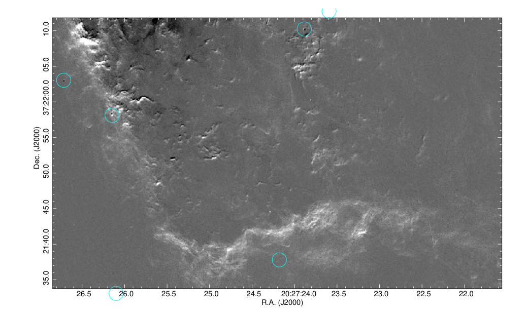
Figure 16: A difference image showing proper motions and changes in the south 2 (S2) field between the 2011 and 1995 epoch HST images in the southern end-cap regions of S106. An animated version of this difference image, blinking between the 1995 and 2011 epochs, is available in the online Journal. The animation is 12 seconds in duration with a cadence of 1 epoch/second; it is not annotated. The FITS files used to construct this difference image are available as the data behind the figure.

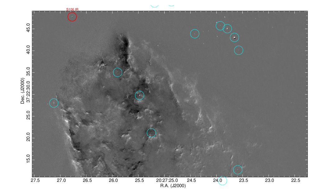
Figure 17: A difference image showing proper motions and changes in the south 1 (S1) fields between the 2011 and 1995 epoch HST images. The time interval between these images is 15.6 years. Cyan circles show the stars used to register this portion of the multi-epoch HST data. The 2011 image is shown in white. The 1995 image is shown in black. This Figure shows the field containing the inner part of the southern lobe of S106. An animated version of this difference image, blinking between the 1995 and 2011 epochs, is available in the online Journal. The animation is 12 seconds in duration with a cadence of 1 epoch/second; it is not annotated. The FITS files used to construct this difference image are available as the data behind the figure.

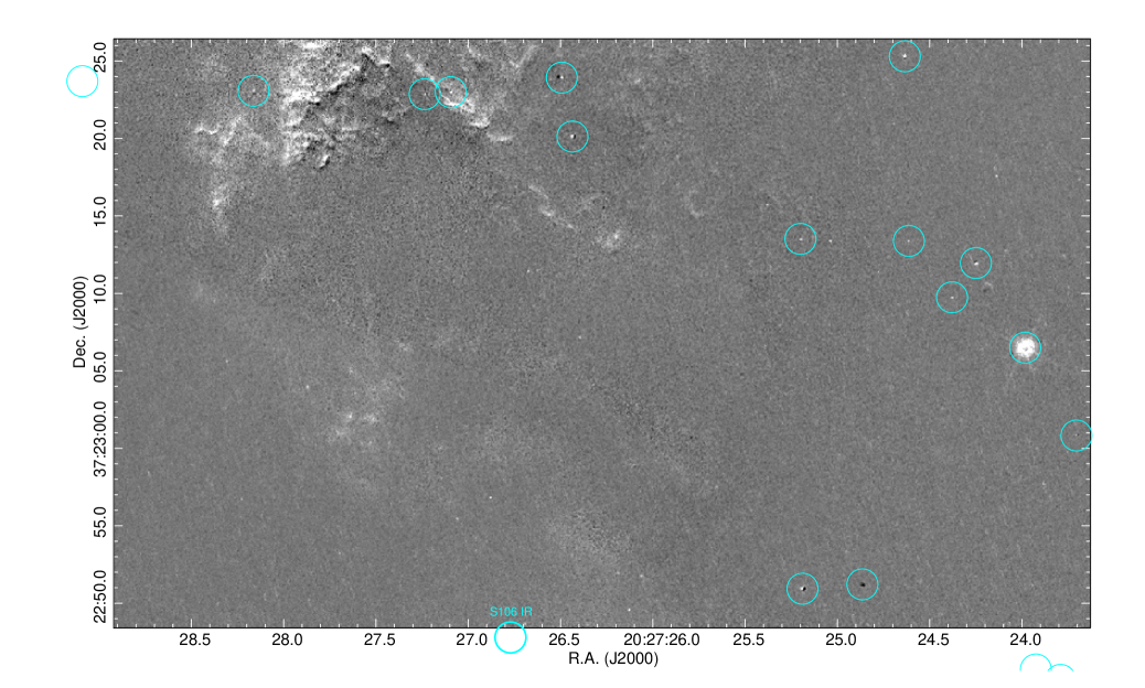
Figure 18: A difference image showing proper motions and changes in the north 1 (N1) field between the 2011 and 1995 epoch HST images in inner part of the northern lobe of S106. An animated version of this difference image, blinking between the 1995 and 2011 epochs, is available in the online Journal. The animation is 12 seconds in duration with a cadence of 1 epoch/second; it is not annotated. The FITS files used to construct this difference image are available as the data behind the figure.

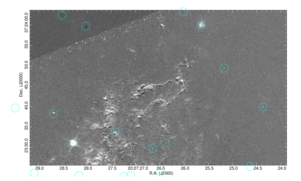
Figure 19: A difference image showing proper motions and changes in the north 2 (21) field between the 2011 and 1995 epoch HST images in the portion of the northern lobe of S106. The interval between images is 15.1 years. An animated version of this difference image, blinking between the 1995 and 2011 epochs, is available in the online Journal. The animation is 12 seconds in duration with a cadence of 1 epoch/second; it is not annotated. The FITS files used to construct this difference image are available as the data behind the figure.

Appendix C Spitzer and Herschel mid-IR Images

Figure 20 shows that the Hii region sits inside a roughly cylindrical, $\sim$6′  (1.9 pc) long cavity bounded by warm dust and PAH emission at 3.6, to 70.0 $\mu$m. This cavity is more than a factor of two longer and wider than the Hii region at visual, near-IR, and radio wavelengths. S106 IR is displaced from the center of this cavity and located near its eastern edge.

Figure 20 shows a color composite image showing 8, 70, and 160 $\mu$m emission. The cavity walls are clearly seen in the shorter wavelengths (blue in Figure 20). Warm dust in the surrounding molecular cloud is traced by the 70 $\mu$m emission. Note the V-shaped filaments fanning away from the center of the Hii region towards the north an northeast. Also note the bright bar located about 1.3′ south of S106 IR. This feature is also seen at radio frequencies and marks the southern end of the Hii region. The dark feature located 30″ to 60″ west of S106 IR remains dark at all wavelengths to 500 $\mu$m. Thus, this feature may be a cavity in the cloud surrounding S106 that is shielded from illumination by S106 IR by the dense molecular clump containing the Class 0 source, S106 FIR (Furuya et al., 1999, 2000).

Figure 20: Left: A wide-field view showing the cavities surrounding the S106 Hii region in the Spitzer/IRAC 3.6 $\mu$m (blue), 4.6 $\mu$m (green), and 8.0 $\mu$m (red) images. The location of S106 IR is indicated by the red dot in the brightest part of the image. Right: A wide-field view showing the cavities surrounding the S106 Hii region in the Spitzer/IRAC 8.0 $\mu$m (blue), Herschel/PACS 70 $\mu$m (green) and 160.0 $\mu$m (red) images.

Appendix D near-IR narrow-band images

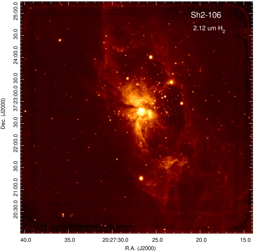
Figure 21: Near-infrared image showing S106 in a narrow-band filter centered on the $\lambda$=2.12 $\mu$m H₂ emission line.

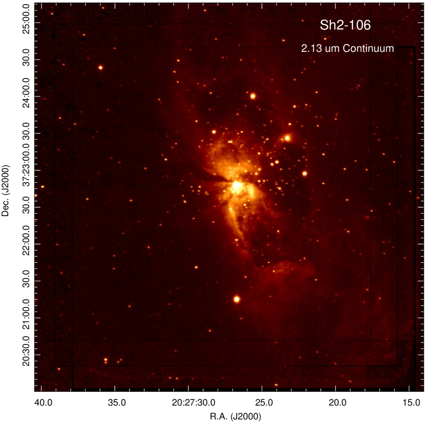
Figure 22: Near-infrared image showing S106 in a narrow-band filter centered at $\lambda$=2.13 $\mu$m off the H₂ emission line.

Figure 21 shows the narrow-band H₂ image taken with the APO 3.5 meter telescope at a wavelength of 2.12 $\mu$m with a filter pass-band of 0.5%. Figure 22 shows the narrow-band H₂- off-line image taken with the APO 3.5 meter telescope at a wavelength of 2.13 $\mu$m with a filter pass-band of 0.5%. These images show some of the members of the S106 cluster.

Figure 23 shows a deep cut of Figure 7 that emphasizes the faint feature of H₂ emission. Figure 24 shows a deep cut of Figure 6 that emphasizes the faint feature of H₂ emission.

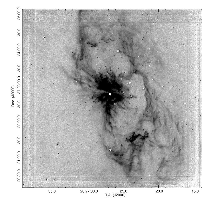
Figure 23: Continuum-subtracted near-infrared image showing S106 in the $\lambda$=2.12 $\mu$m H₂ emission line. The intensity scale on this log display is set to emphasize faint features.

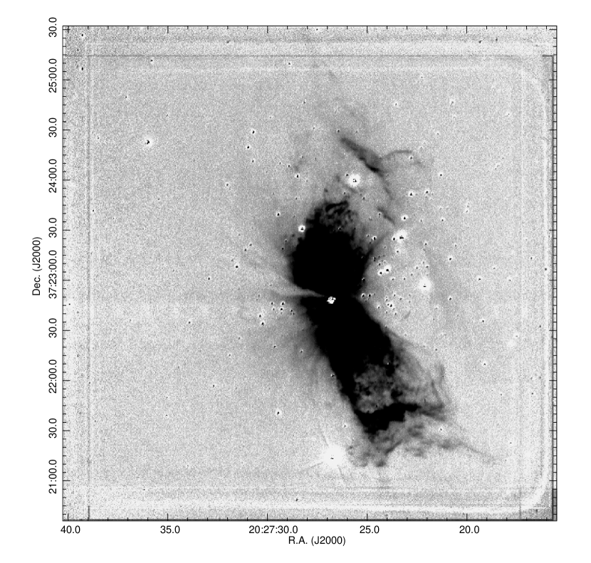
Figure 24: Continuum-subtracted near-infrared image showing S106 in the $\lambda$=2.16 $\mu$m Br-$\gamma$ emission line. The intensity scale on this log display is set to emphasize faint features.

References

- Adams et al. (2015) Adams, J. D., Herter, T. L., Hora, J. L., et al. 2015, ApJ, 814, 54
- Bally & Scoville (1982) Bally J., & Scoville, N. Z. 1982, ApJ, 255, 497
- Bally et a. (1998) Bally J., Yu K. C., Rayner J., Zinnecker H., 1998, AJ, 116, 1868