Variational Auto-Encoder Architectures
that Excel at Causal Inference

Abstract

Estimating causal effects from observational data (at either an individual- or a population- level) is critical for making many types of decisions. One approach to address this task is to learn decomposed representations of the underlying factors of data; this becomes significantly more challenging when there are confounding factors (which influence both the cause and the effect). In this paper, we take a generative approach that builds on the recent advances in Variational Auto-Encoders to simultaneously learn those underlying factors as well as the causal effects. We propose a progressive sequence of models, where each improves over the previous one, culminating in the Hybrid model. Our empirical results demonstrate that the performance of all three proposed models are superior to both state-of-the-art discriminative as well as other generative approaches in the literature.

1 Introduction

As one of the main tasks in studying causality (Peters et al., 2017; Guo et al., 2018), the goal of Causal Inference is to determine how much the value of a certain variable would change (i.e., the effect) had another specified variable (i.e., the cause) changed its value. A prominent example is the counterfactual question (Rubin, 1974; Pearl, 2009) “Would this patient have lived longer (and by how much), had she received an alternative treatment?”. Such questions are often asked in the context of precision medicine, hoping to identify which medical procedure $t\in\mathcal{T}$ will benefit a certain patient $x$ the most, in terms of the treatment outcome $y\in{\cal R}$ (e.g., survival time).

The first challenge with causal inference is the unobservability (Holland, 1986) of the counterfactual outcomes (i.e., outcomes pertaining to the treatments that were not administered). In other words, the true causal effect is never observed and cannot be used to train predictive models, nor can it be used to evaluate a proposed model. The second common challenge is that the training data is often an observational study that exhibits selection bias (Imbens and Rubin, 2015) — i.e., the treatment assignment can depend on the subjects’ attributes. The general problem setup of causal inference and its challenges are described in detail in Appendix A.

Like any other machine learning task, we can employ either of the two general approaches to address the problem of causal inference: (i) discriminative modeling, or (ii) generative modeling, which differ in how the input features $x$ and their target values $y$ are modeled (Ng and Jordan, 2002):

Discriminative methods focus solely on modeling the conditional distribution $\textrm{Pr}(\,y\,|\,x\,)$ with the goal of direct prediction of the target $y$ for each instance $x$. For prediction tasks, discriminative approaches are often more accurate since they use the model parameters more efficiently than generative approaches. Most of the current causal inference approaches are discriminative, including the matching-based methods such as Counterfactual Propagation (Harada and Kashima, 2020), as well as the regression-based methods such as Balancing Neural Network (BNN) (Johansson et al., 2016), CounterFactual Regression Network (CFR-Net) (Shalit et al., 2017) and its extensions (cf., (Yao et al., 2018; Hassanpour and Greiner, 2019)), and Dragon-Net (Shi et al., 2019).

Generative methods, on the other hand, describe the relationship between $x$ and $y$ by their joint probability distribution $\textrm{Pr}(\,x,y\,)$. This, in turn, allows the generative model to answer arbitrary queries, including coping with missing features using the marginal distribution $\textrm{Pr}(\,x\,)$ or [similar to discriminative models] predicting the unknown target values $y$ via $\textrm{Pr}(\,y\,|\,x\,)$. A promising direction forward for causal inference is developing generative models, using either Generative Adverserial Network (GAN) (Goodfellow et al., 2014) or Variational Auto-Encoder (VAE) (Kingma and Welling, 2014; Rezende et al., 2014). This has led to three generative approaches for causal inference: GANs for inference of Individualised Treatment Effects (GANITE) (Yoon et al., 2018), Causal Effect VAE (CEVAE) (Louizos et al., 2017), and Treatment Effect by Disentangled VAE (TEDVAE) (Zhang et al., 2021). However, these generative methods either do not achieve competitive performance compared to the discriminative approaches or come short of fully disentangling the underlying factors of observational data (see Figure 1).

Although discriminative models have excellent predictive performance, they often suffer from two drawbacks: (i) overfitting, and (ii) making highly-confident predictions, even for instances that are “far” from the observed training data. Generative models based on Bayesian inference, on the other hand, can handle both of these drawbacks: issue (i) can be minimized by taking an average over the posterior distribution of model parameters; and issue (ii) can be addressed by explicitly providing model uncertainty via the posterior (Gordon and Hernández-Lobato, 2020). Although the exact inference is often intractable, efficient approximations to the parameter posterior distribution is possible through variational methods. In this work, we use the Variational Auto-Encoder (VAE) framework (Kingma and Welling, 2014; Rezende et al., 2014) to tackle this.

Contributions: We propose three interrelated Bayesian models (namely Series, Parallel, and Hybrid) that employ the VAE framework to address the task of causal inference for binary treatments. We demonstrate that all three of these models significantly outperform the state-of-the-art in terms of estimating treatment effects on two publicly available benchmarks, as well as a fully synthetic dataset that allows for detailed performance analyses. We also show that our proposed Hybrid model is the best at decomposing the underlying factors of any observational dataset.

The rest of this document is organized as follows: Section 2 provides the background and related work; Section 3 elaborates on the proposed method; Section 4 reports and discusses the experimental results; and Section 5 concludes the paper with future directions and a summary of contributions.

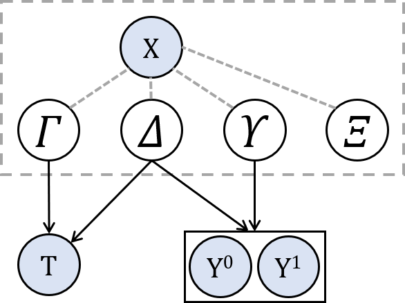
Figure 1: The three underlying factors of an observational data (namely $\Gamma$, $\Delta$, and $\Upsilon$) (Hassanpour and Greiner, 2020). $\Xi$ represents noise.

2 Related Works

For notation, we will use $x$ to describe an instance, and let $t\in\{0,1\}$ refer to the treatment administered, yielding the outcome with value $y\in{\cal R}$; see Appendix A for details.

CFR-Net     Shalit et al. (2017) considered the binary treatment task and attempted to learn a representation space $\Phi$ that reduces selection bias by making $\textrm{Pr}(\,\Phi(x)\,|\,t\!=\!0\,)$ and $\textrm{Pr}(\,\Phi(x)\,|\,t\!=\!1\,)$ as close to each other as possible, provided that $\Phi(\,x\,)$ retains enough information that the learned regressors $\{\,h^{t}\big{(}\Phi(\cdot)\big{)}\,:\ t\!\in\!\{0,1\}\,\}$ can generalize well on the observed outcomes. Their objective function includes $\ L\big{[}\,y_{i},\,h^{t_{i}}\big{(}\Phi(x_{i})\big{)}\big{]}$, which is the loss of predicting the observed outcome for instance $i$ (described as $x_{i}$), weighted by $\omega_{i}=\frac{t_{i}}{2u}+\frac{1-t_{i}}{2(1-u)}$, where $u=\textrm{Pr}(\,t\!=\!1\,)$. This is effectively setting $\omega_{i}=\frac{1}{2\,\textrm{Pr}(\,t_{i}\,)}$ where $\textrm{Pr}(\,t_{i}\,)$ is the probability of selecting treatment $t_{i}$ over the entire population.

DR-CFR     Hassanpour and Greiner (2020) argued against the standard implicit assumption that all of the covariates $X$ are confounders (i.e., contributing to both treatment assignment and outcome determination). Instead, they proposed the graphical model shown in Figure 1 (with the underlying factors $\Gamma$, $\Delta$, and $\Upsilon$) and designed a discriminative causal inference approach accordingly. Specifically, their “Disentangled Representations for CFR” (DR-CFR) model includes three representation networks, each trained with constraints to ensure that each component corresponds to its respective underlying factor. While the idea behind DR-CFR provides an interesting intuition, it is known that only generative models (and not discriminative ones) can truly identify the underlying data generating mechanism. This paper is a step in this direction.

Dragon-Net     Shi et al. (2019)’s main objective was to estimate the Average Treatment Effect (ATE), which they explain requires a two stage procedure: (i) fit models that predict the outcomes for each treatment; and (ii) find a downstream estimator of the effect. Their method is based on a classic result from strong ignorability (i.e., Theorem 3 in (Rosenbaum and Rubin, 1983)) that states:

$$(y^{1},y^{0})\mathchoice{\mathrel{\hbox to0.0pt{$\displaystyle\perp$\hss}\mkern 2.0mu{\displaystyle\perp}}}{\mathrel{\hbox to0.0pt{$\textstyle\perp$\hss}\mkern 2.0mu{\textstyle\perp}}}{\mathrel{\hbox to0.0pt{$\scriptstyle\perp$\hss}\mkern 2.0mu{\scriptstyle\perp}}}{\mathrel{\hbox to0.0pt{$\scriptscriptstyle\perp$\hss}\mkern 2.0mu{\scriptscriptstyle\perp}}}t\,|\,x \& \quad\textrm{Pr}(\,t=1\,|\,x\,) \in(0,1) \implies$$

$$(y^{1},y^{0})\mathchoice{\mathrel{\hbox to0.0pt{$\displaystyle\perp$\hss}\mkern 2.0mu{\displaystyle\perp}}}{\mathrel{\hbox to0.0pt{$\textstyle\perp$\hss}\mkern 2.0mu{\textstyle\perp}}}{\mathrel{\hbox to0.0pt{$\scriptstyle\perp$\hss}\mkern 2.0mu{\scriptstyle\perp}}}{\mathrel{\hbox to0.0pt{$\scriptscriptstyle\perp$\hss}\mkern 2.0mu{\scriptscriptstyle\perp}}}t\,|\,b(x) \& \quad\textrm{Pr}(\,t=1\,|\,b(x)\,) \in(0,1)$$

where $b(x)$ is a balancing score (here, propensity) and argued that only the parts of $X$ relevant for predicting $T$ are required for the estimation of the causal effect. This theorem only provides a way to match treated and control instances though — i.e., it helps finding potential counterfactuals from the alternative group, which they use to calculate ATE. Shi et al. (2019), however, used this theorem to derive minimal representations on which to regress to estimate the outcomes.

GANITE     Yoon et al. (2018) proposed the counterfactual GAN, whose generator $G$, given $\{x,t,y^{t}\}$, estimates the counterfactual outcomes ($\hat{y}^{\neg t}$); and whose discriminator $D$ tries to identify which of $\{[x,0,y^{0}],\ [x,1,y^{1}]\}$ is the factual outcome. It is, however, unclear why this requires that $G$ must produce samples that are indistinguishable from the factual outcomes, especially as $D$ can just learn the treatment selection mechanism (i.e.,  the mapping from $X$ to $T$) instead of distinguishing the factual outcomes from counterfactuals. Although this work is among the few generative approaches for causal inference, our empirical results (in Section 4) show that it does not effectively estimate counterfactual outcomes.

CEVAE     Louizos et al. (2017) used VAE to extract latent confounders from their observed proxies in $X$. While this is a step in the right direction, empirical results show that it does not always accurately estimate treatment effects (see Section 4). The authors note that this may be because CEVAE is not able to address the problem of selection bias. Another reason for CEVAE’s sub-optimal performance might be its assumed graphical model of the underlying data generating mechanism, depicted in Figure 2. This model assumes that there is only one latent variable $Z$ (confounding $T$ and $Y$) that generates the entire observational data; however, (Kuang et al., 2017; Hassanpour and Greiner, 2020) have shown the advantages of involving more factors (see Figure 1).

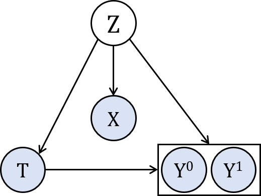
Figure 2: Graphical model of the CEVAE method (Louizos et al., 2017)

TEDVAE     Similar to DR-CFR (Hassanpour and Greiner, 2020), Zhang et al. (2021) proposed TEDVAE in an attempt to learn disentangled factors but using a generative model instead (i.e., a VAE with a three-headed encoder, one for each underlying factor). While their method proposed an interesting intuition on how to achieve this task, according to the reported empirical results (see their Figure 4c), the authors found that TEDVAE is not successful in identifying the risk factors $z_{y}$ (equivalent to our $\Upsilon$). This might be because their model does not have a mechanism for distinguishing between the risk factors and confoundings $z_{c}$ (equivalent to our $\Delta$). The evidence is in their Equation (8), which would allow $z_{y}$ to be degenerate and have all information embedded in $z_{c}$. Our work, however, proposes an architecture that can achieve this decomposition.

M1 and M2 VAEs     The M1 model (Kingma and Welling, 2014) is the conventional VAE, which learns a latent representation from the covariate matrix $X$ alone in an unsupervised manner. Kingma et al. (2014) extended this to the M2 model that, in addition to the covariates, also allows the target information to guide the representation learning process in a semi-supervised manner. Stacking the M1 and M2 models produced their best results: first learn a representation $Z_{1}$ from the raw covariates, then find a second representation $Z_{2}$, now learning from $Z_{1}$ (instead of the raw data) as well as the target information. Appendix B.1 presents a more detailed overview of the M1 and M2 VAEs. In our work, the target information includes the treatment bit $T$ as well as the observed outcome $Y$. This additional information helps the model to learn more expressive representations, which was not possible with the unsupervised M1 model.

3 Method

Following (Kuang et al., 2017; Hassanpour and Greiner, 2020) and without loss of generality, we assume that $X$ follows an unknown joint probability distribution $\textrm{Pr}(\,X\,|\,\Gamma,\Delta,\Upsilon,\Xi\,)$, where $\Gamma$, $\Delta$, $\Upsilon$, and $\Xi$ are non-overlapping independent factors. Moreover, we assume that the treatment $T$ follows $\textrm{Pr}(\,T\,|\,\Gamma,\Delta\,)$ (i.e., $\Gamma$ and $\Delta$ are responsible for selection bias) and the outcome $Y^{{}^{T}}$ follows $\textrm{Pr}_{{}_{T}}(\,Y^{{}^{T}}\,|\,\Delta,\Upsilon\,)$ — see Figure 1. Observe that the factor $\Gamma$ (respectively, $\Upsilon$) partially determines only $T$ (respectively, $Y$), but not $Y$ (respectively, $T$); and $\Delta$ includes the confounding factors between $T$ and $Y$.

We emphasize that the belief net in Figure 1 is built without loss of generality; i.e., it also covers the scenarios where any of the latent factors is degenerate. Therefore, if we can design a method that has the capacity to capture all of these latent factors, it would be successful in all scenarios — even in the ones that have degenerate factors (and in fact this is true; see the experimental setting and results of the Synthetic benchmark in Sections 4.1 and 4.3).

Our goal is to design a generative model architecture that encourages learning decomposed representations of these underlying latent factors (see Figure 1). In other words, it should be able to decompose and separately learn the three underlying factors that are responsible for determining “$T$ only” ($\Gamma$), “$Y$ only” ($\Upsilon$), and “both $T$ and $Y$” ($\Delta$). To achieve this, we propose a progressive sequence of three models (namely Series, Parallel, and Hybrid; as illustrated in Figures 3(a), 3(b), and 3(c) respectively), where each is an improvement over the previous one. Every model employs several stacked M1+M2 VAEs (Kingma et al., 2014), that each includes a decoder (generative model) and an encoder (variational posterior), which are parametrized as deep neural networks.

(a) The Series Model

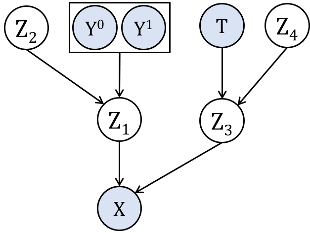
(b) The Parallel Model

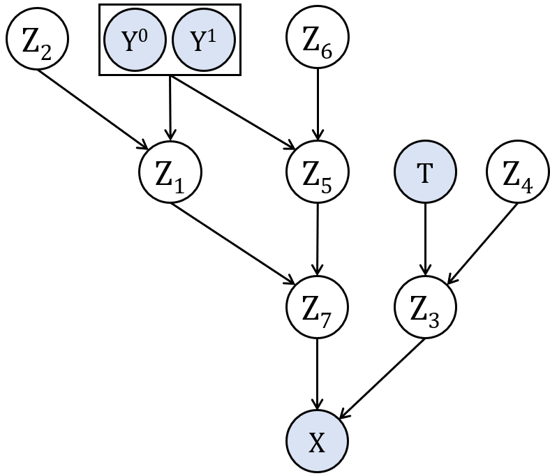
(c) The Hybrid Model

Figure 3: Belief nets of the proposed models.

3.1 The Variational Auto-Encoder Component

3.1.1 The Series Model

The belief net of the Series model is illustrated in Figure 3(a). Louizos et al. (2015) proposed a similar architecture to address fairness in machine learning, but using a binary sensitive variable $S$ (e.g., gender, race, etc.) rather than the treatment $T$. Here, we employ this architecture for causal inference and explain why it should work. We hypothesize that this structure functions as a fractionating column: the bottom M2 VAE attempts to decompose $\Gamma$ (guided by $T$) from $\Delta$ and $\Upsilon$ (captured by $Z_{1}$); and the top M2 VAE attempts to learn $\Delta$ and $\Upsilon$ (guided by $Y$).

The decoder and encoder components of the Series model — $p(\cdot)$ and $q(\cdot)$ parametrized by $\theta_{s}$ and $\phi_{s}$ respectively — involve the following distributions:

Priors		Likelihood	Posteriors
$p_{\theta_{s}}(z_{2})$	$p_{\theta_{s}}(z_{1}|y,z_{2})$	$p_{\theta_{s}}(x|z_{1},t)$	$q_{\phi_{s}}(z_{1}|x,t)$	$q_{\phi_{s}}(y|z_{1})$
			$q_{\phi_{s}}(z_{2}|y,z_{1})$

Hereafter, we drop the $\theta$ and $\phi$ subscripts for brevity.

The goal is to maximize the conditional log-likelihood of the observed data (left-hand-side of the following inequality) by maximizing the Evidence Lower BOund (ELBO; right-hand-side) — i.e.,

$$\sum_{i=1}^{N}\log p(x_{i}|t_{i},y_{i})\quad\geq\quad\sum_{i=1}^{N}\mathbb{E}_{q(z_{1}|x,t)}\big{[}\log p(x_{i}|z_{1_{i}},t_{i})\big{]}$$ (1)

$$-\textrm{KL}\big{(}\,q(z_{1}|x,t)\ ||\ p(z_{1}|y,z_{2})\,\big{)}-\textrm{KL}\big{(}\,q(z_{2}|y,z_{1})\ ||\ p(z_{2})\,\big{)}$$ (2)

where KL denotes the Kullback-Leibler divergence, $p(z_{2})$ is the unit multivariate Gaussian (i.e., $\mathcal{N}(0,\mathbb{I})$), and the other distributions are parameterized as deep neural networks.

3.1.2 The Parallel Model

The Series model is composed of two M2 stacked models. However, Kingma et al. (2014) showed that an M1+M2 stacked architecture learns better representations than an M2 model alone for a downstream prediction task. This motivated us to design a double M1+M2 Parallel model; where one arm is for the outcome to guide the representation learning via $Z_{1}$ and another for the treatment to guide the representation learning via $Z_{3}$. Figure 3(b) shows the belief net of this model. We hypothesize that $Z_{1}$ would learn $\Delta$ and $\Upsilon$, and $Z_{3}$ would learn $\Gamma$ (and perhaps partially $\Delta$).

The decoder and encoder components of the Parallel model — $p(\cdot)$ and $q(\cdot)$ parametrized by $\theta_{p}$ and $\phi_{p}$ respectively — involve the following distributions:

Priors		Likelihood	Posteriors
$p(z_{2})$	$p(z_{1}|y,z_{2})$	$p(x|z_{1},z_{3})$	$q(z_{1}|x,t)$	$q(y|z_{1})$
$p(z_{4})$	$p(z_{3}|t,z_{4})$		$q(z_{2}|y,z_{1})$	$q(t|z_{3})$
			$q(z_{3}|x,y)$
			$q(z_{4}|t,z_{3})$

Here, the conditional log-likelihood can be upper bounded by:

$$\sum_{i=1}^{N}\log p(x_{i}|t_{i},y_{i})\quad\geq\quad\sum_{i=1}^{N}\mathbb{E}_{q(z_{1},z_{3}|x,t,y)}\big{[}\log p(x_{i}|z_{1_{i}},z_{3_{i}})\big{]}$$ (3)

$$-\textrm{KL}\big{(}\,q(z_{1}|x,t)\ ||\ p(z_{1}|y,z_{2})\,\big{)}-\textrm{KL}\big{(}\,q(z_{2}|y,z_{1})\ ||\ p(z_{2})\,\big{)}$$

$$-\textrm{KL}\big{(}\,q(z_{3}|x,y)\ ||\ p(z_{3}|t,z_{4})\,\big{)}-\textrm{KL}\big{(}\,q(z_{4}|t,z_{3})\ ||\ p(z_{4})\,\big{)}$$ (4)

3.1.3 The Hybrid Model

The final model, Hybrid (see Figure 3(c)), attempts to combine the best capabilities of the previous two architectures. The backbone of the Hybrid model has a Series architecture, that separates $\Gamma$ (factors related to the treatment $T$; captured by the right module with $Z_{3}$ as its head) from $\Delta$ and $\Upsilon$ (factors related to the outcome $Y$; captured by the left module with $Z_{7}$ as its head). The left module, itself, consists of a Parallel model that attempts to proceed one step further and decompose $\Delta$ from $\Upsilon$. This is done with the help of a discrepancy penalty (see Section 3.3).

The decoder and encoder components of the Hybrid model — $p(\cdot)$ and $q(\cdot)$ parametrized by $\theta_{h}$ and $\phi_{h}$ respectively — involve the following distributions:

Priors		Likelihood	Posteriors
$p(z_{2})$	$p(z_{1}|y,z_{2})$	$p(x|z_{3},z_{7})$	$q(z_{1}|z_{7})$	$q(y|z_{1},z_{5})$
$p(z_{4})$	$p(z_{3}|t,z_{4})$		$q(z_{2}|y,z_{1})$	$q(t|z_{3})$
$p(z_{6})$	$p(z_{5}|y,z_{6})$		$q(z_{3}|x,y)$
	$p(z_{7}|z_{1},z_{5})$		$q(z_{4}|t,z_{3})$
			$q(z_{5}|z_{7})$
			$q(z_{6}|y,z_{5})$
			$q(z_{7}|x,t)$

Here, the conditional log-likelihood can be upper bounded by:

$$\sum_{i=1}^{N}\log p(x_{i}|t_{i},y_{i})\quad\geq\quad\sum_{i=1}^{N}\mathbb{E}_{q(z_{3},z_{7}|x,t,y)}\big{[}\log p(x_{i}|z_{3_{i}},z_{7_{i}})\big{]}$$ (5)

$$-\textrm{KL}\big{(}\,q(z_{1}|z_{7})\ ||\ p(z_{1}|y,z_{2})\,\big{)}-\textrm{KL}\big{(}\,q(z_{2}|y,z_{1})\ ||\ p(z_{2})\,\big{)}$$

$$-\textrm{KL}\big{(}\,q(z_{3}|x,y)\ ||\ p(z_{3}|t,z_{4})\,\big{)}-\textrm{KL}\big{(}\,q(z_{4}|t,z_{3})\ ||\ p(z_{4})\,\big{)}$$

$$-\textrm{KL}\big{(}\,q(z_{5}|z_{7})\ ||\ p(z_{5}|y,z_{6})\,\big{)}-\textrm{KL}\big{(}\,q(z_{6}|y,z_{5})\ ||\ p(z_{6})\,\big{)}$$

$$-\textrm{KL}\big{(}\,q(z_{7}|x,t)\ ||\ p(z_{7}|z_{1},z_{5})\,\big{)}$$ (6)

For all three of these models, we refer to the first term in the ELBO (i.e., right-hand-side of Equations (1), (3), or (5)) as the Reconstruction Loss (RecL) and the next term(s) (i.e., Equations (2), (4), or (6)) as the KL Divergence (KLD). Concisely, the ELBO can be viewed as maximizing: $\textrm{RecL}-\textrm{KLD}$.

3.2 Further Disentanglement with $\beta$-VAE

As mentioned earlier, we want the learned latent variables to be disentangled, to match our assumption of non-overlapping factors $\Gamma$, $\Delta$, and $\Upsilon$. To encourage this, we employ the $\beta$-VAE (Higgins et al., 2017), which adds a hyperparameter $\beta$ as a multiplier of the KLD part of the ELBO. This adjustable hyperparameter facilitates a trade-off that helps balance the latent channel capacity and independence constraints with the reconstruction accuracy — i.e., including the $\beta$ hyperarameter should grant a better control over the level of disentanglement in the learned representations (Burgess et al., 2018). Therefore, the generative objective to be minimized becomes:

$$\begin{split}\mathcal{L}_{\textrm{VAE}}\quad=\quad-\textrm{RecL}\;+\;\beta\cdot\textrm{KLD}\end{split}$$ (7)

Although Higgins et al. (2017) suggest setting $\beta$ greater than $1$ in most applications, Hoffman et al. (2017) show that having a $\beta<1$ weight on the KLD term can be interpreted as optimizing the ELBO under an alternative prior, which functions as a regularization term to reduce the chance of degeneracy.

3.3 Discrepancy

Although all three proposed models encourage statistical independence between $T$ and $Z_{1}$ in the marginal posterior $q_{\phi}(Z_{1}|T)$ where $X$ is not given — see the collider structure (at $X$): $T~{}\rightarrow~{}X~{}\leftarrow~{}Z_{1}$ in Figure 3(a) — an information leak is quite possible due to the correlation between the outcome $Y$ and treatment $T$ in the data. We therefore require an extra regularization term on $q_{\phi}(Z_{1}|T)$ in order to penalize the discrepancy (denoted by $\mathtt{disc}$) between the conditional distributions of $Z_{1}$ given $T\!=\!0$ versus given $T\!=\!1$. To achieve this regularization, we calculate the $\mathtt{disc}$ using an Integral Probability Metric (IPM) (Mansour et al., 2009) (cf., (Louizos et al., 2015; Shalit et al., 2017; Yao et al., 2018), etc.) that measures the distance between the two above-mentioned distributions:

$$\mathcal{L}_{\mathtt{disc}}\quad=\quad\textrm{IPM}\big{(}\ \{z_{1}\}_{i:t_{i}=0},\ \{z_{1}\}_{i:t_{i}=1}\ \big{)}$$ (8)

3.4 Predictive Loss

Note, however, that neither the VAE nor the $\mathtt{disc}$ losses contribute to training a predictive model for outcomes. To remedy this, we extend the objective function to include a discriminative term for the regression loss of predicting $y$:

$$\mathcal{L}_{\textrm{pred}}\quad=\quad\frac{1}{N}\sum_{i=1}^{N}\omega_{i}\cdot\mathcal{L}\big{[}\,y_{i},\,\hat{y}_{i}\big{]}$$ (9)

where the predicted outcome $\hat{y}_{i}=\mathbb{E}\big{[}\,q_{\phi}^{t_{i}}(y_{i}|z_{1_{i}})\,\big{]}$; $\mathcal{L}\big{[}\,y_{i},\,\hat{y}_{i}\,\big{]}$ is the factual loss (i.e., L2 loss for real-valued outcomes and log loss for binary-valued outcomes); and $\omega_{i}$ represent the weights that attempt to account for selection bias. We consider two approaches in the literature to derive the weights: (i) the Population-Based (PB) weights as proposed in (Shalit et al., 2017); and (ii) the Context-Aware (CA) weights as proposed in (Hassanpour and Greiner, 2019). Note that disentangling $\Delta$ from $\Upsilon$ is only beneficial when using the CA weights, since we need just the $\Delta$ factors to derive them (Hassanpour and Greiner, 2020).

3.5 Final Model(s)

Putting everything together, the overall objective function to be minimized is:

$$\mathcal{J}\quad=\quad\mathcal{L}_{\textrm{pred}}\;+\;\alpha\cdot\mathcal{L}_{\mathtt{disc}}\;+\;\gamma\cdot\mathcal{L}_{\textrm{VAE}}\;+\;\lambda\cdot\mathfrak{Reg}$$ (10)

where $\mathfrak{Reg}$ penalizes the model complexity.

This objective function is motivated by the work of (McCallum et al., 2006), which suggested optimizing a convex combination of discriminative and generative losses would indeed improve predictive performance. As an empirical verification, note that for $\gamma\!=\!0$, the Series and Parallel models effectively reduce to CFR-Net. However, our empirical results (see Section 4) suggest that the generative term in the objective function helps learning representations that embed more relevant information for estimating outcomes than that of $\Phi$ in CFR-Net.

We refer to the family of our proposed methods as VAE-CI (Variational Auto-Encoder for Causal Inference); specifically: {S, P, H}-VAE-CI, for Series, Parallel, and Hybrid respectively. We anticipate that each method is an improvement over the previous one in terms of estimating causal effects, culminating in H-VAE-CI, which we expect can best decompose the underlying factors and accurately estimate the outcomes of all treatments.

4 Experiments, Results, and Discussion

4.1 Benchmarks

1. Infant Health and Development Program (IHDP)     The original IHDP randomized controlled trial was designed to evaluate the effect of specialist home visits on future cognitive test scores of premature infants. Hill (Hill, 2011) induced selection bias by removing a non-random subset of the treated population. The dataset contains 747 instances (608 control and 139 treated) with $25$ covariates. We use the same benchmark (with $100$ realizations of outcomes) provided by and used in (Johansson et al., 2016) and (Shalit et al., 2017).

2. Atlantic Causal Inference Conference 2018 (ACIC’18)     ACIC’18 is a collection of binary-treatment observational datasets released for a data challenge. Following (Shi et al., 2019), we used those datasets with $N\!\in\!\{1,5,10\}\!\times\!10^{3}$ instances (four datasets in each category). The covariates matrix for each dataset involves 177 features and is sub-sampled from a table of medical measurements taken from the Linked Birth and Infant Death Data (LBIDD) (MacDorman and Atkinson, 1998), that contains information corresponding to 100,000 subjects.

3. Fully Synthetic Datasets     We generated a set of synthetic datasets according to the procedure described in (Hassanpour and Greiner, 2020) (details in Appendix C.1). We considered all the viable datasets in a mesh generated by various sets of variables, of sizes $m_{\Gamma},m_{\Delta},m_{\Upsilon}\in\{0,4,8\}$ and $m_{\Xi}\!=\!1$. This creates $24$ scenarios that consider all relevant combinations of sizes of $\Gamma$, $\Delta$, and $\Upsilon$ (corresponding to different levels of selection bias). For each scenario, we synthesized multiple datasets with various initial random seeds to allow for statistical significance testing of the performance comparisons between the contending methods.

4.2 Identification of the Underlying Factors

4.2.1 Procedure for Evaluating Identification of the Underlying Factors

To evaluate the identification performance of the underlying factors, we use a fully synthetic dataset (#3 above) with $m_{\Gamma}\!=\!m_{\Delta}\!=\!m_{\Upsilon}\!=\!8$ and $m_{\Xi}\!=\!1$. We then ran the learned model on four dummy test instances $V_{i}\in{\cal R}^{m_{\Gamma}+m_{\Delta}+m_{\Upsilon}+m_{\Xi}}$ as depicted on the left-side of Figure 4. The first to third vectors had “1” (constant) in the positions associated with $\Gamma$, $\Delta$, and $\Upsilon$ respectively, and the remaining 17 positions were filled with “0”. The fourth vector was all “1” except for the last position (the noise) which was “0”. This helps measure the maximum amount of information that is passed to the final layer of each representation network.

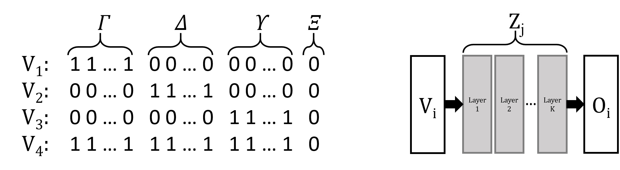
Figure 4: The four dummy $x$-like vectors (left); and the input/output vectors of the representation networks (right).

Next, each vector $V_{i}$ is fed to each trained network $Z_{j}$ (as if it was $x$). We let $O_{i,j}$ be the $\mathtt{relu}$ output (here, $\in\!{\cal R}^{200}$) of the encoder network $Z_{j}$ when $x\!=\!V_{i}$. The average of the $200$ values of the $O_{i,j}$ (i.e., $Avg(O_{i,j})$) represents the power of signal that was produced by the $Z_{j}$ channel on the input $V_{i}$. The values reported in the tables illustrated in Figure 5 are the ratios of $Avg(O_{1,j})$, $Avg(O_{2,j})$, and $Avg(O_{3,j})$ divided by $Avg(O_{4,j})$ for each of the learned representation networks. Note that, a larger ratio indicates that the respective representation network $Z_{j}$ has allowed more of the input signal $V_{i}$ to pass through.

If the model could perfectly learn each underlying factor in a disentangled manner, we expect to see one element in each column to be significantly larger than the other elements in that column. For example, for H-VAE-CI, the weights of the $\Gamma$ row should be highest for $Z_{3}$, as that means $Z_{3}$ has captured the $\Gamma$ factors. Similarly, we would want the $Z_{5}$ and $Z_{1}$ entries on the $\Delta$ and $\Upsilon$ rows to be largest respectively.

4.2.2 Results’ Analysis

As expected, Figure 5 shows that $Z_{3}$ and $Z_{4}$ capture $\Gamma$ (e.g., the $Z_{3}$ ratios for $\Gamma$ in the {P, H}-VAE-CI tables are largest), and $Z_{1}$, $Z_{2}$, $Z_{5}$, $Z_{6}$, and $Z_{7}$ capture $\Delta$ and $\Upsilon$. Note that decomposition of $\Delta$ from $\Upsilon$ has not been achieved by any of the methods except for H-VAE-CI, which captures $\Upsilon$ by $Z_{1}$ and $\Delta$ by $Z_{5}$ (note the ratios are largest for $Z_{1}$ and $Z_{5}$). This decomposition is vital for deriving context-aware importance sampling weights because they must be calculated from $\Delta$ only (Hassanpour and Greiner, 2020). Also observe that {P, H}-VAE-CI are each able to separate $\Gamma$ from $\Delta$. However, DR-CFR, which tried to disentangle all factors, failed not only to disentangle $\Delta$ from $\Upsilon$, but also $\Gamma$ from $\Delta$.

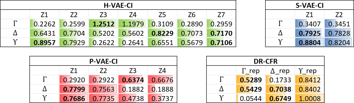
Figure 5: Performance analysis for decomposition of the underlying factors on the Synthetic dataset with $m_{\Gamma}\!=\!m_{\Delta}\!=\!m_{\Upsilon}\!=\!8$ and $m_{\Xi}\!=\!1$. (The color shading in each cell represents the value of that cell, with a larger amount of color for larger values.)

4.3 Treatment Effect Estimation

There are two categories of performance measures:

Individual-based: “Precision in Estimation of Heterogeneous Effect” (Hill, 2011):

$$\textrm{{\small PEHE}}\!=\!\sqrt{\frac{1}{N}\sum_{i=1}^{N}\left(\hat{\textrm{e}}_{i}\!-\!\textrm{e}_{i}\right)^{2}}$$ (11)

uses $\hat{\textrm{e}}_{i}=\hat{y}_{i}^{1}-\hat{y}_{i}^{0}$ as the estimated effect and $\textrm{e}_{i}=y_{i}^{1}-y_{i}^{0}$ as the true effect.

Population-based: “Bias of the Average Treatment Effect”:

$$\epsilon_{\textrm{ATE}}\!=\!\big{|}\textrm{ATE}-\widehat{\textrm{ATE}}\big{|}$$ (12)

where $\,\textrm{ATE}=\frac{1}{N}\sum_{i=1}^{N}y^{1}_{i}-\frac{1}{N}\sum_{j=1}^{N}y^{0}_{j}\,$ and $\widehat{\textrm{ATE}}$ follows the same formula except that it is calculated based on the estimated outcomes.

In this paper, we compare performances of the proposed {S, P, H}-VAE-CI versus the following treatment effect estimation methods: CFR-Net (Shalit et al., 2017), DR-CFR (Hassanpour and Greiner, 2020), Dragon-Net (Shi et al., 2019), GANITE (Yoon et al., 2018), CEVAE (Louizos et al., 2017), and TEDVAE (Zhang et al., 2021). The basic search grid for hyperparameters of the CFR-Net based algorithms (including our methods) is available in Appendix C.2. To ensure that our performance gain is not merely based on an increased complexity of the models, we also performed our grid search for all the contending methods with an updated number of layers and/or number of neurons in each layer, This guaranteed that all methods have the same number of parameters and therefore a similar model complexity.

We ran the experiments for the contender methods using their publicly available code-bases; note the following points regarding these runs:

• Since Dragon-Net is designed to estimate ATE only, we did not report its performance results for the PEHE measure (which, as expected, were significantly inaccurate).

• Original GANITE code-base could only deal with binary outcomes. We modified the code (losses, etc.) to allow it to process real-valued outcomes also.

• We were surprised that CEVAE diverged when running on the ACIC’18 datasets. To avoid this, we had to run the ACIC’18 experiments on the binary covariates only.

4.3.1 Results’ Analysis

Table 1 summarizes the mean and standard deviation of the PEHE and $\epsilon_{\textrm{ATE}}$ measures (lower is better) on the IHDP, ACIC’18, and Synthetic benchmarks. VAE-CI achieves the best performance among the contending methods. These results are statistically significant (in bold; based on the Welch’s unpaired t-test with $\alpha\!=\!0.05$) for the IHDP and Synthetic benchmarks. Although VAE-CI also achieves the best performance on the ACIC’18 benchmark, the results are not statistically significant due to the high standard deviation of the performances of the contending methods.

Table 1: PEHE and $\epsilon_{\textrm{ATE}}$ performance measures (lower is better) represented in the form of “mean (standard deviation)”. The bold values in each column are the best (statistically significant based on the Welch’s unpaired t-test with $\alpha\!=\!0.05$).

Method	IHDP		ACIC’18		Synthetic
	PEHE	$\epsilon_{\textrm{ATE}}$	PEHE	$\epsilon_{\textrm{ATE}}$	PEHE	$\epsilon_{\textrm{ATE}}$
CFR-Net	0.75 (0.57)	0.08 (0.10)	5.13 (5.59)	1.21 (1.81)	0.39 (0.08)	0.027 (0.020)
DR-CFR	0.65 (0.37)	0.03 (0.04)	3.86 (3.39)	0.80 (1.41)	0.26 (0.07)	0.007 (0.004)
Dragon-Net	NA	0.14 (0.15)	NA	0.48 (0.77)	NA	0.007 (0.005)
GANITE	2.81 (2.30)	0.24 (0.46)	3.55 (2.27)	0.69 (0.65)	1.28 (0.43)	0.036 (0.015)
CEVAE	2.50 (3.47)	0.18 (0.25)	5.30 (5.52)	3.29 (3.50)	1.39 (0.32)	0.287 (0.217)
TEDVAE	1.61 (2.37)	0.18 (0.23)	6.63 (8.69)	3.74 (5.00)	0.25 (0.07)	0.013 (0.007)
S-VAE-CI	0.51 (0.37)	0.00 (0.02)	2.73 (2.39)	0.51 (0.82)	0.28 (0.05)	0.004 (0.003)
P-VAE-CI	0.52 (0.36)	0.01 (0.03)	2.62 (2.26)	0.37 (0.75)	0.28 (0.05)	0.004 (0.003)
H-VAE-CI (PB)	0.49 (0.36)	0.01 (0.02)	1.78 (1.27)	0.44 (0.77)	0.20 (0.03)	0.003 (0.002)
H-VAE-CI (CA)	0.48 (0.35)	0.01 (0.01)	1.66 (1.30)	0.39 (0.75)	0.18 (0.02)	0.003 (0.002)

Figure 6 visualizes the PEHE measures on the entire synthetic datasets with sample size of $N\!=\!10,\!000$. We observe that both plots corresponding to H-VAE-CI method (PB as well as CA) are completely within the plots of all other methods, showcasing H-VAE-CI’s superior performance under every possible selection bias scenario. Note that for scenarios where $m_{\Delta}\!=0$ (i.e.,  the ones of the form $m_{\Gamma}$_$0$_$m_{\Upsilon}$ on the perimeter of the radar chart in Figure 6), the performances of H-VAE-CI (PB) and H-VAE-CI (CA) are almost identical. This is expected, since for these scenarios, the learned representation for $\Delta$ would be degenerate, and therefore, the context-aware weights would reduce to population-based ones. On the other hand, for scenarios where $m_{\Delta}\!\neq 0$, the H-VAE-CI (CA) often performs better than H-VAE-CI (PB). This may be because H-VAE-CI has correctly disentangled $\Delta$ from $\Upsilon$. This facilitates learning good CA weights that better account for selection bias, which in turn, results in a better causal effect estimation performance.

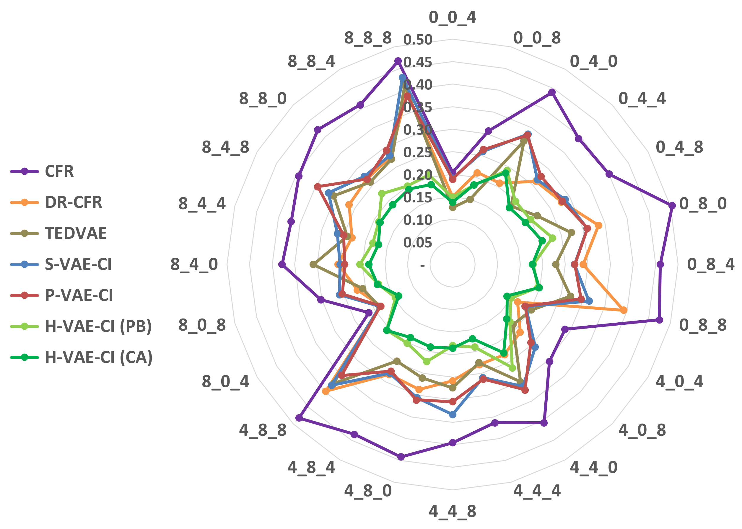
Figure 6: Radar graphs of PEHE (on the radii; closer to the center is better) for the entire Synthetic benchmark ($24\times 3$ with $N\!=\!10,\!000$; each vertex denotes the respective dataset). Figure is best viewed in color.

4.4 Hyperparameters’ Sensitivity Analyses

Figure 7 illustrates the results of our hyperparameters’ sensitivity analyses (in terms of PEHE). In the following, we discuss the insights we gained from these ablation studies:

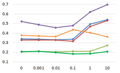
(a) $\alpha$

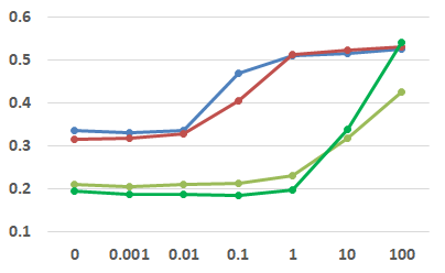
(b) $\beta$

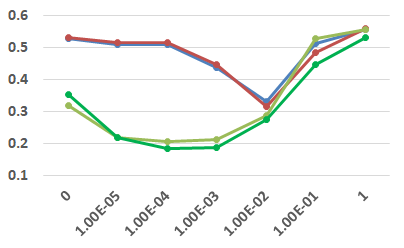
(c) $\gamma$

Figure 7: Hyperparameters’ ($x$-axis) sensitivity analysis based on PEHE ($y$-axis) on the synthetic dataset with $m_{\Gamma,\Delta,\Upsilon}\!=\!8,m_{\Xi}\!=\!1$. Legend is the same as Figure 6: purple for CFR-Net, orange for DR-CFR, blue for S-VAE-CI, red for P-VAE-CI, and light and dark green for H-VAE-CI (PB) and (CA) respectively. Plots are best viewed in color.

• For the $\alpha$ hyperparameter (i.e., coefficient of the discrepancy penalty), Figure 7(a) suggests that DR-CFR and H-VAE-CI methods have the most robust performance throughout various values of $\alpha$. This is expected, because, unlike CFR-Net and {S, P}-VAE-CI, DR-CFR and H-VAE-CI possess an independent node for representing $\Delta$. This helps them still capture $\Delta$ as $\alpha$ grows; since for them, $\alpha$ only affects learning a representation of $\Upsilon$. Comparing H-VAE-CI (PB) with (CA), we observe that for all $\alpha\!>\!0.01$, (CA) outperforms (PB). This is because the discrepancy penalty would force $Z_{1}$ to only capture $\Upsilon$ and $Z_{5}$ to only capture $\Delta$. This results in deriving better CA weights (that should be learned from $\Delta$; here, from its learned representation $Z_{5}$). H-VAE-CI (PB), on the other hand, cannot take advantage of this disentanglement, which explains its sub-optimal performance.

• Figure 7(b) shows that various $\beta$ values (i.e., coefficient of KL divergence penalty) do not make much difference for H-VAE-CI (except for $\beta\geq 1$, since this large value means the learned representations will be close to Gaussian noise). We initially thought using $\beta$-VAE might help further disentangle the underlying factors. However, Figure 7(b) suggests that close-to-zero or even zero $\beta$s also work effectively. Our hypothesis is that the H-VAE-CI’s architecture already takes care of decomposing the $\Gamma$, $\Delta$, and $\Upsilon$ factors, without needing the help of a KLD penalty. Appendix D.1 includes more evidence and a detailed discussion on why this interpretation should hold.

• For hyperparameter $\gamma$ (i.e.,  coefficient of the generative loss penalty), H-VAE-CI achieves the most stable performance compared to the {S, P}-VAE-CI models — see Figure 7(c). Finding that H-VAE-CI for $\gamma\leq 0.01$ performs better than {S, P}-VAE-CI, suggests that having the generative loss term (i.e.,  $\mathcal{L}_{\textrm{VAE}}$) is more important for {S, P}-VAE-CI than for H-VAE-CI to perform well — note an extreme case happens at $\gamma=0$, where the latter performs significantly (statistically) better than the former. We hypothesize that this is because H-VAE-CI already learns expressive representations $Z_{3}$ and $Z_{7}$, meaning the optimization no longer really requires the $\mathcal{L}_{\textrm{VAE}}$ term to impose that. This is in contrast to $Z_{1}$ in S-VAE-CI, and $Z_{1}$ and $Z_{3}$ in P-VAE-CI.

5 Future works and Conclusion

Despite the success of the proposed methods, especially the Hybrid model, in addressing causal inference for treatment effect estimation, no known algorithms can yet learn to perfectly decompose factors $\Delta$ and $\Upsilon$. This goal is important because isolating $\Delta$, and learning Context-Aware (CA) weights from it, does enhance the quality of the causal effect estimation performance — note the superior performance of H-VAE-CI (CA). The results of our ablation study in Figure 7(b), however, revealed that the currently used $\beta$-VAE does not help much with disentanglement of the underlying factors. Therefore, the proposed architectures and objective function ought to be responsible for most of the achieved decomposition. A future direction is to explore the use of better disentangling constraints (e.g.,  works of (Chen et al., 2018) and (Lopez et al., 2018)) to see if that would yield sharper results.

The goal of this paper was to estimate causal effects (either for individuals or the entire population) from observational data. We designed three models that employ Variational Auto-Encoders (VAE) (Kingma and Welling, 2014; Rezende et al., 2014), namely Series, Parallel, and Hybrid. Each model was an improvement over the previous one, in terms of identifying the underlying factors of any observational data as well as estimating the causal effects. Our proposed methods employed Kingma et al. (2014)’s M1 and M2 models as their building blocks. Our Hybrid model performed best, and succeeded at learning decomposed representations of the underlying factors; this, in turn, helped to accurately estimate the outcomes of all treatments. Our empirical results demonstrated the superiority of the proposed methods, compared to both state-of-the-art discriminative as well as generative approaches in the literature.

Appendix A Causal Inference: Problem Setup and Challenges

A dataset $\mathcal{D}=\left\{\ [x_{i},\,t_{i},\,y_{i}]\ \right\}_{i=1}^{N}$ used for treatment effect estimation has the following format: for the $i^{th}$ instance (e.g., patient), we have some context information $x_{i}\in\mathcal{X}\subseteq{\cal R}^{K}$ (e.g., age, BMI, blood work, etc.), the administered treatment $t_{i}$ chosen from a set of treatment options $\mathcal{T}$ (e.g., {$0$: medication, $1$: surgery}), and the associated observed outcome $y_{i}\in\mathcal{Y}$ (e.g., survival time: $\mathcal{Y}\subseteq{\cal R}^{+}$) as a result of receiving treatment $t_{i}$.

Note that $\mathcal{D}$ only contains the outcome of the administered treatment (aka observed outcome: $y_{i}$), but not the outcome(s) of the alternative treatment(s) (aka counterfactual outcome(s); that is, $y_{i}^{t}$ for $t\in\mathcal{T}\setminus\{t_{i}\}$ ), which are inherently unobservable [Holland, 1986]. In other words, the causal effect $y_{i}^{1}-y_{i}^{0}$ is never observed (i.e., missing in any training data) and cannot be used to train predictive models, nor can it be used to evaluate a proposed model. This makes estimating causal effects a more difficult problem than that of generalization in the supervised learning paradigm.

Pearl [Pearl, 2009] demonstrates that, in general, causal relationships can only be learned by experimentation (on-line exploration), or running a Randomized Controlled Trial (RCT), where the treatment assignment $T$ does not depend on the individual $X$ – see Figure 8(a). In many cases, however, collecting RCT data is expensive, unethical, or even infeasible.

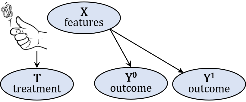
(a) Randomized Controlled Trial

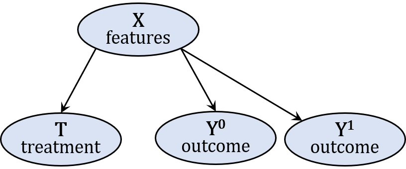
(b) Observational Study

Figure 8: Belief net structure for randomized controlled trials (a) and observational studies (b). Here, $Y^{0}$ ($Y^{1}$) is the outcome of applying $T\!=$ treatment#0 (#1) to the individual represented by $X$.

A solution is to approximate treatment effects from off-line datasets collected through Observational Studies. In such datasets, however, the administered treatment $T$ depends on some or all attributes of individual $X$ – see Figure 8(b). Here, as $\textrm{Pr}(\,T\,|\,X\,)\neq\textrm{Pr}(\,T\,)$, we say these datasets exhibit selection bias [Imbens and Rubin, 2015]. Figure 9 illustrates selection bias in an example (synthetic) observational dataset. Here, to treat heart disease, a doctor typically prescribes surgery $(t\!=\!1)$ to younger patients ($\bullet$) and medication $(t\!=\!0)$ to older ones (+). Note that instances with larger (resp., smaller) $x$ values have a higher chance to be assigned to the $t\!=\!$ 0 (resp., 1) treatment arm; hence we have selection bias. The counterfactual outcomes (only to be used for evaluation purpose) are illustrated by small fainted $\bullet$ (+) for $\neg t\!=\!$ 1 (0).

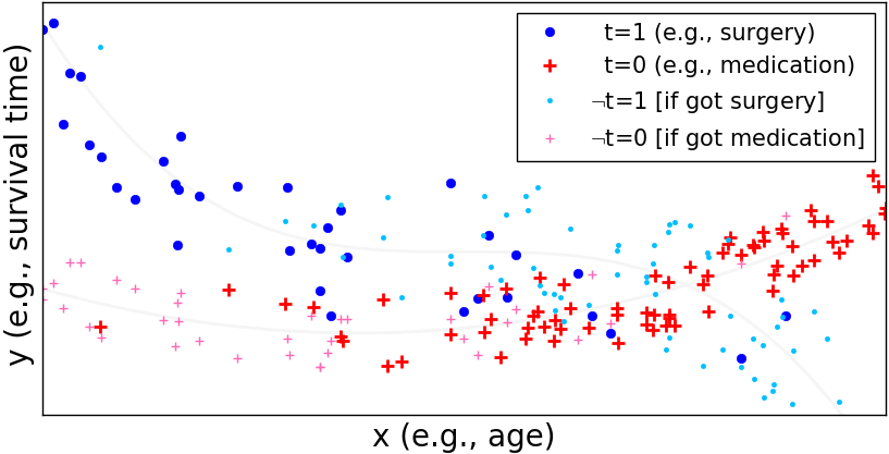
Figure 9: An example observational dataset.

Appendix B Background

B.1 M1 and M2 Variational Auto-Encoders

As the first proposed model, the M1 VAE is the conventional model that is used to learn representations of data [Kingma and Welling, 2014, Rezende et al., 2014]. These features are learned from the covariate matrix $X$ only. Figure 10(a) illustrates the decoder and encoder of the M1 VAE. Note the graphical model on the left depicts the decoder; and the one on the right depicts the encoder, which has arrows going the other direction.

Proposed by [Kingma et al., 2014], the M2 model was an attempt to incorporate the information in target $Y$ into the representation learning procedure. This results in learning representations that separate specifications of individual targets from general properties shared between various targets. In case of digit generation, this translates into separating specifications that distinguish each digit from writing style or lighting condition. Figure 10(b) illustrates the decoder and encoder of the M2 VAE.

We found that stacking the M1 and M2 models, as shown in Figure 10(c), produced the best results. This way, we can first learn a representation $Z_{1}$ from raw covariates, then find a second representation $Z_{2}$, now learning from $Z_{1}$ instead of the raw data.

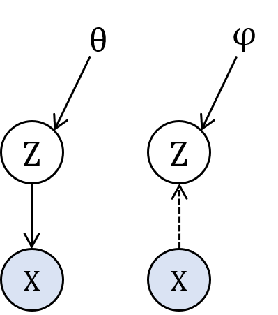
(a) M1 model

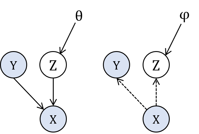
(b) M2 model

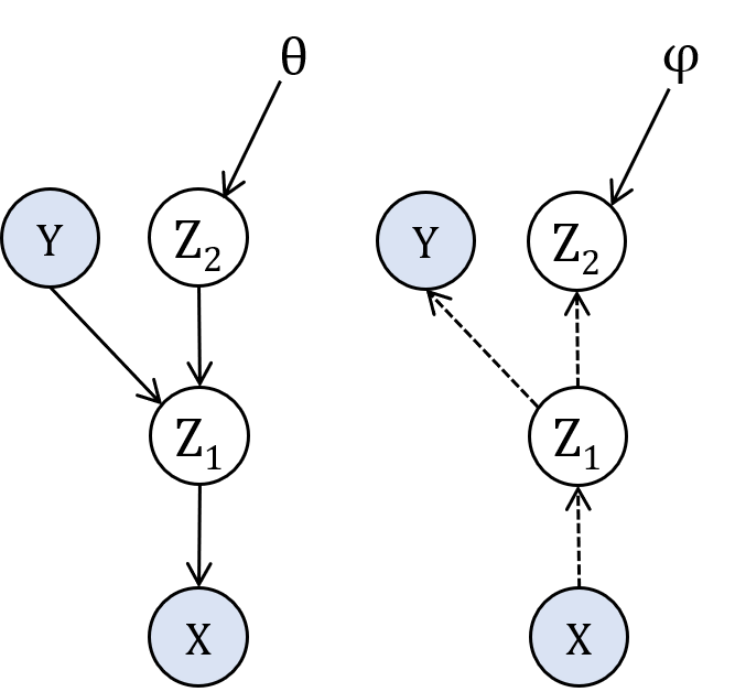
(c) M1+M2 model

Figure 10: Decoders (parametrized by $\theta$) and encoders (parametrized by $\varphi$) of the M1, M2, and M1+M2 VAEs.

Appendix C Experimental Setup

C.1 Procedure of Generating the Synthetic Datasets

Given as input the sample size $N$; dimensionalities $[m_{\Gamma},m_{\Delta},m_{\Upsilon}]\in({\cal Z}^{\geq 0})^{3}$; for each factor $L\in\{\,\Gamma,\Delta,\Upsilon\,\}$, the means and covariance matrices $(\mu_{L},\Sigma_{L})$; and a scalar $\zeta$ that determines the slope of the logistic curve.

• For each latent factor $L\in\{\,\Gamma,\Delta,\Upsilon\,\}$, form $L$ by drawing $N$ instances (each of size $m_{L}$) from $\mathcal{N}(\mu_{L},\Sigma_{L})$. The covariates matrix $X$ is the result of concatenating $\Gamma$, $\Delta$, and $\Upsilon$. Refer to the concatenation of $\Gamma$ and $\Delta$ as $\Psi$ and that of $\Delta$ and $\Upsilon$ as $\Phi$ (for later use).

• For treatment $T$, sample $m_{\Gamma}\!+\!m_{\Delta}$ tuple of coefficients $\theta$ from $\mathcal{N}(0,1)^{m_{\Gamma}\!+\!m_{\Delta}}$. Define the logging policy as $\pi_{0}(\,t\!=\!1\,|\,z\,)\ =\ \frac{1}{1+\textrm{exp}(-\zeta z)}$, where $z=\Psi\cdot\theta$. For each instance $x_{i}$, sample treatment $t_{i}$ from the Bernoulli distribution with parameter $\pi_{0}(\,t\!=\!1\,|\,z_{i}\,)$.

• For outcomes $Y^{0}$ and $Y^{1}$, sample $m_{\Delta}\!+\!m_{\Upsilon}$ tuple of coefficients $\vartheta^{0}$ and $\vartheta^{1}$ from $\mathcal{N}(0,1)^{m_{\Delta}\!+\!m_{\Upsilon}}$ Define $\;y^{0}=(\Phi\circ\Phi\circ\Phi+0.5)\cdot\vartheta^{0}/(m_{\Delta}\!+\!m_{\Upsilon})+\varepsilon\;$ and $\;y^{1}=(\Phi\circ\Phi)\cdot\vartheta^{1}/(m_{\Delta}\!+\!m_{\Upsilon})+\varepsilon$, where $\varepsilon$ is a white noise sampled from $\mathcal{N}(0,0.1)$ and $\circ$ is the symbol for element-wise product.

C.2 Hyperparameters

For all CFR, DR-CFR, and VAE-CI methods, we trained the neural networks with 3 layers (each consisting of 200 hidden neurons), non-linear activation function $\,\mathtt{elu}\,$, regularization coefficient of $\lambda$=1E-4, $\,\mathtt{Adam}\,$ optimizer [Kingma and Ba, 2015] with a learning rate of 1E-3, batch size of 300, and maximum number of iterations of $10,000$. See Table 2 for our hyperparameter search space.

Table 2: Hyperparameters and ranges

Hyperparameter	Range
Discrepancy coefficient $\ \alpha$	{0, 1E{-3, -2, -1, 0, 1}}
KLD coefficient $\ \beta$	{0, 1E{-3, -2, -1, 0, 1, 2}}
Generative coefficient $\ \gamma$	{0, 1E{-5, -4, -3, -2, -1, 0}}

Appendix D Further Results and Discussions

D.1 Analysis of the Effect of $\beta=0$

Our initial hypothesis in using $\beta$-VAE was that it might help further disentangle the underlying factors, in addition to the other constraint already in place (i.e.,  the architecture as well as the discrepancy penalty). However, Figure 7(b) suggests that close-to-zero or even zero $\beta$s also work effectively. Our hypothesis is that the H-VAE-CI’s architecture already takes care of decomposing the $\Gamma$, $\Delta$, and $\Upsilon$ factors, without needing the help of a KLD penalty.

In order to validate this hypothesis, we examined the decomposition tables of H-VAE-CI (similar to the performance reported in the green table in Figure 5) for extreme configurations with $\beta=0$ and observed that they were all effective at decomposing the underlying factors $\Gamma$, $\Delta$, and $\Upsilon$. Figure 11 shows several of these tables. This means either of the following is happening: (i) $\beta$-VAE is not the best performing disentangling method and other disentangling constraints should be used instead — e.g.,  works of Chen et al. [2018] and Lopez et al. [2018]; or (ii) it is theoretically impossible to achieve disentanglement without some supervision [Locatello et al., 2019], which might not be possible to provide in this task. Exploring these options is out of the scope of this paper and is left to future work.

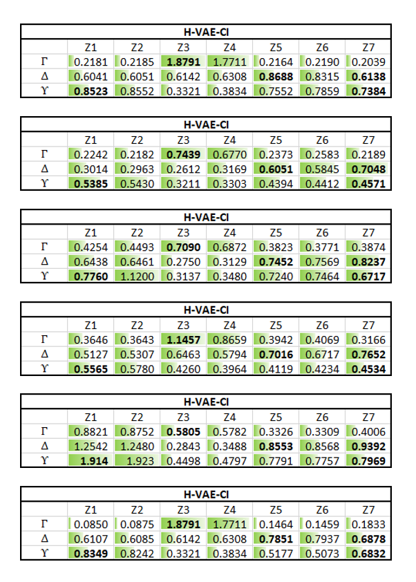
Figure 11: Decomposition tables for H-VAE-CI with $\beta\!=\!0$.

References

- Burgess et al. [2018] C. Burgess, I. Higgins, A. Pal, L. Matthey, N. Watters, G. Desjardins, and A. Lerchner. Understanding disentangling in -VAE. arXiv preprint:1804.03599, 2018.
- Chen et al. [2018] R. T. Chen, X. Li, R. B. Grosse, and D. K. Duvenaud. Isolating sources of disentanglement in variational autoencoders. In NeurIPS, 2018.
- Goodfellow et al. [2014] I. Goodfellow, J. Pouget-Abadie, M. Mirza, B. Xu, D. Warde-Farley, S. Ozair, A. Courville, and Y. Bengio. Generative adversarial nets. In NeurIPS, 2014.
- Gordon and Hernández-Lobato [2020] J. Gordon and J. M. Hernández-Lobato. Combining deep generative and discriminative models for bayesian semi-supervised learning. Pattern Recognition, 100, 2020.
- Gretton et al. [2012] A. Gretton, K. M. Borgwardt, M. J. Rasch, B. Schölkopf, and A. Smola. A kernel two-sample test. JMLR, 13(March), 2012.
- Guo et al. [2018] R. Guo, L. Cheng, J. Li, P. R. Hahn, and H. Liu. A survey of learning causality with data: Problems and methods. arXiv preprint:1809.09337, 2018.
- Harada and Kashima [2020] S. Harada and H. Kashima. Counterfactual propagation for semi-supervised individual treatment effect estimation. ECML-PKDD, 2020.
- Hassanpour and Greiner [2019] N. Hassanpour and R. Greiner. Counterfactual regression with importance sampling weights. In IJCAI, 2019.
- Hassanpour and Greiner [2020] N. Hassanpour and R. Greiner. Learning disentangled representations for counterfactual regression. In ICLR, 2020.
- Higgins et al. [2017] I. Higgins, L. Matthey, A. Pal, C. Burgess, X. Glorot, M. Botvinick, S. Mohamed, and A. Lerchner. -VAE: Learning basic visual concepts with a constrained variational framework. ICLR, 2017.
- Hill [2011] J. L. Hill. Bayesian nonparametric modeling for causal inference. Journal of Computational and Graphical Statistics, 20(1), 2011.
- Hoffman et al. [2017] M. Hoffman, C. Riquelme, and M. Johnson. The -VAE’s implicit prior. 2017. URL http://bayesiandeeplearning.org/2017/papers/66.pdf.
- Holland [1986] P. W. Holland. Statistics and causal inference. Journal of the American statistical Association, 81(396), 1986.
- Imbens and Rubin [2015] G. W. Imbens and D. B. Rubin. Causal Inference for Statistics, Social, and Biomedical Sciences: An Introduction. Cambridge University Press, 2015.
- Johansson et al. [2016] F. Johansson, U. Shalit, and D. Sontag. Learning representations for counterfactual inference. In ICML, 2016.
- Kingma and Ba [2015] D. P. Kingma and J. L. Ba. Adam: A method for stochastic optimization. In ICLR, 2015.
- Kingma and Welling [2014] D. P. Kingma and M. Welling. Auto-encoding variational bayes. In ICLR, 2014.
- Kingma et al. [2014] D. P. Kingma, S. Mohamed, D. J. Rezende, and M. Welling. Semi-supervised learning with deep generative models. In NeurIPS, 2014.
- Kuang et al. [2017] K. Kuang, P. Cui, B. Li, M. Jiang, S. Yang, and F. Wang. Treatment effect estimation with data-driven variable decomposition. In AAAI, 2017.
- Locatello et al. [2019] F. Locatello, S. Bauer, M. Lucic, G. Raetsch, S. Gelly, B. Schölkopf, and O. Bachem. Challenging common assumptions in the unsupervised learning of disentangled representations. In ICML, 2019.
- Lopez et al. [2018] R. Lopez, J. Regier, M. I. Jordan, and N. Yosef. Information constraints on auto-encoding variational bayes. In NeurIPS, 2018.
- Louizos et al. [2015] C. Louizos, K. Swersky, Y. Li, M. Welling, and R. Zemel. The variational fair autoencoder. arXiv preprint:1511.00830, 2015.
- Louizos et al. [2017] C. Louizos, U. Shalit, J. M. Mooij, D. Sontag, R. Zemel, and M. Welling. Causal effect inference with deep latent-variable models. In NeurIPS. 2017.
- MacDorman and Atkinson [1998] M. F. MacDorman and J. O. Atkinson. Infant mortality statistics from the 1996 period linked birth/infant death dataset. Monthly Vital Statistics Report, 46(12), 1998.
- Mansour et al. [2009] Y. Mansour, M. Mohri, and A. Rostamizadeh. Domain adaptation: Learning bounds and algorithms. arXiv preprint:0902.3430, 2009.
- McCallum et al. [2006] A. McCallum, C. Pal, G. Druck, and X. Wang. Multi-conditional learning: Generative/discriminative training for clustering and classification. In AAAI, 2006.
- Ng and Jordan [2002] A. Y. Ng and M. I. Jordan. On discriminative vs. generative classifiers: A comparison of logistic regression and naive bayes. In NeurIPS, 2002.
- Pearl [2009] J. Pearl. Causality. Cambridge University Press, 2009.
- Peters et al. [2017] J. Peters, D. Janzing, and B. Schölkopf. Elements of causal inference: foundations and learning algorithms. MIT press, 2017.
- Rezende et al. [2014] D. J. Rezende, S. Mohamed, and D. Wierstra. Stochastic backpropagation and approximate inference in deep generative models. ICML, 2014.
- Rosenbaum and Rubin [1983] P. R. Rosenbaum and D. B. Rubin. The central role of the propensity score in observational studies for causal effects. Biometrika, 1983.
- Rubin [1974] D. B. Rubin. Estimating causal effects of treatments in randomized and nonrandomized studies. Journal of Educational Psychology, 66(5), 1974.
- Shalit et al. [2017] U. Shalit, F. D. Johansson, and D. Sontag. Estimating individual treatment effect: Generalization bounds and algorithms. In ICML, 2017.
- Shi et al. [2019] C. Shi, D. Blei, and V. Veitch. Adapting neural networks for the estimation of treatment effects. In NeurIPS, 2019.
- Yao et al. [2018] L. Yao, S. Li, Y. Li, M. Huai, J. Gao, and A. Zhang. Representation learning for treatment effect estimation from observational data. In NeurIPS, 2018.
- Yoon et al. [2018] J. Yoon, J. Jordon, and M. van der Schaar. GANITE: Estimation of individualized treatment effects using generative adversarial nets. In ICLR, 2018.
- Zhang et al. [2021] W. Zhang, L. Liu, and J. Li. Treatment effect estimation with disentangled latent factors. In AAAI, 2021.