A new insight of AGC 198691 (Leoncino) galaxy with MEGARA at the GTC

Abstract

We describe the observations of the low-metallicity nearby galaxy AGC 198691 (Leoncino Dwarf) obtained with the Integral Field Unit of the instrument MEGARA at the Gran Telescopio Canarias. The observations cover the wavelength ranges 4304 – 5198 Å and 6098 – 7306 Å with a resolving power R $\approx$ 6000. We present 2D maps of the ionized gas, deriving the extension of the Hii region and gas kinematics from the observed emission lines. We have not found any evidence of recent gas infall or loss of metals by means of outflows. This result is supported by the closed-box model predictions, consistent with the oxygen abundance found by other authors in this galaxy and points towards Leoncino being a genuine XMD galaxy. We present for the first time spatially resolved spectroscopy allowing the detailed study of a star forming region. We use popstar $+$ cloudy models to simulate the emission-line spectrum. We find that the central emission line spectrum can be explained by a single young ionizing cluster with an age of $\approx$ 3.5 $\pm$ 0.5 Myr and a stellar mass of $\approx$ 2 $\times\,$10³ M_$\sun$. However, the radial profiles of [O iii] $\lambda$ 5007Å and the Balmer lines in emission demand photoionization by clusters of different ages between 3.5 and 6.5 Myr that might respond either to the evolution of a single cluster evolving along the cooling time of the nebula ($\approx$ 3 Myr at the metallicity of Leoncino, Z$\approx$ 0.0004) or to mass segregation of the cluster, being both scenarios consistent with the observed equivalent widths of the Balmer lines.

1 Introduction

The properties of eXtremely Metal-Deficient (XMD) galaxies, such as gas and stellar kinematics, and their relationship with the environment, along with the mechanisms in place that preserve their low abundance until today, have been a matter of scrutiny for the last few decades. Based on these properties, XMD galaxies have been proposed as the natural laboratories for testing the processes of chemical enrichment right after the primordial nucleosynthesis, in conditions similar to those of the early Universe.

Thus, nearby low metallicity galaxies are considered the local counterparts of the high-redshift primeval star-forming galaxies. This astrophysical subject has been boosted in the last five years due to new observational facilities and techniques pushing the limits of currently operating telescopes, both in the local universe and at intermediate redshift. The two main contributors to this progress have been recent large-scale surveys, such as the Sloan Digital Sky Survey, SDSS, (, 2005) and new but still scarce detailed spectroscopic observations with medium-large aperture ($\geq$ 6.5m) telescopes.

Local XMD galaxies have proven hard to find. Under the assumption that all normal galaxies follow the Luminosity (L) – Metallicity (Z) correlation, where the luminosity is usually measured from the B-band absolute magnitude, over the whole abundance range, the L – Z relationship would predict a low luminosity for the most metal-poor galaxies (Skillman, Kennicutt & Hodge, 1989), so XMD galaxies would be intrinsically weak, and therefore difficult to be detected, unless a burst of star formation boosted the luminosity producing a strong emission line spectra. For this reason, most of the searches of these galaxies have been focused on finding objects with episodes of star formation, selecting the candidates for their blue excess or for the high values of [O iii] $\lambda$ 5007/H_β, e.g., Izotov & Thuan (2007), Guseva et al. (2017), Hirschauer et al. (2018), Izotov et al. (2018a) and Izotov et al. (2019a). Moreover, [O iii] lines are the result of the ionization by a relatively hard spectrum only present in very young star clusters of age $\leq$ 5.5 Myr, as shown by García-Vargas, Bressan, Díaz (1995a, b) and later confirmed with the evolutionary synthesis models popstar (Mollá, García-Vargas, Bressan, 2009, hereafter M09).

Galaxy luminosity is strongly linked to recent star formation activity, and all the galaxies cataloged as XMD so far have been observed while experiencing a strong burst of star formation. The gas is ionized by a very young cluster, only a few Myr in age, making these XMD galaxies detectable in optical [OIII] lines. However, popstar models (M09) predict, for a single burst of star formation and a similar cluster’s mass and H${\alpha}$ luminosity, that the lower the metallicity the larger the age range in which the emission line spectrum can be detected, so the low abundance by itself cannot justify the detection difficulty. The origin behind the bias of XMD in mid-aperture telescope surveys seems to be a lower probability of capturing the episodes of star formation, due to an intrinsic low luminosity or/and a slow and quiet evolution.

A crucial point for XMD classification is the assignment of metallicity, usually done through the gas-phase oxygen abundance in the optical emission line spectrum of the ionized gas. The detailed description of how the oxygen abundance is obtained from observations in the optical range can be found in Osterbrock & Ferland (2006) and, more recently, in Pérez-Montero (2014). Briefly, the method consists in the determination of the average electron density, $n_{\rm e}$, of the gas from density-sensitive lines like [S ii] or [O ii], followed by the determination of the electronic temperature, T_e, of the ionized nebula. In particular, T_e ([O iii]) is obtained from the ratio $R_{\rm O3}$ = (I₄₉₅₉ + I₅₀₀₇) / I₄₃₆₃. The lines [O iii] $\lambda$ 4959, 5007 Å are very bright, especially in the low metallicity regions while the line [O iii] $\lambda$ 4363 Å is very weak, of the order of 1-2 % of the intensity of [O iii] $\lambda$ 5007. Thus, the measurement of the [O iii] $\lambda\,$4363 emission line is challenging, and imposes a bias in the low metallicity value depending on the telescope aperture, spatial resolution, spectroscopic field-of-view and affordable exposure times. When no detection of [O iii] $\lambda$ 4363 line is available, the oxygen abundance could be inferred from other emission lines. However, these methods have led to important discrepancies on the metallicity values (Andrews and Martini, 2013; Marino et al., 2013, and references therein) in the lowest range, which is the case for XMD galaxies.

The metallicity could also be estimated from diagnostic diagrams when different emission line ratios are used simultaneously. Martín-Manjón et al. (2010, hereafter M10) used Spectral Energy Distributions (SEDs) synthesis $+$ photoionization code cloudy to predict the emission line spectrum produced by an ionizing Single Stellar Population, SSP, under certain hypotheses on the Initial Mass Function, IMF, the chemical composition of the ionizing star clusters, Z, surrounding gas abundance and electron density, $n_{\rm e}$, and geometry (ionization bounded). They reached metallicities as low as Z $=$ 0.0004 (0.023 Z_$\sun$ equivalent to 12 + log (O/H) = 7.05) and Z $=$ 0.0001 (0.0058 Z_$\sun$, equivalent to 12 + log (O/H) =  6.45). M10 presented four diagnostic diagrams (see their figures 9, 10, 11 and 12) at different metallicities for the ionizing cluster and the surrounding gas. In particular, for values as low as those needed for reaching the lowest metallicity HII regions when plotting models, for a wide range of ionizing cluster ages and masses. This low-metallicity HII region locus in the diagnostic diagrams might be representative of XMD observations. The lowest metallicity models have intrinsic limitations, such as the uncertainty in both evolutionary tracks and atmosphere models of low metallicity stars and the cooling time in the ionized nebula. This cooling time is comparable to the age of the ionizing cluster itself, as computed and discuss in M10. Nevertheless, there are still very few observations for XMD with reliable metallicity and good values of all these lines to test the goodness of these diagrams as XMD abundance estimators.

A few years ago, a new technique based on selecting galaxies with low H i mass and bright optical emission line counterpart, has allowed the discoveries of few more XMD as Leoncino (Hirschauer et al., 2016, hereafter H16). However, these XMD galaxies studies are still based on emission line spectra, biased to the time when these galaxies are undergoing a burst of star formation. This in turn, biases the samples as most quiet low-metallicity old galaxies without recent star formation are missing, pointing towards these galaxies being not less numerous but less detectable as we need to go deeper in luminosity. Moreover, these galaxies would have low gas mass content and/or a low Star Formation Rate, SFR, at least for genuine XMDs, making the detection less likely.

The maximum oxygen abundance value to classify a galaxy as XMD differs among different authors and works (Kunth & Östlin, 2000; Izotov & Thuan, 2007; Izotov et al., 2012; Guseva et al., 2015; Sánchez-Almeida et al., 2016; Kojima et al., 2020) and, for years, was modulated by the value of the solar abundance itself. Just 20 years ago, the value of 12 + log(O/H)$\leq$ 7.65 was setup as the limit to be an XMD galaxy by Kunth & Östlin (2000). However, the number of the discoveries of XMD galaxies has increased so much in the last few years that the abundance of 12 + log(O/H) $\leq$ 7.35, equivalent to 0.046 Z_$\sun$, roughly a twentieth of the current value of the solar metallicity, is now considered to be the upper limit, see e.g. Guseva et al. (2017) and McQuinn et al. (2020, hereafter MQ20). Some authors even point to a value of 12 + log(O/H) $\leq$ 7.15, as minimum oxygen abundance to be XMD (H16). The competition for finding these objects is open and, until now, the lowest metallicity galaxies are J1631+4426 (Kojima et al., 2020), J0811+4730 (Izotov et al., 2018a), Leoncino galaxy (H16) and J1234+3901 (Izotov et al., 2019a), with 12 + log(O/H) equal to 6.90 $\pm$ 0.03, 6.98 $\pm$ 0.02, 7.02 $\pm$ 0.03, recently reported as 7.12 $\pm$ 0.04 (unpublished) by MQ20 and 7.035 $\pm$ 0.026, respectively.

There are other two fundamental aspects related to these galaxies. The first one is how the gas abundance is linked to the stellar metallicity of the galaxy while the second one is what is the origin of the low metallicity, being both associated to the history of star formation in the galaxy and the interaction with the surrounding gas. Assuming a sole old stellar population in the galaxy, its metallicity would map the gas metal content when stars formed, while the gas abundance would fit the current metallicity. However, the underlying stellar population is the combination of the different generations of stars created at different epochs tuned by the SFR of the galaxy and enriched according to its chemical evolution. For example, if the SFR was high in the past, we would expect to observe an enriched gas, so an explanation of the observed low metallicity would be the dilution by infall gas or the loss of metals by means of outflows. In contrast, if the star formation history was slow, due to an inefficient star formation or a small amount of gas available to fuel the star formation, the gas and old star population might have similar (low) metallicity. The latter scenario reinforces the scarcity of these XMD galaxies due to the low probability of capturing the star formation burst episode.

There have been many papers focused in disentangling the star and gas abundances in the XMD galaxies. One of the most used tools have been the relationship between the mass in stars, M_$\ast$, and the metallicity, Z (Berg et al., 2012; Guseva et al., 2017). The stellar mass has to be indirectly inferred by comparison of an observable, e.g. spectra or colours, with galaxy evolution models, each one with its own hypotheses and limitations, leading to different conclusions in terms of the dominant stellar populations in the galaxy and its total stellar mass. In the first published works on this topic, a universal M_$\ast$ – Z relation was put forward. However, with the advent of more observations and models, this relation became a matter of intense debate. On the one hand, for massive spiral galaxies (M_$\ast$ $\geq$ 10^10.5 M_$\sun$) the M_$\ast$ – Z relation starts to flatten (Tremonti et al., 2004; Hirschauer et al., 2018), while for XMD galaxies (M_$\ast$ $\leq$ 10⁹ M_$\sun$) large discrepancies were found resulting in significant disagreements among different works (Hirschauer et al., 2018, and references therein). Berg et al. (2012) obtained a strong correlation between M_$\ast$ and Z, with measured oxygen abundance higher for higher galaxy mass. They used observed values of the luminosity at 4.5 $\mu$m and the (B – K) colour and compared them with the values predicted by the models of Bruzual & Charlot (2003), assuming a Salpeter IMF and under the hypothesis that the 4.5 $\mu$m luminosity is mostly dominated by low-mass main-sequence and Red Giant Branch (RGB) stars. However, Guseva et al. (2017) presented a different M_$\ast$ – Z relation for XMD galaxies, finding a flatter relation of abundance when the stellar mass is derived from SEDs including nebular continuum emission, not present in the Bruzual & Charlot (2003) models Guseva et al. (2017) worked under the hypothesis that the star formation history of XMD galaxies can be represented by a short burst with age $\leq$ 10 Myr plus an old population formed in a rather continuous way. By fitting the model to their observations, they find values of the SFR between 0.1 and 1.0 M_$\odot$ yr^-1 and a specific SFR, defined as SFR/M_$\ast$, of about 50 Gyr^-1, similar to the one found by these same authors in previous works for star forming galaxies at redshifts 2 $<$ z $<\,$4.

Finally, the answer to the question on the origin of the lack of metals in XMD galaxies is also a matter of debate. Ekta & Chengalur (2010) summarized the following three possibilities: 1) a genuine low metallicity, 2) a dilution of the metals by pristine gas falling and 3) a preferential loss of metals.

The first scenario assumes that the low metal content is genuine, so that there is and always was a small amount of metals, implying that the galaxy has held a very low rate of star formation over a long period of time. This might occur if the galaxy is isolated enough, although there is some controversial in the interpretation of data supporting this argument (Kewley & Dopita, 2002). Alternatively, the cause can be a slow and different chemical evolution, lower than usual SFR over the galaxy age, inferring an inefficient triggering of star formation (Gavilán et al., 2013). Under this assumption, the low metal content of these galaxies has been studied to put an upper limit to the primordial helium abundance (Cyburt et al., 2016, and references therein), to constrain simulations of the formation of very low-mass galaxies and to test evolutionary models of massive stars out of pristine gas (Szécsi, 2016, and references therein).

The second scenario assumes a dilution of the metals by pristine gas falling into the galaxy from the outer disk, if existent, or from the local environment, like a consequence of an interaction with a neighbour galaxy. In the latter case, the infalling gas would trigger a quick mix of the galaxy material, producing a lower abundance (Ekta & Chengalur, 2010, MQ20). However, Dalcanton (2007) showed that for such galaxies, the effective yield tends asymptotically to a constant value independent of the gas mass, implying that the inflow of metal-poor gas cannot substantially lower the effective yield of extremely gas-rich galaxies. This mechanism, therefore, does not seem to be the one responsible of the low metallicity in very gas rich galaxies, as the XMD found in HI surveys.

The two scenarios described above are very different as they pointed to distinct causes of the low abundance. In the first one, the metals are not created in the XMD galaxy because the SFR is very low and, consequently, the mass created in new stars will be very low too. In the second scenario, metals are created and they are present in the gas, but an infall of primordial (or less enriched) gas would dilute the proportion of them in the total gas mass, with the corresponding abundance decrease. Gavilán et al. (2013) developed self-consistent chemical evolution and spectrophotometric models of the formation and evolution of gas-rich dwarf galaxies, with recent star formation but not bursting (i.e. dIrr), considering infall of primordial external gas but excluding outflow or galactic winds. They compare their predictions with observational data and conclude that such galaxies with moderate to low SFRs may be able to preserve the vast majority of their gas and metals.

The third scenario assumes that there was a more metallic content, but a significant part of these metals have been lost by violent phenomena, e.g. supernova (SN) events or outflows like enriched galactic winds. In the last years, this metal loss scenario has been the preferred one to explain the low abundance, as in the case of the LeoP galaxy, where, with an abundance of 12 + log(O/H) = 7.17 $\pm$  0.04 (Skillman et al., 2013, MQ20), it seems that 95 $\pm$ 2 per cent of its oxygen would have been lost through galactic winds (McQuinn et al., 2015a, b).

The XMD galaxies study demands to move to the next step: 2D spectroscopy in the optical range to derive, on the one hand, the age and metallicity of the stellar populations and, on the other hand, the gas metallicity and kinematics along the extension of the galaxy. To accomplish this goal, we need a large aperture telescope, to reach the low luminosity objects, with a spectral resolution high enough to decouple the emission line fluxes and kinematics of different physical components, and good spatial resolution to minimize the aperture effects and to place the different burst of star formation. These observations in the visible are more useful if the galaxies have HST high spatial resolution images or UV spectroscopy that unveil the young stellar clusters, hidden by the ionized gas in the ground-based optical spectra. Last but not least, the use of evolutionary synthesis and chemical evolution models is crucial to infer the physical properties of the stellar populations (mass, age and metallicity) and the star formation history.

MEGARA (Multi Espectrógrafo en GTC de Alta Resolución para Astronomía) offers all the required capabilities in the world largest optical telescope, the 10.4 m Gran Telescopio Canarias (GTC), at the Observatorio del Roque de los Muchachos located in La Palma, Spain. MEGARA observations allow us to derive maps of the gas properties at different galactocentric distances that can provide clues on the origin of the low metal content and the confinement (or not) of the ionized gas around the young clusters.

This paper is dedicated to present and discuss the results taken with MEGARA Integral Field Unit, IFU, on Leoncino galaxy. The spectra have resolving power of R $\approx$ 6000, in two different configurations corresponding to the spectral regions around H${\beta}$ and [O iii]$\lambda$ 5007, and H${\alpha}$, respectively. Section 2 summarizes the published results on Leoncino galaxy. Section 3 presents our observations, data reduction and analysis. The results are detailed in section 4 with the discussion in section 5, finishing with the conclusions in section 6.

2 Leoncino galaxy data from literature

The galaxy AGC 198691 (also known as the little lion and nicknamed Leoncino) was discovered and catalogued as the most metal-poor gas-rich galaxy known at the time (H16). This galaxy formed part of the the Arecibo Legacy Fast ALFA blind [H i] survey, ALFALFA (Giovanelli et al., 2005; Haynes et al., 2011; Giovanelli et al., 2013; Haynes et al., 2018), and has an estimated gas mass M${}_{\text{H\,{i}}}\,\leq 10^{7}$ M_☉. It was included for following up in the Survey of HI in Extremely Low-mass Dwarfs, SHIELD (Cannon et al., 2011) for ALFALFA galaxies with 10${}^{6}\,$M${}_{\odot}\,\leq$  M${}_{\text{H\,{i}}}\,\leq\,10^{7.2}$ M_⊙ and optical counterparts in the SDSS (, 2005). H16 obtained R-band and H${\alpha}$ images with the WIYN 0.9 m telescope and optical long-slit (1.2 $\times$ 10  arcsec²) spectroscopic data on the 4 m Mayall telescope at the Kitt Peak National Observatory (KPNO), under seeing conditions of 1.4 arcsec FWHM using the Kitt Peak Ohio State Multi-Object Spectrograph, KOSMOS, in both its blue and red arms with reciprocal dispersion of 0.66 and 0.99 Å pixel^-1, respectively. They also presented 0.8 arcsec seeing observations using the Blue Channel Spectrograph at the 6.5 m Multi Mirror Telescope (MMT) with slits of 1 and 1.5 arcsec in width and a linear dispersion of 1.19 Å pixel^-1. All observations were flux calibrated and taken along the parallactic angle. The extraction slit lengths were of 3.21 and 2.70 arcsec for the KPNO and the MMT observations, respectively. These authors reported a complete emission line analysis for that central spectrum with MMT composite data obtaining values of $T_{\rm e}$ = 19130 $\pm$ 800 K, $n_{\rm e}$ = 270 $\pm$ 200 cm^-3 and 12 + log(O/H) = 7.02 $\pm$ 0.03. They estimated a distance to the galaxy, obtained using the velocity flow model employed by the ALFALFA team, of 7.7 Mpc.

Recently, MQ20 published a comprehensive work on Leoncino imaging data obtained with HST. The galaxy was observed by the HST/WFC3-UVIS instrument (date: 2018-04-24, PID: 15243, PI: McQuinn) using the F606W and F814W UVIS2 filters for a total of 15018 and 18618 s, respectively. MQ20 presented a detailed photometric analysis using the dolphot package (Dolphin, 2000) and built a final single-star Colour – Magnitude Diagram, CMD, including 147 stars, with a mix of young and old populations composed by Red Super Giants (RSG), red HeB and Asympthotic Giant Branch (AGB) stars to which they assigned ages of 25, 50 and 100 Myr, respectively, using the parsec isochrones (Bressan et al., 2012). MQ20 derived a minimum mass for the cluster hosting RSG stars of 3 $\times$ 10⁵ M_$\sun$. On the other hand, based on the integrated flux at the 3.6 $\mu m$ IRAC band of ($1.50\pm 0.07$) $\times$ 10^-5 Jy (J. M. Cannon et al., in preparation) and assuming a mass-to-luminosity ratio of 0.47 (McGaugh & Schombert, 2014), they report a total stellar mass, M_$\ast$, of 7.3 ${}^{+2.2}_{-4.3}$ $\times$ 10⁵ M_$\sun$. Using the brightness of the Tip of the Red Giant Branch (TRGB) in their CMD as a distance indicator, MQ20 obtained a distance modulus of 30.40 ${}^{+0.31}_{-0.60}$ mag, which corresponds to a distance of 12.1 ${}^{+1.7}_{-3.4}$ Mpc. This value places Leoncino in an under-dense galaxy environment at the position of void number 12 of the Pustilnik catalogue (Pustilnik, Tepliakova & Makarov, 2019). Likewise, using the TRGB method on single-star photometry with HST data Tikhonov & Galazutdinova (2019) calculated the distances to 18 dwarf galaxies from the Arecibo survey, including Leoncino, which was found to be located at 8.8 Mpc, marginally consistent, with the MQ20 determinations.

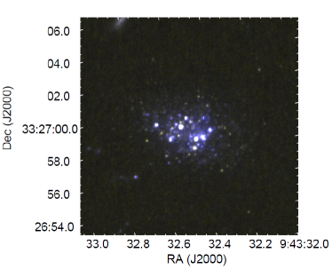
Figure 1: Image of the galaxy Leoncino based on HST/WFC3-UVIS data. The F606W image is used as blue channel while the F814W image is used for both the green and red channels. The plate scale of these HST images is 0.04 arcsec pixel^-1. This image shows a region of $14\,\times 14$  arcsec² around the target coordinates, slightly larger than the field-of-view covered by our MEGARA observations, $12.5\,\times\,11.3$  arcsec².

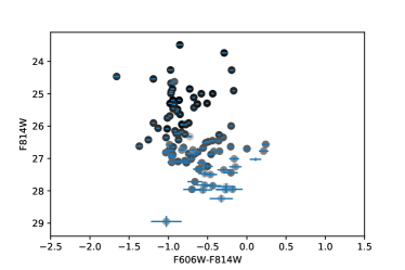
Figure 2: CMD of a region of 6 arcsec (150 pixels) in radius around the central coordinates of the galaxy. The figure shows, color-coded, the sources detected as a function of the distance to the galaxy center (as derived by MQ20 from HST images), darker shades indicate smaller galactocentric distances. The stars with values of F814W lower than 26.5 mag are basically outside the central 2 arcsec (50 pixels). The magnitudes are given in STMAG system.

Fig. 1 shows an image of the galaxy that we obtained from HST archive using the F606W image as blue channel and the F814W image for both the green and red channels. This image shows a region of $14\times 14$ arcsec² around the target center coordinates, $\alpha~{}$(J2000.0 FK5) =  09^h 43^m 32.40^s and $\delta~{}$(J2000.0 FK5) = $+33^{\circ}26^{\prime}57.9^{\prime\prime}$, with a plate scale of 0.04 arcsec pixel^-1. We had re-done the single-star photometry analysis using the drizzle images available through MAST and running the daofind and phot iraf tasks to obtain V (F606W) and I (F814W) magnitudes for all sources detected above 5$\sigma$ (4$\sigma$) in the combined F606W (F814W) image. Fig. 2 shows the resulting CMD of a 6 arcsec (150 pixels) radius region around the center of the galaxy (we have taken the one derived by MQ20 from HST images). The diagram shows in gray-scale the sources detected as a function of the distance to the galaxy center, where points of darker shade correspond to stars placed closer to the galaxy center. The stars with values of F814W lower than 26.5 mag are basically outside the central 2 arcsec (50 pixels). The magnitudes are given in STMAG system. A bright and blue main-sequence is clearly visible along with some RSG stars. Outside the central 2 arcsec, equivalent to 110 pc at the distance derived by MQ20, less massive red stars are detected. This could be indicative of the presence of an intermediate-aged stellar population in the outskirts of this system. These results are fully in agreement with the ones derived by MQ20.

Leoncino is located at a projected distance of 46 kpc from UGC 5186 galaxy, and with an offset of only 35 km s^-1, which led MQ20 to suggest a possible interaction between both galaxies, further supported by the detection of H i between them. Based on this fact and the positioning of Leoncino in the M – Z relation, they proposed that Leoncino has been experimenting an inefficient star formation history overall, dominated by individual episodic bursts whose associated galactic winds would be the cause of its low metal abundance. The most recent star formation bursts would have been triggered as the result of a minor interaction with its neighbor UGC 5186. Regarding its gas mass content, at the distance determined by MQ20, M${}_{\text{H\,{i}}}$ results in $1.83\times 10^{7}$ M_$\sun$. As mentioned, these authors report a value of 12 + log(O/H) = 7.12 $\pm\,$0.04 from an observation with the Large Binocular Telescope (LBT). Recently, Aver et al. (2021) revised this value to 12 + log(O/H) = 7.06 $\pm\,$0.03, obtained from the same LBT observation.

We used the results from MQ20 for the gas mass of $1.83\times 10^{7}$ M_$\sun$ and stellar mass ranging between 6.5 and 7.3 $\times\,10^{5}$ M_$\sun$ to calculate the predicted oxygen mass abundance, Z_O, in a closed-box chemical evolutionary model. Z_O is determined through the equation Z_O = p${}_{\rm O}\times\ln{\mu}^{-1}$, where p_O is the oxygen integrated yield and $\mu$ is the ratio between the gas and the total (stellar and gas) mass. By using the integrated stellar yields from Mollá et al. (2015), we obtain a value of Z_O between 2.3 $\times 10^{-5}$ and 8.4 $\times 10^{-4}$, which would correspond to 12  $+$  log(O/H) between 6.28 and 7.85 depending on the combination IMF + stellar yields used for the integrated yield, p_O. The average predicted oxygen abundance using the whole set of 144 integrated yields from Mollá et al. (2015) is 12 + log(O/H) $=$ 7.17, which corresponds to the mode of the distribution obtained for all of them, being 6.28 and 7.85 the minimum and the maximum, respectively. Therefore, any oxygen abundance between the two is possible, with a higher probability in the range between 6.80 and 7.40, and being the most likely value 7.17 (7.15 when using the IMF of Kroupa (Kroupa, 2001) and Z = 0.0004, for which the integrated yield varies between 0.001 and 0.007), close to the reported abundances. These closed-box model results are consistent with a genuine low metallicity in Leoncino.

3 MEGARA observations and data analysis

We present and discuss IFU observations of Leoncino galaxy obtained with MEGARA at GTC. MEGARA is an optical (3650 – 9750 Å) fiber-fed spectrograph. The instrument offers two modes: integral-field and multi-object spectroscopy. The IFU provides a field of view (FoV) of 12.5 $\times$ 11.3 arcsec², plus eight additional mini-bundles, located at the edge of the FoV, for simultaneous sky subtraction. The spatial sampling is 0.62 arcsec per fiber, thanks to the combination of a 100 $\upmu$m core fibre coupled to a microlens that converts the f/17 entrance telescope beam to f/3, to minimize the fibers focal ratio degration and to maximize the efficiency. The spaxel projection is over-sized relative to the fiber core for a precise fiber-to-fiber flux uniformity. A fiber link 44.5 m in length drives the light, coming from the folded Cassegrain focal plane into the spectrograph, which is placed at the GTC Nasmyth A platform. The spectrograph includes a set of 18 Volume Phase Holographic (VPH) gratings, offering three spectral modes with resolving power of R_FWHM $\approx$ 6 000, 12 000 and 20 000, for low, medium and high resolution, respectively. The scientific data are recorded by a deep-depleted Teledyne-e2V 4096 pix $\times$ 4096 pix detector with 15 $\upmu$m-pixel pitch. The instrument design and final performance on the GTC based on commissioning results can be found in Carrasco et al. (2018), Gil de Paz et al. (2018), and Gil de Paz et al. (2021, submitted).

3.1 Observations and Data Reduction

We observed Leoncino using as target coordinates $\alpha~{}$(J2000.0 FK5) =  09^h 43^m 32.36^s and $\delta~{}$(J2000.0 FK5) = $+33^{\circ}26^{\prime}57.6^{\prime\prime}$. The data were taken in the dark, clear night of February 2^nd 2019. We used the spectrograph configurations given by the VPH gratings labelled as LR-B and LR-R. LR-B ranges from 4304 to 5198 Å  with a reciprocal linear dispersion $\delta\lambda=0.23$ Å pixel^-1 and a FWHM spectral resolution element $\Delta\lambda=0.92$ Å, while the LR-R setup covers the interval from 6098 to 7306 Å  with $\delta\lambda=0.32$ Å  pixel^-1 and $\Delta\lambda=1.24$ Å. The average seeing was 0.8 arcsec and 0.6 arcsec for the LR-B and LR-R observations, respectively. Six 1200 s images (7200 s) and three 900 s exposures (2700 s) were taken with the LR-B and LR-R setups, respectively.

The observations had their associated calibrations: bias, halogen, ThAr (for LR-B) and ThNe (for LR-R) lamps, obtained for bias subtraction and modelling, tracing and flatfielding, and wavelength calibration, respectively. These auxiliary images were obtained in daytime and in each case three identical exposures were done to facilitate the cosmic ray removal. Observations of the spectrophotometric standard star HR3454 were made to generate the response function for absolute flux calibration. The data were reduced with the MEGARA Data Reduction Pipeline, DRP, a python based software tool operating in command-line (Cardiel & Pascual, 2018; Pascual et al., 2018).

The resulting product of the DRP is a Row Stacked Spectra (RSS) FITS file, which contains the individual flux-calibrated spectra for all 623 fibers in the IFU. The MEGARA DRP also produces a final RSS image in which the sky has been subtracted by combining the signal of the seven (or a subsample of them) sky mini-bundles placed along the IFU pseudo-slit. We applied this standard sky-subtraction procedure for the LR-B data. The Quick Look Analysis (qla tool), developed by Gómez-Alvarez et al. (2018), allows the user to choose the sky bundles, optimizing the spectra extraction and visualization. We followed this sky-subtraction method to obtain the LR-R final RSS combined image. Additionally, we used the qla package to obtain reconstructed 2D images in specific spectral windows from the RSS spectra.

From the comparison of the HST and MEGARA coordinates of the clusters, we derived the shift between the two images and updated the headers of the MEGARA synthetic images to match the reference coordinates and orientation of the LR-R-based and HST reference images. A final minor astrometric correction was performed.

To ensure a correct absolute astrometry, the availability of HST imaging was crucial as there were no stars within the field of MEGARA IFU. The main sources of information come from the LR-R continuum image, where two knots can be detected matching the position of the brightest continuum sources in the HST F606W image, and the H$\alpha$ and H$\beta$ flux images. First, we aligned our LR-R continuum image with a precision that we estimate to be below half a spaxel ($\sim$0.3 arcsec). This automatically corrected the H$\alpha$ flux data as they come from the same spectral setup as our 6590 – 7100 Å continuum image. We then aligned the H$\beta$ flux image to the H$\alpha$ one (the low dust reddening ensures that potential offsets due to differential extinction should be negligible at these scales). This relative alignment is needed since the noise in the LR-B continuum reconstructed image is too high and no HST image bluer than F606W is available. The two setups turned out to be offset by 1.35 arcsec in right ascension and 0.35 arcsec in declination. So that the coordinates (J2000.0 FK5) for the center of MEGARA images are: $\alpha~{}$ =  09^h 43^m 32.40^s; $\delta~{}$ = +33${}^{\circ}26^{\prime}57.56^{\prime\prime}$. The centers of the brightest spaxels in the Balmer lines in LR-B and LR-R are $\alpha~{}$ =  09^h 43^m 32.59^s; $\delta~{}$ = $+33^{\circ}26^{\prime}55.89^{\prime\prime}$ and $\alpha~{}$ =  09^h 43^m 32.62^s; $\delta~{}$ = $+33^{\circ}26^{\prime}55.49^{\prime\prime}$ respectively, coincident at the level of half a spaxel and coherent within the seeing values.

We remark that the continuum emission level derived from the analysis of the LR-R data is of the order of 10^-6  Jy spaxel^-1, which matches the $\sim$ 4$\times 10^{-6}$ Jy arcsec^-2 surface brightness level in the HST image (0.05 electrons s^-1 pixel^-1) for that same region, given that the MEGARA IFU spaxel size is 0.25  arcsec². Here, we have obtained the conversion from electrons s^-1 to Jy in the HST data using the PHOTFNU keyword from the F606W image.

The corresponding astrometry correction was applied to all the results in this paper involving absolute positions (e.g. maps or comparison of the MEGARA-IFU and HST morphologies).

4 RESULTS

We produced several 2D maps throughout the galaxy. The description of the maps and the gas kinematics are presented in subsections 4.1 and 4.2, respectively. We performed extractions at different apertures, i.e. in an accumulative way, to show how the emission line fluxes and lines ratios change due aperture effects, as described in subsection 4.3. To analyze the emission line spectrum in different ionization rings we carried out a spaxel-to-spaxel extraction, using the qla package and the results are presented in subsection 4.4

In all the spectra we measured both, the line fluxes and their errors, using three different analysis packages: figaro, qla tool and the utility analyzed-spectrum of megaratools (Gil de Paz, Pascual & Chamorro-Cazorla, 2018). The three utilities produced the same values of the emission lines within the given errors. In case of discrepancy, we always used the largest error bar. The lines detected and measured wherever possible were in the LR-B spectra: H${\gamma}$, [O iii]$\lambda$ 4363Å (hereafter [O iii]4363), He i $\lambda$ 4471Å (hereafter He i 4471), H${\beta}$, [O iii]$\lambda$ 4959Å (hereafter [O iii] 4959), [O iii]$\lambda$ 5007Å (hereafter [O iii] 5007) and He i $\lambda$ 5015Å (hereafter He i  5015). In the LR-R spectra: H${\alpha}$, [N ii]$\lambda$ 6584Å (hereafter [N ii] 6584), He i$\,\lambda$ 6678Å (hereafter He i 6678), [S ii]$\lambda$ 6717Å (hereafter [S ii 6717), [S ii]$\lambda$ 6731Å (hereafter [S ii]$\lambda$ 6731), He i $\lambda$ 7065Å (hereafter He i 7065), [Ar iii]$\lambda$ 7135Å (hereafter [Ar iii] 7135) and He i $\lambda$ 7281Å (hereafter He i 7281).

For the brightest lines in each setup, i.e. H${\beta}$, [O iii] 4959 and [O iii] 5007 in LR-B and H${\alpha}$, [N ii] 6584, [S ii] 6717 and [S ii] 6731 in LR-R, we systematically measured the emission-line properties including only spaxels with signal-to-noise per pixel (at the peak of the line) S/N $\geq$ 5. The emission-line properties, flux, recession velocity and velocity dispersion correspond to the zeroth, first, and second momenta of the best-fitting Gauss-Hermite line profile decomposition used by the analyzed-rss utility of megaratools (Gil de Paz, Pascual & Chamorro-Cazorla, 2018).

For our analysis, we have considered a distance to Leoncino of 7.7 Mpc (H16). This gives a scale of 22 pc spaxel^-1 and 37 pc arcsec^-1, consistent with the radial velocity of our own emission line spectrum and similar to other published results. The implications of considering other values of the distance are explained in 5.1. In particular, the spatial resolution given by the spaxel size would change from the value we assume of 22 pc for a distance of 7.7 Mpc to 42 pc for a 13.8 Mpc distance. In the tables and figures of this section, the observed projected distances are indicated in arcsec to facilitate a reference for scale conversion if using a different distance to Leoncino.

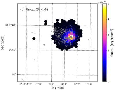
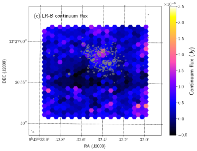
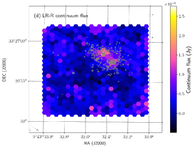
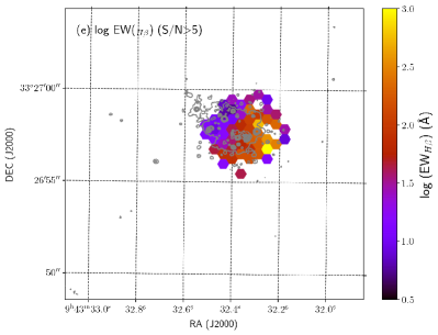
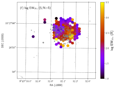
Figure 3: Top panels: emission line flux maps. Middle panels: maps (in Jy) for the H${\beta}$ continuum averaged between 4400 and 4850 Å (left) and for the H${\alpha}$ continuum averaged between 6590 and 7100 Å (right). Bottom panels: logarithm of the EW (in Å) of H${\beta}$ (left) and H${\alpha}$ (right). The actual FoV of the entire MEGARA IFU can be seen outlined in the continuum plots. In all cases the contours come from the HST archival image obtained with the WFC3-UVIS/HST instrument in the F606W band and correspond to 0.02, 0.07, 0.12, 0.17, 0.22, 0.27, 0.32 and 0.37 electrons s^-1 or 0.23, 0.8, 1.4, 1.9, 2.5, 3.1, 3.6 and 4.2 $\times$ 10^-20 erg s^-1 cm^-2 Å^-1.

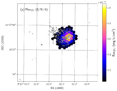
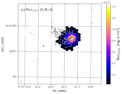
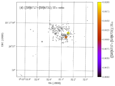
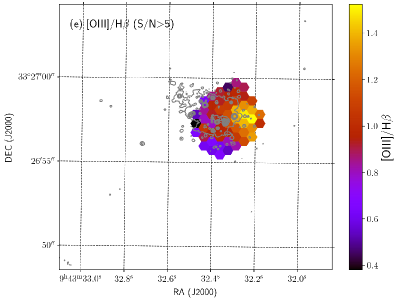
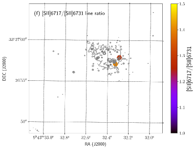
Figure 4: Left: maps of H${\beta}$ flux (top) and [O iii] 5007 (middle) flux (in erg s^-1 cm^-2) and [O iii] 5007/H${\beta}$ (bottom). Right: map of H${\alpha}$ flux (in erg s^-1 cm^-2) (top) and [S ii] 6717+6731/H${\alpha}$ (middle) and [S ii] 6717/[S ii] 6731 (bottom). In all cases the contours come from the HST archival image obtained with the WFC3-UVIS/HST instrument in the F606W band and correspond to 0.02, 0.07, 0.12, 0.17, 0.22, 0.27, 0.32 and 0.37 electrons s^-1 or 0.23, 0.8, 1.4, 1.9, 2.5, 3.1, 3.6 and 4.2 $\times$ 10^-20 erg s^-1 cm^-2 Å^-1.

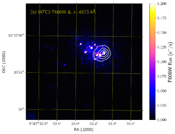
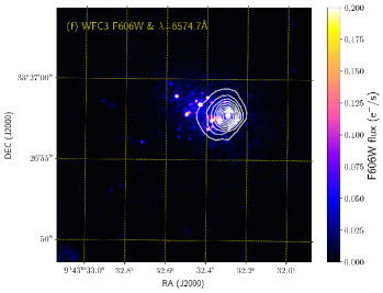
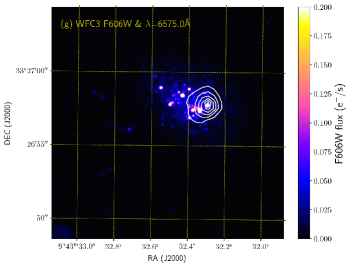
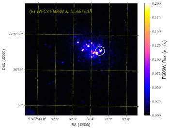
Figure 5: WFC3-UVIS/HST F606W image on which we have overlapped the velocity channels around H${\alpha}$ line, as described in subsection 4.2.

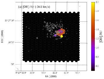
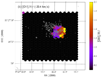
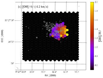
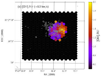
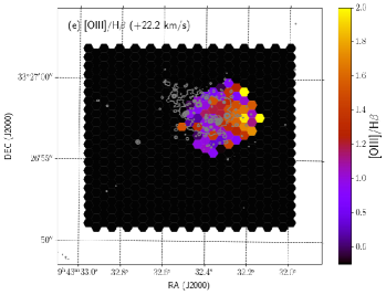
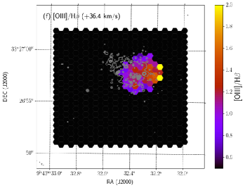
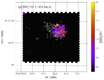
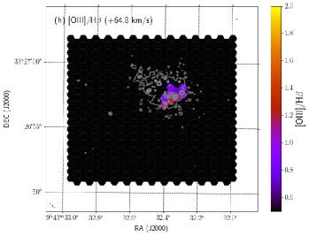
Figure 6: [OIII]/H$\beta$ ratio for different velocity channels. See description in subsection 4.2.

4.1 Emission line 2D maps

In Fig. 3 we show the results for the case of the H$\beta$ (left) and H$\alpha$ (right) lines from LR-B and LR-R data, respectively. The top panels show the emission line flux maps. The central panels, where proper size of the MEGARA IFU can be seen, display the continuum maps (in Jy) of H${\beta}$ (left), averaged between 4400 and 4850 Å and H${\alpha}$ (right), averaged between 6590 and 7100 Å. The bottom panels show the map of the logarithm of the equivalent width, EW, (in Å) for H${\beta}$ (left) and H${\alpha}$ (right), respectively. The contours come from the WFC3-UVIS F606W HST image and correspond to 0.02, 0.07, 0.12, 0.17, 0.22, 0.27, 0.32 and 0.37 electrons s^-1 or 0.23, 0.8, 1.4, 1.9, 2.5, 3.1, 3.6 and 4.2 $\times$$\times$ 10^-20 erg s^-1 cm^-2 Å^-1.

The H${\beta}$ and H${\alpha}$ line-flux maps in Fig. 3 show that the peak of line emission is associated to the westernmost blue stellar cluster detected in the HST data, see also the HST image shown in Fig. 1. In terms of physical extension we detect H$\alpha$ emission with S/N $>$ 5 reaching as far as $\sim$ 4 arcsec from this peak emission ($\sim$150 pc away from it). Besides, it is also worth noting that the region is slightly asymmetric, being more extended towards the NE than to the SW of the line-emission peak. This is discussed in greater depth in section 5 but given the distribution of the continuum in the F606W HST image this could be due either to photoionization by photons coming from other clusters located NE of the brightest cluster or to a change in the bounding regime in both directions: radiation bounded to the NE and density bounded instead in the SW direction. The same behavior is observed in the H$\beta$ flux map. Regarding the distribution in EW showed in the bottom panels of Fig. 3, we note that a negative gradient from the SW, where the line-emission peak is located, towards the NE of the galaxy. In addition, the close inspection of the region around this peak shows that the highest EW ($>$1000 Å) is reached not at the position of the spaxel with the brightest line emission but in the two spaxels located immediately SW from it, which suggests a spatial segregation between the ionized gas and the ionizing stars in spatial scales of a few tens of parsecs.

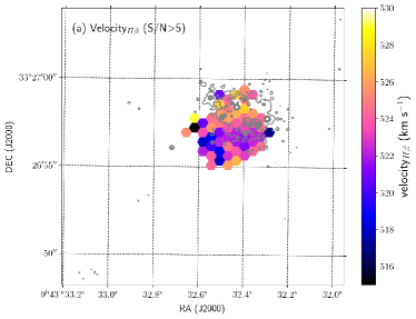
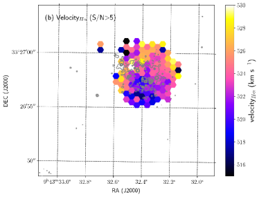
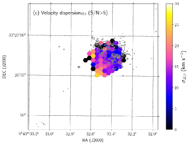
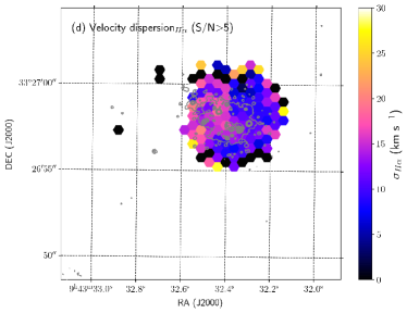
Figure 7: Maps of radial topocentric velocity (top) and velocity dispersion ${\sigma}$ (bottom), corrected from instrumental contribution, derived from the positions and widths of the H${\beta}$ (left) and H${\alpha}$ (right) lines. All values are in km s^-1.

We present in Fig. 4 some emission lines fluxes and flux ratio maps for the spaxels in which we have measured S/N $>$ 5 in every line involved. The left panels present the maps obtained from the LR-B image: flux (in erg s^-1cm^-2) of H${\beta}$ (top) and [O iii] 5007 (middle) and the ratio [O iii] 5007/H$\beta$ (bottom). The right panels display the maps from LR-R: flux (in erg s${}^{-1}\,$cm^-2) in H$\alpha$ (top), [S ii] 6717+6731/H${\alpha}$ (middle) and the ratio [S ii] 6717/[S ii]6731 (bottom). Fluxes with S/N $>$ 5 were measured in the [S ii] 6717, 6731 doublet for only two bright central spaxels. The contours are the same as in Fig. 3. Note that in this figure we include the same H$\beta$ and H$\alpha$ line-flux maps already shown in Fig. 3 for convenience when discussing our results below.

While the spatial distribution of the [O iii] 5007 line emission resembles closely that seen in H$\beta$, the line ratio map (bottom-left panel) shows significant radial and azimuthal variations, with the maximum being found W of the line-flux peak. We further discuss on the radial variation of the [O iii] 5007/H$\beta$ line ratio in section 5.2. In the middle and bottom-right panels we show the properties of the [S ii] 6717, 6731 doublet emission. Unfortunately, its emission is only detected in two of the spaxels, although they yield [S ii]/H${\alpha}$ line ratios of the order of 0.015-0.020.

4.2 Gas kinematics

Table 1: LR-B emission lines measurements in apertures around the central brightest spaxel. Fluxes are given in units of $\times$ 10^-17 erg cm^-2 s^-1 and EW in Å.

(1)	(2)	(3)	(4)	(5)	(6)	(7)	(8)	(9)	(10)	(11)	(12)	(13)
d	d	nr	Ns	H${\beta}$	H${\beta}$	H${\gamma}$	H${\gamma}$	[O iii]4363	[O iii]4959	[O iii]5007	He i4471	He i5015
pc	´´			Flux	EW	Flux	EW	Flux	Flux	Flux	Flux	Flux
11	0.31	0	1	10.50$\pm$1.03	213$\pm$168	5.09$\pm$1.45	44$\pm$43	0.38$\pm$0.44	5.18$\pm$0.73	14.42$\pm$1.06	0.26$\pm$0.26	0.20$\pm$0.17
33	0.93	1	7	57.71$\pm$2.64	306$\pm$136	28.53$\pm$3.86	24$\pm$8	1.93$\pm$1.10	26.51$\pm$2.22	74.19$\pm$3.19	2.78$\pm$0.80	1.07$\pm$0.47
55	1.55	2	19	104.60$\pm$4.19	177$\pm$52	55.05$\pm$6.78	18$\pm$5	4.08$\pm$2.23	44.92$\pm$2.74	126.30$\pm$4.05	4.26$\pm$1.43	1.41$\pm$0.70
77	2.17	3	37	134.70$\pm$5.15	101$\pm$21	77.44$\pm$8.71	13$\pm$3	5.44$\pm$3.14	56.40$\pm$3.33	155.70$\pm$4.88	4.71$\pm$1.82	2.53$\pm$0.98
121	3.41	All	63	160.70$\pm$6.40	76$\pm$15	96.27$\pm$11.44	9$\pm$2	7.71$\pm$4.74	62.86$\pm$3.99	171.90$\pm$6.01	6.32$\pm$2.75	2.73$\pm$1.43

Table 2: LR-R emission lines measurements in apertures around the central brightest spaxel. Fluxes are given in units of $\times$ 10^-17 erg cm^-2 s^-1 and EW in Å.

(1)	(2)	(3)	(4)	(5)	(6)	(7)	(8)	(9)	(10)	(11)	(12)	(13)
d	d	nr	Ns	H${\alpha}$	H${\alpha}$	[N ii]6584	He i6678	[S ii]6717	[S ii]6731	He i7065	[Ar iii]7135	He i7281
pc	´´			Flux	EW	Flux	Flux	Flux	Flux	Flux	Flux	Flux
11	0.31	0	1	58.67$\pm$1.89	1407$\pm$847	0.40$\pm$0.21	0.43$\pm$0.18	0.73$\pm$0.27	0.53$\pm$0.20	0.50$\pm$0.18	0.27$\pm$0.21	0.07$\pm$0.10
33	0.93	1	7	252.60$\pm$3.36	543$\pm$84	1.92$\pm$0.56	1.84$\pm$0.48	2.84$\pm$0.53	1.79$\pm$0.44	1.97$\pm$0.56	1.46$\pm$0.58	0.36$\pm$0.38
55	1.55	2	19	398.70$\pm$5.03	346$\pm$40	2.59$\pm$0.86	2.80$\pm$0.75	5.02$\pm$0.84	2.44$\pm$0.74	2.93$\pm$0.85	2.39$\pm$1.05	1.05$\pm$0.74
77	2.17	3	37	489.00$\pm$8.30	259$\pm$35	3.17$\pm$1.24	3.59$\pm$0.94	6.42$\pm$1.24	3.36$\pm$1.12	2.84$\pm$1.13	3.82$\pm$1.44	1.01$\pm$1.05
121	3.41	All	61	545.10$\pm$11.85	202 $\pm$31	4.09$\pm$1.78	4.17$\pm$1.45	7.72$\pm$1.91	2.41$\pm$1.44	2.68$\pm$1.41	3.59$\pm$2.01	1.66$\pm$1.42

In Fig. 5 we show the WFC3-UVIS/HST F606W image and overlapped are the velocity channels around the H${\alpha}$ line: the intensity contours correspond to 0.25, 0.50, 0.75, 1.00, 1.25, 1.50, 1.75, 2.00, 2.25, 2.50, 2.75, 3.00, 3.25, 3.50, 3.75, 4.00, 4.25, 4.50 and 4.75 $\times$ 10^-4 Jy. Note that the brightest contours are missing in some channels as these are tracing the wings of the H$\alpha$ line. In fact, only the 0.25 $\times$  10^-4 Jy contour is depicted in all 8 panels. This figure shows that there is little velocity structure within the region showing ionized-gas emission in the galaxy, since the peak of emission at different wavelengths is centered in the same region for all velocity channels. This indicates that either all the emission comes from a region with a common bulk motion or any rotational motion is mainly taking place in the plane of the sky. Besides, the mild asymmetry in the H$\alpha$ flux is also seen in the velocity channel maps for a wide range of velocities ($\pm$ 40 km s^-1 around its systemic velocity).

As mentioned in subsection 4.1 we find radial and azimuthal anisotropies in the [O iii] 5007/H$\beta$ ratio. One interpretation is the presence of a hot gas component flowing out through an opening in the giant Hii region (Menacho et al., 2019). Interestingly, this region of high excitation is located in the region where the H$\alpha$ surface brightness drops fastest. Such a drop could be due to the presence of density-bounded conditions in the SW of the galaxy, which would indeed favor the escape of hot gas from inside the nebula. To provide further clues to this possible scenario we have followed the methodology described by Menacho et al. (2019) for MUSE data but using our higher spectral resolution MEGARA-IFU data. In Fig. 6 we show the [O iii] 5007/H$\beta$ maps measured for each velocity channel in the range $-$34.6 to $+$64.8 km s^-1 around each of the lines with the F606W HST contours overlapped (0.02, 0.07, 0.12, 0.17, 0.22, 0.27, 0.32 and 0.37 electrons s^-1 or 0.23, 0.8, 1.4, 1.9, 2.5, 3.1, 3.6 and 4.2 $\times$ 10^-20 erg s^-1 cm^-2 Å^-1). Again, the high excitation gas is present at all velocities, i.e. both at the core and the wings of the emission lines, and the overall spatial variation of the [O iii] 5007/H$\beta$ ratio is also rather similar. This result indicate that either there is no high excitation gas flowing out of the region or its motion is taking place in the plane of the sky.

Additionally, in Fig. 7 we show the maps of topocentric radial velocity and velocity dispersion (in km s^-1) corrected from instrumental contribution, obtained from the analysis of the H${\beta}$ (left) and H$\alpha$ (right). While the velocity channels (Fig. 5) do not show a clear rotation pattern, when we map the velocities of the best-fitting Gauss-Hermite line profile in the case of the brightest H$\alpha$ line, we infer a mild velocity gradient with a projected maximum velocity of $\pm$ 5 km s^-1 assuming that the dynamical center is near the center of the region where radial velocities can be measured, as shown in the top panels.

Adopting this rotational velocity and a spherically symmetric mass distribution, the total enclosed mass at a galactocentric distance of 110 pc (3 arcsec) would be $6.4\times 10^{5}$ M_$\sun$. Note that although the assumption of spherical symmetry could yield this value as an upper limit (thin axisymmetric mass distributions generate the same radial force with a somewhat smaller enclosed mass), the fact that we have used the projected rotational velocity as the galaxy circular velocity, probably results in an underestimation of the true enclosed mass. The velocity dispersion measurements obtained are rather small, with values that, once corrected for instrumental dispersion, are as low as 10-15 km s^-1, even being compatible with zero in a few of the spaxels analyzed. We also find that the velocity dispersion values are slightly smaller in the E side of the nebula than in the W side of it, where the emission peak and the highest equivalent widths are found.

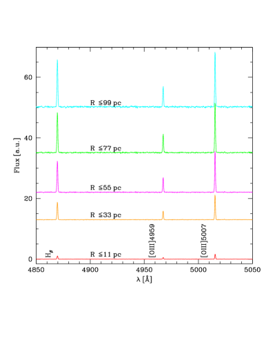
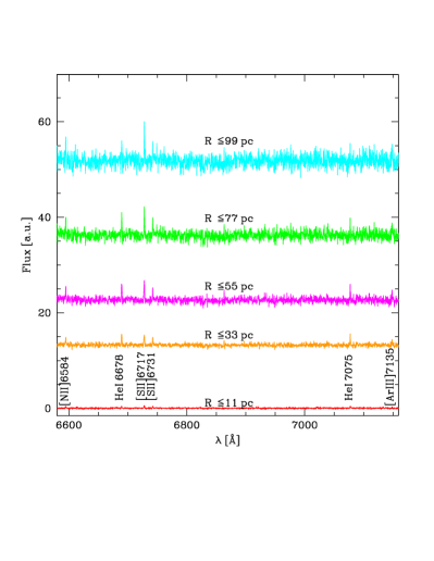
Figure 8: Accumulated spectra for LR-B (left) and LR-R (right) setups for increasing areas located at different distances of the center as labelled. Each spectrum is shifted an arbitrary distance for the sake of clarity.

Figure 9: Left: total flux accumulated in successive circular apertures around the most brightest spaxel, with respect to the flux in the central spaxel, for H${\alpha}$, H${\beta}$ and [O iii] 5007. Each of the apertures includes the inner ones. Right: ratio [O iii] 5007/H${\beta}$ as a function of the aperture.

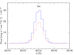
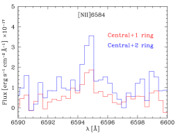
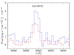
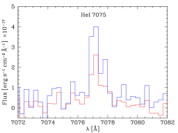
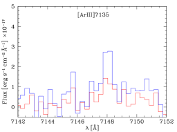
Figure 10: Accumulated spectra for the LR-R setup for two areas: one with the central ring and the first ring and the other adding contributions of the central ring and two rings, as labelled, for the spectral ranges where [N ii] 6584, He i 6678, [S ii] 6717, [S ii] 6731, He i 7065 and [Ar iii] 7135 emission lines are located.

4.3 Aperture effect in the emission line regions and the ionizing photon budget

We measured the emission lines in the spectra extracted using different circular apertures that would be equivalent to different slit widths. The corresponding spectra are shown in Fig. 8. In this case each spectrum includes the ones from the inner apertures, thus, the last one correspond to the integrated spectra of the global region of 140 pc. The measurements of the emission lines are shown in Table 1 and Table 2, for the LR-B and LR-R spectra, respectively. The first four columns in both are: (1) the distance from the central brightest spaxel to the limit of the extraction aperture, (2) the corresponding distance in arcsec, (3) the most external ionized ring included in the aperture being 0 the central spaxel and considering 22 pc between two consecutive rings and (4) the number of spaxels added in the spectrum for that aperture. Columns  5, 7, 9, 10, 11, 12 and 13 of Table 1 are the observed absolute fluxes, in units of $\times$ 10^-17 erg cm^-2 s^-1, of H${\beta}$, H${\gamma}$, [O iii] 4363, [O iii] 4959, [O iii] 5007, He i 4471 and He i 5015, respectively. Columns 6 and 8 give the EW of H${\beta}$ and H${\gamma}$. Table 2 displays the observed flux and EW of H${\alpha}$ in columns  5 and 6, respectively, and columns 7 to 13 show the flux, in units of $\times$ 10^-17 erg cm^-2 s^-1, of [N ii] 6584, He i 6678, [S ii] 6717, [S ii] 6731, He i 7065, [Ar iii] 7135 and He i 7281 emission lines, respectively.

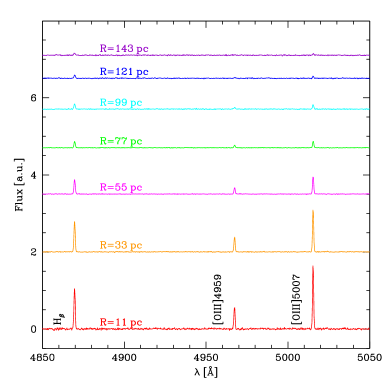
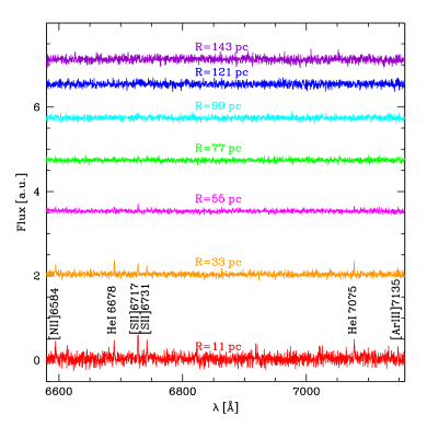
Figure 11: Left: zoom view between 4850 and 5050 Å of the 1-spaxel equivalent LR-B spectra of the ionization rings. Each spaxel spectrum is shifted in the Y-axis for the sake of clarity. The spectrum of each ring is plotted in a different colour, whose label indicates the distance from the central brightest spaxel. Right: equivalent figure for LR-R but we deliberately omit the H${\alpha}$ region to show other very faint lines between 6575 and 7150 Å.

The fluxes of H${\alpha}$, H${\beta}$ and [O iii] 5007, divided by the corresponding flux in the brightest spaxel, are shown in Fig. 9. As expected, the flux of each line increases when the aperture is larger. In contrast, the ratio of [OIII] 5007/H$\beta$, shown in the right panel, decreases as the size of the region increases. The dilution of this ratio with the galactocentric distance, if confirmed in other XMD galaxies, might point to a selection effect as the integrated detected [OIII] 5007/H$\beta$, extensively used to extract the XMD galaxies samples, could be linked not only to the metal content itself but also to the distance to the galaxy, in other words, to the spatial resolution.

For the LR-R setup, the addition of the spectra from the two first rings to the central spectrum, was particularly useful to increase the flux as the lines are not strong. This is illustrated in Fig. 10, where we present, besides H$\alpha$, the regions of the spectra for [NII] 6584, HeI 6678, [SII] 6717, 6731, HeI 7075 and [ArIII] 7135. This method allow us to see and to measure these lines even with the uncertainties shown in Table 2. However, adding more rings dilutes the weak lines increasing the noise (see Table 2) so that, given the uncertainties, we can assume that for these weak lines the central plus the two first rings values correspond to the global/integrated spectrum for the complete region of 140 pc.

In our observations the spectral coverage is provided by the wavelength range of LR-B and LR-R, as we do not have data in between. In addition, the data might have a slightly different absolute flux calibration, despite clear observing conditions were reported by the observatory staff for the observations in both setups. To verify the general calibration in LR-B, we have compared the H${\beta}$ flux measured in our image with the reported fluxes by H16. On the one hand, in their observations at KPNO, for a slit of 3.21 arcsec length and 1.5 arcsec width, these authors give a value of (18.70 $\pm$ 0.30$)\,\times$10^-16 erg cm^-2 s^-1. This aperture is slightly smaller than our total 63 spaxels aperture, for which we measure a value for of H${\beta}$ flux of (16.07 $\pm$ 0.06) $\times$ 10^-16 erg cm^-2 s^-1. Assuming an absolute flux calibration error of 10 percent these measurements are coherent. On the other hand, with the MMT and a slit of 2.70 arcsec $\times$ 1 arcsec and seeing of 1.00 arcsec, they report a value of (8.31 $\pm$ 0.17) $\times$ 10^-16 erg cm^-2 s^-1. We simulated the MMT slit in the qla tool and extracted the corresponding spectrum, measuring a flux of 7.56 $\times$ 10^-16 erg cm^-2 s^-1, that is also coherent with the MMT value within 10 percent. This comparison allows us to validate the LR-B calibration.

To verify the calibration in the LR-R setup we followed the same approach, i.e. we simulated the MMT slit in the LR-R image, extracted the spectrum and derived the value of H${\alpha}$ flux. H16 reported for their slit a value of the emission line fluxes ratio between H${\alpha}$ and H${\beta}$ of 2.7663 while we obtain 3.6402. It is hard to say if these numbers are consistent within 10 percent or if we have a real increase of the flux in LR-R by a factor of 1.3 (3.6402 / 2.7663). For this reason we decided to compute the ionization budget from the luminosity of H${\beta}$ (see Section 5).

Table 3: LR-B emission lines measurements in different ionization rings from the central brightest spaxel. Fluxes are given in units of $\times$ 10^-17 erg cm^-2 s^-1.

(1)	(2)	(3)	(4)	(5)	(6)	(7)	(8)	(9)	(10)	(11)	(12)	(13)
d	d	nr	Ns	H${\beta}$	H${\beta}$	H${\gamma}$	H${\gamma}$	[O iii]4363	[O iii]4959	[O iii]5007	He i4471	He i5015
pc	”			Flux	EW (Å)	Flux	EW (Å)	Flux	Flux	Flux	Flux	Flux
11	0.31	0	1	10.50$\pm$1.03	213$\pm$168	5.09$\pm$1.45	44$\pm$43	0.38$\pm$0.44	5.18$\pm$0.73	14.42$\pm$1.06	0.26$\pm$0.26	0.20$\pm$0.17
33	0.93	1	6	7.87$\pm$0.44	339$\pm$193	3.91$\pm$0.58	21$\pm$ 8	0.24$\pm$0.17	3.55$\pm$0.37	9.95$\pm$0.44	0.41$\pm$0.13	0.14$\pm$0.07
55	1.55	2	12	3.91$\pm$0.24	116$\pm$ 43	2.21$\pm$0.39	15$\pm$ 5	0.17$\pm$0.13	1.53$\pm$0.12	4.34$\pm$0.20	0.11$\pm$0.08	0.05$\pm$0.04
77	2.17	3	18	1.67$\pm$0.11	41$\pm$  9	1.24$\pm$0.21	8$\pm$ 2	–	0.64$\pm$0.07	1.63$\pm$0.10	–	–
99	2.79	4	8	1.42$\pm$0.13	19$\pm$  4	0.94$\pm$0.28	4$\pm$ 1	–	0.48$\pm$0.07	1.15$\pm$0.12	–	–
121	3.41	5	6	1.00$\pm$0.11	17$\pm$  4	0.46$\pm$0.28	3$\pm$ 2	–	0.22$\pm$0.09	0.43$\pm$0.09	–	–
143	4.03	6	4	0.66$\pm$0.16	16$\pm$  9	0.42$\pm$0.34	2$\pm$ 2	–	0.09$\pm$0.08	0.37$\pm$0.11	–	–

Figure 12: Radial dependence of the observed flux (left) and EW (right) of the three Balmer lines present in the LR-B and LR-R spectral ranges.

Here, we briefly discuss the gas properties derived from the emission line spectrum. The low metallicity of this galaxy produces a large value of $T_{\rm e}$ as derived from the [O iii] 4363, 4959, 5007 emission lines. Due to the low S/N of the [O iii] 4363 line in our data, we have derived $T_{\rm e}$ only in a central aperture adding 7 spaxels (the brightest one + 6 around) equivalent to a radius of 33 pc. We used the $R_{\rm O3}$ ratio, (I [O iii] 4959 + I [O iii] 5007) / I [O iii] 4363, with a value of 52.18 $\pm$ 32.24, and derived $T_{\rm e}$ according to equation 5 from Pérez-Montero (2014), obtaining a value of 17 284 $\pm$ 5 789 K. The intrinsic weakness of [O iii] 4363 and the associated error bars as large as 50 percent make difficult to have a more accurate determination. This value of $T_{\rm e}$ is consistent within the errors with the value of 19 130 $\pm$ 800 K from Cannon et al. (2011). We tried to calculate the value of $n_{\rm e}$ in the same central aperture from the ratio $R_{S2}$ = I [S ii] 6717 / I [S ii] 6731, following equation 2 in Pérez-Montero (2014), obtaining 1.59 $\pm$ 0.49 compatible with a low density regime, $n_{\rm e}$ < 40 cm^-3, for the derived $T_{\rm e}$. However, the error in $n_{\rm e}$ due to the low S/N of [S ii] 6717, 6731 lines makes impossible to obtain a better determination from our data. H16 did not present a more accurate estimate, giving a value in an equivalent aperture of $270\pm 200$ cm^-3.

4.4 Emission lines throughout the ionized region

We also identified the spaxels with emission in the different ionization rings around the central brightest spaxel, and averaged the spectra of all these spaxels, to make the measurement equivalent to one spaxel. The resulting spectrum for each ring is displayed in Fig. 11 where a zoom view into regions of the spectrum in LR-B (left) and LR-R (right), are plotted in a different colour with a label, indicating the distance from the central brightest spaxel, using the scale factor of 22 pc spaxel^-1.

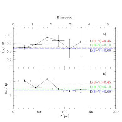
Figure 13: Radial dependence of the Balmer lines ratios. The plot shows three lines with the theoretical ratios after applying a certain value of reddening, $E(B-V)$, as labelled in the plot.

Figure 14: Radial dependence of some emission lines from LR-B spectra. a) [OIII] 4969+5007/H$\beta$; b) [OIII] 5007/H$\beta$; c) [OIII] 4363/H$\beta$; d) HeI 4471/H$\beta$; and e) HeI 5015/H$\beta$.

Table 3 presents the results for the emission lines in the LR-B spectra. The first four columns are: (1) the distance from the central brightest spaxel to the ionized ring, (2) the same distance in arcsec, (3) the identification of the ionized ring, being 0 the central spaxel and considering 22 pc between two consecutive rings and (4) the number of spaxels in the averaged spectrum. Values in columns 5, 7, 9, 10, 11, 12 and 13 are the observed fluxes, with their corresponding errors, in units of $\times$ 10^-17 erg cm^-2 s^-1 for H${\beta}$, H${\gamma}$, [O iii] 4363, [O iii] 4959, [O iii] 5007, He i 4471 and He i 5015. The EW of H${\beta}$ and H${\gamma}$ with their errors are displayed in columns 6 and 8, respectively. In the case of the LR-R setup, with the exception of H${\alpha}$, the results for the measurements of emission lines per spaxel as a function of the distance from the brightest one, are not included in this section due to the low S/N, as illustrated in the right panel of Fig. 11. Nevertheless, as we have shown in the previous section, by accumulating data of different apertures we were able to measure some of these lines.

Fig. 12 shows the Balmer lines fluxes (left), and their corresponding EW (right), as a function of the distance from the brightest spaxel. A clear decrease appears in both panels, although the EW of H$\beta$ shows a maximum in the second ring. In Fig. 13 we plot the measured Balmer ratios H${\gamma}$/H${\beta}$ (top) and H${\alpha}/$H${\beta}$ (bottom). We overlaid the theoretical values for $T_{\rm e}$ = 20000 K and three values of the reddening, $E(B-V)$: 0.00, 0.10 and 0.45 mag with different colors as labelled. The extinction seems closer to the red line $E(B-V)$ = 0.45 for some rings, while is near $E(B-V)$ = 0 for others, so the averaged value is $<$E(B-V)$>$ $\sim 0.23$ mag, in agreement with the one given by MQ20 of 0.29 mag. Fig. 14 presents the radial dependence of the ratio of some LR-B emission lines over H${\beta}$ as a function of the distance from the brightest spaxel. We measured only for the three central rings, except for [OIII] 5007, 4969 obtained, as the Balmer lines, up to 140 pc of distance from the central spaxel.

5 DISCUSSION

5.1 Constraining the parameters of the ionizing population

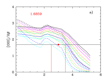
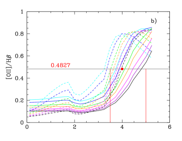
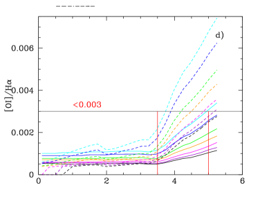
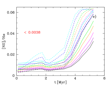
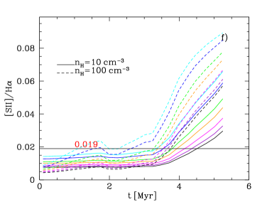
Figure 15: Evolution of the emission line ratios from popstar models (M10) of Z$=0.0004$ with Salpeter IMF (taken 0.15 and 100 M_$\sun$ as lower and upper mass values). The models for different values of the cluster mass are plotted in colors as labelled in panel c. Solid and dashed lines correspond to models with n_e of 10 and 100 cm^-3, respectively, as labelled in panel f. We have included as red dots, and labelling the numerical values, the measurements for the central region taken from H16.

We dedicate this section to interpret the results of the detailed spatially-resolved study of the gas emission line spectra and kinematics presented in section 4. The first task is to constrain the metallicity, mass and age of the dominant young stellar cluster responsible for the ionization. To this aim we take as input: (1) the ionized gas properties obtained from the emission line spectrum, such as $T_{\rm e}$, $n_{\rm e}$ and abundance, derived in the central region, (2) the emission line ratios diagnostics in the same region, (3) the number of ionization photons, $Q(H)$, in the nebula and (4) the geometry of the region as seen in the MEGARA maps together with the information of the HST images from MQ20.

We assume the same metallicity Z, and in particular the same oxygen abundance, for both gas and stars of the ionizing cluster. Taken the value of $T_{\rm e}$ from the [O iii] emission lines, the value of 12 $+$ log(O/H) is between 7.02 (H16) and 7.12 (MQ20). Considering 8.69 as the solar value, the metallicity, Z, would be in the range 0.021 Z_$\sun$ $\leq$ Z $\leq$ 0.030 Z_$\sun$. As the solar metallicity is Z $=$ 0.017, the value of the metallicity for Leoncino would be 0.0004 $\pm$ 0.00008, so that for all comparisons in this paper with popstar models, we will use those corresponding to Z $=$ 0.0004.

We calculate the number of ionizing photons from the H$\beta$ luminosity, as:

$${Q(H)}=2.10\times 10^{48}\,\mathrm{L(H{\beta}),}$$ (1)

where L(H$\beta$) is the luminosity of H$\beta$, in units of 10³⁶ ergs s^-1 calculated from the flux assuming a distance to the galaxy. We take the flux of H$\beta$ measured in our LR-B image for all the 63 spaxels, which is 16.07 $\times$ 10^-16 erg cm^-2 s^-1. Considering the scale of 22 pc spaxel^-1 (corresponding to a distance of 7.7 Mpc) we measure a L(H${\beta}$) total value of $1.140\times 10^{37}$ erg s^-1 ($\log$ L(H${\beta}$) = 37.06) and a derived number of ionizing photons of 2.39 $\times$ 10⁴⁹ s^-1 ($\log\,Q(H)$ = 49.38).

We assume that the gas is ionized by the most massive stars of a young SSP, whose properties should be derived from the gas emission line spectrum. popstar evolutionary synthesis models (M09) generated, for a given IMF and a set of the ionizing cluster parameters, age and metallicity, the SEDs with the shape of the ionizing continuum, the number of ionizing photons and the inner radius of the Hii region, $R_{\rm{in}}$, set by the action of the cluster mechanical energy. popstar models are the only ones computed for very low metallicity young populations, dominated by the massive stars ionizing spectrum. These models are given for a cluster mass of 1 M_$\sun$. Hence, the luminosity and $Q(H)$ have to be scaled with the actual cluster mass (in M_$\sun$) while the radius of the ionizing shell with M_$\sun$^0.2 (see M09).

We used the estimated value of $Q(H)$ and the results from those popstar models to infer the mass of the dominant ionizing cluster. M09 models predict values of 46.75, 46.58, 46.19 and 45.88 s^-1 M_$\sun$^-1 when using the IMF from Chabrier (2003), Salpeter (1955), Kroupa (2001) and Ferrini, Penco and Palla (1990) respectively, at 3.2 Myr, and 46.71, 46.52, 46.16 and 45.85 at 3.5 Myr. The total value of log $Q(H)$, when adding all spaxels (63) with detected emission in H$\beta$, is 49.38 s^-1. Assuming that all these photons are produced in a single ionizing cluster, the mass derived when using different IMFs ranges from 0.4 to 3.4 $\times$ 10³ M_$\sun$. We therefore conclude that, on the basis of the models and assuming an ionization bounded region, and no photon escaping from the nebula, the ionizing cluster mass is $\approx$1.7 $\times$ 10³ M_$\sun$, with an uncertainty of a factor of 2 including all hypotheses (IMF, reddening, and age, among others). We have to take into account that the uncertainty in $Q(H)$ derived from stellar population synthesis models is large, since for a given cluster mass, $Q(H)$ depends not only on age and metallicity but overall on the selected IMF, and in the case of small clusters on possible stochastic effects, too. Furthermore, there is an uncertainty in the distance, e.g. assuming a distance of 13.8 Mpc, the upper limit estimated by MQ20, the spaxel size and the L(H${\beta}$) would increase up to a factor of 1.9 and 3.2, respectively.

The number of ionizing photons is derived not only from the value of L(H${\beta}$), which depends on the assumed distance to the galaxy, but also from the predictions of the synthesis evolutionary models. These models have general uncertainties common to any metallicity, e.g. the IMF –number of massive stars formed– and the assumed isochrones and atmosphere models. These assumptions can change the number of ionizing photons up to a factor of 3. Moreover, the poor understanding of the evolution and atmospheric properties of low metallicity stars, add more uncertainty to the predictions for stellar populations of XMD galaxies.

We have not considered any reddening when deriving $Q(H)$ as we have shown that the Balmer ratios are consistent with very low values of $E(B-V)$, see Fig. 13.

M10 used popstar models and the photoionization code cloudy (Ferland et al., 1998) to predict the emission line spectrum produced by an ionizing SSP under certain hypotheses on the chemical composition of the gas (abundance and electron density) and an ionization bounded geometry. We used the published results from M10 for models at Z $=$ 0.0004 (0.023 Z_$\sun$), at all ionizing ages and the two values of $n_{\rm e}$ (10 and 100 cm^-3) they used in the published models, to constrain the cluster parameters. As a reminder of the models reliability, M10 showed that the abundances derived from the computed emission line spectra through the [O iii] electron temperature differ from the input metallicity in the model less than 0.05 dex in the range 0.0001 $\leq$ Z $\leq$ 0.008. Fig. 15 shows the evolution up to 6 Myr of six emission line ratios from M10 for Z $=$ 0.0004 with a Salpeter IMF (taken 0.15 and 100 M_$\sun$ as lower and upper mass values). The models have cluster masses of 0.12, 0.20, 0.40, 0.60, 1.00, 1.50 and 2.00  $\times$ 10⁵ M_$\sun$, plotted in different colors as labelled in panel c. Solid and dashed lines correspond to models with $n_{\rm e}$ of 10 and 100 cm^-3, respectively. The emission line ratios are [O iii] 4959+5007/H$\beta$, [O ii] 3727+3729/H$\beta$, [O ii]/[O iii], [O i] 6300/H$\alpha$, [N ii] 6584/H$\alpha$ and [S ii] 6717, 6731/H$\alpha$. For comparison purposes, we included the measurements for the central region taken from H16 (1.6859, 0.4827, 0.2863, < 0.003, < 0.0038, and 0.019, plotted as red dots in panels a, b, c, d, e and f, respectively). We used H16 data because on the one hand, they are equivalent to our central 7-spaxel aperture, and for all lines present in both, H16 and this work, the intensity values are consistent within the errors, see section 4.3. On the other hand, H16 measured [O ii] 3727, 3729, very useful to constrain the gas density and the hardness of the ionizing radiation, but we could not measure it given the LR-B wavelength coverage.

We compared the observed line ratios with the models for the smallest cluster (represented by the cyan lines), which is about one order of magnitude larger than the one we derive from the luminosity of H$\beta$. The values of [O iii]/H$\beta$ (panel a) and [O ii]/H$\beta$ (panel b) points to an age of 3 – 4 Myr, although younger ages would be still compatible for higher values of electron density or less massive clusters (remember that in this case the electron density is $<40$ cm^-3). The observed ratio [$\text{O\,{ii}}]/[\text{O\,{iii}}$] (panel c) is compatible with the low density curves for clusters older than 3 Myr. The values of both [O i] 6300/H$\alpha$ (panel d) and [N ii]/H$\alpha$ (panel e) fit the models with $n_{\rm e}$ =10 cm^-3 only. Finally, the value of [S ii] 6717, 6731/H$\alpha$ (panel f) discards a low-mass ionizing cluster in a high density regime (dashed cyan line) and predicts an age between 4 and 5.5 Myr.

The EW(H$\beta$) can also constrain the ionizing cluster age in this central region. popstar models predict a value of 250 $\pm$ 50 Å for ages between 3 and 5 Myr at Z $=$ 0.0004 and a Salpeter IMF. If we consider any other IMF used in M09 models, we obtain a similar cluster age within $\pm$ 1 Myr. Despite our measurement of EW(H$\beta$) in the central aperture has a large error, 306 $\pm$ 136 Å , see Table 1, this result is compatible with the predicted value by M09 for the derived cluster age. In summary, the placement of the observed values of the central region of Leoncino in the emission-line evolutionary diagrams and the measurement of the EW(H$\beta$) are all coherent with a metallicity of Z $=$ 0.0004, an age of 4.0 $\pm$ 1.0 Myr for the ionizing cluster and low-density ($\approx$ 10 cm^-3).

The equilibrium time scale increases as the metallicity decreases due to the low content of metals that can cool the gas. In addition, the effect is strengthened with decreasing hydrogen density. For this reason, we need to outline the importance of considering the equilibrium time of the photoionized nebula that, in low-metallicity galaxies, like Leoncino, is of the same order of magnitude as the age of the ionizing cluster. The time-step in popstar models corresponds to the stellar cluster age step given by the isochrone time resolution. However, the output of the photoionization models shows the picture of the ionized region once the equilibrium state is reached. This implies that when we observe an ionized region, what we really see is the effect of an ionizing cluster of a given age, regardless the actual age of the ionized nebula. The consequence is that the age resolution with which we can date the ionizing cluster from the information of the gas ionizing spectrum depends on the speed at which the nebula reaches the equilibrium. In practice, this means that the ionizing stellar cluster would be older when we observe the region than the age we infer from the emission-line spectrum, since the cluster will have evolved during the nebula equilibrium time, controlled by its metallicity.

Table 4: popstar $+$ cloudy models at Z $=$ 0.0004 assuming $n_{\rm e}$ $=$ 10 cm^-3 for Leoncino.The table shows the first rows of the full table presented in the Appendix.

(1)	(2)	(3)	(4)	(5)	(6)	(7)	(8)	(9)	(10)	(11)	(12)	(13)	(14)
EW(H$\beta$)	$\log$ Q(H)∗	log age	$\log$ Q(H)	$\log$ Rin	[O ii]	[O ii]	H$\gamma$	[O iii]	[O iii]	[O iii]	H$\alpha$	[S ii]	[S ii]
Å	s-1M$\sun$-1	yr	s-1	cm	3726	3729	4340	4363	4959	5007	6563	6717	6731
415	46.66	6.30	50.00	19.55	0.1608	0.1088	0.4759	0.0391	0.5021	1.4980	2.8252	0.0270	0.0190
415	46.66	6.30	49.95	19.55	0.1654	0.1119	0.4759	0.0382	0.4939	1.4736	2.8258	0.0277	0.0195
415	46.66	6.30	49.90	19.55	0.1701	0.1151	0.4758	0.0372	0.4855	1.4486	2.8266	0.0284	0.0200
415	46.66	6.30	49.85	19.55	0.1749	0.1184	0.4758	0.0363	0.4770	1.4230	2.8272	0.0292	0.0205
415	46.66	6.30	49.80	19.55	0.1800	0.1218	0.4758	0.0353	0.4683	1.3971	2.8280	0.0300	0.0211
…	…	…	…	…	…	…	…	…	…	…	…	…	…

M10 tested this effect by obtaining the equilibrium time for each cloudy model. They concluded that neither the total number of ionizing photons (cluster mass) nor the ionizing spectrum shape (cluster age) have a significant role in setting the equilibrium time (actual age) of the ionized regions, which is mainly controlled by the electron temperature (given by the metallicity). According to those results, the average equilibrium age, t_eq is reached around 13.6 and 3.1 Myr for metallicities Z $=$ 0.0001 and 0.0004 in popstar + cloudy models. This implies that, at such low metallicity, there is a delay between the actual time when we observe the ionized region and the age of the stellar cluster responsible for this ionization. At Z $=$ 0.0004, this delay is of the order of 3 Myr, and therefore, we could observe low-metallicity regions apparently and in practice ionized by a young cluster, but without finding the expected young and hot stars when we observe directly inside the nebula, just because they have evolved. Moreover, we could find more evolved stars radiating in the IR as RSGs (with an age between 6.5 to 7.5 Myr at Z = 0.004) as the resulting products of the evolution of the ionizing stars that can produce, among other effects, a decrease of the values of the EW of Balmer emission lines. All these effects complicate considerably the determination of the stellar populations in low metallicity and even more at low-density environments.

Summarizing all the previous constraints, from the comparison between the observations and popstar models and assuming an ionization bounded region and a low electron density ($\approx$10 cm^-3), we obtain that a cluster with mass of young stars of $\approx$ 1.7 $\times$ 10³ M_$\sun$, with an uncertainty of a factor of 3, a metallicity around or slightly lower than Z = 0.0004, and an age of 4 $\pm$ 1 Myr, is responsible for the ionization. At this metallicity, the time for the nebula to reach the equilibrium is $\approx$ 3 Myr, implying that the ionizing cluster would have an age of 6 $\pm$ 1 Myr at the time of observing the ionized nebula. At this age, popstar models (Padova’s isochrones) predict the appearance of RSG and their absorption Balmer lines would produce a decrease of the effective emission EW measured in the region.

5.2 Possible scenarios for the observed ionization structure

The strength and novelty of MEGARA is the capability of mapping the actual gas distribution with spatial resolution. This has allowed us to measure, for the first time, the total flux of the Balmer lines in emission and to produce maps in different emission lines ratios, unveiling the ionization structure of the galaxy and the region kinematics, as discussed in sections 4.1 and 4.2, respectively. From both, the published data and our MEGARA observations, we know that a young ionizing cluster is required to reproduce the observed emission line spectrum of the gas at least in the central two rings around the brightest spaxel. In this section we explore different scenarios that could explain simultaneously the central emission line spectrum and the spatial distribution of [O iii]/H$\beta$ and the EW(H$\beta$), whose values are summarized in Table 3.

5.2.1 popstar + cloudy models

We carried out this task by comparing our data with the output of the photoionization code cloudy, assuming Leoncino metallicity and an ionization bounded geometry, and considering that the ionizing source is a popstar SSP. These models generate the SED of an ionizing cluster, of a certain mass, age and metallicity, which would have been formed in a very short time scale, comparing with the current evolutionary age, and would be physically concentrated in the center of the region. The winds and supernova produced by the most massive stars would push the neutral gas, placing it at a certain distance, $R_{\mathrm{in}}$, where the photons would start to ionize that gas. The resulting geometry would be a plane-parallel cell of ionized gas from $R_{\mathrm{in}}$ to a distance $R_{\mathrm{out}}$, with a thickness, $\Delta$R. The photoionization models assume that the region is not limited by the amount of neutral gas to be ionized but by the number of ionizing photons, i.e. the ionization bounded scenario. The metallicity controls the ionized region evolution until reaching the equilibrium in the nebula, and cloudy stops the computation as soon as the nebula has been cooled.

Under these assumptions García-Vargas, Mollá, Martín-Manjón (2013, hereafter GV13) published the results from a grid of popstar + cloudy simulations for an age range between 1 and 5.4 Myr, two values of the electron density, 10 and 100 cm^-3, and six values of the metallicity, considering the same abundance for gas and stars. GV13 also concluded that the emission line spectrum of elements heavier than hydrogen is not produced under the same geometry by older clusters, up to 20 Myr, which however still produce Hii regions, with large envelopes of Balmer lines in emission, as the gas is pushed further by the mechanical energy of winds and SNe. The SEDs of these clusters can ionize hydrogen, but the high-energy photons are missing. The combination of the two effects, lack of hard photons and large distance between the cluster and the pushed gas, produces very low values of the ionization parameter, preventing the emission line spectrum of elements heavier than hydrogen.

For this paper we produce a customized popstar + cloudy grid of models with a global metallicity for gas and stars of Z $=$ 0.0004 and considering that the abundances of the different elements are those derived from the emission line spectrum of the central region of Leoncino. All models assume an $n_{\rm e}$ $=$ 10 cm^-3. The results are given in Table 4 where we only show the first rows while giving the full table in the appendix. We run 631 different models resulting of the ionization by clusters of ages (in logarithm) of 6.30, 6.35, 6.40, 6.44, 6.48, 6.51, 6.54, 6.57, 6.60, 6.63, 6.65, 6.68, 6.70, 6.72, 6.74, 6.90, 7.15 and 8.35, corresponding to ionizing clusters with ages between 2 and 5.5 Myr, plus some non-ionizing clusters at 8, 12.5 and 223 Myr as an example of older populations. The grid covers a range in the logarithm of $Q(H)$, corresponding to a cluster mass range, that produces models with different value of the ionization parameter. Table 4 shows, for each model, the value of the EW of H$\beta$ (in Å column 1), the logarithm of the number of ionizing photons (s^-1) per solar mass (column 2) corresponding to the cluster age (column 3, logarithm, in yr), the total number of ionizing photons in s^-1 (column 4) and the value of the inner radius, $\log$ $R_{\mathrm{in}}$ (columns 5). These five first columns come from the popstar SSPs. Columns 6 to 14 display the emission line ratios normalized to H$\beta$ intensity of [O ii] 3726, 3729, H$\gamma$ 4340, [O iii] 4363, 4959, 5007, H$\alpha$ and [S ii] 6717, 6731.

Given the lack of firm evidence for the presence of escaping gas through a disrupted nebula discussed in section 4.2, we cannot determine whether ionizing photons are escaping from the nebula. Thus, for the sake of simplicity, we assumed an ionization bounded nebula with no ionizing photons being able to escape from it. In the following sections we discuss different scenarios to explain the observed ionization structure. The ionization parameter does not depend on the assumed distance to the galaxy, so neither the main conclusions reached in the next subsections.

5.2.2 Scenario 1: a single young cluster is responsible for observations

The first scenario is based on having a single young cluster with the values of mass, age and metallicity derived in section 5.1 as responsible for all the ionizing photons. Therefore, we should reproduce the observed size of the ionized region, ranging from 22 pc (at the the center) to $\approx$ 150 pc. We explore this scenario under different hypotheses on mass cluster and gas distribution.

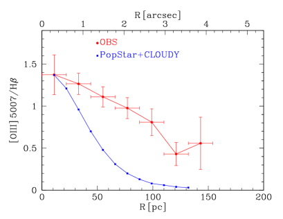
Figure 16: Values of [OIII] 5007/H$\beta$ as a function of the distance from the center of the ionized region. The results obtained from the popstar+cloudy models, assuming a single SSP as ionizing source and an uniform gas distribution throughout the nebula are shown in blue. The values and error bars derived from MEGARA observations are shown in red.

As a first attempt, we assume that a small ionizing cluster of mass $\approx$ 1.7 $\times$ 10³ M_$\sun$, estimated from the ionization budget from L(H$\beta$), is responsible for the ionization. The mechanical energy from winds and supernova would push the gas placing at $R_{\mathrm{in}}$ of 29 pc, the size of the central spaxel at this scale. To test this hypothesis, we use the results from GV13 models. We find that for such a low value of the mass cluster, these models predict $R_{\mathrm{out}}$ smaller than 40 pc at all ionizing ages, in disagreement with the observed size of the ionization region of $\approx$ 150 pc. The first conclusion is that we cannot reproduce a region with a very small $R_{\mathrm{in}}$ and a relatively large $R_{\mathrm{out}}$ for a low mass SSP, assuming that the distance to $R_{\mathrm{out}}$ is a consequence of the mechanical energy of this single small ionizing cluster exclusively.

A second approach within this same scenario, a single cluster responsible for the ionization structure, is to assume that we might somehow have underestimated the number of ionizing photons, so that we would have a more massive cluster. Published models for a young cluster between 3 and 5 Myr at Z $=$ 0.0004 (see Table 1 of GV13) give values of R_in, $\Delta$R and R_out of 42, 46 and 88 pc (at 3 Myr), and 89, 3 and 92 pc (at 5 Myr) for a cluster of 1.2 $\times$ 10⁴ M_$\sun$, the lowest mass of these published models. These values increase to 73, 247 and 320 pc (at 3 Myr) and 156, 16, 173  pc (at 5 Myr) for a cluster of 2 $\times$ 10⁵ M_$\sun$, the upper mass edge for the models presented in that paper. Scaling the models to more massive clusters, we obtain that a 3.5 $\pm$ 0.5 Myr cluster with a mass of 5 $\pm$ 1 $\times$ 10⁴ M_$\sun$ reproduces the size of the ionized region, with an inner radius of 30 $\pm$ 5 pc and an outer radius of 140 $\pm$ 10 pc. However, for such as massive cluster, the logarithm of $Q(H)$ is 51.1 $\pm$ 0.1, much larger than our estimated value of 49.38, for the total ionized nebula. This mass difference is too high to be explained by distance estimate errors, a different IMF and/or intrinsic evolutionary model uncertainties. To explain that difference we would need a very large escaping fraction of photons of the region (98 per cent), leaving only 2 per cent of the produced photons to ionize the gas. From the kinematics study presented in section 4.2, there is no evidence at all of an enormous photon loss.

We also explore a different geometry: instead of having the gas placed at a certain distance as resulting of the mechanical energy effect of the ionizing cluster, we consider that there is gas at all distances from the cluster, still located at the center of the region. This would be equivalent to having a superposition of ionized layers, each one corresponding to a different value of the ionization parameter, which decreases with the square of the distance between the ionizing source (the cluster) and the boundary of the ionized region. For this simulation we considered a SSP with $\log$ t $=$ 6.54 (3.5 Myr) and $\log$ $Q(H)$ $=$ 49.99. We run ionization bounded models by changing the value of the inner radius from 11 to 132 pc in steps of 11 pc. Fig.16 presents the ratio [O iii]/H$\beta$ observed (in red) and the models (in blue). We see that the observations cannot be reproduced either. A similar result would be obtained with a density gradient model, with the density decreasing outwards, since this would also decrease the ionization parameter. However, we do not have reliable measurements of density sensitive emission lines to be compared to the models.

Therefore, the conclusion is that a single ionizing young cluster cannot reproduce simultaneously $Q(H)$ derived from L(H$\beta$) and the size of the ionized region in an ionization bounded geometry and no photons escaping from the nebula.

5.2.3 Scenario 2: coexistence of two ionizing clusters

Table 5: Mass, $R_{\rm in}$, $\Delta R$, $R_{\rm out}$ and ionization parameters from popstar model for an intermediate age cluster (6-20 Myr) at Z = 0.0004 assuming $n_{\rm e}$ = 10 cm^-3.

Age	$Q(H)$/M$\sun$	Mass	$R_{\mathrm{in}}$	$\Delta R$	$R_{\mathrm{out}}$	log u
Myr	s-1/M$\sun$-1	103 M$\sun$	pc	pc	pc
6	45.80	1.2	67.1	0.8	67.9	-4.33
7	45.61	1.9	83.5	0.4	83.9	-4.52
8	45.43	2.8	97.9	0.2	98.1	-4.66
9	45.29	3.9	113.1	0.2	113.3	-4.78
10	45.01	7.4	139.7	0.1	139.8	-4.97
15	44.16	52.5	269.9	0.0	269.9	-5.54
20	43.74	138.0	386.1	0.0	386.1	-5.85

The second scenario assumes that the observed structure is the result of the combination of the actions of a very young cluster, responsible for the ionization of the two central rings, plus a few Myr older cluster, still capable to reproduce the ionization structure that we detect in [O iii], H$\beta$ and H$\alpha$. Both clusters would be located at the center of the ionized region. In this case, the youngest cluster would be responsible for the ionization detected in the first two rings only, which contain 68 percent of the total H$\beta$ flux as shown in Table 3, while the rest of the H$\beta$ flux (32 percent) would come from the ionization of the older cluster. This would give us values of $\log$  $Q(H)$ of 49.21 and 48.88 for the young and the old cluster, respectively.

The mass of the young ionizing cluster, with an age of 3.5 $\pm$ 0.5 Myr, would be (0.75 $\pm$ 0.3) $\times$ 10³ M_$\sun$. This cluster mass would be coherent with the size of the central ionized region 50 $\pm$ 20 pc  and cloudy simulations reproduce the central emission line spectrum.

For the older population, we summarize popstar results in Table 5 for metallicity Z $=$ 0.0004 and $n_{\rm e}$ = 10 cm^-3. Column 1 gives the cluster age in Myr, column 2 is the logarithm of $Q(H)$ for a cluster with 1 M_$\sun$, column 3 is the actual cluster mass corresponding to the value of $\log$ $Q(H)$ $=$ 48.88, columns 4, 5 and 6 give the inner radius, the region thickness and the outer radius (all in pc) of the ionized nebula. Lastly, column 7 gives the ionization parameter, calculated from $Q(H)$, $n_{\rm e}$ and $R_{\mathrm{in}}$.

We find that there is a range in age 8 $\pm$ 2 Myr and mass (4.5 $\pm$ 3.0) $\times$ 10³ M_$\sun$ for the clusters, which can simultaneously reproduce $Q(H)$ and the region size. We run cloudy models for such a cluster. The conclusion is that this cluster can explain the extended region in H$\beta$ and H$\alpha$ but cannot reproduce the observed values of [O iii] across the nebula, due to the low values of the ionization parameter, neither consequently the large [O iii]/H$\beta$ measured at large distances from the ionizing cluster(s).

5.2.4 Scenario 3: one or several young clusters evolving while reaching region equilibrium time

This scenario considers that we have either, a single ionizing young cluster evolving while the nebula reaches the equilibrium time or several small clusters at different locations throughout the nebula resulting from mass segregation.

In the first case and considering that the region t_eq $\approx$ 3 Myr for Leoncino low metallicity, the ionization would be the result of the photons produced by the evolving cluster until reaching t_eq and being cooled so that approximately between 3.5 and 6.5 Myr.

In the second case, we can expect some mass segregation throughout the region, producing smaller star associations along the nebula that could also explain the observed gradients. In fact, we could have both phenomena simultaneously. The ionization structure would be equivalent to have several very young clusters of different ages, which are ionizing the gas in different locations of the nebula. The observed emission line spectrum would then be the result of the combination of the effects from the different clusters producing a series of ionized layers. We have explored this assumption by plotting in Fig. 17 the results of the ratio [O iii] 5007/H$\beta$ as a function of the logarithm of the age of the SSP (in yr), obtained from the customized popstar+cloudy models described in subsection 5.2.1. Models are plotted as dots and we have overlaid the observed values of [O iii] 5007/H$\beta$ as solid lines, using different colours to distinguish the observations at different distances from the central spaxel (in red) to the outer zones (in dark blue and purple). The observations can be reproduced with SSPs of ages between 6.3 and 6.8 (in $\log$ t).

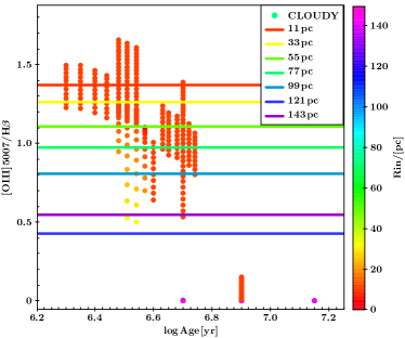
Figure 17: The resulting [O iii] 5007/H$\beta$ as a function of the logarithm of the age as obtained from the set of cloudy models shown as a scale in terms of R_in (in pc) given at right, with our observed data for this ratio of lines with different colors as labelled.

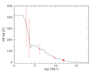
Figure 18: The evolution with time of EW(H$\beta$) as computed in popstar models compared with the results obtained in this work for different rings. The points give the possible age of each cluster in each ring.

This scenario is also consistent with the measurements of the EW(H$\beta$), as it is shown in Fig. 18. The theoretical values (black curve) of EW(H$\beta$) from popstar SSPs has been plotted as a function of the cluster age. The observations at different distances from the center (red points and error bars) have been overlapped. The distribution is compatible with the coexistence of several clusters of different ages. Nevertheless, the large error bars in the EW(H$\beta$) data, due to the low signal in the continuum, do not allow us to discriminate between having several young clusters with different ages, from having a single or multiple ionizing clusters and a much older stellar population in the bulge of the galaxy, which would produce the same dilution effect of the H$\beta$ emission line and the decreasing of its equivalent width.

6 Summary and Conclusions

We present for the first time spatially resolved spectroscopy of the low-metallicity galaxy AGC 198691 (Leoncino Dwarf) obtained with the IFU of MEGARA at GTC, using the VPH gratings LR-B (4304 – 5198 Å) and LR-R (6098 – 7306 Å) with resolving power R $\approx$ 6 000. The spatial resolution is 22 pc spaxel^-1, assuming a distance to Leoncino of 7.7 Mpc. The emission line spectrum in the central region confirms the published data.

We obtained maps for the brightest emission lines and measured the first momenta (flux, velocity, sigma), detecting H$\alpha$, H$\beta$ and [O iii] emission with S/N $>$ 5 as far as $\approx$ 150 pc away from the peak emission. We find that the ionized region is slightly asymmetric, being more extended towards the NE than to the SW of the line emission peak. Our kinematics study discards density bounded conditions in the SW of the galaxy, which would indeed favor the escape of hot gas from inside the nebula. This is because we detect high excitation gas present at all velocities, i.e. both, at the core and the wings of the emission lines, and the overall spatial variation of the [O iii] 5007/H$\beta$ ratio is also rather similar, confirming that there is no high excitation gas flowing out of the region. The ionized region shows little velocity structure, indicating that either all the emission comes from a region with a common bulk motion or any rotational motion is mainly taking place in the plane of the sky. We have not found any evidence of recent gas infall or loss of metals by means of outflows. This result is supported by the closed-box model predictions, which gives, for the gas fraction measured, a metallicity consistent with the oxygen abundance found by other authors and points towards Leoncino being a genuine XMD galaxy.

The IFU observations allow the measurement of all detected H${\beta}$ in emission, giving a logarithm of the L(H${\beta}$) $\approx$ 37.06 (erg s^-1), from which we derive 49.38 (s^-1) as logarithm of $Q(H)$ at the assumed distance to the galaxy. This implies a mass of ionized gas of $\approx$ 8 $\times$ 10³ M_$\sun$. The total mass of the ionizing clusters would be $\approx$ 2 $\times$ 10³ M_$\sun$ assuming a Salpeter IMF (with 1 and 100 M_$\sun$ as mass limits) and the popstar models.

The distribution in equivalent width of the Balmer lines shows a negative gradient from the SW, where the line-emission peak is located, towards the NE of the galaxy. The highest values of the EW(H${\beta}$) is reached not at the position of the spaxel with the brightest line emission but in the two spaxels located immediately SW from it, suggesting a spatial segregation between the ionized gas and the ionizing stars in spatial scales of a few tens of parsecs. This is also the conclusion from the popstar $+$ cloudy grid of models we have done to explain the ionization structure throughout the nebula. Although the emission line spectrum at the center of the ionized region (2 spaxels in radius) can be explained by a single ionizing cluster with an age of $\approx$ 3.5 $\pm$ 0.5 Myr, the extended observations of [O iii] and Balmer lines throughout the ionized region demand photoionization by clusters of different ages, between 3.5 and 6.5 Myr that might respond to the evolution of a single cluster evolving along the cooling time of the nebula ($\approx$ 3 Myr at the metallicity of Leoncino, Z $=$ 0.0004), to mass segregation of the cluster in smaller associations or a combination of these two phenomena.

7 Acknowledgements

The authors are grateful to the referee, Alec S. Hirschauer, for his constructive comments and suggestions. This work is based on observations made with the Gran Telescopio Canarias (GTC), installed in the Spanish Observatorio del Roque de los Muchachos, on the island of La Palma. The work is based on data obtained with the MEGARA instrument, funded by European Regional Development Funds (ERDF), through the Programa Operativo Canarias FEDER 2014–2020. The authors thank the support given by Dr. Antonio Cabrera and Dr. Daniel Reverté, GTC Operations Group staff, during the preparation and execution of the observations at the GTC. This work has been supported by DGICYT grant RTI2018- 096188-B-I00, which is partly funded by the European Regional Development Fund (ERDF). Jorge Iglesias acknowledges finantial support from the following projects: Estallidos6 AYA2016-79724-C4 (Spanish Ministerio de Economía y Competitividad), Estallidos7 PID2019-107408GB-C44 (Spanish Ministerio de Ciencia e Innovación), grant P18-FR-2664 (Junta de Andalucía), and grant SEV-2017-0709 “Centro de Excelencia Severo Ochoa Program” (Spanish Science Ministry).

8 Data Availability

The fluxes of the principal emission lines used in this work are available in the article. The reduced fits files on which these data are based will be shared on reasonable request to the first author.

References

- (1) Abazajian K. et al., 2005, AJ, 129, 1755
- Ahn et al. (2014) Ahn C.P. et al., 2014, ApJS, 211, 17
- Andrews and Martini (2013) Andrews B-H., Martini P., 2013, ApJ, 765, 140
- Asplund et al. (2009) Asplund M., Grevesse N., Sauval A.J, Scott P., 2009, ARA&A, 47, 481
- Berg et al. (2012) Berg D.A. et al., 2012, ApJ, 754, 98
- Aver et al. (2021) Aver E., Berg D. A., Hirschauer A.S., Olive K.A., Pogge R. W. Rogers N. S. J., Salzer J. J., Skillman E. D. 2021, submitted to MNRAS, arXiv:2109.00178v1 [astro-ph.GA]
- Bouwens et al. (2015) Bouwens R.J., Illingworth G.D., Oesch P.A., Caruana J., Holwerda B., Smit R., Wilkins S.M., 2015, ApJ, 811, 140
- Borthakur et al. (2014) Borthakur S., Heckman T.M., Leitherer C., Overzier R.A., 2014, Science 346, 216
- Bressan et al. (2012) Bressan S., Marigo P., Girardi L. et al., 2012, MNRAS, 427, 127
- Bruzual & Charlot (2003) Bruzual G., Charlot S., 2003, MNRAS, 344, 1000
- Cannon et al. (2011) Cannon J.M., Giovanelli R., Haynes M.P. et al., 2011, ApJL, 739, L22
- Cardiel & Pascual (2018) Cardiel N., Pascual S., 2018, DOI:10.5281/zenodo.2270518
- Carrasco et al. (2018) Carrasco E. et al., 2018, Proceedings of the SPIE, Volume 10702, id. 1070216, DOI: 10.1117/12.2313040
- Castillo-Morales, Pascual & Gil de Paz (2018) Castillo-Morales Á., Pascual S., Gil de Paz A., 2018, MEGARA Data Reduction Cookbook. DOI:10.5281/zenodo.3932063
- Chabrier (2003) Chabrier G., 2003, ApJL, 586, L133
- Chrisholm et al. (2017) Chrisholm J., Orlitová I., Schaerer D., Verhamme A., Worseck G., Izotov Y.I., Thuan T.X., Guseva N.G., 2017, A&A, 605, A67
- Cyburt et al. (2016) Cyburt, R.H., Fields B.D., Olive K.A., Yeh T.H., 2016, RvMP, 88, 015004
- Dalcanton (2007) Dalcanton J. J., 2007, ApJ, 658, 941
- Dolphin (2000) Dolphin A. E., 2000, PASP, 112, 1383
- Ekta & Chengalur (2010) Ekta B., Chengalur J. N., 2010, MNRAS, 397, 963
- Ferland et al. (1998) Ferland G. J., Korista K. T., Verner D. A., Ferguson J. W. et al., 1998, PASP, 110, 761
- Ferrini, Penco & Palla (1990) Ferrini F., Penco U., Palla F., 1990, A&A, 231, 391
- García-Vargas, Bressan, Díaz (1995a) García-Vargas M. L., Bressan A., Díaz A. I., 1995a, A&ASS, 112, 13
- García-Vargas, Bressan, Díaz (1995b) García-Vargas M. L., Bressan A., Díaz A. I., 1995b, A&ASS, 112, 35
- García-Vargas, Mollá, Martín-Manjón (2013) García-Vargas M. L., Mollá M., Martín-Manjón M. L., 2013, MNRAS, 432, 2746
- Gavilán et al. (2013) Gavilán M., Ascasibar Y., Mollá M., Díaz A. I., MNRAS 434, 2491
- Gil de Paz et al. (2018) Gil de Paz A. et al., 2018, Proceedings of the SPIE, Volume 10702, id. 1070217, DOI: 10.1117/12.2313299
- Gil de Paz, Pascual & Chamorro-Cazorla (2018) Gil de Paz A., Pascual S., Chamorro-Cazorla M., 2018, guaix-ucm/megara-tools: Release v0.1.1, DOI:10.5281/zenodo.4264048
- Giovanelli et al. (2005) Giovanelli R., Haynes M. P., Kent B. R. et al., 2005, AJ. 130, 2598
- Giovanelli et al. (2013) Giovanelli R., Haynes M. P., Adams E. A. K. et al., 2013, AJ. 146, 15
- Gómez-Alvarez et al. (2018) Gómez-Alvarez et al., 2018, Proceedings of the SPIE, Volume 10707 id. 107071L, DOI:10.1117/12.2314220
- Grimes et al. (2009) Grimes J. P., Heckman T., Aloisi A., Calzetti D., Leitherer C.; Martin C. L., Meurer G., Sembach K., Strickland, D., 2009, ApJS, 181, 272
- Guseva et al. (2015) Guseva N. G., Izotov Y. I., Fricke K. J., Henkel C., 2015, A&A, 579, A11
- Guseva et al. (2017) Guseva N. G., Izotov Y. I., Fricke K. J., Henkel C., 2017, A&A, 599, A65
- Haynes et al. (2011) Haynes M. P., Giovanelli R., Martin A. M. et al., 2011, AJ. 142, 170
- Haynes et al. (2018) Haynes M. P., Giovanelli R., Kent B. R. et al., 2018, ApJ. 861, 49
- Hirschauer et al. (2016) Hirschauer A.S. et al., 2016, ApJ. 822, 108
- Hirschauer et al. (2018) Hirschauer A.S., Salzer J. J., Janowiecki S., Wegner WG. A., 2018, AJ. 155, 82
- Izotov & Thuan (2007) Izotov Y. I., Thuan T. X., 2007, ApJ, 665, 1115
- Izotov et al. (2012) Izotov Y. I., Thuan T. X., Guseva N., 2012, A&A, 546, A122
- Izotov et al. (2015) Izotov Y. I., Guseva N. G., Fricke K. J., Henkel C., 2015, MNRAS, 451, 2251
- Izotov et al. (2016a) Izotov Y. I., Orlitová I., Schaerer D., Thuan T. X., Verhamme A. et al., 2016a, Nature 529, 178
- Izotov et al. (2016b) Izotov Y. I., Schaerer D., Thuan T. X., Worseck G., et al., 2016b, MNRAS 461, 3683
- Izotov et al. (2016c) Izotov Y. I., Guseva N. G., Fricke K. J., Henkel C., 2016c, MNRAS, 462, 4427
- Izotov, Thuan & Guseva (2017) Izotov Y. I., Thuan, T.X., Guseva, N. G., 2017,MNRAS, 471, 1, 548
- Izotov et al. (2018a) Izotov Y. I., Thuan T. X., Guseva N. G., Liss S. E., 2018a, MNRAS 473, 1956
- Izotov et al. (2018b) Izotov Y. I., Schaerer, D., Worseck G., Guseva, N. G., Thuan T. X., Verhamme A, Orlitová I., Fricke K. J., 2018b, MNRAS 474, 4514
- Izotov et al. (2018c) Izotov Y. I. et al., 2018c, MNRAS 478, 4851
- Izotov et al. (2019a) Izotov Y. I., Thuan T. X., Guseva N. G., 2019, MNRAS 483, 5491
- Izotov et al. (2019b) Izotov Y. I., Guseva N. G., Fricke K. J., Henkel C., 2019, A&A, 623, A40
- Jaskot & Oey (2013) Jaskot A. E., Oey M.S., 2013, ApJ. 766, 91
- Kewley & Dopita (2002) Kewley L. J., Dopita M. A., 2002, ApJS, 142, 35
- Khaire et al. (2016) Khaire V., Srianand R., Choudhury T. R., Gaikward P., 2016, MNRAS, 457, 4051
- Kojima et al. (2020) Kojima T., Ouchi M., Rauch M., Ono Y. et al., 2020, ApJ. 898, 142
- Kroupa (2001) Kroupa P., 2001, MNRAS, 322, 231
- Kunth & Östlin (2000) Kunth D., Östlin G., 2000, A&A Rev, 10, 1
- Leitherer et al. (1999) Leitherer C., et al., 1999, ApJS, 123, 3
- Leitherer et al. (2010) Leitherer C., Ortiz Otálvaro P. A., Bresolin F., et al., 2010, ApJS, 189, 309
- Leitherer et al. (2014) Leitherer C, Ekström S., Meynet G., Schaerer D., et al. 2014, ApJS. 212, 14
- Leitherer et al. (2016) Leitherer C., Hernández S., Lee J. C., Oey M.S., 2016, ApJ, 823, L64
- Marino et al. (2013) Marino R. A., Rosales-Ortega F. F., Sánchez S. F., et al. 2013, A&A 559, A114
- Martín-Manjón et al. (2010) Martín-Manjón M. L., García-Vargas M. L., Mollá M., Díaz A. I., 2010, MNRAS, 403, 2012
- McGaugh & Schombert (2014) McGaugh S. S., Schombert J. M., 2014, AJ, 148, 77
- McQuinn et al. (2015a) McQuinn K. B. W., Skillman E. D., Dolphin A. et al., 2015a, ApJ, 812, 158
- McQuinn et al. (2015b) McQuinn K. B. W., Skillman E. D., Dolphin A. et al., 2015b, ApJL, 815, L17
- McQuinn et al. (2020) McQuinn K. B. W., Berg D. A., Skillman E. D. et al., 2020, ApJ, 891, 2, 181
- Menacho et al. (2019) Menacho V., Östlin G., Bik A., Della Bruna L., Melinder J., Adamo A., Hayes M., Herenz E. C., Bergvall N., 2019, MNRAS, 487, 3183
- Mollá, García-Vargas, Bressan (2009) Mollá M., García-Vargas M. L., Bressan A., 2009, MNRAS, 398, 451
- Mollá et al. (2015) Mollá M., Cavichia O., Gavilán M., Gibson B. K., 2015, MNRAS, 451, 3693
- Nakajima & Ouchi (2014) Nakajima K. & Ouchi M., 2014, 442, 900
- Osterbrock & Ferland (2006) Osterbrock D. E., Ferland G. J., 2006, Astrophysics of gaseous nebulae and active galactic nuclei, Sausalito, CA, University Science Books, 2nd ed.
- Ouchi et al. (2009) Ouchi M.. et al., 2009, ApJ. 706, 1136
- Pascual et al. (2018) Pascual S., Cardiel N., Picazo-Sánchez P., Castillo-Morales A., Gil de Paz, A., 2018, guaix-ucm/megaradrp: v0.8, DOI:10.5281/zenodo.2206856
- Pérez-Montero (2014) Pérez-Montero E., 2014, MNRAS, 441, 2663
- Pustilnik, Tepliakova & Makarov (2019) Pustilnik S. A., Tepliakova A. L., Makarov D. I., 2019, MNRAS, 482, 4329
- Robertson et al. (2013) Robertson B. E. et al., 2013, ApJ., 768, 71
- Robertson et al. (2015) Robertson B. E., Ellis R. S., Furlanetto S. R., Dunlop J. S., 2015, ApJL, 802, L19
- Salpeter (1955) Salpeter E. E., 1955, ApJ, 121, 161
- Sánchez-Almeida et al. (2016) Sánchez-Almeida J., et al., 2016, ApJ, 819, 110
- Szécsi (2016) Szécsi D., 2016, PhD Thesis, Mathematisch-Naturwissenschaftlichen Fakultät der Universität Bonn, DOI: 10.5281/zenodo.998070
- Stasinska et al. (2015) Stasinska G., Izotov Y, Morisset C. and Guseva N., 2015, A&A, 576, A83
- Skillman, Kennicutt & Hodge (1989) Skilmann E.D., Kennicutt R.C., Hodge P.W, 1989, ApJ, 347, 875
- Skillman et al. (2013) Skilmann E.D., Salzer J. J., Berg D. A. et al., 2013, AJ, 146, 3
- Tikhonov & Galazutdinova (2019) Tikhonov, N.A., Galazutdinova, O.A., 2019, Astronomy Letters, 45, 11
- Tremonti et al. (2004) Tremonti C.A. et al., 2004, ApJ, 613, 898