Inferring Shallow Surfaces on sub-Neptune Exoplanets with JWST
Abstract
Planets smaller than Neptune and larger than Earth make up the majority of the discovered exoplanets. Those with \ceH2-rich atmospheres are prime targets for atmospheric characterization. The transition between the two main classes, super-Earths and sub-Neptunes, is not clearly understood as the rocky surface is likely not accessible to observations. Tracking several trace gases (specifically the loss of ammonia (\ceNH3) and hydrogen cyanide (HCN)) has been proposed as a proxy for the presence of a shallow surface. In this work, we revisit the proposed mechanism of nitrogen conversion in detail and find its timescale on the order of a million years. \ceNH3 exhibits dual paths converting to \ceN2 or HCN, depending on the UV radiation of the star and the stage of the system. In addition, methanol (\ceCH3OH) is identified as a robust and complementary proxy for a shallow surface. We follow the fiducial example of K2-18b with a 2D photochemical model (VULCAN) on an equatorial plane. We find a fairly uniform composition distribution below 0.1 mbar controlled by the dayside, as a result of slow chemical evolution. \ceNH3 and \ceCH3OH are concluded to be the most unambiguous proxies to infer surfaces on sub-Neptunes in the era of the James Webb Space Telescope (JWST).
1 Introduction
Sub-Neptune-sized planets (Rp 1.6–3.5 R⊕) constitute the main population of exoplanets we have discovered (Hsu et al., 2019). Yet their formation (Bean et al., 2021), atmospheric composition (Moses et al., 2013), and interior structure (Madhusudhan et al., 2020; Aguichine et al., 2021) are not well understood. A recurring question is whether these planets are close to scaled-up terrestrial planets or scaled-down ice giants. The mass-radius relation, when available, provides the first assessment. However, the bulk density can be highly degenerate from different mass fractions of the \ceH2/He envelope and iron/rocky core. Particularly the low-density (0.25 – 0.75 ) planets can either consist of a dense core enclosed by a massive \ceH2/He envelope or a lighter core (dominated by rocky material and/or water) with a shallow \ceH2-rich atmosphere.
Atmospheric observations provide potential diagnostics to distinguish the above two classes. Yu et al. (2021) suggest that atmospheric chemistry can be utilized to infer the pressure level of the atmosphere-interior interface. When the atmosphere is thin (e.g., 10 bar), photochemically unstable gases (e.g., ammonia (\ceNH3) and methane (\ceCH4)) would decline without being reformed through thermochemistry in the deep atmosphere. Hu et al. (2021) focus on the distinctive features of an ocean planet with a thin atmosphere where solubility equilibrium is expected. The temperate sub-Neptune K2-18b with a recent water detection (Benneke et al., 2019; Tsiaras et al., 2019) is applied in both studies as a fiducial example. While Yu et al. (2021) do not consider atmosphere-surface exchanges, Hu et al. (2021) assume a plausible range of \ceCO2 concentrations in the initial atmosphere consistent with a massive water ocean. Nevertheless, both conclude that \ceCH4 in a 1-bar atmosphere is about 10–100 times less abundant than that in a massive atmosphere, independent of the amount of \ceCO2. Yu et al. (2021) show that the slow chemical recycling makes \ceNH3 the most sensitive species and a prominent proxy for the presence of surfaces. However, the amount of \ceNH3 in a 1-bar atmosphere predicted in both studies differ by orders of magnitude due to different assumptions of initial composition. Lastly, previous studies have commonly relied on 1D models and overlooked the interaction between dayside and nightside.
In this work, we first revisit the destruction mechanism driven by photochemistry that has been suggested to serve as an observational discriminator between shallow and deep atmospheres. We elucidate the timescale and duality of the nitrogen conversion with a quiet and an active M star, and for a range of atmospheric metallicity and vertical mixing. Finally, a key addition to previous work is that we apply a 2D model including day-night transport to reevaluate the viability of utilizing atmospheric chemistry as a proxy for the presence of surfaces.
2 Methods
2.1 1D radiative transfer model
To facilitate comparison with previous work, we take K2-18b as a test case for identifying the surface underneath a small \ceH2 atmosphere. The pressure-temperature (–) profiles of K2-18b in dry radiative-convective equilibrium are computed by the radiative transfer model HELIOS (Malik et al., 2019a, b). We assume a moderate 100 times solar metallicity (same as Yu et al. (2021)) and an internal heat with = 30 K (Lopez & Fortney, 2013) with uniform heat redistribution. The – profile is not self-consistently evolving with chemistry but simply fixed as input to the photochemical model. We discuss the radiative effects of the surface in Section 3.1 and the radiative feedback of disequilibrium chemistry in Section 6.
2.2 1D photochemical model
The atmospheric composition is computed using the photochemical kinetics model VULCAN (Tsai et al., 2017, 2021). The model treats photolysis, thermochemical kinetics, and vertical mixing. VULCAN has been applied to a variety of planetary atmospheres, including hot-Jupiters, sub-Neptunes, and Earth (e.g. Zilinskas et al., 2020; Tsai et al., 2021). We consider species containing N, C, O, H for this study. The large-scale mixing process is parameterized by the eddy diffusion using the expression as a function of pressure in bar () (Tsai et al., 2021) in our nominal model
| (1) |
2.3 2D photochemical model
The day-night circulation is expected to be crucial in regulating the compositional variation across a tidally-locked planet (e.g. Agúndez et al., 2014; Drummond et al., 2020; Feng et al., 2020; Wardenier et al., 2021). We run the 2D photochemical model VULCAN on a pressure-longitude grid to account for the day-night transport on a meridionally averaged equatorial plane. The 2D model solves the continuity equations including horizontal transport
| (2) |
where is the number density (cm-3) of species , and are the chemical production and loss rates (cm-3 s-1) of species , and , are the vertical and horizontal transport flux, respectively. The construction and benchmarks of 2D VULCAN are discussed in detail in a follow-up paper (in prep). The 3D global circulation model (GCM) Exo-FMS with double grey radiation scheme is utilized to set up the input for the 2D photochemical model. Exo-FMS has previously been used in studies of both terrestrial exoplanet (Pierrehumbert & Ding, 2016; Hammond & Pierrehumbert, 2017, 2018; Pierrehumbert & Hammond, 2019) and gas giant (Lee et al., 2020, 2021) atmospheres. The temperature and wind fields are averaged over the board equatorial zone across 45∘, where the circulation is dominated by a zonal jet and well represented by a 2D framework. The equatorial region is then divided into four quarters by longitude: dayside (325∘ – 45∘), morning limb (45∘ – 135∘), nightside (135∘ – 225∘), and evening limb (225∘ – 325∘). The averaged zenith angles for the four quarters are 32∘, 72∘, 0∘, 72∘, respectively. The root-mean-square of the vertical wind velocity () is converted to eddy diffusion by the mixing length theory , where is the scale height as the characteristic length scale.
2.4 Transmission spectrum modeling
We use the radiative transfer and retrieval framework NEMESIS (Irwin et al., 2008) to produce the transmission spectra. The forward models were computed using the correlated- technique, with the -tables being computed using the methodology of Chubb et al. (2021). Specifically, the sources of the opacity data for the molecules of interest are: NH3 (Coles et al., 2019), CO (Li et al., 2015), CO2 (Yurchenko et al., 2020), CH3OH111The opacity of \ceCH3OH is only available at room temperature but the temperature in the region sensitive to transmission ( 0.1 bar) is also around 300 K. (Gordon & et al., 2017).
3 1D Results: Slow Loss of Ammonia
3.1 Minimal surface effects on the thermal structure
Before looking into the compositional diagnostics, we first discuss how the existence of surfaces might impact the thermal structure. The radiative effect of the surface is neglected in Yu et al. (2021) where the temperature profile is simply truncated at different pressure levels. In practice, the surface partially absorbs stellar irradiation and re-emits back to the atmosphere. A canonical example is that of Earth, where roughly half of the solar radiation is absorbed by the surface but the atmosphere is mostly opaque to infrared radiation. This potentially makes the temperature higher than that of a “surface-less” atmosphere at the same pressure level, which can in turn alter the composition and the ability to recycle atmospheric species.
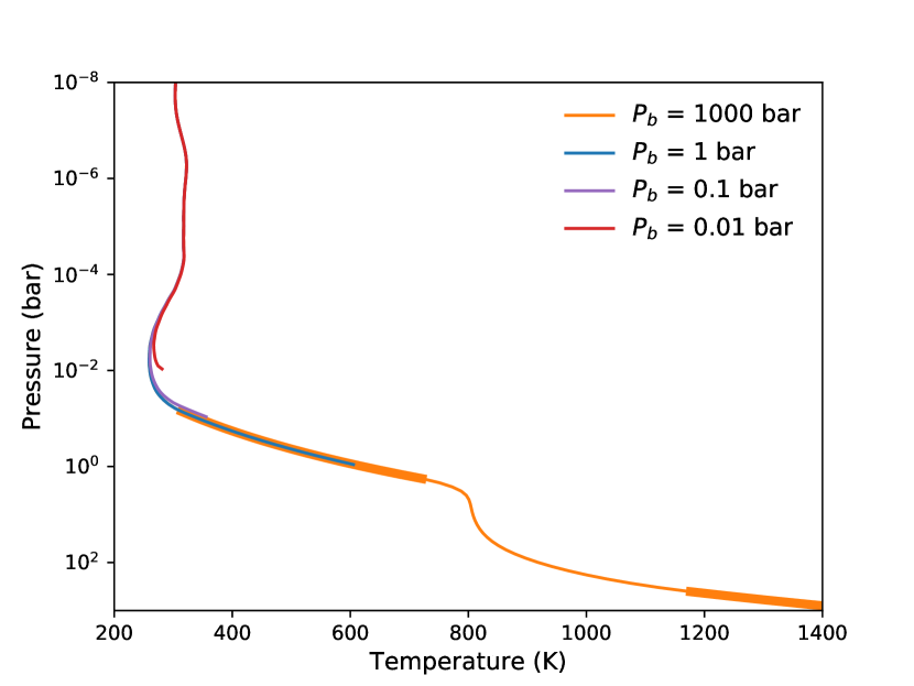
We test the thermal effects of the surface using 1D radiative-convective calculations with a generic surface placed at different pressure levels. We assume a surface albedo of 0.1 but find no differences in the range of 0.1–0.3 (corresponding to the albedo range of land areas on Earth)222Note that we assume a wavelength-independent surface albedo, which likely underestimates the impact of the albedo on the surface temperature.. The resulting temperature profiles for 100 times solar metallicity are depicted in Figure 1. The convective zone extends from a few bar to 0.1 bar and the temperature is set by the dry adiabat. The presence of a surface turns out to have negligible thermal effects in this region since the atmosphere absorbs most of the stellar irradiation. Only for surface pressures around 0.01 bar, the greenhouse warming near the surface starts to be notable, because the atmosphere is optically thin toward stellar radiation while being thermally opaque in this region. In all cases, our test validates the approach of directly truncating the model for shallow atmospheres with surface pressure down to about 1 bar (also see May & Rauscher (2020) for the global heat transport).
3.2 Nitrogen conversion for a quiet M star and an active M star
Photochemically active gases, including \ceNH3, HCN, and \ceCH4, are lost in the absence of a deep atmosphere where themochemistry operates fast and fully recycles them back. Comparing the results of a surface at 1 bar to the deep/no surface case, Yu et al. (2021) find that \ceNH3 is decreased by about 5 orders of magnitude while HCN is decreased by about 3 orders of magnitude. In this section, we will address the timescale of nitrogen conversion and overall compositional evolution driven by photochemistry. It is relevant to consider the host star at different stages when the timescale of chemical destruction is comparable to the timescale of stellar evolution. We apply the synthetic M2 star at the age of 45 Myr and 5 Gyr from HAZMAT (Peacock et al., 2020) for the stellar UV spectra, to represent a young, active and an old, quiet M star333Yu et al. (2021) consider a young, active M star with the UV flux compiled from several stars..
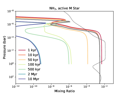
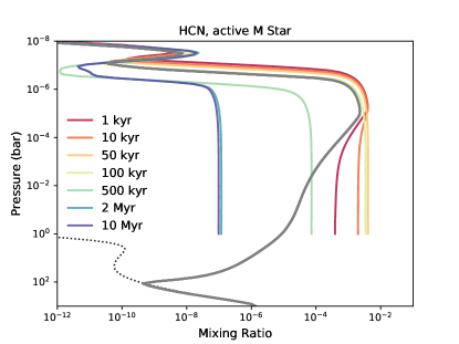
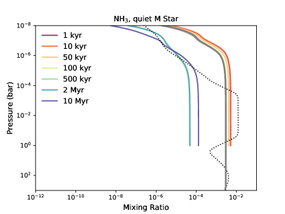
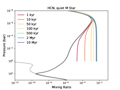
Figure 2 shows snapshots of \ceNH3 and HCN abundances at different times with a 1-bar surface compared with a deep, 1000-bar surface, for both a quiet M star and an active M star444The complete abundance profiles are available in the supplementary materials. All models start from initial abundances in chemical equilibrium. We first confirm that while recycling is enabled in the deep surface scenario, \ceNH3 and HCN settle to a steady state within 1000 years. In the 1-bar atmosphere, \ceNH3 mostly drops off between 10 kyr and 1 Myr to a final mixing ratio several orders of magnitudes lower, qualitatively matching the decrease of \ceNH3 in Yu et al. (2021). However, as \ceNH3 is gradually lost, HCN does not readily follow \ceNH3. With a quiet M star, HCN actually increases to a uniform abundance close to 1 in the period between 0.1 and 10 Myr before gradually declining after 10 Myr.
The timescale of nitrogen conversion given by the evolution of major nitrogen species is further captured in Figure 3 (a). Overall, we find that nitrogen conversion takes place between 10 kyr and 1 Myr for an active M star and is much slower for a quiet M star. \ceNH3 is evidently converted to \ceN2 for an active M star, but HCN can serve as a transient nitrogen pool in the case of a quiet M star.
3.2.1 The two conversion paths of \ceNH3
HCN is produced in the upper atmosphere initiated by \ceNH3 photolysis:
| (3) |
While HCN is subject to photodissociation into cyanide radical (CN) and H, CN can rapidly recycle back to HCN with \ceCN + H2 -¿ HCN + H in an \ceH2 atmosphere. In fact, the major effective sink of HCN is the OH radical produced by water photolysis. HCN is consumed by OH as C irreversibly goes into CO and N converted into \ceN2. The primary scheme for the loss of \ceNH3 and HCN through oxidation is
| (4) |
The critical difference between a quiet and an active M star is that an active M star produces orders-of-magnitude more OH radicals and hence HCN is scavenged more efficiently after building up. On the other hand, HCN is gradually consumed by OH only after 10 Myr with a quiet M star. We can estimate the overall nitrogen conversion timescale of scheme (4) with its rate-limiting step (Tsai et al., 2018)
| (5) |
where is the rate coefficient for the reaction \ceNH2 + NO -¿ N2 + H2O. Taking the initial abundances at 0.1 mbar and 1000 years, the timescale of \ceNH3 by (5) is 0.1 Myr for an active M star and 10 Gyr for a quiet M star, consistent with the kinetics results. This is not to be confused with the timescale of \ceNH3 photodissociation, which operates much faster, about a few hours at the same pressure level.
We conclude this section by reiterating that although the ammonia loss in the shallow-surface case is driven by photochemistry, the process of nitrogen conversion occurs over a timescale of a million years or longer for quiet M stars. It resembles denitrification processes on a geological timescale but only takes place in the atmosphere rather than shifting between reservoirs.
3.3 Carbon conversion
Most of the carbon is initially bound in the photochemically unstable \ceCH4 and converted into CO and \ceCO2 over time. The same evolution of carbon species is shown in Figure 3 (b). First, carbon conversion takes about the same timescale as the nitrogen conversion, (Myr). Second, the conversion of \ceCH4 to CO and \ceCO2 is initiated by the \ceCH4 photodissociation channel: \ceCH4 -¿[hν] CH + H2 + H. CH reacts with \ceH2O to form \ceH2CO, which is readily photodissociated into CO. This conversion proceeds faster with an active M star but the final abundances of CO and \ceCO2 remain close independent of the host star. Third, \ceCH4 is still continuously evolving after millions of years with a quiet M star, making it ambiguous to compare with the deep-atmosphere abundance as a proxy for surface pressure. Last and most interestingly, methanol (\ceCH3OH) is produced as a by-product of carbon conversion. A small part of \ceH2CO, instead of being photodissociated, can thermally react with hydrogen to form \ceCH3O and \ceCH3OH. The mixing ratio of \ceCH3OH is increased to 10-6, compared to 10-9 and 10-8 in the deep surface scenario for a quiet and an active M star, respectively, where \ceCH3OH is transported and destroyed in the deep atmosphere.
3.4 Sensitivity to metallicity
Sub-Neptunes can in general have a wide range of atmospheric metallicity (Moses et al., 2013; Fortney et al., 2013). The equilibrium abundance of \ceNH3 decreases with increasing metallicity as a result of hydrogen deficiency. To test the sensitivity of \ceNH3 conversion to metallicity, we further explore lower metallicities with the same – structure. Figure 3 (c) illustrates the evolution of major nitrogen species for 1, 10, and 100 solar metallicity, with a 1-bar surface and an active M star, where the abundances are normalized to those in equilibrium for a clearer comparison between different metallicities. The final [\ceNH3]/[\ceNH3] slightly decreases with smaller metallicity while [HCN]/[HCN] is almost identical for all metallicities. We find that the trends of \ceNH3 and HCN destruction remain robust. The (Myr) timescale of nitrogen conversion holds across different metallicities as well.
3.5 Sensitivity to vertical mixing
The eddy diffusion profile in our nominal model prescribed by Equation (1) is close to that in Yu et al. (2021). The inverse square root of pressure dependence of is commonly assumed to reflect the turbulent mixing due to gravity wave breaking in stratified atmospheres (e.g., Lindzen, 1981; Moses et al., 2016). Since the eddy diffusion cannot be derived from first principles and is often treated as a free parameter, we further test the sensitivity to the strength and structure of vertical mixing by running the 1-bar surface case for a range of uniform profiles from 105 to 109 cm2/s. This range of eddy diffusion coefficient is consistent with that derived from the average vertical wind in the GCM of K2-18b (see Figure 7) and other sub-Neptunes in a similar dynamical regime (e.g., Charnay et al. (2015)).
The mixing ratios of \ceNH3, HCN, and \ceCH3OH for different assumptions of eddy diffusion coefficient are reported in Figure 3 (d). \ceNH3 in the deep model retains a uniform abundance (Figure 2) and does not depend on the eddy diffusion, whereas \ceNH3 decrease in the shallow model generally correlates with smaller eddy diffusion, since the lower well-mixed region leads to deeper UV penetration and photochemical destruction. Overall, \ceNH3 always has lower abundances in the shallow model than those in the deep model but the exact ratio, [\ceNH3]/[\ceNH3], depends on the strength and shape of . On the other hand, \ceCH3OH consistently shows little sensitivity to eddy diffusion and about two orders of magnitude increase with respect to the deep model. Conversely, HCN highly depends on eddy diffusion as a result of the balance between photochemical production/destruction in the upper atmosphere and vertical transport. HCN can either raise or lower in the presence of a shallow surface, making it unsuitable as a proxy for the surface level.
4 2D Results: Globally Uniform Distribution controlled by the dayside
We have established the long, (Myr) timescale of the nitrogen conversion in Section 3. On a tidally locked exoplanet, the conversion driven by photochemistry only occurs on the dayside but completely shuts down on the permanent nightside. Without photolysis, \ceNH3 is able to maintain a high abundance on the nightside. To answer the question how the chemical evolution with a shallow surface would be regulated by the global circulation between the dayside and nightside, we apply a 2D photochemical model on a meridionally averaged equatorial plane to address the effects of day-night transport.
The temperature and wind for the 2D photochemical model are adopted from the 3D GCM output of K2-18b, whose global structure can be found in Figure 7. We employ four quarters (Figure 7 (d)) in our 2D model for clarity, while the full 2D chemical output is included in the supplementary figure. To isolate the effects of horizontal transport, Figure 4 compares the steady-state abundances with a 1-bar surface and an active M star to those without including the zonal wind.
It is evident that without a recycling mechanism, the horizontal transport is able to exhaust \ceNH3 on the nightside. Even the modest zonal wind ( 1 m/s) yields a horizontal transport timescale less than a year, orders of magnitude faster than the chemical evolution. As a result, most species are homogenized below 1 mbar and exhibit abundances close to those predicted by the 1D model without day-night transport. The model for a quiet M star shows qualitatively consistent results (Figure 6), with reduced photochemical destruction of \ceNH3 and higher abundance of HCN. The results we find for the fiducial example of K2-18b can be generalized to most temperate, tidally-locked planets with a chemically inactive surface, since the equatorial jet is a robust dynamical property (e.g. Pierrehumbert & Hammond, 2019).
5 Spectral Indicator
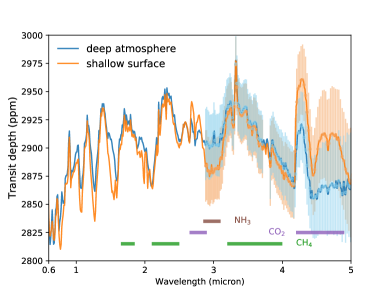
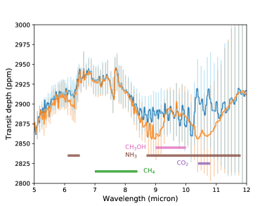
Since the 1D model for the dayside is verified to represent the globally uniform distribution, we compare the transmission spectra from our deep-atmosphere and shallow-surface models in Figure 5. The most distinctive differences are \ceCO2 absorption features at 4.2 – 5 and the lack of \ceNH3 at 3, 8.8 – 12 for the shallow-surface case. Interestingly, \ceCH3OH absorbs between 9 and 10 , well within the \ceNH3 band. To quantify the ability of detecting these molecules with JWST, we used Pandexo (Batalha et al., 2017) to generate the required observations to disentangle between our two models. We find that with it is possible to identify the \ceNH3 feature at 3 with only 3 transit observations using NIRSpec. When observing with MIRI, it is possible to further discriminate \ceCH3OH from \ceNH3 with around 20 transits. Conversely, HCN is not abundant enough in the region sensitive to transmission to show observable features.
6 Discussion
Interactions with the planetary interior are not included in this work as we assume zero flux at the lower (surface) boundary for all species. Regarding \ceNH3, agricultural ammonia on Earth is absorbed by surfaces with a fairly short residence time ( days, e.g., Seinfeld & Pandis, 2016; Jia et al., 2016). We have tested our model with Earth surface conditions assuming biotic processes are involved, and even the slowest dry deposition of \ceNH3 on a desert ( cm/s, Jia et al., 2016) acts as a more efficient sink than the photochemical sink (Section 3). However, without the biosphere transferring ammonia to different organic nitrogen, it is conceivable that ammonia returns to the atmosphere at once and makes effectively net zero deposition. In general, various geological processes can be crucial in controlling trace gases in the atmosphere, especially determining the redox state of the atmosphere. For example, Wogan et al. (2020) find volcanic outgassing unlikely to be reducing, while Lichtenberg (2021) demonstrate that the interior of sub-Neptunes can remain reducing due to vigorous internal convection and Zahnle et al. (2020) suggest iron-rich impacts can also generate reducing atmospheres that favor \ceNH3 and \ceCH4. In the case of an atmosphere with scattering clouds/hazes or less irradiated than K2-18b (Piette & Madhusudhan, 2020; Blain, D. et al., 2021), the surface temperature can be brought down to suppress water evaporation (Scheucher et al., 2020) and allow liquid water oceans, which can participate in regulating the inventory of soluble gases (e.g., \ceNH3, \ceCO2, and \ceCH3OH). With mobile lid tectonics (Tackley et al., 2013; Meier et al., 2021), the long-term evolution of \ceCO2 in the shallow atmosphere case is expected to be governed by outgassing and weathering (e.g. Pierrehumbert, 2010).
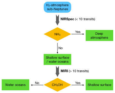
Since \ceCO2 generally has other geological sources and HCN is unsuitable as a surface proxy for its strong dependence on the stellar type and vertical mixing, we propose including \ceCH3OH as a complementary indicator along with \ceNH3. On Earth, \ceCH3OH is mainly produced by plants and deposited to the ocean (Yang et al., 2013), whereas in a \ceH2-dominated atmosphere with a shallow surface, \ceCH3OH is produced during the process of \ceCH4 oxidation. Detection of \ceNH3 without \ceCH3OH is consistent with the deep/no-surface scenario, while detection of \ceCH3OH but without \ceNH3 indicates the presence of a surface. Non-detection of both \ceNH3 and \ceCH3OH can imply a global water-ocean world (Hu et al., 2021) as they are highly soluble in water. We summarize the flowchart of inferring the surface property of sub-Neptunes with \ceH2-dominated atmospheres using JWST in the bottom panel of Figure 5.
7 Summary
1D modeling of sub-Neptune exoplanets suggests that \ceNH3 is depleted below detectable level on the dayside in the presence of a shallow surface, while HCN can either increase or decrease depending on vertical mixing and quiet/active M stars. \ceCH3OH is found to be consistently enhanced for all shallow-surface simulations. We construct a 2D photochemical framework to account for the day-night circulation and find the global abundance is overall quenched from the dayside as the chemical conversion takes (Myr). Our results suggest that HCN is not applicable to determine the pressure level of the surface. Instead, the shallow-surface scenario can be ruled out by \ceNH3 detection, whereas positive detection of \ceCH3OH with negative detection of \ceNH3 indicate shallow and dry surfaces.
acknowledgments
S.-M.T. acknowledges support from the European community through the ERC advanced grant EXOCONDENSE (#740963; PI: R.T. Pierrehumbert). T.L. has been supported by the Simons Foundation (SCOL award #611576). This work has made use of the synthetic spectra from the HAZMAT program; doi:10.17909/t9-j6bz-5g89. We thank J. Moses for thoughtful discussion.
References
- Aguichine et al. (2021) Aguichine, A., Mousis, O., Deleuil, M., & Marcq, E. 2021, ApJ, 914, 84, doi: 10.3847/1538-4357/abfa99
- Agúndez et al. (2014) Agúndez, M., Venot, O., Selsis, F., & Iro, N. 2014, ApJ, 781, 68, doi: 10.1088/0004-637X/781/2/68
- Batalha et al. (2017) Batalha, N. E., Mandell, A., Pontoppidan, K., et al. 2017, PASP, 129, 064501, doi: 10.1088/1538-3873/aa65b0
- Bean et al. (2021) Bean, J. L., Raymond, S. N., & Owen, J. E. 2021, Journal of Geophysical Research (Planets), 126, e06639, doi: 10.1029/2020JE006639
- Benneke et al. (2019) Benneke, B., Wong, I., Piaulet, C., et al. 2019, ApJ, 887, L14, doi: 10.3847/2041-8213/ab59dc
- Blain, D. et al. (2021) Blain, D., Charnay, B., & Bézard, B. 2021, A&A, 646, A15, doi: 10.1051/0004-6361/202039072
- Charnay et al. (2015) Charnay, B., Meadows, V., & Leconte, J. 2015, ApJ, 813, 15, doi: 10.1088/0004-637X/813/1/15
- Chubb et al. (2021) Chubb, K. L., Rocchetto, M., Yurchenko, S. N., et al. 2021, A&A, 646, A21, doi: 10.1051/0004-6361/202038350
- Coles et al. (2019) Coles, P. A., , Yurchenko, S. N., & Tennyson, J. 2019, Mon. Not. R. Astron. Soc., 490, 4638, doi: 10.1093/mnras/stz2778
- Drummond et al. (2020) Drummond, B., Hébrard, E., Mayne, N. J., et al. 2020, A&A, 636, A68, doi: 10.1051/0004-6361/201937153
- Feng et al. (2020) Feng, Y. K., Line, M. R., & Fortney, J. J. 2020, The Astronomical Journal, 160, 137, doi: 10.3847/1538-3881/aba8f9
- Fortney et al. (2013) Fortney, J. J., Mordasini, C., Nettelmann, N., et al. 2013, ApJ, 775, 80, doi: 10.1088/0004-637X/775/1/80
- Gordon & et al. (2017) Gordon, I. E., & et al. 2017, J. Quant. Spectrosc. Radiat. Transf., 203, 3, doi: 10.1016/j.jqsrt.2017.06.038
- Hammond & Pierrehumbert (2017) Hammond, M., & Pierrehumbert, R. T. 2017, The Astrophysical Journal, 849, 152, doi: 10.3847/1538-4357/aa9328
- Hammond & Pierrehumbert (2018) Hammond, M., & Pierrehumbert, R. T. 2018, The Astrophysical Journal, 869, 65, doi: 10.3847/1538-4357/aaec03
- Hsu et al. (2019) Hsu, D. C., Ford, E. B., Ragozzine, D., & Ashby, K. 2019, AJ, 158, 109, doi: 10.3847/1538-3881/ab31ab
- Hu et al. (2021) Hu, R., Damiano, M., Scheucher, M., et al. 2021, 921, L8, doi: 10.3847/2041-8213/ac1f92
- Hunter (2007) Hunter, J. D. 2007, Computing in Science Engineering, 9, 90, doi: 10.1109/MCSE.2007.55
- Irwin et al. (2008) Irwin, P. G. J., Teanby, N. A., de Kok, R., et al. 2008, J. Quant. Spec. Radiat. Transf., 109, 1136, doi: 10.1016/j.jqsrt.2007.11.006
- Jia et al. (2016) Jia, Y., Yu, G., Gao, Y., et al. 2016, Scientific Reports, 6, 19810, doi: 10.1038/srep19810
- Lee et al. (2021) Lee, E. K. H., Parmentier, V., Hammond, M., et al. 2021, MNRAS, 000, 1. https://arxiv.org/abs/2106.11664
- Lee et al. (2020) Lee, G. K., Casewell, S. L., Chubb, K. L., et al. 2020, Monthly Notices of the Royal Astronomical Society, 496, 4674, doi: 10.1093/mnras/staa1882
- Li et al. (2015) Li, G., Gordon, I. E., Rothman, L. S., et al. 2015, Astrophys. J. Suppl., 216, 15, doi: 10.1088/0067-0049/216/1/15
- Lichtenberg (2021) Lichtenberg, T. 2021, ApJ, 914, L4, doi: 10.3847/2041-8213/ac0146
- Lindzen (1981) Lindzen, R. S. 1981, Journal of Geophysical Research: Oceans, 86, 9707, doi: https://doi.org/10.1029/JC086iC10p09707
- Lopez & Fortney (2013) Lopez, E. D., & Fortney, J. J. 2013, The Astrophysical Journal, 776, 2, doi: 10.1088/0004-637x/776/1/2
- Madhusudhan et al. (2020) Madhusudhan, N., Nixon, M. C., Welbanks, L., Piette, A. A. A., & Booth, R. A. 2020, ApJ, 891, L7, doi: 10.3847/2041-8213/ab7229
- Malik et al. (2019b) Malik, M., Kempton, E. M. R., Koll, D. D. B., et al. 2019b, ApJ, 886, 142, doi: 10.3847/1538-4357/ab4a05
- Malik et al. (2019a) Malik, M., Kitzmann, D., Mendonça, J. M., et al. 2019a, The Astronomical Journal, 157, 170, doi: 10.3847/1538-3881/ab1084
- May & Rauscher (2020) May, E. M., & Rauscher, E. 2020, ApJ, 893, 161, doi: 10.3847/1538-4357/ab838b
- Meier et al. (2021) Meier, T. G., Bower, D. J., Lichtenberg, T., Tackley, P. J., & Demory, B.-O. 2021, ApJ, 908, L48, doi: 10.3847/2041-8213/abe400
- Moses et al. (2013) Moses, J. I., Line, M. R., Visscher, C., et al. 2013, The Astrophysical Journal, 777, 34, doi: 10.1088/0004-637x/777/1/34
- Moses et al. (2016) Moses, J. I., Marley, M. S., Zahnle, K., et al. 2016, The Astrophysical Journal, 829, 66, doi: 10.3847/0004-637x/829/2/66
- Oliphant (2007) Oliphant, T. E. 2007, Computing in Science Engineering, 9, 10, doi: 10.1109/MCSE.2007.58
- Peacock et al. (2020) Peacock, S., Barman, T., Shkolnik, E. L., et al. 2020, ApJ, 895, 5, doi: 10.3847/1538-4357/ab893a
- Pierrehumbert (2010) Pierrehumbert, R. T. 2010, Principles of Planetary Climate
- Pierrehumbert & Ding (2016) Pierrehumbert, R. T., & Ding, F. 2016, Proceedings of the Royal Society A: Mathematical, Physical and Engineering Sciences, 472, doi: 10.1098/rspa.2016.0107
- Pierrehumbert & Hammond (2019) Pierrehumbert, R. T., & Hammond, M. 2019, Annual Review of Fluid Mechanics, 51, 275, doi: 10.1146/annurev-fluid-010518-040516
- Piette & Madhusudhan (2020) Piette, A. A. A., & Madhusudhan, N. 2020, ApJ, 904, 154, doi: 10.3847/1538-4357/abbfb1
- Scheucher et al. (2020) Scheucher, M., Wunderlich, F., Grenfell, J. L., et al. 2020, 898, 44, doi: 10.3847/1538-4357/ab9084
- Seinfeld & Pandis (2016) Seinfeld, J. H., & Pandis, S. N. 2016, Atmospheric chemistry and physics: from air pollution to climate change (John Wiley & Sons, Inc.)
- Tackley et al. (2013) Tackley, P. J., Ammann, M., Brodholt, J. P., Dobson, D. P., & Valencia, D. 2013, Icarus, 225, 50, doi: 10.1016/j.icarus.2013.03.013
- Tsai et al. (2018) Tsai, S.-M., Kitzmann, D., Lyons, J. R., et al. 2018, ApJ, 862, 31, doi: 10.3847/1538-4357/aac834
- Tsai et al. (2017) Tsai, S.-M., Lyons, J. R., Grosheintz, L., et al. 2017, Astrophys. J. Suppl. Ser., 228, 1, doi: 10.3847/1538-4365/228/2/20
- Tsai et al. (2021) Tsai, S.-M., Malik, M., Kitzmann, D., et al. 2021, arXiv e-prints, arXiv:2108.01790. https://arxiv.org/abs/2108.01790
- Tsiaras et al. (2019) Tsiaras, A., Waldmann, I. P., Tinetti, G., Tennyson, J., & Yurchenko, S. N. 2019, Nature Astronomy, 3, 1086, doi: 10.1038/s41550-019-0878-9
- van der Walt et al. (2011) van der Walt, S., Colbert, S. C., & Varoquaux, G. 2011, Computing in Science Engineering, 13, 22, doi: 10.1109/MCSE.2011.37
- Wardenier et al. (2021) Wardenier, J. P., Parmentier, V., Lee, E. K. H., Line, M. R., & Gharib-Nezhad, E. 2021, MNRAS, 506, 1258, doi: 10.1093/mnras/stab1797
- Wogan et al. (2020) Wogan, N., Krissansen-Totton, J., & Catling, D. C. 2020, The Planetary Science Journal, 1, 58, doi: 10.3847/psj/abb99e
- Yang et al. (2013) Yang, M., Nightingale, P. D., Beale, R., et al. 2013, Proceedings of the National Academy of Science, 110, 20034, doi: 10.1073/pnas.1317840110
- Yu et al. (2021) Yu, X., Moses, J. I., Fortney, J. J., & Zhang, X. 2021, ApJ, 914, 38, doi: 10.3847/1538-4357/abfdc7
- Yurchenko et al. (2020) Yurchenko, S. N., Mellor, T. M., Freedman, R. S., & Tennyson, J. 2020, Mon. Not. R. Astron. Soc., 496, 5282, doi: 10.1093/mnras/staa1874
- Zahnle et al. (2020) Zahnle, K. J., Lupu, R., Catling, D. C., & Wogan, N. 2020, The Planetary Science Journal, 1, 11, doi: 10.3847/psj/ab7e2c
- Zilinskas et al. (2020) Zilinskas, M., Miguel, Y., Mollière, P., & Tsai, S.-M. 2020, MNRAS, 494, 1490, doi: 10.1093/mnras/staa724
Appendix A Radiative feedback from disequilibrium chemistry
Since the temperature structure is fixed by thermochemical equilibrium, we have also checked the radiative feedback as a result of disequilibrium chemistry. We re-run the 1D radiative-convective calculations with the final disequilibrium composition from Section 3. We find the resulting temperature from disequilibrium chemistry can be about 100 K lower at most in the convective zone above 1 bar, mainly from the decrease of opacity-predominating water. We have performed sensitivity tests and found the temperature difference does not alter the presented results (also see the thermal structure variance explored in Yu et al. (2021)). We will leave the effects of water condensation for future work.
Appendix B Running 2D photochemical models for millions years
The horizontal transport flux by the zonal wind in Equation (2) yields a hyperbolic partial differential equation. The time step is ought to follow the same format as Courant–Friedrichs–Lewy (CFL) condition when numerically integrating the system. In other words, the time step must not exceed the time that zonal flow travels across adjacent vertical columns. For K2-18b, the time step limit is s, which means more than integration steps are required to integrate the system to a million year for the long-term chemical evolution. To circumvent this computational load, we arbitrarily slow down the zonal wind (e.g., by 1000 times) such that a larger time step can be adopted. Once the chemistry has evolved after the Myr integration, we recover the correct wind velocity and run the model to final steady state. This seemingly risky approach can be justified by the timescale argument: The horizontal transport effectively interacts with vertical mixing and chemical evolution , which manifest drastically different timescales. The timescale of vertical mixing is within hours and the chemical evolution takes Myr, whereas the nominal horizontal transport has a timescale of days. Therefore, the long-term compositional evolution is expected to be qualitatively unaffected for any horizontal transport much slower than vertical mixing but orders of magnitude faster than the chemical evolution. That is, the tuned-down zonal wind still plays the role of passing on the chemical evolution from dayside to nightside. Finally, we have confirmed this approach by comparing the simulation at about 5000 years to that with 1000 times slower zonal wind and found no differences.