Quantum Information Dimension and Geometric Entropy

Abstract

Geometric quantum mechanics, through its differential-geometric underpinning, provides additional tools of analysis and interpretation that bring quantum mechanics closer to classical mechanics: state spaces in both are equipped with symplectic geometry. This opens the door to revisiting foundational questions and issues, such as the nature of quantum entropy, from a geometric perspective. Central to this is the concept of geometric quantum state—the probability measure on a system’s space of pure states. This space’s continuity leads us to introduce two analysis tools, inspired by Renyi’s information theory, to characterize and quantify fundamental properties of geometric quantum states: the quantum information dimension that is the rate of geometric quantum state compression and the dimensional geometric entropy that monitors information stored in quantum states. We recount their classical definitions, information-theoretic meanings, and physical interpretations, and adapt them to quantum systems via the geometric approach. We then explicitly compute them in various examples and classes of quantum system. We conclude commenting on future directions for information in geometric quantum mechanics.

I Introduction

When connecting theory to experiment both classical and quantum mechanics (CM and QM) must cope with the emergence of randomness and uncertainty. However, the nature of randomness differs. While inherent in QM (Born’s rule), in CM it dynamically emerges via the instabilities associated with deterministic chaos. In CM, dynamical systems theory provides the correct set of tools to model and explain the emergent stochastic dynamics of both Hamiltonian and dissipative systems. Building on previous results [1] that leverage the geometric parallels between classical and quantum state spaces (both symplectic manifolds), in this manuscript we extend several tools of analysis for the out-of-equilibrium phenomena of classical systems to the quantum domain. This strengthens the parallels and provides a novel paradigm for investigating open quantum systems out of equilibrium. More specifically, following Kolmogorov and Sinai’s use of Shannon’s information theory [2] to quantify degrees of deterministic chaos [3, 4, 5, 6, 7, 8], we show that the parallels go even deeper and lead to new descriptive and quantitative tools. This is done by leveraging Geometric Quantum Mechanics, an approach to quantum mechanics based on differential geometry which gets rid of the physical redundancies intrinsic to the standard, linear algebra, approach.

Quantum mechanics, indeed, is grounded in a formalism in which the states of a discrete system are vectors in a complex Hilbert space $\mathcal{H}$ of generic finite dimension $D$. However, it is well-known that such a formulation is redundant since vectors differing only in normalization and global phase are physically equivalent. Implementing this equivalence relation leads to the space where quantum states live: the complex projective Hilbert space $\mathcal{P}(\mathcal{H})\sim\mathbb{C}P^{D-1}$. This is the starting point for a differential-geometric formulation of quantum mechanics called geometric quantum mechanics [9, 10, 11, 12, 13, 14, 15, 16, 17, 18, 19, 20, 21, 22, 23, 24, 25, 26]. It is important to stress that, while the mathematical formulation differs, the phenomena addressed are precisely the same as standard quantum mechanics.

Geometric quantum mechanics (GQM) works with probability densities on $\mathcal{P}(\mathcal{H})$. These are interpreted using ensemble theory, as noninteracting copies of pure states for the same quantum system, distributed according to some measure. This leads to the concept of—geometric quantum state (GQS)—as an ensemble of pure states. (For an extensive analysis we recommend Ref. [18].) This is a more fundamental notion of quantum state than the density matrix, as the latter can be computed from the former, but not vice versa.

Recent work provided a concrete procedure to analytically compute the GQS of an open, finite-dimensional, quantum system interacting with another one of arbitrary dimension (both finite and infinite) [1]. This revealed the reason why the GQS provides a more accurate description than available with a density matrix: The GQS retains the details about how a specific ensemble of pure states emerges from the structure of correlations between the system and its surroundings.

Starting from this foundation, the following introduces two information-theoretic concepts to characterize geometric quantum states. The first is the quantum information dimension. This borrows from Renyi’s notion of the effective dimension of a continuous probability distribution, developed in the setting of efficiently transmitting continuous variables over noisy communication channels. Interestingly, for classical variables there are distributions for which the dimension is not an integer—the realizations of these are the well-known fractals [27]. It also has an operational interpretation within communication theory: it is the upper bound on the lossless compression rate for transmitting GQSs. The second GQS characterization uses the (related) concept of dimensional geometric entropy. Accounting for GQS dimension, this entropy quantifies the information a GQS stores about a quantum system.

The development unfolds as follows. Section II gives a brief summary of geometric quantum mechanics and the notion of geometric quantum state. Section III defines the quantum information dimension, while Section IV introduces the dimensional geometric entropy. Sections V.1 to V.4 then analyze several examples, evaluating these quantities exactly. The first is an open quantum system interacting with a finite-dimensional environment. The second is an open quantum system interacting with another with an infinite-dimensional Hilbert space (continuous degrees of freedom). The third shows how to evaluate these quantities in a discrete-time chaotic quantum dynamics. The fourth shows how to evaluate these quantities in the thermodynamic limit for a condensed-matter system in its ground state. Finally, Section VI discusses the results and Section VII draws forward-looking conclusions.

II Geometric Quantum Mechanics

References [9, 10, 11, 12, 13, 14, 15, 16, 17, 18, 19, 20, 21, 22, 23, 24, 25, 26] lay out the mathematical physics of geometric quantum mechanics. Here, we simply recall the aspects most relevant for our purposes. Throughout, we only address quantum systems with a Hilbert space $\mathcal{H}$ of finite dimension $D$. In GQM, the pure states of such systems are points $Z$ in the complex projective space $\mathcal{P}(\mathcal{H})\sim\mathbb{C}P^{D-1}$. Given an arbitrary basis $\left\{\ket{b_{\alpha}}\right\}_{\alpha}$ of $\mathcal{H}$, the pure state $Z$ has the vector representation:

$$\ket{Z}\coloneqq\sum_{\alpha=0}^{D-1}Z_{\alpha}\ket{b_{\alpha}}\leavevmode\nobreak\ ,$$

where $Z_{\alpha}\in\mathbb{C}$ and $Z\sim\lambda Z$, with $\lambda\in\mathbb{C}$. This space has a rich geometric structure [28]. In particular, there is a well-defined metric—the Fubini-Study metric $g_{FS}$—and a related notion of Volume $dV_{FS}$—the Fubini-Study volume element. These are directly connected by $dV_{FS}=\sqrt{\det g_{FS}}dZd\overline{Z}$, where the overbar is the complex conjugate and $dZ$ is the Lebesgue measure. While a full explication is beyond our current scope, we simply give its explicit form in a particular coordinate system, specified by $Z_{\alpha}=\sqrt{p_{\alpha}}e^{i\phi_{\alpha}}$: $dV_{FS}=\prod_{\alpha=1}^{D-1}\left(dp_{\alpha}d\phi_{\alpha}/2\right)$.

On $\mathcal{P}(\mathcal{H})$, one considers ensembles distributed according to a probability density function or, more generally, a probability measure $\mu$. The simplest example is the basic definition of the uniform measure: $d\nu_{FS}\coloneqq dV_{FS}/V_{D-1}$, where the total Fubini-Study volume of $\mathcal{P}(\mathcal{H})$ is $V_{D-1}=\pi^{D-1}/(D-1)!$. This determines the basic notion of uniform measure on $\mathcal{P}(\mathcal{H})$. Calling $A$ an element of $\mathcal{P}(\mathcal{H})$’s Borel $\sigma$-algebra and adopting the De Finetti notation, we have:

$$\nu_{FS}(A)=\frac{1}{V_{D-1}}\int_{A}dV_{FS}\leavevmode\nobreak\ .$$

In general cases, the measure $\mu$ is not uniform and one has:

$$\mu(A)=\int_{A}\mu(d\nu_{FS})\leavevmode\nobreak\ .$$

Looking at the measure-theoretic definition, if $\mu$ is absolutely continuous with respect to $\nu_{FS}$, then there is a probability density function $q(Z=z)$ such that:

$$\mu_{q}(A)=\int_{A}q(z)d\nu_{FS}\leavevmode\nobreak\ .$$

This is interpreted by saying that $\mu_{q}(d\nu_{FS}^{z})=q(z)d\nu_{FS}^{z}$ is the infinitesimal probability of a realization $z$—i.e., a system pure state—belonging to an infinitesimal volume $d\nu_{FS}^{z}$ centered at $z\in\mathcal{P}(\mathcal{H})$. Thus, we can think about the pure state of a quantum system as a realization $z$ of a random variable $Z$ with sample space $\mathcal{P}(\mathcal{H})$. Here, $z$ is distributed on $\mathcal{P}(\mathcal{H})$ according to its geometric quantum state $q(z)$ or $\mu$. Through an abuse of language, we often refer to both the measure $\mu$ and the density $q$ (when it exists) as geometric quantum states. This is acceptable as they convey the same kind of information.

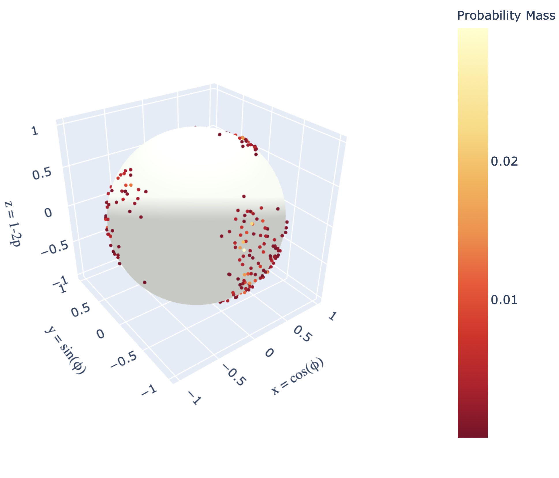
Figure 1: Geometric quantum state $q(Z)=\sum_{k=1}^{2^{9}}p_{k}\delta[Z-Z_{k}]$ on $\mathbb{C}P^{1}$, with coordinates $(\theta,\phi)$. It is a finite sum of $2^{9}$ Dirac measures. Each point is a possible pure state $\ket{\psi(Z_{k})}=\cos\theta_{k}/2\ket{0}+\sin\theta_{k}/2e^{i\phi_{k}}\ket{1}$ in which the system can be, with probability $p_{k}$. The specific value of each $p_{k}$ is encoded in a point’s color; see legend.

Together, the triple $(\mathcal{P}(\mathcal{H}),Z,\mu)$ defines a random variable, in the classical sense, in which the sample space is continuous and encodes the underlying quantumness of the physical system we aim to describe. We call this a random quantum variable (RQV). Following standard notation, if $Z$ is an RQV, we denote a realization with a lowercase corresponding letter $z_{j}$. (This is not to be confused with the notation $Z_{\alpha}$, with a Greek label, that refers to the $\alpha$-th component of the vector $\ket{Z}\in\mathcal{H}$.

To aid intuition, Fig. 1 displays an example of geometric quantum states of a qubit, using the $(\theta,\phi)$ coordinates to represent $\mathcal{P}(\mathcal{H})$ as the familiar Bloch sphere.

III Quantum Information Dimension

One GQM advantage we exploit is that it allows the use of classical measure theory and this greatly facilitates modeling of quantum behavior. The price paid is working with an underlying manifold of nontrivial geometry, as just noted. Intuitively, in this way GQM directly encodes “quantumness” in the underlying sampling space’s geometry. Building on this, we now formalize the dimension of a geometric quantum state, extending Renyi’s information theory [29] to the quantum domain.

Given $\mathcal{P}(\mathcal{H})$ and a measure $\mu$ on it, we uniformly discretize the manifold and coarse-grain $\mu$ to obtain a discrete distribution. This is accomplished as follows, using “probabilities + phases” coordinates: $Z_{\alpha}=\sqrt{p_{\alpha}}e^{i\phi_{\alpha}}$. In this, $\left\{p_{\alpha}\right\}_{\alpha=0}^{D-1}$ lives in a probability simplex $\Delta_{D}$, while the phase coordinates $\left\{\phi_{\alpha}\right\}_{\alpha=1}^{D-1}$ live on a $(D-1)$-dimensional torus $\mathbb{T}^{D-1}$.

Given this coordinate set, we directly partition both $\Delta_{D}$ and $\mathbb{T}_{D-1}$ separately, still in a uniform fashion. More accurately, this is a partitioning of the $\sigma$-algebra on $\mathcal{P}(\mathcal{H})$ into a finite and discrete collection of sets. Since both $\Delta_{D}$ and $\mathbb{T}_{D-1}$ are manifolds of real dimension $D-1$, this generates a uniform partition $\left\{Q(\vec{j},\vec{k})\right\}_{\vec{j},\vec{k}}$ of $\mathcal{P}(\mathcal{H})$ with a total number of $L^{D-1}\times L^{D-1}$ cells. This means $\bigcup_{j_{1},\ldots,j_{D-1}=1}^{L}\bigcup_{k_{1},\ldots,k_{D-1}=1}^{L}Q(\vec{j},\vec{k})=\mathcal{P}(\mathcal{H})$, with $Q(\vec{j},\vec{k})\cap Q(\vec{i},\vec{m})=\delta_{\vec{j},\vec{i}}\delta_{\vec{k},\vec{m}}Q(\vec{i},\vec{m})$. Here, $\vec{j}=(j_{1},\ldots,j_{D-1})$ is the multi-index label that runs over the discretization $\left\{\Delta_{D}(\vec{j})\right\}_{\vec{j}}$ of $\Delta_{D}$, with $j_{\alpha}=1,\ldots,L$ and $\vec{k}=(k_{1},\ldots,k_{D-1})$ is the multi-index label that runs over the discretization $\left\{\mathbb{T}_{D-1}(\vec{k})\right\}_{\vec{k}}$ of $\mathbb{T}_{D-1}$, with $k_{\alpha}=1,\ldots,L$.

The reason to partition $\mathcal{P}(\mathcal{H})$ using this coordinate system is the resulting factorization of $d\nu_{FS}$ in “$dp\times d\phi$”:

$$d\nu_{FS}=dP(\Delta_{D})dQ(\mathbb{T}_{D-1})$$

where $dP(\Delta_{D})=(D-1)!\delta\left(\sum_{\alpha=0}^{D-1}p_{\alpha}-1\right)dp_{0}\ldots dp_{D-1}$ is the flat measure on $\Delta_{D}$ and $dQ(\mathbb{T}_{D-1})$ is the flat measure on $\mathbb{T}_{D-1}$.

This allows us to separately discretize the probability simplex and the high-dimensional torus, while also resulting in cells $Q(\vec{j},\vec{k})$ with uniform Fubini-Study volume:

$$V_{D-1}(\epsilon) \coloneqq\nu_{FS}(Q(\vec{j},\vec{k}))$$

$$=\frac{1}{L^{2(D-1)}}$$

$$=\epsilon^{-2(D-1)}\leavevmode\nobreak\ ,$$ (1)

where $\epsilon$ sets the scale of the partition elements. Note that, despite the discretization’s specific coordinate system, the value of $V_{D-1}(\epsilon)$ does not depend on the coordinate system used to do the computation, thanks to the invariance of $d\nu_{FS}$. Therefore, $\left\{Q(\vec{j},\vec{k})\right\}_{\vec{j},\vec{k}}$ defines a good uniform partition of $\mathcal{P}(\mathcal{H})$.

Calling $z_{\vec{j},\vec{k}}$ a generic point in $Q(\vec{j},\vec{k})$, we can now perform the coarse-graining procedure to get a discrete random variable $Z^{\epsilon}$, for $Z\in\mathbb{C}P^{D-1}$:

$$Z\in Q(\vec{j},\vec{k})\quad\Rightarrow\quad Z^{\epsilon}=z_{\vec{j},\vec{k}}\leavevmode\nobreak\ .$$

The probability $p_{\vec{j},\vec{k}}$ of $Z^{\epsilon}\in Q(\vec{j},\vec{k})$ is defined via the coarse-graining procedure:

$$\mathrm{Pr}\left(Z\in Q(\vec{j},\vec{k})\right) =\mu_{q}(Q(\vec{j},\vec{k}))$$

$$=p_{\vec{j},\vec{k}}$$

$$=q(z_{\vec{j},\vec{k}})V_{D-1}(\epsilon)\leavevmode\nobreak\ ,$$ (2)

where (only) in the last equality we assumed the existence of a density $q(Z)$ and, in that case, $z_{\vec{j},\vec{k}}$ is a point inside $Q(\vec{j},\vec{k})$ defined implicitly by $q(z_{\vec{j},\vec{k}})=\mu_{q}(Q(\vec{j},\vec{k}))/V_{D-1}(\epsilon)$. For explorations in discretizing continuous random variables see the lectures in Ref. [30] and relevant developments in Refs. [31, 32].

Given that $Z^{\epsilon}$ is a discrete random variable, we can now use Shannon’s discrete functional to evaluate its entropy:

$$H\left(Z^{\epsilon}\right)=-\sum_{\vec{j},\vec{k}}p_{\vec{j},\vec{k}}\log p_{\vec{j},\vec{k}}\leavevmode\nobreak\ .$$ (3)

Substituting Eq. (1) into Eq. (2) and calling $\mathfrak{D}$ the real dimension of the submanifold of $\mathcal{P}(\mathcal{H})$ on which $q$ has support, then as $\epsilon\to 0$ one has that $H(Z^{\epsilon})$ is linear in $-\log\epsilon$ [29]:

$$H(Z^{\epsilon})\sim_{\epsilon\to 0}-\mathfrak{D}\log\epsilon+\mathfrak{h}\leavevmode\nobreak\ .$$

Note that $q$ can also have support on the whole manifold, in which case $\mathfrak{D}=2(D-1)$—the real dimension of $\mathcal{P}(\mathcal{H})$. Thus, $\mathfrak{D}$’s value in this scaling is the information dimension while, as we show shortly, the offset $\mathfrak{H}$ provides a workable definition of differential entropy for the density $q$ that accounts for the dimension of $q$’s support.

With this in mind, we are now ready to define a geometric quantum state’s quantum information dimension.

Definition 1 (Quantum Information Dimension).

Given a finite-dimensional quantum system with state space $\mathbb{C}P^{D-1}$ and geometric quantum state $q$, the latter’s quantum information dimension $\mathfrak{D}$ is:

$$\mathfrak{D}\coloneqq\lim_{\epsilon\to 0}\frac{H\left(Z^{\epsilon}\right)}{-\log\epsilon}\leavevmode\nobreak\ .$$ (4)

While alternative definitions are possible, see Ref. [33] and references therein, they all aim to rigorously grounding the same idea. And, the alternatives often provide identical values, assuming the validity of some regularity conditions. The key point is that the essence and the result of the development do not change under these alternatives. For a detailed explication of information dimension see Refs. [29, 33, 34].

Note that there are useful theorems for explicitly calculating the information dimension. We use these in the upcoming sections on example quantum systems. Before proceeding to the geometric dimensional quantum entropy, though, we briefly discuss a connection between $\mathfrak{D}$ and analog information theory, where $\mathfrak{D}$’s classical counterpart has a direct interpretation.

Information theoretic underpinning of $\mathfrak{D}$

Quantum information theory takes inspiration from the information theory of classical discrete sources. However, it is well known that quantum states need real numbers to be faithfully represented. In fact, they require several complex numbers or, equivalently, elements of $\mathbb{R}^{2n}$. So, an approach inspired by information theory is appropriate [35] if we can identify a natural extension to situations where the random variables at hand have a continuous sample space. As such, one can also appeal to analog or continuous information theory. An example, relevant for our purposes, of a result from analog information theory is the quasi-lossless compression theorem. Loosely speaking, this answers the question “How much can we compress the information emitted by a continuous source, using continuous variables?”

Rather than giving the full result—for which see Ref. [33]—we simply discuss the essential point. Consider a continuous source emitting realizations $\vec{x}\in\mathcal{X}$ of a random variable $X$. We desire to compress its information. The dimension of $\mathcal{X}$ is arbitrary, but we assume $\mathcal{X}\subseteq\mathbb{R}^{n}$, for some $n$.

Compression can be achieved using $(N,K)$-codes—a pair of encoder-decoder functions. The encoder function $f:\mathcal{X}^{N}\to\mathcal{Y}^{K}$ converts the continuous message into appropriate discrete symbols, belonging to the space $\mathcal{Y}$. The decoder function $g:\mathcal{Y}^{K}\to\mathcal{X}^{N}$ performs the inverse.

Take the probability of making an error as $\delta=\mathrm{Pr}\left[g(f(\vec{x}))\neq\vec{x}\right]$. Call $R(\epsilon)$ the infimum of $R\geq 0$ such that the $\left(N,\lfloor RN\rfloor\right)$ code has $\delta\leq\epsilon$ error. Assuming a linear form for the encoder and decoder, one establishes that there is a fundamental limit to the amount of quasi-lossless (up to $\epsilon$) compression one can reach. This limit is achievable and it is given by the source’s classical information dimension: $R(\epsilon)\leq\mathfrak{D}(X)$.

Here, with a slight abuse of notation, we use the same symbol $\mathfrak{D}$ to also identify the classical information dimension. We also stress that this is only a brief and simplified summary of the comprehensive analysis performed in Ref. [33]. What is relevant for our purposes is the fact that, despite its simplicity, it is directly applicable to quantum systems. In particular, it addresses encoding a quantum source emitting pure states $Z\in\mathbb{C}P^{D-1}$ with a classical continuous distribution given by the geometric quantum state $q$. Moreover, as quantum states themselves are points on a manifold described by continuous variables, it can also be applied to the inverse problem of representing a continuous classical source with quantum states. While this begs further exploration before making rigorous statements, we believe it hints at the fact that there is an alternative way, inspired by analog information theory, of conceptualizing quantum computing.

Before finally moving to dimensional quantum entropy, we highlight a point about $\mathfrak{D}$. While the understanding based on encoding and communication theory strengthens the argument for relevance, $\mathfrak{D}$’s general role in investigating properties of geometric quantum states stands on its own, as it is independently and rigorously defined.

IV Dimensional Quantum Entropy

For a given geometric quantum state, quantum information dimension gives a notion of effective dimension. It is therefore natural that its value affects the definition of entropy one assigns to a geometric quantum state.

The standard example comes from comparing discrete and continuous probability distributions. In the discrete setting there is a unique entropy definition, given by Shannon’s functional:

$$H_{\mathrm{discrete}}=-\sum_{i}p_{i}\log p_{i}\leavevmode\nobreak\ .$$ (5)

Its extension to the continuous domain, however, is not unique and its development and use requires care.

On the one hand, Shannon’s original definition of differential entropy for a continuous variable $X$ with probability distribution $p(x)$ provides a meaningful and interpretable quantity [2]:

$$H_{\mathrm{continuous}}=-\int p(x)\log p(x)dx\leavevmode\nobreak\ .$$ (6)

On the other, it is well known that it presents its own challenges and that alternatives are possible. For example, it is well-known to be sensitive to rescaling of the measure. When $dx\to kdx$ we have that $H_{\mathrm{continuous}}\to H_{\mathrm{continuous}}+\log k$.

Thus, when a physical measure is defined up to an overall scale factor, this quantity is defined up to an overall additive factor. This is an issue that can often be disregarded as it does not carry physical consequences, in analogy with the classical notion of energy, defined up to a constant. Practically, this can be bypassed by fixing the zero point of the entropy to be given by the uniform distribution, which is realized by using as measure the normalized volume of the space so that a uniform density simply has constant value equal to $1$, giving a differential entropy $H_{unif}=\log 1=0$.

Note, too, that $H_{\mathrm{continuous}}$ can be negative, as $-\log p(x)$ can be negative when $p(x)$ is a density. This is not a concern, since correctly interpreting this quantity relies on the asymptotic equipartition property, which holds for both discrete and continuous random variables, irrespective of $H_{\mathrm{continuous}}$’s sign; see Ch. 8 of Ref. [35].

Moreover and finally, the differential entropy is appropriate only when the distribution has integer topological dimension. This is not true, for example, in nonlinear dynamics, in which time-asymptotic statistical states often live on fractals due, for example, to chaotic behavior. These objects do not have integer dimension. However, it is possible to define an entropy that takes this rich phenomenology into account. Again, for the classical result we point to Refs. [29, 33]. Here, we extend this into the quantum domain as follows.

Definition 2 (Dimensional quantum entropy).

Given a finite-dimensional quantum system with state space $\mathbb{C}P^{D-1}$, geometric quantum state $q$ with quantum information dimension $\mathfrak{D}$, we define $q$’s dimensional quantum entropy $H_{\mathfrak{D}}\left[q\right]$ as:

$$H_{\mathfrak{D}}\left[q\right]\coloneqq\lim_{\epsilon\to 0}\big{(}H\left(Z^{\epsilon}\right)+\mathfrak{D}\log\epsilon\big{)}\leavevmode\nobreak\ .$$ (7)

Note that this entropy is parametrized by the quantum information dimension. To provide intuition, consider two simple cases. Shortly after, Secs. V.1 to V.4 present detailed example calculations.

First, assuming that $\mathfrak{D}=0$, we see that $H_{0}\left[Z\right]$ is simply the continuum limit of $Z^{\epsilon}$’s entropy $H(Z^{\epsilon})$. Second, imagine we are looking at the uniform distribution over Bloch sphere $\mathbb{C}P^{1}$. As this is an absolutely continuous distribution, it has quantum information dimension $\mathfrak{D}=2$ and, therefore, the appropriate notion of entropy should take that into account.

We also find that when $\mathfrak{D}=2(D-1)$, $H_{\mathfrak{D}=2(D-1)}[Z]$ is equal to the notion of geometric quantum entropy introduced, as far as we know, by Brody and Hughston in [36] and discussed in Refs. [18, 1, 37, 38]. In the simple case of a qubit with continuous geometric quantum state $q(Z)$ this is:

$$H_{2}\left[Z\right] =\lim_{\epsilon\to 0}\left(H(Z^{\epsilon})+2\log\epsilon\right)$$

$$=-\int_{\mathbb{C}P^{1}}\!\!\!d\nu_{FS}^{Z}q(Z)\log q(Z)$$

$$=-\frac{1}{2\pi}\int_{0}^{1}\!\!\!dp\int_{0}^{2\pi}\!\!\!\!\!\!d\phi\,\,q(p,\phi)\log q(p,\phi)\leavevmode\nobreak\ .$$

We now discuss two different but related interpretations of $H_{\mathfrak{D}}$. The first one, of purely information-theoretic nature; the second one, of physical nature.

Information-theoretic interpretation of $H_{\mathfrak{D}}$

Even in the classical setting, there is no unique definition of entropy for continuous variables [39, 40]. From a resource-theoretic perspective, one can argue that various definitions address slightly different resources. Thus, indirectly, their interpretation can be given by identifying appropriate operational meanings.

In our quantum setting, if $q$ is absolutely continuous, then $\mathfrak{D}=2(D-1)$ and $H_{\mathfrak{D}}[Z]$ provides the most straightforward definition: the differential entropy functional, see Ref. [35]. This is essentially Shannon’s functional Eq. (5) adapted to apply to a probability density, in which the sum changes into an integral. This can be proven directly from its definition in Eq. (7), with the assumption that $q$ is absolutely continuous. Indeed, in this case we have $p_{\vec{j},\vec{k}}=\mu_{q}(Q(\vec{j},\vec{k}))=q(Z_{\vec{j},\vec{k}})V_{D-1}(\epsilon)$, for some $Z_{\vec{j},\vec{k}}\in Q(\vec{j},\vec{k})$. Therefore:

$$H_{2(D-1)}\left[Z\right]$$

$$\quad=-\lim_{L\to\infty}\left(\sum_{\vec{j},\vec{k}}p_{\vec{j},\vec{k}}\log p_{\vec{j},\vec{k}}-2(D-1)\log L\right)$$

$$\quad=-\lim_{L\to\infty}\frac{1}{L^{2(D-1)}}\sum_{\vec{j},\vec{k}}q(Z_{\vec{j},\vec{k}})\log q(Z_{\vec{j},\vec{k}})$$

$$\quad=-\int_{\mathbb{C}P^{D-1}}\!\!\!\!\!\!d\nu_{FS}\,\,q(Z)\log q(Z)\leavevmode\nobreak\ .$$ (8)

While the integral extends to the whole of $\mathbb{C}P^{D-1}$, since $\lim_{x\to 0}x\log x=0$ only $q(Z)$’s actual support contributes in a nontrivial way. As with classical continuous variables, the information-theoretic interpretation of $H_{\mathfrak{D}}[Z]$ hinges on the asymptotic equipartition property (AEP) and on the fact that it characterizes the “size”—probability decay rate—of the stochastic process’ typical set.

In short, the geometric formalism facilitates importing, mutatis mutandis, the tools of analog information theory (continuous variables) into the quantum domain. This holds since we can use classical measure theory to discuss the information-theoretic aspects of quantum states.

The price paid is that the arena where this occurs, which usually is an arbitrary sample space, is a manifold with geometric rules dictated by quantum physics. However, from the geometric standpoint, there is nothing special or uniquely challenging about complex projective spaces. Thus, one can appeal to standard results, simply by providing the correct setup.

We will argue now in more detail that this holds for the independent and identically distributed (i.i.d.) random variables we consider. While somewhat restrictive, the AEP for i.i.d. random variables is a fundamental result—one that lays strong and rigorous foundations for more advanced investigations. For present purposes, a geometric version of the quantum AEP gives the information-theoretic interpretation of $H_{\mathfrak{D}}[Z]$.

Results on the classical differential entropy are found in Ref. [35]. Here, we provide the proper setup and discuss the results for geometric quantum states. First, we examine more closely the i.i.d. assumption. The projective space of quantum states of identical systems is not the tensor product of the projective spaces:

$$\mathcal{P}(\mathcal{H}_{D}^{\otimes N})\neq\mathcal{P}(\mathcal{H}_{D})^{\otimes N}\leavevmode\nobreak\ ,$$

where $\mathcal{H}_{D}^{\otimes N}$ is the Hilbert space of $N$ qudits, $D=\mathrm{dim}\leavevmode\nobreak\ \mathcal{H}_{D}$ and $\mathcal{P}(\mathcal{H}_{D})^{\otimes N}$ is the manifold of tensor product states of $N$ qudits. This is directly seen as $\mathcal{P}(\mathcal{H}_{D}^{\otimes N})\sim\mathbb{C}P^{D^{N}-1}$ while $\mathcal{P}(\mathcal{H}_{D})^{\otimes N}\sim(\mathbb{C}P^{D-1})^{\otimes N}$.

Second, and the key point, the i.i.d. assumption guarantees that a geometric quantum state on $\mathcal{P}(\mathcal{H}_{D}^{\otimes N})$ is the product of $N$ identical geometric quantum states on $\mathcal{P}(\mathcal{H}_{D})$. More precisely, given homogeneous coordinates $Z_{\alpha_{1},\ldots,\alpha_{N}}$ on $\mathcal{P}(\mathcal{H}_{D}^{\otimes N})$, the submanifold of tensor product states is described by $N$ homogeneous coordinates $\left\{X_{\alpha_{i}}\right\}_{i=1}^{N}$, with $X_{\alpha_{i}}$ on the $i-$th element $\mathcal{P}(\mathcal{H})$, such that $Z_{\alpha_{1},\ldots,\alpha_{N}}=\prod_{i=1}^{N}X_{\alpha_{i}}$. Together with the i.i.d. assumption, this implies that $q(Z_{\alpha_{1},\ldots,\alpha_{N}})=\prod_{i=1}^{N}q(X_{\alpha_{i}})$. Geometrically, then, i.i.d. processes live on tensor products of the Segre variety embedded in $\mathcal{P}(\mathcal{H}_{D}^{\otimes N})$.

In this way, using the tools of classical continuous-variable information theory, one can easily prove the weak law of large numbers. The details are not particularly insightful, in that they simply reproduce a particular proof of the weak law of large numbers, and so are given in App. A. In turn, this guarantees that the following geometric asymptotic equipartition property holds for random quantum variables.

Theorem 1 (G-AEP for i.i.d. quantum processes).

Let $Z_{1},\ldots,Z_{N}$ be a sequence of i.i.d. random quantum variables drawn from $\mathbb{C}P^{D-1}$ according to $q(Z)$, then:

$$H_{\mathfrak{D}}[Z]=-\lim_{N\to\infty}\frac{1}{N}\sum_{k=1}^{N}\log q(z_{k})\leavevmode\nobreak\ .$$

The limit converges weakly in probability; see the proof in App. A. The net result establishes that $H_{\mathfrak{D}}$ is a well-defined quantum information-theoretic entropy, with clear operational meaning, directly imported from continuous information theory. Moreover, this is a tools of practical use as an i.i.d. sampling of the quantum state space produces an ergodic process. Hence, state-space averages provide can be evaluated using sequential time averages and vice versa. Here we do not delve more on this matter. However, we mention that a deeper and more comprehensive analysis of the use of geometric quantum mechanics to describe quantum stochastic processes is possible and will be reported elsewhere.

Physical interpretation of $H_{\mathfrak{D}}$

Up to this point, $H_{\mathfrak{D}}[Z]$ has only information-theoretic relevance. In point of fact, though, it is the direct quantum counterpart of Boltzmann’s classical $H$-functional, which has been subject of numerous investigations. In particular, see Ref. [41] for a compendium. This is also partly why we introduce this functional, rather than various alternatives [39, 40]. In the classical setting we have:

$$H_{cl}[p]\coloneqq-\int_{\Gamma}\frac{d\vec{x}d\vec{p}}{\left(2\pi\hbar\right)^{3N}}\,\,f(\vec{x},\vec{p})\log f(\vec{x},\vec{p})\leavevmode\nobreak\ ,$$

where $\Gamma$ is the classical phase space and $d\vec{x}d\vec{p}=\prod_{\alpha=x}^{y,z}\prod_{i=1}^{N}dx_{i}^{\alpha}dp_{i}^{\alpha}$ is the volume measure generated by its symplectic two-form: $\Omega_{cl}=\prod_{i=1}^{N}d\vec{x}_{i}\wedge d\vec{p}_{i}$.

It is well-known that the classical phase space’s symplectic character provides the correct notion of volume (measure) on the manifold of pure classical states $(\vec{x},\vec{p})$. This is physically relevant as this notion of volume is heavily relied upon in classical statistical mechanics. In turn, pure states are Dirac measures on $\Gamma$. This draws a clear parallel between the classical density of states $f_{cl}(\vec{x},\vec{p})$ and the geometric quantum state $q(Z)$, especially when written in canonically conjugate coordinates provided by probabilities and phases.

The physical relevance, at least in the classical setting, is that the geometric construction provides the correct mathematical underpinning to define statistical states in classical mechanics. And, from there, we can build the tools for statistical mechanics. This line of thinking was spearheaded, to the best of our knowledge, by Brody and Hughston [42, 36, 18, 43] to provide an alternative route to the use of statistical mechanics for quantum systems. It has also been developed further to establish a geometric approach to quantum thermodynamics [37, 44].

V Examples

This concludes our technical development of the geometric tools for quantum mechanics. The next four sub-sections show how to compute with them in several concrete physical cases, using a combination of analytical and numerical techniques. This first addresses a quantum system in contact with a finite environment. The second, an electron in two-dimensions. The third, chaotic dynamics and quantum fractals, including the Baker’s and Standard maps. And, finally, we explore the thermodynamic limit.

V.1 Case 1: Finite Environment

As a first example, consider a system $S$ that is part of a larger system $SE$ of finite dimension. In this setting $S$ develops correlations with a finite-dimensional environment $E$. Let $d_{E}$ and $d_{S}$ denote the dimensions of the Hilbert spaces $\mathcal{H}_{E}$ and $\mathcal{H}_{S}$ of $E$ and $S$, respectively. Also, assume the overall system $SE$ to be in a pure state $\ket{\psi}\in\mathcal{H}_{S}\otimes\mathcal{H}_{E}$.

If $\left\{a_{i}\right\}_{i=1}^{d_{S}}$ is a basis of $\mathcal{H}_{S}$ and $\left\{\ket{e_{\alpha}}\right\}_{\alpha=1}^{d_{E}}$ a basis within $\mathcal{H}_{E}$, we can always write [1]:

$$\ket{\psi} =\sum_{i=1}^{d_{S}}\sum_{\alpha=1}^{d_{E}}\psi_{i\alpha}\ket{a_{i}}\ket{e_{\alpha}}$$

$$=\sum_{\alpha=1}^{d_{E}}\sqrt{p_{\alpha}^{E}}\ket{\chi_{\alpha}^{S}}\ket{e_{\alpha}}\leavevmode\nobreak\ .$$ (9)

Let $\left\{\Pi^{E}_{\alpha}=\mathbb{I}_{S}\otimes\ket{e_{\alpha}}\!\!\bra{e_{\alpha}}\right\}_{\alpha=1}^{d_{E}}$ be an arbitrary set of projective measurements on $E$. Then $p_{\alpha}^{E}=\bra{\psi}\Pi^{E}_{\alpha}\ket{\psi}$ is the probability of finding the environment in $\ket{e_{\alpha}}$. And, $\ket{\chi_{\alpha}}$ are the system’s post-measurement states, upon finding the environment in state $\ket{e_{\alpha}}$. This implies that we can always write the system’s reduced density matrix $\rho^{S}\coloneqq\Tr_{E}\ket{\psi}\!\!\bra{\psi}$ as:

$$\rho^{S}=\sum_{\alpha=1}^{d_{E}}p_{\alpha}^{E}\ket{\chi_{\alpha}^{S}}\!\!\bra{\chi_{\alpha}^{S}}\leavevmode\nobreak\ .$$ (10)

One can interpret Eq. (9) as a Schmidt-like decomposition in which the sum runs from $1$ to $d_{E}$—the dimension of the larger of the two systems. Note that states $\ket{\chi_{\alpha}^{S}}$ do not generally form an orthogonal set. This environment-induced decomposition of the globally pure state $\ket{\psi}$ provides a geometric quantum state:

$$\mu_{S}=\sum_{\alpha=1}^{d_{E}}p_{\alpha}^{E}\delta_{{\chi_{\alpha}}}\leavevmode\nobreak\ ,$$ (11)

where $\delta_{\chi_{\alpha}}$ is the Dirac measure with support on $\chi_{\alpha}$—the element of $\mathcal{P}(\mathcal{H})$ corresponding to $\ket{\chi_{\alpha}}$.

This allows us to extract two general results for when a system interacts with a finite-dimensional, albeit arbitrarily large, environment.

Theorem 2.

Given a finite-dimensional quantum system $S$ interacting with another finite-dimensional quantum environment $E$, $S$’s quantum information dimension $\mathfrak{D}=0$.

This is easily seen from Eq. (11), which is a finite sum of Dirac measures, thus having support of dimension zero: a finite number of points. Hence, for finite environments, its support has always dimension zero. This also allows us to draw a general result about the dimensional quantum entropy.

Theorem 3.

Given a finite-dimensional quantum system $S$ interacting with another finite-dimensional quantum environment $E$, $S$’s dimensional quantum entropy is:

$$H_{0}\left[q_{S}\right]=-\sum_{\alpha=1}^{d_{E}}p_{\alpha}^{E}\log p_{\alpha}^{E}\leavevmode\nobreak\ ,$$

where $p_{\alpha}^{E}=\bra{\psi}\Pi^{E}_{\alpha}\ket{\psi}$ is the probability of finding the environment in state $\ket{e_{\alpha}}$.

Two comments are in order. First, the dimensional quantum entropy is invariant under unitary transformations operating on the system. This is easily seen as it depends only on $p_{\alpha}^{E}$, which has the required behavior.

Second, $H_{0}\left[q_{S}\right]$ can (but does not have to) scale with the size of the environment:

$$H_{0}\left[q_{S}\right]\leq\log d_{E}\leavevmode\nobreak\ ,$$

While counterintuitive, this dependence is physically consistent. Indeed, here we are addressing how the state of a quantum system of size $N_{S}=\log d_{S}$ results from its correlations with the state of an environment of size $N_{E}=\log d_{E}$. Since (i) there are $d_{E}=2^{N_{E}}$ distinct environmental states (say, $\ket{e_{\alpha}}$) and (ii) via Eqs. (9), (10), and (11) each of them specifies a pure state $S$, the geometric entropy of $S$ scales, at most, with the environment’s size.

Moreover, we can also extract a lower bound, provided by $\rho^{S}$’s von Neumann entropy. Indeed, among all the geometric quantum states with a given $\rho^{S}$ there is one corresponding to its spectral decomposition $\rho^{S}=\sum_{j}\lambda_{j}\ket{\lambda_{j}}\bra{\lambda_{j}}$. Therefore:

$$H_{0}[q]\geq S_{vN}\left[\rho^{S}(q)\right]\leavevmode\nobreak\ ,$$

where we emphasize the dependence of $\rho^{S}$ on $q$, given by $[\rho^{S}(q)]_{ij}=\mathbb{E}_{q}\left[Z_{i}\overline{Z}_{j}\right]$.

The choice of $\ket{e_{\alpha}}$ reflects physical information about the specific problem being analyzed. For example, in a thermodynamic setting with Hamiltonian $H=H_{0}+H_{\mathrm{int}}$, with $H_{0}=H_{S}+H_{E}$, we can choose $\ket{e_{\alpha}}$ to be the eigenstates of $H_{E}$ while $\ket{a_{i}}$ are the eigenstates of $H_{S}$. In this case, if the interaction is weak, we expect the environment to act as a thermal bath, thus settling on a distribution $p_{\alpha}^{E}$ quite close to a thermal equilibrium distribution $p_{\alpha}^{E}\propto e^{-\beta e_{\alpha}}$, where $e_{\alpha}$ is the eigenvalue of $H_{E}$ corresponding to the eigenvector $\ket{e_{\alpha}}$: $H_{E}\ket{e_{\alpha}}=e_{\alpha}\ket{e_{\alpha}}$.

This first example of calculating the quantum information dimension and dimensional quantum entropy provides basic intuition about what these quantities convey about a system’s overall behavior resulting from its correlations with the environment.

V.2 Case 2: An Electron in a 2D Box

Consider a second class in which a finite quantum system interacts with a quantum system with continuous variables. A concrete example is an electron confined to move in a $2D$ rectangular box $\mathcal{R}_{2D}=[x_{0},x_{1}]\times[y_{0},y_{1}]$ where the position and spin degrees of freedom are assumed to be entangled. The scenario we have in mind is that of an electron confined to a certain region in which there is a nonhomogeneous magnetic field $\vec{B}(x,y)$ generating an interaction potential $V(x,y)=(\mu_{B}g_{s}/\hbar)\vec{S}\cdot\vec{B}(x,y)$.

We follow Ref. [1]’s treatment. Let $\left\{\ket{x,y}\right\}_{x,y}$ be the eigenbasis of the position degrees of freedom and $\left\{\ket{0},\ket{1}\right\}$ a basis for the spin degree of freedom, Ref. [1] showed that a generic state can be written as:

$$\ket{\psi}=\int_{x_{0}}^{x_{1}}\!\!\!\!\!dx\int_{y_{0}}^{y_{1}}\!\!\!\!\!dyf(x,y)\ket{x,y}\ket{v(x,y)}\leavevmode\nobreak\ ,$$

with:

$$\int dxdy|f(x,y)|^{2} =1\leavevmode\nobreak\ ,$$

$$\ket{v(x,y)} =\sqrt{p_{0}(x,y)}e^{i\phi_{0}(x,y)}\ket{0}$$

$$\qquad+\sqrt{p_{1}(x,y)}e^{i\phi_{1}(x,y)}\ket{1}\leavevmode\nobreak\ ,$$

$$p_{0}+p_{1} =1\leavevmode\nobreak\ ,\leavevmode\nobreak\ \text{and}$$

$$(\phi_{0},\phi_{1}) \sim(0,\phi_{1}-\phi_{0})\leavevmode\nobreak\ .$$

Thus, the spin degree of freedom is described by $f(x,y)$ and $\left\{p_{s}(x,y),\phi_{s}(x,y)\right\}_{s=0,1}$.

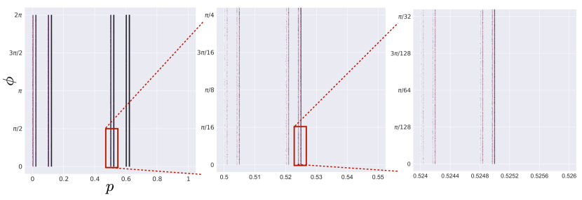
Figure 2: Geometric quantum states visited along a single trajectory generated by the Extended Baker’s Map with parameters $\lambda_{a}=\lambda_{b}=0.2$, $\beta=4\pi/10$, and initial condition $(p_{0},\phi_{0})=(0.32865,0.98886)$. $N=10^{7}$ time-steps plotted on the Bloch square $(p,\phi)\in[0,1]\times[0,2\pi]$. Over time, due to the map’s chaotic nature, even a single trajectory covers a (strange) attractor, with self-similar (fractal) structure. More specifically, vertically, the attractor has a uniform structure. Horizontally, it has self-similar, fractal structure, equivalent to a generalized Cantor set. This is demonstrated, going from the left panel to the right, via successively magnifying small subsets of states.

Examining the operation of partial trace over the position degrees of freedom, for a generic $\ket{\psi}$, we see that it gives rise to a continuous geometric quantum state, parametrized by the coordinates $x$ and $y$:

$$\rho^{S} =\int dxdy|f(x,y)|^{2}\ket{v(x,y)}\bra{v(x,y)}$$

$$=\int d\nu_{FS}^{(p,\phi)}q(p,\phi)\ket{p,\phi}\bra{p,\phi}\leavevmode\nobreak\ ,$$

where $\ket{p,\phi}=\sqrt{1-p}\ket{0}+\sqrt{p}e^{i\phi}\ket{1}$. The second equality in the equation above implicitly defines a distribution on the qubit’s projective Hilbert space. The procedure is detailed in in Ref. [1]. The following simply summarizes the final result.

Given an operator $\mathcal{O}$, acting only on the Hilbert space of the spin, we have the following:

$$\left\langle\mathcal{O}\right\rangle =\int_{x_{0}}^{x_{1}}\!\!\!dx\int_{y_{0}}^{y_{1}}\!\!\!dy|f(x,y)|^{2}\mathcal{O}(v(x,y))$$

$$=\int d\nu_{FS}^{(p,\phi)}\,q(p,\phi)\,O(p,\phi)\leavevmode\nobreak\ ,$$ (12)

where $q$ is a geometric quantum state that depends on $f$ and $d\nu_{FS}^{(p,\phi)}=dpd\phi/2\pi$ indicates the uniform Fubini-Study measure with coordinates $(p,\phi)$. The details of how $q$ depends on $f$ and on the Fubini-Study metric are not immediately relevant, but can be found in Ref. [1]. Here, though, we provide a concrete example to illustrate computing $\mathfrak{D}[q]$ and $H_{\mathfrak{D}}[q]$.

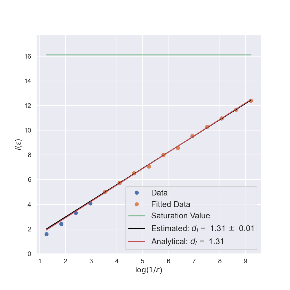
Figure 3: Extended Baker’s Map information dimension $d_{I}$: The estimation incrementally decreases the coarse-graining scale $\epsilon$ and, at each step, calculates $H(Z^{\epsilon})$. Then, excluding some initial points to avoid saturation, it performs a least-square fit to extract the $H(Z^{\epsilon})$’s growth rate as a function of $\log 1/\epsilon$. We estimate $d_{I}=1.31\pm 0.01$. This is fully consistent with the analytical prediction of $d_{I}=1.31$, plotted in red. See Eq. (13) and Ref. [34] for the analytical estimate.

To be concrete, let $p_{1}(x,y)=\frac{x-x_{0}}{x_{1}-x_{0}}$, $\phi_{1}(x,y)=2\pi\frac{y-y_{0}}{y_{1}-y_{0}}$, and $f(x,y)=\sqrt{G(x,y)}$, where $G(x,y)$ is a $2D$ Gaussian on $\mathcal{R}_{2D}$:

$$G(x,y)=\left\{\begin{array}[]{ll}\frac{e^{-\frac{1}{2}\left(\frac{x-\mu_{x}}{\sigma_{x}}\right)^{2}}}{\mathcal{N}_{x}}\frac{e^{-\frac{1}{2}\left(\frac{y-\mu_{y}}{\sigma_{y}}\right)^{2}}}{\mathcal{N}_{y}}\leavevmode\nobreak\ ,&(x,y)\in\mathcal{R}_{2D}\\ &\\ 0&\textrm{otherwise}\end{array}\right.\leavevmode\nobreak\ ,$$

where $(\mu_{x},\sigma_{x})$ and $(\mu_{y},\sigma_{y})$ are the average and variance along the $x$ and $y$ axis, respectively. $\mathcal{N}_{x}$ and $\mathcal{N}_{y}$ are normalization factors.

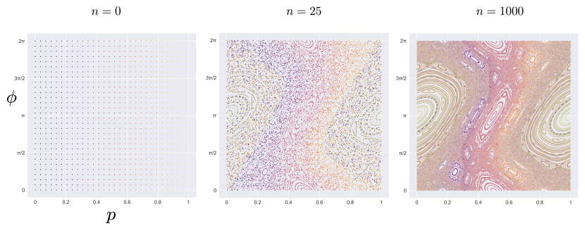
Figure 4: Standard Map on the Bloch Square: Quantum states $(p,\phi)\in[0,1]\times[0,2\pi]$ iterated at $K=1.15$ over a uniform grid of initial conditions. (Left) Initial distribution $n=0$: Homogeneous distribution with $30^{2}$ points $(p_{0}^{(j)},\phi_{0}^{(k)})=(j/30,2\pi k/30)$, with $j,k=0,\ldots,29$ running over all initial conditions, each distinctly colored. (Middle) After only $n=25$ iterations the points begin to mix and exhibit emergent, according to whether they lie in regions of periodic, quasiperiodic, or chaotic behavior. (Right) The long-term distribution, after $n=1000$ iterations. The full range of behavior types is evident.

This constructs a geometric quantum state that is absolutely continuous with respect to $\nu_{FS}$ and therefore expressible via a probability density $q(p,\phi)$. With the choices made, we obtain:

$$q(p,\phi)=2\pi\frac{\mathrm{exp}\left[{-\frac{1}{2}\left(\frac{p-\mu_{p}}{\sigma_{p}}\right)^{2}}\right]}{\mathcal{N}_{p}}\frac{\mathrm{exp}\left[{-\frac{1}{2}\left(\frac{\phi-\mu_{\phi}}{\sigma_{\phi}}\right)^{2}}\right]}{\mathcal{N}_{\phi}}\leavevmode\nobreak\ ,$$

with $\mathcal{N}_{p}\coloneqq\int_{0}^{1}dpe^{-\frac{1}{2}\left(\frac{p-\mu_{p}}{\sigma_{p}}\right)^{2}}$ and $\mathcal{N}_{\phi}\coloneqq\int_{0}^{2\pi}d\phi e^{-\frac{1}{2}\left(\frac{\phi-\mu_{\phi}}{\sigma_{\phi}}\right)^{2}}$. Moreover, $\mu_{p}\coloneqq\frac{\mu_{x}-x_{0}}{x_{0}-x_{1}}$, $\sigma_{p}\coloneqq\frac{\sigma_{x}}{x_{1}-x_{0}}$, $\mu_{\phi}\coloneqq 2\pi\frac{\mu_{y}-y_{0}}{y_{0}-y_{1}}$, and $\sigma_{\phi}\coloneqq\sigma_{y}\frac{2\pi}{y_{1}-y_{0}}$.

What are the quantum information dimension and the dimensional geometric entropy of $q(p,\phi)$? Since this is an absolutely continuous density function, with support on the whole of $\mathcal{P}(\mathcal{H})$, one can directly compute the limit in Eq.(4), obtaining $\mathfrak{D}=2$. Moreover, $H_{2}[Z]$ assumes a particularly simple form due to the Gaussian character of $q(p,\phi)$:

$$H_{2}[Z] =\frac{1}{2}\mathbb{E}\left[\left(\frac{p-\mu_{p}}{\sigma_{p}}\right)^{2}\right]+\frac{1}{2}\mathbb{E}\left[\left(\frac{\phi-\mu_{\phi}}{\sigma_{\phi}}\right)^{2}\right]+$$

$$\qquad+\log\mathcal{N}_{p}+\log\mathcal{N}_{\phi}-\log 2\pi$$

$$=\log\mathcal{N}_{p}+\log\mathcal{N}_{\phi}+\log\frac{e}{2\pi}\leavevmode\nobreak\ .$$

Thus, again, $\mathfrak{D}=2$ correctly addresses the dimensionality of the underlying geometric quantum state and $H_{2}[Z]$ appropriately quantifies its entropy.

V.3 Case 3: Chaotic Dynamics and Quantum Fractals

While the examples above clarify the meaning of, and the technology behind, information dimension, its strength resides in estimating the dimension of complex probability distributions, especially those whose support is fractal [45, 46, 27]. These objects have interesting features, such as structural self-similarity and spontaneous statistical fluctuations, and often arise as invariant distributions of the dynamics of complex systems. The geometric formalism allows us to show how examples imported from the classical theory of dynamical systems, leading up to fractal invariant sets, are part and parcel of the phenomenology of quantum systems. In particular, by exploiting the fact that the Fubini-Study uniform measure on $\mathbb{C}P^{1}$ in $(p,\phi)$ coordinates is proportional to the Lebesgue measure on the square $[0,1]\times[0,2\pi]$, we look at two well-known examples of chaotic dynamical systems with chaotic attractors with fractal support—the Extended Baker’s Map [34] and Chirikov Standard Map [47]. We show how to directly implement them in quantum systems by leveraging geometric quantum mechanics.

V.3.1 Baker’s Map

First, we look at the Extended Baker’s Map (EBM) that, despite the chaotic behaviors it generates, can be analytically solved. For a detailed discussion about its properties, especially those related to the information dimension, we refer to Ref. [34].

This map is directly implemented on $\mathbb{C}P^{1}$ via the following unitary transformations. Let $B$ denote the Extended Baker’s Map, each iteration of $B$ maps a quantum state $(p,\phi)\in\mathbb{C}P^{1}$ to one and only one quantum state $\left(p^{\prime},\phi^{\prime}\right)$.

Definition 1 (Extended Baker’s Map).

$$\left(p^{\prime},\phi^{\prime}\right)=\left\{\begin{array}[]{ll}\left(\lambda_{a}p,2\pi\frac{\phi}{\beta}\right)&\textrm{if $\phi\leq\beta$}\\ &\\ \left(\frac{1}{2}+\lambda_{b}p,2\pi\frac{\phi-\beta}{2\pi-\beta}\right)&\textrm{if $\phi>\beta$}\end{array}\right.\leavevmode\nobreak\ .$$

Here, we use $\lambda_{a}\leq\lambda_{b}\leq\frac{1}{2}$ and $\beta\leq\pi$. Note that the original extended Baker’s Map, as in Ref. [34], is defined on the unit square $(x,y)\in[0,1]\times[0,1]$. The above adapts it to the Bloch square via $(p\to x,\frac{\phi}{2\pi}\to y)$. As a result, $\beta$ is renormalized by a factor $2\pi$ with respect to the one $\alpha$ found in Ref. [34]: $\alpha\to\beta=2\pi\alpha$.

Since there is a one-to-one correspondence between points of the Bloch square and points in $\mathbb{C}P^{1}$, the action $B[(p,\phi)]=(p^{\prime},\phi^{\prime})$ can be implemented on $\mathcal{H}$ as a unitary transformation, as follows.

First, on the qubit Hilbert space, given any $\ket{\psi}$ there is one and only one orthogonal state $\ket{\psi^{\perp}}$, up to normalization and phase. Thus, a unitary transformation that maps $\ket{\psi}$ onto another $\ket{\phi}$ is directly written as $U=\ket{\phi}\bra{\psi}+\ket{\phi^{\perp}}\bra{\psi^{\perp}}$.

Second, embedding of $\mathbb{C}P^{1}$ with $(p,\phi)$ coordinates onto the qubit Hilbert space is given by:

$$(p,\phi)\in\mathbb{C}P^{1}\to\ket{p,\phi}=\sqrt{1-p}\ket{0}+\sqrt{p}e^{i\phi}\ket{1}\in\mathcal{H}\leavevmode\nobreak\ .$$

With this, given a point $(p,\phi)$, the state orthogonal to $\ket{p,\phi}$ is simply $\ket{1-p,\phi+\pi}$. This means $\innerproduct{p,\phi}{1-p,\phi+\pi}=0$ for all $(p,\phi)$. Hence, this results in the unitary $U:=U(B)$ that implements $B$ on the Hilbert space:

$$U=\ket{\psi(p^{\prime},\phi^{\prime})}\bra{\psi(p,\phi)}+\ket{\psi^{\perp}(p^{\prime},\phi^{\prime})}\bra{\psi^{\perp}(p,\phi)}\leavevmode\nobreak\ .$$

As a result, iterates of $U$ directly implement the EBM on $\mathbb{C}P^{1}$. Reference [34] gives a detailed discussion on the map’s dynamic properties. Here, we simply recall that, given an arbitrary initial point $(p_{0},\phi_{0})$, as a result of the dynamics, the point moves on a subset of the entire phase space. Thus, the natural measure, that results from the dynamics over infinite time, is a fractal object. More accurately, the attractor has a uniform distribution over $\phi$ while it has the structure of an extended Cantor set with respect to $p$. See Fig. 2 for a plot of $10^{7}$ map iterates, illustrating the attractor’s self-similar (fractal) structure.

Moreover, its information dimension $d_{I}$ is known analytically:

$$d_{I}(\alpha,\lambda_{a},\lambda_{b})=1+\frac{-\alpha\log\alpha-(1-\alpha)\log(1-\alpha)}{|\alpha\log\lambda_{a}+(1-\alpha)\log\lambda_{b}|},$$ (13)

where $\alpha=\beta/2\pi$. This gives a quantum information dimension $\mathfrak{D}\approx 1.31$ and it allows us to benchmark the numerical procedure we used to compute the information dimension, a necessary reference for cases in which $\mathfrak{D}$ is not known. To extract the dimensional entropy we look at the estimated zero-point of the curve $H(Z^{\epsilon})$ as a function of $-\log\epsilon$. The linear fit gives $H_{\mathfrak{D}}\approx 0.25\pm 0.15$. See Fig. 3.

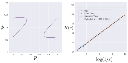
Figure 5: (Left) Periodic orbit with dynamic generated by the Standard Map at $K=2$ and initial conditions $(p_{0},\phi_{0})=(0.2,\pi)$. (Right) Numerical estimation of the information dimension, obtained by extracting the growth rate of $H(\epsilon)$, shorthand for $H(Z^{\epsilon})$, as a function of $\log(1/\epsilon)$. The estimated value is consistent, up to $2$ significant digits, with the expected $\mathfrak{D}=1$.

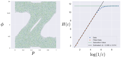
Figure 6: (Left) Chaotic orbit with dynamic generated by the Standard Map at $K=2$ and initial conditions $(p_{0},\phi_{0})=(0.1,4\pi/10)$. (Right) Numerical estimation of the information dimension, as above. Again, the estimated value is consistent, up to $2$ significant digits, with the expected one of $\mathfrak{D}=2$.

Standard Map

Let’s shift attention to the dynamically richer Standard Map (SM). While its original definition is given on the square of side $2\pi$, it is easily modified to operate on the Bloch Square $[0,1]\times[0,2\pi]$, i.e. $\mathbb{C}P^{1}$ in $(p,\phi)$ coordinates.

Definition 2 (Standard Map).

$$\begin{array}[]{l}p^{{}^{\prime}}=p+\frac{K}{2\pi}\sin\phi\\ \\ \phi^{{}^{\prime}}=\phi+2\pi p\leavevmode\nobreak\ ,\end{array}$$

where $p$ is taken modulo $1$, $\phi$ modulo $2\pi$, and $(p_{0},\phi_{0})\in[0,1]\times[0,2\pi]$. $K$ is a nonnegative parameter that determines the map’s degree of nonlinearity. Its value is renormalized by $2\pi$ due to the fact that in its original definition the standard map operates on the unit square $[0,1]\times[0,1]$, while here we work in $(p,\phi)\in[0,1]\times[0,2\pi]$.

The transformation can be implemented with a set of unitary transformations $\{S\}$, using the same construction just described in Sec. V.3 for the EBM.

For $K=0$ only periodic and quasi-periodic orbits are possible. For $K>0$ the map generates regions of chaotic behavior and periodic orbits. Increasing $K$, the extent of periodic orbits decreases, yielding to larger areas of chaotic behavior. Figure 4 shows the behavior at $K=1.15$, where both periodic orbits and chaotic behavior are clearly visible.

As a consequence of the mixed behavior across the state space, the information dimension of the natural measure, computed over a single trajectory, depends on the initial condition. If initial conditions lead to chaotic orbits, then we expect $\mathfrak{D}=2$. While for periodic orbits, we expect $\mathfrak{D}=1$.

We numerically verify this using the same algorithm exploited in the previous section to estimate EBM’s information dimension. Figures 5 and 6 plot the results, consistent with the expected values.

Analogously, for the dimensional entropy there are two different situations, depending on whether the initial condition leads to periodic or chaotic behavior. Since in the chaotic case we simply have a 2D integral, here we look more closely at the second case, in which $\mathfrak{D}=1$, where the following treatment can be applied.

Referring to Fig. 7, a generic periodic orbit covers a $1$-dimensional line, which is identified by a generic equation $f(\phi,p)=0$, whose solutions are parametrized by a curve $\gamma:[0,1]\to\mathbb{C}P^{1}$, or a set of them $\left\{\gamma_{i}\right\}$, as in the case of Fig. 5. In the following, assume that the set of curves $\gamma_{i}$ is bijective, so that given a point $Z$ on any curve, there is one and only one curve the point is part of, thus the functions $\gamma_{i}(s)$ admit inverse $\gamma_{i}^{-1}:\mathbb{C}P^{1}\to[0,1]$. While at first this appears to be a restrictive assumption, one can always use this construction in cases in which there are overlapping curves, simply by decomposing them into nonoverlapping subparts.

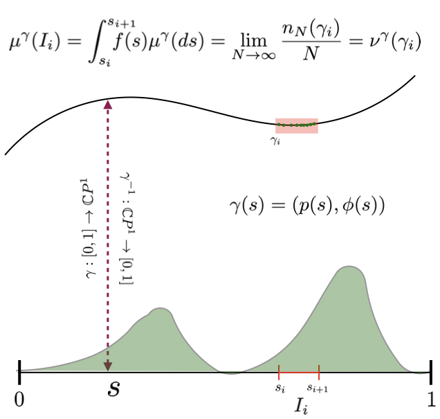
Figure 7: Dimensional quantum entropy of a qubit: Geometric construction for periodic behavior. The construction gives rise to a natural measure of dimension $\mathfrak{D}=1$. The measure’s characteristics on $\mathbb{C}P^{1}$ transfer to a random variable on the unit interval in a way that does not deform the distribution; That is, it keeps intact the probability ratios $\frac{\nu_{\gamma}(\gamma_{i})}{\nu_{\gamma}(\gamma_{j})}=\frac{\mu_{\gamma}(I_{i})}{\mu_{\gamma}(I_{j})}\approx\frac{n(\gamma_{i})}{n(\gamma_{j})}$. This holds thanks to the fact that $\mathfrak{D}=1$ and therefore the support of the measure is a curve, $\gamma$, on $\mathbb{C}P^{1}$, that can always be parametrized by $\gamma(s)$ with $s\in[0,1]$. The green area represents a fictitious probability density on $\gamma$, mapped onto $[0,1]$.

Proceed in this way by analyzing each separately and, since the treatment is formally the same for each, we simply examine one of them and drop the index $i$. The function $\gamma$ is the nonvanishing support of the distribution whose entropy we are evaluating. On $\gamma$, the proper notion of invariant measure is provided by the Fubini-Study infinitesimal length element: $dl_{FS}^{\gamma}$, where $dl_{FS}^{\gamma}\coloneqq||\dot{\gamma}||_{FS}ds$, where $\dot{\gamma}=(\frac{dp}{ds},\frac{d\phi}{ds})$, $||v||_{FS}=\sqrt{g_{ab}^{FS}v^{a}v^{b}}$ is the Fubini-Study norm of a vector $v$ in the tangent space and $g^{FS}$ is the Fubini-Study metric. Thus, the Fubini-Study length of the curve $\gamma$ provides a notion of measure on $[0,1]$ that is invariant under changes of coordinates and by unitary transformations in $\mathbb{C}P^{1}$, via $\mu^{\gamma}_{s}(ds)\coloneqq dl^{\gamma}_{FS}=||\dot{\gamma}(s)||_{FS}ds$. This provides the proper notion of integration on $[0,1]$ to respect all the necessary invariance properties inherited by the fact that the points on $\gamma$ belong to $\mathbb{C}P^{1}$.

Thus, given a measure $\nu^{\gamma}$ on $\mathbb{C}P^{1}$ with support on $\gamma$ and density $d\nu^{\gamma}=\nu(dl^{\gamma}_{FS})=f(s)dl^{\gamma}_{FS}$, the limit in Eq.(7) can be carried out to give:

$$H_{1}[\nu^{\gamma}]\coloneqq-\int_{0}^{1}f(s)\log f(s)d\mu_{s}^{\gamma}(ds)\leavevmode\nobreak\ ,$$

where $f(s)$ is the density or, more appropriately, the Radon-Nikodym derivative, of $\nu^{\gamma}$ with respect to $\mu^{\gamma}$.

For example, one can verify that this procedure gives the expected results in the case of a uniform distribution. Calling $L[\gamma]$ the Fubini-Study length of the curve we have that $f_{unif}(s)=\frac{1}{L[\gamma]}$ and entropy $\log L[\gamma]$. It is worth noting that a most important property of this procedure is that it facilitates computing the entropy of a $1D$ distribution on $\gamma\in\mathbb{C}P^{1}$ by mapping it into the entropy of a continuous density on $[0,1]$. This amounts to defining $f$ as the continuous density that satisfies the following consistency constraint: For any arbitrary finite partitioning $[0,1]=\cup_{i}I_{i}$, that generate a partition of $\gamma$ into a set of $N$ adjacent curves, $\gamma=\cup_{i}\gamma_{i}$, where $\gamma_{i}=\gamma(I_{i})$, the density $f$ is defined via the following chain of equalities:

$$\nu^{\gamma}(\gamma_{i}) =\lim_{N\to\infty}\frac{n_{N}(\gamma_{i})}{N}$$

$$=\int_{I_{i}}f(s)\mu^{\gamma}(ds)$$

$$=\mu^{\gamma}(I_{i})\leavevmode\nobreak\ ,$$

for any $i$ and where $n_{N}(\gamma_{i})$ is the number of points belonging to $\gamma_{i}$ in a finite (size $N$) sample of the density on $\gamma$. This construction provides a constructive method to compute analytically $H_{1}$, provided one has the form of $\gamma$ and $f(s)$. It also gives a direct way to numerically estimate $H_{1}$, via the sampling provided by the dynamics: $n_{N}(\gamma_{i})/N\approx\nu_{\gamma}(I_{i})$ when $N\gg 1$.

V.4 Case 4: Thermodynamic Limit

Finally, let’s shift to explore dimensions for an overtly physical setting: a finite quantum system without symmetry that interacts with a finite, but arbitrarily large, environment. The goal is to infer properties in the thermodynamic limit. The generic procedure to investigate the thermodynamic limit in geometric quantum mechanics was established and made explicit in Ref. [1]. The following adopts that procedure and investigates the geometric quantum state of the ground state of an open-boundary $1D$ spin-$1/2$ Heisenberg chain with a broken translational symmetry, a defect, made by removing the local magnetic field in the last qubit.

Let $\vec{\tau}$ be the system’s spin operator and $\vec{\sigma}_{j}$ the environment’s spin operators. The total Hamiltonian is:

$$H=H_{S}+H_{E}(N_{E})+H_{\mathrm{int}}(N_{E})\leavevmode\nobreak\ ,$$

where $N_{E}$ is the size of the environment, $H_{S}=\vec{B}\cdot\vec{\tau}$, and:

$$H_{E}(N)=\sum_{k=1}^{N_{E}-1}\vec{\sigma}_{k}\cdot\vec{\sigma_{k+1}}+\vec{B}\cdot\vec{\sigma}_{k}\leavevmode\nobreak\ ,$$

$$H_{\mathrm{int}}=\vec{\tau}\cdot\vec{\sigma}_{1}\leavevmode\nobreak\ .$$ (14)

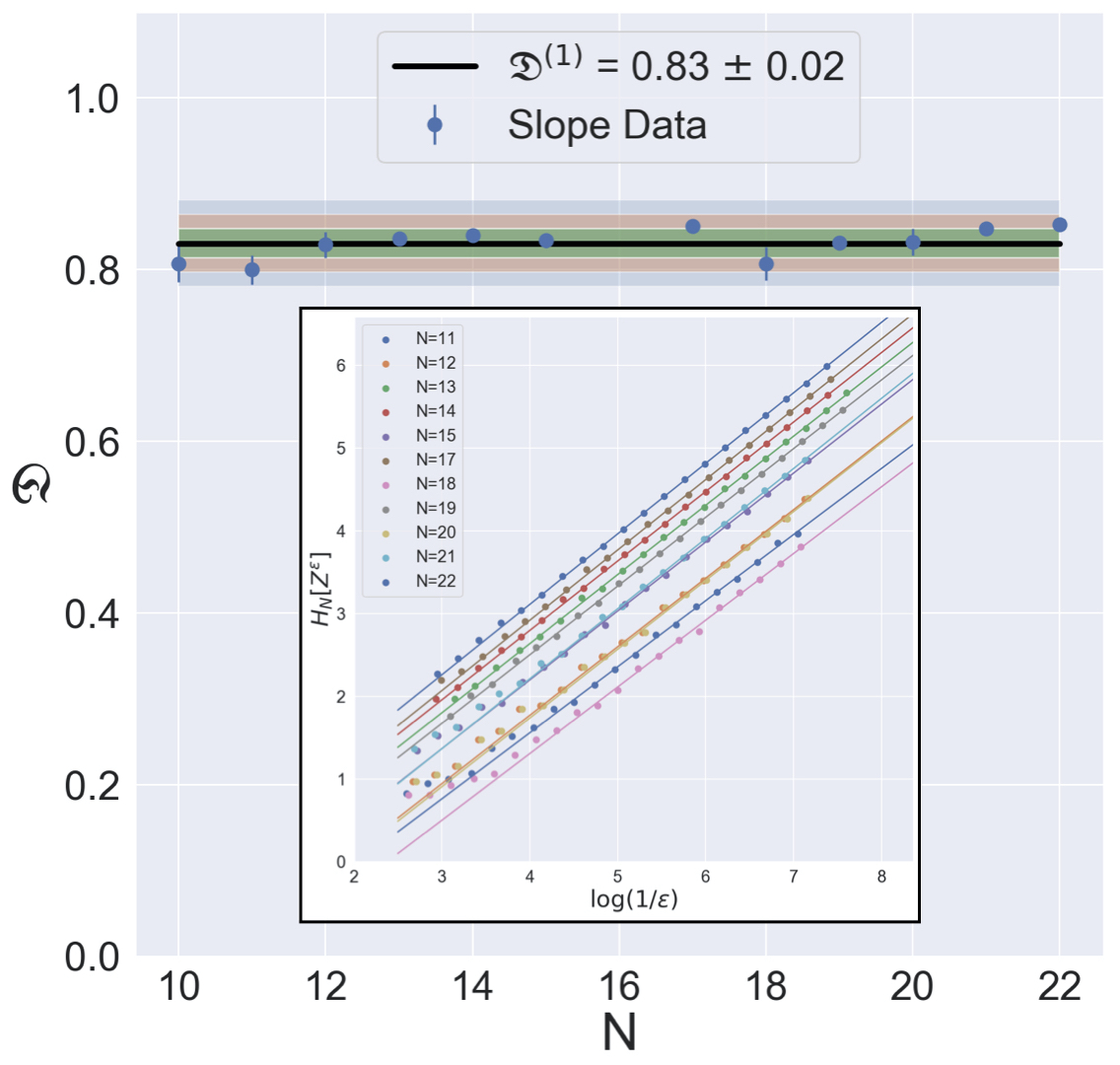
Figure 8: Information dimension of the geometric quantum state of a qubit interacting with a $1D$ environment with a defective (i.e., nontranslation invariant) Heisenberg model of progressively increasing size, see Eq. (14). The entire system is in its ground state $\ket{GS(N)}$, where the environment size is $N\in[10,22]$. Each $N$ yields a geometric quantum state whose information dimension we estimate using the box-counting algorithm explained in the text, extracting the slope using a linear fit for $H_{N}[Z^{\epsilon}]$. (Inset) A collection of all the data, together with the linear fits. (Overall) The collection of horizontal lines displays all $M=13$ estimates and extracts the average and standard deviation. The result yields $\mathfrak{D}^{(1)}=0.83\pm 0.02$. The shaded area in green, red, and blue correspond to the areas covered by fluctuations around the average of size $\sigma,2\sigma$, and $3\sigma$, respectively, where $\sigma=0.02$ is the standard deviation of the sample of slopes.

The defect-bearing Hamiltonian breaks translational symmetry creating a rich geometric quantum state—one that exhibits self-similarity and fractal structure. As we will see, the choice is supported by the numerical analysis. For the latter we used $B_{z}=0.5$ and $N\in[10,22]$. At each size $N$ we used the Lanczos algorithm, available in Python via SciPy, to extract the ground state $\ket{\mathrm{GS}(N)}$ and calculate the system’s associated geometric quantum state $q_{N}(Z)$. Then, for each environment size, we estimate the information dimension using the numerical procedure used and benchmarked in previous sections. This provides $M=13$ different datasets to estimate the value of $\mathfrak{D}$.

The estimation was completed in two separate ways, each yielding compatible results. First, a linear fit was performed by identifying a common region of linearity for all the $13$ curves $H_{N}[Z^{\epsilon}]\propto\mathfrak{D}^{(1)}(-\log\epsilon)$ analyzed. Then, from the $13$ averages we estimated the information dimension (and its error) from the average and standard deviation. The results yield $\mathfrak{D}^{(1)}=0.83\pm 0.02$ and are summarized in Fig. 8. Second, we collapsed all the data onto a unique straight line by removing their estimated vertical offset (setting intercept equal to $0$). We removed a single outlier, to reduce the error, and checked that this does not appreciably change the estimation. We then performed linear regression on the aggregated data points. The results yield $\mathfrak{D}^{(2)}=0.84\pm 0.01$ and are summarized in Fig. 9.

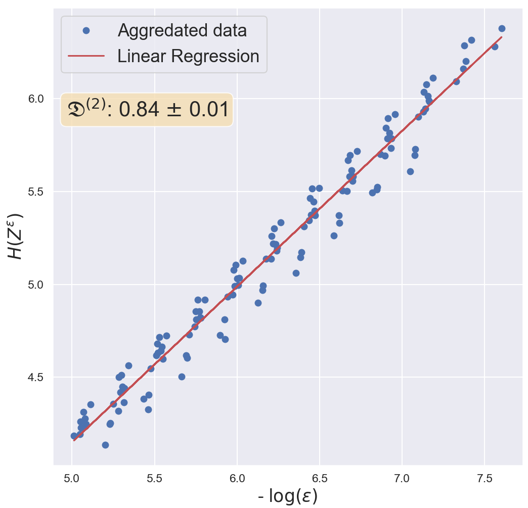
Figure 9: Information dimension of the same geometric quantum state, estimated using aggregated data. To extract the information dimension in the thermodynamic limit, we do not distinguish between points belonging to different environment sizes. Aggregating them, we performed linear regression to extract a prediction, with associated error, of the curve’s slope. The result yields $\mathfrak{D}^{(2)}=0.84\pm 0.01$.

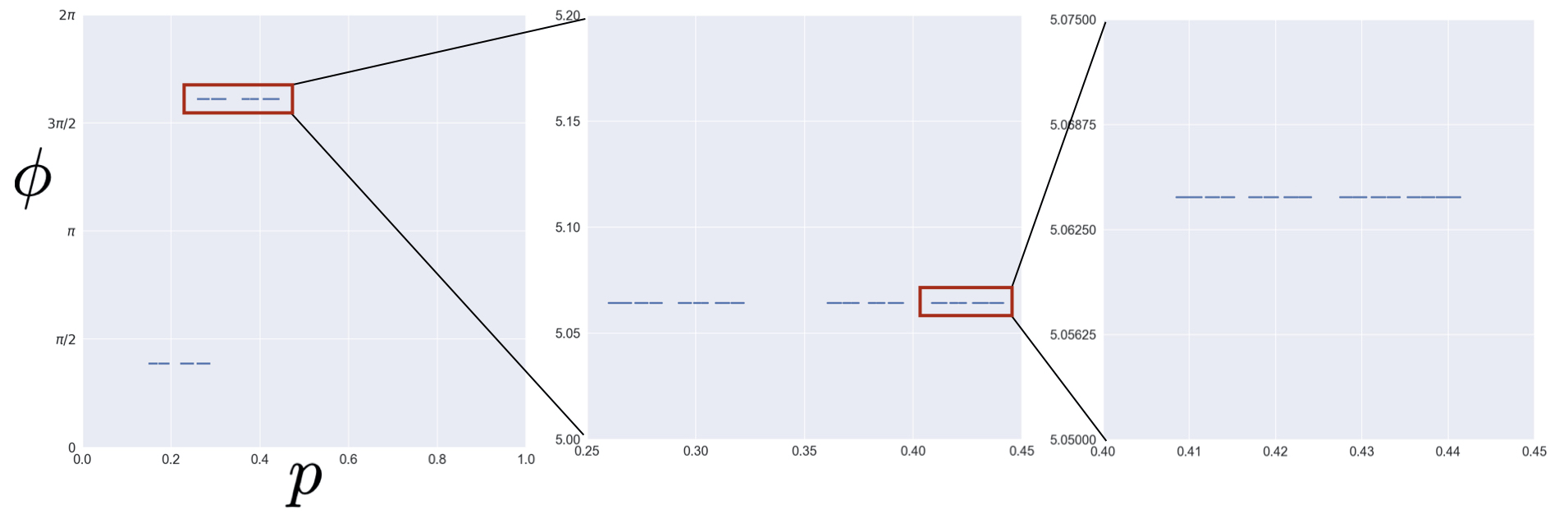
Figure 10: Support of the geometric quantum state $\ket{GS(N_{E})}$ for the ground state of the Heisenberg defect-Hamiltonian with environment size $N=22$. The GQS has two separate islands with internal structure that is self-similar. (Left to Middle to Right panels) Progressively magnifying the region around each part of the support reveals the distribution’s self-similar support, whose information dimension has been previously estimated, in the thermodynamic limit, to be $\mathfrak{D}\approx 0.83\pm 0.02$.

Altogether, the results support the intuition that the thermodynamic limit is witness to highly nontrivial geometric quantum states with fractal support. Increasing the environment’s size, the system converges to a self-similar distribution, with a noninteger information dimension $\mathfrak{D}\approx 0.83\pm 0.02$. The state set shown in Fig. 10 is reminiscent of the Cantor set or, more appropriately, one of its generalizations, e.g., the EBM’s invariant distribution in the $x$ direction.

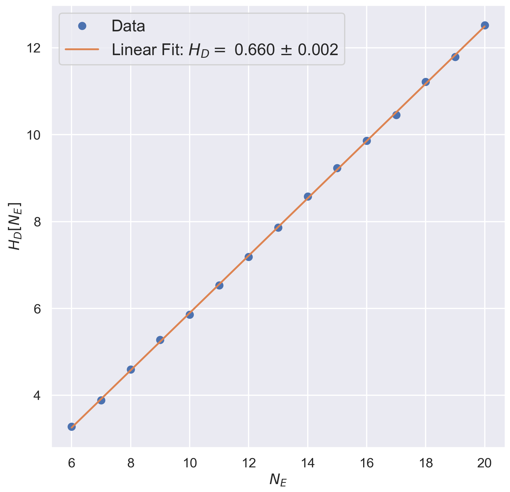
Figure 11: Dimensional quantum entropy $H[N_{E}]$ scaling in the geometric quantum state $q$ as a function of environment size $N_{E}$. The estimated linear growth $H[N_{E}]\sim 0.66N_{E}$ and so the state has entropy rate of $0.66$.

Here, when estimating the dimensional geometric entropy, the situation differs from the previous examples, as we are not exploring dynamical properties. Rather, we probe how the system’s geometric quantum state changes as a function of the environment’s dimension, assuming that the entire system is always in the ground state $\ket{GS(N_{E})}$ of a joint Hamiltonian $H_{SE}(N_{E})$. Since at each fixed $N_{E}$ the environment has finite size, we can directly compute the geometric entropy via its definition, given explicitly in Thm. 3 and extract its linear asymptote, giving the geometric entropy rate $h$ in the thermodynamic limit as:

$$h:=\lim_{N_{E}\to\infty}\frac{H(N_{E})}{N_{E}}\leavevmode\nobreak\ .$$

Thanks to the convergence to linear scaling occurring rather quickly, an accurate estimate of $h$ is obtained directly from the data. Thus, we have a reliable estimate up to two significant digits: $h\approx h_{est}=0.66\approx 95\%\log 2$. Both data and the results of the linear fit are given in Fig. 11.

This concludes the survey of range of informational properties of geometric quantum states. Table 1 summarizes the results. The results leave several questions and points of discussion, to which we now turn. After which we draw several conclusions.

	$\mathfrak{D}$	$H_{\mathfrak{D}}$
Case 1 (Finite Env)	0	$-\sum_{\alpha}p_{\alpha}\log p_{\alpha}$
Case 2 ($e^{-}$ Box)	2	$\log\mathcal{N}_{p}+\log\mathcal{N}_{\phi}+\log\frac{e}{2\pi}$
Case 3 (Baker’s Map)	$1.31\pm 0.01$	$0.25\pm 0.15$
Case 3 (SM-Periodic)	1	$-\int_{0}^{1}f(s)\log f(s)\mu^{\gamma}(ds)$
Case 3 (SM-Chaotic)	2	$-\int_{\!\mathbb{C}P^{1}}\!d\nu_{FS}q(Z)\log q(Z)$
Case 4 (Thermo)	0.83	$0.66N_{E}$

Table 1: Quantum information dimensions and dimensional quantum entropies for the geometric quantum states analyzed in Secs. V.1-V.4.

VI Discussion

It has been over a half century since Kolmogorov and followers showed that Shannon’s information theory [2] provides essential dynamical invariants for chaotic physical systems [3, 4, 5, 6, 7, 8]. Today, practically, we know that information theory readily applies to physical systems that evolve in discrete time with either a discrete state space or tractable symbolic dynamics [48]. Applying the Shannon entropy functional, this involves quantities that capture informational features with physical relevance—such as, a system’s randomness and structure. This approach has successfully described the behavior of both Hamiltonian and dissipative classical systems. That said, the situation is decidedly less straightforward for physical systems with an inherently continuous sample space that lack a straightforward symbolic dynamics. Relying on analog information theory, informational descriptions are markedly more challenging to define and calculate.

Quantum systems belong to this category, as the space $\mathcal{P}(\mathcal{H})$ of pure states has continuous nature. Geometric quantum mechanics brings this particular aspect of quantum systems to the fore, describing their states as probability measures on $\mathcal{P}(\mathcal{H})$—that is, in terms of geometric quantum states. Thus, the geometric approach directly leads one to adapt the tools from analog information theory to the quantum domain.

In this spirit, our development focused on information dimension and differential entropy, initially proposed by Renyi within the context of analog information theory. We showed that these tools provide a synthetic view of a system’s geometric quantum state: the information dimension $\mathfrak{D}$ determines the dimensionality of the state’s support, while the dimensional geometric entropy $H_{\mathfrak{D}}$ gives an appropriate differential entropy for a geometric quantum state with information dimension $\mathfrak{D}$. Once defined and properly interpreted, we explicitly computed their values in several examples: a finite-dimensional quantum system interacting with finite and infinite environments; a qubit evolving with quantum implementations of nonlinear maps—the Extended Baker’s Map and the Standard Map—and finally a qubit in a progressively larger environment, where we extracted properties in the thermodynamic limit.

The interest for these investigations is twofold. On the one hand, extending the tools of dynamical systems theory to the quantum domain is a topic of broad and long-lived interest. In point of fact, dynamical systems has led to successful modeling and quantitative understanding of the structures and behaviors generated by large classes of synthetic and natural systems—from nonlinear dynamics to the modeling of population dynamics to tackling the underlying dynamics of information occurring in a computer running classical algorithms. On the other hand, the phenomenology of open quantum systems, in equilibrium and far from equilibrium, is a topic of both fundamental and applied relevance. Indeed, in the past half decade, the rise of the quantum computing paradigm made concrete several theoretical investigations focused on the information-theoretic properties embedded in the dynamics of open quantum systems and the thermodynamic resources necessary for quantum information processors to run smoothly and efficiently.

We believe the geometric approach is well suited for these goals, for the following reasons. The notion of geometric quantum state of a system [1] encodes not only the statistics of all measurement outcomes one can perform on the system, as with the density matrix, but also the detailed structure of the system-environment quantum correlations that determine said measurement statistics. Hence, determining the information-theoretic properties of geometric quantum states gives a novel way to understand the phenomenology of open quantum systems, whose behavior and structure result from exchanging information-theoretic and energetic resources with an environment. We believe this will eventually lead to new analytical tools of power sufficient to deepen our understanding of the phenomenology of open quantum systems, both in and out of equilibrium.

VII Conclusions

The development’s overtly mathematical nature suggests concluding with two forward-looking comments. First, simple examples of geometric quantum states yield an integer value for $\mathfrak{D}$. At least in the measure theory of classical processes, though, it is well-known that this is not typical. There are very interesting objects that exhibit noninteger information dimension: the self-similar or Cantor sets, now shorthanded as fractals. Indeed, these structures are critical to the operation of Maxwellian demons [49] and their modern cousins—information engines [50]. Comparing classical and quantum domains, it stands to reason that the geometric quantum formalism provides an interesting arena in which to develop a theory of quantum fractals. Efforts in this direction are currently ongoing and will be reported elsewhere. The informational quantities introduced here play a central role in this endeavor.

Second, while focused here exclusively on $\mathfrak{D}$ and $H_{\mathfrak{D}}$, it is straightforward to appreciate that the geometric approach allows for a richer cross-pollination between analog information theory and quantum information theory. For example, alternative definitions for core quantities of quantum information theory, based on the geometric approach and inspired by analog information theory, suggest themselves as parallels of entropy, relative entropy, mutual information, Kolmogorov-Sinai entropy rate, excess entropy, bound information, statistical complexity, and many others. Investigating the relations with their standard quantum counterparts—von Neumann entropy, quantum mutual information, and the like—presents interesting challenges. The solutions, we believe, are destined to enrich both quantum information science and analog information theory.

Appendix A Weak law of large numbers for geometric quantum states

The following provides a direct proof of the weak law of large numbers for real functions on $\mathcal{P}(\mathcal{H})$. First, let’s set up the problem, focusing on quantum systems with Hilbert space $\mathcal{H}$ of arbitrary dimension $D$. The projective space of pure states is $\mathcal{P}(\mathcal{H})$, with dimension $D-1$. A random quantum variable $Z$ is a triple $(\mathcal{P}(\mathcal{H}),\mathcal{B},\mu_{Z})$ where $\mathcal{P}(\mathcal{H})$ is the projective Hilbert space of pure states, $\mathcal{B}$ is its Borel $\sigma-$algebra and $\mu_{Z}$ is a measure on $\mathcal{P}(\mathcal{H})$ such that:

$$\mu(Z)=\int_{S}\mu_{Z}(d\nu_{FS})\leavevmode\nobreak\ ,$$

where $d\nu_{FS}$ is the normalized Fubini-Study measure:

$$\nu_{FS}(S) =\int_{S}d\nu_{FS}$$

$$=\frac{1}{\mathrm{Vol}(\mathcal{P}(\mathcal{H}))}\int_{S}dV_{FS}$$

$$=\frac{\mathrm{Vol}(S)}{\mathrm{Vol}(\mathcal{P}(\mathcal{H}))}\leavevmode\nobreak\ .$$

Now, if $\mu_{Z}$ is absolutely continuous with respect to $d\nu_{FS}$, we have a probability density function $d\mu_{Z}=q(z)d\nu_{FS}$.

Let $\{Z_{k}\}_{k=1}^{N}$ be a series of $N$ random quantum variables. We are interested in the case in which the $Z_{k}$ are all independent and identically distributed. Take a measurable function $f:\mathcal{P}(\mathcal{H})\to\mathbb{R}$. Call $X_{k}\coloneqq f(Z_{k})$. This is a random variable with values on $\mathbb{R}$ with a law we call $\nu_{k}$. The $X_{k}$ with measures $\nu_{k}$ are also i.i.d.. Thus, taking $\overline{x}\coloneqq\mathbb{E}[X_{k}]$ and $\sigma=\mathbb{E}[(X_{k}-\overline{x})^{2}]$, we can define:

$$Y_{k} \coloneqq\frac{X_{k}-\overline{x}}{\sigma}\leavevmode\nobreak\ \text{and}$$

$$Y_{N} \coloneqq\sum_{k=1}^{N}\frac{Y_{k}}{\sqrt{N}}\leavevmode\nobreak\ .$$

Now, let $\phi_{X}(t)\coloneqq\mathbb{E}[e^{itX}]$, we have:

$$\phi_{Y_{N}}(t) =\prod_{k=1}^{N}\phi_{Y_{k}}(\frac{t}{\sqrt{N}})$$

$$=\left[\phi_{Y_{k}}(\frac{t}{\sqrt{N}})\right]^{N}\leavevmode\nobreak\ .$$

Since we are interested in the limit $N\to\infty$, we expand to see that:

$$\phi_{Y_{N}}(t) =\left[\phi_{Y_{k}}(\frac{t}{\sqrt{N}})\right]^{N}$$

$$=\left[1-\frac{t}{2N}+o\left(\frac{t^{2}}{N}\right)\right]^{N}$$

means that:

$$\phi_{Y_{N}}(t)\to\phi_{Y}(t)\propto e^{-\frac{t^{2}}{2}}\leavevmode\nobreak\ .$$

This is a uniform convergence between characteristic functions that, by means of Levy continuity theorem, becomes weak convergence between random variables: $Y_{N}\to Y$. Here $Y\sim\mathcal{N}(0,1)$ since the standardized normal distribution is the only one with characteristic function $\propto e^{-\frac{t^{2}}{2}}$. In turn, this means:

$$\overline{X}_{N} \coloneqq\frac{1}{N}\sum_{k=1}^{N}X_{k}$$

$$=\frac{1}{N}\sum_{k=1}^{N}f(Z_{k})$$

implies:

$$\overline{X}_{N}\sim\mathcal{N}(\overline{x},\sigma_{N})\leavevmode\nobreak\ ,$$

where $\sigma_{N}\coloneqq\frac{\sigma}{\sqrt{N}}$.

Since $\sigma_{N}\to 0$, we denote this convergence $\overline{X}_{N}\to\overline{x}$, where $\overline{x}=\mathbb{E}[X_{k}]=\mathbb{E}[f(Z_{k})]$ and fluctuations are of the order $\sigma/\sqrt{N}$. In other words:

$$\frac{1}{N}\sum_{k=1}^{N}f(Z_{k})$$

converges to:

$$\mathbb{E}[f(Z_{1})]=\int_{\mathcal{P}(\mathcal{H})}f(z)q(z)d\nu_{FS}\leavevmode\nobreak\ .$$

Thus, for example, one can use $f(Z)=-\log q(Z)$, which is measurable as long as the geometric entropy is finite. In this way, one finds that:

$$\lim_{N\to\infty}\frac{1}{N}\sum_{k=1}^{N}-\log q(Z_{k}) =\mathbb{E}[-\log q(Z)]$$

$$=-\int_{\mathcal{P}(\mathcal{H})}q(Z)\log q(Z)$$

$$=H_{\mathfrak{D}}[Z]\leavevmode\nobreak\ .$$

This establishes the weak law of large numbers for a real measurable function $f$ on $\mathcal{P}(\mathcal{H})$ and, in turn, provides a direct proof for the quantum AEP.

Appendix B Electron in a 2D box

The following lays out the detailed calculations for the geometric quantum state in Sec. V.2: an electron in a $2D$ rectangular box. The Hilbert space is given by $\mathcal{P}(\mathcal{H}_{x}\otimes\mathcal{H}_{s})$, where $\mathcal{H}_{x}$ is the infinite dimensional Hilbert space of a quantum particle in a $2D$ box, with basis $\left\{\ket{x,y}\right\}_{x,y}$ and $x\in[x_{0},x_{1}]$, $y\in[y_{0},y_{1}]$. $\mathcal{H}_{s}$, is a qubit Hilbert space describing the spin-1/2 degree of freedom, with reference basis $\left\{\ket{0},\ket{1}\right\}$.

Thus, the discrete degrees of freedom of the system—simply spin-$1/2$ in this case—are described by $f(x,y)$ and $\left\{p_{s}(x,y),\phi_{s}(x,y)\right\}_{s=0,1}$. Then, Eq. (12) becomes:

$$\left\langle\mathcal{O}\right\rangle =\int_{x_{0}}^{x_{1}}\!\!\!dx\int_{y_{0}}^{y_{1}}\!\!\!dy|f(x,y)|^{2}\mathcal{O}(v(x,y))$$

$$=\frac{1}{2}\int_{0}^{1}\!\!\!dp\int_{0}^{2\pi}\!\!\!\!\!d\phi\,q(p,\phi)\,O(p,\phi)\leavevmode\nobreak\ ,$$

where, $p_{0}(x,y)=1-p_{1}(x,y)$, $p_{1}(x,y)=p(x,y)$, $\phi_{0}(x,y)=0$, and $\phi_{1}(x,y)=\phi(x,y)$.

To be concrete take $p(x,y)=\frac{x-x_{0}}{x_{1}-x_{0}}$, $\phi(x,y)=2\pi\frac{y-y_{0}}{y_{1}-y_{0}}$, and $f(x,y)=\sqrt{G(x,y)}$, where $G(x,y)$ is a $2D$ Gaussian on $\mathcal{R}_{2D}$:

$$G(x,y)=\left\{\begin{array}[]{ll}\frac{e^{-\frac{1}{2}\left(\frac{x-\mu_{x}}{\sigma_{x}}\right)^{2}}}{\mathcal{N}_{x}}\frac{e^{-\frac{1}{2}\left(\frac{y-\mu_{y}}{\sigma_{y}}\right)^{2}}}{\mathcal{N}_{y}}\leavevmode\nobreak\ ,&(x,y)\in\mathcal{R}_{2D}\\ &\\ 0&\textrm{otherwise}\end{array}\right.\leavevmode\nobreak\ ,$$

where $(\mu_{x},\sigma_{x})$ and $(\mu_{y},\sigma_{y})$ are the average and variance along the $x$ and $y$ axis, respectively. $\mathcal{N}_{x}$ and $\mathcal{N}_{y}$ are normalization factors.

Using the definitions of the embedding functions, we obtain the following set of spin vectors, parametrized by $\vec{x}=(x,y)$:

$$\ket{v(x,y)}=\sqrt{\frac{x_{1}-x}{x_{1}-x_{0}}}\ket{0}+\sqrt{\frac{x-x_{0}}{x_{1}-x_{0}}}e^{i2\pi\frac{y-y_{0}}{y_{1}-y_{0}}}\ket{1}\leavevmode\nobreak\ .$$

In turn, this gives:

$$\mathcal{O}(v(x,y)) =\bra{v(x,y)}\mathcal{O}\ket{v(x,y)}$$

$$=\frac{x_{1}-x}{x_{1}-x_{0}}\mathcal{O}_{00}+\frac{x-x_{0}}{x_{1}-x_{0}}\mathcal{O}_{11}+\sqrt{\frac{x_{1}-x}{x_{1}-x_{0}}\frac{x-x_{0}}{x_{1}-x_{0}}}\left(\mathcal{O}_{01}e^{i2\pi\frac{y-y_{0}}{y_{1}-y_{0}}}+\frac{x-x_{0}}{x_{1}-x_{0}}e^{-i2\pi\frac{y-y_{0}}{y_{1}-y_{0}}}\mathcal{O}_{10}\right)\leavevmode\nobreak\ .$$

The determinant of the Jacobian matrix between the coordinates $(x,y)$ on $\mathcal{R}_{2D}$ and $(p,\phi)\in[0,1]\times[0,2\pi]$ parametrizing $\mathcal{P}(\mathcal{H}_{1}^{2})\sim\mathbb{C}P^{1}$ is extracted inverting the functions $p(x,y)$ and $\phi(x,y)$:

$$x(p,\phi) =x_{0}+p(x_{1}-x_{0})\leavevmode\nobreak\ \text{and}$$

$$y(p,\phi) =y_{0}+\frac{\phi}{2\pi}(y_{1}-y_{0})\leavevmode\nobreak\ .$$

This gives $D\Phi(Z)=(x_{1}-x_{0})(y_{1}-y_{0})/2\pi$, which in this case is a constant. Then, we have, as expected:

$$\mathcal{O}(v(x,y)) =\mathcal{O}(v(x(p,\phi),y(p,\phi)))$$

$$=(1-p)\mathcal{O}_{00}+p\mathcal{O}_{11}+\sqrt{p(1-p)}\left(\mathcal{O}_{01}e^{i\phi}+\mathcal{O}_{10}e^{-i\phi}\right)$$

and

$$G(x(p,\phi),y(p,\phi))=\left\{\begin{array}[]{ll}\frac{1}{\mathcal{N}_{x}}\mathrm{exp}\left[{-\frac{1}{2}\left(\frac{x_{0}+p(x_{1}-x_{0})-\mu_{x}}{\sigma_{x}}\right)^{2}}\right]\frac{1}{\mathcal{N}_{y}}\mathrm{exp}\left[{-\frac{1}{2}\left(\frac{y_{0}+\frac{\phi}{2\pi}(y_{1}-y_{0})-\mu_{y}}{\sigma_{y}}\right)^{2}}\right]\leavevmode\nobreak\ ,&(p,\phi)\in[0,1]\times[0,2\pi]\\ &\\ 0&\textrm{otherwise}\end{array}\right.\leavevmode\nobreak\ .$$

Eventually, using $dV_{FS}^{\mathbb{C}P^{1}}=\frac{1}{2}dpd\phi$, we can see that $\sqrt{\det g_{FS}(p,\phi)}=1/2$. Calling $G(x(p,\phi),y(p,\phi))=\tilde{G}(p,\phi)$, the geometric quantum state is:

$$q(p,\phi) =\frac{(x_{1}-x_{0})(y_{1}-y_{0})}{2\pi}\times 2\times\tilde{G}(p,\phi)$$

$$=\frac{(x_{1}-x_{0})(y_{1}-y_{0})}{\pi}\tilde{G}(p,\phi)\leavevmode\nobreak\ .$$

This can be written as:

$$q(p,\phi)=2\frac{1}{\mathcal{N}_{p}}\mathrm{exp}\left[{-\frac{1}{2}\left(\frac{\mu_{p}-p}{\sigma_{p}}\right)^{2}}\right]\frac{1}{\mathcal{N}_{\phi}}\mathrm{exp}\left[{-\frac{1}{2}\left(\frac{\phi-\mu_{\phi}}{\sigma_{\phi}}\right)^{2}}\right]\leavevmode\nobreak\ ,$$

with $(p,\phi)\in[0,1]\times[0,2\pi]$, $\mathcal{N}_{p}\coloneqq\int_{0}^{1}dpe^{-\frac{1}{2}\left(\frac{p-\mu_{p}}{\sigma_{p}}\right)^{2}}$, and $\mathcal{N}_{\phi}\coloneqq\int_{0}^{2\pi}d\phi e^{-\frac{1}{2}\left(\frac{\phi-\mu_{\phi}}{\sigma_{\phi}}\right)^{2}}$. Moreover, $\mu_{p}\coloneqq\frac{\mu_{x}-x_{0}}{x_{0}-x_{1}}$, $\sigma_{p}\coloneqq\frac{\sigma_{x}}{x_{1}-x_{0}}$, $\mu_{\phi}\coloneqq 2\pi\frac{\mu_{y}-y_{0}}{y_{0}-y_{1}}$ and $\sigma_{\phi}\coloneqq\sigma_{y}\frac{2\pi}{y_{1}-y_{0}}$.

$q(p,\phi)$ is positive and one straightforwardly verifies that it is normalized. Recall in $(p,\phi)$ coordinates that $dV_{FS}^{(p,\phi)}=dpd\phi/2$ and so:

$$\int_{\mathcal{P}(\mathcal{H}_{1}^{2})}\!\!\!\!\!\!\!\!\!\!dV_{FS}\,\,q(p,\phi) =2\frac{1}{2}\int_{0}^{1}dp\frac{1}{\mathcal{N}_{p}}e^{-\frac{1}{2}\left(\frac{p-\mu_{p}}{\sigma_{p}}\right)^{2}}\int_{0}^{2\pi}d\phi\frac{e^{-\frac{1}{2}\left(\frac{\phi-\mu_{\phi}}{\sigma_{\phi}}\right)^{2}}}{\mathcal{N}_{\phi}}$$

$$=\frac{\mathcal{N}_{p}}{\mathcal{N}_{p}}\frac{\mathcal{N}_{\phi}}{\mathcal{N}_{\phi}}$$

$$=1\leavevmode\nobreak\ .$$

References

- [1] F. Anza and J. P. Crutchfield. Beyond density matrices: Geometric quantum states. Phys. Rev. A, 103:062218, 2021.
- [2] C. E. Shannon. A mathematical theory of communication. Bell Sys. Tech. J., 27:379–423, 623–656, 1948.
- [3] I. M. Gelfand, A. N. Kolmogorov, and I. M. Yaglom. Towards a general definition of the quantity of information. Dokl. Akad. Nauk SSSR, 111:745–748, 1956.
- [4] A. N. Kolmogorov. On the Shannon theory of information transmission in the case of continuous signals. IRE Trans. Info. Th., 2(4):102–108, 1956.
- [5] A. N. Kolmogorov and V. M. Tikhomirov. -entropy and -capacity of sets in function spaces. Uspekhi Mat. Nauk., 14:3, 1959. (Math. Rev. 22, No. 2890).
- [6] A. N. Kolmogorov. A new metric invariant of transient dynamical systems and automorphisms in Lebesgue spaces. Dokl. Akad. Nauk. SSSR, 119:861, 1958. (Russian) Math. Rev. vol. 21, no. 2035a.
- [7] A. N. Kolmogorov. Entropy per unit time as a metric invariant of automorphisms. Dokl. Akad. Nauk. SSSR, 124:754, 1959. (Russian) Math. Rev. vol. 21, no. 2035b.
- [8] Ja. G. Sinai. On the notion of entropy of a dynamical system. Dokl. Akad. Nauk. SSSR, 124:768, 1959.
- [9] F. Strocchi. Complex coordinates and quantum mechanics. Rev. Mod. Phys., 38(1):36–40, 1966.
- [10] B. Mielnik. Geometry of quantum states. Comm. Math. Phys., 9:55–80, 1968.
- [11] T. W. B. Kibble. Geometrization of quantum mechanics. Comm. Math. Physics, 65(2):189–201, 1979.
- [12] A. Heslot. Quantum mechanics as a classical theory. Phys. Rev. D, 31(6):1341–1348, 1985.
- [13] D. Page. Geometrical description of Berry’s phase. Phys. Rev. A, 36, 1987.
- [14] J. Anandan and Y. Ahronov. Geometry of quantum evolution. Phys. Rev. Lett., 65, 1990.
- [15] G. W. Gibbons. Typical states and density matrices. J. Geom. Physics, 8(1-4):147–162, 1992.
- [16] A. Ashtekar and T. A. Schilling. Geometry of quantum mechanics. In AIP Conference Proceedings, volume 342, pages 471–478. AIP, 1995.
- [17] A. Ashtekar and T. A. Schilling. Geometrical formulation of quantum mechanics. In On Einstein’s Path, pages 23–65. Springer New York, New York, NY, 1999.
- [18] D. C. Brody and L. P. Hughston. Geometric quantum mechanics. J. Geom. Physics, 38(1):19–53, 2001.
- [19] J. F. Cariñena, J. Clemente-Gallardo, and G. Marmo. Geometrization of quantum mechanics. Theo. Math. Physics, 152(1):894–903, jul 2007.
- [20] D. Chruściński. Geometric aspects of quantum mechanics and quantum entanglement. J. Physics: Conf. Ser., 30:9–16, 2006.
- [21] G. Marmo and G. F. Volkert. Geometrical description of quantum mechanics—transformations and dynamics. Physica Scripta, 82(3):038117, 2010.
- [22] J. Avron and O. Kenneth. An elementary introduction to the geometry of quantum states with pictures. Rev. Math. Physics, 32(02):2030001, 2020.
- [23] D. Pastorello. A geometric Hamiltonian description of composite quantum systems and quantum entanglement. Intl. J. Geo. Meth. Mod. Physics, 12(07):1550069, 2015.
- [24] D. Pastorello. Geometric Hamiltonian formulation of quantum mechanics in complex projective spaces. Intl. J. Geom. Meth. Mod. Physics, 12(08):1560015, 2015.
- [25] D. Pastorello. Geometric hamiltonian quantum mechanics and applications. Intl. J. Geo. Meth. Mod. Physics, 13(Supp. 1):1630017, 2016.
- [26] J. Clemente-Gallardo and G. Marmo. The Ehrenfest picture and the geometry of Quantum Mechanics. Il Nuovo Cimento C, 3:35–52, 2013.
- [27] D. Feldman. Chaos and Fractals. Oxford University Press, 2012.
- [28] I. Bengtsson and K. Zyczkowski. Geometry of Quantum States. Cambridge University Press, Cambridge, 2017.
- [29] A. Renyi. On the dimension and entropy of probability distributions. Acta Mathematica Academiae Scientiarum Hungarica, 10:193–215, 1959.
- [30] S. Graf and H. Luschgy. Foundations of quantization for probability distributions. Springer, 2000.
- [31] A. le Brigant and S. Puechmorel. Approximation of densities on Riemannian manifolds. Entropy, 21, 2019.
- [32] G. Pages. Introduction to vector quantization and its applications for numerics. ESAIM Proc. Surv., 48:29–79, 2015.
- [33] X. Wu and S. Verdu. Renyi information dimension: Fundamental limits of almost lossless analog compression. IEEE Trans. Info. Th., 56:3721–3748, 2010.
- [34] J. D. Farmer, E. Ott, and J. A. Yorke. The dimension of chaotic attractors. Physica, 7D:153, 1983.
- [35] T. M. Cover and J. A. Thomas. Elements of Information Theory. Wiley-Interscience, New York, 1991.
- [36] D. C. Brody and L. P. Hughston. Information content for quantum states. J. Math. Physics, 41(5):2586–2592, 2000.
- [37] F. Anza and J. P. Crutchfield. Geometric quantum thermodynamics. arXiv:2008.08683, 2020.
- [38] F. Anza and J. P. Crutchfield. Geometric quantum state estimation. arXiv:2008.08679, 2020.
- [39] M. Rao, Y. Chen, B. C. Vemuri, and F. Wang. Cumulative residual entropy: A new measure of information. IEEE Trans. Info. Th., 50, 2004.
- [40] M. Rao. More on a new concept of entropy and information. J. Theo. Probability, 18, 2005.
- [41] J. Uffink. Compendium of the foundations of classical statistical physics. Elsevier, Philosophy of Physics, 2007.
- [42] D. C. Brody and L. P. Hughston. The quantum canonical ensemble. J. Math. Physics, 39(12):6502–6508, 1998.
- [43] D. C. Brody, D. W. Hook, and L. P. Hughston. On quantum microcanonical equilibrium. J. Physics Conf. Series, 67:012025, 2007.
- [44] D. C. Brody and L. P Hughston. Thermodynamics of quantum heat bath. J. Physics A Math. Theo., 49(42):425302, 2016.
- [45] C. Beck and F. Schlögl. Thermodynamics of Chaotic Systems. Cambridge University Press, 1993.
- [46] J. R. Dorfman. An Introduction to Chaos in Nonequilibrium Statistical Mechanics. Cambridge University Press, Cambridge, United Kingdom, 1999.
- [47] B. V. Chirikov. A universal instability of many-dimensional oscillator systems. Phys. Rep., 52:263, 1979.
- [48] J. P. Crutchfield and D. P. Feldman. Regularities unseen, randomness observed: Levels of entropy convergence. CHAOS, 13(1):25–54, 2003.
- [49] A. B. Boyd and J. P. Crutchfield. Maxwell demon dynamics: Deterministic chaos, the Szilard map, and the intelligence of thermodynamic systems. Physical Review Letters, 116:190601, 2016.
- [50] A. B. Boyd, D. Mandal, and J. P. Crutchfield. Identifying functional thermodynamics in autonomous Maxwellian ratchets. New J. Physics, 18:023049, 2016.