Stability of motion and thermodynamics in charged black holes in gravity
Abstract
We investigate the stability of motion and the thermodynamics in the case of spherically symmetric solutions in gravity using the perturbative approach. We consider small deviations from general relativity and we extract charged black hole solutions for two charge profiles, namely with or without a perturbative correction in the charge distribution. We examine their asymptotic behavior, we extract various torsional and curvature invariants, and we calculate the energy and the mass of the solutions. Furthermore, we study the stability of motion around the obtained solutions, by analyzing the geodesic deviation, and we extract the unstable regimes in the parameter space. We calculate the inner (Cauchy) and outer (event) horizons, showing that for larger deviations from general relativity or larger charges, the horizon disappears and the central singularity becomes a naked one. Additionally, we perform a detailed thermodynamic analysis examining the temperature, entropy, heat capacity and Gibb’s free energy. Concerning the heat capacity we find that for larger deviations from general relativity it is always positive, and this shows that modifications improve the thermodynamic stability, which is not the case in other classes of modified gravity.
pacs:
04.50.Kd, 98.80.-k, 97.60.LfI Introduction
There are both theoretical and observational motivations for the construction of gravitational modifications, namely of extended theories of gravity that possess general relativity as a particular limit, but which in general exhibit a richer structure Saridakis et al. (2021). The first is based on the fact that since general relativity is non-renormalizable one could hope that more complicated extensions of it would improve the renormalizability properties Stelle (1977); Addazi et al. (2021). The second motivation is related to the observed features of the Universe, and in particular the need to describe its two accelerated phases, namely one at early times (inflation) and one at late times (dark energy era). The usual approach in the construction of gravitational modifications is to start from the Einstein-Hilbert action and extend it in various ways Capozziello and De Laurentis (2011). Nevertheless, one can start from the equivalent torsional formulation of gravity, and in particular from the Teleparallel Equivalent of General Relativity (TEGR) Unzicker and Case (2005); Aldrovandi and Pereira (2013); Shirafuji and Nashed (1997); Maluf (2013), and modify it accordingly, obtaining gravity Cai et al. (2016); Bengochea and Ferraro (2009); Linder (2010), gravity Kofinas and Saridakis (2014), gravity Bahamonde et al. (2015); Karpathopoulos et al. (2018); Boehmer and Jensko (2021), scalar-torsion theories Geng et al. (2011); Hohmann et al. (2018a); Bahamonde et al. (2019a), etc. Torsional gravity, can lead to interesting cosmological phenomenology and hence it has attracted a large amount of research Cai et al. (2016); Zheng and Huang (2011); El Hanafy and Nashed (2016a); Bamba et al. (2011); Capozziello et al. (2011); Wei et al. (2012); Amorós et al. (2013); Otalora (2013); Bamba et al. (2013); Li et al. (2013); Malekjani et al. (2017); Farrugia and Levi Said (2016); Nashed (2014a); Saridakis (2017); Qi et al. (2017); Cai et al. (2018); Abedi et al. (2018); El-Zant et al. (2019); Anagnostopoulos et al. (2019); Cai et al. (2020); Yan et al. (2020); Awad et al. (2018); El Hanafy and Nashed (2019); Wang and Mota (2020); El Hanafy and Saridakis (2021); Nashed (2010); Hashim et al. (2021); Ren et al. (2021a).
Additionally, torsional and gravity exhibit novel and interesting black hole and spherically symmetric solutions too Boehmer et al. (2011); Gonzalez et al. (2012); Capozziello et al. (2013); Ferraro and Fiorini (2011); Wang (2011); Atazadeh and Mousavi (2013); El Hanafy and Nashed (2016b); Rodrigues et al. (2013); Nashed (2013a, 2014b); Junior et al. (2015); Kofinas et al. (2015); Das et al. (2015); Awad and Nashed (2017); Nashed (2018); Rani et al. (2016); Rodrigues and Junior (2018); Mai and Lu (2017); Newton Singh et al. (2019); Nashed and Capozziello (2020); Bhatti (2018); Ashraf et al. (2020); Ditta et al. (2021); Ren et al. (2021b). In particular, spherically symmetric solution with a constant torsion scalar have been studied in Ferraro and Fiorini (2011); Nashed (2013b, 2013), while cylindrically charged black holes solutions using quadratic and cubic forms of have been derived Nashed (2019); Nashed and Saridakis (2019); Awad et al. (2017); Nashed and El Hanafy (2017). Moreover, by using the Noether’s symmetry approach, static spherically black hole solutions have been investigated in Paliathanasis et al. (2014). In similar lines, the research of static spherically symmetric solutions using corrections on TEGR was the focus of interest in many studies using the perturbative approach DeBenedictis and Ilijic (2016); Bahamonde et al. (2020); Bahamonde et al. (2019b); Ruggiero and Radicella (2015); Nashed (2021), while vacuum regular BTZ black hole solutions in Born-Infeld gravity have been extracted in Böhmer and Fiorini (2019, 2020).
Although spherically symmetric solutions in gravity has been investigated in many works, the stability of motion around them has not been examined in detail. This issue is quite crucial, having in mind that modifications of general relativity are known to present various instabilities is various regimes of the parameter space. Hence, in this work we aim to derive charged spherically symmetric solution in gravity using the perturbative approach, and then examine the stability of motion and thermodynamic properties.
The arrangement of the manuscript is as follows: in Section II we extract the charged black-hole solutions for gravity, using the perturbative approach, for two charge profiles. In Section III we study the properties of the extracted perturbative solutions, and in particular their asymptotic forms, the invariants, and their energy. In Section IV we proceed to the investigation of the stability of motion around the solutions, by extracting and analyzing the geodesic deviation. Moreover, in Section V we study in detail the thermodynamic properties, focusing on the temperature, entropy, heat capacity and Gibbs free energy. The final Section VI is reserved for conclusions and discussion.
II Charged black hole solutions in gravity
Let us extract charged black hole solutions following the perturbative approach. As usual, in torsional gravity as the dynamical field we use the orthonormal tetrad, whose components are , with Latin indices (from 0 to 3) denoting the tangent space and Greek indices (from 0 to 3) marking the coordinates on the manifold. The relation between the tetrad and the manifold metric is , with the Minkowski metric . The torsion tensor is given as .
The action of gravity, alongside a minimally coupled elecromagnetic sector, is Gonzalez et al. (2012); Capozziello et al. (2013)
| (1) |
with the gravitational constant, and . The torsion scalar is written as in terms of the superpotential , with the contortion tensor being . Additionally, is the gauge-invariant Lagrangian of electromagnetism given as Plebański (1970). Variation of action (1) with respect to the tetrad yields the field equations Krššák and Saridakis (2016):
| (2) |
with and , and where the elecromagnetic stress-energy tensor is
| (3) |
Moreover, variation of action (1) with respect to the Maxwell field gives
| (4) |
We can rewrite equation (2) purely in terms of spacetime indices by contracting with and , resulting to
| (5) |
The symmetric part of (5) was sourced by the energy-momentum tensor (3), while their anti-symmetric part is a vacuum constraint for the considered matter models. The latter is equal to the variation of the action with respect to the flat spin-connection components Golovnev et al. (2017); Hohmann et al. (2018b), namely
| (6) |
The explicit forms of these equations can be seen in Eqs. (26) and (30) of Hohmann et al. (2018a) by setting the scalar field to zero, however we do not display them here since we will derive the spherically symmetric field equations directly from (2).
We proceed by focusing on spherically symmetric solutions. Employing the spherical coordinates we write the suitable spherically symmetric tetrad space as:
| (7) |
where and are two positive -dependent functions. The above tetrad corresponds to the usual metric
| (8) |
with . Using (7) the torsion scalar becomes
| (9) |
Note that becomes zero in the case .
Inserting the above tetrad choice into the field equations (2) we acquire
| (10) | |||||
| (11) | |||||
| (12) | |||||
where primes denote derivatives with respect to . In the above equations we have introduced the components of the electric field , where . Hence, the non-vanishing components of the Maxwell field are
| (13) |
Note that equations (10)-(13) coincide with those of Bahamonde et al. (2019c) when .
In the following we solve the above equations to first-order expansion around the Reissner-Nordström background, which allows us to extract analytical solutions (since in general the torsion scalar is not a constant, in which case one has the simple Reissner-Nordström solution). Hence, we assume the perturbative general vacuum charged solution as
| (14) | ||||
| (15) | ||||
| (16) |
Finally, concerning the function we will consider the power-law form
| (17) |
with the usual parameter of the term and the small tracking parameter used to quantify the expansion in a consistent way DeBenedictis and Ilijic (2016); Bahamonde et al. (2019c). The above expression in the limit recovers Teleparallel Equivalent of General Relativity, and it is known to be a good approximation for every realistic gravity Nesseris et al. (2013); Nunes et al. (2016); Li et al. (2018), since the extra term quantifies the deviation from General Relativity.
Substituting (14)-(17) into (10)-(12), keeping terms up to first order, we obtain:
| (18) | |||||
while the Maxwell field equation (13) becomes
| (19) |
where . We solve the above equations separately in the cases where and , namely the cases with or without a perturbative correction in the charge profile.
-
•
Case I: :
-
•
Case II: :
Hence, we have extracted the spherically symmetric solutions in the case of a quadratic deviation from Teleparallel Equivalent of General Relativity, which as we mentioned above is the first correction in every realistic gravity. We stress here that all the above expressions in the limit recover the Schwarzschild results, hence our solutions provide the corrections on the latter brought about the gravity.
III Properties of the solutions
In this section we examine the properties of the extracted perturbative solutions, and in particular their asymptotic forms, the invariants, and their energy.
III.1 Asymptotic forms
III.2 Invariants
Let us examine the behavior of various invariants in the obtained solutions. For the case , and inserting the asymptotic forms (III.1),(26) into the tetrad (7) and metric (8), and then into the various tensor definitions we respectively acquire the following expressions for the torsion tensor square, the torsion vector square, the torsion scalar, the Kretschmann scalar, the Ricci tensor square, and the Ricci scalar:
| (29) |
| (30) |
| (31) |
| (32) |
| (33) |
| (34) |
Similarly, for the case we obtain the same expressions, and the only difference is in the torsion tensor square, which now becomes
| (35) |
The above invariants reveal the presence of the singularity at as expected, which is more mild than the case of simple TEGR, a known feature of higher-order torsional theories Cai et al. (2016); Nashed and Capozziello (2020); Bahamonde et al. (2019c); Ren et al. (2021b).
III.3 Energy
One of the advantages of teleparallel formulation of gravity is the easy handling of the energy calculations, which is not the case in usual curvature formulation Cai et al. (2016). We start with the gravitational energy-momentum, , which in integral form in four dimensions is Ulhoa and Spaniol (2013)
| (36) |
where is the three-dimensional volume and is expressed in terms of the superpotential components. In the TEGR limit, namely for , the above expression reduces to the form given in Maluf et al. (2002).
We start with the case . Inserting the tetrad functions (III.1),(26) into the tetrad (7) we can calculate the involved superpotential component as
| (37) |
which substituted into (36) leads to
| (38) |
where is the Arnowitt-Deser-Misner (ADM) mass that contains and up to first order.
In the case , the above procedure leads to
| (39) |
and then to
| (40) |
| (41) |
where . Note that for , i.e. in the TEGR limit, we recover the well-know energy expression of Reissner-Nordström spacetime Nashed and Shirafuji (2007).
IV Geodesic deviation and stability of motion
In this section we proceed to the examination of the stability of motion around the obtained black hole solutions, investigating the geodesic deviation. The geodesic equations of a test particle in the gravitational field are given by
| (42) |
where denotes the affine connection parameter and the Levi-Civita connection. The geodesic deviation equations acquire the form D’Inverno (1992)
| (43) |
where is the 4-vector deviation.
In the case of the spherically symmetric ansatz (8) the above expressions give
| (44) |
and therefore for the geodesic deviation we finally obtain
| (45) |
Using the circular orbit , , and we acquire and , and thus equations (IV) can be rewritten as
| (46) |
The second equation of (IV) corresponds to a simple harmonic motion, which indicates that the plane is stable. Moreover, the other equations of (IV) have solutions of the form:
| (47) |
where and are constants. Substituting (47) into (IV), we extract the stability of motion condition as:
| (48) |
Equation (48) has the following solution in terms of the metric potentials
| (49) |
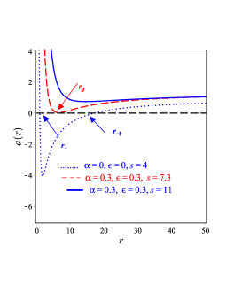
Hence, in order to conclude on the stability of motion around the obtained black-hole solutions, for the case in the above expressions we insert and from (III.1),(26), while for the case from (28).
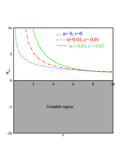
In order to present the above results in a more transparent way, in Fig. 1 we depict the behavior of for various choices of the model parameters, for the two cases and separately. Note that for we always obtain stability of motion as expected, while for we find potentially unstable regions.
V Thermodynamics
In this section we perform an analysis of the thermodynamic properties of the obtained black-hole solutions. Since the nature of the solutions and especially their thermodynamic features change for and , in the following we examine the two cases separately.
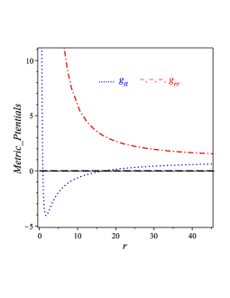
V.1 Thermodynamics of the black hole solution with
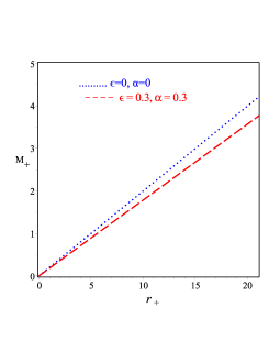
We start by investigating the black-hole solution of the case given in (III.1),(26). In the left graph of Fig. 2 we display the metric potentials and . As we can see, may exhibit two horizons while does not. In the right graph of Fig. 2 we focus on , in order to make more transparent the behavior of its possible two horizons, acquired by solving , namely which denotes the inner Cauchy horizon of the black hole and which is the outer event horizon. In particular, for small values, namely small deviations from general relativity, we obtain two horizons, however as increases there is a specific value in which the two horizons become degenerate (), while for larger values the horizon disappears and the central singularity becomes a naked one. This is a known feature of torsional gravity, namely for some regions of the parameter space naked singularities appear Gonzalez et al. (2012); Capozziello et al. (2013); Nashed and Saridakis (2019). Finally, let us calculate the total mass contained within the event horizon . We find the mass-radius expression as
| (50) |
where is given by Eq. (III.3) for in place of .
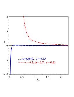
We proceed by examining the temperature. The Hawking black-hole temperature is defined as Sheykhi (2012, 2010); Hendi et al. (2010); Sheykhi et al. (2010)
| (51) |
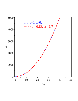
with the event horizon, which satisfies . Additionally, in the framework of gravity, the black-hole entropy is given by Miao et al. (2011); Cognola et al. (2011); Zheng and Yang (2018)
| (52) |
where is the area. Inserting the form (17) and the solution (III.1),(26) into the above definitions we find
| (53) |
and
| (54) |
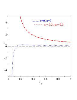
These expressions indicate that for we recover the standard general-relativity temperature and entropy. In Fig. 3 we depict the temperature and entropy versus the horizon, for various values of the model parameters. As we can see the entropy is always positive and exhibits a quadratic behavior, while the temperature is always positive when but for vanishing it is positive only for .
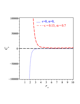
We now focus on the heat capacity, which is a crucial quantity concerning the thermodynamic stability Nashed (2003); Myung (2011, 2013), since our perturbative approach to the black-hole solution allows for an easy calculation. The heat capacity at the event horizon is defined as Nouicer (2007); Dymnikova and Korpusik (2011); Chamblin et al. (1999):
| (55) |
and positive heat capacity implies thermodynamic stability. Substituting (50) and (53) into (55) we obtain the heat capacity as
| (56) |
Expression (56) implies that does not diverge and thus we do not have a second-order phase transition. In the left graph of Fig. 4 we depict as a function of the horizon. As we can see, in the case we have due to the negative derivative of the temperature, as expected for the the Reissner Nordström black hole. Nevertheless, for we obtain positive heat capacity. This is one of the main results of the present work, namely that modifications improve the thermodynamic stability. Note that this is not the case in other gravitational modifications, since for instance in gravity the heat capacity is positive only conditionally Elizalde et al. (2020); Nashed and Saridakis (2020); Nashed and Nojiri (2020).
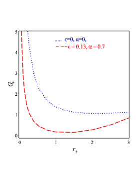
We close this subsection by the examination of the Gibb’s free energy. In terms of the the mass, temperature and entropy at the event horizon this is defined as Zheng and Yang (2018); Kim and Kim (2012):
| (57) |
Inserting (50), (53) and (54) into (57), we obtain
| (58) |
In the right graph of Fig. 4 we depict the behavior of Gibb’s free energy. As we observe it is always positive, for both and .
V.2 Thermodynamics of the black hole solution with
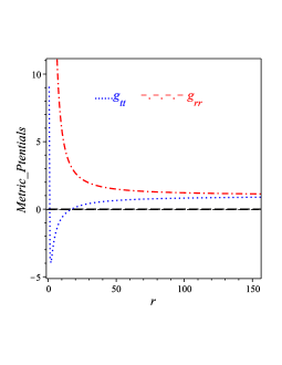
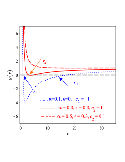
In this subsection we repeat the above thermodynamic analysis in the case of the black hole solution for given in (III.1),(28). In the left graph of Fig. 5 we depict the metric potentials and , and as we observe may exhibit two horizons while does not. In the right graph of Fig. 5 we present . Similarly to the previous subsection, we see that for small values, namely small deviations from general relativity, we obtain two horizons, however as increases there is a specific value in which the two horizons become degenerate (), while for larger values the horizon disappears and the central singularity becomes a naked one. However, the interesting feature is that for the same value, the parameter that quantifies the charge profile also affects the horizon structure, and in particular larger leads to the appearance of the naked singularity.
The mass-radius relation takes the form
| (59) |
and it is plotted in Fig. 6, where we can verify that is always positive.
For the temperature (51) we obtain
| (60) |
Moreover, for the entropy (52) we find
| (61) |
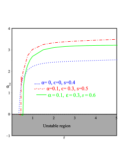
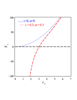
which again for recovers the general relativity result. In Fig. 7 we depict the temperature and entropy versus the horizon, for various values of the model parameters. We mention that in this case both temperature and entropy may acquire negative values, however the entropy, which is always quadratically increasing, is positive when .
For the heat capacity , using (59) and (60), we acquire
| (62) |
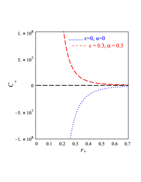
Expression (62) implies that does not diverge and therefore we do not have a second-order phase transition. In the left graph of Fig. 8 we present as a function of the horizon. As we can see, in the case we have due to the negative derivative of the temperature, as expected for the the Reissner Nordström black hole. Nevertheless, for , namely in the case where the correction is switched on, we may obtain positive heat capacity. Finally, for the Gibb’s free energy , using (59), (60) and (61), we find
| (63) |
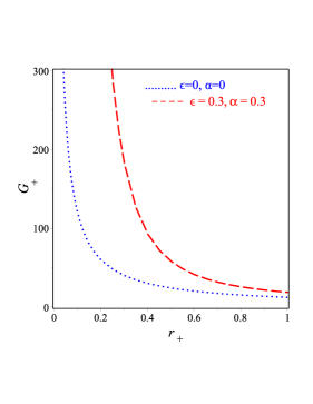
In the right graph of Fig. 8 we present Gibb’s free energy as a function of the horizon. As we can see for both and it is always positive.
VI Conclusions and discussion
We investigated the stability of motion and thermodynamics in the case of spherically symmetric solutions in gravity using the perturbative approach. In particular, we considered small deviations from teleparallel equivalent of general relativity and we extracted charged black hole solutions for two charge profiles, namely with or without a perturbative correction in the charge distribution. Firstly, we examined their asymptotic behavior showing that for large distances they become Minkowski. Then we extracted various torsional and curvature invariants, which revealed the presence of the central singularity as expected. Moreover, we calculated the energy and the mass of the solutions. As we showed, all results recover the general relativity ones in the case where the deviation goes to zero.
As a next step we investigated the stability of motion around the obtained black hole solutions, by extracting and studying the geodesic deviation of a test particle in their gravitational field. Assuming a secular orbit, we extracted the corresponding stability of motion condition in terms of the metric potentials. As we saw, in the case where the perturbative correction to the charge profile is absent the solution is always stable, however in the case where it is present we obtained unstable regimes in the parameter space.
Additionally, we performed a detailed analysis of the thermodynamic properties of the black hole solutions. In particular, we extracted the inner (Cauchy) and outer (event) horizons, the mass profile, the temperature, the entropy, the heat capacity and the Gibb’s free energy. As we showed, for small values, namely small deviations from general relativity, we obtain the two horizons, however as increases there is a specific value in which the two horizons become degenerate, and for larger values the horizon disappears and the central singularity becomes a naked one, a known feature of torsional gravity. Furthermore, we saw that for the same value, the parameter that quantifies the charge profile also affects the horizon structure, and in particular larger leads to the appearance of the naked singularity.
Concerning the temperature and entropy, we showed that although there are regimes in which they become negative, for they are always positive definite. Concerning the heat capacity we saw that it does not diverge and thus we do not have a second-order phase transition. However, the most interesting result is that it becomes positive for larger deviations from general relativity, which shows that modifications improve the thermodynamic stability, which is not the case in other gravitational modifications. Finally, for the Gibb’s free energy, we showed that it is always positive, for all torsional additions and for both charge-profile cases.
In summary, the present work indicates that torsional modification of gravity may have an advantage comparing to other gravitational modification classes, when stability issues are raised, which may serve as an additional motivation for the corresponding investigations. One particular interesting issue is to investigate in detail whether torsional modified gravity leads to smoother (weaker) central singularities comparing to general relativity or curvature modified gravity. This issue will be the focus of interest of a separate project.
References
- Saridakis et al. (2021) E. N. Saridakis et al. (CANTATA) (2021), eprint 2105.12582.
- Stelle (1977) K. S. Stelle, Phys. Rev. D 16, 953 (1977).
- Addazi et al. (2021) A. Addazi, Prog. Part. Nucl. Phys., 103948 (2022).
- Capozziello and De Laurentis (2011) S. Capozziello and M. De Laurentis, Phys. Rept. 509, 167 (2011), eprint 1108.6266.
- Unzicker and Case (2005) A. Unzicker and T. Case (2005), eprint physics/0503046.
- Aldrovandi and Pereira (2013) R. Aldrovandi and J. G. Pereira, Teleparallel Gravity: An Introduction (Springer, 2013), ISBN 978-94-007-5142-2, 978-94-007-5143-9.
- Shirafuji and Nashed (1997) T. Shirafuji and G. G. L. Nashed, Prog. Theor. Phys. 98, 1355 (1997), eprint gr-qc/9711010.
- Maluf (2013) J. W. Maluf, Annalen Phys. 525, 339 (2013), eprint 1303.3897.
- Cai et al. (2016) Y.-F. Cai, S. Capozziello, M. De Laurentis, and E. N. Saridakis, Rept. Prog. Phys. 79, 106901 (2016), eprint 1511.07586.
- Bengochea and Ferraro (2009) G. R. Bengochea and R. Ferraro, Phys. Rev. D 79, 124019 (2009), eprint 0812.1205.
- Linder (2010) E. V. Linder, Phys. Rev. D81, 127301 (2010), eprint 1005.3039.
- Kofinas and Saridakis (2014) G. Kofinas and E. N. Saridakis, Phys. Rev. D 90, 084044 (2014), eprint 1404.2249.
- Bahamonde et al. (2015) S. Bahamonde, C. G. Böhmer, and M. Wright, Phys. Rev. D 92, 104042 (2015), eprint 1508.05120.
- Karpathopoulos et al. (2018) L. Karpathopoulos, S. Basilakos, G. Leon, A. Paliathanasis, and M. Tsamparlis, Gen. Rel. Grav. 50, 79 (2018), eprint 1709.02197.
- Boehmer and Jensko (2021) C. G. Boehmer and E. Jensko, Phys. Rev. D 104, 024010 (2021), eprint 2103.15906.
- Geng et al. (2011) C.-Q. Geng, C.-C. Lee, E. N. Saridakis, and Y.-P. Wu, Phys. Lett. B 704, 384 (2011), eprint 1109.1092.
- Hohmann et al. (2018a) M. Hohmann, L. Järv, and U. Ualikhanova, Phys. Rev. D 97, 104011 (2018a), eprint 1801.05786.
- Bahamonde et al. (2019a) S. Bahamonde, K. F. Dialektopoulos, and J. Levi Said, Phys. Rev. D 100, 064018 (2019a), eprint 1904.10791.
- Zheng and Huang (2011) R. Zheng and Q.-G. Huang, JCAP 03, 002 (2011), eprint 1010.3512.
- El Hanafy and Nashed (2016a) W. El Hanafy and G. G. L. Nashed, Astrophys. Space Sci. 361, 68 (2016a), eprint 1507.07377.
- Bamba et al. (2011) K. Bamba, C.-Q. Geng, C.-C. Lee, and L.-W. Luo, JCAP 01, 021 (2011), eprint 1011.0508.
- Capozziello et al. (2011) S. Capozziello, V. F. Cardone, H. Farajollahi, and A. Ravanpak, Phys. Rev. D 84, 043527 (2011), eprint 1108.2789.
- Wei et al. (2012) H. Wei, X.-J. Guo, and L.-F. Wang, Phys. Lett. B 707, 298 (2012), eprint 1112.2270.
- Amorós et al. (2013) J. Amorós, J. de Haro, and S. D. Odintsov, Phys. Rev. D 87, 104037 (2013), eprint 1305.2344.
- Otalora (2013) G. Otalora, Phys. Rev. D 88, 063505 (2013), eprint 1305.5896.
- Bamba et al. (2013) K. Bamba, S. D. Odintsov, and D. Sáez-Gómez, Phys. Rev. D 88, 084042 (2013), eprint 1308.5789.
- Li et al. (2013) J.-T. Li, C.-C. Lee, and C.-Q. Geng, Eur. Phys. J. C 73, 2315 (2013), eprint 1302.2688.
- Malekjani et al. (2017) M. Malekjani, N. Haidari, and S. Basilakos, Mon. Not. Roy. Astron. Soc. 466, 3488 (2017), eprint 1609.01964.
- Farrugia and Levi Said (2016) G. Farrugia and J. Levi Said, Phys. Rev. D 94, 124054 (2016), eprint 1701.00134.
- Nashed (2014a) G. G. L. Nashed, EPL 105, 10001 (2014a), eprint 1501.00974.
- Saridakis (2017) E. N. Saridakis, in 14th Marcel Grossmann Meeting (2017), vol. 2, pp. 1135–1140.
- Qi et al. (2017) J.-Z. Qi, S. Cao, M. Biesiada, X. Zheng, and H. Zhu, Eur. Phys. J. C 77, 502 (2017), eprint 1708.08603.
- Cai et al. (2018) Y.-F. Cai, C. Li, E. N. Saridakis, and L. Xue, Phys. Rev. D 97, 103513 (2018), eprint 1801.05827.
- Abedi et al. (2018) H. Abedi, S. Capozziello, R. D’Agostino, and O. Luongo, Phys. Rev. D 97, 084008 (2018), eprint 1803.07171.
- El-Zant et al. (2019) A. El-Zant, W. El Hanafy, and S. Elgammal, Astrophys. J. 871, 210 (2019), eprint 1809.09390.
- Anagnostopoulos et al. (2019) F. K. Anagnostopoulos, S. Basilakos, and E. N. Saridakis, Phys. Rev. D 100, 083517 (2019), eprint 1907.07533.
- Cai et al. (2020) Y.-F. Cai, M. Khurshudyan, and E. N. Saridakis, Astrophys. J. 888, 62 (2020), eprint 1907.10813.
- Yan et al. (2020) S.-F. Yan, P. Zhang, J.-W. Chen, X.-Z. Zhang, Y.-F. Cai, and E. N. Saridakis, Phys. Rev. D 101, 121301 (2020), eprint 1909.06388.
- Awad et al. (2018) A. Awad, W. El Hanafy, G. G. L. Nashed, S. D. Odintsov, and V. K. Oikonomou, JCAP 1807, 026 (2018), eprint 1710.00682.
- El Hanafy and Nashed (2019) W. El Hanafy and G. G. L. Nashed, Phys. Rev. D 100, 083535 (2019), eprint 1910.04160.
- Wang and Mota (2020) D. Wang and D. Mota, Phys. Rev. D 102, 063530 (2020), eprint 2003.10095.
- El Hanafy and Saridakis (2021) W. El Hanafy and E. N. Saridakis, JCAP 09, 019 (2021), eprint 2011.15070.
- Nashed (2010) G. G. L. Nashed, Chin. Phys. p. 020401 (2010), eprint 0910.5124.
- Hashim et al. (2021) M. Hashim, W. El Hanafy, A. Golovnev, and A. A. El-Zant, JCAP 07, 052 (2021), eprint 2010.14964.
- Ren et al. (2021a) X. Ren, T. H. T. Wong, Y.-F. Cai, and E. N. Saridakis, Phys. Dark Univ. 32, 100812 (2021a), eprint 2103.01260.
- Boehmer et al. (2011) C. G. Boehmer, A. Mussa, and N. Tamanini, Class. Quant. Grav. 28, 245020 (2011), eprint 1107.4455.
- Gonzalez et al. (2012) P. A. Gonzalez, E. N. Saridakis, and Y. Vasquez, JHEP 07, 053 (2012), eprint 1110.4024.
- Capozziello et al. (2013) S. Capozziello, P. A. Gonzalez, E. N. Saridakis, and Y. Vasquez, JHEP 02, 039 (2013), eprint 1210.1098.
- Ferraro and Fiorini (2011) R. Ferraro and F. Fiorini, Phys. Rev. D 84, 083518 (2011), eprint 1109.4209.
- Wang (2011) T. Wang, Phys. Rev. D 84, 024042 (2011), eprint 1102.4410.
- Atazadeh and Mousavi (2013) K. Atazadeh and M. Mousavi, Eur. Phys. J. C 73, 2272 (2013), eprint 1212.3764.
- El Hanafy and Nashed (2016b) W. El Hanafy and G. G. L. Nashed, Astrophys. Space Sci. 361, 68 (2016b), eprint 1507.07377.
- Rodrigues et al. (2013) M. E. Rodrigues, M. J. S. Houndjo, J. Tossa, D. Momeni, and R. Myrzakulov, JCAP 11, 024 (2013), eprint 1306.2280.
- Nashed (2013a) G. G. L. Nashed, Phys. Rev. D 88, 104034 (2013a), eprint 1311.3131.
- Nashed (2014b) G. G. L. Nashed, Adv. High Energy Phys. 2014, 830109 (2014b).
- Junior et al. (2015) E. L. B. Junior, M. E. Rodrigues, and M. J. S. Houndjo, JCAP 10, 060 (2015), eprint 1503.07857.
- Kofinas et al. (2015) G. Kofinas, E. Papantonopoulos, and E. N. Saridakis, Phys. Rev. D 91, 104034 (2015), eprint 1501.00365.
- Das et al. (2015) A. Das, F. Rahaman, B. K. Guha, and S. Ray, Astrophys. Space Sci. 358, 36 (2015), eprint 1507.04959.
- Awad and Nashed (2017) A. Awad and G. Nashed, JCAP 02, 046 (2017), eprint 1701.06899.
- Nashed (2018) G. G. L. Nashed, Int. J. Mod. Phys. D 27, 1850074 (2018).
- Rani et al. (2016) S. Rani, A. Jawad, and M. B. Amin, Commun. Theor. Phys. 66, 411 (2016).
- Rodrigues and Junior (2018) M. E. Rodrigues and E. L. B. Junior, Astrophys. Space Sci. 363, 43 (2018), eprint 1606.04918.
- Mai and Lu (2017) Z.-F. Mai and H. Lu, Phys. Rev. D 95, 124024 (2017), eprint 1704.05919.
- Newton Singh et al. (2019) K. Newton Singh, F. Rahaman, and A. Banerjee, Phys. Rev. D 100, 084023 (2019), eprint 1909.10882.
- Nashed and Capozziello (2020) G. G. L. Nashed and S. Capozziello, Eur. Phys. J. C 80, 969 (2020), eprint 2010.06355.
- Bhatti (2018) M. Z. Bhatti, Eur. Phys. J. Plus 133, 431 (2018).
- Ashraf et al. (2020) A. Ashraf, Z. Zhang, A. Ditta, and G. Mustafa, Annals Phys. 422, 168322 (2020).
- Ditta et al. (2021) A. Ditta, M. Ahmad, I. Hussain, and G. Mustafa, Chin. Phys. C 45, 045102 (2021).
- Ren et al. (2021b) X. Ren, Y. Zhao, E. N. Saridakis, and Y.-F. Cai, JCAP 10, 062 (2021b), eprint 2105.04578.
- Ferraro and Fiorini (2011) R. Ferraro and F. Fiorini, Phys. Rev. D 84, 083518 (2011), eprint 1109.4209.
- Nashed (2013b) G. G. L. Nashed, Gen. Rel. Grav. 45, 1887 (2013b), eprint 1502.05219.
- Nashed (2013) G. G. L. Nashed, Phys. Rev. D 88, 104034 (2013), eprint 1311.3131.
- Nashed (2019) G. Nashed, Int. J. Mod. Phys. D28, 1950158 (2019).
- Nashed and Saridakis (2019) G. G. L. Nashed and E. N. Saridakis, Class. Quant. Grav. 36, 135005 (2019), eprint 1811.03658.
- Awad et al. (2017) A. M. Awad, S. Capozziello, and G. G. L. Nashed, JHEP 07, 136 (2017), eprint 1706.01773.
- Nashed and El Hanafy (2017) G. G. L. Nashed and W. El Hanafy, Eur. Phys. J. C 77, 90 (2017), eprint 1612.05106.
- Paliathanasis et al. (2014) A. Paliathanasis, S. Basilakos, E. N. Saridakis, S. Capozziello, K. Atazadeh, F. Darabi, and M. Tsamparlis, Phys. Rev. D 89, 104042 (2014), eprint 1402.5935.
- DeBenedictis and Ilijic (2016) A. DeBenedictis and S. Ilijic, Phys. Rev. D 94, 124025 (2016), eprint 1609.07465.
- Bahamonde et al. (2020) S. Bahamonde, J. Levi Said, and M. Zubair, JCAP 10, 024 (2020), eprint 2006.06750.
- Bahamonde et al. (2019b) S. Bahamonde, K. Flathmann, and C. Pfeifer, Phys. Rev. D 100, 084064 (2019b), eprint 1907.10858.
- Ruggiero and Radicella (2015) M. L. Ruggiero and N. Radicella, Phys. Rev. D 91, 104014 (2015), eprint 1501.02198.
- Nashed (2021) G. G. L. Nashed, Class. Quant. Grav. 38, 125004 (2021), eprint 2105.05688.
- Böhmer and Fiorini (2019) C. G. Böhmer and F. Fiorini, Class. Quant. Grav. 36, 12LT01 (2019), eprint 1901.02965.
- Böhmer and Fiorini (2020) C. G. Böhmer and F. Fiorini, Class. Quant. Grav. 37, 185002 (2020), eprint 2005.11843.
- Plebański (1970) J. Plebański, Lectures on non-linear electrodynamics (NORDITA, 1970), URL https://books.google.com.eg/books?id=zEZUAAAAYAAJ.
- Krššák and Saridakis (2016) M. Krššák and E. N. Saridakis, Class. Quant. Grav. 33, 115009 (2016), eprint 1510.08432.
- Golovnev et al. (2017) A. Golovnev, T. Koivisto, and M. Sandstad, Class. Quant. Grav. 34, 145013 (2017), eprint 1701.06271.
- Hohmann et al. (2018b) M. Hohmann, L. Järv, M. Krššák, and C. Pfeifer, Phys. Rev. D97, 104042 (2018b), eprint 1711.09930.
- Bahamonde et al. (2019c) S. Bahamonde, K. Flathmann, and C. Pfeifer, Physical Review D 100 (2019c), ISSN 2470-0029, URL http://dx.doi.org/10.1103/PhysRevD.100.084064.
- Nesseris et al. (2013) S. Nesseris, S. Basilakos, E. N. Saridakis, and L. Perivolaropoulos, Phys. Rev. D 88, 103010 (2013), eprint 1308.6142.
- Nunes et al. (2016) R. C. Nunes, S. Pan, and E. N. Saridakis, JCAP 08, 011 (2016), eprint 1606.04359.
- Li et al. (2018) C. Li, Y. Cai, Y.-F. Cai, and E. N. Saridakis, JCAP 10, 001 (2018), eprint 1803.09818.
- Ulhoa and Spaniol (2013) S. C. Ulhoa and E. P. Spaniol, International Journal of Modern Physics D 22, 1350069 (2013), ISSN 1793-6594, URL http://dx.doi.org/10.1142/S0218271813500697.
- Maluf et al. (2002) J. W. Maluf, J. F. da Rocha-Neto, T. M. L. Toríbio, and K. H. Castello-Branco, Phys. Rev. D 65, 124001 (2002), URL https://link.aps.org/doi/10.1103/PhysRevD.65.124001.
- Nashed and Shirafuji (2007) G. G. L. Nashed and T. Shirafuji, International Journal of Modern Physics D 16, 65–79 (2007), ISSN 1793-6594, URL http://dx.doi.org/10.1142/S0218271807009310.
- D’Inverno (1992) R. A. D’Inverno, Introducing Einstein’s relativity (1992).
- Sheykhi (2012) A. Sheykhi, Phys. Rev. D 86, 024013 (2012), URL https://link.aps.org/doi/10.1103/PhysRevD.86.024013.
- Sheykhi (2010) A. Sheykhi, Eur. Phys. J. C69, 265 (2010), eprint 1012.0383.
- Hendi et al. (2010) S. H. Hendi, A. Sheykhi, and M. H. Dehghani, Eur. Phys. J. C70, 703 (2010), eprint 1002.0202.
- Sheykhi et al. (2010) A. Sheykhi, M. H. Dehghani, and S. H. Hendi, Phys. Rev. D 81, 084040 (2010), URL https://link.aps.org/doi/10.1103/PhysRevD.81.084040.
- Miao et al. (2011) R.-X. Miao, M. Li, and Y.-G. Miao, JCAP 11, 033 (2011), eprint 1107.0515.
- Cognola et al. (2011) G. Cognola, O. Gorbunova, L. Sebastiani, and S. Zerbini, Phys. Rev. D 84, 023515 (2011), URL https://link.aps.org/doi/10.1103/PhysRevD.84.023515.
- Zheng and Yang (2018) Y. Zheng and R.-J. Yang, Eur. Phys. J. C78, 682 (2018), eprint 1806.09858.
- Nashed (2003) G. G. L. Nashed, Chaos Solitons Fractals 15, 841 (2003), eprint gr-qc/0301008.
- Myung (2011) Y. S. Myung, Physical Review D 84 (2011), ISSN 1550-2368, URL http://dx.doi.org/10.1103/PhysRevD.84.024048.
- Myung (2013) Y. S. Myung, Phys. Rev. D 88, 104017 (2013), eprint 1309.3346.
- Nouicer (2007) K. Nouicer, Class. Quant. Grav. 24, 5917 (2007), eprint 0706.2749.
- Dymnikova and Korpusik (2011) I. Dymnikova and M. Korpusik, Entropy 13, 1967 (2011), ISSN 1099-4300, URL http://www.mdpi.com/1099-4300/13/12/1967.
- Chamblin et al. (1999) A. Chamblin, R. Emparan, C. V. Johnson, and R. C. Myers, Phys. Rev. D60, 064018 (1999), eprint hep-th/9902170.
- Elizalde et al. (2020) E. Elizalde, G. G. L. Nashed, S. Nojiri, and S. D. Odintsov, Eur. Phys. J. C 80, 109 (2020), eprint 2001.11357.
- Nashed and Saridakis (2020) G. G. L. Nashed and E. N. Saridakis, Phys. Rev. D 102, 124072 (2020), eprint 2010.10422.
- Nashed and Nojiri (2020) G. G. L. Nashed and S. Nojiri, Phys. Rev. D 102, 124022 (2020), eprint 2012.05711.
- Kim and Kim (2012) W. Kim and Y. Kim, Phys. Lett. B718, 687 (2012), eprint 1207.5318.