Optimal control of families of quantum gates

Abstract

Quantum Optimal Control (QOC) enables the realization of accurate operations, such as quantum gates, and support the development of quantum technologies. To date, many QOC frameworks have been developed but those remain only naturally suited to optimize a single targeted operation at a time. We extend this concept to optimal control with a continuous family of targets, and demonstrate that an optimization based on neural networks can find families of time-dependent Hamiltonians that realize desired classes of quantum gates in minimal time.

After concerted efforts in the development of synthetic quantum systems we have access to a variety of systems with sufficiently long coherence time to perform a series of coherent operations. In the community’s effort to turn such systems into technological applications, Quantum Optimal Control (QOC) [1, 2] helps to increase the precision and rate of desired operations. Common problems successfully addressed by means of QOC include the realization of quantum gates or entangled states in few-body or many-body systems [3, 4, 5, 6, 7, 8, 9, 10, 11] and the refinement of metrology protocols [12, 13].

Current tasks of optimal control are mostly focused on the realization of a single target operation, such as the preparation of one specific state or the implementation of one specific gate. Yet, as quantum technologies mature, it becomes important to enlarge the range of operations which can be accurately implemented on a device. For instance, in the context of Noisy-Intermediate Scale Quantum (NISQ) devices [14], augmenting the set of available elementary gates allows for more compact compilation of quantum circuits, i.e., their decomposition into these elementary gates. Already the inclusion of continuous families of two-qubit gates to a typical gate-set, composed of single-qubit rotations and a two-qubit entangling gate, can lead to a significant reduction in gate count [15, 16, 17]. This, in turn, opens the possibility to run more expressive computations before the onset of decoherence, a key limitation in current technology. That is, the ability to implement a broader range of optimized operations has the potential to substantially increase the utility of current quantum hardware.

Despite the many flavours of QOC frameworks that have been proposed (e.g., [18, 19, 20, 21, 22, 23, 24, 25, 26, 27, 28]), it remains the case that current methodologies are only naturally suited to consider a single control task at a time. We thus aim at lifting the original scope of QOC from the control of a single target operation to the control of continuous families of targets. This is achieved with a neural-network (NN) modelling the dependency between Hamiltonians to be engineered and control tasks to be solved. Efficient training of the framework by means of gradient-descent is facilitated by recent advances in the field of automatic-differentiation [29]. Such framework, dubbed family-control, is sketched in Fig. 1 and is now explained in detail.

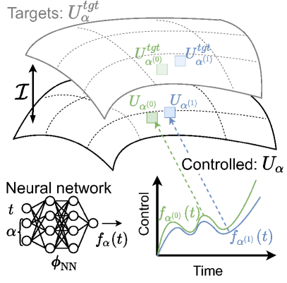
Figure 1: Optimal control of a continuous family of target gates $U^{tgt}_{\alpha}$ indexed by the target parameter $\alpha$ which can be either a scalar or a vector. The time-dependent controls $f_{\alpha}(t)$ which now also depend on $\alpha$ are modeled by a neural network (NN). This NN effectively parameterizes a continuous family of controlled gates $U_{\alpha}$ where each point corresponds to the propagator obtained by evolving the system in time (dashed arrows) under the controls produced by the NN (illustrated for two set of target parameters $\alpha^{(0)}$ and $\alpha^{(1)}$). Training of the framework consists in optimizing the weights of the NN, denoted $\phi_{NN}$, such that the deviation $\mathcal{I}$ between the controlled and target families of operations is minimized.

Typically, the central task in QOC is the identification of the time-dependent Hamiltonian $H(t)$ that induces a propagator $U(t)$ with desired properties. This is formulated in terms of a cost functional $\mathcal{I}(H(t))$ that is to be minimized. A common example would be the task of realizing a target controlled–not gate $U^{tgt}=|0\rangle\langle 0|\otimes I+|1\rangle\langle 1|\otimes\sigma_{x}$ at a given time $T$, with the cost $\mathcal{I}(H(t))=||U(T)-U^{tgt}||$ being a measure of the deviation between the controlled and target propagators. A corresponding task of family-control could be the realization of the family of target gates $U^{tgt}_{\alpha}=|0\rangle\langle 0|\otimes I+|1\rangle\langle 1|\otimes\exp(-i\alpha\sigma_{x})$ with a variable angle $\alpha$. In this case, the overall task to be solved would be the identification of a continuum of Hamiltonians $H_{\alpha}(t)$, parameterized by the angle $\alpha$, such that any of the propagators $U_{\alpha}=U_{\alpha}(t=T)$ induced by $H_{\alpha}(t)$ approximates the gate $U^{tgt}_{\alpha}$ as well as possible at $t=T$. The corresponding functional would thus become $\mathcal{I}(H_{\alpha}(t))=\langle||U_{\alpha}-U^{tgt}_{\alpha}||\rangle_{\alpha}$ with an average over $\alpha$.

The general formulation of such a family-control problem can be given in terms of the individual costs $\mathcal{I}_{\alpha}(H_{\alpha}(t))$, where the target parameter $\alpha$ can be a single scalar or a vector. The overall task to be solved is the identification of the continuum of time-dependent Hamiltonians $H_{\alpha}(t)$ that minimizes the averaged cost $\mathcal{I}=\langle\mathcal{I}_{\alpha}(H_{\alpha}(t))\rangle_{\alpha}$.

In principle, this can be addressed in terms of several control problems to be solved separately for a discretized set of target values $\{\alpha^{(i)}\}$,and, an additional step of interpolation for any new target with $\alpha\notin\{\alpha^{(i)}\}$. Hardly any control problem, however, has a unique solution, or at least a unique solution that can be found in practice. That is, there is no guarantee for two Hamiltonians $H_{\alpha^{(1)}}$ and $H_{\alpha^{(1)}}$ identified as optimal for similar values of $\alpha^{(1)}$ and $\alpha^{(2)}$, to be themselves similar. Any attempt to find an optimal Hamiltonian for a value of $\alpha$ between $\alpha^{(1)}$ and $\alpha^{(2)}$ in terms of an interpolation between $H_{\alpha^{(1)}}$ and $H_{\alpha^{(2)}}$ can thus result in a Hamiltonian that utterly fails to realize the desired task. In order to avoid this issue, it is desirable to require $H_{\alpha}$ to depend smoothly on $\alpha$. Such requirement can be realized by means of an appropriate parameterization of the dependence of $H_{\alpha}(t)$ on both $\alpha$ and $t$. Given that neural networks (NNs) provide the flexible structure to approximate multivariate continuous functions up to any desired precision [30], these are deemed ideally suited for the task at hand.

Time-dependence in a Hamiltonian is typically realized in terms of temporally modulated electro-magnetic fields that appear as one or several control functions $f_{\alpha}(t)$ in the Hamiltonian. The scope of the NN is thus to model these functions. To this intent, the parameters $\alpha$ and the time $t$ are taken to be the inputs of the NN, and the control values $f_{\alpha}(t)$ its outputs. An example of such a NN is illustrated in Fig. 1 for the case of two–dimensional parameters $\alpha$ and a single control function $f_{\alpha}(t)$; it is readily adapted to arbitrary dimensions of the parameters and number of controls by varying the sizes of the inputs and outputs accordingly.

The optimization – i.e., training of the neural network – can be achieved with a variety of techniques, but gradient-descent training has the advantage of simplicity and scalability to high-dimensional problems. Since the propagators $U_{\alpha}$ induced by the Hamiltonians $H_{\alpha}$ typically need to be constructed numerically, efficient means to take derivatives with respect to the control functions $f_{\alpha}(t)$ are essential. Recent advances in the field of automatic differentiation [29] give access to efficient differentiation over numerical solvers of differential equations. This allows to combine seamlessly gradients over the evolution of the system and over the weights of the NN. Finally, even though the evaluation of the averaged cost $\mathcal{I}$ would always be based on a sum over discrete values of $\alpha$ rather than a proper integral, the output of the neural network is still continuous in $\alpha$, and choosing different random sampling points at each step in the training process avoids finding solutions with artefacts resulting from the sampling. Implementation details can be found in Sec. I of Supp. Matt.

The following discussion exemplifies the framework sketched so far, with the realization of quantum gates induced by the $n$–qubit Hamiltonian

$$\mathcal{H}_{\alpha}(t)=\sum_{i<j=1}^{n}f_{\alpha}^{ij}\sigma_{x}^{(i)}\sigma_{x}^{(j)}+\sum_{i=1}^{n}f_{\alpha}^{iy}\sigma_{y}^{(i)}+f_{\alpha}^{iz}\sigma_{z}^{(i)}\ ,$$ (1)

with pairwise $\sigma_{x}\sigma_{x}$ interactions, single-qubit Pauli $\sigma_{y}$ and $\sigma_{z}$ terms, and time-dependent control functions $f_{\alpha}^{ij}(t)$, $f_{\alpha}^{iy}(t)$ and $f_{\alpha}^{iz}(t)$. The Hamiltonian is sufficiently general so that any desired $n$–qubit unitary can be realized [31], but bounded control amplitudes $\{f_{\alpha}^{ij},f_{\alpha}^{iy},f_{\alpha}^{iz}\}\in[-1,1]$ typically result in a finite minimal time required to realize a given unitary. Deviations between controlled and target gates are characterized in terms of the gate infidelities

$${\cal I}_{\alpha}(H_{\alpha}(t))=1-\frac{1}{2^{n}}\left|\mbox{Tr}\ [U_{\alpha}^{\dagger}U^{tgt}_{\alpha}]\right|^{2}$$ (2)

in the subsequent examples.

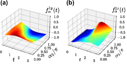
Figure 2: Control of the family of arbitrary single–qubit rotations $U^{1}_{\alpha}$ defined in Eq. (3) with the Hamiltonian given in Eq. (1). The framework is successfully trained to implement any of the target rotations, resulting in an average infidelity of $\bar{\mathcal{I}}=2\times 10^{-4}$ (which is assessed based on new targets that were not seen during training). To visualize the controls produced by the NN, $\alpha_{1}$ and $\alpha_{2}$ are kept fixed to a value of $3\pi/4$ and $\alpha_{3}$ is varied in the range $[0,\pi]$. The amplitudes of the two control fields $f_{\alpha}^{1y}$ (inset a), and $f_{\alpha}^{1z}$ (inset b) produced by the NN are plotted as a function of both the time $t$ and $\alpha_{3}/\pi$.

The basic workings of the present framework can be illustrated with the task of realizing the manifold of single-qubit gates

$$U^{1}_{\alpha}=\exp\left(-i\frac{\alpha_{1}}{2}\sigma_{z}\right)\exp\left(-i\frac{\alpha_{2}}{2}\sigma_{y}\right)\exp\left(-i\frac{\alpha_{3}}{2}\sigma_{z}\right)$$ (3)

for the three-dimensional target parameters $\alpha$ with components $\alpha_{j=1,2,3}\in[0,\pi]$, given the single-qubit version of $\mathcal{H}_{\alpha}(t)$ in Eq. (1) and a fixed gate time $T=\pi$. Here, and in all subsequent examples, the training stage is limited to $400$ iterations, with each iteration corresponding to an average of the gate infidelity in Eq. (2) taken over $128$ values of the parameters $\alpha$ uniformly sampled.

After training, the average gate infidelity $\bar{\cal I}=\langle{\cal I}_{\alpha}\rangle_{\alpha}$ resulting from the controls identified as optimal by the framework, is evaluated on an ensemble of $250$ random values of the parameters $\alpha$. Crucially, this average is taken with respect to new parameter values (that is, corresponding to targets which have not been seen during training), and thus probes the ability of the framework to realize any gates belonging to the targeted family. In this example, the average infidelity is as low as $\bar{\mathcal{I}}=2[3]\times 10^{-4}$, where the number in brackets indicates the standard deviation of the distribution. Fig. 2 depicts the two control functions $f_{\alpha}^{1y}(t)$ and $f_{\alpha}^{1z}(t)$ (insets (a) and (b) respectively) as function of $\alpha_{3}/\pi$ and $t$ for $\alpha_{1}=\alpha_{2}=3\pi/4$, substantiating that the solutions produced by the neural network are indeed well-behaved, continuous functions of both the parameters $\alpha$ and time $t$.

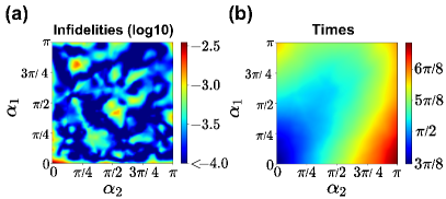
Figure 3: Infidelities and times for the family $U_{\alpha}^{1}$ of rotations. In this example, both the (target-dependent) control functions and times are learnt concurrently. For the sake of visualization, results are plotted for a two-dimensional subset of the three–dimensional family of targets, with fixed parameter $\alpha_{3}=3\pi/4$, and discretized $\alpha_{1},\alpha_{2}\in[0,\pi]$ over a grid of $75\times 75$ regularly spaced points. For each of the corresponding target gates a heat-map indicates the values of the infidelities $\mathcal{I}_{\alpha}$ achieved (inset a, in logarithmic scale) and the control times $T_{\alpha}$ entailed by the framework (inset b).

In addition to an optimization of control functions, the present framework is also well suited to identify a minimal gate time $T$, or even minimal target-dependent gate times $T_{\alpha}$ (Sec. I B of Supp. Matt.). The latter is achieved by introducing a second neural network with the gate time $T_{\alpha}$ as an output. Given the new cost ${\cal I}_{\alpha}+\mu\times T_{\alpha}$ comprised of the gate infidelity and the gate time as a penalty weighted with a scalar factor $\mu>0$, this second neural network can be trained similarly to the case discussed above.

In Fig. 3 are reported the results from such an optimization with a small value $\mu=10^{-2}$ of the weight factor which is suitable to find high-fidelity gates close to the minimally required time. Inset (a) depicts the infidelity ${\cal I}_{\alpha}$ of the resulting gates for $\alpha_{3}=3\pi/4$ as function of $\alpha_{1}$ and $\alpha_{2}$. Typical values are smaller than $10^{-3}$ and the average infidelity with the average taken over all three components of $\alpha$ is $\bar{\cal I}=4[5]\times 10^{-4}$.

Inset (b) depicts the target-dependent minimized gate times, with again a fixed value of $\alpha_{3}=3\pi/4$ but varied $\alpha_{1}$ and $\alpha_{2}$. The shortest gate time is obtained for $\alpha_{1}=\alpha_{2}=0$ (i.e., for the target parameters $\alpha^{(0)}=[0,0,3\pi/4]$) in which case the constant control amplitudes $f_{\alpha^{(0)}}^{1z}(t)=1$ and $f_{\alpha^{(0)}}^{1y}(t)=0$ induce the desired gate $U^{1}_{\alpha^{(0)}}=\exp(-i\frac{3\pi}{8}\sigma_{z})$ after a time $T_{\alpha^{(0)}}=3\pi/8$. The obtained gate times grow with increasing values of $\alpha_{1}$ and $\alpha_{2}$, but always remain below the value of $\pi$ used in the above example.

While the ability to realize single-qubit gates is of substantial practical value, it is certainly not the challenging control problem that helps to demonstrate the actual strength of the framework. This is better achieved in terms of two-qubit and three-qubit gates that are building blocks of quantum algorithms or digital quantum simulations.

Table 1: Control under the Hamiltonian of Eq. (1) of families of $n=2$ and $3$ qubit gates, corresponding to $C=5$ and $9$ control functions to be learnt respectively. For each problem the family of target $U^{tgt}_{\alpha}$ considered and the domain $\chi$ of the target parameters $\alpha$ are reported. Results are provided in terms of the average (and standard deviations in bracket) infidelities $\bar{\mathcal{I}}$, and of the ratio $R$ between the average gate times resulting from a decomposition in terms of elementary gates and the times necessitated by the framework. Additional elements of training the families (vi) and (vii) are provided in the main text.

	$U^{tgt}_{\alpha}$	$\chi$	$\bar{\cal I}[10^{-4}]$	$R$
(i)	$|0\rangle\langle 0|\otimes I+|1\rangle\langle 1|\otimes\exp(-i\alpha_{1}\sigma^{(2)}_{z})$	$[0,\pi]$	$1[1]$	$2.0$
(ii)	$\exp\left(-i\alpha_{1}\sigma^{(1)}_{z}\sigma^{(2)}_{z}\right)$	$[0,\frac{\pi}{2}]$	$0[0]$	$2.0$
(iii)	$|0\rangle\langle 0|\otimes I+|1\rangle\langle 1|\otimes U^{1}_{\alpha}$	$[0,\pi]^{3}$	$3[4]$	$2.1$
(iv)	$\exp(-i\sum_{j\in\{x,y,z\}}\alpha_{j}\sigma_{j}^{(1)}\sigma_{j}^{(2)})$	$[0,\frac{\pi}{2}]^{3}$	$4[4]$	$2.6$
(v)	$\exp(-i\alpha_{1}\sigma_{z}^{(1)}\sigma_{z}^{(2)}\sigma_{z}^{(3)})$	$[0,\frac{\pi}{2}]$	$1[0]$	$4.1$
(vi)	$\exp(-i\sum_{j\in\{x,y,z\}}\alpha_{j}\sigma_{j}^{(1)}\sigma_{j}^{(2)}\sigma_{j}^{(3)})$	$[0,\frac{\pi}{2}]^{3}$	$9[8]$	$>10$
(vii)	$\left(I-|11\rangle\langle 11|\right)\otimes I+|11\rangle\langle 11|\otimes U^{1}_{\alpha}$	$[0,\pi]^{3}$	$6[5]$	$>10$

Table 1 summarizes the results for a few selected families of two- and three-qubit gates with the domain $\chi$ of the parameters $\alpha$ depicted in column $3$ and the obtained average infidelities (in multiples of $10^{-4}$) in column $4$ (further details of the NNs used are reported in Sec. I C of Supp. Matt.). The two-qubit gates $(i)$ to $(iv)$ involve the optimization over $C=5$ control functions, and the three-qubit gates $(v)$ to $(vii)$ involve the optimization over $C=9$ control functions.

Consistently with the previous findings, low infidelities $\bar{\mathcal{I}}<5\times 10^{-4}$ are achieved for any of the families of two-qubit gates (i-iv) and for the one-dimensional family of three-qubit gates (v).

A straightforward application of the above framework to the problems $(vi)$ and $(vii)$ – corresponding to $9$ time-dependent controls to be learnt and $3$-dimensional families to be realized – however results in higher infidelities ($3[2.5]\times 10^{-3}$ for (vi) and $1.7[1.5]\times 10^{-3}$ for (vii)) than in the other cases. Yet, the results of the optimizations contain clear indications towards steps to reach higher fidelities that are now further discussed.

First, the lowest fidelities are systematically obtained for values of $\alpha$ close to the boundary of its admissible domain $\chi$ (as can already be seen in Fig. 3(a)). Enlarging the range of values used for training by $20\%$ resolves this effect. Second, the control functions identified as optimal have general properties that can be exploited to reduce the number of independent functions that need to be learnt. In case (vi), the control solutions discovered by the framework satisfy the relation $f_{\alpha}^{13}=f_{\alpha}^{1z}=f_{\alpha}^{3z}=0$ and in case (vii) $f_{\alpha}^{1z}=f_{\alpha}^{2z}=0$, $f_{\alpha}^{1y}=f_{\alpha}^{2y}$ with also $f_{\alpha}^{13}=f_{\alpha}^{23}$. This indicates that only $6$ and $5$ independent control functions, out of the $9$ possible appearing in Eq. (1), are needed for the cases $(vi)$ and $(vii)$ respectively. The infidelities listed in Table 1, for families $(vi)$ and $(vii)$, result from an optimization with enlarged domain $\chi$ and reduced number of control functions, and their magnitude is comparable to those of the other cases.

While generally the non-uniqueness of solutions of optimal control problems makes it difficult to understand why a solution returned by a specific algorithm does achieve the goal that it is meant to achieve, it seems that the requirement of smooth dependence on the parameters $\alpha$ helps the neural network to identify common features of all control pulses within the family and to avoid unnecessary terms in the Hamiltonian that would obscure its working principle.

Beyond this conceptual benefit and the small infidelities that are achieved, the gain in gate time is also of high practical relevance. Since state-of-the-art implementation of unitaries on quantum devices rely on their decompositions in terms of elementary gates, the times $T^{dec}$ entailed by such decompositions provide well-defined baselines. Given the freedom offered by the controlled Hamiltonian in Eq. (1) these decomposition are performed in terms of the gate-set of rotations generated by the single qubit $\sigma_{y}$ and $\sigma_{z}$ and two-qubit $\sigma_{x}\sigma_{x}$ operators, for which qiskit’s [32] compiling routine is employed with the highest level of optimization available (Sec. II of Supp. Matt.).

Column $5$ of Table 1 depicts the ratio $R$ between the averaged durations $\langle T^{dec}_{\alpha}\rangle_{\alpha}$ obtained with compiled gate circuits and the durations obtained with the present techniques. In all cases there is an improvement of at least a factor of $2$, but, in cases $(vi)$ and $(vii)$, the improvement is substantially larger. This suggests that compilation techniques (i.e., discrete optimizations) struggle with these complex three-qubit gates, whereas the continuous optimization realized in terms of neural networks does not suffer from these limitations.

The ability to accurately control entire families of gates in reduced time, especially for complex gates, highlights the benefits of the present methodology. Given that the automatic differentiation techniques [29], that ensures the efficient training of the framework, can be applied to any system of ordinary differential equations, family-control can find direct application to a broad range of quantum systems, such as superconducting qubits. Since those are non-linear oscillators with a ladder of excited states, further studies would include suppression of leakage to such states. Similarly, trapped ions or opto-mechanical systems with several interacting degrees of freedom pose control problems that can be addressed with the present techniques. Additionally, automatic differentiation has also been extended to the treatment of stochastic differential equations (e.g.,  [33, 34]) such that family-control can even generalize to problems of control with active feedback [35, 36].

While optimal control is traditionally realized in terms of control pulses designed in numerical experiments, fundamental limitations in modelling and simulating the dynamics of composite quantum systems resulted in a shift towards designing control pulses in laboratory experiments [37, 38, 39, 40]. Just like many techniques for individual control targets could be generalized to this setting, also family-control could be trained based exclusively on experimental data, either in situations where gradients can be experimentally estimated [41], or by resorting to gradient-free optimization strategies [42].

Essentially, the methodology that was presented here enables the control of a quantum system in different contexts. In the examples investigated, this context was in one to one correspondence with the target gate to be realized, that is, the overall details of the system under control were kept fixed and only the targets were varied. More generally, the scheme based on NNs allows to tailor controls to be applied to any relevant context variable. For instance, the inputs of the NN could also include intrinsic details of the controlled system (such as varied energy detunings [43] or sizes [44]) or extrinsic (such as environmental heating rates [45] or nearby operations inducing cross-talk [46]). Provided that the effects of these context variables can be simulated and that the corresponding optimal controls are expected to vary continuously with these variables, one would learn to accurately operate a quantum device in very broad situations.

We are indebted to stimulating discussions with Selwyn Simsek. This work is supported through a studentship in the Quantum Systems Engineering Skills and Training Hub at Imperial College London funded by EPSRC (Grant No. EP/P510257/1), and through funding from the QuantERA ERANET Cofund in Quantum Technologies implemented within the European Union’s Horizon 2020 Programme under the project Theory-Blind Quantum Control TheBlinQC and from EPSRC under the grant EP/R044082/1.

References

- Werschnik and Gross [2007] J. Werschnik and E. K. U. Gross, Quantum optimal control theory, J. Phys. B 40, R175 (2007).
- Glaser et al. [2015] S. J. Glaser, U. Boscain, T. Calarco, C. P. Koch, W. Köckenberger, R. Kosloff, I. Kuprov, B. Luy, S. Schirmer, T. Schulte-Herbrüggen, D. Sugny, and F. K. Wilhelm, Training schrödinger’s cat: quantum optimal control, Eur. Phys. J. D 69, 279 (2015).
- Timoney et al. [2008] N. Timoney, V. Elman, S. Glaser, C. Weiss, M. Johanning, W. Neuhauser, and C. Wunderlich, Error-resistant single-qubit gates with trapped ions, Phys. Rev. A 77, 052334 (2008).
- Dolde et al. [2014] F. Dolde, V. Bergholm, Y. Wang, I. Jakobi, B. Naydenov, S. Pezzagna, J. Meijer, F. Jelezko, P. Neumann, T. Schulte-Herbrüggen, J. Biamonte, and J. Wrachtrup, High-fidelity spin entanglement using optimal control, Nature Communications 5, 3371 (2014).
- Choi et al. [2014] T. Choi, S. Debnath, T. A. Manning, C. Figgatt, Z.-X. Gong, L.-M. Duan, and C. Monroe, Optimal quantum control of multimode couplings between trapped ion qubits for scalable entanglement, Phys. Rev. Lett. 112, 190502 (2014).
- Heeres et al. [2017] R. W. Heeres, P. Reinhold, N. Ofek, L. Frunzio, L. Jiang, M. H. Devoret, and R. J. Schoelkopf, Implementing a universal gate set on a logical qubit encoded in an oscillator, Nat. Commun. 8, 94 (2017).
- Schäfer et al. [2018] V. M. Schäfer, C. J. Ballance, K. Thirumalai, L. J. Stephenson, T. G. Ballance, A. M. Steane, and D. M. Lucas, Fast quantum logic gates with trapped-ion qubits, Nature 555, 75 (2018).
- Gong et al. [2019] M. Gong, M.-C. Chen, Y. Zheng, S. Wang, C. Zha, H. Deng, Z. Yan, H. Rong, Y. Wu, S. Li, F. Chen, Y. Zhao, F. Liang, J. Lin, Y. Xu, C. Guo, L. Sun, A. D. Castellano, H. Wang, C. Peng, C.-Y. Lu, X. Zhu, and J.-W. Pan, Genuine 12-qubit entanglement on a superconducting quantum processor, Phys. Rev. Lett. 122, 110501 (2019).
- Levine et al. [2019] H. Levine, A. Keesling, G. Semeghini, A. Omran, T. T. Wang, S. Ebadi, H. Bernien, M. Greiner, V. Vuletić, H. Pichler, and M. D. Lukin, Parallel implementation of high-fidelity multiqubit gates with neutral atoms, Phys. Rev. Lett. 123, 170503 (2019).
- Omran et al. [2019] A. Omran, H. Levine, A. Keesling, G. Semeghini, T. T. Wang, S. Ebadi, H. Bernien, A. S. Zibrov, H. Pichler, S. Choi, J. Cui, M. Rossignolo, P. Rembold, S. Montangero, T. Calarco, M. Endres, M. Greiner, V. Vuletić, and M. D. Lukin, Generation and manipulation of schrödinger cat states in rydberg atom arrays, Science 365, 570 (2019).
- Larrouy et al. [2020] A. Larrouy, S. Patsch, R. Richaud, J.-M. Raimond, M. Brune, C. P. Koch, and S. Gleyzes, Fast navigation in a large hilbert space using quantum optimal control, Phys. Rev. X 10, 021058 (2020).
- Poggiali et al. [2018] F. Poggiali, P. Cappellaro, and N. Fabbri, Optimal control for one-qubit quantum sensing, Phys. Rev. X 8, 021059 (2018).
- Rembold et al. [2020] P. Rembold, N. Oshnik, M. M. Müller, S. Montangero, T. Calarco, and E. Neu, Introduction to quantum optimal control for quantum sensing with nitrogen-vacancy centers in diamond, AVS Quantum Sci. 2, 024701 (2020).
- Preskill [2018] J. Preskill, Quantum Computing in the NISQ era and beyond, Quantum 2, 79 (2018).
- Foxen et al. [2020] B. Foxen, C. Neill, A. Dunsworth, P. Roushan, B. Chiaro, A. Megrant, J. Kelly, Z. Chen, K. Satzinger, R. Barends, F. Arute, K. Arya, R. Babbush, D. Bacon, J. C. Bardin, S. Boixo, D. Buell, B. Burkett, Y. Chen, R. Collins, E. Farhi, A. Fowler, C. Gidney, M. Giustina, R. Graff, M. Harrigan, T. Huang, S. V. Isakov, E. Jeffrey, Z. Jiang, D. Kafri, K. Kechedzhi, P. Klimov, A. Korotkov, F. Kostritsa, D. Landhuis, E. Lucero, J. McClean, M. McEwen, X. Mi, M. Mohseni, J. Y. Mutus, O. Naaman, M. Neeley, M. Niu, A. Petukhov, C. Quintana, N. Rubin, D. Sank, V. Smelyanskiy, A. Vainsencher, T. C. White, Z. Yao, P. Yeh, A. Zalcman, H. Neven, and J. M. Martinis (Google AI Quantum), Demonstrating a continuous set of two-qubit gates for near-term quantum algorithms, Phys. Rev. Lett. 125, 120504 (2020).
- Lacroix et al. [2020] N. Lacroix, C. Hellings, C. K. Andersen, A. Di Paolo, A. Remm, S. Lazar, S. Krinner, G. J. Norris, M. Gabureac, J. Heinsoo, A. Blais, C. Eichler, and A. Wallraff, Improving the performance of deep quantum optimization algorithms with continuous gate sets, PRX Quantum 1, 110304 (2020).
- Abrams et al. [2020] D. M. Abrams, N. Didier, B. R. Johnson, M. P. d. Silva, and C. A. Ryan, Implementation of xy entangling gates with a single calibrated pulse, Nat. Electron. 3, 744 (2020).
- Khaneja et al. [2005] N. Khaneja, T. Reiss, C. Kehlet, T. Schulte-Herbrüggen, and S. J. Glaser, Optimal control of coupled spin dynamics: design of nmr pulse sequences by gradient ascent algorithms, J. Magn. Reson. 172, 296 (2005).
- Caneva et al. [2011] T. Caneva, T. Calarco, and S. Montangero, Chopped random-basis quantum optimization, Phys. Rev. A 84, 022326 (2011).
- Reich et al. [2012] D. M. Reich, M. Ndong, and C. P. Koch, Monotonically convergent optimization in quantum control using krotov’s method, J. Chem. Phys. 136, 104103 (2012).
- Zahedinejad et al. [2015] E. Zahedinejad, J. Ghosh, and B. C. Sanders, High-fidelity single-shot toffoli gate via quantum control, Phys. Rev. Lett. 114, 200502 (2015).
- Li et al. [2017] J. Li, X. Yang, X. Peng, and C.-P. Sun, Hybrid quantum-classical approach to quantum optimal control, Phys. Rev. Lett. 118, 150503 (2017).
- Leung et al. [2017] N. Leung, M. Abdelhafez, J. Koch, and D. Schuster, Speedup for quantum optimal control from automatic differentiation based on graphics processing units, Phys. Rev. A 95, 042318 (2017).
- Machnes et al. [2018] S. Machnes, E. Assémat, D. Tannor, and F. K. Wilhelm, Tunable, flexible, and efficient optimization of control pulses for practical qubits, Phys. Rev. Lett. 120, 150401 (2018).
- Bukov et al. [2018] M. Bukov, A. G. R. Day, D. Sels, P. Weinberg, A. Polkovnikov, and P. Mehta, Reinforcement learning in different phases of quantum control, Phys. Rev. X 8, 031086 (2018).
- Niu et al. [2019] M. Y. Niu, S. Boixo, V. N. Smelyanskiy, and H. Neven, Universal quantum control through deep reinforcement learning, npj Quantum Inf. 5, 33 (2019).
- Sauvage and Mintert [2020] F. Sauvage and F. Mintert, Optimal quantum control with poor statistics, PRX Quantum 1, 020322 (2020).
- Coopmans et al. [2021] L. Coopmans, D. Luo, G. Kells, B. K. Clark, and J. Carrasquilla, Protocol discovery for the quantum control of majoranas by differentiable programming and natural evolution strategies, PRX Quantum 2, 020332 (2021).
- Chen et al. [2018] R. T. Q. Chen, Y. Rubanova, J. Bettencourt, and D. K. Duvenaud, Neural ordinary differential equations, in Adv. Neural Inf. Process. Syst., Vol. 31 (2018).
- Hornik [1991] K. Hornik, Approximation capabilities of multilayer feedforward networks, Neural Networks 4, 251 (1991).
- Schirmer et al. [2001] S. G. Schirmer, H. Fu, and A. I. Solomon, Complete controllability of quantum systems, Phys. Rev. A 63, 063410 (2001).
- collaboration [2021] I. collaboration, Qiskit: An open-source framework for quantum computing (2021).
- Jia and Benson [2019] J. Jia and A. R. Benson, Neural jump stochastic differential equations, in Adv. Neural Inf. Process. Syst., Vol. 32 (2019).
- Rackauckas et al. [2020] C. Rackauckas, Y. Ma, J. Martensen, C. Warner, K. Zubov, R. Supekar, D. Skinner, A. Ramadhan, and A. Edelman, Universal differential equations for scientific machine learning, arXiv preprint (2020).
- Schäfer et al. [2021] F. Schäfer, P. Sekatski, M. Koppenhöfer, C. Bruder, and M. Kloc, Control of stochastic quantum dynamics by differentiable programming, Mach. Learn.: Sci. and Technol. 2, 035004 (2021).
- Porotti et al. [2021] R. Porotti, A. Essig, B. Huard, and F. Marquardt, Deep reinforcement learning for quantum state preparation with weak nonlinear measurements, arXiv preprint (2021).
- Kelly et al. [2014] J. Kelly, R. Barends, B. Campbell, Y. Chen, Z. Chen, B. Chiaro, A. Dunsworth, A. G. Fowler, I.-C. Hoi, E. Jeffrey, A. Megrant, J. Mutus, C. Neill, P. J. J. O’Malley, C. Quintana, P. Roushan, D. Sank, A. Vainsencher, J. Wenner, T. C. White, A. N. Cleland, and J. M. Martinis, Optimal quantum control using randomized benchmarking, Phys. Rev. Lett. 112, 240504 (2014).
- Werninghaus et al. [2021] M. Werninghaus, D. J. Egger, F. Roy, S. Machnes, F. K. Wilhelm, and S. Filipp, Leakage reduction in fast superconducting qubit gates via optimal control, npj Quantum Inf. 7, 14 (2021).
- Greenaway et al. [2021] S. Greenaway, F. Sauvage, K. E. Khosla, and F. Mintert, Efficient assessment of process fidelity, Phys. Rev. Research 3, 033031 (2021).
- Baum et al. [2021] Y. Baum, M. Amico, S. Howell, M. Hush, M. Liuzzi, P. Mundada, T. Merkh, A. R. Carvalho, and M. J. Biercuk, Experimental deep reinforcement learning for error-robust gateset design on a superconducting quantum computer, arXiv preprint (2021).
- Banchi and Crooks [2021] L. Banchi and G. E. Crooks, Measuring Analytic Gradients of General Quantum Evolution with the Stochastic Parameter Shift Rule, Quantum 5, 386 (2021).
- Salimans et al. [2017] T. Salimans, J. Ho, X. Chen, S. Sidor, and I. Sutskever, Evolution strategies as a scalable alternative to reinforcement learning, arXiv preprint (2017).
- Porotti et al. [2019] R. Porotti, D. Tamascelli, M. Restelli, and E. Prati, Coherent transport of quantum states by deep reinforcement learning, Commun. Phys. 2, 61 (2019).
- van Frank et al. [2016] S. van Frank, M. Bonneau, J. Schmiedmayer, S. Hild, C. Gross, M. Cheneau, I. Bloch, T. Pichler, A. Negretti, T. Calarco, and S. Montangero, Optimal control of complex atomic quantum systems, Sci. Rep. 6, 34187 (2016).
- Horn et al. [2018] K. P. Horn, F. Reiter, Y. Lin, D. Leibfried, and C. P. Koch, Quantum optimal control of the dissipative production of a maximally entangled state, New J. Phys. 20, 123010 (2018).
- Winick et al. [2021] A. Winick, J. J. Wallman, and J. Emerson, Simulating and mitigating crosstalk, Phys. Rev. Lett. 126, 230502 (2021).