Is the Hemispheric Asymmetry of Monthly Sunspot Area an Irregular Process with Long-Term Memory?

Abstract

The hemispheric asymmetry of the sunspot cycle is a real feature of the Sun. However, its origin is still not well understood. Here we perform nonlinear time series analysis of the sunspot area (and number) asymmetry to explore its dynamics. By measuring the correlation dimension of the sunspot area asymmetry, we conclude that there is no strange attractor in the data. Further computing Higuchi’s dimension, we conclude that the hemispheric asymmetry is largely governed by stochastic noise. However, the behaviour of Hurst exponent reveals that the time series is not completely determined by a memory-less stochastic noise, rather there is a long-term persistence, which can go beyond two solar cycles. Therefore, our study suggests that the hemispheric asymmetry of the sunspot cycle is predominantly originated due to some irregular process in the solar dynamo. The long-term persistence in the solar cycle asymmetry suggests that the solar magnetic field has some memory in the convection zone.

1 Introduction

The magnetic activity of Sun is not identical in two hemispheres—there is always an asymmetry. This hemispheric asymmetry, also called the north-south asymmetry, has been observed in the photospheric magnetic field (Mordvinov & Kitchatinov, 2004; McIntosh et al., 2013; Mordvinov & Kitchatinov, 2019) as well as in many proxies of the solar activity (Mandal et al., 2017; Goel & Choudhuri, 2009; Norton et al., 2014; Mordvinov et al., 2020). The hemispheric asymmetry is a real feature of the solar cycle and is not an artefact of inaccurate or noisy observations (Carbonell et al., 1993).

Bell (1961) found the evidence of hemispheric asymmetry in the number of major flares and later Bell (1962) found a long-term asymmetry in the sunspot area data during Cycles 8–18. Swinson et al. (1986) found a peak in the northern hemispheric solar activity about two years after sunspot minimum and a 22-years periodicity in the north-south asymmetry. Verma (1987) showed that the northern hemisphere is more active during Cycles 19 and 20. Li et al. (2009) used group sunspot and sunspot area data from 1996 to 2007 to show that the solar activity for cycle 23 is dominant in the southern hemisphere; also see Chowdhury et al. (2013) who extended this study to some part of cycle 24. A well-known sunspot asymmetry was observed during the Maunder minimum. Most of the sunspots were registered in the southern hemisphere (Sokoloff & Nesme-Ribes, 1994).

It is believed that a hydromagnetic dynamo, operating in the solar convection zone, is responsible for the generation and maintenance of the large-scale magnetic field and the cycle of solar activity (Parker, 1955). In the current scenario of the solar dynamo (Karak et al., 2014; Charbonneau, 2020; Hazra, 2021), a toroidal component of the magnetic field is largely generated due to the shearing of the poloidal component by the differential rotation. This toroidal field gives back to the poloidal one due to the decay and dispersal of tilted bipolar magnetic regions (BMRs)— the so-called Babcock–Leighton process and possibly due to the helical convection—the so-called $\alpha$ effect. Meridional circulation and the small-scale convective flow play the role in transporting the magnetic field from the near-surface layer (the location of Babcock–Leighton process) to the deeper convection zone, where the shearing process is efficient, and thus largely regulates the cycle period.

The turbulent nature of the helical convective flow—the main drive of the dynamo—is expected to make the magnetic field unequal in two hemispheres. Thus, a hemispheric asymmetry in the solar magnetic field is unavoidable. Furthermore, the tilts of BMRs, which primarily determines the poloidal field, has a large scatter around Joy’s law (Stenflo & Kosovichev, 2012; Wang et al., 2015; Arlt et al., 2016; Jha et al., 2020). Thus the tilt scatter makes the poloidal magnetic field irregular and asymmetric (Lemerle & Charbonneau, 2017; Karak & Miesch, 2017; Karak, 2020). As the poloidal field is the seed for the toroidal field of the next solar cycle, the asymmetry in the polar field is propagated in the solar cycle (Choudhuri et al., 2007). Dynamo models have shown that when the turbulent diffusion is sufficiently strong, the coupling between two hemispheres tries to diminish the asymmetry introduced in the polar field and thus the asymmetry in the solar cycle may not persist for several cycles (Chatterjee & Choudhuri, 2006; Goel & Choudhuri, 2009; Karak, 2010; Karak & Miesch, 2017). Dynamo models by including scatter in the BMR tilt (Lemerle & Charbonneau, 2017; Karak & Miesch, 2017, 2018) or $\alpha$ term in the poloidal source (Olemskoy & Kitchatinov, 2013; Karak et al., 2018; Hazra & Nandy, 2019) produce hemispheric asymmetry in the magnetic cycle, which in some parameter regimes, are in agreement with observations. Schüssler & Cameron (2018) have shown that the random excitation of the quadrupole mode of dynamo by the stochastic fluctuations in the Babcock–Leighton process can lead to an asymmetry in the observed magnetic field; also see Nepomnyashchikh et al. (2019). Thus, all these previous results motivate us to explore whether the solar hemispheric asymmetry is governed by a low-dimensional chaotic process or stochastic process? Is there any long-term memory in the solar cycle asymmetry?

Nonlinear time series analysis is suitable to answer the above questions. While there exist many such studies for the solar cycle data (e.g., Ostriakov & Usoskin, 1990a; Carbonell et al., 1994; Jevtić et al., 2001; Letellier et al., 2006; Suyal et al., 2009), only a few such studies are performed in the solar cycle asymmetry. Carbonell et al. (1993) computed the correlation dimension of the asymmetry of daily sunspot area during 1874–1989 and did not find any evidence of low-dimensional chaos. By computing the Higuchi’s fractal dimension (Higuchi, 1988) and some nonlinear prediction method for the hemispheric asymmetry of sunspot number during 1947–1984, Watari (1996) concluded that the sunspot number asymmetry is highly irregular and not deterministic chaos.

In the present work, we shall utilize the maximum available sunspot area data (during 1874–2016) of hemispheric asymmetry and apply multiple nonlinear time series techniques to check the inherent nonlinear properties of the system. First, we shall compute the correlation dimension ($D_{2}$) to extract whether the data has any strange attractor in the data and thus this analysis will reveal the existence of any low-dimensional chaos in the underlying system (Grassberger & Procaccia, 1983a). Next, we shall compute a fractal dimension using the method given in Higuchi (1988) which provides a stable estimate of the fractal dimension when the data is more irregular and non-stationary. Higuchi’s dimension will give another independent support of whether the asymmetry data is from a stochastic process or low dimensional chaos. Finally, we shall compute the Hurst exponent (Mandelbrot & Wallis, 1969) to check whether the data has any persistent memory or not. The final conclusion will be presented in Section §6.

2 Observational data

We use the monthly mean sunspot area data during May 1874 – September 2016 obtained from the Royal Greenwich Observatory (RGO) . The RGO data have been the only available record of sunspot area separately in two hemispheres for the longer duration and this is routinely used in many studies of the solar activity (Hathaway, 2015). RGO provides the monthly value of the average (over observed day) of the daily sunspot area in the unit of millionths of a hemisphere and it is evenly spaced. We have also repeated our analyses with the newly available monthly mean hemispheric sunspot number data; §B.

The easy way to measure the asymmetry is to take the difference in the values between two hemispheres (Ballester, J. L. et al., 2005; Chang, 2007), i.e. asymmetry,

$$AS=A_{N}-A_{S},$$ (1)

where $A_{N}$ and $A_{S}$ are the monthly values of the sunspot area in the northern and southern hemispheres, respectively. We note that during solar maxima, the difference becomes large in comparison to the value during minima and this causes a cyclic pattern in the asymmetry; see Figure 1 top panel. Furthermore, if a cycle is strong, then the asymmetry is large and vice versa. Therefore, in the literature (Carbonell et al., 1993; Oliver & Ballester, 1996; Duchlev, 2001; Goel & Choudhuri, 2009; Chowdhury et al., 2013; Priyal et al., 2014), the asymmetry is also measured by normalizing its strength, namely. the normalized asymmetry,

$$AS_{Norm}=\frac{A_{N}-A_{S}}{A_{N}+A_{S}}.$$ (2)

When both $A_{N}$ and $A_{S}$ become equal to zero, we set $AS_{Norm}=0$. We realized that this happens for 15 data points (which is less than $1\%$ of the total data). However, we discussed its effect in Section 4 by replacing these points with interpolated values.

We note that this $AS_{Norm}$ is a different time series than the $AS$; statistics of the data are different ( Table 1). Again this definition of asymmetry is not satisfactory because during the solar minima, when the sunspot area becomes very small and this leads to increase in $AS_{Norm}$; see Figure 1 bottom panel. It was examined in Yi (1992), that dividing the difference of the hemispherical sunspot areas by the total sunspot area results in the appearance of a peak in the power spectrum between 11 and 12 years.

Due to such facts from the literature, where both definitions have been used to measure the solar cycle asymmetry, it becomes necessary to perform analyses of the time series of asymmetry using both the methods that we have discussed above.

Figure 1: Time series of the hemispheric asymmetry of monthly average sunspot area (in unit of millionth of a solar hemisphere) as measured by $AS$ (top) and $AS_{Norm}$ (bottom).

Table 1: Some statistics of the data. Total number of data points used: 1709. Symbols in second to third columns are as follows: $<S>$, the average of the time series; $rms$, the root mean-squared deviation, and $<{\rm PN}>=\sqrt{<S>}$.

Data	$<S>$	$rms$	$<{\rm PN}>/rms$
North	426.79	488.2	0.042
South	409.43	470.1	0.043
AS	17.36	466.9	0.009
ASNorm	0.01	0.6	0.225

3 Methods

To identify the nonlinear properties of the hemispheric asymmetry of sunspot area time series, we shall compute three quantities for $AS$ and $AS_{Norm}$, namely, the Correlation dimension, Higuchi’s dimension, and Hurst exponent. Below, we discuss briefly how to compute these quantities.

3.1 Correlation dimension

First, we shall apply a method of time series analysis to distinguish the random noise in the underlying system from the low dimensional chaos. This method is to measure a fractal dimension of the strange attractor in the system which is popularly known as the correlation dimension ($D_{2}$). The method for obtaining $D_{2}$ has been given in Grassberger & Procaccia (1983a, b), also see Takens (1981); Packard et al. (1980). This has also been used in many astrophysical applications (e.g., Schreiber, 1999; Misra et al., 2006; Karak et al., 2010), including identifying chaotic dynamics of the solar cycle data (Ostriakov & Usoskin, 1990b; Carbonell et al., 1994; Jevtić et al., 2001). In this method, we construct a $M$ dimensional phase space using our time series $X(i)$ (where $i=1,2,3.....N$); $X(i)$ is $AS$ or $AS_{\rm norm}$ in our case. In this space, any vector has the following form:

$$x_{i}=[X(i),X(i+\tau),.........,X(i+(M-1)\tau)].$$ (3)

The time delay, $\tau$ is chosen in such a way that each component becomes independent of each other. We find that at $\tau=3$ months, the auto-correlation of the data falls below $1/e$ and thus we set this value for $\tau$ in our analysis (see Carbonell et al., 1994, for a detailed discussion on choosing $\tau$). We checked that our results do not change abruptly if we increase $\tau$.

Next, the correlation function $C_{M}(r)$ is given as

$$C_{M}(r)=\frac{1}{N(N_{c}-1)}\sum_{i=1}^{N}\sum_{(j,j\neq i)}^{N_{c}}\Theta(r-|x_{i}-x_{j}|),$$ (4)

where $x_{i}$ is a reconstructed vector; Equation (3), $\Theta$ is Heaviside function ($\Theta(z)$ = 1 if $z\geq 0$ and 0 if $z<0$), $N$ the total number of points and $N_{c}$ is the number of centers. Essentially, $C_{M}(r)$ gives the number of points that are within a distance $r$ from the centre, averaged over all the centres. Then for small $r$, ${D_{2}(M)}$ is given by

$${D_{2}(M)}=\frac{\rm dlog(C_{M}(r))}{\rm dlog(r)}.$$ (5)

To compute $C_{M}(r)$, we divide the entire phase space into $M$ cubes of length $r$ around a point and count the average number of points. To avoid the edge effects due to the finite number of data points, we compute $C_{M}(r)$ in the range $r_{min}<r<r_{max}$. Here $r_{min}$ is chosen when $C_{M}(r)$ is just greater than one and $r_{max}$ is taken in such a way that all $M$ cubes remain within the embedding space. For a fixed value of $M$, $D_{2}$ is computed for different values of $r$ in the linear region of ${\rm log}(C_{M}(r))$ versus ${\rm log}(r)$ plot using Equation (5). The average of all these values will give our final $D_{2}$ and the mean standard deviation over the average value gives the error on $D_{2}$. The whole calculation is repeated for different values of $M$.

The value of $D_{2}$ should increase initially with the increase of $M$. However, if the time series is obtained from a low dimensional chaotic system, then $D_{2}$ tends to saturate above a certain value of $M$. In contrast, for a stochastic system, $D_{2}$ keeps on increasing with $M$. That is the number of dimensions needed to describe the system in the phase space is infinitely large in a stochastic system. In that case, $D_{2}\approx M$, for all $M$. Thus, the variation of $D_{2}$ with $M$ is used to distinguish between the random noise vs low dimensional chaos.

3.2 Higuchi’s dimension

Previously, many methods for finding stable estimations of the power-law spectral index have been discussed in the literature. Here, we follow the method given in Higuchi (1988) to calculate the fractal dimension $D$ of the asymmetry series. This method is helpful in providing a stable estimate of the fractal dimension of the asymmetry time series.

We recall that $X(i)$ is our time series ($i=1,2,3,...,N$; $N$ is the total number of observations taken at a regular interval) and thus,

$$X(i):X(1),X(2),X(3),...,X(N)$$ (6)

From this, a new time series is constructed in the following manner:

$$X^{m}_{\tau}:X(m),X(m+\tau),X(m+2\tau),...,X\left(m+\left[\frac{N-m}{\tau}\right]\tau\right)$$ (7)

where $m=1,2,...,\tau$, and $[\>]$ denotes Gauss’s notation. The length $L_{m}(\tau)$ of the curve associated to each $X^{m}_{\tau}$ is defined as:

$$L_{m}(\tau)=\left\{\left(\sum_{i=1}^{\left[\frac{N-m}{\tau}\right]}|X(m+i\tau)-X(m+(i-1)\tau)|\right)\frac{N-1}{\left[\frac{N-m}{\tau}\right]\tau}\right\}\frac{1}{\tau},$$ (8)

The average value of the time series length $\langle{L(\tau)}\rangle$ for a given value of $\tau$ is defined as the average of $\tau$ sets of $L_{m}(\tau)$. If $\langle{L(\tau)}\rangle\propto\tau^{-D}$, for the range $\tau_{min}<\tau<\tau_{max}$ then the time series is a fractal and has a dimension $D$ for that range of $\tau$. We find $\langle{L(\tau)}\rangle$ for $\tau=2$ to $\tau=55$ for our analysis, for both $AS$ and for $AS_{Norm}$.

3.3 Hurst exponent

Here, we attempt to find the Hurst exponent, $H$, which characterises the persistence of a times series to examine whether the non-periodic variations in the asymmetry time series are a result of a white noise process, an anti-correlated random process, or a correlated random process. We borrow the discussion regarding the Hurst exponent in the context of solar activity data from Ruzmaikin et al. (1994) and Suyal et al. (2009). We use the $R/S$ method as given in Mandelbrot & Wallis (1969) to obtain the Hurst exponent.

We choose a temporal window $\tau$, where $\tau_{t}>\tau>N$, and $\tau_{t}$ is the Theiler window (Theiler, 1986), to make subsets of time series $X(i)$ as follows:

$$x_{i}(\tau);X(t_{0}),X(t_{0}+1),X(t_{0}+2),...,X(t_{0}+\tau-1),$$ (9)

where $t_{0}=1,2,...,N-\tau+1$. It is important to note that the choice of window used in finding the $R/S$ values for each given $\tau$ is rather important, since non-overlapping windows produce $R/S$ values from comparatively small sample sizes. Lesser number of windows could possibly provide inaccurate values for $H$. Now we denote the average of these subsets as:

$$\bar{x}(t_{0},\tau)=\frac{1}{\tau}\sum_{i=t_{0}}^{t_{0}+\tau-1}x_{i}(\tau).$$ (10)

Let, $S(t_{0},\tau)$ be the standard deviation of $x_{i}(\tau)$ for the window $\tau$ as follows:

$$S(t_{0},\tau)=\sqrt{\frac{1}{\tau-1}\sum_{i=t_{0}}^{t_{0}+\tau-1}\left[x^{t_{0}}_{\tau}(i)-\bar{x}(t_{0},\tau)\right]^{2}}.$$ (11)

Now, we define a set of new variables $y_{i}(t_{0},\tau)$, which is the set of cumulative deviations from the mean of $x_{i}(\tau)$

$$y_{i}(t_{0},\tau)=\sum_{k=t_{0}}^{t_{0}+i-1}\left[x^{t_{0}}_{\tau}(k)-\bar{x}(t_{0},\tau)\right],$$ (12)

and hence, the range $R$ of $y_{i}(t_{0},\tau)$ is obtained as:

$$R(t_{0},\tau)=\max_{1\leq i\leq\tau}y_{i}(t_{0},\tau)-\min_{1\leq i\leq\tau}y_{i}(t_{0},\tau).$$ (13)

This allows us to define the rescaled range measure $R/S$ as:

$$(R/S)(t_{0},\tau)=\frac{R(t_{0},\tau)}{S(t_{0},\tau)}.$$ (14)

Calculating the $R/S$ values for each temporal window by moving from $t_{0}=1$ to $t_{0}=N-\tau+1$ for window size $\tau$, the rescaled range for $\tau$ is then given as the average of these values

$$(R/S)=\frac{1}{N-\tau+1}\sum_{t_{0}}(R/S)(t_{0},\tau).$$ (15)

It was observed that the rescaled range for a time window is proportional to $\tau^{H}$

$$(R/S)_{\tau}=k\tau^{H}$$ (16)

where $k$ is the proportionality constant, and $H$ is the Hurst exponent. To obtain the value of the Hurst exponent, $R/S$ values are plotted for $\tau=11$ to $\tau=1709$ for the Hurst Exponent analysis, for both $AS$ and $AS_{Norm}$.

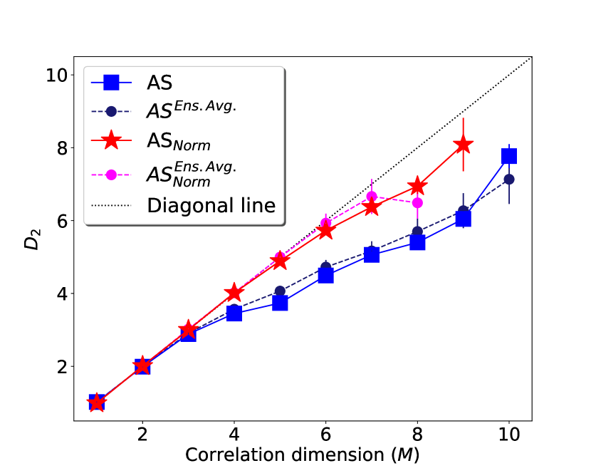
Figure 2: Variation of correlation dimension ($D_{2}$) with the embedding dimension ($M$) for $AS$ (square points) and $AS_{\rm Norm}$ (asterisks). The dotted line along the diagonal of the figure indicates the $D2$ variation as expected from an ideal stochastic process. $AS^{Ens.Avg.}$ and $AS_{Norm}^{Ens.Avg.}$ (round points) shows the variation averaged over an ensemble of 1000 AS & $AS_{Norm}$ time series, respectively (see Section 5).

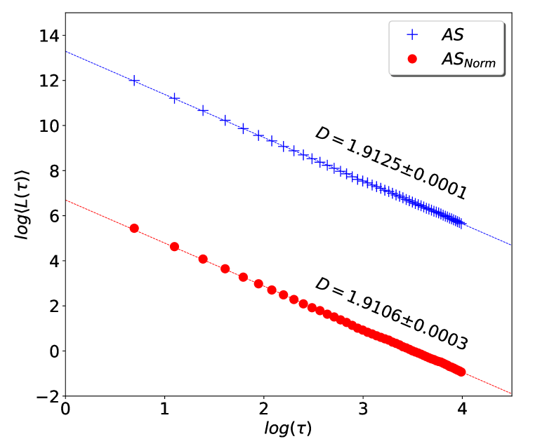
Figure 3: Variation of the length ($\langle{L(\tau)}\rangle$) with the time interval ($\tau$) for $AS$ and $AS_{Norm}$.

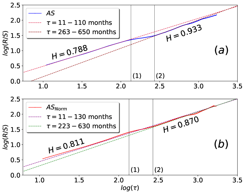
Figure 4: Variation of $R/S$ with time interval ($\tau$) for $AS$ (top) and $AS_{Norm}$ (bottom). $\tau=135$ months and $\tau=271$ months are indicated as (1) and (2).

A white noise process or a random walk process is defined by a Hurst exponent of $H=0.5$. When the time series has $H>0.5$, it is said to be persistent. Persistence is defined as the tendency for the process to have a memory of the previous step. That is, if there was an increase in the value of the time series, the following step would be more likely to have an increase as well. In such a case, the time series would cover more “distance” than a random walk would. Whereas, if $0<H<0.5$, then the time series is said to be anti-persistent. That is, an increase in the value of the time series is more likely to be followed by a decrease, and vice-versa. And in opposition to a persistent case, the time series would cover less “distance” than a random walk.

There are other methods to determine the Hurst exponent, and the value that is obtained is sensitive to the method used (Weron, 2002). In order to provide a confidence in the estimate of the Hurst exponent, and to ensure that the result is not method dependent, we shall compute Hurst exponent in two more methods, namely, Detrended Fluctuation Analysis and Periodogram Regression. As these methods are well described in the literature, we shall describe them briefly in Appendix A.

4 Results

The variation of $D_{2}$ as function of $M$ for the sunspot area asymmetry is shown in Figure 2. We find that the asymmetry and normalized asymmetry do not show the same behaviour. Nevertheless, in both cases, $D_{2}$ increases with an increase of $M$. The lack of saturation in $D_{2}$ implies that the sunspot area asymmetry is not governed by low-dimensional chaos, rather it might be driven by a high-dimensional or stochastic process. This conclusion is in general agreement with Carbonell et al. (1993) who also did not find the evidence of low-dimensional chaos in the asymmetry of sunspot area data during 1874–1989.

To confirm that the solar cycle asymmetry is really governed by stochastic or high-dimensional chaos, we observe the value of Higuchi’s dimension ($D$). As seen from Figure 3, for $AS$, $D=1.9125\pm 0.0001$, and for $AS_{Norm}$, $D=1.9106\pm 0.0003$. We know that when the value of $D$ for a curve is close to $2$, the curve behaves nearly like a surface, i.e., the curve is close to a space-filling curve. Hence, the self-similar nature for time series, i.e., the hallmark of low-dimensional chaos is absent. Therefore, we conclude that the process that generates the hemispheric asymmetry of sunspot area is very likely to be the result of an irregular or stochastic process.

Finally, we explore the memory of these irregular asymmetry data by computing the Hurst exponent ($H$). In Figure 4, we show the log-log plots for $R/S$ against $\tau$. The slope of this curve gives the H value. We, however, see two distinguishable linear scaling regimes, and hence one value of H for all $\tau$ is not adequately representing the data. The previous study for sunspot number cycle also indicted two distinct regimes (Suyal et al., 2009).

For $AS$, in the range: $\tau=11$–110 months, we find $H=0.79$, while for $\tau=263$–650 months, we obtain $H=0.94$ (Table 2). In between these two regimes, there is a small region during 135–271 months (marked by vertical lines in (Figure 4a)) with a weaker slope, which is possibly linked to a period of lower persistence in the trend. For $AS_{Norm}$ (Figure 4b), in the range $\tau=11$–130 months, we find $H=0.81$, while in the range: $\tau=233$–630 months, we get $H=0.87$. In this case, the change in the slope happens very slowly.

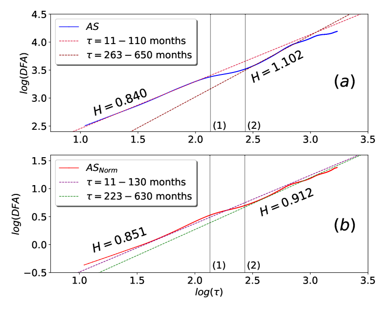
Figure 5: Variation of $DFA$ with time interval ($\tau$) for $AS$ (top) and $AS_{Norm}$ (bottom). $\tau=135$ and $\tau=271$ months are indicated as (1) and (2).

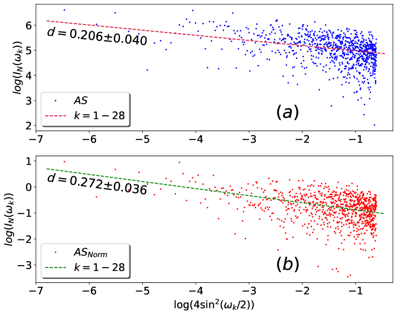
Figure 6: Periodogram Geweke-Porter-Hudak (GPH) Method for $AS$ (top) and $AS_{Norm}$ (bottom).

In the Detrended Fluctuation Analysis (DFA), we get similar results but the values of $H$ are slightly larger (Figure 5). For $AS$, in the range: $\tau=1$–110 months, we find $H=0.84$, while for $\tau=263-650$ months, we obtain $H=1.10$. Now, as discussed in Bryce & Sprague (2012); Ceballos & Largo (2017), we can point out that a value of $H$ above 1 is not impossible. It is a consequence of non-stationarity or a trend not being fully removed from the data. The reliability of DFA as a valid method has been questioned on similar grounds before. But since our R/S analysis still backs up the general result that the latter regime has a higher slope, we can safely negate the effect that this inconsistency may cause. (Table 2).

For $AS_{Norm}$, in the range: $\tau=11-130$ months, we find $H=0.85$, while in the range: $\tau=223-630$ months, we get $H=0.91$.

Using the Method of Periodogram Regression (Figure 6), for $AS$, we obtain $H(=0.5+0.21)=0.71$, while for $AS_{Norm}$, we obtain $H(=0.5+0.27)=0.77$. Unlike the case in $R/S$ Method and Detrended Fluctuation Analysis, the periodogram (Figure 6) does not show two distinct linear scaling regimes. However, the Hurst exponent being larger than 0.5, we can safely conclude that $AS$ and $AS_{Norm}$ time series are persistent in nature and the degree of persistence increases with the time-scale. Larger value of $H$ for $\tau\gtrapprox$ 22 years ($=264$ months), suggest that the memory of solar cycle asymmetry persists at least for two cycles.

We have obtained $H$ and $D$ graphically, using the Least Squares method for all of our plots; see e.g., Figure 3. We have also applied Bayesian linear regression to all our power law fits (Wheatland, 2004) using the justification towards a Bayesian method of fitting as opposed to a frequentist method, as explained in D’Huys et al. (2016). We use the Python module, PyMC3 (Salvatier et al., 2016) for this. We find that the differences in results lie in the range of $10^{-4}$ – $10^{-3}$, except in the case of of the periodogram method. In that case, for $AS$ and $AS_{Norm}$ we obtain the value of the Hurst exponents as $0.707\pm 0.179$ and $0.761\pm 0.132$, respectively using Bayesian linear regression, while these values obtained from previous Least Squares method are $0.706$ and $0.772$, respectively.

We recall that while computing $AS_{\rm Norm}$ using Equation (2), we took $AS_{\rm Norm}=0$ when both $A_{N}$ and $A_{S}$ are zero. Instead of this, if we replace these points by interpolating the neighbouring points, then this so-called zero-replacement strategy affects our computed results only marginally. (For example, from this zero-replacement $AS_{\rm Norm}$ data, the computed value of $D$ is 1.9077 and the values of $H$ are 0.8110 & 0.8693 (R/S method), 0.8469 & 0.9074 (DFA), and 0.7718 (PR). Compare these values with the corresponding values in Table 2.)

Table 2: Summary of results obtained for Higuchi’s dimension and Hurst exponents. In the forth and sixth columns, the values are the means and the standard deviations (errors) of the results obtained from an ensemble of 1000 AS & AS_Norm time series, respectively (see text).

Method	Window	Time Series
	(months)	AS	Ensemble of AS	ASNorm	Ensemble of ASNorm
Higuchi	2-55	1.912	1.915$\pm$0.002	1.911	1.916$\pm$0.002
Hurst (R$/$S)	11-110	0.788	0.783$\pm$0.008	0.811	0.813$\pm$0.007
	263-650	0.933	0.929$\pm$0.019	0.871	0.879$\pm$0.017
Hurst (DFA)	11-110	0.840	0.834$\pm$0.010	0.851	0.851$\pm$0.008
	263-650	1.102	1.096$\pm$0.022	0.912	0.920$\pm$0.018
Hurst (PR)	K = 28	0.706	0.704$\pm$0.039	0.772	0.775$\pm$0.028

5 Error Estimates

In our study, we used the monthly averaged hemispheric sunspot area as recorded in RGO. Unfortunately, in these data, no error information is given. Therefore we cannot make a direct estimate of error in our computed results. However, using the daily sunspot area data¹, we can make some estimate of the errors in the following way using a Bootstrapping technique (Efron & Tibshirani, 1993). Let us consider the daily sunspot area data of one month for both the northern and southern hemispheres. We produce 100 resampled datasets with the same size as the number of days for this month by randomly selecting daily pairs of values for north and south, and then computing the corresponding $AS$ and $AS_{Norm}$ for the resamples. We compute the mean for all of these resamples. And then, we compute the mean ($\mu$) and the standard deviation ($\sigma$) of the means of all the resampled datasets for a month. It can be easily seen that this mean is not necessarily the same as what we have used in our earlier analyses. With these $\mu$ and $\sigma$, we produce an ensemble of 1000 data points (deviate) from a Gaussian distribution and repeat this for all the months to get 1000 time series. Finally, perform our all the nonlinear time series analyses with this ensemble.

Black and magenta filled circles connecting dashed lines in Figure 2 show the average $D_{2}$ behaviour of the ensemble of 1000 $AS$ and $AS_{Norm}$ time series. The error bar represents the $\sigma$ of the computed $D_{2}$ of 1000 time series. In Table 2, forth and sixth columns show the mean and error (standard deviation) of $D$ and $H$ from the ensembles.

We clearly see that the mean values of the computed quantities ($D_{2}$, $D$, and $H$) of the ensemble of 1000 $AS$ & $AS_{Norm}$ time series are not too far from the ones computed from the original monthly mean time series. The values of $\sigma$ of the ensemble are also reasonably low, with the quantities being less than 1 standard deviation away from the computed values in most cases.

6 Discussion and Conclusion

We have explored some nonlinear properties of the underlying process behind the solar cycle asymmetry using nonlinear time series analysis. For this, we have used the hemispheric monthly sunspot area and number time series, which are the best proxies of the Sun’s large-scale magnetic flux available for a longer duration.

Following the literature, solar cycle asymmetry has been measured in two ways, namely, the hemispheric difference $AS$ and the normalized hemispheric asymmetry $AS_{Norm}$. We have used three methods of time series analyses to characterise the data.

From the analysis of the correlation dimension $D_{2}$, we find that the value of $D_{2}$ does not saturate for higher values of $M$. This indicates that there is no underlying presence of a low-dimensional chaotic attractor that could govern the asymmetry of sunspot area data, in agreement with the conclusion obtained in Carbonell et al. (1993). In other words, we can expect that the asymmetry is likely to be produced by irregular process.

In our fractal analysis, we see that the value obtained for the Higuchi’s fractal dimension ($D$) is close to $2$, which implies that a stochastic process or possibly a high-dimensional chaotic process is the cause of the asymmetry.

In all three methods of computation of Hurst exponent, we find the value of Hurst exponent $H$ is above 0.7 for $AS$ data and a little larger for $AS_{\rm Norm}$. We find multiple values of $H$ for the same time series. Its value decreases slightly after about 11 years (one cycle period) and then increases for windows larger than about 22 years. This change in the value of H and thus the persistence is more prominent in $AS$. In general, a memory can be observed for the asymmetry time series and it is larger in long-time scale (beyond 22 years; two cycles). From our analysis, we conclude that the monthly hemispheric asymmetry of sunspot area is dictated by a stochastic process with some amount of long-memory.

The results from hemispheric sunspot number, which is recently made available by Veronig et al. (2021) during 1874–2020, also shows similar behaviour (during the period May 1874 - September 2016) as that found in the hemispheric area data; §B.

Stochastic nature of hemispheric asymmetry supports the previous theoretical studies (e.g., Goel & Choudhuri, 2009; Olemskoy & Kitchatinov, 2013; Karak & Miesch, 2017; Schüssler & Cameron, 2018; Hazra & Nandy, 2019; Nepomnyashchikh et al., 2019) which explains the solar cycle asymmetry to be caused by the irregularity involved in the helical convective flow, and in particular the randomness involved in the Babcock–Leighton process (e.g., in the form of tilt of BMRs, emergence rate, meridional flow). Further, the presence of some long-term memory in asymmetry time series supports the existence of a finite memory of the sun’s magnetic field, which is possibly determined by the turbulent diffusion and pumping (Chatterjee & Choudhuri, 2006; Karak & Nandy, 2012; Karak & Miesch, 2017; Kitchatinov & Khlystova, 2021).

DATA AVAILABILITY

Sunspot area data used in the present study is obtained from the Royal Greenwich Observatory; http://solarscience.msfc.nasa.gov/greenwch.shtml. Data of our analyses presented in the article will be shared upon reasonable request to the corresponding author.

Appendix A Hurst exponent using different methods

In this section, we will determine the Hurst exponent by two other methods, namely, Detrended Fluctuation Analysis and Periodogram Regression.

The method of Detrended Fluctuation Analysis proposed by Peng et al. (1994) and also discussed in Weron (2002) can be summarized as follows. We choose a temporal window $\tau$, where $\tau_{0}\leq\tau\leq N$. Here, $\tau_{0}$ plays a similar role as the Theiler window plays in the $R/S$ method. For this $\tau$, we can divide the time series $X(t)$ into $d(=N-\tau+1)$ subseries

$$x_{i}(\tau):X(i),X(i+1),...,X(i+\tau-1)$$ (17)

for $i=1,2,3,...,d$. Note that each subseries $x_{i}(\tau)$ is of length $\tau$. Now, for each subseries $x_{i}(\tau)$, we create a cumulative time series

$$Y_{i}(\tau):X(i),\sum_{j=0}^{1}X(i+j),...,\sum_{j=0}^{\tau-1}X(i+j).$$ (18)

Now, we fit a least-squares line $\overline{Y}_{i}(\tau,x)=a_{i}x+b_{i}$ where, $x=1,2,...,\tau$, to $\{Y_{i}(\tau)\}$. Let, $S_{i}(\tau)$ be the root mean square fluctuation (i.e. standard deviation) of the Integrated and Detrended time series, given by

$$S_{i}(\tau)=\sqrt{\frac{1}{\tau}\sum_{x=1}^{\tau}(Y_{i,x}(\tau)-a_{i}x-b_{i})^{2}}$$ (19)

where, $Y_{i,x}(\tau)$ represents the x-th element of the cumulative time series $Y_{i}(\tau)$. Finally, we calculate the mean value of the root mean square fluctuation for all subseries of length $\tau$, $(DFA)_{\tau}$, given by

$$(DFA)_{\tau}=\frac{1}{d}\sum_{i=1}^{d}S_{i}(\tau)$$ (20)

Similar to the case of the $R/S$ analysis, a linear relationship on a double logarithmic paper of $(DFA)_{\tau}$ against $\tau$ indicates the presence of a power-law scaling

$$(DFA)_{\tau}=k\tau^{H}$$ (21)

where, $k$ is the proportionality constant and $H$ is the Hurst exponent. To obtain the values of the Hurst exponent, $(DFA)$ values are plotted for $\tau=11$–$1709$ months for both $AS$ and $AS_{Norm}$.

Now, we will discuss the method of Periodogram Regression proposed by Geweke & Porter-Hudak (1983). It is calcualted from the slope of the spectral density function of a fractionally integrated series at low frequencies.

For the time series, we start out by calculating the periodogram, which is a sample analogue of the spectral density. Given the time series $X(i)$ of length $N$, the periodogram is obtained as

$$I_{N}(\omega_{k})=\frac{1}{N}\left\lvert\sum_{t=1}^{N}X(t)e^{-i2\pi(t-1)\omega_{k}}\right\rvert^{2}$$ (22)

where, $\omega_{k}=k/N,k=1,2,...,[N/2]$ and $[X]$ denotes the greatest integer less than or equal to $X$ Note that, $I_{L}$ is the squared absolute value of the Fourier transform. The next step is to run a linear regression

$$\log\{I_{N}(\omega_{k})\}=a-\hat{d}\log\{4\sin^{2}(\omega_{k}/2)\}+\epsilon_{k}$$ (23)

at low Fourier frequencies $\omega_{k},k=1,2,...,K\leq[L/2]$. $\omega_{k},k=1,2,...,K\leq[N/2]$. The least squares estimate of the slope yields the differencing parameter $d=\hat{d}$ and $H=\hat{d}+0.5$. Next is how to set the value of $K$. Since, the differencing parameter $d$ is sensitive to the choice of $K$, we decided to keep it smaller than the standard value of $N^{0.5}$. We use $K=[N^{0.45}]=28$ in our analysis to determine the Hurst exponent, keeping in mind smaller powers of $N$ introduce large estimation errors. Once the differencing parameter $d$ was obtained, the Hurst exponent was obtained as $H=d+0.5$.

Appendix B Results from Hemispheric Sunspot Numbers

The sunspot number is probably the longest data available to study solar activity. However, the hemispheric data of sunspot number were available only from 1992. Recently, hemispheric sunspot number data has been derived and made publicly available (Veronig et al., 2021) during 1874–2020. As the sunspot number has been extensively used to study solar activity and it has a strong correlation with the sunspot area number, we present the results of our time-series analyses for the $AS$ and $AS_{Norm}$ computed from the sunspot number during the period May 1874 - September 2016. The results are presented in Table 3 and Figure 7.

Table 3: Summary of results obtained for Higuchi’s dimension and Hurst exponents from hemispheric sunspot numbers.

Method	Window	Time Series
	(months)	AS	ASNorm
Higuchi	2-55	1.90	1.90
Hurst (R$/$S)	11-110	0.83	0.83
	263-650	0.93	0.83
Hurst (DFA)	11-110	0.90	0.89
	263-650	1.07	0.88
Hurst (PR)	K = 28	0.73	0.76

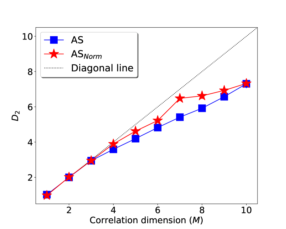
Figure 7: Variation of correlation dimension ($D_{2}$) with the embedding dimension ($M$) for $AS$ (square points) and $AS_{\rm Norm}$ (asterisks) calculated from hemispheric sunspot numbers.

References

- Arlt et al. (2016) Arlt R., Senthamizh Pavai V., Schmiel C., Spada F., 2016, A&A, 595, A104
- Ballester, J. L. et al. (2005) Ballester, J. L. Oliver, R. Carbonell, M. 2005, A&A, 431, L5
- Bell (1961) Bell B., 1961, Smithsonian Contributions to Astrophysics, 5, 69
- Bell (1962) Bell B., 1962, Smithsonian Contributions to Astrophysics, 5, 187
- Bryce & Sprague (2012) Bryce R. M., Sprague K. B., 2012, Scientific Reports, 2, 315
- Carbonell et al. (1993) Carbonell M., Oliver R., Ballester J. L., 1993, A&A, 274, 497
- Carbonell et al. (1994) Carbonell M., Oliver R., Ballester J. L., 1994, A&A, 290, 983
- Ceballos & Largo (2017) Ceballos R. F., Largo F. F., 2017, Imperial Journal of Interdisciplinary Research 2017), 3, 424
- Chang (2007) Chang H.-Y., 2007, Journal of Astronomy and Space Sciences, 24, 261–268
- Charbonneau (2020) Charbonneau P., 2020, Living Reviews in Solar Physics, 17, 4
- Chatterjee & Choudhuri (2006) Chatterjee P., Choudhuri A. R., 2006, Sol. Phys., 239, 29
- Choudhuri et al. (2007) Choudhuri A. R., Chatterjee P., Jiang J., 2007, Physical Review Letters, 98, 131103
- Chowdhury et al. (2013) Chowdhury P., Choudhary D. P., Gosain S., 2013, ApJ, 768, 188
- Duchlev (2001) Duchlev P. I., 2001, Solar Physics, 199, 211–215
- D’Huys et al. (2016) D’Huys E., Berghmans D., Seaton D. B., Poedts S., 2016, Solar Physics, 291, 1561–1576
- Efron & Tibshirani (1993) Efron B., Tibshirani R., 1993, An Introduction to the Bootstrap. Springer Science+Business Media, B. V.
- Geweke & Porter-Hudak (1983) Geweke J., Porter-Hudak S., 1983, J. Time Ser. Anal., 4, 221
- Goel & Choudhuri (2009) Goel A., Choudhuri A. R., 2009, Research in Astronomy and Astrophysics, 9, 115
- Grassberger & Procaccia (1983a) Grassberger P., Procaccia I., 1983a, Physica D Nonlinear Phenomena, 9, 189
- Grassberger & Procaccia (1983b) Grassberger P., Procaccia I., 1983b, Phys. Rev. Lett., 50, 346
- Hathaway (2015) Hathaway D. H., 2015, Living Reviews in Solar Physics, 12, 4
- Hazra (2021) Hazra G., 2021, Journal of Astrophysics and Astronomy, 42, 22
- Hazra & Nandy (2019) Hazra S., Nandy D., 2019, MNRAS, 489, 4329
- Higuchi (1988) Higuchi T., 1988, Physica D Nonlinear Phenomena, 31, 277
- Jevtić et al. (2001) Jevtić N., Schweitzer J. S., Cellucci C. J., 2001, A&A, 379, 611
- Jha et al. (2020) Jha B. K., Karak B. B., Mandal S., Banerjee D., 2020, ApJ, 889, L19
- Karak (2010) Karak B. B., 2010, ApJ, 724, 1021
- Karak (2020) Karak B. B., 2020, arXiv e-prints, p. arXiv:2009.06969
- Karak & Miesch (2017) Karak B. B., Miesch M., 2017, ApJ, 847, 69
- Karak & Miesch (2018) Karak B. B., Miesch M., 2018, ApJ, 860, L26
- Karak & Nandy (2012) Karak B. B., Nandy D., 2012, ApJ, 761, L13
- Karak et al. (2010) Karak B. B., Dutta J., Mukhopadhyay B., 2010, ApJ, 708, 862
- Karak et al. (2014) Karak B. B., Jiang J., Miesch M. S., Charbonneau P., Choudhuri A. R., 2014, Space Sci. Rev., 186, 561
- Karak et al. (2018) Karak B. B., Mandal S., Banerjee D., 2018, ApJ, 866, 17
- Kitchatinov & Khlystova (2021) Kitchatinov L. L., Khlystova A. A., 2021, ApJ
- Lemerle & Charbonneau (2017) Lemerle A., Charbonneau P., 2017, ApJ, 834, 133
- Letellier et al. (2006) Letellier C., Aguirre L. A., Maquet J., Gilmore R., 2006, A&A, 449, 379
- Li et al. (2009) Li K. J., Chen H. D., Zhan L. S., Li Q. X., Gao P. X., Mu J., Shi X. J., Zhu W. W., 2009, Journal of Geophysical Research (Space Physics), 114, A04101
- Mandal et al. (2017) Mandal S., Karak B. B., Banerjee D., 2017, ApJ, 851, 70
- Mandelbrot & Wallis (1969) Mandelbrot B. B., Wallis J. R., 1969, Water Resources Research, 5, 321
- McIntosh et al. (2013) McIntosh S. W., et al., 2013, ApJ, 765, 146
- Misra et al. (2006) Misra R., Harikrishnan K. P., Ambika G., Kembhavi A. K., 2006, The Astrophysical Journal, 643, 1114
- Mordvinov & Kitchatinov (2004) Mordvinov A. V., Kitchatinov L. L., 2004, Astronomy Reports, 48, 254
- Mordvinov & Kitchatinov (2019) Mordvinov A. V., Kitchatinov L. L., 2019, Sol. Phys., 294, 21
- Mordvinov et al. (2020) Mordvinov A. V., Karak B. B., Banerjee D., Chatterjee S., Golubeva E. M., Khlystova A. I., 2020, arXiv e-prints, p. arXiv:2009.11174
- Nepomnyashchikh et al. (2019) Nepomnyashchikh A., Mandal S., Banerjee D., Kitchatinov L., 2019, A&A, 625, A37
- Norton et al. (2014) Norton A. A., Charbonneau P., Passos D., 2014, Space Sci. Rev., 186, 251
- Olemskoy & Kitchatinov (2013) Olemskoy S. V., Kitchatinov L. L., 2013, ApJ, 777, 71
- Oliver & Ballester (1996) Oliver R., Ballester J. L., 1996, Solar Physics, 169, 215–224
- Ostriakov & Usoskin (1990a) Ostriakov V. M., Usoskin I. G., 1990a, Sol. Phys., 127, 405
- Ostriakov & Usoskin (1990b) Ostriakov V. M., Usoskin I. G., 1990b, Sol. Phys., 127, 405
- Packard et al. (1980) Packard N. H., Crutchfield J. P., Farmer J. D., Shaw R. S., 1980, Phys. Rev. Lett., 45, 712
- Parker (1955) Parker E. N., 1955, ApJ, 122, 293
- Peng et al. (1994) Peng C. K., Buldyrev S. V., Havlin S., Simons M., Stanley H. E., Goldberger A. L., 1994, Phys. Rev. E, 49, 1685
- Priyal et al. (2014) Priyal M., Banerjee D., Karak B. B., Muñoz-Jaramillo A., Ravindra B., Choudhuri A. R., Singh J., 2014, ApJ, 793, L4
- Ruzmaikin et al. (1994) Ruzmaikin A., Feynman J., Robinson P., 1994, Sol. Phys., 149, 395
- Salvatier et al. (2016) Salvatier J., Wiecki T. V., Fonnesbeck C., 2016, PeerJ Computer Science, 2, e55
- Schreiber (1999) Schreiber T., 1999, Phys. Rep., 308, 1
- Schüssler & Cameron (2018) Schüssler M., Cameron R. H., 2018, A&A, 618, A89
- Sokoloff & Nesme-Ribes (1994) Sokoloff D., Nesme-Ribes E., 1994, A&A, 288, 293
- Stenflo & Kosovichev (2012) Stenflo J. O., Kosovichev A. G., 2012, ApJ, 745, 129
- Suyal et al. (2009) Suyal V., Prasad A., Singh H. P., 2009, Sol. Phys., 260, 441
- Swinson et al. (1986) Swinson D. B., Koyama H., Saito T., 1986, Sol. Phys., 106, 35
- Takens (1981) Takens F., 1981, Detecting strange attractors in turbulence. p. 366, doi:10.1007/BFb0091924
- Theiler (1986) Theiler J., 1986, Phys. Rev. A, 34, 2427
- Verma (1987) Verma V. K., 1987, Sol. Phys., 114, 185
- Veronig et al. (2021) Veronig A. M., Jain S., Podladchikova T., Pötzi W., Clette F., 2021, A&A, 652, A56
- Wang et al. (2015) Wang Y.-M., Colaninno R. C., Baranyi T., Li J., 2015, ApJ, 798, 50
- Watari (1996) Watari S., 1996, Sol. Phys., 163, 259
- Weron (2002) Weron R., 2002, Physica A Statistical Mechanics and its Applications, 312, 285
- Wheatland (2004) Wheatland M. S., 2004, ApJ, 609, 1134
- Yi (1992) Yi W., 1992, Journal of the Royal Astronomical Society of Canada, 86, 89–98