Simulating High-Dimensional Multivariate Data using the Bigsimr R Package

Abstract

It is critical to accurately simulate data when employing Monte Carlo techniques and evaluating statistical methodology. Measurements are often correlated and high dimensional in this era of big data, such as data obtained in high-throughput biomedical experiments. Due to the computational complexity and a lack of user-friendly software available to simulate these massive multivariate constructions, researchers resort to simulation designs that posit independence or perform arbitrary data transformations. To close this gap, we developed the Bigsimr Julia package with R and Python interfaces. This paper focuses on the R interface. These packages empower high-dimensional random vector simulation with arbitrary marginal distributions and dependency via a Pearson, Spearman, or Kendall correlation matrix. bigsimr contains high-performance features, including multi-core and graphical-processing-unit-accelerated algorithms to estimate correlation and compute the nearest correlation matrix. Monte Carlo studies quantify the accuracy and scalability of our approach, up to $d=10,000$. We describe example workflows and apply to a high-dimensional data set — RNA-sequencing data obtained from breast cancer tumor samples.

© A.G. Schissler. This is an Open Access article distributed under the terms of the Creative Commons License Attribution-NonCommercial-ShareAlike 4.0 International (CC BY-NC-SA 4.0) (https://creativecommons.org/licenses/by-nc-sa/4.0/), which permits reusers to distribute, remix, adapt, and build upon the material in any medium or format for noncommercial purposes only, and only so long as attribution is given to the creator. If you remix, adapt, or build upon the material, you must license the modified material under identical terms.

Keywords high-dimensional data  $\cdot$ multivariate simulation  $\cdot$ nonparametric correlation  $\cdot$ Gaussian copula  $\cdot$ RNA-sequencing data  $\cdot$ breast cancer

1 Introduction

Massive high-dimensional (HD) data sets are now common in many areas of scientific inquiry. As new methods are developed for data analysis, a fundamental challenge lies in designing and conducting simulation studies to assess the operating characteristics of proposed methodology — such as false positive rates, statistical power, interval coverage, and robustness. Further, efficient simulation empowers statistical computing strategies, such as the parametric bootstrap (Chernick 2008) to simulate from a hypothesized null model, providing inference in analytically challenging settings. Such Monte Carlo (MC) techniques become difficult for HD dependent data using existing algorithms and tools. This is particularly true when simulating massive multivariate, non-normal distributions, arising in many fields of study.

As others have noted, it can be vexing to simulate dependent, non-normal/discrete data, even for low-dimensional (LD) settings (Madsen and Birkes 2013; Xiao and Zhou 2019). For continuous non-normal LD multivariate data, the well-known NORmal To Anything (NORTA) algorithm (Cario and Nelson 1997) and other copula approaches (Nelsen 2007) are well-studied and implemented in publicly-available software (Yan 2007; Chen 2001). Yet these approaches do not scale in a timely fashion to HD problems (X. Li et al. 2019). For discrete data, early simulation strategies had major flaws, such as failing to obtain the full range of possible correlations — such as admitting only positive correlations (Park, Park, and Shin 1996). While more recent approaches (Madsen and Birkes 2013; Xiao 2017; Barbiero and Ferrari 2017) have remedied this issue for LD problems, the existing tools are not designed to scale to high dimensions.

Another central issue lies in characterizing dependence between components in the HD random vector. The choice of correlation in practice usually relates to the eventual analytic goal and distributional assumptions of the data (e.g., non-normal, discrete, infinite support, etc.). For normal data, the Pearson product-moment correlation describes the dependence perfectly. However, simulating arbitrary random vectors that match a target Pearson correlation matrix is computationally intense (Chen 2001; Xiao 2017). On the other hand, an analyst might consider use of nonparametric correlation measures to better characterize monotone, non-linear dependence, such as Spearman’s $\rho$ and Kendall’s $\tau$. Throughout, we focus on matching these nonparametric dependence measures, as our aim lies in modeling non-normal data and these rank-based measures possess invariance properties enabling our proposed methodology. We do, however, implement Pearson matching, but several layers of approximation are required.

With all this in mind, we present a scalable, flexible multivariate simulation algorithm. The crux of the method lies in the construction of a Gaussian copula in the spirit of the NORTA procedure. As we will describe in more detail, the algorithm’s design leverages useful properties of nonparametric correlation measures, namely invariance under monotone transformation and well-known closed-form relationships between dependence measures for the multivariate normal (MVN) distribution. For our method, we developed a high-performance implementation: the Bigsimr Julia package, with R and Python interfaces bigsimr.

This article proceeds by providing background information, including a description of a motivating example application: RNA-sequencing (RNA-seq) breast cancer data. Then we describe and justify our simulation methodology and related algorithms. We proceed by providing an illustrative LD bigsimr workflow. Next we conduct MC studies under various bivariate distributional assumptions to evaluate performance and accuracy. After the MC evaluations, we simulate random vectors motivated by our RNA-seq example, evaluate the accuracy, and provide example statistical computing tasks, namely MC estimation of joint probabilities and evaluating HD correlation estimation efficiency. Finally, we discuss the method’s utility, limitations, and future directions.

2 Background

The Bigsimr package presented here provides multiple high-performance algorithms that operate with HD multivariate data. All these algorithms were originally designed to support a single task: to generate random vectors drawn from multivariate probability distributions with given marginal distributions and dependency metrics. Specifically, our goal is to efficiently simulate a large number, $B$, of HD random vectors ${\bf Y}=(Y_{1},\ldots,Y_{d})^{\top}$ with correlated components and heterogeneous marginal distributions, described via cumulative distribution functions (CDFs) $F_{i},i=1,\ldots,d$.

When designing this methodology, we developed the following properties to guide our effort. We divide the properties into two categories: (1) basic properties (BP) and ‘scalability’ properties (SP). The BPs are adapted from an existing criteria due to Nikoloulopoulos (2013). A suitable simulation strategy should possess the following properties:

• BP1: A wide range of dependences, allowing both positive and negative values, and, ideally, admitting the full range of possible values.

• BP2: Flexible dependence, meaning that the number of dependence parameters can be equal to the number of bivariate pairs in the vector.

• BP3: Flexible marginal modeling, generating heterogeneous data — including mixed continuous and discrete marginal distributions.

Moreover, the simulation method must scale to high dimensions:

• SP1: Procedure must scale to high dimensions with practical computation times.

• SP2: Procedure must scale to high dimensions while maintaining accuracy.

2.1 Motivating example: RNA-seq data

Simulating HD, non-normal, correlated data motivates this work, in pursuit of modeling RNA-sequencing (RNA-seq) data (Wang, Gerstein, and Snyder 2009; Conesa et al. 2016) derived from breast cancer patients. The RNA-seq data-generating process involves counting how often a particular form of messenger RNA (mRNA) is expressed in a biological sample. RNA-seq platforms typically quantify the entire transcriptome in one experimental run, resulting in HD data. For human-derived samples, this results in count data corresponding to over 20,000 genes (protein-coding genomic regions) or even over 77,000 isoforms when alternatively-spliced mRNA are counted (Schissler et al. 2019). Importantly, due to inherent biological processes, gene expression data exhibit correlation (co-expression) across genes (Efron 2007; Schissler, Piegorsch, and Lussier 2018).

We illustrate our methodology using the Breast Invasive Carcinoma (BRCA) data set housed in The Cancer Genome Atlas (TCGA; see Acknowledgments). For ease of modeling and simplicity of exposition, we only consider high expressing genes. In turn, we begin by filtering to retain the top r d of the highest-expressing genes (in terms of median expression) of the over 20,000 gene measurements from $N=rnrow(example_{b}rca)$ patients’ tumor samples. This gives a great number of pairwise dependencies among the marginals (specifically, $rchoose(d,2)$ correlation parameters). Table 1 displays RNA-seq counts for three selected high-expressing genes for the first five patients’ breast tumor samples. To help visualize the bivariate relationships for these three selected genes across all patients, Figure 1 displays the marginal distributions and estimated Spearman’s correlations.

Table 1: mRNA expression for three selected high-expressing genes, STAU1, FKBP1A, NME2, for the first five patients in the TCGA BRCA data set.

Patient ID	STAU1	FKBP1A	NME2
TCGA-A1-A0SB	10440	11354	17655
TCGA-A1-A0SD	21523	20221	14653
TCGA-A1-A0SE	21733	22937	35251
TCGA-A1-A0SF	11866	19650	16551
TCGA-A1-A0SG	12486	12089	10434

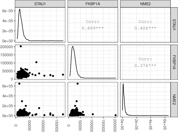
Figure 1: Pairwise scatterplots for three example genes (Table 1), with estimated Spearman’s correlations and marginal density estimates displayed. The data possess outliers, heavy-right tails, are discrete, and have non-trivial intergene correlations. Modeling these data motivate our simulation methodology.

2.2 Measures of dependency

In multivariate analysis, an analyst must select a metric to quantify dependency. The most widely-known is the Pearson correlation coefficient that describes the linear association between two random variables $X$ and $Y$, and, it is given by

$$\rho_{P}(X,Y)=\frac{E(XY)-E(X)E(Y)}{\left[\mathrm{Var}(X)\mathrm{Var}(Y)\right]^{1/2}}.$$ (1)

As Madsen and Birkes (2013) and Mari and Kotz (2001) discuss, for a bivariate normal $(X,Y)$ random vector, the Pearson correlation completely describes the dependency between the components. For non-normal marginals with monotone correlation patterns, however, $\rho_{P}$ suffers some drawbacks and may mislead or fail to capture important relationships (Mari and Kotz 2001). Alternatively, analysts often prefer rank-based correlation measures to describe the degree of monotonic association.

Two nonparametric, rank-based measures common in practice are Spearman’s correlation (denoted $\rho_{S}$) and Kendall’s $\tau$. Spearman’s $\rho_{S}$ has an appealing correspondence as the Pearson correlation coefficient on ranks of the values, thereby capturing nonlinear yet monotone relationships. Kendall’s $\tau$, on the other hand, is the difference in probabilities of concordant and discordant pairs of observations, $(X_{i},Y_{i})$ and $(X_{j},Y_{j})$ (concordance meaning that orderings have the same direction, e.g., if $X_{i}<X_{j}$, then $Y_{i}<Y_{j}$). Note that concordance is determined by the ranks of the values, not the values themselves. Both $\tau$ and $\rho_{S}$ are invariant under monotone transformations of the underlying random variates. As we will describe more fully in the Algorithms section, this property enables matching rank-based correlations with speed (SP1) and accuracy (SP2).

Correspondence among Pearson, Spearman, and Kendall correlations

There is no closed form, general correspondence among the rank-based measures and the Pearson correlation coefficient, as the marginal distributions $F_{i}$ are intrinsic in their calculation. For bivariate normal vectors, however, the correspondence is well-known:

$$\rho_{P}=\sin\left(\tau\times\frac{\pi}{2}\right),$$ (2)

and similarly for Spearman’s $\rho$ (Kruskal 1958),

$$\rho_{P}=2\times\sin\left(\rho_{S}\times\frac{\pi}{6}\right).$$ (3)

Marginal-dependent bivariate correlation bounds

Given two marginal distributions, $\rho_{P}$ is not free to vary over the entire range of possible correlations $[-1,1]$. The Frechet-Hoeffding bounds are well-studied (Nelsen 2007; Barbiero and Ferrari 2017). These constraints cannot be overcome through algorithm design. In general, the bounds are given by

$$\rho_{P}^{max}=\rho_{P}\left(F^{-1}_{1}(U),F^{-1}_{2}(U)\right),\quad\rho_{P}^{min}=\rho_{P}\left(F^{-1}_{1}(U),F^{-1}_{2}(1-U)\right)$$ (4)

where $U$ is a uniform random variable on $(0,1)$ and $F^{-1}_{1},F^{-1}_{2}$ are the inverse CDFs of $X_{1}$ and $X_{2}$, respectively, defined as

$$F_{i}^{-1}=\inf\{y:F_{i}(y)\geq u\}$$ (5)

when the variables are discrete.

2.3 Gaussian copulas

There is a connection of our simulation strategy to Gaussian copulas (Nelsen 2007). A copula is a distribution function on $[0,1]^{d}$ that describes a multivariate probability distribution with standard uniform marginals. This provides a powerful, natural way to characterize joint probability. Consequently, the study of copulas is an important and active area of statistical theory and practice. For any random vector ${\bf X}=(X_{1},\ldots,X_{d})^{\top}$ with CDF $F$ and marginal CDFs $F_{i}$ there is a copula function $C(u_{1},\ldots,u_{d})$ satisfying

$$F(x_{1},\ldots,x_{d})={\mathbb{P}}(X_{1}\leq x_{1},\ldots,X_{d}\leq x_{d})=C(F_{1}(x_{1}),\ldots,F_{d}(x_{d})),\quad x_{i}\in{\mathbb{R}},i=1,\ldots,d.$$ (6)

A Gaussian copula has marginal CDFs that are all standard normal, $F_{i}=\Phi,\forall\,i$, . This representation corresponds to a multivariate normal (MVN) distribution with standard normal marginal distributions and covariance matrix $R_{P}$. Since the marginals are standardized to have unit variance, this $R_{P}$ is also Pearson correlation matrix. If $F_{R}$ is the CDF of such a multivariate normal distribution, then the corresponding Gaussian copula $C_{R}$ is defined through

$$F_{R}(x_{1},\ldots,x_{d})=C_{R}(\Phi(x_{1}),\ldots,\Phi(x_{d})),$$ (7)

where $\Phi(\cdot)$ is the standard normal CDF.

Here, the copula function $C_{R}$ is the CDF of the random vector $(\Phi(X_{1}),\ldots,\Phi(X_{d}))$, where $(X_{1},\ldots,X_{d})\sim N_{d}({\bf 0},R_{P})$.

Sklar’s Theorem (Úbeda-Flores and Fernández-Sánchez 2017) guarantees that given inverse CDFs $F_{i}^{-1}$s and a valid correlation matrix (within the Frechet bounds) a random vector can be obtained via transformations involving copula functions. For example, using Gaussian copulas, we can construct a random vector ${\bf Y}=(Y_{1},\ldots,Y_{d})^{\top}$ with $Y_{i}\sim F_{i}$, viz. $Y_{i}=F_{i}^{-1}(\Phi(X_{i})),i=1,\ldots,d$, where $(X_{1},\ldots,X_{d})\sim N_{d}({\bf 0},R_{P})$.

2.4 Other Multivariate Simulation Packages

To place Bigsimr’s implementation and algorithms in context of existing approaches, we qualitatively compare Bbigsimr to other multivariate simulation packages. In R, the MASS package’s mvnorm() has long been available to produce random vectors from multivariate normal (and $t$) distributions. This procedure cannot simulate from arbitrary margins and dependency measures and it fails to readily scale to high dimensions. SAS PROC SIMNORMAL and Python’s NumPy random.multivariate_normal both do similar tasks. Recently, the high-performance R package mvnfast (Fasiolo 2016) has been released, which provides HD multivariate normal generation. However, lacks flexibility in marginal models and dependency modeling. For dependent discrete data, LD R packages exist, such as GenOrd. For copula computation, the full-featured R package copula provides many different copulas and a fairly general LD random generator rCopula(). High-dimesional random vector generation via copula takes an impractical amount of computing time (X. Li et al. 2019). The nortaRA R package matches Pearson coefficients near exactly and is reasonable for LD settings. Finally, we know of no other R package that can produce HD random vectors with flexible margins and dependence structure. Table 2 summarizes the above discussion.

Table 2: Comparison of selected features of bigsimr to existing R packages for multivariate simulation.

Package	Scales to HD	Hetereogenous Margins	Flexible Dependence
MASS	No	No	No
mvnfast	Yes	No	No
GenOrd	No	Discrete margins	Yes
copula	No	Yes	No
nortaRA	No	Yes	No
bigsimr	Yes	Yes	Yes

3 Algorithms

This section describes our methods for simulating a random vector $\bf Y$ with $Y_{i}$ components for $i=1,\ldots,d$. Each $Y_{i}$ has a specified marginal CDF $F_{i}$ and its inverse $F^{-1}_{i}$. To characterize dependency, every pair $(Y_{i},Y_{j})$ has a given Pearson correlation $\rho_{P}$, Spearman correlation $\rho_{S}$, and/or Kendall’s $\tau$. The method can be described as a high-performance Gaussian copula (Equation 7) providing a HD NORTA-inspired algorithm.

3.1 NORmal To Anything (NORTA)

The well-known NORTA algorithm (Cario and Nelson 1997) simulates a random vector $\bf Y$ with variance-covariance matrix $\Sigma_{\bf Y}$. Specifically, NORTA algorithm proceeds as follows:

1. Simulate a random vector $\bf Z$ with $d$ independent and identically distributed (iid) standard normal components.

2. Determine the input matrix $\Sigma_{\bf Z}$ that corresponds with the specified output $\Sigma_{\bf Y}$.

3. Produce a Cholesky factor $M$ of $\Sigma_{\bf Z}$ such that $MM^{\prime}=\Sigma_{\bf Z}$.

4. Set $X$ by $X\leftarrow MZ$.

5. $\text{Return}\;{\bf Y}\;\text{where}\;Y_{i}\leftarrow F_{i}^{-1}[\Phi(X_{i})],\;i=1,...,d$.

With modern parallel computing, steps 1, 3, 4, 5 are readily implemented as high-performance, multi-core and/or graphical-processing-unit (GPU) accelerated algorithms — providing fast scalability to HD.

Matching specified Pearson correlation coefficients exactly (step 2 above), however, is computationally costly. In general, there is no convenient correspondence between the components of the input $\Sigma_{\bf Z}$ and target $\Sigma_{\bf Y}$. Matching the correlations involves evaluating or approximating $\binom{d}{2}$ integrals of the form

$$\mathrm{E}\left[Y_{i}Y_{j}\right]=\int_{-\infty}^{\infty}\int_{-\infty}^{\infty}F_{i}^{-1}\left[\Phi(z_{i})\right]F_{j}^{-1}\left[\Phi(z_{j})\right]\phi(z_{i},z_{j},\rho_{z})dz_{i}dz_{j},$$ (8)

where $\phi(\cdot)$ is the joint probability density function of two correlated standard normal variables. For HD simulation, exact evaluation may become too costly to enable practical simulation studies. Our remedy to enable HD Pearson matching in bigsimr is Hermite polynomial approximation of these $\binom{d}{2}$ double integrals, as suggested by Xiao and Zhou (2019).

NORTA in higher dimensions

Sklar’s theorem provides a useful characterization of multivariate distributions through copulas. In practice, however, the particulars of the simulation algorithm affect which joint distributions may be simulated. Even in LD spaces (e.g., $d=3$), there exist valid multivariate distributions with feasible Pearson correlation matrices that NORTA cannot match exactly (S. T. Li and Hammond 1975). This occurs when the bivariate transformations are applied to find the input correlation matrix, yet when combined, the resultant matrix becomes non-positive definite. These situations do occur, even using exact analytic calculations. Such problematic target correlation matrices are termed NORTA defective.

Ghosh and Henderson (2002) conducted a study to estimate the probability of encountering NORTA defective matrices while increasing the dimension $d$. They found that for what is now considered low-to-moderate dimensions ($d\approx 20$), almost all feasible matrices are NORTA defective. This stems from the concentration of measure near the boundary of the space of all possible correlation matrices as dimension increases. Unfortunately, it is precisely near this boundary that NORTA defective matrices reside.

There is hope, however, as Ghosh and Henderson (2002) also showed that replacing an non-positive definite input correlation matrix with a close proxy will give approximate matching to the target — with adequate performance for moderate $d$. This provides evidence that our nearest positive definite (PD) augmented approach has promise to provide adequate accuracy if our input matching scheme returns an indefinite Pearson correlation matrix.

3.2 Random vector generator

We now describe our algorithm to generate random vectors, which extends NORTA to HD via nearest correlation matrix replacement and provides rank-based dependency matching:

1. Mapping step, either

   • Convert the target Spearman correlation matrix $R_{S}$ to the corresponding MVN Pearson correlation $R_{X}$. Alternatively,

   • Convert the target Kendall $\tau$ matrix $R_{K}$ to the corresponding MVN Pearson correlation $R_{X}$. Alternatively,

   • Convert the target Pearson correlation matrix to $R_{P}$ to the corresponding, approximate MVN Pearson correlation $R_{X}$.

2. Check correlation matrix admissibility and, if not, compute the nearest correlation matrix.

   • Check that $R_{X}$ is a correlation matrix, a positive definite matrix with 1’s along the diagonal.

   • If the mapping produced an $R_{X}$ that is a correlation matrix, we describe the matrix as admissible in this scheme and retain $R_{X}$. Otherwise,

   • Replace $R_{X}$ with the nearest correlation matrix $\tilde{R}_{X}$, in the Frobenius norm and the result will be approximate.

3. Gaussian copula

   • Generate ${\bf X}=(X_{1},\ldots,X_{d})\sim N_{d}({\bf 0},R_{X})$.

   • Transform ${\bf X}$ to ${\bf U}=(U_{1},\ldots,U_{d})$ viz. $U_{i}=\Phi(X_{i})$, $i=1,\ldots,d$.

   • Return ${\bf Y}=(Y_{1},\ldots,Y_{d})$, where $Y_{i}=F_{i}^{-1}(U_{i})$, $i=1,\ldots,d$.

Step 1: Mapping step. We first employ the closed-form relationships between $\rho_{S}$ and $\tau$ with $\rho_{P}$ for bivariate normal random variables via Equations 2 and 3, respectively (implemented as cor_covert()). Initializing our algorithm to match the nonparametric correlations by computing these equations for all pairs is computationally trivial.

For the computationally expensive process to match Pearson correlations, we approximate Equation 8 for all pairs of margins. To this end, we implement the approximation scheme introduced by (Xiao and Zhou 2019). Briefly, the many double integrals of the form in 8 are approximated by weighted sums of Hermite polynomials. Matching coefficients for pairs of continuous distributions is made tractable by this method, but for discrete distributions (especially discrete distributions with large support sets or infinite support), the approximation is computationally expensive. To remedy this, we further approximate discrete distributions by a continuous distribution using Generalized S-Distributions (Muino, Voit, and Sorribas 2006).

Step 2: Admissibility check and nearest correlation matrix computation. Once $R_{X}$ has been determined, we check admissibility of the adjusted correlation via the steps described above. If $R_{X}$ is not a valid correlation matrix, then we compute the nearest correlation matrix. Finding the nearest correlation matrix is a common statistical computing problem. The defacto function in R is Matrix::nearPD, an alternating projection algorithm due to Higham (2002). As implemented, the function fails to scale to HD. Instead, we provide the quadratically-convergent algorithm based on the theory of strongly semi-smooth matrix functions (Qi and Sun 2006). The nearest correlation matrix problem can be written down as the following convex optimization problem: $\mathrm{min}\quad\frac{1}{2}\|R_{X}-X\|^{2},\quad\mathrm{s.t.}\quad X_{ii}=1,\quad i=1,\ldots,n,\quad X\in S_{+}^{n}$.

For nonparametric correlation measures, our algorithm allows the generation of HD multivariate data with arbitrary marginal distributions with a broad class of admissible Spearman correlation matrices and Kendall $\tau$ matrices. The admissible classes consist of the matrices that map to a Pearson correlation matrix for a MVN. In particular, if we let $X$ be MVN with $d$ components and denote $\Omega_{P}=\{R_{P}:R_{P}\textrm{ is a Pearson correlation matrix for }X\},\quad\Omega_{K}=\{R_{K}:R_{K}\textrm{ is a Kendall correlation matrix for }X\},\quad\Omega_{S}=\{R_{S}:R_{S}\textrm{ is a Spearman correlation matrix for }X\}$. There are 1-1 mappings between these sets. We conjecture that the sets of admissible $R_{S}$ and $R_{K}$ are not highly restrictive. In particular, $R_{P}$ is approximately $R_{S}$ for a MVN, suggesting that the admissible set $\Omega_{S}$ should be flexible as $R_{P}$ can be any PD matrix with 1’s along the diagonal. We provide methods to check whether a target $R_{S}$ is an element of the admissible set $\Omega_{S}$.

There is an increasing probability of encountering an inadmissible correlation matrix as dimension increases. In our experience, the mapping step for large $d$ almost always produces a $R_{X}$ that is not a correlation matrix. In Section LABEL:package, we provide a basic method of how to quantify and control the approximation error. Further, the RNA-seq example in Section 6 provides an illustration of this in practice.

Step 3: Gaussian copula. The final step implements a NORTA-inspired, Gaussian copula approach to produce the desired margins. Steps 1 and 2 determine the MVN Pearson correlation values that will eventually match the target correlation. Step 3 requires a fast MVN simulator, a standard normal CDF, and well-defined quantile functions for marginals. The MVN is transformed to a copula (distribution with standard uniform margins) by applying the normal CDF $\Phi(\cdot)$. Finally, the quantile functions $F_{i}^{-1}$ are applied across the margins to return the desired random vector ${\bf Y}$.

4 The bigsimr R package

This section describes a bivariate random vector simulation workflow via the bigsimr R package. This R package provides an interface to the native code written in Julia (registered as the Bigsimr Julia package). In addition to the native Julia Bigsimr package and R interface bigsimr, we also provide a Python interface bigsimr that interfaces with the Julia Bigsimr package. The Julia package provides a high-performance implementation of our proposed random vector generation algorithm and associated functions (see Section 3).

The subsections below describe the basic use of the bigsimr R package by stepping through an example workflow using the data set airquality that contains daily air quality measurements in New York, May to September 1973 (Chambers et al. 1983). This workflow proceeds from setting up the computing environment, to data wrangling, estimation, simulation configuration, random vector generation, and, finally, result visualization.

4.1 Bivariate example

We illustrate the use of bigsimr using the New York air quality data set (airquality) included in the R datasets package. First, we load the bigsimr library and a few other convenient data science packages, including the syntactically-elegant tidyverse suite of R packages. The code chunk below prepares the computing environment:

library("tidyverse")

library("bigsimr")

# Activate multithreading in Julia

Sys.setenv(JULIA_NUM_THREADS = parallel::detectCores())

# Load the Bigsimr and Distributions Julia packages

bs <- bigsimr_setup()

dist <- distributions_setup()

Here, we describe a minimal working example — a bivariate simulation of two airquality variables: Temperature, in degrees Fahrenheit, and Ozone level, in parts per billion.

df <- airquality %>% select(Temp, Ozone) %>% drop_na()

glimpse(df)

## Rows: 116
## Columns: 2
## $ Temp  <int> 67, 72, 74, 62, 66, 65, 59, 61, 74, 69, 66, 68, 58, 64, 66, 5...
## $ Ozone <int> 41, 36, 12, 18, 28, 23, 19, 8, 7, 16, 11, 14, 18, 14, 34, 6, ...

Figure 2 visualizes the bivariate relationship between Ozone and Temperature. We aim to simulate random two-component vectors mimicking this structure. The margins are not normally distributed; Ozone level exhibits a strong positive skew.

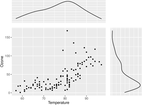
Figure 2: Bivariate scatterplot of Ozone versus Temp with estimated marginal densities. The Ozone data are modeled marginally as log-normal and the Temperature data as normal.

Next, we specify the marginal distributions and correlation coefficient (both type and magnitude). Here the analyst is free to be creative. For this example, we avoid goodness-of-fit considerations to determine the marginal distributions. It is sensible without domain knowledge to estimate these quantities from the data, and bigsimr contains fast functions designed for this task.

4.2 Specifying marginal distributions

Based on the estimated densities in Figure 2, we assume Temp is normally distributed and Ozone is log-normally distributed, as the latter values are positive and skewed. We use the classical unbiased estimators for the normal distribution’s parameters and maximum likelihood estimators for the log-normal parameters:

df %>% select(Temp) %>%

  summarise_all(.funs = c(mean = mean, sd = sd))

##       mean       sd
## 1 77.87069 9.485486

mle_mean <- function(x) mean(log(x))

mle_sd <- function(x) mean( sqrt( (log(x) - mean(log(x)))^2 ) )

df %>%

  select(Ozone) %>%

  summarise_all(.funs = c(meanlog = mle_mean, sdlog = mle_sd))

##    meanlog     sdlog
## 1 3.418515 0.6966689

Now, we configure the input marginals for later input into rvec. The marginal distributions are specified using Julia’s Distributions package and stored in a vector.

margins <- c(dist$Normal(mean(df$Temp), sd(df$Temp)),

             dist$LogNormal(mle_mean(df$Ozone), mle_sd(df$Ozone)))

4.3 Specifying correlation

The user must decide how to describe correlation based on the particulars of the problem. For non-normal data in our scheme, we advocate the use of Spearman’s $\rho$ correlation matrix $R_{S}$ or Kendall’s $\tau$ correlation matrix $R_{K}$. We also support Pearson correlation coefficient matching, while cautioning the user to check the performance for the distribution at hand (see Monte Carlo evaluations below for evaluation strategies and guidance). Note that these estimation methods are classical approaches, not specifically designed for high-dimensional correlation estimation.

(R_S <- bs$cor(as.matrix(df), bs$Spearman))

##          [,1]     [,2]
## [1,] 1.000000 0.774043
## [2,] 0.774043 1.000000

4.4 Checking target correlation matrix admissibility

Once a target correlation matrix is specified, first convert the dependency type to Pearson to correctly specify the MVN inputs. Then, check that the converted matrix $R_{X}$ is a valid correlation matrix (PD and 1s on the diagonal). For this bivariate example, $R_{X}$ is a valid correlation matrix. Note that typically in HD the resultant MVN Pearson correlation matrix is indefinite and requires approximation (see the HD examples in subsequent sections).

# Step 1. Mapping

(R_X <- bs$cor_convert(R_S, bs$Spearman, bs$Pearson))

##           [,1]      [,2]
## [1,] 1.0000000 0.7885668
## [2,] 0.7885668 1.0000000

# Step 2. Check admissibility

bs$iscorrelation(R_X)

## [1] TRUE

Despite being a valid correlation matrix under this definition, marginal distributions induce Frechet bounds on the possible Pearson correlation values. To check that the converted correlation values fall within these bounds, use bigsimr::cor_bounds to estimate the pairwise lower and upper correlation bounds. cor_bounds uses the Generate, Sort, and Correlate algorithm of Demirtas and Hedeker (2011). For the assumed marginals, the Pearson correlation coefficient is not free to vary in [-1,1], as seen below. Our MC estimate of the bounds slightly underestimates the theoretical bounds of $(-0.881,0.881)$. (See an analytic derivation presented in the Appendix). Since our single Pearson correlation coefficient is within the theoretical bounds, the correlation matrix is valid for our simulation strategy.

bs$cor_bounds(margins[1], margins[2], bs$Pearson, n_samples = 1e6)

## Julia Object of type NamedTuple{(:lower, :upper),Tuple{Float64,Float64}}.
## (lower = -0.8829854580269612, upper = 0.882607249144551)

In this 2D example, it is possible to verify the existence of a bivariate distribution with the target Pearson correlation / margins (See the [Appendix]). For general $d-$variate distributions, is it not guaranteed that such a multivariate distribution exists with exact the specified correlations and margins (Barbiero and Ferrari 2017). Theoretical guidance is lacking in this regard, but, in practice, we find that using bivariate bounds form rough approximations to the bounds for the feasible region for the $d-$variate construction when aggregated into a Pearson matrix. See the RNA-seq data application section for an example discussing this, NORTA feasibility, and use of the nearest PD matrix algorithm.

4.5 Simulating random vectors

Finally, we execute rvec to simulate the desired $10,000$ random vectors from the assumed bivariate distribution of Ozone and Temp. Note that the target input is specified using the pre-computed MVN correlation matrix. Figure 3 plots the 10,000 simulated points.

x <- bs$rvec(10000, R_X, margins)

df_sim <- as.data.frame(x)

colnames(df_sim) <- colnames(df)

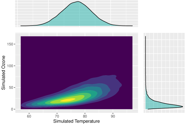
Figure 3: Contour plot and marginal densities for the simulated bivariate distribution of Air Quality Temperatures and Ozone levels. The simulated points mimic the observed data with respect to both the marginal characteristics and bivariate association.

5 Monte Carlo evaluations

In this section, we conduct MC studies to investigate method performance. Marginal parameter matching is straightforward in our scheme as it is a sequence of univariate inverse probability transforms. This process is both fast and exact. On the other hand, accurate and computationally efficient dependency matching presents a challenge, especially in the HD setting. To evaluate our methods in those respects, we design the following numerical experiments to first assess accuracy of matching dependency parameters in bivariate simulations and then time the procedure in increasingly large dimension $d$.

5.1 Bivariate experiments

We select bivariate simulation configurations to ultimately simulate our motivating discrete-valued RNA-seq example. Thus, we proceed by increasing departure from normality, leading to a multivariate negative binomial (MVNB) model for our motivating data. We begin with empirically evaluating the dependency matching across all three supported correlations — Pearson, Spearman, and Kendall — in identical, bivariate marginal configurations. For each pair of identical margins, we vary the target correlation across $\Omega$, the set of possible admissible values for each correlation type, to evaluate the simulation’s ability to generate all possible correlations. The simulations progress from bivariate normal, to bivariate gamma (non-normal yet continuous), and bivariate negative binomial (non-normal and discrete).

Table 3 lists our identical-marginal, bivariate simulation configurations. We increase the simulation replicates $B$ to visually ensure that our results converge to the target correlations and gauge efficiency. We select distributions beginning with a standard multivariate normal (MVN) as we expect the performance to be exact (up to MC error) for all correlation types. Then, we select a non-symmetric continuous distribution: a standard (rate =1), two-component multivariate gamma (MVG). Finally, we select distributions and marginal parameter values that are motivated by our RNA-seq data, namely values proximal to probabilities and sizes estimated from the data (see RNA-seq data application for estimation details). Specifically, we assume a MVNB with $p_{1}=p_{2}=3\times 10^{-4},r_{1}=r_{2}=4,\rho\in\Omega$.

Table 3: Identical margin, bivariate simulation configurations to evaluate matching accuracy.

Simulation Reps $B$	Correlation Types	Identical-margin 2D distribution
$1,000$	Pearson ($\rho_{P}$)	${\bf Y}\sim MVN(\mu=0,\sigma=1,\rho_{i}),i=1,\ldots,100$
$10,000$	Spearman ($\rho_{S}$)	${\bf Y}\sim MVG(shape=10,rate=1,\rho_{i}),i=1,\ldots,100$
$100,000$	Kendall ($\tau$)	${\bf Y}\sim MVNB(p=3\times 10^{-4},r=4,\rho_{i}),i=1,\ldots,100$

For each of the unique 9 simulation configurations described above, we estimate the correlation bounds and vary the correlations along a sequence of 100 points evenly placed within the bounds, aiming to explore $\Omega$. Specifically, we set correlations $\{\rho_{1}=(\hat{l}+\epsilon),\rho_{2}=(\hat{l}+\epsilon)+\delta,\ldots,\rho_{100}=(\hat{u}-\epsilon)\}$, with $\hat{l}$ and $\hat{u}$ being the estimated lower and upper bounds, respectively, with increment value $\delta$. The adjustment factor, $\epsilon=0.01$, is introduced to handle numeric issues when the bound is specified exactly.

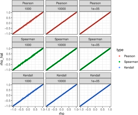
Figure 4: bigsimr recovers the Pearson specified correlations for MVN.

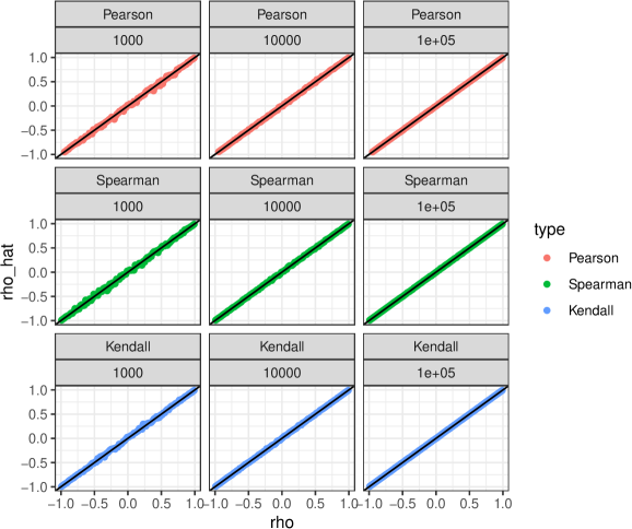
Figure 5: bigsimr recovers the Pearson specified correlations for Bivariate Gamma.

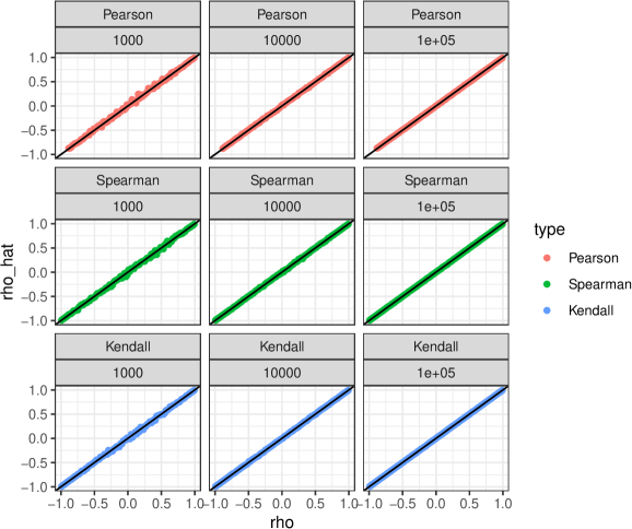
Figure 6: bigsimr recovers the correlations for bivariate negative binomial only approximately for Pearson but (nearly) exactly for the rank-based correlations.

Figure 7 displays the aggregated bivariate simulation results. Table 4 contains the mean absolute error (MAE) in reproducing the desired dependency measures for the three bivariate scenarios. Overall, the studies show that our methodology is generally accurate across the entire range of possible correlation for all three dependency measures. Our Pearson matching performs nearly as well as Spearman or Kendall, except for a slight increase in error for the negative binomial case.

Table 4: Average abolute error in matching the target dependency across the entire range of possible correlations for each bivariate marginal.

No. of random vectors	Correlation type	Distribution	Mean abs. error
1000	Pearson	norm	0.0156184
1000	Pearson	gamma	0.0159287
1000	Pearson	nbinom	0.0162465
1000	Spearman	norm	0.0175440
1000	Spearman	gamma	0.0182176
1000	Spearman	nbinom	0.0151124
1000	Kendall	norm	0.0130284
1000	Kendall	gamma	0.0114740
1000	Kendall	nbinom	0.0126014
10000	Pearson	norm	0.0060226
10000	Pearson	gamma	0.0057667
10000	Pearson	nbinom	0.0058180
10000	Spearman	norm	0.0062388
10000	Spearman	gamma	0.0056132
10000	Spearman	nbinom	0.0049256
10000	Kendall	norm	0.0032618
10000	Kendall	gamma	0.0038067
10000	Kendall	nbinom	0.0033203
1e+05	Pearson	norm	0.0017570
1e+05	Pearson	gamma	0.0016962
1e+05	Pearson	nbinom	0.0029582
1e+05	Spearman	norm	0.0016607
1e+05	Spearman	gamma	0.0016408
1e+05	Spearman	nbinom	0.0015269
1e+05	Kendall	norm	0.0010441
1e+05	Kendall	gamma	0.0011077
1e+05	Kendall	nbinom	0.0011976

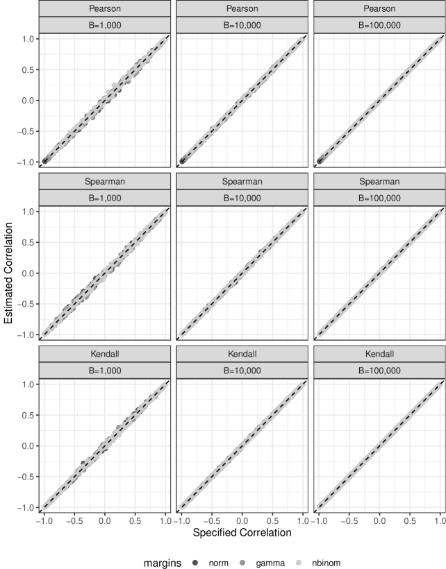
Figure 7: Bivariate simulations match target correlations across the entire range of feasible correlations. The horizontal axis plots the specified target correlations for each bivariate margin. Normal margins are plotted in dark dark grey, gamma in medium grey, and negative binomial in light grey. As the number of simulated vectors $B$ increases from left to right, the variation in estimated correlations (vertical axis) decreases. The dashed line indicates equality between the specified and estimated correlations.

5.2 Scale up to High Dimensions

With information of our method’s accuracy from a low-dimensional perspective, we now assess whether bigsimr can scale to larger dimensional problems with practical computation times. We ultimately generate $B=1,000$ random vectors for $d=\{100,250,500,1000,2500,5000,10000\}$ for each correlation type, {Pearson, Spearman, Kendall} while timing the algorithm’s major steps. We begin by producing a synthetic “data set” by completing the following steps:

1. Produce heterogeneous gamma marginals by randomly selecting the $j^{th}$ gamma shape parameter from $U_{j}\sim uniform(1,10),j=1,\ldots,d$ and the $j^{th}$ rate parameter from $V_{j}\sim exp(1/5),j=1,\ldots,d$, with the constant parameters determined arbitrarily.

2. Produce a random full-rank Pearson correlation matrix via cor_randPD of size $d\times d$.

3. Simulate a “data set” of $1,000\times d$ random vectors via rvec.

With the synthetic data set in hand, we complete and time the following four steps involved in a typical workflow (including correlation estimation).

1. Estimate the correlation matrix from the “data” in the Compute Correlation step.

2. Map the correlations to initialize the algorithm (Pearson to Pearson, Spearman to Pearson, or Kendall to Pearson) in the Adjust Correlation step.

3. Check whether the mapping produces a valid correlation matrix and, if not, find the nearest PD correlation matrix in the Check Admissibility step.

4. Simulate $1,000$ vectors in the Simulate Data step.

The experiments are conducted on a MacBook Pro carrying a 2.4 GHz 8-Core Intel Core i9 processor, with all 16 threads employed during computation. Table 5 displays the total computation time for moderate dimesions ($d\leq 500$). In every simullation setting, the 1,000 vectors are generated rapidly, executing in under 2 seconds.

Table 5: Total time to produce 1,000 random vectors with a random correlation matrix and hetereogeneous gamma margins.

Dimension	Correlation type	Total Time (Seconds)
100	Pearson	0.081
100	Spearman	0.027
100	Kendall	0.075
250	Pearson	0.378
250	Spearman	0.062
250	Kendall	0.375
500	Pearson	1.425
500	Spearman	0.135
500	Kendall	1.495

The results for $d>500$ show scalability to ultra-high dimensions for all three correlation types, although the total times do become much larger. Figure 8 displays computation times for $d=\{1000,2500,5000,10000\}$. For $d$ equal to 1000 and 2500, the total time is under a couple of minutes. At $d$ of 5000 and 10,000, Pearson correlation matching in the Adjust Correlation step becomes costly. Interestingly, Pearson is actually faster than Kendall for $d=10,000$ due to bottlenecks in Compute Correlation and Check Admissibility. Uniformly, matching Spearman correlations is faster, with total times under 5 minutes for $d=10,000$, making Spearman the most computationally-friendly dependency type for our package. With this in mind, we scaled the simulation to $d=20,000$ for the Spearman type and obtained the 1,000 vectors in under an hour (data not shown). In principle, this would enable the simulation of an entire human-derived RNA-seq data set. We note that for a given target correlation matrix and margins, steps 1, 2, and 3 only need to be computed once and the fourth step, Simulate Data, is nearly instaneous for all settings considered.

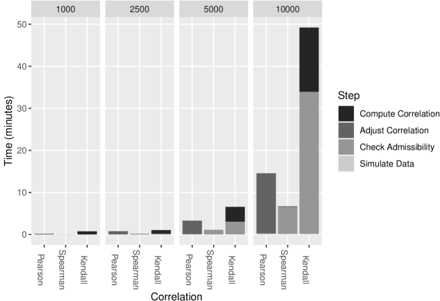
Figure 8: Computation times for HD multivariate gamma simulation.

Limitations, conclusions, and recommendations

In the bivariate studies, we chose arbitrary simulation parameters for three distributions, moving from the Gaussian to discrete and non-normal MVNB. Under these conditions, the simulated random vectors sample the desired bivariate distribution across the entire range of pairwise correlations for the three dependency measures. The simulation results could differ for other choices of simulation settings. Specifying extreme correlations near the boundary or Frechet bounds could result in poor simulation performance. Fortunately, it is straightforward to evaluate simulation performance by using strategies similar to those completed above. We expect our random vector generation to perform well for the vast majority of NORTA-feasible correlation matrices, but advise to check the performance before making inferences/further analyses.

Somewhat surprisingly, Kendall estimation and nearest PD computation scale poorly compared to Spearman and, even, approximate Pearson matching. In our experience, Kendall computation times are sensitive to the number of cores, benefiting from multi-core parallelization. This could mitigate some of the current algorithmic/implementation shortcomings. Despite this, Kendall matching is still feasible for most HD data sets. Finally, we note that one could use our single-pass algorithm cor_fastPD to produce a ‘close’ (not nearest PD) to scale to even higher dimensions with some loss of accuracy.

6 RNA-seq data application

This section demonstrates how to simulate multivariate data using bigsimr, aiming to replicate the structure of HD dependent count data. In an illustration of our proposed methodology, we seek to simulate RNA-sequencing data by producing simulated random vectors mimicking the observed data and its generating process. Modeling RNA-seq using multivariate probability distributions is natural as inter-gene correlation occurs during biological processes (Wang, Gerstein, and Snyder 2009). And yet, many models do not account for this, leading to major disruptions to the operating characteristics of statistical estimation, testing, and prediction. The following subsections apply bigsimr’s methods to real RNA-seq data, including replicating an estimated parametric structure, probability estimation, and evaluation of correlation estimation efficiency.

6.1 Simulating High-Dimensional RNA-seq data

d <- 1000

brca1000 <- example_brca %>%

  select(all_of(1:d)) %>%

  mutate(across(everything(), as.double))

We begin by estimating the structure of the TCGA BRCA RNA-seq data set. Ultimately, we will simulate $B=10,000$ random vectors ${\bf Y}=(Y_{1},\ldots,Y_{d})^{\top}$ with $d=1000$. We assume a MVNB model as RNA-seq counts are often over-dispersed and correlated. Since all $d$ selected genes exhibit over-dispersion (data not shown), we proceed to estimate the NB parameters $(r_{i},p_{i}),i=1,\ldots,d$, to determine the target marginal PMFs $f_{i}$. To complete specification of the simulation algorithm inputs, we estimate the Spearman correlation matrix $R_{S}$ to characterize dependency. With this goal in mind, we first estimate the desired correlation matrix using the fast implementation provided by bigsimr:

# Estimate Spearman's correlation on the count data

R_S <- bs$cor(as.matrix(brca1000), bs$Spearman)

Next, we estimate the marginal parameters. We use the method of moments to estimate the marginal parameters for the multivariate negative binomial model. The marginal distributions are from the same probability family (NB), yet they are heterogeneous in terms of the parameters probability and size $(p_{i},n_{i})$ for $i,\ldots,d$. The functions below support this estimation for later use in rvec.

make_nbinom_margins <- function(sizes, probs) {

  margins <- lapply(1:length(sizes), function(i) {

    dist$NegativeBinomial(sizes[i], probs[i])

  })

  do.call(c, margins)

}

We apply these estimators to the highest-expressing r d genes across the r nrow(brca1000) patients:

mom_nbinom <- function(x) {

  m <- mean(x)

  s <- sd(x)

  c(size = m^2 / (s^2 - m), prob = m / s^2)

}

nbinom_fit <- apply(brca1000, 2, mom_nbinom)

sizes <- nbinom_fit["size",]

probs <- nbinom_fit["prob",]

nb_margins <- make_nbinom_margins(sizes, probs)

Notably, the estimated marginal NB probabilities $\{\hat{p}_{i}\}$ are small — ranging in the interval $[rmin(probs),rmax(probs)]$. This gives rise to highly variable counts and, thus, less restriction on potential pairwise correlation pairs. Given the marginals, we now specify targets and check admissibility of the specified correlation matrix.

# 1. Mapping step first

R_X <- bs$cor_convert(R_S, bs$Spearman, bs$Pearson)

# 2a. Check admissibility

(is_valid_corr <- bs$iscorrelation(R_X))

## [1] FALSE

# 2b. compute nearest correlation

if (!is_valid_corr) {

  R_X_pd <- bs$cor_nearPD(R_X)

  ## Quantify the error

  targets      <- R_X[lower.tri(R_X, diag = FALSE)]

  approximates <- R_X_pd[lower.tri(R_X_pd, diag = FALSE)]

  R_X          <- R_X_pd

}

summary(abs(targets - approximates))

##      Min.   1st Qu.    Median      Mean   3rd Qu.      Max.
## 0.0000000 0.0001929 0.0004129 0.0005064 0.0007168 0.0069224

As seen above, $R_{X}$ is not strictly admissible in our scheme. This can be seen from the negative result from bs$iscorrelation(R_X), which checks if $R_{X}$ is positive-definite with 1’s along the diagonal. However, the approximation is close with a maximum absolute error of r max( abs(targets - approximates)) and average absolute error of r mean(abs(targets - approximates)) across the r choose(d,2) correlations. With the inputs configured, rvec is executed to produce a synthetic RNA-seq data set:

sim_nbinom <- bs$rvec(10000, R_X, nb_margins)

Figure 9 displays the simulated counts and pairwise relationships for our example genes from Table 1. Simulated counts roughly mimic the observed data but with a smoother appearance due to the assumed parametric form and with less extreme points than the observed data in Figure 1. Figure 10 compares the specified target parameter (horizontal axis) with the corresponding quantities estimated from the simulated data (vertical axis). The evaluation shows that the simulated counts approximately match the target parameters and exhibit the full range of estimated correlations from the data.

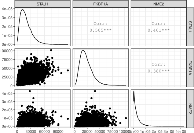
Figure 9: Simulated data for three selected high-expressing genes generally replicates the estimated data structure. The data do not exhibit outlying points, but do possess the desired Spearman correlations, central tendencies, and discrete values.

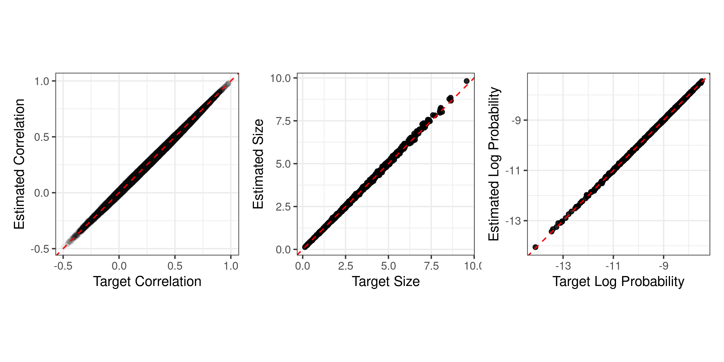
Figure 10: Simulated random vectors from a multivariate negative binomial replicate the estimated structure from an RNA-seq data set. The dashed red lines indicate equality between estimated parameters from simulated data (vertical axes) and the specified target parameters (horizontal axes).

Limitations, conclusions, and recommendations

The results show overall aquedate simulation performance for our choice of parameters settings. Our settings were motivated by modeling high-expressing genes from the TCGA BRCA data set. In general, the ability to match marginal and dependence parameters depends on the particular joint probability model. We recommend to evaluate and tune your simulation until you can be assured of the accuracy.

7 Conclusion and discussion

We developed a general-purpose high-dimensional multivariate simulation algorithm and provide a user-friendly, high-performance R package bigsimr, Julia package Bigsimr and Python package bigsimr. The random vector generation method is inspired by NORTA (Cario and Nelson 1997) and Gaussian copula-based approaches Xiao (2017). The major contributions of this work are methods and software for flexible, scalable simulation of HD multivariate probability distributions with broad data analytic applications for modern, big-data statistical computing. For example, one could simulate high-resolution time series data, such as those consistent with an auto-regressive moving average model exhibiting a specified Spearman structure. Our methods could also be used to simulate sparsely correlated data, as many HD methods assume, via specifying a spiked correlation matrix.

There are limitations to the methodology and implementation. We could only investigate selected multivariate distributions in our Monte Carlo studies. There may be instances where the methods do not perform well. Along those lines, we expect that correlation values close to the boundary of the feasible region could result in algorithm failure. Another issue is that for discrete distributions, we use continuous approximations when the support set is large. This could limit the scalability/accuracy for particular discrete/mixed multivariate distributions. Our method would also benefit computationally from faster Kendall estimation and more finely tuned nearest PD calculation for non-admissible Kendall matrices.

reBarbiero, Alessandro, and Pier Alda Ferrari. 2017. “An R package for the simulation of correlated discrete variables.” Communications in Statistics - Simulation and Computation 46 (7): 5123–40. https://doi.org/10.1080/03610918.2016.1146758.

preCario, Marne C., and Barry L. Nelson. 1997. “Modeling and generating random vectors with arbitrary marginal distributions and correlation matrix.” Technical Report.

preChambers, J. M., W. S. Cleveland, B. Kleiner, and P. A. Tukey. 1983. Graphical Methods for Data Analysis. Belmont, CA: Wadsworth & Brooks.

preChen, Huifen. 2001. “Initialization for NORTA: Generation of random vectors with specified marginals and correlations.” INFORMS Journal on Computing 13 (4): 312–31.

preChernick, Michael R. 2008. Bootstrap Methods: A Guide for Practitioners and Researchers. 2nd ed. Hoboken, NJ.

preConesa, Ana, Pedro Madrigal, Sonia Tarazona, David Gomez-Cabrero, Alejandra Cervera, Andrew McPherson, Michal Wojciech Szcześniak, et al. 2016. “A survey of best practices for RNA-seq data analysis.” https://doi.org/10.1186/s13059-016-0881-8.

preDemirtas, Hakan, and Donald Hedeker. 2011. “A practical way for computing approximate lower and upper correlation bounds.” American Statistician 65 (2): 104–9. https://doi.org/10.1198/tast.2011.10090.

preEfron, Bradley. 2007. “Correlation and large-scale simultaneous significance testing.” Journal of the American Statistical Association 102 (477): 93–103. https://doi.org/10.1198/016214506000001211.

preFasiolo, Matteo. 2016. An introduction to mvnfast. R package version 0.1.6. https://cran.r-project.org/package=mvnfast.

preGhosh, Soumyadip, and Shane G Henderson. 2002. “Properties of the Norta method in higher dimensions.” Proceedings of the 2002 Winter Simulation Conference, 263–69.

preHigham, Nicholas J. 2002. “Computing the Nearest Correlation Matrix—a Problem from Finance.” IMA Journal of Numerical Analysis 22 (3): 329–43.

preKruskal, William H. 1958. “Ordinal measures of association.” Journal of the American Statistical Association 53 (284): 814–61. https://doi.org/10.1080/01621459.1958.10501481.

preLi, Shing Ted, and Joseph L. Hammond. 1975. “Generation of pseudorandom numbers with specified univariate distributions and correlation coefficients.” IEEE Transactions on Systems, Man and Cybernetics 5: 557–61. https://doi.org/10.1109/TSMC.1975.5408380.

preLi, Xiang, A. Grant Schissler, Rui Wu, Lee Barford, Jr. Harris, Fredrick C., and Frederick C. Harris. 2019. “A Graphical Processing Unit accelerated NORmal to Anything algorithm for high dimensional multivariate simulation.” Advances in Intelligent Systems and Computing, 339–45. https://doi.org/10.1007/978-3-030-14070-0_46.

preMadsen, L., and D. Birkes. 2013. “Simulating dependent discrete data.” Journal of Statistical Computation and Simulation 83 (4): 677–91. https://doi.org/10.1080/00949655.2011.632774.

preMari, Dominique Drouet, and Samuel Kotz. 2001. Correlation and dependence. World Scientific.

preMuino, JM, Eberhard O Voit, and Albert Sorribas. 2006. “GS-Distributions: A New Family of Distributions for Continuous Unimodal Variables.” Computational Statistics and Data Analysis 50 (10): 2769–98.

preNelsen, Roger B. 2007. An Introduction to Copulas. 2nd ed. New York: Springer Science & Business Media.

preNikoloulopoulos, Aristidis K. 2013. “Copula-based models for multivariate discrete response data.” In Lecture Notes in Statistics: Copulae in Mathematical and Quantitative Finance, 213th ed., 231–49. Heidelberg: Springer.

prePark, Chul Gyu, Taesung Park, and Dong Wan Shin. 1996. “A simple method for generating correlated binary variates.” American Statistician 50 (4): 306–10. https://doi.org/10.1080/00031305.1996.10473557.

preQi, Houduo, and Defeng Sun. 2006. “A Quadratically Convergent Newton Method for Computing the Nearest Correlation Matrix.” SIAM Journal on Matrix Analysis and Applications 28 (2): 360–85.

preSchissler, Alfred Grant, Dillon Aberasturi, Colleen Kenost, and Yves A. Lussier. 2019. “A Single-Subject Method to Detect Pathways Enriched With Alternatively Spliced Genes.” Frontiers in Genetics 10 (414). https://doi.org/10.3389/fgene.2019.00414.

preSchissler, Alfred Grant, Walter W Piegorsch, and Yves A Lussier. 2018. “Testing for differentially expressed genetic pathways with single-subject N-of-1 data in the presence of inter-gene correlation.” Statistical Methods in Medical Research 27 (12): 3797–3813. https://doi.org/10.1177/0962280217712271.

preÚbeda-Flores, Manuel, and Juan Fernández-Sánchez. 2017. “Sklar’s theorem: The cornerstone of the Theory of Copulas.” In Copulas and Dependence Models with Applications. https://doi.org/10.1007/978-3-319-64221-5_15.

preWang, Zhong, Mark Gerstein, and Michael Snyder. 2009. “RNA-Seq: A revolutionary tool for transcriptomics.” https://doi.org/10.1038/nrg2484.

preXiao, Qing. 2017. “Generating correlated random vector involving discrete variables.” Communications in Statistics - Theory and Methods 46 (4): 1594–1605. https://doi.org/10.1080/03610926.2015.1024860.

preXiao, Qing, and Shaowu Zhou. 2019. “Matching a correlation coefficient by a Gaussian copula.” Communications in Statistics - Theory and Methods 48 (7): 1728–47. https://doi.org/10.1080/03610926.2018.1439962.

preYan, Jun. 2007. “Enjoy the joy of copulas: with a package copula.” Journal of Statistical Software 21 (4): 1–21. http://www.jstatsoft.org/v21/i04.

p