Fairness, Integrity, and Privacy in a Scalable Blockchain-based Federated Learning System

Abstract

Federated machine learning (FL) allows to collectively train models on sensitive data as only the clients’ models and not their training data need to be shared. However, despite the attention that research on FL has drawn, the concept still lacks broad adoption in practice. One of the key reasons is the great challenge to implement FL systems that simultaneously achieve fairness, integrity, and privacy preservation for all participating clients. To contribute to solving this issue, our paper suggests a FL system that incorporates blockchain technology, local differential privacy, and zero-knowledge proofs. Our implementation of a proof-of-concept with multiple linear regression illustrates that these state-of-the-art technologies can be combined to a FL system that aligns economic incentives, trust, and confidentiality requirements in a scalable and transparent system.

Highlights

• Fairness, integrity, and privacy are important requirements for federated learning.

• It is challenging to achieve all of these requirements at the same time.

• With blockchain, differential privacy, and zero-knowledge proofs we can satisfy them.

• We provide a proof of concept for the case of multiple linear regressions.

• Our evaluation indicates that the architecture is practical and scalable.

1 Introduction

The application of machine learning (ML) promises far-reaching potentials across industries [1]. ML has already proven successful in many areas, such as web search or recommender systems in e-commerce, in which a lot of high-quality data exists [2]. While researchers address ML’s growing demand for compute power and use of data with, e.g., distributed ML approaches where multiple computing nodes share their resources [3, 4, 5] and quality issues with data processing, access to data is not only a technical issue. Both traditional ML and distributed ML approaches assume that their training data is centralized by nature, preventing the applicability of ML approaches to domains in which data is sensitive and distributed at the same time. To avoid that ML approaches must rely on data to which only a centralized organization or individual has full access, federated machine learning (FL) can aggregate the less sensitive ML models that were independently and locally trained by individual clients [6, 7]. Consequently, FL can enable the use of ML applications in domains with strong privacy requirements and contribute to solving the challenge of limited access to sensitive data without invading participating clients’ privacy [8, 9]. For instance, researchers at Google aimed to improve next word predictions for mobile devices based on private user data, i.e., the words users are typing [10]. In the case of autonomous driving, FL could reduce the data transmission overhead in vehicular networks while still respecting privacy requirements [11]. These examples demonstrate FL’s capability to avoid the obligation to centralize data. Thus, FL approaches improve functionality or even enable new value creation scenarios for ML.

Despite these promising applications and developments, FL in practice has not yet encountered broad adoption [12]. This can be traced to a variety of design requirements that have not been met simultaneously so far. For example, FL systems require, amongst others, privacy guarantees exceeding FL’s privacy by design [13] as well as high degrees of fairness and integrity [12, 14]. Compared to centralized ML, FL already ensures a certain level of privacy for participating clients [12]. However, even when replacing centralized data with clients’ model updates in a FL system, these public model updates can still leak insights on private client data [13, 15, 16, 17, 18, 19]. While research has addressed this issue with different approaches, there are tradeoffs in terms of performance and integrity, as plausibility checks of the contributed models cannot be made any more when the individual model updates are obfuscated. Second, FL systems can be subject to malicious client attacks that try to harm the global model performance by submitting model updates that have been trained on data sets unequal to the client’s actual data (or even generated on purpose to harm the quality of the aggregate global model). So-called data-poisoning attacks can reduce model performance by up to 90 % [9, 12]. Third, the above application examples assume that users contribute their data, computation, and communication resources unconditionally. However, scaling FL to broad adoption in practice requires fair and transparent incentive mechanisms to appropriately remunerate clients for their contribution to the global model performance [4, 12, 14, 20, 21]. FL can be subject to free-riding attacks in which malicious clients fraudulently benefit from the incentive mechanism by submitting model updates that are not based on the respective client’s private data [12, 14]. Moreover, in a conventional FL setting, clients are forced to trust the central entity to remunerate all clients fairly without being able to check whether this central entity acts truthfully or maliciously.

Satisfying the described privacy, integrity, and fairness requirements in a FL system whilst still being scalable requires an interdisciplinary discourse that bundles up a combination of technologies within a FL system [4, 6]. Even though a vast amount of research in various disciplines already exists, there are, to the best of our knowledge, no systems that jointly deliver privacy, integrity, and fair incentives. Thus, we explore the following research question:
[2em]2em How can a FL system achieve fairness, integrity, and privacy whilst still being practical and scalable?

To answer this research question, we propose a FL system that levers blockchain technology, local differential privacy (LDP), and zero-knowledge proofs. We thus integrate these emerging technologies to provide a novel and smart FL-based architecture with the following properties:

• Fair incentives: Our proposed FL architecture measures the individual contribution to the global model performance per client based on the client’s actual parameters (i.e., without the LDP-noise) and incentivizes each client accordingly. By building our FL system based on blockchain, a smart contract enforces the transparent and verifiable distribution of incentives [22, 23].

• Integrity: Non-interactive ZKPs enable clients to validate that fellow clients have truthfully trained their submitted model updates based on private data that they committed to earlier, potentially including a proof of provenance (e.g., from a certified sensor). In doing so, these fellow clients do not have to reveal any of their private data, yet we can guarantee that they do the training and evaluation for their incentive truthfully. Further, we build our FL system based on blockchain. In the resulting decentralized setting, there is no trust in a central authority needed regarding censorship and the correct aggregation as well as the availability of the global model. Research has already pointed out that a blockchain can be a suitable replacement for intermediaries in a collaborative process and help achieve standardized communication between participants [24]. Besides, the blockchain-based design ensures neutrality amongst all clients, the immutability of transactions, and the full transparency of the architecture for all clients.

• Privacy: To make sure that clients’ model updates cannot leak information on patterns within their private data, we leverage LDP to perturb each clients’ model update with Laplacian noise.

We discuss and instantiate our architecture for multiple linear regression (LR) as FL model. For the implementation, we use succinct non-interactive arguments of knowledge implemented in circom and snarkjs as well as smart contracts deployed on an Ethereum virtual machine (EVM) implemented in Solidity. Through implementing and testing the system, we demonstrate that a realization of our architecture can achieve reasonable performance and scalability. Moreover, we gain valuable insights into how the combination of FL, LDP, ZKPs, and blockchain can be applied to more sophisticated ML models beyond FL. By proposing our FL system that integrates several emerging technologies in a novel way, we contribute a solution that demonstrates that fairness, integrity, and privacy requirements can be solved in practical settings and thus also improve the real-world applicability of existing FL approaches. As we pointed out that using FL approaches alone is not practical for some application scenarios, we contribute to overcoming relevant hurdles towards applicability. The developed FL system is scalable, ensures integrity, and attracts clients to participate through fair incentives as well as data privacy guarantees.

We structure this paper as follows: In Section 2, we briefly present the technical building blocks of our FL system (i.e., FL, LDP, ZKPs, and blockchain technology) and discuss related work on the design of FL systems. Afterward, we present the architecture and implementation of our FL-system in Section 3 and evaluate it in Section 4. Finally, we discuss our results, describe our research’s limitations, and outline future research opportunities in Section 5.

2 Foundations

2.1 Federated Learning

FL describes the concept of training local ML models on distributed and private client data without transferring the data beyond the client’s reach. After training the local parameters, clients in the FL system submit model updates derived from their locally trained parameters to a server that aggregates all local model updates to a global model [4]. The types of potential clients are diverse and range from organizations and mobile devices equipped with sensors to autonomous vehicles. Research has recently applied FL systems in several domains including health, the internet of things (IoT), vehicular networks, finance, sales, or smart homes [6, 9]. By bringing the computation to the data, FL improves clients’ privacy [6]. Besides, FL can increase the efficiency of existing infrastructure and devices by avoiding the transfer of large data sets to a central server and by utilizing the computational power of edge devices like smartphones or wearables [21]. In doing so, FL is typically associated with the following optimization problem [6]:

$$\min\limits_{w_{g}}F(w_{g})=\min\limits_{w_{g}}\left(\sum\limits_{i=1}^{|I|}b_{i}F_{i}(w_{g})\right)~{}\text{,}$$ (1)

where $|I|$ is the total number of clients, $b_{i}\geq 0$, $\sum_{|I|}b_{i}=1$ denotes the client’s relative impact, and $F_{i}(w)$ is the local objective function. The global, aggregated weight $w_{g}$ is mostly derived from the local updates $w_{i}$ using federated averaging (FedAvg), an aggregation scheme that computes a weighted average of the local weights $w_{i}$ [25]. When training on independent and identically distributed (i.i.d.) data, FedAvg achieves similar results to centralized learning [25].

2.2 Local Differential Privacy

Differential privacy (DP) has been developed by Dwork et al. [26] to allow for analyzing sensitive and private data in a secure way: Consider a trusted central authority that holds a data set containing sensitive client information. The key idea of DP is to develop a query function on the sensitive data set that returns the true answer plus random noise following a carefully chosen distribution [27]. For example, in a study that asks participants to report a certain personal property, participants report their binary answer by tossing a coin: They respond truthfully if tails and if heads, the participants toss the coin again and report “yes” if heads and “no” if tails. In this simple example, the participants’ privacy stems from the plausible deniability of any reported value [27].

The driving force for this privacy guarantee is randomization since the guarantee must hold regardless of all present or even future sources of background information (e.g., from the internet or newspapers). Achieving this requires understanding the input and output space of randomized algorithms. Formally, a randomized algorithm $\mathcal{M}$ with domain $A$ and (discrete) range $B$ is associated with a mapping from $A$ to $\Delta(B)$, the probability simplex over $B$:

$$\Delta(B)=\Bigg{\{}x\in\mathbb{R}^{|B|}:x_{i}\geq 0~{}\mathrm{for~{}all}~{}i~{}\mathrm{and}~{}\sum\limits_{i=1}^{|B|}x_{i}=1\Bigg{\}}.$$ (2)

Then, on input $a\in A$ and given that the probability space is over the coin flips of $\mathcal{M}$, the randomized algorithm $\mathcal{M}$ outputs $\mathcal{M}(a)=b$ with probability $\left(\mathcal{M}(a)\right)_{b}$ for every $b\in B$ [27]. Before defining DP, note that DP aims to sanitize a query function such that the presence or absence of an individual in the analyzed data set cannot be determined by just observing the output of the query. Now consider two data sets $D$ and $D^{\prime}$, that are either equal or differ only in the presence or absence of one individual, as histograms. Moreover, a histogram over a universe $\mathcal{X}$ is an object in $\mathbb{N}^{\mathcal{|X|}}$. Then, both data sets $D,D^{\prime}\in\mathbb{N}^{\mathcal{|X|}}$ are called adjacent if for the $\ell_{1}$-norm, $\lVert D-D^{\prime}\rVert_{1}\leq 1$ holds. Eventually, Dwork et al. [26] define DP as follows:

Definition.

A randomized algorithm $\mathcal{M}$ with domain $\mathbb{N}^{\mathcal{|X|}}$ and range $\mathcal{R}$ satisfies $\epsilon$-differential privacy if for every adjacent data sets $D,D^{\prime}\in\mathbb{N}^{\mathcal{|X|}}$ and any subset $\mathcal{S}\subseteq\mathcal{R}$ we have

$$\mathrm{Pr}[\mathcal{M}(D)\in\mathcal{S}]\leq e^{\epsilon}~{}\mathrm{Pr}[\mathcal{M}(D^{\prime})\in\mathcal{S}],$$ (3)

where $\epsilon>0$ is a privacy parameter.

A common way to achieve DP for a numeric function $f$ is to add noise following a Laplacian distribution:

$$\mathcal{L}(x~{}|~{}0,\lambda) =\frac{1}{2\lambda}\exp{\left(-\frac{|x|}{\lambda}\right).}$$ (4)

When a user wants to learn $f(\mathbf{x})=\sum_{i}x_{i}$ with $\mathbf{x}\in\{0,1\}$, i.e., the total number of 1’s in the data set, $\epsilon$-DP can be achieved by adding Laplacian noise [27, 28]:

$$\tilde{f}(\mathbf{x})=\sum_{i}x_{i}+q,\qquad\mathrm{where}~{}q\sim\mathcal{L}\left(0,\frac{\Delta f}{\epsilon}\right).$$ (5)

and $\Delta f$ denotes the sensitivity of $f$, i.e., the maximum difference of $f$ on data sets that differ in only one element [28]. There are many practical algorithms for providing DP; and in general, they have many characteristics beyond $\varepsilon$ that have an impact on privacy or utility [29]. One special case of DP is local differential privacy (LDP), where the confusion (i.e., random perturbation) is performed locally by clients and not by a central authority [30]. By doing so, the central authority cannot infer or access the actual client data. According to Definition Definition, anyone accessing $\mathcal{S}$ cannot distinguish whether the true data set is $D$ or $D^{\prime}$ with confidence (controlled by $\epsilon$ – the lower $\epsilon$, the higher the privacy and the lower the accuracy and vice versa). Thus, LDP ensures plausible deniability for the clients [31].

2.3 Verifiable Computation and Zero-Knowledge Proofs

The notion of ZKPs was first introduced by Goldwasser et al. [32]. ZKPs are a special form of protocols between a so-called prover and a verifier in which the prover wants to convince the verifier that she/he knows some value with a specific property (more formally, an element of a language). ZKPs have the additional property that the prover learns nothing beyond this statement. The most important properties beyond zero-knowledgeness that we build upon in this paper are completeness (an honest prover will convince the verifier with high probability if the statement is correct) and soundness (any and in particular a malicious prover will convince the verifier of a false statement only with a small probability). By replacing the verifier with a random oracle such as a hash function, a large class of interactive proofs can be transferred to non-interactive proofs (using the so-called Fiat-Shamir heuristic [33]). As opposed to interactive ZKPs, prover and verifier do not have to interact with each other in non-interactive ZKPs. Notably, there are succinct ZKP, which means that both the proof size as well as the computational complexity of the proof verification is considerably smaller than the complexity of checking the statement by conducting the original computation [34].

Since the introduction of ZKP, there has been a lot of research on them, but practical implementations or even applications remained rare before the beginning of the 2010s. However, starting with Groth et al. [35], a period of rapid development of ZKP towards practical implementations delivered significant performance improvements, e.g., in [36]. In recent years, different flavors of non-interactive ZKPs have emerged, for example, Bulletproofs [37], SNARKs [38], scalable transparent arguments of knowledge [39], or hybrid constructions. While they differ in scaling properties and cryptographic assumptions, they all allow creating proofs for the correct execution of a program without displaying all inputs, outputs or intermediate steps. Often, Merkle proofs for the inputs are revealed to commit the prover to the usage of unknown but fixed variables. Domain-specific languages such as Circom or Cairo allow compiling programs into arithmetic circuits. From these, polynomials are constructed, which in turn can be translated into proving and verification programs through libraries such as libsnark or snarkjs. As such generic tools for ZKP have significantly matured over the last years, they have increasingly been used in first applications; often associated with blockchains and distributed ledgers, where due to redundant execution, cheap verification without revealing sensitive data is important [39]. However, the generality to which the correctness of computations can be proved with these frameworks is often limited to prime field operations, complemented by libraries that provide, e.g., circuits for basic cryptographic and arithmetic operations such as hash functions, signature schemes, and comparators.

2.4 Blockchains and Distributed Ledger Technology

Blockchain and, more general, distributed ledger technology builds upon peer-to-peer networks in which all data is replicated, shared, and distributed across multiple servers (‘nodes’) [40]. In blockchains, an append-only structure connects batches of transactions (‘blocks’) linearly through hash-pointers (‘chain’) and thus achieves decentralized yet synchronized data management. A so-called consensus mechanism that typically combines cryptographic techniques with economic or social incentives allows deciding which blocks to append as well as the order of transactions within a block [41]. If a majority of the network in a specific metric like hash rate (proof of work), the share of cryptocurrency (proof of stake), or the number of accounts in a permissioned network (voting-based consensus mechanisms) is honest, this guarantees the correct execution of simple payments and programming logic (“smart contracts”) and the practical immutability of the ledger [41]. The confidence that a majority of the network behaves as intended without the need to rely on the honesty of a distinguished entity is often referred to as digital trust [42]. Consequently, blockchains allow avoiding dependencies on one or a few distinct entities on digital platforms [43, 44]. The literature distinguishes between permissionless blockchains (such as those used in cryptocurrencies) where anyone can participate and permissioned blockchains where participation is limited, e.g., to an industry consortium or the public sector [45].

Since the release of the Bitcoin whitepaper [46], blockchain technology has been used in various applications, e.g., cryptocurrencies, decentralized finance with derivatives and non-fungible tokens, or industry applications. One early and popular permissionless blockchain that supports a Turing-complete programming language for smart contracts is Ethereum. It provides a decentralized virtual machine environment, namely the Ethereum virtual machine (EVM), for executing smart contracts. Ethereum smart contracts are usually implemented in Solidity, a high-level programming language with syntax similar to JavaScript [47]. Two special properties of Solidity are the lack of non-deterministic libraries (that would otherwise conflict with the necessarily deterministic design of a blockchain that first orders and then executes transactions) and that the complexity of execution has a price, counted in so-called gas. This avoids not only infinite loops but facilitates fair competition for the limited capacity.

However, as blockchains and distributed ledgers exhibit redundant storage and computation, they suffer from major challenges. While a high energy consumption is often presumed, in fact, only proof of work blockchains are problematic in this regard [48]. Two other issues that arise directly from replicated transaction storage and execution are considerably more fundamental: Scalability [49] and privacy [50]. Yet, there are innovative approaches to mitigate these challenges. For scalability, countermeasures range from restricting participation and demanding high computational power, storage, and bandwidth from the participating nodes to sharding and off-chain computations. Off-chain computations are also good for privacy, but lead to the challenge of verification in a system with malicious participants. On the other hand, methods for privacy are technologies like LDP, fully homomorphic encryption (FHE), or multiparty computation (MPC) [51]. ZKPs can be regarded as a special case of verifiable MPC where only one participant contributes private data but the result is verified by all blockchain nodes. Yet, ZKPs are arguably significantly closer to broad adaption and have been leveraged by many blockchain projects so far, starting with Z-Cash and now also covering many scalability and privacy projects, many of which are implemented on Ethereum (e.g., Tornado-Cash, Loopring, Aztec, StarkDEX).

2.5 Related Work

Since the term federated machine learning was introduced by McMahan et al. [52], research has focused on improving, amongst others, performance, privacy, integrity, and incentive-mechanisms [12, 14]. To improve the clients’ privacy beyond the level that FL inherently offers, research came up with three main strategies, namely homomorphic encryption, MPC, and DP, which aim to prevent public model updates from leaking private client information. Due to its low complexity and strong privacy guarantee [4], DP is widely used [6], even though deploying DP in ML leads to a trade-off between maximizing privacy (i.e., adding noise with high variance) and maximizing accuracy. In practice, instead of uploading the actual weights, clients can add DP noise to their weights. For example [53] developed a FL system for vehicular networks that combines LDP with gradient descent to avoid attacks that leak private information from publicly available ML model updates. Instead of perturbing model parameters, LDP noise can also be added to the training data [7]. However, this approach cannot provide privacy protection since it is not sufficient to make any single record unnoticeable [54].

Besides, many works have adopted game-theoretic approaches to motivate clients’ participation in a FL system and ensure fairness amongst them. As an example, Khan et al. [55] implemented a Stackelberg game to incentivize clients for contributing to training a model and, at the same time, maximize the model’s performance. Since clients must trust the central authority to incentivize all clients fairly in a traditional FL setting and to provide a decentralized incentive layer for data sharing in general [56], researchers have suggested using blockchains and smart contracts for model aggregation (e.g., [57]) and client remuneration (e.g., [58] or [59]). Sun et al. [60] propose a FL architecture that leverages a blockchain for transparency and incentivizing clients and combines it with homomorphic encryption in the aggregation smart contract to prevent leakage from clients’ contributions. However, in all these frameworks, offering incentives to clients also puts the system’s integrity at risk as malicious clients may try to fraudulently benefit from the incentive mechanism, e.g., through free-riding attacks [12, 14].

The transparency of smart contracts could help achieve integrity by allowing clients to recalculate the weights that fellow clients submitted. However, even when ignoring the corresponding privacy and scalability challenges, such an approach would lead to a “verifier’s dilemma” [61], where clients weigh up between accepting the costs of recalculation or trusting other clients. ZKP could offer an efficient solution to the “verifier’s dilemma” in FL and, thus, pave the way to achieving fairness, integrity, and privacy at the same time. Despite ZKPs’ potential for FL systems and their increasing adoption (especially in the blockchain domain), it remains an open question how ZKPs can be used in the context of FL [4]. Wu et al. [62] have implemented a SNARK that proves the correctness of LR parameters by recalculating them. In the case of LR, this can be done only using matrix multiplications. However, this approach includes rounding a matrix inverse and, hence, requires further measures to ensure full tamper protection (as we will show in detail in Section 3.1.1). Feng et al. [63] introduced a toolchain to produce verifiable and privacy-preserving SNARKs that prove correct inference in classification and recognition tasks by taking an existing neural network as input. Also Zhang [64] as well as Weng et al. [65] implemented ZKPs that allow verifying whether a particular prediction by a trained ML model has been computed truthfully without providing any information about the ML model itself. Even though also Weng et al. [65]’s work implements a ZKP merely for ML model inference, they improved ZKPs’ efficiency to prove the correctness of matrix multiplications and ZKPs’ application to floating point arithmetic, which are both essential ingredients for training ML models.

Despite the advancement that these works generate for combining ZKPs and ML, it remains, to the best of our knowledge, still unclear how recent progress in ZKPs, blockchain technology, and DP can be combined as a technology stack that achieves full privacy, integrity, and fairness in FL systems.

3 Architecture and Implementation

We organize Section 3 as follows: In Section 3.1 we explain how our suggested FL system is built up formally. To do so, we divide the FL process into four different sections, namely Compute and Prove Model Weight (Section 3.1.1), Model Aggregation (Section 3.1.2), Compute and Prove Model Cost (Section 3.1.3), and Compute Incentives (Section 3.1.4). Table 1 introduces the notation that we use throughout this section.

Symbol	Explanation
$I$	Set of indices, $i\in\{1,\ldots,\lvert I\rvert\}$
$u_{i}$	Client $i$, $i\in I$
$k$	Number of features of the linear regression
$n$	Sample size per client of the linear regression (set globally)
$d$	Accuracy of rounded inputs
$\mathbf{X}_{i}$	$n\times(k+1)$ Matrix of input data including all independent variables
$Y_{i}$	$n$-dimensional vector of input data containing all dependent variables
$\mathbf{Z}_{i}$	Approximate inverse of $(\mathbf{X}_{i}^{\intercal}\mathbf{X}_{i})^{-1}$
$\mathbf{D}_{i}$	Private data set of $u_{i}$ – an $n\times(k+2)$ matrix: $(X_{i,0},X_{i,1}\ldots X_{i,k}~{}Y_{i})$
$\mathbf{D}_{\textrm{test}}$	Public test data set
$rt^{\mathbf{D}}_{i}$	Merkle tree root of $\mathbf{D}_{i}$
$rt^{\mathbf{D}_{\mathrm{test}}}_{i}$	Merkle tree root of $\mathbf{D}_{\textrm{test}}$
$l_{\mathrm{train}}$	Depth of $\mathbf{D}_{i}$’s Merkle tree (number of levels)
$l_{\mathrm{test}}$	Depth of $\mathbf{D}^{\mathrm{test}}_{i}$’s Merkle tree (number of levels)
$\varepsilon_{\mu}$	Upper bound for $\mu\>\cdot\>n$
$\varepsilon_{\sigma}$	Upper bound for $\sigma\>\cdot\>n$
$\varepsilon_{\mathrm{inverse}}$	Upper bound for $\lVert(\mathbf{X}^{\intercal}\mathbf{X})\mathbf{Z}-\mathbbm{1}\rVert$
$\varepsilon_{w}$	Upper bound for $\lVert w-\tilde{w}\rVert$
$\varepsilon_{w^{\prime}}$	Upper bound for $\lVert w^{\prime}-\tilde{w}^{\prime}\rVert$
$\vartheta_{\mathbf{X}^{\intercal}Y}$	Upper bound for $\lVert\mathbf{X}^{\intercal}Y\rVert$
$\vartheta_{\mathbf{Z}}$	Upper bound for $\lVert\mathbf{Z}\rVert$
$M$	Model (corresponds to respective weight vector)
$w_{i}$	Weight vector of $u_{i}$, corresponding to $M_{i}$
$w_{i}^{\prime}$	Weight vector including LDP noise
$\tilde{w}_{i}$	Recalculated weight vector
$\tilde{w}_{i}^{\prime}$	Recalculated weight vector including LDP noise
$w_{\mathrm{g}}$	Weight vector of global model $M_{\mathrm{g}}$
$\varepsilon_{\mathrm{LR}}$	Error term of LR
$L$	Vector including Laplacian LDP noise
$d_{\mathcal{L}}$	Accuracy of the Laplacian LDP noise
$q$	LDP noise
$h_{j}$	Hash serving as random noise for $q$
$hash\_alg$	Hash algorithm, i.e., $0$ for ‘MiMC’ or $1$ for ‘Poseidon’
$C$	Vector of $u_{i}$’s cost: $(c_{1},\dots,c_{|I|})$
$V$	Vector of $u_{i}$’s incentive payment: $(v_{1},\dots,v_{|I|})$
$B$	Admission fee payable upon joining the system
$\pi(a,b)$	ZKP for statement $a$ with witness $b$
Gen($\pi$)	Construct the ZKP $\pi$ (with the proving key)
Ver($\pi$)	Verify ZKP $\pi$ (with the verification key)

Table 1: Notation used in this paper.

3.1 Conceptual Architecture

3.1.1 Compute and Prove Model Weight

At the start, participating clients $u_{i}$ can register at the smart contract Clients. To do so, they must commit to the Merkle root $rt^{\mathbf{D}}_{i}$ of their private data set $\mathbf{D}_{i}=(\mathbf{X}_{i}~{}Y_{i})=(X_{i,0}~{}X_{i,1}~{}\ldots~{}X_{i,k}~{}Y_{i})\in\mathbb{R}^{n\times(k+2)}\sim\mathbb{R}^{n(k+2)}$ with

$$\mathbf{X}_{i}=\begin{pmatrix}x_{i,0,1}&x_{i,1,1}&\cdots&x_{i,k,1}\\ x_{i,0,2}&x_{i,1,2}&\cdots&x_{i,k,2}\\ \vdots&\vdots&\ddots&\vdots\\ x_{i,0,n}&x_{i,1,n}&\cdots&x_{i,k,n}\end{pmatrix}=\begin{pmatrix}1&x_{i,1,1}&\cdots&x_{i,k,1}\\ 1&x_{i,1,2}&\cdots&x_{i,k,2}\\ \vdots&\vdots&\ddots&\vdots\\ 1&x_{i,1,n}&\cdots&x_{i,k,n}\end{pmatrix}\in\mathbb{R}^{n\times(k+1)}$$

and

$$Y_{i}=\left(y_{i,1},\ldots,y_{i,n}\right)^{\intercal}\in\mathbb{R}^{n}\textrm{.}$$

Prior to computing $rt^{\mathbf{D}}_{i}$ and training their LR weights, clients must normalize their input data $\mathbf{D}_{i}$, such that every $X_{i,1},\ldots,X_{i,k},Y_{i}$ has expectation value $\mu=0$ and standard deviation $\sigma=1$ (in line with, e.g., Witten et al. [66]). Subsequently, clients train their LR weight $w_{i}=(\beta_{i,0}~{}\beta_{i,1}\ldots\beta_{i,k})^{\intercal}\in\mathbb{R}^{k}$ by computing

$$w_{i}=(\mathbf{X}_{i}^{\intercal}\mathbf{X}_{i})^{-1}~{}\mathbf{X}_{i}^{\intercal}~{}Y_{i}.$$ (6)

Equation (6) optimizes

$$\min(\text{RSS})=\min\limits_{w\in\mathbb{R}^{k}}\left((Y_{i}-\mathbf{X}_{i}w_{i})^{\intercal}(Y_{i}-\mathbf{X}_{i}w_{i})\right)=\lVert\varepsilon_{\mathrm{LR},i}\rVert_{2}$$ (7)

where $Y_{i}=\mathbf{X}_{i}w_{i}+\varepsilon_{\mathrm{LR},i}$ and $\varepsilon_{\mathrm{LR},i}$ denotes the LR’s error term. Constructing the ZKP $\pi^{w}$ that ensures that $u_{i}$ computed $w_{i}$ truthfully (i.e., truly computed the $w_{i}$ that minimizes the residual sum of squares (RSS) using (7) based on $u_{i}$’s originally committed data) requires adapting the protocol to circom’s capabilities that are restricted to prime field operations and, thus, to non-negative integer inputs. To do so, we decide to generally round and subsequently scale all (public and private) ZKP inputs $\mathbf{A^{\lvert S\rvert\times\lvert T\rvert}}=(a_{s,t})_{s=1,\ldots,\lvert S\rvert;~{}t=1,\ldots,\lvert T\rvert}$ as in general we cannot assume that $a_{s,t}\in\mathbb{N}_{0}$. For example, we convert the input $a_{s,t}=2.5347725$ to $2.53477\cdot 10^{5}=253477=\tilde{a}_{s,t}$ in the cae of $d=5$. Further, to input only positive integers, we introduce a matrix $\mathbf{Sign(A)}$ whose elements indicate the signs of $\mathbf{A}$’s coefficients: $\left(\mathbf{{Sign}(A)}\right)_{s,t}=\mathrm{sign}(a_{s,t})$ where

$$\mathrm{sign}:\mathbb{Z}\to\{-1,1\},\quad x\mapsto\begin{cases}0&\text{if $x\geq 0$}\\ 1&\text{if $x<0$}\end{cases}.$$

Then we can write the ZKP inputs as

$$\tilde{\mathbf{A}}=10^{-d}\,\mathbf{{Sign}(A)}\circ\mathbf{\tilde{A}^{+}}\qquad\text{where}\quad\tilde{a}^{+}_{s,t}\in\mathbb{N}_{0}\text{.}$$ (8)

Moreover, $\lVert\mathbf{\tilde{A}}-\mathbf{A}\rVert\leq c\cdot 10^{-d}$, where $c$ depends on the choice of matrix norm. For example. if we use the maximum norm, $c$ can be $0.5$ times the number of columns of $A$.

After this transformation, $u_{i}$ can compute the ZKP. However, as constructing proofs is computationally expensive, designing the ZKP generation requires specific consideration and optimizations. For better readability, we will refrain from using client indices $i$ in the following description. First, to make sure that the client’s input data is standardized, we introduce an upper bound for the mean $\mu$. Note that since circom does not allow for non-integer divisions, we apply the upper bound controlling $\mu$ to the sum of all elements in $Y$ and $X_{1},\ldots X_{k}$:

$$\begin{split}\mu_{X_{j}}\cdot n=\sum\limits_{l=1,\ldots n}x_{j,l}&\leq\varepsilon_{\mu}\\ \mu_{Y}\cdot n=\sum\limits_{l=1,\ldots n}y_{l}&\leq\varepsilon_{\mu}\end{split}~{}\quad~{}\forall~{}j\in\{1,\ldots,k\}.$$ (9)

Similarly, we regulate the data set’s variance $\sigma^{2}$ by applying an upper bound to the squared sums:

$$\begin{split}\sigma_{X_{j}}^{2}\cdot n=\sum\limits_{l=1,\ldots n}\left(x_{j,l}-\mu\right)^{2}&\leq\varepsilon_{\sigma}\\ \sigma_{Y}^{2}\cdot n=\sum\limits_{l=1,\ldots n}\left(y_{l}-\mu\right)^{2}&\leq\varepsilon_{\sigma}\end{split}~{}\quad~{}\forall~{}j\in\{1,\ldots,k\}.$$ (10)

Hence, $\varepsilon_{\mu}$ and $\varepsilon_{\sigma}$ must be set with respect to $n$.

Recalling (6), our initial attempt was to compute the inverse $(\mathbf{X}^{\intercal}\mathbf{X})^{-1}$ within a circuit of the respective ZKP by introducing two integers, a denominator and a numerator, per input value. This procedure would allow us to calculate $(\mathbf{X}^{\intercal}\mathbf{X})^{-1}$ in the circuit (as divisions leading to non-integer values can be replaced by multiplications) without rounding errors (given the input values are precise). However, the approach turned out to have one significant shortcoming: Computing $(\mathbf{X}^{\intercal}\mathbf{X})^{-1}$ within a circuit using Gaussian elimination quickly results in overflow (i.e., a numerator or denominator can quickly get larger than the size of the prime field). Finding common denominators often requires multiplying all denominators repeatedly. For example, already computing the inverse of $(\mathbf{X}^{\intercal}\mathbf{X})^{5\times 5}$ matrices with $d=5$ can cause an overflow (in general, this will depend on the choice of $d$ and $k$, but $2^{k}\cdot d$ will probably be larger than $78$ in many practical applications). On the other hand, reducing fractions or rounding (using range proofs) before overflow would add further complexity in the Gaussian elimination algorithm. Besides, more complex operations demanded by more sophisticated ML algorithms would require to hand-craft a fast numerical solver, so the method does not generalize well. Eventually, this approach would hardly scale to more complicated optimization algorithms.

As matrix inversion inside the circuit or inverting within circom’s prime field is expensive, we decided to follow the approach of Wu et al. [62] to solve the problem by letting clients calculate and provide an inverse $\mathbf{Z}\approx(\mathbf{X}^{\intercal}\mathbf{X})^{-1}$ outside the circuit through a standard solver such as typical matrix inversion tools in Javascript, Python, or MATLAB. We then give this inverse as private input to the circuit (again complying with the above-described conversion to non-negative integer entries). However, due to the finite precision of the matrix inversion, we cannot assume that equality holds. Thus, we apply a slightly different method and only prove the proximity of the calculated inverse to the true inverse. To do so, we check the approximation error of the provided numerical inverse using the following range constraint:

$$\lVert(\mathbf{X}^{\intercal}\mathbf{X})\mathbf{Z}-(\mathbf{X}^{\intercal}\mathbf{X})(\mathbf{X}^{\intercal}\mathbf{X})^{-1}\rVert=\lVert(\mathbf{X}^{\intercal}\mathbf{X})\mathbf{Z}-\mathbbm{1}\rVert\leq\varepsilon_{\mathrm{inverse}}<1.$$ (11)

As matrix norm, the maximum norm is a convenient choice, i.e., the inequality can be checked index-wise (respecting $k$). Through this bound, we can both control for the effect that the replacement of $(\mathbf{X}^{\intercal}\mathbf{X})^{-1}$ with its approximation $\mathbf{Z}$ has and ensure that the system remains protected against malicious client attacks. To do so, we estimate an upper bound for the approximation effects on the distance from $w$ to $\tilde{w}$, with the latter being calculated based on $\mathbf{Z}$, via

$$\begin{split}\lVert w-\tilde{w}\rVert&\leq\lVert(\mathbf{X}^{\intercal}\mathbf{X})^{-1}\mathbf{X}^{\intercal}Y-\mathbf{Z}\mathbf{X}^{\intercal}Y\rVert\\ &\leq\lVert(\mathbf{X}^{\intercal}\mathbf{X})^{-1}-\mathbf{Z}\rVert\cdot\lVert\mathbf{X}^{\intercal}Y\rVert\leq\varepsilon_{w},\end{split}$$ (12)

where we use the submultiplicativity of $\lVert\,\cdot\,\rVert$. Even though all entries of $\mathbf{X}^{\intercal}$ and $Y$ are normalized, i.e., $X_{1},\ldots,X_{k},Y$ have expectation value $\mu=0$ and the standard deviation $\sigma=1$, $\lVert\mathbf{X}^{\intercal}Y\rVert$ might still yield large entries. Thus, to control the error $\lVert w-w^{\prime}\rVert$ between the true weights and the client’s approximative result, we desire upper bounds for both $\lVert(\mathbf{X}^{\intercal}\mathbf{X})^{-1}-\mathbf{Z}\rVert$ and $\lVert\mathbf{X}^{\intercal}Y\rVert$.

First, we introduce a simple range proof to ensure that $\lVert\mathbf{X}^{\intercal}Y\rVert$ is bounded:

$$\lVert\mathbf{X}^{\intercal}Y\rVert\leq\vartheta_{\mathbf{X}^{\intercal}Y}\quad\mathrm{where}\quad\vartheta_{\mathbf{X}^{\intercal}Y}\equiv\vartheta_{\mathbf{X}^{\intercal}Y}\left(k,d\right)\text{.}$$ (13)

In general, the probability that $\lVert\mathbf{X}^{\intercal}Y\rVert$ is large is very small as the normal distribution decays fast; if by coincidence a single value is big, $d$ might need to be adjusted to increase the accuracy of rounded inputs.

Second, we recall that the true inverse can essentially be replaced by the approximative inverse as long as the approximate inverse is bounded [67]. More precisely, given any matrix norm $\lVert\,\cdot\,\rVert$, a square nonsingular matrix $\mathbf{A}$ and its approximate inverse $\mathbf{Z}$ such that $\lVert\mathbf{A}\mathbf{Z}-\mathbbm{1}\rVert\leq\varepsilon_{\mathrm{range}}<1$, the bound

$$\lVert\mathbf{A}^{-1}-\mathbf{Z}\rVert\leq\frac{\lVert\mathbf{Z}\rVert\times\lVert\mathbf{A}\mathbf{Z}-\mathbbm{1}\rVert}{1-\lVert\mathbf{A}\mathbf{Z}-\mathbbm{1}\rVert}$$ (14)

holds. However, it is not clear that $\mathbf{X}^{\intercal}\mathbf{X}$ is non-singular, and checking this inside the circuit, e.g., through computing the determinant, would become expensive already for moderate $k$. Fortunately, we can relax the assumption by reconsidering the argument in the derivation of the result in Newman [67]: Provided the candidate for the approximate inverse satisfies $\lVert\mathbf{R}\rVert<1$ for $\mathbf{R}:=\mathbf{A}\mathbf{Z}-\mathbbm{1}$, then the Neumann-series $\mathbbm{1}+\mathbf{R}+\mathbf{R}^{2}+\ldots$ converges. Consequently, using the argument in the paper,

$$\mathbf{A}\mathbf{Z}\cdot(\mathbbm{1}+\mathbf{R}+\mathbf{R}^{2}+\ldots)=(\mathbbm{1}-\mathbf{R})\cdot(\mathbbm{1}+\mathbf{R}+\mathbf{R}^{2}+\ldots)=\mathbbm{1}.$$ (15)

It follows that $\mathbf{Z}(\mathbbm{1}+\mathbf{R}+\mathbf{R}^{2}+\ldots)$ is a right-inverse of the quadratic matrix $\mathbf{A}$ and hence its unique (left- and right-) inverse, i.e., $\mathbf{A}$ is non-singular. In particular, we learn that if $\mathbf{A}$ was non-singular, we could not find an approximate inverse that satisfies (11). Applied to $\mathbf{A}:=\mathbf{X}^{\intercal}\mathbf{X}$, our circuit already implicitly guarantees that $\mathbf{X}^{\intercal}\mathbf{X}$ is invertible through checking (11), and (14) yields

$$\lVert(\mathbf{X}^{\intercal}\mathbf{X})^{-1}-\mathbf{Z}\rVert\leq\frac{\lVert\mathbf{Z}\rVert\times\lVert(\mathbf{X}^{\intercal}\mathbf{X})\mathbf{Z}-\mathbbm{1}\rVert}{1-\lVert(\mathbf{X}^{\intercal}\mathbf{X})\mathbf{Z}-\mathbbm{1}\rVert}\leq\vartheta_{\mathbf{Z}}\cdot\varepsilon_{\mathrm{inverse}}~{}\text{,}$$ (16)

where $\quad\rVert\mathbf{Z}\lVert~{}\leq~{}\vartheta_{\mathbf{Z}}$ and $\vartheta_{\mathbf{Z}}\equiv\vartheta_{\mathbf{Z}}\left(k,d\right)$.

Before uploading $w$ to the EVM storage, clients must perturb their weight by adding Laplacian LDP-noise (recall (4) and (5)) to avoid deep leakage [19]:

$$w^{\prime} =w+q,\qquad q\sim\mathcal{L}(0,\lambda),~{}q\in\mathbb{R}^{k}$$ (17)

$$\lambda =\frac{\Delta}{\epsilon}=\frac{1}{\epsilon}\left(\max\beta_{i,j}-\min\beta_{i,j}\right)\qquad i\in\{1,\dots,\lvert I\rvert\},~{}j\in\{0,\dots,k\}.$$ (18)

Note that every entry in $q$ is drawn separately, following $\mathcal{L}(0,\lambda)$. Moreover, since we perturb client weights that will be aggregated, we must set the LDP security parameter $\epsilon$ globally. As no fellow $\beta_{i,j}$ will be available to any client before uploading the client’s own $w$, we must set an estimation for $\Delta$ globally. Recalling that all $w$ are computed based on normalized data, we know that $\beta_{0},\dots,\beta_{k}\in[\text{-}1;1]$ holds. Therefore, we set $\Delta=2\cdot 10^{d}$ as a proxy. Moreover, to generate $\pi^{w}$, we must ensure that we can reproduce every entry in $q$ while keeping its choice random. Achieving this requires a twofold approach.

First, since circom does not have tools to compute a Laplace-distributed random variable directly, we discretize $\mathcal{L}(0,\lambda)$, introducing a variable $d_{\mathcal{L}}=10^{x}$ with $x\in\mathbb{N}$ that defines the interval of a discrete distribution $\mathcal{DL}(0,\lambda)$ of $\mathcal{L}(0,\lambda)$ (i.e., $\mathcal{DL}$’s accuracy). We then construct a vector $L\in\mathbb{R}^{d_{\mathcal{L}}-1}$ whose entries are given by the inverse cumulative distribution function of $\mathcal{DL}(0,\lambda)$:

$$L(p):=-\lambda~{}\text{sgn}\left(p-\frac{1}{2}\right)~{}\text{ln}\left(1-2\Big{|}p-\frac{1}{2}\Big{|}\right),\quad p=\{1,\dots,d_{\mathcal{L}}-1\}.$$ (19)

The finite nature of machines leads to some form of discretization of distributions, which makes DP mechanisms generally vulnerable to attacks [68]. Therefore, there is a research stream dedicated to exploring the effects of discretization on LDP (e.g., Balcer and Vadhan (2019), Canonne et al. (2021)). However, in our system, the parameters are currently set in a way that the limitation through $d_{\mathcal{L}}$ will be stricter than that of the precision typically achieved in computer programs.

Second, we draw the underlying randomness $p$ from the random oracle $h_{j}$ that results from hashing a solid source of entropy like the current block hash of the blockchain and the entry of $Y$ that corresponds to the $\beta_{j}$ that is being perturbed:

$$h_{j}=H\left(\text{current block hash}~{}|~{}y_{j}\right),\quad j=\{0,\dots,k\}.$$ (20)

So, for example, when perturbing $\beta^{\prime}_{0}=\beta_{0}+q_{0}$, the corresponding entry of $Y$ is $y_{0}$. The resulting $h_{j}$ is a 256-bit number. We derive every $p$ by computing

$$p=h_{j}~{}\text{mod}~{}d_{\mathcal{L}},\quad j=\{0,\dots,k\}\text{.}$$ (21)

The noise that results from a particular value of $p$, as well as its distribution (which is close to the true Laplace distribution with $\lambda=1$, is illustrated in Figures 1(a) and 1(b)). Essentially, we generate verifiable randomness (similar as used, e.g., in Algorand for electing block producers) deterministically in the circuit by combining entropy from the blockchain and from the training data that was the client previously committed to. This approach ensures that clients cannot influence their LDP-noise $q$ whilst fellow clients cannot reproduce the $q$ (which would allow them to leak the ‘unperturbed’ $w$) and verify that the noise was produced purely at random: As the client could not predict the entropy taken from the blockchain at the time of committing to $D_{i}$, and consequently not try different values for $Y$ that yield the desired noise. Additionally, by inputting $L$, $\pi_{w}$’s circuits can verify $p$.

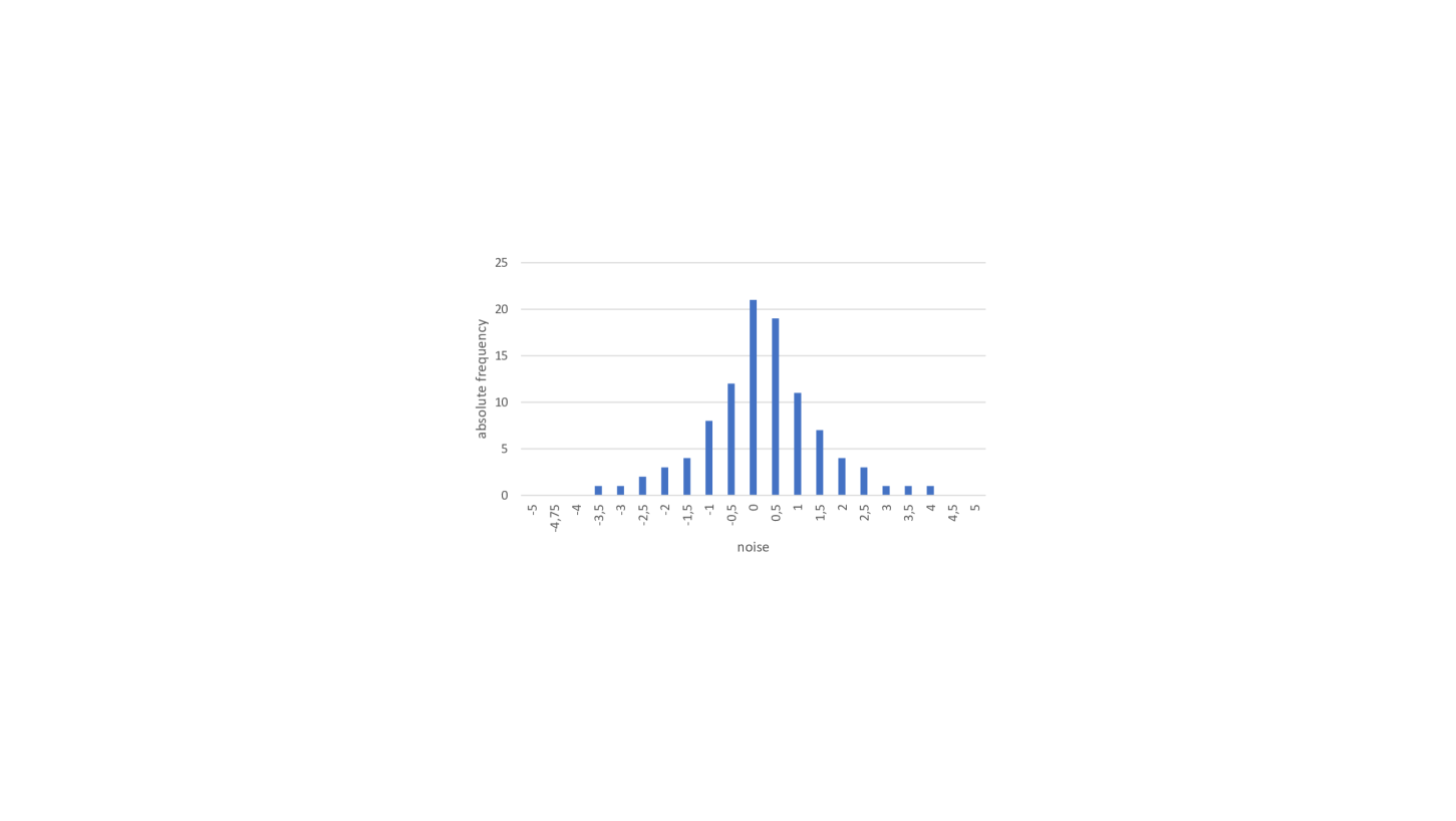
(a) Value of the noise depending on $p$.

(b) Histogram of the discretized Laplacian noise.

Figure 1: Derivation of the discretized Laplacian noise.

Now the clients are ready to generate their ZKPs that allows for verifying the validity of the clients’ local computations of $w^{\prime}$. Given the proposed architecture, the ZKP $\pi^{w}(a,b)$ with statement $a$ and witness $b$ that proves that $u$ has truthfully calculated $w^{\prime}$ has the following characteristic:

$$\pi^{w}\left(\left(w^{\prime},rt^{\mathbf{D}},\varepsilon_{\mu},\varepsilon_{\sigma},\varepsilon_{w^{\prime}},\varepsilon_{\mathrm{inverse}},\vartheta_{\mathbf{X}^{\intercal}Y},\vartheta_{\mathbf{Z}}\right),\left(\mathbf{D},\mathbf{Z}\right)\right).$$ (22)

Besides the above-described range proofs and computation checks, $\pi^{w}$ ensures a globally set range $\varepsilon_{w^{\prime}}$ for the submitted $w^{\prime}$:

$$\lVert w^{\prime}-\tilde{w}^{\prime}\rVert\leq\varepsilon_{w^{\prime}}.$$

Please refer to Section 3.2 for a detailed description of how we implement $\pi^{w}$.

Using a smart contract and through snarkjs’ export solidityverifier command, clients can, subsequently to compiling the circuit and generating the proof, upload their $w^{\prime}$ to the EVM. The smart contract verifies the proof and, if valid, uploads the client’s $w^{\prime}$.

3.1.2 Model Aggregation

For every successfully uploaded $w^{\prime}_{i}$, the smart contract Clients updates $w_{\mathrm{g}}$ by aggregating all weights that have been submitted to the smart contract so far using FedAvg. For a globally constant sample size $n$ in a LR setting, the respective aggregation formula equals

$$\begin{split}w_{\mathrm{g}}=\frac{\sum_{i=1}^{\lvert I\rvert}w_{i}}{\lvert I\rvert}\approx\frac{\sum_{i=1}^{\lvert I\rvert}w^{\prime}_{i}}{\lvert I\rvert}=w^{\prime}_{\mathrm{g}}\text{,}\end{split}$$ (23)

depending on $\epsilon$ and $\lvert I\rvert$. Heuristically, the noise is i.i.d. with expectation value $0$ and finite variance $2\lambda^{2}$, so by the law of large numbers, the probability that $w_{\mathrm{g}}$ differs significantly from $w^{\prime}_{\mathrm{g}}$ is small (in fact, the deviation is approximately normally distributed with standard deviation $\tfrac{2\lambda^{2}}{\sqrt{|I|}}$.

3.1.3 Compute and Prove Model Cost

After submitting and proving their LDP-weights $w^{\prime}$, clients test their unperturbed $w$ on a global and public data set $\mathbf{D}_{\textrm{test}}=(\mathbf{X}_{\mathrm{test}}~{}Y_{\mathrm{test}})=(X_{\mathrm{test},0}~{}X_{\mathrm{test},1}~{}\ldots~{}X_{\mathrm{test},k}~{}Y_{\mathrm{test}})\in\mathbb{R}^{n_{\mathrm{test}}\times(k+2)}$ with $X_{\mathrm{test}}=(1,...,1)^{\intercal}$, distributed via a public channel (e.g., a cloud provider). Clients have to prove that they computed their model cost $c$ truthfully based on $\mathbf{D}_{\textrm{test}}$ and using their $w$ by constructing a ZKP $\pi^{c}$ with the following characteristic.

$$\pi^{c}\left(\left(c,rt^{\mathbf{D}},rt^{\mathbf{D}_{\mathrm{test}}},\varepsilon_{w}\right),\left(\mathbf{D},\mathbf{Z},w\right)\right).$$ (24)

$\pi^{c}$ ensures that clients used the private input $w$ (i.e., their true and unperturbed weight) to compute $c$ by first reproducing $\tilde{w}$ in a circuit of the ZKP and performing the range proof (recall (12))

$$\lVert w-\tilde{w}\rVert\leq\varepsilon_{w}\quad\text{.}$$

Note that the SC Clients requires that clients have uploaded a valid $w$ prior to submitting and proving $c$, such that the standardization of $rt^{\mathbf{D}}$ as well as the effects of approximating $\lVert\mathbf{X}^{\intercal}Y\rVert$ through $\lVert\mathbf{Z}\rVert$ are already controlled by $\pi^{w}$. Then, as $w$ is a private input to $\pi^{c}$, we can compute $\tilde{c}$ in a circuit of $\pi^{c}$ and make sure that

$$\tilde{c}=\big{(}Y_{\mathrm{test}}-\hat{Y}_{\mathrm{test}}\big{)}^{\intercal}\big{(}Y_{\mathrm{test}}-\hat{Y}_{\mathrm{test}}\big{)}=c$$ (25)

with $\hat{Y}_{\mathrm{test}}=\mathbf{X}_{\mathrm{test}}\,\cdot\,w$ holds.

Second, by including $rt^{\mathbf{D}_{\mathrm{test}}}$ as a statement, $\pi^{c}$ can compute the respective Merkle tree on the test data set $\mathbf{D}^{\mathrm{test}}$ and require that the resulting root $\tilde{rt}^{\mathbf{D}_{\mathrm{test}}}$ equals $rt^{\mathbf{D}_{\mathrm{test}}}$, with the latter being stored in the EVM. Since $\mathbf{D}_{\mathrm{test}}$ is publicly available, all clients can easily check its standardization, such that checking $\tilde{rt}^{\mathbf{D}_{\mathrm{test}}}=rt^{\mathbf{D}_{\mathrm{test}}}$ is sufficient. This approach allows the system to guarantee truthful submissions of $c$ without having to store $\mathbf{D}_{\mathrm{test}}$ onchain, which would, depending on $k$ and $n_{\mathrm{test}}$ be costly and challenging. A detailed implementation of $\pi^{c}$ is again included in Section 3.2.

3.1.4 Compute Incentives

To translate $C=(c_{1},\dots,c_{|I|})^{\intercal}$ transparently into each client’s incentive payment $v_{i}$, we choose an efficient approach that can be computed on-chain by the Clients smart contract. First, we normalize all submitted and validated $c_{i}$’s to a vector $C_{\mathrm{norm}}\in\mathbb{R}^{|I|}$ that has expectation value $\mu=0$ and the standard deviation $\sigma=1$. We multiply all entries in $C_{\mathrm{norm}}$ with $(-1)$ as lower $c_{i}$ implies higher model performance and, subsequently, replace negative entries with $0$ (i.e., ensure that all $c_{\mathrm{norm,}i}$ that are higher than the mean of all $c_{i}$ are not incentivized). Next, we scale the data such that $\sum\limits_{i=0}^{|I|}c_{\mathrm{norm},i}=1$. Upon entry, clients have to pay an admission fee $B$, such that we can distribute the incentive payments $V=(v_{1},\dots,v_{|I|})^{\intercal}\in\mathbb{R}^{+}$ as follows:

$$V=B\cdot|I_{\mathrm{valid}}|\cdot C_{\mathrm{norm}}$$ (26)

where $|I_{\mathrm{valid}}|$ is the number of clients with valid $w^{\prime}_{i}$ and $c_{i}$. The payments are distributed by the function reward_clients() which can only be executed by the client who has initially deployed the Clients smart contract. Moreover, by using Solidity’s mapping, every client (i.e., address) can only register once as the data would be overwritten when joining multiple times and a new clientID would be set. We summarize the system outlined above in Table 2.

Step	Client $u_{i}$	Smart Contract
Training phase
1	Join system: Join the system by fetching the model $M_{i}$ (i.e., number of features $k$ and the sample size $n$), hashing $u_{i}$’s database, writing $rt^{\mathbf{D}}_{i}$ into storage, and paying the admission fee $B$
2	Train model: Train $M_{i}$ by computing $w_{i}$
3	Compute and upload LDP weight $w^{\prime}_{i}$: Compute and upload differentially private (LDP) weight $w^{\prime}_{i}$
4	Compute and submit weight proof $\pi^{w}_{i}$: Gen$\left(\pi^{w}_{i}\right)\rightarrow\pi^{w}_{i}$ and upload $\pi^{w}_{i}$. $w^{\prime}_{i}$ will only be uploaded into storage if $\pi^{w}_{i}$ is valid
5		Verify all LDP weights: Ver$\left(\pi^{w}_{i}\right)~{}\forall~{}i\in\{1,\ldots,\lvert I\rvert\}$. Write every $w^{\prime}_{i}$ into storage if $\pi^{w}_{i}$ has been validated
Testing phase
6		Global model aggregation: Aggregate all $w^{\prime}_{i}$ to $w^{\prime}_{\mathrm{g}}\approx w_{\mathrm{g}}$ and write $w^{\prime}_{\mathrm{g}}$ into storage
7	Compute $u_{i}$’s cost $\mathrm{c}_{i}$: Fetch the public test data set and evaluate own model performance (RSS) using $u_{i}$’s true weight $w_{i}$. Submit own accuracy as $u_{i}$’s cost $c_{i}$
8	Compute and upload cost proof $\pi^{c}_{i}$: Gen$\left(\pi^{c}_{i}\right)\rightarrow\pi^{c}_{i}$ and upload $\pi^{c}_{i}$. $c_{i}$ will only be uploaded into storage if $\pi^{c}_{i}$ is valid
9		Verify all cost proofs: Ver$\left(\pi^{c}_{i}\right)~{}\forall~{}i\in\{1,\ldots,\lvert I\rvert\}$
10		Compute incentives: Compute and distribute incentive payments $V$ according to $C$

Table 2: Steps of our protocol for private, fair, and honest FL.

3.2 Implementation

In this section, we describe the implementation of our architecture. Please note that, following circom terminology and in contrast to Section 3.1, we will now refer to single ‘circuits’ that are callable with input and output signals as ‘templates’, whereas we refer to a set of ‘templates’ that make up a ZKP as ‘circuits’. ‘Signals’ (signal) are the basis for defining constraints (using ===) and can only be assigned a value once (using <-- or -->). Both <== and ==> declare a constraint and assign a signal’s value at the same time. On the other hand, circom also includes conventional variables (var). As we use snarkjs and hence a framework for proof creation and verification based on SNARKs, a so-called trusted setup is required initially. It consists of two phases, one of which is independent of the circuit (‘powers of tau’) and that we could just import, as well as one that is circuit-specific. For implementation purposes, we conducted the trusted setup alone. However, for practical applications, a group of trusted parties would need to conduct an MPC such that the participants in the FL system would be confident that at least one group member deleted their input to the MPC.

We will include several, truncated source code excerpts throughout the following section. Please find the whole project on GitHub. Note that some templates are taken from iden3’s circomlib.

3.2.1 Weight Proof $\pi^{w}$

We start by explaining the implementation of $\pi^{w}$’s circuit, namely LinRegParams(...). First, we define the private and public inputs according to (24). The main template execution requires various variables (cf. listing 1), some of which are also input signals to the circuit for circom-specific reasons. Providing an untruthful value for some of these variables might make adversarial attacks possible. To make sure that these critical input variables are correct, the circuit requires the respective values as input signals to check equality. Listing 2 provides an overview of the implementation of $\pi^{w}$. The circuit as the basis for the ZKP is structured into five parts:

• Step 1 – Range proofs for $\varepsilon_{\mu}$ and $\varepsilon_{\sigma}$:
  To ensure that $\mathbf{D}$’s mean $\mu\approx 0$ and variance $\sigma\approx 1$, a certain accuracy is set by $\varepsilon_{\mu}$ and $\varepsilon_{\sigma}$ respectively. Based on both values, LinRegParams checks the accuracy of all $\mu$ and $\sigma$ for $X_{1},\ldots,X_{k}$ and $Y$. For example, setting in_require_meanxn_acc $=3$ would require that the absolute value of every $\mu\>\cdot\>n$ is smaller than $\varepsilon_{\mu}=10^{-3}$ (taking into account the conversion in (8) using $d$). Analogously, in_require_varxn sets the upper bound for $\sigma\>\cdot\>n$ via $\varepsilon_{\sigma}$.

• Step 2 – Check $rt^{\mathbf{D}}$:
  This step rebuilds $\mathbf{D}$’s Merkle tree with one data point (a prime field element as matrix entry) at each leaf. To improve the system’s performance, we do not hash the particular leaves on the lowest level since hashing is costly. This works because the hashing algorithm operates on big numbers that can be sufficiently large to cover any prime field element. After computing the tree, the template ensures that the computed root equals the public input $rt^{\mathbf{D}}$, which will be compared to the commitment specified at registration when calling the smart contract’s method Clients.

• Steps 3 and 6 – Range proofs for $\varepsilon_{\mathrm{inverse}}$ and $\varepsilon_{w^{\prime}}$:
  To verify the upper bound on $\varepsilon_{\mathrm{inverse}}$, the template checks the proximity of every entry in $\left((\mathbf{X}^{\intercal}\mathbf{X})\mathbf{Z}-\mathbbm{1}\right)$ to $0$. For example, setting in_require_XX_acc $=3$ would require that the absolute value of every entry is smaller than $\varepsilon_{\mathrm{inverse}}=10^{-3}$ (again taking into account the conversion in (8) using $d$). The same applies to in_require_b_noisy_acc, $\varepsilon_{w^{\prime}}$, and $w^{\prime}-\tilde{w}^{\prime}$.

• Steps 4 and 5 – Range proofs for $\vartheta_{\mathbf{Z}}$ and $\vartheta_{\mathbf{X}^{\intercal}Y}$
  Both $\vartheta_{\mathbf{Z}}$ and $\vartheta_{\mathbf{X}^{\intercal}Y}$ must be provided as inputs to the template in absolute numbers. The main template first finds the largest (by absolute value) entry in the matrix or vector using the maximum norm:

  $$\lVert\mathbf{A}\rVert=k\cdot\max\limits_{s,t}|a_{s,t}|$$ (27)

  where $\mathbf{A}$ can be either $\mathbf{Z}\in\mathbb{N}^{\left(k+1\right)\times\left(k+1\right)}$ or $\mathbf{\mathbf{X}^{\intercal}Y}\in\mathbb{N}^{k+1}$. Then it checks whether $0\leq\lVert\mathbf{A}\rVert\leq\vartheta_{\mathbf{A}}$ holds for both choices of $\mathbf{A}$.

Note that along with these six steps, the template performs the computation of $w^{\prime}$ iteratively. The LDP noise is added in the last step by generating $h_{j}$ using (20), choosing the respective LDP noise $q$ from $L$ using (19) and (21), as well as adding $q$ as in (17).

3.2.2 Cost Proof $\pi^{c}$

Next, we outline the implementation of $\pi^{c}$ in our proposed system, for which LinRegCost(...) is the main template. $\pi^{c}$’s private inputs (cf. lines 3 to 10 in Listing 3) resemble those of $\pi^{w}$ except for $w^{+}$ and $\mathrm{Sign}(w_{i})$, which are required to reproduce $c$ as outlined in Section 3.1.3. Note that the inputs of $\mathbf{D}_{\mathrm{test}}$ in lines 12 to 15 of Figure 3 are declared as private signals due to performance reasons (cf. Section 4 for details), even though they are publicly available. Also $\pi^{c}$ consists of five major steps to make sure that clients compute and submit their cost $c$ truthfully (cf. Listing 4):

• Steps 1 and 2 – Check $rt^{\mathbf{D}}$ and $rt^{\mathbf{D}_{\mathrm{test}}}$:
  In addition to checking the Merkle tree root $rt^{\mathbf{D}}$ (as in LinRegProof(...)), $\pi^{c}$ also ensures that clients calculate their $c$ based on the test data set $\mathbf{D}_{\mathrm{test}}=\left(\mathbf{X}_{\mathrm{test}}~{}Y_{\mathrm{test}}\right)$ by requiring $\tilde{rt}^{\mathbf{D}_{\mathrm{test}}}=rt^{\mathbf{D}_{\mathrm{test}}}$. $\mathbf{D}_{\mathrm{test}}$ is a standardized, publicly available, and central data set that is made available to all clients through a cloud service. Besides, $\mathbf{D}$’s standardization does not need to be checked again, as $\pi^{w}$ already ensures its standardization and $\pi^{c}$ verifies that $\tilde{rt}^{\mathbf{D}}$ equals $rt^{\mathbf{D}}$.

• Step 3 – Range proof for $\varepsilon_{w}$:
  Similar to step 5 in LinRegProof(...), we allow controlling $\lVert w-\tilde{w}\rVert$ by performing a range proof using the input $\varepsilon_{w}$. This means that essentially, the computation of the unperturbed weight $\tilde{w}$ is repeated and, subsequently, its proximity to $w$ is checked analogous to $\pi^{w}$’s range proof for $\varepsilon_{w^{\prime}}$.

• Steps 4 and 5 – Check $c$:
  First, as in (25), step 4 estimates $\hat{Y}_{\mathrm{test}}$. Second, step 5 derives $\tilde{c}$ and ensures that $\tilde{c}$ equals the submitted $c$.

3.2.3 Smart Contract

After introducing LinRegProof(...) and LinRegCost(...), this section provides an overview of the governance structure implied by the main smart contract, namely Clients. To reduce Clients’s size, we implemented lib as a support library. lib defines all structs required by Clients (cf. Listing 5) and repeatedly used methods like, e.g., proof verification calls. We will briefly introduce both major structs FL_client and FL_generic:

• FL_generic: Contains all global variables for, e.g., defining $k$, $n$, $rt^{\mathbf{D}_{\mathrm{test}}}$, $L$, or the variables to control the range proofs. The client that initially deploys the Clients smart contract must instantiate fl_generic, which will be the only global instance of the struct.

• FL_client: Upon registering, all clients are assigned to an instance fl_client (implemented via a mapping mapclient from the particular client’s address to the respective instance fl_client). FL_client includes all client-specific data as, for example, $w^{\prime}_{i}$, $rt^{\mathbf{D}}_{i}$, and both proofs.

To register, clients call the smart contract’s registerClient(...) function. As depicted in Listing 6, calling registerClient(...) requires $rt^{\mathbf{D}}_{i}$ as input, since clients must commit to their data set $\mathbf{D}_{i}$ upon joining the system. Further, they have to pay the admission fee $B$ defined in fl_generic which will be used to distribute the incentive payments later. Moreover, a clientID, a mapping mapID to connect the clients’ addresses with their clientID, and the current block hash (at the time of registering) serving as source of public randomness for deriving their LDP noise $p$ will be set automatically.

Subsequently, clients can upload their $w^{\prime}_{i}$ by calling the function uploadBeta(...) and delivering the following inputs:

• t_betaverifier: Address of the deployed weight verifier contract. The client must deploy this contract before calling uploadBeta(...) and provide the respective address such that other clients and uploadBeta(...) itself can verify the client’s weight proof.

• betaproof: This struct (cf. Listing 5) contains the actual proof, which is also the first part of the call data for verifying the weight proof.

• beta_noisy_true is the struct containing the submitted $w^{\prime}_{i}$.

uploadBeta(...) will collect the respective public inputs (cf. Listing 1) and, together with the provided betaproof, verify the proof $\pi^{w}$ onchain. Successfully verifying the proof requires correct input data $\mathrm{D}_{i}$, the correct approximate inverse $\mathrm{Z}$ (accuracy controlled by $d$), and correct computation of $w^{\prime}_{i}$. If successful, uploadBeta(...) saves the submitted beta (i.e., the client’s $w^{\prime}_{i}$), sets the client’s betaproof_valid to true, and updates betaglobal (i.e., $w_{g}$). The procedure is analogous (except for updating betaglobal) when submitting the cost $c_{i}$ by calling uploadCost(...), such that we will not further describe the function.

Eventually, to trigger the distribution of incentive payments, only the initial client t_initialclient can call the function Incentivize_clients(...). Incentivize_clients(...) will calculate the incentive payments $V$ and distribute them to those clients, who have successfully submitted their $w^{\prime}_{i}$, according to their contribution as described in Section 3.1.4. However, as this requires trust in the initial client (as only she/he can prompt the incentive payment by calling Incentivize_clients(...)), this way of triggering the payoff is probably not suitable in all scenarios. To make the trigger more trustless, the initial client could also specify ways to prompt the payoff. For example, any client could trigger it as soon as a certain threshold of participants is reached, or a certain amount of time (measured in the block number) has passed.

4 Evaluation

To evaluate our system, we ran several tests with different parameters. $k$ and $n$ are mainly influencing the complexity of our system, since they determine the number of Merkle tree leaves and, thus, the number of hashes that we compute in a SNARK. Note that more specifically, $(k+1)\,\cdot\,n$ for $\pi^{w}$ and $(k+1)\,\cdot\,(n+n_{\mathrm{test}})$ for $\pi^{c}$ determines the number of leaves since we leave out $X_{0,i}=(1,\ldots,1)$ and instead only hash $X_{1,i},\ldots,X_{k,i}$ as well as $Y_{i}$. Besides the number of leaves, also the choice of the hashing function can have a significant impact on the system performance. For example, when switching from ‘Poseidon’ [72] to ‘MiMC’ [73] hashing, the number of constraints of our system roughly increases by a factor $4$. Since this factor remains approximately the same when increasing circuit complexity (i.e., the number of constraints), we tested our artifact only with ‘Poseidon’ hashes on an AWS instance (Ubuntu 20.04, 16 virtual CPU cores, and 64 GB RAM). Instead of snarkjs’ default web assembly compiler, we used a native compiler (C++) that can handle larger circuits.

Table 3 provides an excerpt of our test results (Tables 4 and 5 in the appendix contain the entire test data for $\pi^{w}$ and $\pi^{c}$ respectively). Note that we used rapidsnark to generate the proofs (cf. “proof gen duration”). Besides, due to their similar implementation (cf. Section 3.2), the cost proof’s performance test results do not differ significantly from the weight proof’s results. We will, therefore, mainly focus on the weight proof’s results:

$k$	$n$	$(k+1)\,\cdot\,n$	# constraints	key gen duration (s)	proof gen duration (s)	verification duration (s)	circuit size (MB)	verification key size (kB)	proof size (bytes)
4	100	500	89,819	177	8.641	0.236	46	25	708
4	250	1,250	208,162	337	19.410	0.237	102	25	709
4	500	2,500	404,962	659	36.868	0.237	198	25	708
4	750	3,750	601,520	1089	57.042	0.237	310	25	705
4	1,000	5,000	798,659	1360	74.945	0.232	391	25	705
4	1,500	7,500	1,190,620	2571	120.736	0.263	614	25	705

Table 3: Evaluation of essential parameters for building and verifying the $\pi^{w}$ circuit depending on $k$ and $n$.

Before analyzing our system’s performance, we describe an essential optimization that prior tests suggested: We found that the recomputations of the Merkle trees are the artifact’s dominating operations in terms of constraints. Therefore, we optimized the computation of $rt^{\mathbf{D}}$ and $rt^{\mathbf{D}_{\mathrm{test}}}$ by hashing six instead of two data points at the leaf level at once and hard-coding ‘empty’ leaf hashes to avoid additional hashing in those Merkle trees that are not entirely filled with data points on the leaf level (depending on $k$, $n$, and $n_{\mathrm{test}}$, not every leaf necessarily represents a data point as the bottom level must – given our Merkle tree optimization – always contain $2^{\,\mathrm{depth}}\,\cdot\,3$ leaves). This optimization reduced the circuit complexity by roughly 50%. Then, computing the circuit-specific trusted setup for a LR on a training data set with $k=4$ features and sample size $n=1,000$ per client in a FL setting takes roughly $23$ minutes each for $\pi^{w}$ (cf. Table 3) and $\pi^{c}$ (cf. Table 5 in the appendix). Note that, as outlined above, the circuit-specific trusted setup must only be computed once and can then be used by all clients for a particular FL learning task. Using the proving key from the trusted setup, every client must spend roughly $2.5$ minutes on computing both proofs that allow fellow clients to verify their submitted weight $w$ and cost $c$ (for $k=4$ and $n=1,000$). In practical FL applications, the proof generation likely runs on less sophisticated machines than our AWS instance. We, therefore, also tested the proof duration on a single CPU core (also for combinations other than $k=4$ and $n=1,000$). The results reveal that the witness generation duration was not sensitive to this limitation, whereas the duration for generating the proof using rapidsnark increased seven times from $4.3$ to $29.4$ seconds and the proof verification duration four times from $0.24$ to $0.97$ seconds. In total, the proof duration grew $1.4$ times from around $75$ to $103$ seconds. Moreover, the RAM required to generate and validate proofs remains below 4 GB and agnostic to the number of constraints. Looking at the performance of the system’s smart contract on the EVM, we find gas cost of around $2.2$ million for all $\pi^{w}$-related on-chain operations and $920,000$ for all $\pi^{c}$-related operations. This translates into a total of roughly USD $1270$ for all on-chain operations (USD $900$ for $\pi^{w}$ operations and USD $370$ for $\pi^{c}$ operations) per client, given a gas price of 100 gwei and a rate of 1 ETH = USD 4,000. While in absolute terms this is prohibitively expensive, it is only $21\%$ of the current public Ethereum target block capacity as well as $10.5\%$ of the block limit. Note that the $\pi^{c}$ operations are significantly cheaper than the $\pi^{w}$ operations, mainly since the latter requires the vector $L$ as public input and updates $w_{\mathrm{g}}$. As long as operations on public blockchains are that costly, using a permissioned blockchain like Quorum can allow not only to reduce costs but also allowing for considerably higher throughput [74].

To assess our system’s scalability, we focus on analyzing the impacts of increasing $k$, $n$, and $n_{\mathrm{test}}$ on the circuit-specific trusted setup, the proof generation and verification, as well as the gas cost of the smart contract. Both Figure 2 and Table 3 show results that are in line with the expected scaling properties of SNARKs: The computation of the circuit-specific trusted setups (i.e., ‘key gen duration’) as well as the time it takes to generate the proofs (i.e., ‘proof duration’) scale linearly with $(k+1)\,\cdot\,n$ or $(k+1)\,\cdot\,(n+n_{\mathrm{test}})$ (cf. Table 5 in the appendix). Moreover, verification duration, verification key size, and proof size do not significantly change when increasing the circuit complexity. Thus, increasing $k$, $n$, or $n_{\mathrm{test}}$ will have only minor effects on the system’s overall computation effort, since the proof duration might grow for an individual client whilst the redundant on-chain proof storage and verification cost will remain constant. Even when translating our results to circuits as huge as those in the Hermez project (the project also used circom with snarkjs and manages to compute a proof for around $100$ million constraints in few minutes on a server with 64 virtual cores and 1 TB RAM [75]), we find promising scaling performance: Given the test results, we expect that $\pi^{w}$ and $\pi^{c}$ with $(k+1)\,\cdot\,n=600,000$ data points and $n_{\mathrm{test}}=0.1\,\cdot\,n=6,000$ would result in roughly $100$ million constraints and hence be feasible to prove in a few minutes to hours per proof (depending on the hardware used; in our setup roughly $2.5$ hours with 16 CPU cores or approximately $3.5$ hours with one core) whilst handling a huge sample size (e.g., $k=5$ and $n=100,000$). In this case, the one-time trusted setups would take a few hours to a few days for each participant of the trusted setup (which we assume will not necessarily be conducted by the clients in practice, but a small to medium-sized group or maybe also research institutions, as could be observed for the trusted setup used in Z-Cash, zkSync, etc.). Besides, we expect the verification duration, verification key size, and proof size to remain constant in this scenario.

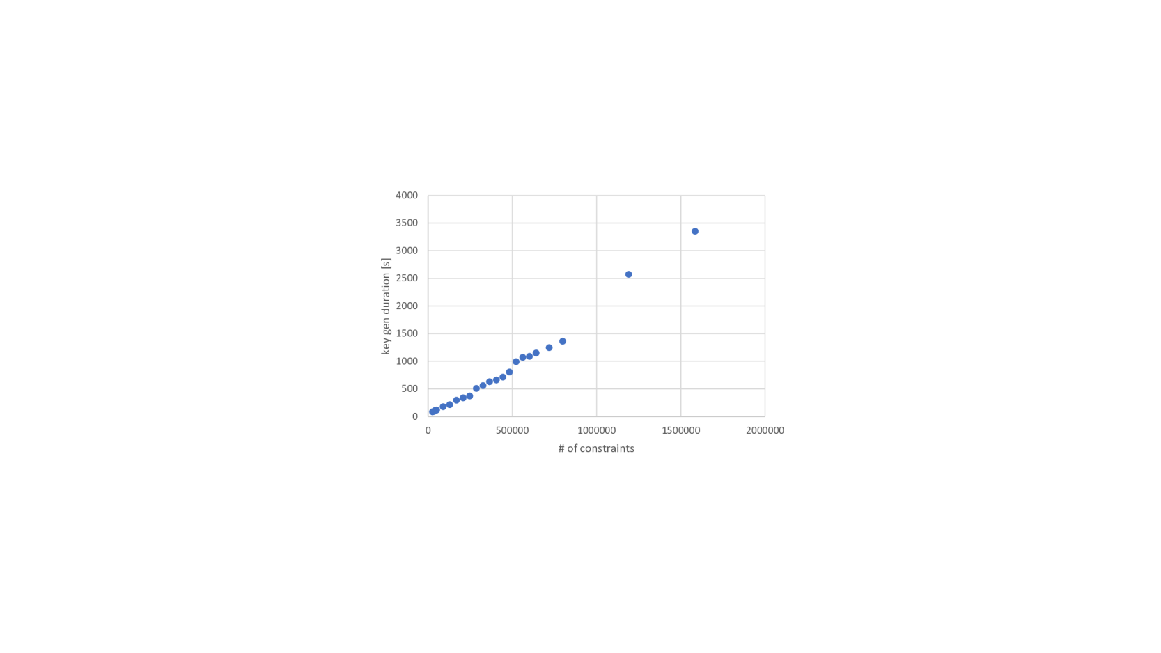
(a) Scaling of the circuit complexity (i.e., the number of constraints) with $(k+1)\,\cdot\,n$.

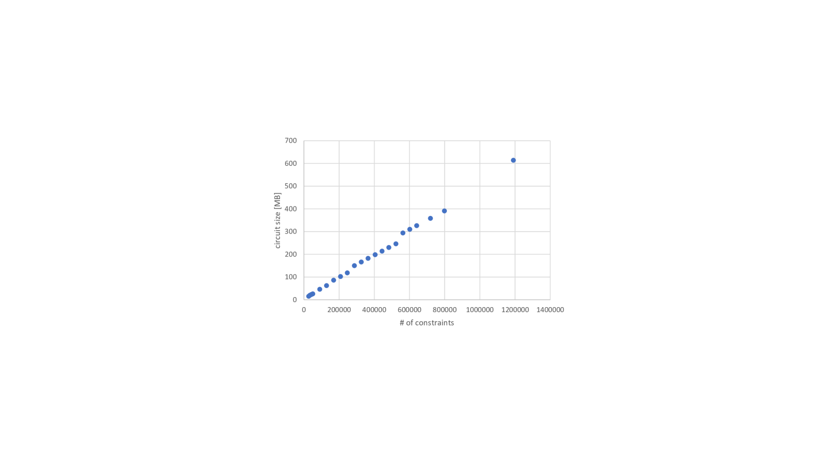
(b) Scaling of the verification duration, verification key size, and proof size with the number of constraints.

Figure 2: $\pi^{w}$ scalability analysis (client perspective).

Also, the gas cost for the EVM operations is independent of the proof complexity. The only data that must be stored on-chain to verify a proof are the proof itself, the verification key, and the public inputs. Both the proof size as well as the verification key size are constant for every $k$, $n$, and $n_{\mathrm{test}}$. The public inputs’ volume only increases when either the number of features $k$ or the LDP noise discretization interval $d_{\mathcal{L}}$ grows, since this leads to an increase in the number of entries in the weight vector $w^{\prime}$ or the LDP noise vector $L$. Thus, raising $w^{\prime}$ or $L$ increases the payload size, which in turn leads to a rise in gas cost. However, for moderate $k$ and $d_{\mathcal{L}}$, the total gas cost remains small since the respective proof verification itself is responsible for the major part of the gas cost. Therefore, both proofs can be stored as well as verified cheaply on-chain also for large circuits and the particular gas cost remains, as mentioned above, approximately at $2.2$ million for all $\pi^{w}$-related on-chain operations and $920,000$ for all $\pi^{c}$-related operations. Eventually, a clients’ effort does not grow with the size of other clients’ underlying data sets or the number of participating clients. Further, the number of on-chain transactions only grows linearly with the number of clients and is independent of the size of the clients’ training data as well as the central test data. These results promise high potential also for more sophisticated ML applications that require higher data volumes.

Eventually, we refrain from testing the accuracy of our FL system. The only difference regarding accuracy between our and a plain FL system is the LDP noise that we add to the clients’ weights; and since aggregation is an average over all local weights plus noise, this difference is just an average of i.i.d. Laplacian-distributed random variables, which has mean $0$ and standard deviation proportional to $\frac{\varepsilon}{\sqrt{\lvert I\rvert}}$. The value of $\varepsilon$ and $\lvert I\rvert$ hence completely determine the change in accuracy of our approach compared to the literature.

5 Discussion and Conclusion

Our paper aims at answering the research question of how a FL system can achieve fairness, integrity, and privacy simultaneously whilst still being practical and scalable. After identifying a business need for these requirements and arguing that related work so far has not proposed an architecture that satisfies them, we described our proposed system in Section 3 based on a combination of blockchain, ZKP, and LDP. Our conceptual discussion of the architecture and the experiments that we describe in Section 4 suggest that our implementation indeed offers a practical solution to confidential, fair, and tamper-resistant FL that achieves reasonable performance and scalability properties for LRs. Next to suggesting a pathway to effectively combining FL with blockchain, ZKP, and LDP, we develop a system that allows clients to verifying that other clients truthfully trained their local model and received a fair compensation for participating in the case of LR. Thus, we go beyond existing research that has suggested ZKPs for verifying ML model inference based on already trained models.

However, our research is not without limitations and reveals potential for future research that we will outline in this section to conclude our paper. First, even though our suggested system does currently only support LRs, we tried to design it as generic as possible to allow for adapting the system to other classes of ML protocols. Specifically, we move computationally intensive parts (in our case, the inversion of $\mathbf{X}^{\intercal}\mathbf{X}$) outside the circuit and only check certain properties of the result (in our case, that the approximate inverse that must be provided as private input to the ZKP is indeed close to the true inverse, cf. Section 3.1.1) rather than recomputing the result. For the case of LR, we derived an error bound (see (16)) that allowed us to significantly reduce the complexity of the respective circuit while maintaining full tamper resistance. The approach of only proving specific properties that the local weights need to satisfy to indicate the integrity of training may be generalizable to further classes of ML models, also considering the recent advancement in using ZKPs for frequent operations in ML (e.g., [65]). Since training ML models often involves solving a convex optimization problem where optimality can be checked locally (e.g., all partial derivatives in the allowed directions are $0$) [76], we encourage future research to adapt the suggested architecture to more sophisticated classes of ML models beyond LR. Furthermore, the aggregation of weights in federated learning is often linear [25], so our concept of perturbing the local weights with verifiable noise is applicable beyond multiple LRs: Assuming that the training data is i.i.d. (a common assumption in FL applications), the local weights are also i.i.d.. Moreover, as we construct the clients’ LDP noise from a random oracle, the noise is also i.i.d. and has mean $0$ and finite variance by construction. Since the weights and the noise applied to them are by construction independent, by the linearity of the averaging algorithm FedAvg, the error in the global model is a weighted average of local noise and the random variable (noise times weight) is i.i.d. with expectation value $0$ and finite variance. By the law of large numbers, the error in the aggregated global model hence converges to $0$. Thus, for a large number of clients, the error term in the aggregate model as introduced by LDP is typically small. It follows that our approach of using LDP (which has been proposed by several other scholars but is particularly relevant in our system because we can prove not only the correct training but also the correct addition of noise) extends to more sophisticated ML models beyond LR.

To further improve the performance and practicality of our system, we aim at implementing the ZKPs via STARKs for improved proof creation performance, post-quantum security, and eliminating the need for a trusted setup in the future. Further, the system’s scalability would further benefit from a recursive verification mechanism that reduces the complexity of verifying weight and cost proofs. This could be implemented by building on batching techniques [77] or recursive proofs [78, 79] and would facilitate scalability by hierarchical aggregation (e.g., only $\log(\lvert I\rvert)$ verification steps would be required on-chain). Besides, even though recalculating $w$ in $\pi^{c}$ is not the proof’s main complexity driver, we see optimization potential there: One could commit a hash of the weight (without noise) and some random salt in the smart contract (proving that the hash was computed like that), so for computing the costs we only need to prove that we used the pre-image of this hash (without salt) for the computation. This can further reduce the cost proof’s number of constraints. Next to optimizations of our own code and the performance improvements in libraries that support the generation of ZKP (e.g., STARKs or circom 2.0), we are also confident that hardware acceleration for faster ZKP-related operations and particularly proving will be available soon, as research in this area is already conducted, e.g., by projects that build on Ethereum and that leverage ZKPs [80]. This may allow getting even shorter proof times also on devices that are computationally more restricted than a Laptop.

Moreover, we acknowledge that there are still some attacks on integrity: When clients know the learning task (i.e., in our case, the parameters stored on fl_generic) prior to committing their data when joining the system, they could attack the system by manipulating their data set before committing to it. However, reverse engineering the data in order to get a desired (malicious) result for the weights is likely more effort than just contributing arbitrarily chosen weights. Moreover, we expect many use cases for our proposed system to be built on sensor data (e.g., from vehicular networks or health applications). Given this, and the availability of certified sensors (e.g., by means of a crypto-chip on the sensor and a certificate of the manufacturer), as are emerging, for example, in Germany’s Smart Meter rollout [81], the ZKP-based approach could handle this issue by including a proof of authenticity (i.e., a proof that the data was signed by a private key that is bound to a certificate that was in turn signed by a trusted, publicly known entity) for the sensor input data when committing to it. This would be easy to integrate at the costs of an additional signature verification per Merkle tree leaf (around 5,000 constraints per leaf for a Schnorr signature). This still does not protect against physical manipulation (imagine putting a temperature sensor to a place where it is not supposed to be), but may offer a reasonable degree of trust in data provenance in many practical scenarios.

Our current incentive mechanism relies on the existence of a central and public data set as described in Section 3.1.4. Since we acknowledge that this hypothesis is not always feasible in practice, we will work on developing other, effective incentive mechanisms. In doing so, we intend to ensure the mechanisms’ fairness by incorporating the research of Shapley [82]. In doing so, our construction allows us to perform the local evaluation of each client on their actual weights with and without noise, so we get new degrees of freedom for proving the correct evaluation and deriving fair incentives.

Lastly, to ensure the system’s applicability in practice, we plan a twofold approach. First, as we are currently training the test model on the California Housing Prices data set, we will also run accuracy tests to assess how our conceptual approach translates into data-related performance in practice. Second, we will evaluate the perspective of enterprises on the new features that the combination of FL with blockchain technology, LDP, and ZKP offers.

We believe that the convergence of emerging technologies like ML and blockchains in the context of data generated by the IoT, as Guggenberger et al. [83] or Singh et al. [84] suggest, combined with privacy-enhancing technologies in the context of sensor data sharing or derived models in data markets [51], has the potential to facilitate many new use cases as well as business models and can inspire the field of computer science. As all these aspects are relevant for FL, we are expecting interesting results that further extend our design to more complex models in the future.  
 
Acknowledgment: We want to thank Orestis Papageorgiou, who pointed us to the work of Newman [67], and Jordi Baylina and the iden3-Team for their great work on circom and snarkjs and their helpful responses to our questions. Moreover, we thank Matthias Babel, Jonas Berweiler, Dennis Jelito, and Michael Reichle for their ad-hoc problem-solving support. We also gratefully acknowledge the Bavarian Ministry of Economic Affairs, Regional Development and Energy for their funding of the project “Fraunhofer Blockchain Center (20-3066-2-6-14)” that made this paper possible.

Appendix

5.1 Selected Code Snippets

⬇

1template LinRegParams(k, n, dec, l_train, require_meanxn_acc, require_varxn_acc, require_XX_acc, require_XX_inv_maxnorm, require_X_trans_Y_maxnorm, require_b_noisy_acc, hash_alg, DP_acc) {

2

3 signal private input in_x_pos[k][n]; // $(\mathbf{X}_{i})^{+}$

4 signal private input in_x_sign[k][n]; // $\mathbf{Sign(X)}_{i}$

5 signal private input in_y_pos[n][1]; // $(Y_{i})^{+}$

6 signal private input in_y_sign[n][1]; // $\mathrm{Sign}(Y_{i})$

7 signal private input in_xx_inv_pos[k][k]; // $(\mathbf{Z}_{i})^{+}$

8 signal private input in_xx_inv_sign[k][k]; // $\mathbf{Sign(Z)}_{i}$

9 //public inputs:

10 signal input in_k; // $k$

11 signal input in_n; // $n$

12 signal input in_dec; // $d$

13 signal input in_merkleroot_train; // $rt^{\mathbf{D}}_{i}$

14 signal input in_Lap_X_pos[DP_acc - 1]; // $L$

15 signal input in_DP_acc; // $d_{\mathcal{L}}$

16 signal input in_hash_BC; // $\mathrm{block~{}hash~{}or~{}other~{}source~{}of~{}public~{}randomness}$

17 signal input in_b_noisy_true_pos[k][1]; // $(w^{\prime}_{i})^{+}$

18 signal input in_b_noisy_true_sign[k][1]; // $\mathrm{Sign}(w^{\prime})_{i}$

19 signal input in_require_meanxn_acc; // $\sim\varepsilon_{\mu}$

20 signal input in_require_varxn_acc; // $\sim\varepsilon_{\sigma}$

21 signal input in_require_XX_acc; // $\sim\varepsilon_{\mathrm{inverse}}$

22 signal input in_require_XX_inv_maxnorm; // $\vartheta_{\mathbf{Z}}$

23 signal input in_require_X_trans_Y_maxnorm; // $\vartheta_{\mathbf{X}^{\intercal}Y}$

24 signal input in_require_b_noisy_acc; // $\sim\varepsilon_{w^{\prime}}$

25

26 ...

Listing 1: Excerpt from the circuit for the weight proof $\pi^{w}$ – Input signals. The default visibility for inputs is public.

⬇

1 ...

2

3 // 1. step | Check data normalization (i.e., $\varepsilon_{\mu}\approx 0$ and $\varepsilon_{\sigma}\approx 1$)

4 component check_mean = Check_MeanXY(k, n, dec, require_meanxn_acc);

5 ...

6 //make sure that range_meanxn_acc.out is within the bound $\varepsilon_{\mu}$

7 component range_meanxn_acc = GreaterEqThan(...);

8 ...

9 1 === range_meanxn_acc.out;

10 ...

11 component check_var = Check_VarXY(k, n, dec, ..., require_varxn_acc);

12 ...

13 //make sure that range_varxn_acc.out is within the bound $\varepsilon_{\sigma}$

14 component range_varxn_acc = GreaterEqThan(bits_range_varxn_acc);

15 ...

16 1 === range_varxn_acc.out;

17

18

19 // 2. step | Check $rt^{\mathbf{D}}_{i}$

20 component merkleproof_train = MerkleProof_six(k, n, l_train, hash_alg);

21 ...

22 //make sure that $rt^{\mathbf{D}}_{i}$ is correct

23 in_merkleroot_train === merkleproof_train.out;

24 ...

25

26 // 3. step | range proof $\varepsilon_{\mathrm{inverse}}$

27 component XX_rangeproof = XX_RangeProof(k, n, require_XX_acc, dec);

28 ...

29 //make sure that range_XX_acc.out is within the bound $\varepsilon_{\mathrm{inverse}}$

30 component range_XX_acc = GreaterEqThan(...);

31 ...

32 1 === range_XX_acc.out;

33

34 // 4. step | range proof $\vartheta_{\mathbf{Z}}$

35 component maxelement_XX_inv_pos = NormMaxElement(k, k, ...);

36 ...

37 //make sure that $k\>\cdot\>range\_XX\_inv\_norm.out$ is within the bound $\vartheta_{\mathbf{Z}}$

38 component range_XX_inv_norm = LessEqThan(...);

39 1 === range_XX_inv_norm.out;

40

41 // 5. step | range proof $\vartheta_{\mathbf{X}^{\intercal}Y}$

42 //compute $\mathbf{X}_{i}^{\intercal}Y_{i}$

43 component X_trans_Y_mult = MatrixMult(n, k, 1);

44 ...

45 component maxelement_X_trans_Y_pos = VectorNormMaxElement(k, ...);

46 ...

47 //make sure that (\textcolor{gray}{$*k\:\cdot\:$maxelement\_X\_trans\_Y\_pos.out$ is within the bound $\vartheta_{\mathbf{X}^{\intercal} Y}$}*)

48 component range_X_trans_Y_norm = LessEqThan(...);

49 1 === range_X_trans_Y_norm.out;

50

51 // 6. step | range proof $\varepsilon_{w^{\prime}}$

52 component b_rangeproof_noisy = b_noisy_RangeProof(k, n, require_b_noisy_acc, hash_alg,

53 dec, DP_acc);

54 ...

55 //make sure that range_b_noisy_acc.out is within the bound $\varepsilon_{w^{\prime}}$

56 component range_b_noisy_acc = GreaterEqThan(require_b_noisy_acc);

57 1 === range_b_noisy_acc.out;

58}

59component main = LinRegParams(...);

Listing 2: Excerpt from the circuit for the weight proof $\pi^{w}$ – Main part.

⬇

1template LinRegCost(k, n, n_test, dec, l_train, l_test, hash_alg, require_b_acc) {

2

3 signal private input in_x_pos[k][n]; // $(\mathbf{X}_{i})^{+}$

4 signal private input in_x_sign[k][n]; // $\mathbf{Sign(X)}_{i}$

5 signal private input in_y_pos[n][1]; // $(Y_{i})^{+}$

6 signal private input in_y_sign[n][1]; // $\mathrm{Sign}(Y_{i})$

7 signal private input in_b_true_pos[k][1]; // $(w_{i})^{+}$

8 signal private input in_b_true_sign[k][1]; // $\mathrm{Sign}(w_{i})$

9 signal private input in_xx_inv_pos[k][k]; // $(\mathbf{Z}_{i})^{+}$

10 signal private input in_xx_inv_sign[k][k]; // $\mathbf{Sign(Z)}_{i}$

11 //$\mathbf{D}^{\mathrm{test}}$ is not set as public to reduce onchain data volume

12 signal private input in_x_test_pos[k][n_test]; // $(\mathbf{X}_{\mathrm{test}})^{+}$

13 signal private input in_x_test_sign[k][n_test]; // $\mathbf{Sign(X)}_{\mathrm{test}}$

14 signal private input in_y_test_pos[n_test][1]; // $(Y_{\mathrm{test}})^{+}$

15 signal private input in_y_test_sign[n_test][1]; // $\mathrm{Sign}(Y)_{\mathrm{test}}$

16 //public inputs:

17 signal input in_cost_submitted; // $c_{i}$

18 signal input in_k; // $k$

19 signal input in_n; // $n$

20 signal input in_n_test; // $n_{\mathrm{test}}$

21 signal input in_dec; // $d$

22 signal input in_merkleroot_train; // $rt^{\mathbf{D}}_{i}$

23 signal input in_merkleroot_test; // $rt^{\mathbf{D}_{\mathrm{test}}}$

24 signal input in_require_b_acc; // $\sim\varepsilon_{w}$

25

26 ...

Listing 3: Excerpt from the circuit for the cost proof $\pi^{c}$ – Input signals. The default visibility for inputs is public.

⬇

1 ...

2

3 // 1. step | Check $rt^{\mathbf{D}}_{i}$

4 component merkleproof_train = MerkleProof_six(k, n, l_train, hash_alg);

5 ...

6 //make sure that $rt^{\mathbf{D}}_{i}$ is correct

7 in_merkleroot_train === merkleproof_train.out;

8

9 // 2. step | Check $rt^{\mathbf{D}_{\mathrm{test}}}$

10 component merkleproof_test = MerkleProof_six(k, n_test, l_test, hash_alg);

11 ...

12 //make sure that $rt^{\mathbf{D}_{\mathrm{test}}}$ is correct

13 in_merkleroot_test === merkleproof_test.out;

14

15 // 3. step | range proof $w_{i}$

16 component b_rangeproof = b_RangeProof(k, n, require_b_acc, hash_alg, dec);

17 ...

18 //make sure that range_b_true_acc.out is within the bound $\varepsilon_{w}$

19 component range_b_true_acc = GreaterEqThan(...);

20 1 === range_b_true_acc.out;

21

22 // 4. step | compute $\hat{Y}_{\mathrm{test},i}$

23 //compute $\mathbf{X}^{\intercal}$

24 signal x_test_trans_pos[n_test][k];

25 signal x_test_trans_sign[n_test][k];

26 ...

27 //calculate $\hat{Y}_{\mathrm{test},i}$

28 component y_est_mult = MatrixMult(k, n_test, 1);

29 ...

30

31 // 5. step | compute $\tilde{c}_{i}$

32 ...

33 signal y_est[n_test];

34 signal y_test[n_test];

35 signal y_test_tmp[n_test];

36 component cost_sum = SigSum(n_test);

37 ...

38 //make sure that $c_{i}=\tilde{c}_{i}$

39 in_cost_submitted === cost_sum.out;

40}

Listing 4: Excerpt from the circuit for the cost proof $\pi^{c}$ – Main part.

⬇

1library lib {

2 ...

3 // beta

4 struct Beta {

5 uint[] beta_pos; // $(w^{\prime}_{i})^{+}$

6 uint8[] beta_sign; // $\mathrm{Sign}(w^{\prime})_{i}$

7 }

8 struct BetaGlobal {

9 Beta beta; // $w_{\mathrm{g}}$

10 uint16 I_round; // number of participants with valid $\pi^{w}_{i}$

11 }

12 struct Proof {

13 uint[2] a;

14 uint[2][2] b; // proof.json

15 uint[2] c;

16 }

17

18 // cost struct

19 struct FL_cost {

20 uint[] cost; // $C$

21 address payable[] t_cost;

22 }

23

24 // client struct

25 struct FL_client {

26 uint16 clientID;

27 uint merkleroot_train; // $rt^{\mathbf{D}_{i}}$

28 uint hash_BC; // current block hash

29

30 Beta beta_noisy_true; // $(w^{\prime}_{i})$

31 address t_betaverifier;

32 Proof betaproof;

33 bool betaproof_valid;

34

35 uint cost; // $c_{i}$

36 address t_costverifier;

37 Proof costproof;

38 }

39

40 // generic struct

41 struct FL_generic {

42 uint admission_fee; // $k$ in wei

43 uint8 k; // $k$

44 uint n; // $n$

45 uint n_test; // $n_{\mathrm{test}}$

46 uint8 dec; // $d$

47 uint DP_acc; // $d_{\mathcal{L}}$

48 uint merkleroot_test; // $rt^{\mathbf{D}_{\mathrm{test}}}$

49 uint[] Lap_X_pos; // $(L)^{+}$

50 uint8 require_meanxn_acc; // $\sim\varepsilon_{\mu}$

51 uint8 require_varxn_acc; // $\sim\varepsilon_{\sigma}$

52 uint8 require_XX_acc; // $\sim\varepsilon_{\mathrm{inverse}}$

53 uint require_XX_inv_maxnorm; // $\vartheta_{\mathbf{Z}}$

54 uint require_X_trans_Y_maxnorm; // $\vartheta_{\mathbf{X}^{\intercal}Y}$

55 uint8 require_b_noisy_acc; // $\sim\varepsilon_{w^{\prime}}$

56 uint8 require_b_acc; // $\sim\varepsilon_{w}$

57 uint8 hash_alg; // $hash\_alg$

58 }

59 ...

60}

Listing 5: Excerpt from the client smart contract – Support library.

⬇

1...

2contract Clients {

3

4 //generic variables

5 uint16 public count;

6 uint32 constant betaproof_publicinput_length = 119;

7 address public t_initialclient;

8 uint[] public incentives;

9

10

11 // initialize structs

12 lib.FL_generic fl_generic;

13 lib.BetaGlobal betaglobal;

14 lib.FL_cost fl_cost;

15

16 // mappings

17 mapping (address => lib.FL_client) public mapclient;

18 mapping (uint => address) public mapID;

19

20 constructor(lib.FL_generic memory _fl_generic) {

21 count = 0;

22 t_initialclient = msg.sender;

23 fl_generic = _fl_generic;

24 }

25

26

27 //

28 // functions

29 //

30

31 function registerClient(uint _merkleroot_train) public payable {

32 count++;

33 mapID[count] = msg.sender;

34 mapclient[msg.sender].clientID = count;

35 mapclient[msg.sender].merkleroot_train = _merkleroot_train;

36 mapclient[msg.sender].hash_BC = uint(blockhash(block.number));

37

38 // require that fee has been paid

39 require(msg.value >= fl_generic.admission_fee, "Pay fee");

40 }

41

42 function uploadBeta(lib.Proof memory _betaproof, lib.Beta memory _beta_noisy_true, address _t_betaverifier) public {

43 // upload proof

44 mapclient[msg.sender].t_betaverifier = _t_betaverifier; // address of deployed verifier SC

45 mapclient[msg.sender].betaproof = _betaproof;

46

47 // upload beta

48 mapclient[msg.sender].beta_noisy_true = _beta_noisy_true;

49

50 // verify beta proof

51 bool proof = lib.verifyBeta(fl_generic, mapclient[msg.sender]);

52 require (proof, "proof failed"); // no beta will be stored if proof fails

53 mapclient[msg.sender].betaproof_valid = proof;

54

55 // update betaglobal

56 lib.Beta[] memory beta_all_valid = new lib.Beta[](count);

57 uint16 i_valid = 0;

58 for (uint16 i = 1; i <= count; i++) {

59 if (mapclient[getClientAddress(i)].betaproof_valid) {

60 beta_all_valid[i_valid] = mapclient[getClientAddress(i)].beta_noisy_true;

61 i_valid++;

62 }

63 }

64 betaglobal = lib.genBetaMean(beta_all_valid);

65 }

66

67 function uploadCost(lib.Proof memory _costproof, uint _cost, address _t_costverifier) public {

68 // make sure that client contributed

69 require(mapclient[msg.sender].betaproof_valid, "no beta");

70

71 // upload proof

72 mapclient[msg.sender].t_costverifier = _t_costverifier; // address of deployed verifier SC

73 mapclient[msg.sender].costproof = _costproof;

74

75 // upload cost

76 mapclient[msg.sender].cost = _cost;

77

78 // verify cost proof

79 bool proof = lib.verifyCost(fl_generic, mapclient[msg.sender]);

80 require(proof, "proof failed"); // no cost will be stored if proof fails

81

82 // upload to fl_cost

83 fl_cost.cost.push(_cost);

84 fl_cost.t_cost.push(payable(msg.sender));

85 }

86

87 function Incentivize_clients () public payable {

88 // make sure that only initial client can trigger incentive distribution

89 require(msg.sender == t_initialclient, "only initclient");

90

91 // get incentives

92 incentives = lib.calcIncentives(fl_cost.cost, fl_generic.admission_fee);

93

94 // pay incentives

95 require(address(this).balance >= incentives.length * fl_generic.admission_fee, "low balance");

96 for (uint16 i = 0; i < count; i++) {

97 fl_cost.t_cost[i].transfer(incentives[i]);

98 }

99 }

100 ...

101}

Listing 6: Excerpt from the client smart contract – Main part.

5.2 Performance of the $\pi^{w}$ circuit

$k$	$n$	$(k+1)\,\cdot\,n$	# constraints	key gen duration (s)	proof gen duration (s)	verification duration (s)	circuit size (MB)	verification key size (kB)	proof size (bytes)
4	20	100	26,894	84	2.981	0.238	15	25	707
4	30	150	34,340	93	3.619	0.239	20	25	710
4	40	200	42,834	113	4.530	0.245	23	25	707
4	50	250	50,272	117	5.091	0.239	26	25	705
4	100	500	89,819	177	8.641	0.236	46	25	708
4	150	750	128,362	213	12.080	0.238	62	25	706
4	200	1,000	168,619	294	15.996	0.241	86	25	706
4	250	1,250	208,162	337	19.410	0.237	102	25	709
4	300	1,500	246,658	372	22.400	0.241	118	25	706
4	350	1,750	286,670	508	27.322	0.241	150	25	707
4	400	2,000	325,975	558	31.217	0.241	166	25	707
4	450	2,250	364,709	627	33.409	0.238	182	25	707
4	500	2,500	404,962	659	36.868	0.237	198	25	708
4	550	2,750	444,030	713	40.447	0.242	241	25	708
4	600	3,000	482,522	803	43.499	0.246	230	25	707
4	650	3,250	522,775	990	49.498	0.242	246	25	707
4	700	3,500	562,317	1070	54.096	0.236	294	25	704
4	750	3,750	601,520	1089	57.042	0.237	310	25	705
4	800	4,000	640,825	1148	59.630	0.236	326	25	710
4	900	4,500	718,864	1246	70.394	0.234	358	25	706
4	1,000	5,000	798,659	1360	74.945	0.232	391	25	705
4	1,500	7,500	1,190,620	2571	120.736	0.263	614	25	705

Table 4: Evaluation of essential parameters for building and verifying the $\pi^{w}$ circuit depending on $k$ and $n$.

5.3 Performance of the $\pi^{c}$ circuit

$k$	$n$	$n_{\mathrm{test}}$	$(k+1)\,\cdot\,(n+n_{\mathrm{test}})$	# constraints	key gen duration (s)	proof gen duration (s)	verification duration (s)	circuit size (MB)	verification key size (kB)	proof size (bytes)
4	20	10	150	20,959	82	3.005	0.243	11	4.2	707
4	30	10	200	26,940	90	3.472	0.237	13	4.2	706
4	40	10	250	33,971	108	4.439	0.241	18	4.2	704
4	50	10	300	39,952	114	4.951	0.250	21	4.2	710
4	100	10	550	72,194	174	8.152	0.244	38	4.2	705
4	150	15	825	105,940	206	11.108	0.243	51	4.2	708
4	200	20	1,100	141,684	293	15.439	0.243	74	4.2	707
4	250	25	1,375	176,240	339	18.568	0.247	88	4.2	704
4	500	50	2,750	349,881	659	36.949	0.244	174	4.2	708
4	1,000	100	5,500	697,265	1380	73.696	0.243	346	4.2	705

Table 5: Evaluation of essential parameters for building and verifying the $\pi^{c}$ circuit depending on $k$, $n$, and $n_{\mathrm{test}}$.

References

- Iansiti and Lakhani [2020] Marco Iansiti and Karim R. Lakhani. Competing in the age of AI: How machine intelligence changes the rules of business. Harvard Business Review, 2020. URL https://hbr.org/2020/01/competing-in-the-age-of-ai.
- LeCun et al. [2015] Yann LeCun, Yoshua Bengio, and Geoffrey Hinton. Deep learning. Nature, 521(7553):436–444, 2015. doi: https://doi.org/10.1038/nature14539.
- Galakatos et al. [2018] Alex Galakatos, Andrew Crotty, and Tim Kraska. Distributed machine learning. In Encyclopedia of Database Systems, 2018.
- Kairouz et al. [2019] Peter Kairouz, H. Brendan McMahan, Brendan Avent, Aurélien Bellet, Mehdi Bennis, Arjun Nitin Bhagoji, Keith Bonawitz, Zachary Charles, Graham Cormode, Rachel Cummings, Rafael G. L. D’Oliveira, Salim El Rouayheb, David Evans, Josh Gardner, Zachary Garrett, Adrià Gascón, Badih Ghazi, Phillip B. Gibbons, Marco Gruteser, Zaïd Harchaoui, Chaoyang He, Lie He, Zhouyuan Huo, Ben Hutchinson, Justin Hsu, Martin Jaggi, Tara Javidi, Gauri Joshi, Mikhail Khodak, Jakub Konecný, Aleksandra Korolova, Farinaz Koushanfar, Sanmi Koyejo, Tancrède Lepoint, Yang Liu, Prateek Mittal, Mehryar Mohri, Richard Nock, Ayfer Özgür, Rasmus Pagh, Mariana Raykova, Hang Qi, Daniel Ramage, Ramesh Raskar, Dawn Song, Weikang Song, Sebastian U. Stich, Ziteng Sun, Ananda Theertha Suresh, Florian Tramèr, Praneeth Vepakomma, Jianyu Wang, Li Xiong, Zheng Xu, Qiang Yang, Felix X. Yu, Han Yu, and Sen Zhao. Advances and open problems in federated learning, 2019. URL https://arxiv.org/abs/1912.04977.
- Verbraeken et al. [2019] Joost Verbraeken, Matthijs Wolting, Jonathan Katzy, Jeroen Kloppenburg, Tim Verbelen, and Jan S. Rellermeyer. A survey on distributed machine learning, 2019. URL http://arxiv.org/abs/1912.09789.
- Li et al. [2020a] Tian Li, Anit Kumar Sahu, Ameet Talwalkar, and Virginia Smith. Federated learning: Challenges, methods, and future directions. IEEE Signal Processing Magazine, 37(3):50–60, 2020a. doi: https://doi.org/10.1109/MSP.2020.2975749.
- Yin et al. [2021] Xuefei Yin, Yanming Zhu, and Jiankun Hu. A comprehensive survey of privacy-preserving federated learning: A taxonomy, review, and future directions. ACM Computing Surveys, 54(6), 2021. doi: https://doi.org/10.1145/3460427.
- Larson et al. [2020] David B. Larson, David C. Magnus, Matthew P. Lungren, Nigam H. Shah, and Curtis P. Langlotz. Ethics of using and sharing clinical imaging data for artificial intelligence: A proposed framework. Radiology, 295(3):675–682, 2020. doi: https://doi.org/10.1148/radiol.2020192536.
- Yang et al. [2019a] Qiang Yang, Yang Liu, Tianjian Chen, and Yongxin Tong. Federated machine learning: Concept and applications. ACM Transactions on Intelligent Systems and Technology, 10(2), 2019a. doi: https://doi.org/10.1145/3298981.
- Hard et al. [2018] Andrew Hard, Kanishka Rao, Rajiv Mathews, Françoise Beaufays, Sean Augenstein, Hubert Eichner, Chloé Kiddon, and Daniel Ramage. Federated learning for mobile keyboard prediction, 2018. URL http://arxiv.org/abs/1811.03604.
- Elbir et al. [2020] Ahmet M. Elbir, Burak Soner, and Sinem Coleri. Federated learning in vehicular networks, 2020. URL https://arxiv.org/abs/2006.01412.
- Aledhari et al. [2020] Mohammed Aledhari, Rehma Razzak, Reza M. Parizi, and Fahad Saeed. Federated learning: A survey on enabling technologies, protocols, and applications. IEEE Access, 8:140699–140725, 2020. doi: https://doi.org/10.1109/ACCESS.2020.3013541.
- Kaissis et al. [2020] Georgios A. Kaissis, Marcus R. Makowski, Daniel Rückert, and Rickmer F. Braren. Secure, privacy-preserving and federated machine learning in medical imaging. Nature Machine Intelligence, 2(6):305–311, 2020. doi: https://doi.org/10.1038/s42256-020-0186-10.
- Yang et al. [2019b] Qiang Yang, Yang Liu, Yong Cheng, Yan Kang, Tianjian Chen, and Han Yu. Federated learning. Synthesis Lectures on Artificial Intelligence and Machine Learning, 13(3), 2019b. doi: https://doi.org/10.2200/S00960ED2V01Y201910AIM043.
- Hitaj et al. [2017] Briland Hitaj, Giuseppe Ateniese, and Fernando Perez-Cruz. Deep models under the GAN. In Proceedings of the SIGSAC Conference on Computer and Communications Security, pages 603–618. ACM, 2017. doi: https://doi.org/10.1145/3133956.3134012.
- Melis et al. [2019] Luca Melis, Congzheng Song, Emiliano De Cristofaro, and Vitaly Shmatikov. Exploiting unintended feature leakage in collaborative learning. In Symposium on Security and Privacy. IEEE, 2019. URL https://doi.org/10.1109/SP.2019.00029.
- Nasr et al. [2019] Milad Nasr, Reza Shokri, and Amir Houmansadr. Comprehensive privacy analysis of deep learning: Passive and active white-box inference attacks against centralized and federated learning. In Symposium on Security and Privacy, pages 739–753. IEEE, 2019. doi: https://doi.org/10.1109/SP.2019.00065.
- Phong et al. [2018] Le Trieu Phong, Yoshinori Aono, Takuya Hayashi, Lihua Wang, and Shiho Moriai. Privacy-preserving deep learning via additively homomorphic encryption. IEEE Transactions on Information Forensics and Security, 13(5):1333–1345, 2018. doi: https://doi.org/10.1109/TIFS.2017.2787987.
- Zhu and Han [2020] Ligeng Zhu and Song Han. Deep leakage from gradients. In Federated Learning, pages 17–31. Springer, 2020. doi: https://doi.org/10.1007/978-3-030-63076-8˙2.
- Faltings and Radanovic [2017] Boi Faltings and Goran Radanovic. Game theory for data science: Eliciting truthful information. Synthesis Lectures on Artificial Intelligence and Machine Learning, 11(2), 2017. URL https://doi.org/10.2200/S00788ED1V01Y201707AIM035.
- Li et al. [2020b] Li Li, Yuxi Fan, Mike Tse, and Kuo-Yi Lin. A review of applications in federated learning. Computers & Industrial Engineering, 149, 2020b. doi: https://doi.org/10.1016/j.cie.2020.106854.
- Kurtulmus and Daniel [2018] A. Besir Kurtulmus and Kenny Daniel. Trustless machine learning contracts; evaluating and exchanging machine learning models on the ethereum blockchain, 2018. URL https://arxiv.org/abs/1802.10185.
- Mugunthan et al. [2020] Vaikkunth Mugunthan, Ravi Rahman, and Lalana Kagal. BlockFLow: An accountable and privacy-preserving solution for federated learning, 2020. URL https://arxiv.org/abs/2007.03856.
- Bokolo [2021] Anthony Junior Bokolo. Distributed ledger and decentralised technology adoption for smart digital transition in collaborative enterprise. Enterprise Information Systems, 2021. doi: https://doi.org/10.1080/17517575.2021.1989494.
- Nilsson et al. [2018] Adrian Nilsson, Simon Smith, Gregor Ulm, Emil Gustavsson, and Mats Jirstrand. A performance evaluation of federated learning algorithms. In Proceedings of the Second Workshop on Distributed Infrastructures for Deep Learning. ACM, 2018. doi: https://doi.org/10.1145/3286490.3286559.
- Dwork et al. [2006] Cynthia Dwork, Frank McSherry, Kobbi Nissim, and Adam Smith. Calibrating noise to sensitivity in private data analysis. In Theory of Cryptography, pages 265–284. Springer, 2006. doi: https://doi.org/10.1007/11681878˙14.
- Dwork and Roth [2014] Cynthia Dwork and Aaron Roth. The algorithmic foundations of differential privacy. Foundations and Trends in Theoretical Computer Science, 9(3–4):211–407, 2014. doi: https://doi.org/10.1561/0400000042.
- Dwork and Smith [2010] Cynthia Dwork and Adam Smith. Differential privacy for statistics: What we know and what we want to learn. Journal of Privacy and Confidentiality, 1(2), 2010. doi: https://doi.org/10.29012/jpc.v1i2.570.
- Garrido et al. [2021a] Gonzalo Munilla Garrido, Joseph Near, Aitsam Muhammad, Warren He, Roman Matzutt, and Florian Matthes. Do I get the privacy I need? Benchmarking utility in differential privacy libraries, 2021a. URL https://arxiv.org/abs/2109.10789.
- Dwork and Nissim [2004] Cynthia Dwork and Kobbi Nissim. Privacy-preserving datamining on vertically partitioned databases. In Advances in Cryptology, pages 528–544. Springer, 2004. doi: https://doi.org/10.1007/978-3-540-28628-8˙32.
- Nguyên et al. [2016] Thông T Nguyên, Xiaokui Xiao, Yin Yang, Siu Cheung Hui, Hyejin Shin, and Junbum Shin. Collecting and analyzing data from smart device users with local differential privacy, 2016. URL https://arxiv.org/abs/1606.05053.
- Goldwasser et al. [1989] Shafi Goldwasser, Silvio Micali, and Charles Rackoff. The knowledge complexity of interactive proof systems. SIAM Journal on Computing, 18(1):186–208, 1989.
- Fiat and Shamir [1986] Amos Fiat and Adi Shamir. How to prove yourself: Practical solutions to identification and signature problems. In Conference on the Theory and Application of Cryptographic Techniques, pages 186–194. Springer, 1986. doi: https://doi.org/10.1007/3-540-47721-7˙12.
- Bitansky et al. [2013] Nir Bitansky, Alessandro Chiesa, Yuval Ishai, Omer Paneth, and Rafail Ostrovsky. Succinct non-interactive arguments via linear interactive proofs. In Theory of Cryptography Conference, pages 315–333. Springer, 2013. doi: https://doi.org/10.1007/978-3-642-36594-2˙18.
- Groth et al. [2006] Jens Groth, Rafail Ostrovsky, and Amit Sahai. Perfect non-interactive zero knowledge for NP. In Annual International Conference on the Theory and Applications of Cryptographic Techniques, pages 339–358. Springer, 2006. doi: https://doi.org/10.1007/11761679˙21.
- Ben-Sasson et al. [2013] Eli Ben-Sasson, Alessandro Chiesa, Daniel Genkin, Eran Tromer, and Madars Virza. SNARKs for C: Verifying program executions succinctly and in zero knowledge. In Annual Cryptology Conference, pages 90–108. Springer, 2013. doi: https://doi.org/10.1007/978-3-642-40084-1˙6.
- Bünz et al. [2018] Benedikt Bünz, Jonathan Bootle, Dan Boneh, Andrew Poelstra, Pieter Wuille, and Greg Maxwell. Bulletproofs: Short proofs for confidential transactions and more. In Symposium on Security and Privacy, pages 315–334. IEEE, 2018. doi: https://doi.org/10.1109/SP.2018.00020.
- Gennaro et al. [2013] Rosario Gennaro, Craig Gentry, Bryan Parno, and Mariana Raykova. Quadratic span programs and succinct NIZKs without PCPs. In Annual International Conference on the Theory and Applications of Cryptographic Techniques, pages 626–645. Springer, 2013. doi: https://doi.org/10.1007/978-3-642-38348-9˙37.
- Ben-Sasson et al. [2019] Eli Ben-Sasson, Iddo Bentov, Yinon Horesh, and Michael Riabzev. Scalable zero knowledge with no trusted setup. In Annual International Cryptology Conference, pages 701–732. Springer, 2019. doi: https://doi.org/10.1007/978-3-030-26954-8˙23.
- Butijn et al. [2020] Bert-Jan Butijn, Damian A Tamburri, and Willem-Jan van den Heuvel. Blockchains: A Systematic Multivocal Literature Review. ACM Computing Surveys, 53(3), 2020. doi: https://doi.org/10.1145/3369052.
- Xiao et al. [2020] Y. Xiao, N. Zhang, W. Lou, and Y. T. Hou. A survey of distributed consensus protocols for blockchain networks. IEEE Communications Surveys Tutorials, 22(2):1432–1465, 2020. doi: https://doi.org/10.1109/COMST.2020.2969706.
- Nofer et al. [2017] Michael Nofer, Peter Gomber, Oliver Hinz, and Dirk Schiereck. Blockchain. Business & Information Systems Engineering, 59(3):183–187, 2017. doi: https://doi.org/10.1007/s12599-017-0467-3.
- Alt [2020] Rainer Alt. Electronic markets on blockchain markets. Electronic Markets, 30(2):181–188, 2020. doi: https://doi.org/10.1007/s12525-020-00428-1.
- Fridgen et al. [2018] Gilbert Fridgen, Sven Radszuwill, Nils Urbach, and Lena Utz. Cross-organizational workflow management using blockchain technology – Towards applicability, auditability, and automation. In 51st Hawaii International Conference on System Sciences, pages 3507–3517, 2018. doi: https://doi.org/10.24251/HICSS.2018.444.
- Wüst and Gervais [2018] Karl Wüst and Arthur Gervais. Do you need a blockchain? In Crypto Valley Conference on Blockchain Technology, pages 45–54. IEEE, 2018. doi: https://doi.org/10.1109/CVCBT.2018.00011.
- Nakamoto [2008] Satoshi Nakamoto. A peer-to-peer electronic cash system, 2008. URL https://bitcoin.org/bitcoin.pdf.
- Wohrer and Zdun [2018] Maximilian Wohrer and Uwe Zdun. Smart Contracts: Security patterns in the Ethereum ecosystem and Solidity. In International Workshop on Blockchain Oriented Software Engineering. IEEE, 2018. doi: https://doi.org/10.1109/IWBOSE.2018.8327565.
- Sedlmeir et al. [2020] Johannes Sedlmeir, Hans Ulrich Buhl, Gilbert Fridgen, and Robert Keller. The energy consumption of blockchain technology: Beyond myth. Business & Information Systems Engineering, 62(6):599–608, 2020. doi: https://doi.org/10.1007/s12599-020-00656-x.
- Gudgeon et al. [2020] Lewis Gudgeon, Pedro Moreno-Sanchez, Stefanie Roos, Patrick McCorry, and Arthur Gervais. Sok: Layer-two blockchain protocols. In International Conference on Financial Cryptography and Data Security, pages 201–226. Springer, 2020. doi: https://doi.org/10.1007/978-3-030-51280-4˙12.
- Zhang et al. [2019] Rui Zhang, Rui Xue, and Ling Liu. Security and privacy on blockchain. ACM Computing Surveys, 52(3), 2019. URL https://doi.org/10.1145/3316481.
- Garrido et al. [2021b] Gonzalo Munilla Garrido, Johannes Sedlmeir, Ömer Uludağ, Ilias Soto Alaoui, Andre Luckow, and Florian Matthes. Revealing the landscape of privacy-enhancing technologies in the context of data markets for the IoT: A systematic literature review, 2021b. URL https://arxiv.org/abs/2107.11905.
- McMahan et al. [2017] Brendan McMahan, Eider Moore, Daniel Ramage, Seth Hampson, and Blaise Aguera y Arcas. Communication-efficient learning of deep networks from decentralized data. In Proceedings of the 20th International Conference on Artificial Intelligence and Statistics, volume 54, pages 1273–1282. PMLR, 2017.
- Lu et al. [2020] Y. Lu, X. Huang, Y. Dai, S. Maharjan, and Y. Zhang. Differentially private asynchronous federated learning for mobile edge computing in urban informatics. IEEE Transactions on Industrial Informatics, 16(3):2134–2143, 2020. doi: https://doi.org/10.1109/TII.2019.2942179.
- Domingo-Ferrer et al. [2021] Josep Domingo-Ferrer, David Sánchez, and Alberto Blanco-Justicia. The limits of differential privacy (and its misuse in data release and machine learning). Communications of the ACM, 64(7):33–35, 2021. doi: https://doi.org/10.1145/3433638.
- Khan et al. [2020] Latif U. Khan, Shashi Raj Pandey, Nguyen H. Tran, Walid Saad, Zhu Han, Minh N. H. Nguyen, and Choong Seon Hong. Federated learning for edge networks: Resource optimization and incentive mechanism. IEEE Communications Magazine, 58(10):88–93, 2020. doi: https://doi.org/10.1109/MCOM.001.1900649.
- Jaiman et al. [2021] Vikas Jaiman, Leonard Pernice, and Visara Urovi. User incentives for blockchain-based data sharing platforms, 2021. URL https://arxiv.org/abs/2110.11348.
- Ramanan and Nakayama [2020] P. Ramanan and K. Nakayama. BAFFLE : Blockchain based aggregator free federated learning. In International Conference on Blockchain, pages 72–81. IEEE, 2020. doi: https://doi.org/10.1109/Blockchain50366.2020.00017.
- Toyoda and Zhang [2019] K. Toyoda and A. N. Zhang. Mechanism design for an incentive-aware blockchain-enabled federated learning platform. In International Conference on Big Data, pages 395–403, 2019. doi: https://doi.org/10.1109/BigData47090.2019.9006344.
- Kang et al. [2019] J. Kang, Z. Xiong, D. Niyato, S. Xie, and J. Zhang. Incentive mechanism for reliable federated learning: A joint optimization approach to combining reputation and contract theory. IEEE Internet of Things Journal, 6(6):10700–10714, 2019. doi: https://doi.org/10.1109/JIOT.2019.2940820.
- Sun et al. [2021] Jin Sun, Ying Wu, Shangping Wang, Yixue Fu, and Xiao Chang. A permissioned blockchain frame for secure federated learning. IEEE Communications Letters, 2021. doi: https://doi.org/10.1109/LCOMM.2021.3121297.
- Luu et al. [2015] Loi Luu, Jason Teutsch, Raghav Kulkarni, and Prateek Saxena. Demystifying incentives in the consensus computer. In Proceedings of the 22nd SIGSAC Conference on Computer and Communications Security, pages 706–719. ACM, 2015. doi: https://doi.org/10.1145/2810103.2813659.
- Wu et al. [2018] Howard Wu, Wenting Zheng, Alessandro Chiesa, Raluca Ada Popa, and Ion Stoica. DIZK: A distributed zero knowledge proof system. In 27th USENIX Security Symposium, pages 675–692. USENIX, 2018. URL https://www.usenix.org/system/files/conference/usenixsecurity18/sec18-wu.pdf.
- Feng et al. [2021] Boyuan Feng, Lianke Qin, Zhenfei Zhang, Yufei Ding, and Shumo Chu. ZEN: Efficient zero-knowledge proofs for neural networks, 2021. URL https://eprint.iacr.org/2021/087.
- Zhang [2020] Yupeng Zhang. Zero-knowledge proofs for machine learning. In Proceedings of the Workshop on Privacy-Preserving Machine Learning in Practice. ACM, 2020. doi: https://doi.org/10.1145/3411501.3418608.
- Weng et al. [2021] Chenkai Weng, Kang Yang, Xiang Xie, Jonathan Katz, and Xiao Wang. Mystique: Efficient conversions for zero-knowledge proofs with applications to machine learning. In 30th USENIX Security Symposium (USENIX Security 21), pages 501–518, 2021. URL https://www.usenix.org/system/files/sec21-weng.pdf.
- Witten et al. [2017] Ian H. Witten, Eibe Frank, Mark A. Hall, and Christopher J. Pal. Data Mining. Elsevier, 2017. URL https://doi.org/10.1016/c2015-0-02071-8.
- Newman [1974] M. Newman. How to determine accuracy of the output of a matrix inversion program. Journal of Research of the National Bureau of Standards, Section B: Mathematical Sciences, 78B(2):65–68, 1974.
- Mironov [2012] Ilya Mironov. On significance of the least significant bits for differential privacy. In Proceedings of the Conference on Computer and Communications Security, page 650–661. ACM, 2012. doi: https://doi.org/10.1145/2382196.2382264.
- Balcer and Vadhan [2019] Victor Balcer and Salil Vadhan. Differential privacy on finite computers, 2019. URL https://arxiv.org/abs/1709.05396.
- Canonne et al. [2021] Clément L. Canonne, Gautam Kamath, and Thomas Steinke. The discrete Gaussian for differential privacy, 2021. URL https://arxiv.org/abs/2004.00010.
- Securely [2021] How To Generate SNARK Parameters Securely. Wilcox, zooko, 2021. URL https://electriccoin.co/blog/snark-parameters/.
- Grassi et al. [2021] Lorenzo Grassi, Dmitry Khovratovich, Christian Rechberger, Arnab Roy, and Markus Schofnegger. Poseidon: A new hash function for zero-knowledge proof systems. In 30th USENIX Security Symposium. USENIX, 2021. URL https://www.usenix.org/system/files/sec21summer_grassi.pdf.
- Albrecht et al. [2016] Martin Albrecht, Lorenzo Grassi, Christian Rechberger, Arnab Roy, and Tyge Tiessen. Mimc: Efficient encryption and cryptographic hashing with minimal multiplicative complexity. In International Conference on the Theory and Application of Cryptology and Information Security, pages 191–219. Springer, 2016. doi: https://doi.org/10.1007/978-3-662-53887-6˙7.
- Sedlmeir et al. [2021] Johannes Sedlmeir, Philipp Ross, André Luckow, Jannik Lockl, Daniel Miehle, and Gilbert Fridgen. The DLPS: A framework for benchmarking blockchains. In Proceedings of the 54th Hawaii International Conference on System Sciences, pages 6855–6864, 2021. doi: https://doi.org/10.24251/HICSS.2021.822.
- Hermez Network [2021] Hermez Network. Open sourcing an ultra-fast zk prover: Rapidsnark, 2021. URL https://blog.hermez.io/open-sourcing-ultra-fast-zk-prover-rapidsnark/.
- Bubeck [2014] Sébastien Bubeck. Convex optimization: Algorithms and complexity, 2014. URL https://arxiv.org/abs/1405.4980.
- Gailly et al. [2021] Nicolas Gailly, Mary Maller, and Anca Nitulescu. SnarkPack: Practical SNARK aggregation, 2021. URL https://eprint.iacr.org/2021/529.pdf.
- Bowe et al. [2020] Sean Bowe, Alessandro Chiesa, Matthew Green, Ian Miers, Pratyush Mishra, and Howard Wu. ZEXE: Enabling decentralized private computation. In Symposium on Security and Privacy, pages 947–964. IEEE, 2020. doi: https://doi.org/10.1109/SP40000.2020.00050.
- Chiesa et al. [2020] Alessandro Chiesa, Dev Ojha, and Nicholas Spooner. Fractal: Post-quantum and transparent recursive proofs from holography. In Annual International Conference on the Theory and Applications of Cryptographic Techniques, pages 769–793. Springer, 2020. doi: https://doi.org/10.1007/978-3-030-45721-1˙27.
- Gluchowski [2020] Alex Gluchowski. World’s first practical hardware for zero-knowledge proofs acceleration, 2020. URL https://medium.com/matter-labs/worlds-first-practical-hardware-for-zero-knowledge-proofs-acceleration-72bf974f8d6e.
- Djamali et al. [2021] Alexander Djamali, Patrick Dossow, Michael Hinterstocker, Benjamin Schellinger, Johannes Sedlmeir, Fabiane Völter, and Lukas Willburger. Asset logging in the energy sector: A scalable blockchain-based data platform. Energy Informatics, 4(3), 2021. doi: https://doi.org/10.1186/s42162-021-00183-3.
- Shapley [1953] Lloyd Stowell Shapley. A value for n-person games. In Contributions to the Theory of Games (AM-28), Volume II, chapter 17, pages 307–318. Princeton University Press, 1953.
- Guggenberger et al. [2021] Tobias Guggenberger, Jannik Lockl, Maximilian Röglinger, Vincent Schlatt, Johannes Sedlmeir, Jens-Christian Stoetzer, Nils Urbach, and Fabiane Völter. Emerging digital technologies to combat future crises: Learnings from covid-19 to be prepared for the future. International Journal of Innovation and Technology Management, 2021. doi: https://doi.org/10.1142/S0219877021400022.
- Singh et al. [2020] Sushil Kumar Singh, Shailendra Rathore, and Jong Hyuk Park. Blockiotintelligence: A blockchain-enabled intelligent IoT architecture with artificial intelligence. Future Generation Computer Systems, 110:721–743, 2020.