Nonconvex flexible sparsity regularization: Theory and mononotone numerical schemes

Abstract.

Flexible sparsity regularization means stably approximating sparse solutions of operator equations by using coefficient-dependent penalizations. We propose and analyse a general nonconvex approach in this respect, from both theoretical and numerical perspectives. Namely, we show convergence of the regularization method and establish convergence properties of a couple of majorization approaches for the associated nonconvex problems. We also test a monotone algorithm for an academic example where the operator is an $M$ matrix, and on a time-dependent optimal control problem, pointing out the advantages of employing variable penalties over a fixed penalty.

Keywords: Sparsity, variational regularization, reweighted minimization

1. Introduction

This work concerns reconstructing sparse solutions of ill-posed problems while encouraging more flexibility than allowed by classical regularization penalties in $\ell^{p}$ spaces with $p\in(0,\infty)$. Let us first recall some literature concerning $\ell^{p}$ sparse regularizers. The inspiring paper  [25] pointed out their essential role in promoting sparsity with respect to orthonormal bases for solving inverse problems, in general. The reader is referred to [23, 54, 42, 53, 21] for previous works on specific inverse problems and to [55] for statistical approaches (e.g., LASSO). Several theoretical results regarding convergence and error estimates can be found in [44, 37, 52] for the convex case $p\in[1,2)$, and in [60, 34, 19, 12] for the nonconvex case $p\in(0,1)$. Moreover, it has been shown numerically that $\ell^{p}$ terms with $p\in(0,1)$, promote sparsity better than the $\ell^{1}$-norm (see e.g. [19]), for instance in feature selection and compressed sensing [20] (allowing a smaller number of measurements) or in total variation-based image restoration [6] (providing better edge preservation). There is an increasing interest in this topic not only within signal processing and image restoration, but also within fracture mechanics, optimal control and optimization - see the introduction of [32] .

The expansive literature on $\ell^{p}$ regularization deals with many other fine and interesting aspects, which are however beyond the scope of this work.

The focus here is on flexible sparsity variational regularization that facilitates different penalizations for different coefficients of the regularized solution, and on numerical approaches for the nonconvex regularized problem. Actually, by “flexible sparsity” we mean functionals that regularize different (groups of) indices with a different sparsity promoting term (see also  [45]). In general, it is about partitioning the index set $\mathbb{N}$ into sets $I_{1}$, $I_{2}$,…and choosing a specific penalty for $I_{k}$, e.g., based on a sequence of exponents $p_{k}>0$. Note that these flexible penalties have been used in various applications for the convex case - see e.g. [17, 15, 48].

There are different ways to form a regularization functional out of these partitions. First, one can set the $\phi$-functional as

$$\phi(u)=\sum_{k\in\mathbb{N}}\sum_{j\in I_{k}}w_{j}|u_{j}|^{p_{k}}$$

with different weights $w_{k}$. If we denote $u_{I}=(u_{j})_{j\in I}$ and let $\|{u_{I}}\|_{p,w}=(\sum_{j\in I}w_{j}|u_{j}|^{p})^{1/p}$ for weights $w_{j}>0$, we can write this as

$$\phi(u)=\sum_{k\in\mathbb{N}}\|{u_{I_{k}}}\|_{p_{k},w}^{p_{k}}.$$

A further generalization is considering different functions $\phi_{k}:[0,\infty)\to[0,\infty)$ which are nondecreasing and satisfy $\phi_{k}(0)=0$, yielding

$$\phi(u)=\sum_{k\in\mathbb{N}}\sum_{j\in I_{k}}\phi_{k}(u_{j}).$$ (1.1)

Here explicit weights $w_{k}$ are not needed, as they can be incorporated in the functions $\phi_{k}$.

Second, the mixed norms approach adds the different $p$-norms directly and yields

$$\|{u}\|_{p_{k}}=\sum_{k\in\mathbb{N}}\|{u_{I_{k}}}\|_{p_{k},w}.$$ (1.2)

A notable difference to the $\phi$-functional is that the latter is actually a norm if $p_{k}\geq 1$. The reader is referred also to the section on group sparsity in [36], where the case $p_{k}=2$ for each $k$ is tackled.

Further generalizations are possible, e.g., one could also consider a functional of the form $(\sum_{k\in\mathbb{N}}\|{u_{I_{k}}}\|_{p_{k},w}^{q})^{1/q}$ (i.e. taking a $q$-norm of the vector of values of the sub-norms instead of the $1$-norm) or even combine different groups of sub-norms with different exponents (e.g., one can do this hierarchically). We do not pursue these generalizations further.

From a theoretical point of view, we extend the work [45] that involves variable exponents penalties. Thus, we are concerned with existence of minimizers for regularization with nonconvex functions $\phi_{k}$

$$\phi(u)=\sum_{k\in\mathbb{N}}\phi_{k}(|{u_{k}}|),$$

sparsity properties of the minimizers, and convergence to a solution of the original problem in an infinite dimensional setting. As a new challenge, we propose algorithmic approaches for minimizing least squares functions with such general nonconvex regularization terms, by relying on iterative majorization of the nonconvex part. Thus, we write each nonconvex function $\phi_{k}$ as a minimum of convex functions by means of the concave conjugate of $\phi_{k}$. Approaches of this type have been (re)discovered several times. To the best of our knowledge, they concern only nonconvex $\ell^{p}$ penalties with fixed exponent or are discussed only theoretically for variable penalties. The earliest references we could track down are [30, 31, 7] - see also [33] using the name iterative reweighting, while more recent rediscoveries are [18, 41, 46]. We refer also to [47, 2] dealing with convergence of the half-quadratic algorithms. There are several possibilities to realize the iterative majorization approach. We state here two methods yielding iterative reweighting algorithms, based on concave duality for increasing functions. One of them leads to a sequence of reweighted $\ell^{1}$-minimization problems (like in [59, 22]), while the other one leads to a sequence of $\ell^{2}$-minimization problems, see also [57]. We investigate convergence of the schemes and monotonicity in the sense of decreasing the objective function in every iteration. The $\ell^{2}$-minimization approach is developed into a full algorithmic framework in Section 5. Numerical results in two different situations are given, the first one for an academic M matrix example and the second one for a time-dependent optimal control problem. The scheme is proved to be effective and accurate in both situations. In the optimal control example, we carry out a comparison with the fixed penalty case and emphasize the advantages of employing variable penalties.

A significant reference for the current work is [32], where a monotone scheme for the regularized problem (with fixed $p$) is introduced. This inspired us to propose the algorithm from Section 5. Moreover, in [32], a primal dual active set strategy is studied and tested. The adaptation of this strategy to flexible regularization is out of the scope of the present paper, but will be a subject of future work.

One can mention further numerical schemes for nonconvex regularization with a fixed penalty for all coefficients, such as a generalized gradient projection method [14], a generalized iterated shrinkage algorithm [62], and a generalized Krylov subspace method combined with a reweighting technique [41]. In [49], a functional approach combined with a gradient technique is proposed, and in [43] an alternating direction method of multipliers (ADMM) is studied. We mention also [58], where an iterative half thresholding for fast solution of $L_{1/2}$ regularization is proposed. Finally group sparse optimization problems have been studied in [39] via an $\ell_{p,q}$ regularization with $p\geq 1$ and $q\in[0,1]$ and numerically solved through a proximal gradient method, and in [4] through the computation of the proximal mapping and necessary optimality conditions.

Last but not least, a rule on how to choose the flexible functionals is left for future work. We would like to approach this topic by learning the penalty.

This paper is structured as follows. In Section 2, we analyse the general nonconvex regularization problem. Section 3 initiates the discussion on iterative majorization approaches for the mentioned problem and presents the necessary concave duality theory. In Section 4 we derive a simple $\ell^{2}$-minimization scheme for flexible sparsity regularization. Section 5 is devoted to the theoretical and numerical study of a monotone algorithm that approximates regularized solutions. A reweighted $\ell^{1}$-minimization approach is proposed and analysed in Section 6.

2. Variational regularization with flexible functionals

Let

$$Au=y$$ (2.1)

denote the operator equation we would like to stably solve via variational regularization, where $A:\ell^{2}\to Y$ is linear and bounded, $Y$ is a Hilbert space.

Consider the following Tikhonov regularization approach

$$\min_{u\in{\ell^{\phi_{k}}}}\tfrac{1}{2}\|{Au-y}\|^{2}+\alpha\phi(u),\,\,\,\alpha>0,$$ (2.2)

with $\phi$ given by

$$\phi(u)=\sum_{k\in\mathbb{N}}\phi_{k}(|{u_{k}}|),$$ (2.3)

where

$$\ell^{\phi_{k}}=\{(u_{k}):\sum_{k}\phi_{k}(|u_{k}|)<\infty\}.$$

The following assumption will be used throughout this work:

(A1) The functions $\phi_{k}:[0,\infty)\to[0,\infty]$ are nondecreasing, continuous, and satisfy $\phi_{k}(0)=0$ and $\lim_{t\to\infty}\phi_{k}(t)=\infty$, $\forall k\in\mathbb{N}$.

In the sequel, we focus on penalties of the form (2.3) with all $\phi_{k}$ simultaneously concave. Several examples of functions $\phi$ in this sense that satisfy (A1) are in order:

1. $\displaystyle{\phi(u)=\sum_{k\in\mathbb{N}}|u_{k}|^{p_{k}}}$

2. $\displaystyle{\phi(u)=\sum_{k\in\mathbb{N}}\log(|u_{k}|^{p_{k}}+1)}$

with $p_{k}\in(0,1)$. Inspired by [1] and [5], the following functions are also of interest:

1. $\displaystyle{\phi(u)=\sum_{k\in\mathbb{N}}\log(|u_{k}|+1)+|u_{k}|^{p_{k}},\,\,\,p_{k}\in(0,1)}$

2. $\displaystyle{\phi(u)=\sum_{k\in\mathbb{N}}(|u_{k}|+|u_{k}|^{p_{k}})^{q_{k}},\,\,\,p_{k},q_{k}\in(0,1).}$

3. $\displaystyle{\phi(u)=\sum_{k\in\mathbb{N}}|u_{k}|^{p_{k}}\log(|u_{k}|+1),\,\,\,p_{k}\in(0,1)}$

4. $\displaystyle{\phi(u)=\sum_{k\in\mathbb{N}}|u_{k}|\left(\log(|u_{k}|+1)\right)^{p_{k}},\,\,\,p_{k}\in(0,1)}.$

We will show convergence of minimizers $u_{\alpha}$ to solutions of (2.1) under additional conditions on $\phi_{k}$, that will be verified for most of the examples listed above.

Before that, some theoretical background on flexible penalties will be described. Let us start with a Kadec-Klee (or Radon-Riesz) property for general functions (2.3).

Proposition 2.1.

Let $\phi_{k}:[0,\infty)\to[0,\infty)$ satisfy (A1). If $\{u^{n}\}\subset\ell^{\phi_{k}}$ converges componentwise to $u\in\ell^{\phi_{k}}$ and converges also in the sense $\phi(u^{n})\to\phi(u)$ as $n\to\infty$, then the following convergence holds: $\phi(u^{n}-u)\to 0$ as $n\to\infty$.

Proof.

The statement can be proven using Fatou’s Lemma and taking into account that the functions $\phi_{k}$ are nonnegative - see the the similar proof of Lemma 2 in [37].

∎

The following additional assumptions will be needed in the regularization analysis:

(A2)

$$\phi_{k}(t)\geq\frac{ct}{t+1},\,\,\,\forall t>0,\,\,\,\forall k\in\mathbb{N},$$

for some $c>0$. This resembles condition (C3’) in [35] imposed to the single function playing there the role of all these $\phi_{k}$.

(A3) The set $\{t\geq 0:\phi_{k}(t)\leq M,\,\forall k\in\mathbb{N}\}$ (where $M>0$) is bounded in the following sense:

There is $L>0$ (not depending on $k$) such that $0\leq t\leq L$, as soon as $\phi_{k}(t)\leq M$, for any $k\in\mathbb{N}$.

This condition means existence of a uniform bound for the sublevel sets of the functions $\phi_{k}$.

Remark 1.

Assumptions (A1)-(A3) hold for the following nonconvex functions $\phi_{k}$ (where (A1) is clearly satisfied for each example):

1. $\displaystyle{\phi(u)=\sum_{k\in\mathbb{N}}|u_{k}|^{p_{k}}}$, with $p_{k}\in(0,1]$, and denote $p=\inf_{k}p_{k}>0.$ Condition (A2) holds with $c=1$, since it amounts to the inequality $t^{p_{k}}+t^{p_{k}+1}\geq t$ that is true in both cases $t>1$ and $t\leq 1$.

   Regarding (A3): $t^{p_{k}}\leq M$ for any $k\in\mathbb{N}$ means $t\leq M^{1/{p_{k}}}\leq M^{1/{p}}$ if $M>1$. Hence, $L=\max\{1,M^{1/{p}}\}$.

2. $\displaystyle{\phi(u)=\sum_{k\in\mathbb{N}}\log(|u_{k}|^{p_{k}}+1)}$.

   We use the inequality $(a+b)^{s}\leq a^{s}+b^{s}$, for any $a,b>0$ and $s\in[0,1]$. Thus, we have, for any $k\in\mathbb{N}$ and $t>0$:

   $\displaystyle{\log(t^{p_{k}}+1)\geq\log((t+1)^{p_{k}})=p_{k}\log(t+1)\geq p\log(t+1)\geq\frac{pt}{t+1}}$, which yields (A2) with $c=p$.

   Condition (A3) is verified with $L=\max\{1,(e^{M}-1)^{1/{p}}\}$.

3. $\displaystyle{\phi(u)=\sum_{k\in\mathbb{N}}\log(|u_{k}|+1)+|u_{k}|^{p_{k}},\,\,\,p_{k}\in(0,1)}$. Here one can proceed by combining the previous two examples, thus yielding (A2) with $c=2$ and $L=\max\{e^{M},e^{M}-1+M^{1/{p}}\}$.

4. $\displaystyle{\phi(u)=\sum_{k\in\mathbb{N}}(|u_{k}|+|u_{k}|^{p_{k}})^{q_{k}},\,\,\,p_{k},q_{k}\in(0,1).}$ If $\inf_{k}q_{k}=q>0$, then one has

   $\displaystyle{|u_{k}|^{q_{k}}\leq(|u_{k}|+|u_{k}|^{p_{k}})^{q_{k}}\leq|u_{k}|^{q_{k}}+|u_{k}|^{p_{k}q_{k}}\leq|u_{k}|^{q}+|u_{k}|^{pq}}$ due to the inequality $(a+b)^{s}\leq a^{s}+b^{s}$ for $a,b>0,s\in(0,1)$. Here one can take $c=1$ and $L=\max\{1,M^{1/{q}}\}+\max\{1,M^{1/{pq}}\}$.

5. $\displaystyle{\phi(u)=\sum_{k\in\mathbb{N}}|u_{k}|^{p_{k}}\log(|u_{k}|+1),\,\,\,p_{k}\in(0,1).}$

6. $\displaystyle{\phi(u)=\sum_{k\in\mathbb{N}}|u_{k}|\left(\log(|u_{k}|+1)\right)^{p_{k}},\,\,\,p_{k}\in(0,1)}.$

   In the last two examples, the functions $\phi_{k}$ behave like $t\mapsto t^{p_{k}+1}$, where now $p_{k}+1>1$. Minimizers of the corresponding Tikhonov functionals do exist (via coercivity with respect to the $\ell^{2}$ norm), however the sparsity of the minimizers is not anymore guaranteed.

Note that the popular nonconvex regularizers SCAD [27] and MCP [61] are not included in the list above since they do not satisfy the limit condition in (A1).

The next result will guarantee coercivity of the regularization functional with respect to the $\ell^{1}$ norm.

Lemma 2.2.

Let the functions $\phi_{k}$ verify (A1)-(A3). Then one has $\ell^{\phi_{k}}\subseteq\ell^{1}$ in the following sense:

There exists $C>0$ such that $\displaystyle{C\|u\|_{1}\leq\sum_{k}\phi_{k}(|u_{k}|)}$.

Proof.

Let $u\in\ell^{\phi_{k}}$, that is $\sum_{k}\phi_{k}(|u_{k}|)<\infty$. Hence, there is $M>0$ such that $\phi_{k}(|u_{k}|)\leq M$, for any $k\in\mathbb{N}$. Condition (A3) implies existence of an $L>0$ satisfying $|u_{k}|\leq L$, for all $k\in\mathbb{N}$. By using condition (A2), we have:

$$\frac{c}{1+L}\|u\|_{1}\leq\sum_{k}\frac{c|u_{k}|}{1+|u_{k}|}\leq\sum_{k}\phi_{k}(|u_{k}|).$$

∎

Corollary 2.3.

Let the functions $\phi_{k}$ verify (A1)-(A3). Then $\phi$ is coercive with respect to the $\ell^{1}$ norm.

In the sequel one can see that the minimizers of (2.2) are sparse, whenever they exist.

Proposition 2.4.

Let the functions $\phi_{k}$ satisfy (A1)-(A3). If there is a solution of (2.2), then it is sparse.

Proof.

Let $x$ be a solution of (2.2). Then one has

$$\frac{1}{2}\|Ax-y\|^{2}+\alpha\phi(x)\leq\frac{1}{2}\|Au-y\|^{2}+\alpha\phi(u),$$ (2.4)

for any $u\in\ell^{\phi_{k}}$. Note that $\sum_{n}\phi_{k}(|x_{k}|)<\infty$ implies $|x_{k}|\leq L$ for all $k$ and for some $L>0$ (due to (A3)). Fix $i\in\mathbb{N}$ and define $u^{i}=x-x_{i}e_{i}$, where $e_{i}$ is the $i$-th vector of the canonical basis.

By using $u=u^{i}$ in (2.4), (A2) and the boundedness of $(x_{n})$, we have

$$\frac{c\alpha|x_{i}|}{L+1}\leq\alpha\phi_{i}(|x_{i}|)\leq\frac{x_{i}^{2}}{2}\|Ae_{i}\|^{2}-x_{i}\langle{Ax-y,Ae_{i}}\rangle.$$

One can further write

$$\frac{c\alpha|x_{i}|}{L+1}\leq\frac{|x_{i}|^{2}}{2}\|Ae_{i}\|^{2}+|x_{i}|\,|\langle{Ax-y,Ae_{i}}\rangle|,$$

which means that either $x_{i}=0$ or $x_{i}\neq 0$, in which case one can divide by $|x_{i}|$ and obtain

$$0<\frac{c\alpha}{L+1}\leq\frac{|x_{i}|}{2}\|Ae_{i}\|^{2}+|\langle{Ax-y,Ae_{i}}\rangle|=\frac{|x_{i}|}{2}\|Ae_{i}\|^{2}+|\langle{A^{*}(Ax-y),e_{i}}\rangle|.$$

If there are infinitely many $i$ with $x_{i}\neq 0$, then taking $i\to\infty$ above yields a contradiction. This is due to the fact that the right-hand side converges to zero as $\|x\|_{1}<\infty$ cf. Lemma 2.2, and $A^{*}(Ax-y)=(\langle{A^{*}(Ax-y),e_{i}}\rangle)\in\ell^{2}$ since $A^{*}:Y\to\ell^{2}$. Therefore, $x$ has only finitely many nonzero components. ∎

Remark 2.

In principle, one could also obtain estimates on the sparsity level of a solution $x$ of (2.2) in a similar spirit to [13, Remark 5.1], however, this would need a known lower bound on the size of the non-zero entries. In [13], this is known, since the penalty is $\sum_{k}|x_{k}|^{p}$ for some fixed $p<1$. In our case, our assumptions do not allow to conclude the existence of such a lower bound. What we get is, that every minimizer $x$ fulfills

$$\tfrac{1}{2}\|{b}\|^{2} =\tfrac{1}{2}\|{A0-b}\|^{2}+\alpha\phi(0)$$

$$\geq\tfrac{1}{2}\|{Ax-b}\|^{2}+\alpha\phi(x)$$

$$\geq\alpha\sum_{x_{k}\neq 0}\phi_{k}(|x_{k}|).$$

This implies that

$$\tfrac{1}{2}\|{b}\|^{2}\geq\alpha\cdot\inf_{x_{k}\neq 0}\big{[}\phi_{k}(|x_{k}|)\big{]}\cdot\#\{k\mid x_{k}\neq 0\},$$

and consequently, the number of nonzero entries in a minimizer $x$ is bounded from above by

$$\frac{\|{b}\|^{2}}{2\alpha\inf_{x_{k}\neq 0}\big{[}\phi_{k}(|x_{k}|)\big{]}},$$

if the infimum is non-zero. But this can’t be guaranteed by our assumptions.

We discuss next existence of solutions of (2.2).

Proposition 2.5.

Let $A:\ell^{2}\rightarrow Y$ be a linear and bounded operator which is also $\ell^{1}$-weak^∗-weak sequentially continuous, where $Y$ is a Hilbert space. Assume that the functions $\phi_{k}:[0,\infty)\to[0,\infty)$ verify (A1)-(A3). Then for any $\alpha>0$, the Tikhonov functional (2.2) has at least one minimizer $u_{\alpha}$ in $\ell^{\phi_{k}}$.

Proof.

One can show the statement by usual techniques, taking into account the coercivity of $\phi$ as above and the weak^∗ lower semicontinuity of the involved functionals (the latter holds due to the componentwise convergence of weak^∗ convergent subsequences and to the lower semicontinuity of each $\phi_{k}$). ∎

A convergence result for the proposed regularization method can be formulated in the following.

Proposition 2.6.

Let $A:\ell^{2}\rightarrow Y$ be a linear and bounded operator which is also $\ell^{1}$-weak^∗-weak sequentially continuous, where $Y$ is a Hilbert space. Assume that there is solution of $Au=y$ and that the functions $\phi_{k}:[0,\infty)\to[0,\infty)$ satisfy (A1)-(A3). If $\alpha_{n}\to 0$ as $n\to\infty$, then there is a subsequence $(u_{\alpha_{n_{j}}})$ of the sequence of minimizers $(u_{\alpha_{n}})$ of the problems

$$\min_{u}\tfrac{1}{2}\|{Au-y}\|^{2}+\alpha_{n}\phi(u),\,\,\,$$

which converges to a solution $\bar{u}$ of the operator equation in the sense that $\phi(u_{\alpha_{{n_{j}}}}-\bar{u})\to 0$ as $j\to\infty$ (also in the $\ell^{1}$-norm).

A similar result holds also in the case that noisy data $y^{\delta}$ with $\|y-y^{\delta}\|\leq\delta$ is considered.

3. Iterative majorization approaches via concave duality

In the sequel, we focus on numerical methods for the variational nonconvex problem (2.2). Some notes on existing literature: [57] analyses general reweighting schemes that lead to algorithms similar to the $\ell^{1}$ and $\ell^{2}$ algorithms here, but does not use the majorization approach. The work [40] analyses $\ell^{q}$ minimization with IRLS via $\ell^{1}$ and investigates exact recovery and convergence.

In this section, we consider an approach for minimizing least squares functions with nonconvex regularization terms which is based on iterative majorization of the nonconvex term. The approach has been (re)discovered several times. The first references we know about are [30, 31, 7] and date back to the early 1990s. An apparently independent discovery from the same time can be found in [33] under the name iterative reweighting. Recent rediscoveries are, e.g. [18, 41], while papers that consider convergence of the respective methods are, e.g., [47, 2].

The idea to minimize a functional of the form

$$\frac{1}{2}\|{Ax-y}\|^{2}+\alpha\sum_{k=1}^{\infty}\phi_{k}(|x_{k}|)$$

with functions $\phi_{k}:[0,\infty)\to[0,\infty)$ which fulfil $\phi_{k}(0)=0$ is as follows: Since the one-dimensional functions $\phi_{k}$ may not be convex, it is of interest to write each function as a minimum of convex functions. There are several possibilities to do this, as one can see below. One can start with using scaled and shifted quadratic functions centered at $0$, i.e.,

$$\phi_{k}(t)=\inf_{s\geq 0}(st^{2}+\psi_{k}(s))$$ (3.1)

for some function $\psi_{k}$. Alternatively, one can also write $\phi_{k}(t)$ as a minimum of scaled and shifted absolute values centered at $0$,

$$\phi_{k}(t)=\inf_{s\geq 0}(st+\tilde{\psi}_{k}(s)).$$ (3.2)

Figure 1 shows the majorization with absolute values and quadratics for the function $\varphi(t)=\sqrt{|{t}|}$.

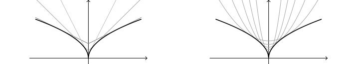
Figure 1. Majorization of the function $\varphi(t)=\sqrt{|{t}|}$ by shifted and scaled absolute values (left) and quadratics (right).

In the first case (3.1), the minimization problem becomes

$$\min_{x,s\geq 0}\frac{1}{2}\|{Ax-y}\|^{2}+\sum_{k=1}^{\infty}(s_{k}|x_{k}|^{2}+\psi_{k}(s_{k})).$$

The minimization over $x$ is now a quadratic problem and the minimization over $s$ decouples over $k$, thus yielding simple one-dimensional minimization problems. Note that the minimization over $s$ and $x$ simultaneously is still difficult, but alternating minimization is comparably simpler. In the second case (3.2), one would get

$$\min_{x,s\geq 0}\frac{1}{2}\|{Ax-y}\|^{2}+\sum_{k=1}^{\infty}(s_{k}|x_{k}|+\tilde{\psi}_{k}(s_{k})).$$

The minimization over $x$ is an $\ell^{1}$-penalized least squares problem, for which a number of methods is available [50, 26, 11, 38, 10, 28, 29, 56], while the minimization over $s$, again, decouples over $k$.

Note that equations (3.1) and (3.2) resemble the definition of the convex conjugate (basically up to sign changes). For example, one can see that $\psi_{k}$ from (3.2) fulfills $\psi_{k}(t)=-(-\phi_{k})^{*}(-t)$, where $(-\phi_{k})^{*}$ is the usual convex conjugate. Since the multiple minus-signs can be confusing, we present in the following a special notion of duality in the case of concave increasing functions.

We did not find a reference that contains all the necessary results regarding the concave conjugate and the superdifferential notions for concave functions. Thus, a presentation of this theory is included for the sake of completeness. It will be largely along the lines of convex duality and hence, most proofs can be omitted.

We will investigate the following set of functions:

$$\mathrm{CI}=\{\psi:[0,\infty)\to[-\infty,\infty)\ \mid\psi\ \text{concave and increasing}\}.$$

For $\psi\in\mathrm{CI}$, define

$$\operatorname{maj}(\psi)=\{(t,l)\in[0,\infty)\times[-\infty,\infty)\ \mid st+l\geq\psi(s),\,\forall s\geq 0\}.$$

The pairs $(t,l)\in\operatorname{maj}(\psi)$ parametrize the linear functions on $[0,\infty)$ which majorize $\psi$, where $t$ is its slope and $l$ is the intercept. Note that this construction is analogous to the situation of the convex conjugate where one shows that a convex and lower semi-continuous function is exactly the supremum of all affine functions below it. This leads to the well known duality theory for convex functions. An adaptation to the situation of concave increasing functions provides us with the following results.

Proposition 3.1.

For any subset $M\subset[0,\infty)\times[-\infty,\infty)$, it holds that the function

$$\varphi(s)=\inf_{(t,l)\in M}st+l$$

defined on $[0,\infty)$ is in $CI$.

Moreover, every function $\psi\in CI$ can be written as

$$\psi(s)=\inf_{(t,l)\in\operatorname{maj}(\psi)}st+l.$$

Proof.

Most of the claim follows by analogy to the convex case. The only thing which is missing is the monotonicity, that can be seen as follows: If $s_{1}\leq s_{2}$, then (since $t\geq 0$) $s_{1}t+l\leq s_{2}t+l$ for all $(t,l)\in M$. This shows that $\varphi(s_{1})\leq\varphi(s_{2})$. ∎

Definition 3.2.

For $\psi\in CI$, the concave conjugate is defined by

$$\psi^{\oplus}(t)=\inf_{s\geq 0}\big{(}st-\psi(s)\big{)}.$$

It is clear that $\psi^{\oplus}\in CI$.

Proposition 3.3.

For all $\psi\in CI$, one has ${\psi^{\oplus}}^{\oplus}=\psi$.

We introduce a notion of supergradient for functions in $CI$ (see also [9]):

Definition 3.4.

For $\psi\in CI$, we say that $s^{*}\geq 0$ is a supergradient of $\psi$ at $s$, if for all $r\geq 0$ it holds that

$$\psi(s)+s^{*}(r-s)\geq\psi(r).$$

We denote the set of all such $s^{*}$ by ${\hat{\partial}}\psi(s)$ and call it superdifferential.

Note that ${\hat{\partial}}\psi(s)=-{\partial}(-\psi)(s)$, where $\partial(-\psi)$ is the subdifferential of the convex function $-\psi$.

Theorem 3.5 (Fenchel inequality and Fenchel equality).

For $\psi\in CI$, one has

$$\psi(s)+\psi^{\oplus}(s^{*})\leq ss^{*},\quad\forall s\geq 0,s^{*}\geq 0.$$

Moreover, $\psi(s)+\psi^{\oplus}(s^{*})=ss^{*}$ if and only if $s^{*}\in\hat{\partial}\psi(s)$ (or, equivalently $s\in\hat{\partial}\psi^{\oplus}(s^{*})$).

Proof.

The inequality follows from

$$\psi(s)+\psi^{\oplus}(s^{*})=\psi(s)+\inf_{r\geq 0}(rs^{*}-\psi(r))\leq\psi(s)+ss^{*}-\psi(s).$$

For the equality, note that $s^{*}\in\hat{\partial}\psi(s)$ is by definition equivalent to the inequality

$$\psi(s)-ss^{*}\geq\psi(r)-s^{*}r,\ \text{for all $r\geq 0$}.$$

In turn, this is equivalent to

$$\psi(s)-ss^{*}\geq\sup_{r\geq 0}(\psi(r)-s^{*}r)=-\psi^{\oplus}(s^{*})$$

which is the same as $\psi(s)+\psi^{\oplus}(s^{*})\geq ss^{*}$. The claim follows with Fenchel’s inequality. ∎

As an example, we take $\psi(s)=s^{p}$ with $0<p<1$. The concave conjugate is

$$\psi^{\oplus}(t)=\inf_{s\geq 0}(st-\psi(s))=\inf_{s\geq 0}(st-s^{p}).$$

The infimum is attained at $s=(t/p)^{1/(p-1)}$ and the value evaluates to

$$\psi^{\oplus}(t)=\Big{(}\tfrac{1}{p^{1/(p-1)}}-\tfrac{1}{p^{p/(p-1)}}\Big{)}t^{p/(p-1)}.$$

The special case $p=1/2$, for example, leads to $\psi^{\oplus}(t)=-1/(4t)$ and hence, by Proposition 3.3 we have the representation

$$\sqrt{s}=\inf_{t\geq 0}\left(st+\tfrac{1}{4t}\right).$$

4. Iteratively reweighted quadratic regularization

This section uses the concave conjugate to derive flexible majorization approaches which lead to simple minimization algorithms for the regularized problems. A noteworthy property of these methods is their monotonicity, in the sense that they decrease the objective function in every iteration. We consider iterative $\ell^{2}$-minimization (i.e., quadratic Tikhonov regularization) in an infinite dimensional setting and develop the concept into a full algorithmic framework. Moreover, the resulting monotone algorithm will be tested on two examples, showing its efficiency and accuracy.

To get a series of quadratic problems, we write our objective function as

$$\min_{x}\|{Ax-y}\|^{2}+\alpha\sum_{k=1}^{\infty}\psi_{k}(|{x_{k}}|^{2}).$$

with $\psi_{k}\in\mathrm{CI}$ for all $k$. Again, using concave conjugates, we get

$$\min_{x\geq 0}\Big{[}\|{Ax-y}\|^{2}+\alpha\sum_{k=1}^{\infty}s_{k}|{x_{k}}|^{2}-\psi_{k}^{\oplus}(s_{k})\Big{]}.$$ (4.1)

If we alternatively minimize for $x$ and $s$, we get

1. Initialize with some $x^{0}$ and $s^{0}$, set $n=0$ and iterate

2. Obtain $x^{n+1}$ by solving $A^{*}(Ax-y)+\alpha\operatorname{diag}(s^{n})x=0$

3. $s_{k}^{n+1}\in\hat{\partial}\psi_{k}(|{x_{k}^{n+1}}|^{2})$.

The next lemma shows that the method is indeed of descent type and quantifies the guaranteed descent in each step.

Lemma 4.1.

Let $F(x)=\|{Ax-y}\|^{2}+\alpha\sum_{k}\psi_{k}(|{x_{k}}|^{2})$ and let $x^{n}$ be the iterates of the above iteration. Then it holds that

$$F(x^{n+1})\leq F(x^{n})-\|{Ax^{n+1}-Ax^{n}}\|^{2}-\alpha\sum_{k}s_{k}^{n}(x_{k}^{n}-x_{k}^{n+1})^{2}.$$

Proof.

We write (using $A^{*}(Ax^{n+1}-y)=-\alpha\operatorname{diag}(s^{n})x^{n+1}$)

$$F(x^{n})-F(x^{n+1}) =\|{Ax^{n}-y}\|^{2}-\|{Ax^{n+1}-y}\|^{2}+\alpha\sum_{k}\psi_{k}(|{x_{k}^{n}}|^{2})-\psi_{k}(|{x_{k}^{n+1}}|^{2})$$

$$=\|{Ax^{n}-Ax^{n+1}}\|^{2}+\langle{x^{n}-x^{n+1}},{A^{T}(Ax^{n+1}-y)}\rangle+\alpha\sum_{k}\psi_{k}(|{x_{k}^{n}}|^{2})-\psi_{k}(|{x_{k}^{n+1}}|^{2})$$

$$=\|{Ax^{n}-Ax^{n+1}}\|^{2}++\alpha\sum_{k}\psi_{k}(|{x_{k}^{n}}|^{2})-\psi_{k}(|{x_{k}^{n+1}}|^{2})-s_{k}^{n}x_{k}^{n+1}(x_{k}^{n}-x_{k}^{n+1}).$$

Now we use that $\psi_{k}(t^{2})\leq st^{2}-\psi_{k}^{\oplus}(s)$ with $t=x_{k}^{n+1}$ and $s=s_{k}^{n}$ to get

$$F(x^{n})-F(x^{n+1}) \geq\|{Ax^{n}-Ax^{n+1}}\|^{2}+\alpha\sum_{k}\psi_{k}(|{x_{k}^{n}}|^{2})-s_{k}^{n}(x_{k}^{n+1})^{2}+\psi_{k}^{\oplus}(s_{k}^{n})-s_{k}^{n}x_{k}^{n+1}(x_{k}^{n}-x_{k}^{n+1}).$$

By the Fenchel equality (Theorem  3.5) and since $s_{k}^{n}\in\hat{\partial}\psi_{k}(|{x_{k}^{n}}|^{2})$ we have that $\psi_{k}(|{x_{k}^{n}}|^{2})+\psi_{k}^{\oplus}(s_{k}^{n})=s_{k}^{n}|{x_{k}^{n}}|^{2}$ and thus

$$F(x^{n})-F(x^{n+1}) \geq\|{Ax^{n}-Ax^{n+1}}\|^{2}+\alpha\sum_{k}s_{k}^{n}|{x_{k}^{n}}|^{2}-s_{k}^{n}|{x_{k}^{n+1}}|^{2}-s_{k}^{n}x_{k}^{n+1}(x_{k}^{n}-x_{k}^{n+1})$$

$$=\|{Ax^{n}-Ax^{n+1}}\|^{2}+\alpha\sum_{k}s_{k}^{n}(x_{k}^{n}-x_{k}^{n+1})^{2}.$$

∎

Lemma 4.2.

For the iterates $x^{n}$, $s^{n}$, it holds that

1. $(F(x^{n}))$ is convergent,

2. $\displaystyle{\sum_{n=0}^{\infty}\|{A(x^{n+1}-x^{n})}\|^{2}\leq F(x^{0})}$,

3. $\displaystyle{\sum_{n=0}^{\infty}\sum_{k=1}^{\infty}s^{n}_{k}(x^{n+1}_{k}-x^{n}_{k})^{2}\leq F(x^{0})/\alpha}$,

4. $\displaystyle{\|{A(x^{n+1}-x^{n})}\|\to 0}$ for $n\to\infty$, and

5. $\displaystyle{\sum_{k=1}^{\infty}s^{n}_{k}(x^{n+1}_{k}-x^{n}_{k})^{2}\to 0}$ for $n\to\infty$.

Proof.

Summing up the inequalities from Lemma 4.1 for $n=0$ to $m$, we get

$$F(x^{m+1})\leq F(x^{0})-\sum_{n=0}^{m}\|{A(x^{n+1}-x^{n})}\|^{2}-\alpha\sum_{n=0}^{m}\sum_{k}s^{n}_{k}(x^{n}_{k}-x^{n+1}_{k})^{2}$$

from which the claim follows. ∎

The above lemma does not show convergence of the sequence of iterates yet. This could, in principle, be shown by adapting results from [59]. We do not pursue this here further, but instead, consider the special case of flexible penalties with varying exponents $p_{k}$ in the next section.

5. A monotone algorithm for the regularized problem

In this section, the previous approach by iterative $\ell^{2}$-regularization will be developed into a full algorithmic framework. For simplicity, we will focus on the case where all functions $\phi_{k}$ are of type $\phi_{k}(t)=t^{p_{k}}$ and will propose an algorithm to solve the minimization problem

$$\min_{x\in\ell^{p_{k}}}\frac{1}{2}||Ax-y||^{2}+\alpha\sum_{k\in\mathbb{N}}|x_{k}|^{p_{k}},$$ (5.1)

with $\displaystyle{\ell^{p_{k}}:=\{x=(x_{k}):\,\sum_{k\in\mathbb{N}}|x_{k}|^{p_{k}}<\infty\}}$ and $(p_{k})\subset(0,1)$. The behavior of the algorithm using other $\phi_{k}$ functionals will be discussed in the numerics subsection.

5.1. Convergence properties

Assume that $\displaystyle{\inf_{k\in\mathbb{N}}p_{k}>0}.$

We actually consider a slightly different version of the quadratic approximation from (4.1). That is, we minimize over $x$ the following regularized functional

$$J_{\varepsilon}(x)=\frac{1}{2}||Ax-y||^{2}+\alpha\sum_{k}\Psi_{\varepsilon,p_{k}}(|x_{k}|^{2}),$$ (5.2)

where for $\varepsilon>0$, $t\geq 0$ and $p\in(0,1)$,

$$\Psi_{\varepsilon,p}(t)=\left\{\begin{array}[]{ll}\frac{p}{2}\frac{t}{\varepsilon^{2-p}}&\mbox{for }\,\,0\leq t\leq\varepsilon^{2}\\ \vskip 3.0pt plus 1.0pt minus 1.0pt\cr t^{\frac{p}{2}}-(1-\frac{p}{2})\varepsilon^{p}&\mbox{ for }\,\,t\geq\varepsilon^{2}.\end{array}\right.\,$$ (5.3)

Figure 2. The function $\Psi_{\varepsilon,p}$ from (5.3) for different values of $\varepsilon$.

That is,

$$J_{\varepsilon}(x)=\frac{1}{2}||Ax-y||^{2}+\alpha\sum_{|x_{k}|\geq\varepsilon}\Big{(}|x_{k}|^{p_{k}}-(1-\tfrac{p_{k}}{2})\varepsilon^{p_{k}}\Big{)}+\alpha\sum_{|x_{k}|\leq\varepsilon}\left(\frac{p_{k}}{2\varepsilon^{2-p_{k}}}|x_{k}|^{2}\right).$$ (5.4)

Note that $\Psi_{\varepsilon,p}$ is well defined, differentiable, and concave. Clearly, $J_{\varepsilon}$ has minimizers in $\ell^{2}$. The necessary optimality condition is given by

$$A^{*}Ax+\frac{\alpha p}{\max(\varepsilon^{2-p},|x|^{2-p})}x=A^{*}y,$$ (5.5)

where the second addend is short for the sequence with component $\frac{\alpha p_{k}}{\max(\varepsilon^{2-p_{k}},|x_{k}|^{2-p_{k}})}x_{k}$. Note that the optimality condition (5.5) identifies local minimizers.

In order to solve (5.5), the following iterative procedure is considered:

$$A^{*}Ax^{i+1}+\frac{\alpha p}{\max(\varepsilon^{2-p},|x^{i}|^{2-p})}x^{i+1}=A^{*}y,\,{i\in\mathbb{N},}$$ (5.6)

where nonlinear functions are applied component-wise in the second addend that has components $\frac{\alpha p_{k}}{\max(\varepsilon^{2-p_{k}},|x_{k}^{i}|^{2-p_{k}})}x_{k}^{i+1}$. Note that (5.6) is well defined.

We have the following convergence result.

Theorem 5.1.

For $\varepsilon>0$, let $(x^{i})$ be generated by (5.6). Then $(J_{\varepsilon}(x^{i}))$ is strictly monotonically decreasing, unless there exists some $i$ such that $x^{i}=x^{i+1}$, and $x^{i}$ satisfies the necessary optimality condition (5.5). Moreover, every cluster point of $(x^{i})$, of which there exists at least one, is a solution of (5.5).

Proof.

The proof follows similar arguments to that of Theorem 4.1 in [32] and of Lemma 4.1. For the sake of completeness, we sketch the main proof steps. By applying (5.6) to $x^{i+1}-x^{i}$, we get

$$\frac{1}{2}\|Ax^{i+1}\|^{2}-\frac{1}{2}\|Ax^{i}\|^{2}+\frac{1}{2}\|A(x^{i+1}-x^{i})\|^{2}+\alpha\left\langle\frac{p}{\max(\varepsilon^{2-p},|x^{i}|^{2-p})}x^{i+1},x^{i+1}-x^{i}\right\rangle\\ =\langle A^{*}y,x^{i+1}-x^{i}\rangle.$$

Note that

$$\left\langle\frac{p}{\max(\varepsilon^{2-p},|x^{i}|^{2-p})}x^{i+1},x^{i+1}-x^{i}\right\rangle=\frac{1}{2}\sum_{k\in\mathbb{N}}\frac{p_{k}(|x^{i+1}_{k}|^{2}-|x^{i}_{k}|^{2}+|x^{i+1}_{k}-x_{k}^{i}|^{2})}{\max(\varepsilon^{2-p_{k}},|x^{i}_{k}|^{2-p_{k}})}$$ (5.7)

and

$$\frac{1}{2}\frac{p_{k}}{\max(\varepsilon^{2-p_{k}},|x^{i}_{k}|^{2-p_{k}})}(|x^{i+1}_{k}|^{2}-|x^{i}_{k}|^{2})=\Psi_{\varepsilon,p_{k}}^{\prime}(|x_{k}^{i}|^{2})(|x^{i+1}_{k}|^{2}-|x^{i}_{k}|^{2}).$$ (5.8)

Since $\Psi_{\varepsilon,p_{k}}$ is concave, we have

$$\Psi_{\varepsilon,p_{k}}(|x^{i+1}_{k}|^{2})-\Psi_{\varepsilon,p_{k}}(|x^{i}_{k}|^{2})-\frac{1}{2}\frac{p_{k}}{\max(\varepsilon^{2-p_{k}},|x^{i}_{k}|^{2-p_{k}})}(|x^{i+1}_{k}|^{2}-|x^{i}_{k}|^{2})\leq 0.$$ (5.9)

Then, using (5.7), (5.8), (5.9), we get

$$J_{\varepsilon}(x^{i+1})+\frac{1}{2}\|A(x^{i+1}-x^{i}\|^{2}+\frac{1}{2}\sum_{k\in\mathbb{N}}\frac{\alpha p_{k}}{\max(\varepsilon^{2-p_{k}},|x^{i}_{k}|^{2-p_{k}})}|x_{k}^{i+1}-x_{k}^{i}|^{2}\leq J_{\varepsilon}(x^{i}).$$ (5.10)

From (5.10) and coercivity of $J_{\varepsilon}$ it follows that $(x^{i}_{k})$ is bounded in $\ell^{2}$ and hence in $\ell^{\infty}$. This and $\displaystyle{\inf_{k\in\mathbb{N}}p_{k}>0}$ imply existence of a constant $\kappa>0$ such that

$$J_{\varepsilon}(x^{i+1})+\frac{1}{2}||A(x^{i+1}-x^{i})||^{2}+\kappa||x^{i+1}-x^{i}||^{2}\leq J_{\varepsilon}(x^{i}),$$ (5.11)

from which we conclude the first part of the theorem. From (5.11), we deduce that

$$\sum_{i}||A(x^{i+1}-x^{i})||^{2}+\kappa||x^{i+1}-x^{i}||^{2}<\infty.$$ (5.12)

Since $(x^{i})$ is bounded in $\ell^{2}$, there exists a subsequence $(x^{i_{l}})$ and $\bar{x}\in\ell^{2}$ such that $(x^{i_{l}})$ converges weakly to $\bar{x}$ in $\ell^{2}$. By (5.12) we have that $\displaystyle{\lim_{l\to\infty}x_{k}^{i_{l+1}}=\lim_{l\to\infty}x_{k}^{i_{l}}=\bar{x}_{k}}$. Testing (5.6) with $e_{k},k=1,\dots,$ and passing to the limit with respect to $i$ in (5.6), we get that $\bar{x}$ is a solution to (5.5). ∎

Remark 3.

Theorem 5.1 shows that each cluster point is stationary. The extension to global convergence under the Kurdyka-Lojasiewicz (KL) property seems a difficult task. We did not succeed to recover such a convergence, since it is not clear how to prove that $\psi\circ J_{\varepsilon}$ (where $\psi$ is the KL function) is a Lyapounov function with decreasing rate close to $||x^{i+1}-x^{i}||$, which is the key point on which the KL argument relies. Take, for example, a (classical) reference for the proof of the convergence under the KL property: Theorem $8$ of paper [3]. In the following inequality due to the KL property,

$$\psi^{\prime}(J_{\epsilon}(x^{i}))||\partial J_{\epsilon}(x^{i})||\geq 1,$$

one needs to estimate the lefthand side in terms of $||x^{i}-x^{i-1}||$. In our case, we have

$$\partial J_{\epsilon}(x^{i})=A^{*}Ax^{i}-A^{*}y+\frac{\alpha p}{\max\{\epsilon^{2-p},|x^{i}|^{2-p}\}}x^{i},$$

where

$$A^{*}Ax^{i}-A^{*}y=-\frac{\alpha p}{\max\{\epsilon^{2-p},|x^{i-1}|^{2-p}\}}x^{i}.$$

Hence,

$$\partial J_{\epsilon}(x^{i})=\frac{\alpha p}{\max\{\epsilon^{2-p},|x^{i}|^{2-p}\}}x^{i}-\frac{\alpha p}{\max\{\epsilon^{2-p},|x^{i-1}|^{2-p}\}}x^{i}$$

should be estimated in terms of $||x^{i}-x^{i-1}||$ for all $\epsilon>0$, which may not be possible.
Moreover we remark that the KL property has been proved for the $\ell^{p},p\in[0,1)$ nonconvex penalty (see [8], section $5$), but in the case of a flexible $\ell^{p_{k}},(p_{k})\in(0,1)$ penalty like ours, it is not straightforward (at least one would need some further assumptions on the sequence $p_{k}$, which we did not investigate in detail).

Remark 4.

Note that the same result holds true in finite dimension for the problem

$$\min_{x\in\mathbb{R}^{d}}\frac{1}{2}||Ax-y||^{2}+\alpha\sum_{k}|(\Lambda x)_{k}|^{p_{k}},$$ (5.13)

where $\Lambda\in\mathbb{R}^{m\times d}$. However, in order to have existence of a solution $\Lambda$ must satisfy some additional assumptions, e.g. $\mbox{Ker}(A)\cap\mbox{Ker}(\Lambda)=\{0\}$. The presence of such kind of operator was thoroughly investigated in [32], where the problem is finite dimensional. One main focus of [32] was an application in fracture mechanics, where the presence of the operator $\Lambda$ is crucial. In the present paper we are mostly interested in the analysis of the $p_{k}$-sequence approach, whose setting does not seem to provide any new insight into the fracture mechanics examples considered, e.g., in [32]. Indeed, in those kind of examples the regularization term is active just on one component of the solution. However, even though in the present paper we do not focus on the analysis of the case of an operator $\Lambda\neq I$ inside the regularization term, we remark that in the numerical tests such kind of operator could be used.

The following proposition establishes the convergence of minimizers of (5.2) to solutions of (5.1) as $\varepsilon$ goes to zero. The proof uses a technique similar to the one of Proposition 1 of [32]. As it is easily understandable from the above mentioned proof, we just underline that the following result gives an $\ell^{2}$-convergence of the sequence $(x_{\varepsilon})_{\varepsilon>0}$ as $\varepsilon\to 0$ to any cluster point.

Proposition 5.2.

Let $(x_{\varepsilon})_{\varepsilon>0}$ be solutions to (5.2). Then any cluster point of $(x_{\varepsilon})_{\varepsilon>0}$ as $\varepsilon\to 0^{+}$, of which there exists at least one, is a solution of (5.1).

5.2. Numerical results

In the sequel we investigate the performance of the monotone algorithm in practice. For this reason we will work in finite dimension. Our aims are showing the good performance of the $(p_{k})$ sequences approach in the monotone scheme, and comparing these results to the ones of [32] with $p$ fixed (and $\Lambda=I)$. Thus, we consider two problems that have been investigated also in [32]: the first one is an academic example where the operator $A$ is an $M$ matrix, and the second one is a time-dependent optimal control problem. We have tested two different kinds of penalty, first $\phi_{k}(t)=t^{p_{k}}$, and secondly $\phi_{k}(t)=\log(t^{p_{k}}+1)$. We describe our results in detail for the first case, and write some remarks on the second case, to underline the main differences.

Our findings show that the $(p_{k})$ sequences approach with $p_{k}\in(0,1)$ proves to be at least as effective as the $p$ fixed one (with $p\in(0,1)$), and in some cases, even more effective. Indeed, the $(p_{k})$ sequence approach is more flexible in the sense that it enables to concentrate the ”sparsity” constraint where it is more needed. We have exploited this feature in the control example in the way we have chosen the sequence $(p_{k})$. In this example, we are able to localise easily, a priori, an approximate region where the solution is known to be zero. Therefore we ”relax” the sparsity constraint by choosing sequences $(p_{k})$ which are closer to $1$ in those regions. In the areas where the solution is expected to be nonzero, we let the sequence tend towards the value used in [32] in the same situation. Choosing sequences as described above simplifies the scheme’s performance. Consistently with our expectations, the $(p_{k})$ sequence approach shows a smaller number of iterations and a lower residue as compared to the approach of [32] with $p$ fixed (see Table 2 and Table 3). Moreover, the $(p_{k})$ sequences approach provides better sparsity as compared to the approach of [32] with $p$ fixed (see Table 2 and Table 3).

The situation is a bit different in the academic $M$ matrix example, since we are not able to easily know a priori information on the behaviour of the solution. However, when testing different types of $(p_{k})\subset(0,1)$ sequences, we have observed more sparsity for sequences $p_{k}\to p$ where $p$ is the value used in [32]. For this reason, we will choose this type of sequences when comparing with the results of [32]. The aim of this experiment is to show the good performance of the $(p_{k})$ sequence approach in an academic example (with a residue always $O(10^{-9})$), and to show the different behaviour of the solution when changing the sequence $(p_{k})\subset(0,1)$.

For convenience of the exposition, we write the algorithm in the following form, see Algorithm $1$ for $\phi_{k}(t)=t^{p_{k}}$. A continuation strategy with respect to the parameter $\varepsilon$ is performed. In each of the following example, the initialization and range of $\varepsilon$-values will be described. The key modifications in the case $\phi_{k}(t)=\log(t^{p_{k}}+1)$ are described in Remark 5.

The algorithm stops when the $\ell^{\infty}$-norm of the residue of (5.5) is $O(10^{-8})$ in the M Matrix example and $O(10^{-15})$ in the time control problem example. At this instance, the $\ell^{2}$-residue is typically much smaller. Therefore, we find an approximate solution of the $\varepsilon$-regularized optimality condition (5.5). The system in (5.15) is solved through the MATLAB function mldivive (that is, the backslash command). The initialization $x^{0}$ is chosen as the solution of the problem (5.1) where the $\ell^{p_{k}}$-term is replaced by the $\ell^{2}$-norm, that is,

$$x^{0}=(A^{*}A+2\alpha)^{-1}A^{*}y.$$ (5.14)

Inspired by the findings of [32], we have observed that for some values of $\alpha$ the previous initialization is not suitable (that is, the obtained residue is too big). In order to overcome the problem, we have successfully tested a continuation strategy with respect to increasing $\alpha$-values.

Algorithm 1 Monotone algorithm + $\varepsilon$-continuation strategy

1:Initialize $\varepsilon=\varepsilon^{0}$, $x^{0}$ and $i=0$;

2:repeat

3:   Solve for $x^{i+1}$

$$A^{*}Ax^{i+1}+\frac{\alpha p}{\max(\varepsilon^{2-p},|x^{i}|^{2-p})}x^{i+1}=A^{*}y,$$ (5.15)

where the second addend is short for the vectors with component $\frac{\alpha p}{\max(\varepsilon^{2-p_{k}},|x^{i}_{k}|^{2-p_{k}})}x^{i+1}_{k}$.

4:   Set $i=i+1$.

5:until the stopping criterion is fulfilled.

6:Reduce $\varepsilon$ and repeat 2.

Remark 5.

When $\phi_{k}(t)=\log(t^{p_{k}}+1)$, the regularization (5.2) becomes

$$J_{\varepsilon}(x)=\frac{1}{2}||Ax-y||^{2}+\alpha\sum_{k\in\mathbb{N}}\log(\Psi_{\varepsilon,p_{k}}(|x_{k}|^{2})+1),$$

and equation (5.15) written in the following compact form becomes

$$(A^{*}A+FM)x^{i+1}=A^{*}y,$$

where $F$ is the diagonal matrix with $k$ component $\frac{1}{\Psi_{\varepsilon,p_{k}}(|x^{i}_{k}|^{2})+1}$ and $M$ is the diagonal matrix with $k$-component $\frac{\alpha p_{k}}{\max(\varepsilon^{2-p_{k}},|x_{k}^{i}|^{2-p_{k}})}$.

Note that, in the exposition of the numerical results, the total number of iterations shown in the tables takes into account the continuation strategy with respect to $\varepsilon$, but it does not take into account the continuation with respect to $\alpha$. Finally we underline that in all the tests described in the following, the value of the objective functional for each iteration was tested to be monotonically decreasing. Note that this is consistent with the result of Theorem 5.1.

In the sequel we will adopt the following notation. For $x\in\mathbb{R}^{d}$ we will denote $|x|_{0}=\#\{k\,:\,|x_{k}|>10^{-10}\},$ $|x|_{0}^{c}=\#\{k\,:\,|x_{k}|\leq 10^{-10}\},$ and by $||x||$ the euclidean norm of $x$.

5.2.1. M-Matrix example

Here the monotone scheme will be tested for the M-matrix example. This is a classical academic example that we have chosen to confirm the good performance of our scheme for different values of the sequence $(p_{k})\subset(0,1]$. More specifically, we consider

$$\min_{x\in\mathbb{R}^{d^{2}}}\frac{1}{2}||Ax-y||^{2}+\alpha\sum_{k=1}^{d^{2}}|x_{k}|^{p_{k}},$$ (5.16)

where $A$ is the backward finite difference gradient

$$A=(d+1)\left(\begin{array}[]{c}G_{1}\\ G_{2}\end{array}\right),$$ (5.17)

with $G_{1}\in\mathbb{R}^{d(d+1)\times d^{2}},G_{2}\in\mathbb{R}^{d(d+1)\times d^{2}}$ given by

$$G_{1}=I\otimes D,\quad G_{2}=D\otimes I.$$

Here $I$ is the $d\times d$ identity matrix, $\otimes$ denotes the tensor product and $D\in\mathbb{R}^{(d+1)\times d}$ is given by

$$D=\left(\begin{array}[]{ccccc}1&0&0&\cdots&0\\ -1&1&0&\cdots&0\\ \vspace{0.2cm}\hfil\\ 0&\cdots&0&-1&1\\ 0&\cdots&0&0&-1\end{array}\right).$$ (5.18)

Then $A^{*}A$ is an $M$ matrix coinciding with the $5$-point star discretization on a uniform mesh on a square of the Laplacian with Dirichlet boundary conditions. Note that (5.16) can be equivalently expressed as

$$\min_{x\in\mathbb{R}^{d^{2}}}\frac{1}{2}\|Ax\|^{2}-\langle x,f\rangle+\alpha\sum_{k=1}^{d^{2}}|x_{k}|^{p_{k}},$$ (5.19)

where $f=A^{*}y$. If $\alpha=0$, this is the discretized variational form of the elliptic equation

$$-\Delta z=f\mbox{ in }\Omega,\quad z=0\mbox{ on }\partial\Omega.$$ (5.20)

For $\alpha>0$, the variational problem (5.19) gives a solution with piecewise constant enhancing behaviour.

We choose $f$ as in [32], subsection $3.4$, namely $f$ is a discretization of

$f(x_{1},x_{2})=10x_{1}\mbox{sin}(5x_{2})\mbox{cos}(7x_{1})$. The parameter $\varepsilon$ varies in the same range as in [32], that is, it was initialized with $10^{-1}$ and decreased to $10^{-6}$.

In Table 5.2.1 we show the performance of Algorithm $1$ for $p\to 0.1$, $h=1/64$ as mesh size and $\alpha$ incrementally increasing by factor of $10$ from $10^{-4}$ to $10$. The sequence $(p_{k})$ is approximated by a vector of $N=63^{2}$ points with $p_{0}=1.1$, generated by the MATLAB command $(p_{k})=0.1+1./P$ with $P=linspace(1,100,N)$. In Figure 3 we show the graphics of the solutions for different values of $\alpha$ for which most changes occur.

One can observe significant differences with respect to different values of $\alpha$. The third row of Table 3 shows that $|x|^{c}_{0}$ increases with $\alpha$, as expected. For example, for $\alpha=1,10$, we have $|x|^{c}_{0}=3969$, or equivalently, $|x|_{0}=0$, that is, the solution to (5.19) is constantly zero. Moreover, we see that $|x|^{p}_{p}$ decreases when $\alpha$ increases (see the fourth row). In the fifth row we show the $\ell^{\infty}$ norm of the residue, which is $O(10^{-9})$ for all the considered $\alpha$.

Note also that the number of iterations is sensitive with respect to $\alpha$, in particular it increases for $\alpha$ increasing from $10^{-4}$ to $10^{-1}$ and it decreases consistently for $\alpha=1,10$.

The algorithm was also tested for different values of $(p_{k})\subset(0,1)$. The results obtained show dependence on $(p_{k})$. In particular in Figure 4 we show the graphics of the solution for $(p_{k})$ a random sequence, that is a vector of $N=63^{2}$ uniformly distributed random numbers in the interval $(0,1)$, obtained by the command rand in MATLAB. Comparing Figure 4 B) to Figure 3 B), we see that for $\alpha=0.1$ the solution is less sparse as compared to the solution for $p_{k}\to 0.1$.

For any $k$, we say that $k$ is a singular component of the vector $x$ if $k\in\{k\,:\,|x_{k}|<\varepsilon\}$. In particular, note that the singular components are the ones where the $\varepsilon$-regularization is most influential. In the sixth row of the tables we show $Sp$, which denotes the number of the singular components of $x$. Note that it coincides with the quantity $|x|_{0}^{c}$, which reassures the validity of the $\varepsilon$-strategy.

Moreover, we tested sequences $p_{k}\to 0$, but no significant improvement was remarked with respect to the above explained results. In part, this seems coherent with the results of [32] where $p=0$ was not tested successfully.

We tested the algorithm when $\phi_{k}(t)=\log(t^{p_{k}}+1)$, according to the modification shown in Remark 5. The results are shown in Figure 5 only in the case $\alpha=0.1$ and $\alpha=1$, since no significant changes are observed for smaller values of $\alpha$ with respect to $\alpha=0.1$. Comparing Figure 5 a) with Figure 3 b) and Figure 5 b) with Figure 3 c), the solution is less sparse. Moreover, the number of iterations and the residue are much higher with respect to $\phi_{k}(t)=t^{p_{k}}$, respectively of the order $10^{3}$ and $10^{-1}$.

Finally, we remark that if we modify the initialization (5.14), the method converges to the same solution with no remarkable modifications in the number of iterations, which is a sign for the global nature of the algorithm.

Table 1. $M$-matrix example, $p_{k}\to 0.1$, mesh size $h=\frac{1}{64}$. Results obtained by Algorithm $1$.

$\alpha$	$10^{-4}$	$10^{-3}$	$10^{-2}$	$10^{-1}$	$1$	10
no. of iterates	163	785	2046	1984	131	15
$|x|^{c}_{0}$	7	41	269	2617	3969	3969
$|x|^{p}_{p}$	$2*10^{3}$	$2*10^{3}$	$2*10^{3}$	$812$	9.6	7.3
Residue	$8*10^{-10}$	$8*10^{-9}$	$9*10^{-9}$	$4*10^{-9}$	$3*10^{-15}$	$10^{-15}$
$Sp$	7	41	269	2617	3869	3969

(a) $\alpha=0.01$

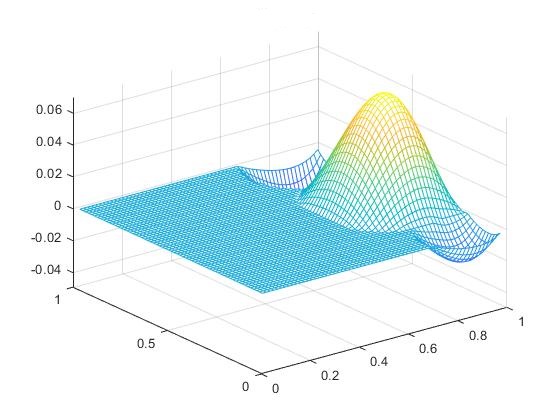
(b) $\alpha=0.1$

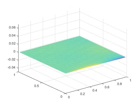
(c) $\alpha=1$

Figure 3. Solution of the M-matrix problem, $p_{k}\to^{+}0.1,$ mesh size $h=\frac{1}{64}$. Results obtained by Algorithm $1$.

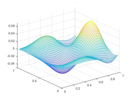
(a) $\alpha=0.01$

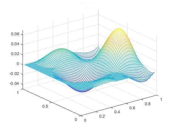
(b) $\alpha=0.1$

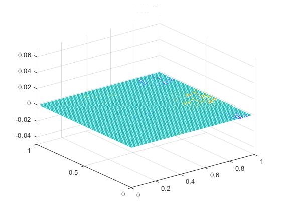
(c) $\alpha=1$

Figure 4. Solution of the M-matrix problem, $p_{k}\in(0,1]$ random sequence, mesh size $h=\frac{1}{64}$. Results obtained by Algorithm $1$.

(a) $\alpha=0.1$

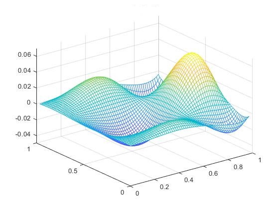
(b) $\alpha=1$

Figure 5. Solution of the M-matrix problem, $p_{k}\subset(0,1],p_{k}\to 0.1$, mesh size $h=\frac{1}{64}$. Results obtained by Algorithm $1$ as modified in Remark 5.

5.2.2. Time dependent control problem

The following example, of particular significance for our findings, is taken from [32], subsection $3.2$, to which we refer for further details. For the sake of completeness, we explain in the sequel the setting that we study. We consider the linear control system

$$\frac{d}{dt}z(t)=\mathcal{A}z(t)+Du(t),\quad z(0)=0,$$

that is,

$$z(T)=\int_{0}^{T}e^{\mathcal{A}(T-s)}Du(s)ds,$$ (5.21)

where the linear closed operator $\mathcal{A}$ generates a $C_{0}$-semigroup $e^{\mathcal{A}t}$, $t\geq 0$ on the state space $X$. More specifically, we consider the one-dimensional controlled heat equation for $z=z(t,x)$:

$$z_{t}=z_{xx}+d_{1}(x)u_{1}(t)+d_{2}(x)u_{2}(t),\quad x\in(0,1),$$ (5.22)

with homogeneous boundary conditions $z(t,0)=z(t,1)=0$ and thus $X=L^{2}(0,1)$. The differential operator $\mathcal{A}z=z_{xx}$ is discretized in space by the second order finite difference approximation with $n=49$ interior spatial nodes ($\Delta x=\frac{1}{50}$). We use two time dependent controls $\overrightarrow{u}=(u_{1},u_{2})$ with corresponding spatial control distributions $d_{i}$ chosen as step functions:

$$d_{1}(x)=\chi_{(.2,.3)},\quad d_{2}(x)=\chi_{(.6,.7)}.$$

The control problem consists in finding the control function $\overrightarrow{u}$ that steers the state $z(0)=0$ to a neighbourhood of the desired state $z_{T}$ at the terminal time $T=1$. We discretize the problem in time by the mid-point rule and we define the matrix $A$ as follows

$$A\overrightarrow{u}=\sum_{k=1}^{m}e^{\mathcal{A}\left(T-t_{k}-\frac{\Delta t}{2}\right)}(D\overrightarrow{u})_{k}\Delta t,$$ (5.23)

where $\overrightarrow{u}=(u_{1}^{1},\cdots,u_{1}^{m},u_{2}^{1},\cdots u_{2}^{m})$ is a discretized control vector whose coordinates represent the values at the mid-point of the intervals $(t_{k},t_{k+1})$. Note that in (5.23) we denote by $D$ a suitable rearrangement of the matrix $D$ in (5.21) with some abuse of notation. A uniform step-size $\Delta t=\frac{1}{50}$ ($m=50$) is utilized. More specifically, we apply our scheme to the discretized optimal control problem in time and space where $x$ from (5.1) is the discretized control vector $u\in\mathbb{R}^{2m}$ which is mapped by $A$ to the discretized output $z$ at time $1$ by means of (5.23) and $y$ in (5.1) is the discretized target function chosen as the Gaussian distribution $z_{T}(x)=0.4\,\mbox{exp}(-70(x-.7)^{2}))$ centered at $x=.7$. The parameter $\varepsilon$ was initialized with $10^{-3}$ and decreased down to $10^{-8}$. Since the second control distribution is well within the support of the desired state $z_{T}$, the authority of this control is expected to be stronger than that of the first one, which is away from the target.

The structure of the example allows us to exploit the flexibility of the $(p_{k})$ sequences approach since we know the two regions where the distributions of the control are active. Therefore we can ”relax” the sparsity constraint by choosing sequences $(p_{k})$ which are closer to $1$ in those regions, whereas in the areas where the solution is expected to be zero, we let the sequence tends towards the value used in [32] in the same situation.

More specifically, in Tables 2 and 3 we report the results of our tests for $p=0.5$ and $(p_{k})$ approximated by a vector of $N=100$ points with $p_{0}=0.51$ generated by the MATLAB command $(p_{k})=flip(0.5+1./P)$ with $P=linspace(2,100,N)$, respectively. In both tables, $\alpha$ is incrementally increasing by factor of $10$ from $10^{-2}$ to $1$. We report only the values for the second control $u_{2}$ since the first control $u_{1}$ is always zero. Note that the residue is always of the order of $10^{-15}$. Moreover, the quantity $|u_{2}|_{p}^{p}$ decreases for $\alpha$ increasing, as expected. In Table 2 we see that $|u_{2}|_{0}$ is always zero except that for $\alpha=10^{-2}$, whereas in Table 3 for $\alpha=10^{-1}$ it is different from zero. We remark , for smaller values of $\alpha$, we find values of $|u_{2}|_{0}$ different from zero (consistent with our expectation) also whit the $(p_{k})$ sequence. However, here we choose these values of $\alpha$ since we focus on the comparison between $(p_{k})$ and $p$ fixed and for these values of $\alpha$ we found the most interesting results. Consistently with our expectations, for each value of $\alpha$ the number of iterations and the residue are always smaller with the $(p_{k})$ sequence than for $p=0.5$ fixed. As an example, we refer to the first rows of Table 2 and Table 3 and we remark that the same holds true for different values of $\alpha$ than those of the above mentioned tables. As mentioned above, we believe that this improvement, as compared to the solution given by the $p$ fixed approach, resides in the fact that with $(p_{k})$ sequences we are able to give a ”different weight” to each component of the solution, thus simplifying the performance of the algorithm.

Moreover, we found some interesting improvements even with respect to the level of sparsity in the solution. In this regard, we underline that both $|u_{2}|_{0}^{c}$ and $|u_{2}|^{p_{k}}$ are smaller for $(p_{k})$ (see second and third rows of Table 2) than when $p=0.5$ is fixed ( see Table 3).

In the sixth row of the tables we show the number of singular components of the vector $u_{2}$ at the end of the $\varepsilon$-path following scheme, that is, $Sp:=\#\{i\,\,|\,\,|(u)_{2})_{i}|<\varepsilon\}$. For all considered values of $\alpha$, we have that $Sp$ is the same as $|u_{2}|_{0}^{c}$, thus confirming the effectiveness of the $\varepsilon$-strategy.

We tested the algorithm when $\phi_{k}(t)=\log(t^{p_{k}}+1)$, according to the modification shown in Remark 5. The results reported in Table 4 show that the algorithm works well enough in this case, too. However, for the tested value of $(p_{k})$, the performance is not as good as in the case where $\phi_{k}(t)=t^{p_{k}}$. Indeed, the residue is always bigger, the sparsity level of the solution is comparable but slightly smaller, and the number of iterates is slightly higher.

Finally, we remark that, if we change the initialization (5.14), the method converges to the same solution with no remarkable modifications in the number of iterations.

Table 2. Sparsity in a time-dependent control problem, $(p_{k})$, mesh size $h=\frac{1}{50}$. Results obtained by Algorithm $1$.

$\alpha$	$10^{-2}$	$10^{-1}$	$1$
no. of iterates	28	33	19
$|u_{2}|_{0}^{c}$	99	100	100
$|u_{2}|^{p}_{p}$	6	$10^{-6}$	$10^{-7}$
Residue	$10^{-17}$	$10^{-17}$	$10^{-18}$
Sp	99	100	100

Table 3. Sparsity in a time-dependent control problem, $p=0.5$, mesh size $h=\frac{1}{50}$. Results obtained by Algorithm $1$.

$\alpha$	$10^{-2}$	$10^{-1}$	$1$
no. of iterates	35	60	23
$|u_{2}|_{0}^{c}$	99	99	100
$|u_{2}|^{p}_{p}$	6.3	4.7	$10^{-6}$
Residue	$10^{-17}$	$10^{-11}$	$10^{-16}$
Sp	99	100	100

Table 4. Sparsity in a time-dependent control problem, $(p_{k})$, mesh size $h=\frac{1}{50}$. Results obtained by Algorithm $1$ modified as in Remark 5.

$\alpha$	$10^{-2}$	$10^{-1}$	$1$
no. of iterates	51	51	50
$|u_{2}|_{0}^{c}$	97	98	98
$|u_{2}|^{p}_{p}$	10	$1.9$	$0.7$
Residue	$10^{-1}$	$10^{-2}$	$10^{-2}$
Sp	97	98	98

6. Iteratively reweighted $\ell^{1}$-minimization

The analysis for the reweighted $\ell^{2}$-minimization cannot be directly adapted to the $\ell^{1}$-minimization case, because of the absolute value function singularity. Hence, the setting of this section is finite dimensional. The reader is referred also to [22], where the fixed exponent penalty case is dealt with.

If the problem under consideration is

$$\min_{x}\frac{1}{2}\|{Ax-y}\|^{2}+\alpha\sum_{k=1}^{N}\phi_{k}(|{x_{k}}|)$$

with $\phi_{k}\in CI$ for all $k$, then we can use the concave conjugates of the $\phi_{k}$ functions to formulate the problem as

$$\min_{x}\inf_{s_{k}\geq 0}\Big{[}G(x,s)=\frac{1}{2}\|{Ax-y}\|^{2}+\alpha\sum_{k=1}^{N}(s_{k}|{x_{k}}|-\phi_{k}^{\oplus}(s_{k}))\Big{]}.$$ (6.1)

Since $\phi_{k}$ is concave, $G$ in this problem is convex in $x$ and also convex in all the $s_{k}$ (jointly), but not convex in $x$ and $s_{k}$ jointly. However, we can perform alternating minimization:

1. Initialize with some $x^{0}$ and $s^{0}$, set $n=0$ and iterate

2. $\displaystyle{x^{n+1}\in\operatorname*{argmin}_{x}G(x,s^{n})}$

3. $\displaystyle{s^{n+1}\in\operatorname*{argmin}_{s\geq 0}G(x^{n+1},s)}$.

The minimization for $s$ decouples into one-dimensional problems $\displaystyle{\min_{s}(s|{x_{k}}|-\phi_{k}^{\oplus}(s))}$ with optimality conditions $0\in|{x_{k}}|+\partial(-\phi_{k}^{\oplus})(s)=|{x_{k}}|-\hat{\partial}\phi_{k}^{\oplus}(s)$. By Theorem 3.5, this holds if and only if $s\in\hat{\partial}\phi_{k}(|{x_{k}}|)$. We obtain the following method consisting of a sequence of convex $\ell^{1}$-minimization problems:

Initialize with some $x^{0}$ and $s^{0}$, set $n=0$ and iterate

$$x^{n+1}\in\operatorname*{argmin}_{x}\frac{1}{2}\|{Ax-y}\|^{2}+\alpha\sum_{k=1}^{N}s_{k}^{n}|{x_{k}}|$$ (6.2)

with

$$s_{k}^{n+1}\in\hat{\partial}\phi_{k}(|{x_{k}^{n+1}}|+\varepsilon).$$ (6.3)

Here, we allow for a shift $\varepsilon\geq 0$, since one may run into problems when $\hat{\partial}\phi_{k}(t)$ grows unbounded near zero (but still include $\varepsilon=0$ to be able to treat the general case).

Thus, we will work with a shifted version of the regularized problem, that is

$$F(x)=\frac{1}{2}\|{Ax-y}\|^{2}+\alpha\sum_{k=1}^{N}\phi_{k}(|{x_{k}}|+\varepsilon),\quad\varepsilon\geq 0.$$ (6.4)

We start the analysis of the method with a proposition on descent:

Proposition 6.1.

Assume that the functions $\phi_{k}$ are in $\mathrm{CI}$ and differentiable on $(0,\infty)$. Let $(x^{n})$ be generated by the algorithm (6.2)-(6.3). Then it holds

$$F(x^{n+1})\leq F(x^{n})-\frac{1}{2}\|{Ax^{n+1}-Ax^{n}}\|^{2}-\alpha D(x^{n+1},x^{n}),\,\forall n\in\mathbb{N},$$ (6.5)

where $D(x^{n+1},x^{n})$ is the sum of Bregman distances associated to the convex functions $-\phi_{k}$, that is

$${\sum_{k=1}^{N}D_{-\phi_{k}}}(|x_{k}^{n+1}|+\varepsilon,|x_{k}^{n}|+\varepsilon)=\sum_{k=1}^{N}\phi_{k}(|{x_{k}^{n}}|+\varepsilon)-\phi_{k}(|{x_{k}^{n+1}}|+\varepsilon)-s_{k}^{n}(|{x_{k}^{n}}|-|{x_{k}^{n+1}}|)$$

for some $s_{k}^{n}\in\hat{\partial}\phi_{k}(|x_{k}^{n}|+\varepsilon)$.

Proof.

Due to the optimality condition for $x^{n+1}$, there exists $\xi_{k}^{n+1}\in\partial(|\cdot|)(x^{n+1}_{k})$ such that

$$(A^{*}(Ax^{n+1}-y))_{k}+\alpha s_{k}^{n}\xi_{k}^{n+1}=0,\,\,1\leq k\leq N,$$ (6.6)

for some $s_{k}^{n}\in\hat{\partial}\phi_{k}(|{x_{k}^{n}}|+\varepsilon)$. Based on this, one has

$$F(x^{n})-F(x^{n+1}) = \frac{1}{2}\|Ax^{n}-Ax^{n+1}\|^{2}+\langle Ax^{n}-Ax^{n+1},Ax^{n+1}-y\rangle$$

$$+ \alpha\sum_{k=1}^{N}(\phi_{k}(|x_{k}^{n}|+\varepsilon)-\phi_{k}(|x_{k}^{n+1}|+\varepsilon))$$

$$= \frac{1}{2}\|Ax^{n}-Ax^{n+1}\|^{2}+\alpha\sum_{k=1}^{N}(x_{k}^{n+1}-x_{k}^{n})s_{k}^{n}\xi_{k}^{n+1}$$

$$+ \alpha\sum_{k=1}^{N}(\varphi_{k}(|x_{k}^{n}|+\varepsilon)-\varphi_{k}(|x_{k}^{n+1}|+\varepsilon))$$

$$\geq \frac{1}{2}\|Ax^{n}-Ax^{n+1}\|^{2}+\alpha\sum_{k=1}^{N}(|x_{k}^{n+1}|-|x_{k}^{n}|)s_{k}^{n}$$

$$+ \alpha\sum_{k=1}^{N}(\varphi_{k}(|x_{k}^{n}|+\varepsilon)-\varphi_{k}(|x_{k}^{n+1}|+\varepsilon))$$

$$= \frac{1}{2}\|Ax^{n}-Ax^{n+1}\|^{2}+\alpha\sum_{k=1}^{N}D_{-\varphi_{k}}(|x_{k}^{n+1}|+\varepsilon,|x_{k}^{n}|+\varepsilon).$$

Note that the last but one inequality followed from properties of subgradients of $|\cdot|$: $\xi_{k}^{n+1}x_{k}^{n}\leq|x_{k}^{n}|$ and $\xi_{k}^{n+1}x_{k}^{n+1}=|x_{k}^{n+1}|$. ∎

The next result shows convergence properties of the sequences generated by (6.2)-(6.3). We recall first a notion that will be used in the analysis, namely sequential consistency of functions. A convex function $g$ defined on a Banach spaces $X$ is called sequentially consistent on its domain if for any two sequences $(x^{k})$ and $(y^{k})$ such that the first is bounded, one has

$$D_{g}(y^{k},x^{k})\to 0\quad\Rightarrow\|x^{k}-y^{k}\|\to 0,\quad\mbox{as}\,\,k\to\infty.$$ (6.8)

There are several equivalent definitions for sequential consistency - see, e.g. Theorem 2.10 in [16]. Here we will take advantage of the following:

Let $g:\mathbb{R}^{N}\to(-\infty,\infty]$ be convex, lower semicontinuous, Fréchet differentiable on its domain, such that its derivative is uniformly continuous on bounded sets. Then $g$ is sequentially consistent.

We also recall the notion of stationary point for a locally Lipschitz functional. According to [24, Chapter 2], if $f:X\to\mathbb{R}$ is a locally Lipschitz function defined on a Banach space $X$, the generalized subdifferential of $f$ at $x\in X$ in the sense of Clarke is defined by

$$\partial f(x)=\{\xi\in X^{*}:f^{\circ}(x,v)\geq\langle\xi,v\rangle,\,\forall v\in X\},$$

where $f^{\circ}(x,v)$ is the Clarke directional derivative

$$f^{\circ}(x,v)=\limsup_{\begin{subarray}{c}y\to x\\ t\searrow 0\end{subarray}}\frac{f(y+tv)-f(y)}{t}\,.$$

A point $x\in X$ is called a stationary point of $f$, if $0\in\partial f(x).$ As expected, any local minimum point of $f$ is also a stationary point of the function.

In the remaining part of this section, we assume that the functions $t\to\phi_{k}(t+\varepsilon)$ are Lipschitz for any $\varepsilon>0$ (i.e., $\phi_{k}$ are uniformly Lipschitz on sets away from zero).Consequently, the mapping $\displaystyle\tilde{\phi}(x)=\sum_{k=1}^{N}\phi_{k}(|{x_{k}}|+\varepsilon)$ is also Lipschitz. Since the least squares term of $F$ is continuously differentiable and the regularizer is Lipschitz, it follows that the Clarke subdifferential of $F$ is additive, that is $\partial F(x)=A^{*}(Ax-y)+\partial\tilde{\phi}(x)$, where the latter Clarke sudifferential is given by $\partial\tilde{\phi}(x)=((\phi_{k}^{\prime}(|x_{k}|+\varepsilon)\xi_{k})_{k}$ with $\xi_{k}\in\partial(|\cdot|)(x_{k})$.

Proposition 6.2.

Let $\varepsilon>0$. Let the functions $\phi_{k}$ be in $CI$, coercive and continuously differentiable. Assume that the functions $-\phi_{k}$ are sequentially consistent on domains that are bounded and away from zero. Then each sequence $(x^{n})$ defined by (6.2) is bounded and verifies $\displaystyle{\lim_{n\to\infty}(x^{n+1}-x^{n})=0}$. Moreover, each accumulation point of $(x^{n})$ is a stationary point of the function $F$.

Proof.

The sequence $(F(x^{n}))$ is convergent, as it is decreasing due to (6.5), and is bounded from below. Thus, it yields

$$\lim_{n\to\infty}D(x^{n+1},x^{n})=0,\quad\lim_{n\to\infty}\|Ax^{n}-Ax^{n+1}\|=0.$$ (6.9)

Consequently,

$$\lim_{n\to\infty}D_{-\phi_{k}}(|x_{k}^{n+1}|+\varepsilon,|x_{k}^{n}|+\varepsilon)=0,\quad\forall k\in\mathbb{N},$$ (6.10)

which yields

$${\lim_{n\to\infty}\left(|x_{k}^{n+1}|-|x_{k}^{n}|\right)=0}$$ (6.11)

for each $k$, due to the sequential consistency of $-\phi_{k}$ for any $k$ on sets that are bounded and away from zero. Here we used the boundedness of $(x^{n})$ (that is implied by the boundedness of $(F(x^{n}))$) and an argument as in the proof of Lemma 2.2,

$$\frac{c}{1+L}\|x^{n}\|_{1}\leq\sum_{k=1}^{N}\frac{c|x_{k}^{n}|}{1+|x_{k}^{n}|}\leq c\sum_{k=1}^{N}\frac{|x_{k}^{n}|+\varepsilon}{1+|x_{k}^{n}|+\varepsilon}\leq\sum_{k=1}^{N}\phi_{k}(|x_{k}^{n}|+\varepsilon)\leq F(x^{n}).$$

Now (6.11) and the Lipschitz continuity of $\displaystyle x\mapsto\sum_{k=1}^{N}\phi_{k}(|x_{k}|+\varepsilon)$ combined with the second equality in (6) lead to

$$\lim_{n\to\infty}\left(x_{k}^{n+1}-x_{k}^{n}\right)\xi_{k}^{n+1}=0$$ (6.12)

for each $k$.

Fix $k\in\{1,\dots,N\}$. One distinguishes two cases. If $x_{k}^{n+1}\neq 0$ except for finitely many $n\in\mathbb{N}$, then $|\xi_{k}^{n+1}|=1$, which due to (6.12) implies that

$$\lim_{n\to\infty}\left(x_{k}^{n+1}-x_{k}^{n}\right)=0.$$ (6.13)

In the other case, there is a subsequence $(x_{k}^{n_{j}+1})$ which is constant zero. Since

$\displaystyle{\lim_{n\to\infty}\left(|x_{k}^{n+1}|-|x_{k}^{n}|\right)=0}$, one has $x_{k}^{n_{j}}\to 0$ and hence, $\displaystyle{\lim_{j\to\infty}(x_{k}^{n_{j}+1}-x_{k}^{n_{j}})=0}$.

Let $(x^{n_{j}})$ be a subsequence which converges to $\bar{x}$ and fix $k\in\{1,\dots,N\}$. By keeping the same notation on a subsequence of the bounded sequence $(\xi^{n_{j}}_{k})$, the closeness of the graph of the subdifferential of $|\cdot|$ (see, e.g. Theorem 24.4 in [51]) yields existence of $\xi_{k}\in\partial(|\cdot|)(\bar{x}_{k})$, such that $\xi^{n_{j}}_{k}\to\xi_{k}$ when $j\to\infty$. Due to (6.6), it follows that

$$(A^{*}(Ax^{n_{j}}-y))_{k}+\alpha\phi_{k}^{\prime}(|x_{k}^{n_{j}-1}-x_{k}^{n_{j}}+x_{k}^{n_{j}}|+\varepsilon)\xi_{k}^{n_{j}}=0,\,1\leq k\leq N.$$ (6.14)

By taking limit for $j\to\infty$ in (6.14) and using the continuity of $\phi^{\prime}_{k}$ imply that $\bar{x}$ is a stationary point of $F$. ∎

Remark 6.

The functions from Remark 1 satisfy the sequential consistency property on sets that are bounded and away from zero, since the component functions are twice differentiable with bounded second derivatives, and thus, their derivatives are Lipschitz on sets that are bounded and away from zero.

7. Conclusions

We proposed a general nonconvex approach to reconstruct sparse solutions of ill-posed problems with the aim of enhancing more flexibility than in the classical regularization penalties in $\ell^{p}$ spaces with $p\in(0,\infty)$. Our analysis touched both theoretical and numerical aspects. From a theoretical point of view, we studied the convergence of the regularization method and the convergence properties of a couple of majorization techniques, leading to monotone $\ell^{2}$-minimization and $\ell^{1}$-minimization schemes. Finally, we showed convergence of an algorithm based on $\ell^{2}$-minimization and tested it in two situations, first for an academic example where the operator is an M matrix, and secondly for a time-dependent optimal control problem. As shown by numerical results, the procedure is efficient and accurate, highlighting the advantages of using variable penalties over a fixed penalty.

Further work will concern a different numerical approach, that is, a primal dual active set method for the nonconvex problem. This method is inspired by the one proposed in [32] to study nonconvex problems with an $\ell^{p}$ penalty, $p\in(0,1]$. From a theoretical point of view, the primal dual active set method is interesting in itself since it identifies global minimizers (see Remark 5 of [32]). Moreover, the method seems to be more numerically effective than the monotone algorithm in some situations. Last but not least, learning the flexible regularizers is a challenging open problem.

8. Acknowledgments

The authors are grateful to Robert Csetnek (University of Vienna) for the discussions on generalized subdifferentials, and to the referee for the interesting comments and suggestions. The work of D.L. has been supported by the ITN-ETN project TraDE-OPT funded by the European Union’s Horizon 2020 research and innovation programme under the Marie Skłodowska-Curie grant agreement No 861137. This work represents only the author’s view and the European Commission is not responsible for any use that may be made of the information it contains. Furthermore, D.L. acknowledges funding from BMBF under grant 05M20MBB and from the DFG under grants LO 1436/9-1 and FOR 3022/1.

References

- [1] R. Akgün and Y.E. Yildirir. Convolution and Jackson inequalities in Musielak–Orlicz spaces. Turkish Journal of Mathematics, 42:2166–2185, 2018.
- [2] Marc Allain, Jérôme Idier, and Yves Goussard. On global and local convergence of half-quadratic algorithms. IEEE Transactions on Image Processing, 15(5):1130–1142, 2006.
- [3] Hédy Attouch, Jérôme Bolte, Patrick Redont, and Antoine Soubeyran. Proximal alternating minimization and projection methods for nonconvex problems: an approach based on the Kurdyka-łojasiewicz inequality. Math. Oper. Res., 35(2):438–457, 2010.
- [4] Amir Beck and Nadav Hallak. Optimization problems involving group sparsity terms. Mathematical Programming Series A, 178:39–67, 2019.
- [5] Yun bin Zhao and Duan Li. Reweighted ‘1-minimization for sparse solutions to underdetermined linear systems. SIAM Journal on Optimization, pages 1065–1088, 2012.
- [6] Michael J. Black and Anand Rangarajan. On the unification of line processes, outlier rejection, and robust statistics with applications in early vision. Int. J. Comput. Vis., 19:57–91, 1996.
- [7] Michael J Black and Anand Rangarajan. On the unification of line processes, outlier rejection, and robust statistics with applications in early vision. International journal of computer vision, 19(1):57–91, 1996.
- [8] Jérôme Bolte, Shoham Sabach, and Marc Teboulle. Proximal alternating linearized minimization for nonconvex and nonsmooth problems. Math. Program., 146(1-2, Ser. A):459–494, 2014.
- [9] K.C. Border. Supergradients - lecture notes, 2001. available at http://www.its.caltech.edu/kcborder/Notes/Supergrad.pdf.
- [10] Kristian Bredies and Dirk A. Lorenz. Iterated hard shrinkage for minimization problems with sparsity constraints. SIAM Journal on Scientific Computing, 30(2):657–683, 2008. [doi].
- [11] Kristian Bredies and Dirk A. Lorenz. On the convergence speed of iterative methods for linear inverse problems with sparsity constraints. Journal of Physics: Conference Series, 124:012031 (12pp), September 2008.
- [12] Kristian Bredies and Dirk A. Lorenz. Regularization with non-convex separable constraints. Inverse Problems, 25(8):085011 (14pp), 2009.
- [13] Kristian Bredies, Dirk A. Lorenz, and Stefan Reiterer. Minimization of non-smooth, non-convex functionals by iterative thresholding. Journal of Optimization Theory and Applications, 165(1):78–112, 2015.
- [14] Kristian Bredies, Dirk A. Lorenz, and Stefan Reiterer. Minimization of non-smooth, nonconvex functionals by iterative thresholding. J. Optim. Theory Appl., 165(1):78–112, 2015.
- [15] Luis M Briceno-Arias, Patrick L Combettes, J-C Pesquet, and Nelly Pustelnik. Proximal algorithms for multicomponent image recovery problems. Journal of Mathematical Imaging and Vision, 41(1):3–22, 2011.
- [16] Dan Butnariu and Elena Resmerita. Bregman distances, totally convex functions, and a method for solving operator equations in banach spaces. Abstract and Applied Analysis, 2006:084919, 2006.
- [17] Lotfi Chaâri, Jean-Christophe Pesquet, Amel Benazza-Benyahia, and Philippe Ciuciu. Minimization of a sparsity promoting criterion for the recovery of complex-valued signals. In SPARS’09-Signal Processing with Adaptive Sparse Structured Representations, 2009.
- [18] Raymond H Chan and Hai-Xia Liang. Half-quadratic algorithm for ell _p ell _q problems with applications to tv- image restoration and compressive sensing. In Efficient algorithms for global optimization methods in computer vision, pages 78–103. Springer, 2014.
- [19] Rick Chartrand. Exact reconstruction of sparse signals via noconvex minimization. IEEE Signal Processing Letters, 14(10):707–710, 2007.
- [20] Rick Chartrand. Fast algorithms for nonconvex compressive sensing: MRI reconstruction from very few data. 2009 IEEE International Symposium on Biomedical Imaging: From Nano to Macro, pages 262–265, 2009.
- [21] Scott Shaobing Chen, David L. Donoho, and Michael A. Saunders. Atomic decomposition by basis pursuit. SIAM Journal on Scientific Computing, 20(1):33–61, 1998.
- [22] Xiaojun Chen and Weijun Zhou. Convergence of the reweighted minimization algorithm for - minimization. Computational Optimization and Applications, 59(1-2):47–61, 2014.
- [23] Jon F. Claerbout and Francis Muir. Robust modeling with erratic data. Geophysics, 38(5):826–844, 1973.
- [24] F.H. Clarke. Optimization and Nonsmooth Analysis. Wiley New York, 1983.
- [25] Ingrid Daubechies, Michel Defrise, and Christine De Mol. An iterative thresholding algorithm for linear inverse problems with a sparsity constraint. Communications in Pure and Applied Mathematics, 57(11):1413–1457, 2004.
- [26] Ingrid Daubechies, Michel Defrise, and Christine De Mol. An iterative thresholding algorithm for linear inverse problems with a sparsity constraint. Communications in Pure and Applied Mathematics, 57(11):1413–1457, 2004.
- [27] J. Fan. Comments on “wavelets in statistics: A review by a. antoniadis.”. J. Ital. Stat. Soc., 6:131–138, 1997.
- [28] Mário A. T. Figueiredo, Robert D. Nowak, and Stephen J. Wright. Gradient projection for sparse reconstruction: Applications to compressed sensing and other inverse problems. IEEE Journal of Selected Topics in Signal Processing, 4:586–597, 2007.
- [29] Mário A. T. Figueiredo, Robert D. Nowak, and Stephen J. Wright. Sparse reconstruction by separable approximation. IEEE Transactions on Signal Processing, 57:2479–2493, 2009.
- [30] D. Geman and G. Reynolds. Constrained restoration and the recovery of discontinuities. IEEE Transactions on Pattern Analysis and Machine Intelligence, 14(3):367–383, 1992.
- [31] Donald Geman and Chengda Yang. Nonlinear image recovery with half-quadratic regularization. IEEE Transactions on Image Processing, 4(7):932–946, 1995.
- [32] D. Ghilli and K. Kunisch. On monotone and primal dual active set schemes for sparsity optimization in with . Comput Optim Appl., 72(1):45–85, 2018.
- [33] Irina F Gorodnitsky and Bhaskar D Rao. Sparse signal reconstruction from limited data using focuss: A re-weighted minimum norm algorithm. IEEE Transactions on signal processing, 45(3):600–616, 1997.
- [34] Markus Grasmair. Well-posedness and convergence rates for sparse regularization with sublinear penalty term. Inverse Problems in Imaging, 3(3):383–387, 2009.
- [35] Markus Grasmair. Non-convex sparse regularization. Journal of Mathematical Analysis and Applications, 365:19–28, 2010.
- [36] Markus Grasmair. Linear convergence rates for tikhonov regularization with positively homogeneous functionals. Inverse Problems, 27(7):075014, 2011.
- [37] Markus Grasmair, Markus Haltmeier, and Otmar Scherzer. Sparse regularization with penalty term. Inverse Problems, 24(5):055020 (13pp), 2008.
- [38] Roland Griesse and Dirk A. Lorenz. A semismooth Newton method for Tikhonov functionals with sparsity constraints. Inverse Problems, 24(3):035007 (19pp), 2008.
- [39] Yaohua Hu, Chong Li, Kaiwen Meng, Jing Qin, and Xiaoqi Yang. Group sparse optimization via regularization. Journal of Machine Learning Research, 18(30):1–52, 2017.
- [40] Ming-Jun Lai, Yangyang Xu, and Wotao Yin. Improved iteratively reweighted least squares for unconstrained smoothed minimization. SIAM J. Numer. Anal., 51(2):927–957, 2013.
- [41] Alessandro Lanza, Serena Morigi, Lothar Reichel, and Fiorella Sgallari. A generalized krylov subspace method for ell_p-ell_q minimization. SIAM Journal on Scientific Computing, 37(5):S30–S50, 2015.
- [42] Shlomo Levy and Peter K. Fullagar. Reconstruction of a sparse spike train from a portion of its spectrum and application to high-resolution deconvolution. Geophysics, 46(9):1235–1243, 1981.
- [43] Guoyin Li and Ting Kei Pong. Global convergence of splitting methods for nonconvex composite optimization. SIAM J. Optim., 25(4):2434–2460, 2015.
- [44] Dirk A. Lorenz. Convergence rates and source conditions for Tikhonov regularization with sparsity constraints. Journal of Inverse and Ill-Posed Problems, 16(5):463–478, 2008.
- [45] Dirk A. Lorenz and Elena Resmerita. Flexible sparse regularization. Inverse Problems, 33(1), 2016.
- [46] Zhaosong Lu. Iterative reweighted minimization methods for regularized unconstrained nonlinear programming. Math. Program., 147(1-2, Ser. A):277–307, 2014.
- [47] Mila Nikolova and Michael K Ng. Analysis of half-quadratic minimization methods for signal and image recovery. SIAM Journal on Scientific computing, 27(3):937–966, 2005.
- [48] Nelly Pustelnik, Caroline Chaux, and Jean-Christophe Pesquet. Parallel proximal algorithm for image restoration using hybrid regularization. IEEE transactions on Image Processing, 20(9):2450–2462, 2011.
- [49] Ronny Ramlau and Clemens A. Zarzer. On the minimization of a Tikhonov functional with a non-convex sparsity constraint. Electron. Trans. Numer. Anal., 39:476–507, 2012.
- [50] Bhaskar D. Rao and Kenneth Kreutz-Delgado. Deriving algorithms for computing sparse solutions to linear inverse problems. In Asilomar Conference on Signals, Systems and Computers, volume 1, pages 955–959, Monterey, California, November 1997.
- [51] R. Tyrell Rockafellar. Convex Analysis. Princeton Univ. Press, 1970.
- [52] Ramlau Ronny and Elena Resmerita. Convergence rates for regularization with sparsity constraints. Electronic Transactions on Numerical Analysis, 37:87–104, 2010.
- [53] Fadil Santosa and William W. Symes. Linear inversion of band-limited reflection seismograms. SIAM Journal on Scientific and Statistical Computing, 7(4):1307–1330, 1986.
- [54] Howard L Taylor, Stephen C Banks, and John F McCoy. Deconvolution with the norm. Geophysics, 44(1):39–52, 1979.
- [55] Robert Tibshirani. Regression shrinkage and selection via the lasso. Journal of the Royal Statistical Society. Series B, 58(1):267–288, 1996.
- [56] Ewout van den Berg and Michael P. Friedlander. SPGL1: A solver for large-scale sparse reconstruction, June 2007. http://www.cs.ubc.ca/labs/scl/spgl1.
- [57] D. Wipf and S. Nagarajan. Iterative reweighted and methods for finding sparse solutions. IEEE Journal of Selected Topics in Signal Processing, 4(2):317–329, April 2010.
- [58] Zongben Xu, Xiangyu Chang, Fengmin Xu, and Hai Zhang. regularization: A thresholding representation theory and a fast solver. IEEE Transactions on Neural Networks and Learning Systems, 23(7):1013–1027, 2012.
- [59] Peiran Yu and Ting Kei Pong. Iteratively reweighted algorithms with extrapolation. Computational Optimization and Applications, 73(2):353–386, 2019.
- [60] Clemens A. Zarzer. On Tikhonov regularization with non-convex sparsity constraints. Inverse Problems, 25(2):025006, 2009.
- [61] C.-H. Zhang. Nearly unbiased variable selection under minimax concave penalty. Ann. Stat., 38:894–942, 2010.
- [62] Wangmeng Zuo, Deyu Meng, Lei Zhang, Xiangchu Feng, and David Zhang. A generalized iterated shrinkage algorithm for non-convex sparse coding. 2013 IEEE International Conference on Computer Vision, pages 217–224, 2013.