On the Problem of Reformulating Systems with Uncertain Dynamics as a Stochastic Differential Equation

Abstract

We identify an issue in recent approaches to learning-based control that reformulate systems with uncertain dynamics using a stochastic differential equation. Specifically, we discuss the approximation that replaces a model with fixed but uncertain parameters (a source of epistemic uncertainty) with a model subject to external disturbances modeled as a Brownian motion (corresponding to aleatoric uncertainty).

I Problem Formulation and Error in Literature

Consider a nonlinear system whose state at time $t\geq 0$ is $x(t)\in\mathbb{R}^{n}$, control inputs are $u(t)\in\mathbb{R}^{m}$, such that

$$\dot{x}(t)=f(x(t),u(t)),\quad t\in[0,T],$$ (1)

where $T>0$, $x(0)=x_{0}\in\mathbb{R}^{n}$ almost surely, i.e., $x(0)$ is known exactly, and $f:\mathbb{R}^{n}\times\mathbb{R}^{m}\rightarrow\mathbb{R}^{n}$ is twice continuously differentiable.

In many applications, $f$ is not known exactly, and prior knowledge is necessary to safely control (1). One such approach consists of assuming that $f$ lies in a known space of functions $\mathcal{H}$, and to impose a prior distribution in this space $\mathbb{P}(\mathcal{H})$. For instance, by assuming that $f$ lies in a bounded reproducing kernel Hilbert space (RKHS), a common approach consists of imposing a Gaussian process prior on the uncertain dynamics $f\sim\mathcal{GP}(m,k)$, where $m:\mathbb{R}^{n+m}\,{\rightarrow}\,\mathbb{R}^{n}$ is the mean function, and $k:\mathbb{R}^{n+m}\times\mathbb{R}^{n+m}\,{\rightarrow}\,\mathbb{R}^{n\times n}$ is a symmetric positive definite covariance kernel function which uniquely defines $\mathcal{H}$ [1, 2]. An alternative consists of assuming that $f(x,u)=\phi(x,u)\theta$, where $\phi:\mathbb{R}^{n+m}\rightarrow\mathbb{R}^{n\times p}$ are known basis functions, and $\theta\in\mathbb{R}^{p}$ are unknown parameters. With this approach, one typically sets a prior distribution on $\theta$, e.g., a Gaussian $\theta\sim\mathcal{N}(\bar{\theta},\Sigma_{\theta})$, and updates this belief as additional data about the system is gathered.

Given these model assumptions and prior knowledge about $f$, safe learning-based control algorithms often consist of designing a control law $u$ satisfying different specifications, e.g., minimizing fuel consumption $\|u\|$, or satisfying constraints $x(t)\in\mathcal{X}\ \forall t\in[0,T]$, with $\mathcal{X}$ a set encoding safety and physical constraints.

Next, we describe an issue with the mathematical formulation of the safe learning-based control problem that has appeared in recent research [3, 4, 5, 6], slightly changing notations and assuming a finite-dimensional combination of features for clarity of exposition but without loss of generality. As in [5], consider the problem of safely controlling the uncertain system

$$\dot{x}(t)=\phi(x(t),u(t))\theta,\quad\theta\sim\mathcal{N}(\bar{\theta},\Sigma_{\theta}),$$ (2)

where $t\in[0,T]$, $x(0)=x_{0}$, $\bar{\theta}\in\mathbb{R}^{p}$, and $\Sigma_{\theta}\in\mathbb{R}^{p\times p}$ is positive definite, with $\Sigma_{\theta}=B_{\theta}B_{\theta}^{\top}$ its Cholesky decomposition. Note that this formulation can be equivalently expressed in function space, where $f$ is drawn from a Gaussian process with mean function $m(x,u)=\phi(x,u)\bar{\theta}$ and kernel $k(x,u,x^{\prime},u^{\prime})=\phi(x,u)\Sigma^{-1}_{\theta}\phi(x^{\prime},u^{\prime})^{\top}$. Our representation can be seen as a weight-space treatment of the GP approaches used in [3] and [4].

These works then proceed by introducing the Brownian motion $W(t)$, making the change of variable $\theta\textrm{d}t=\bar{\theta}\textrm{d}t+B_{\theta}\textrm{d}W(t)$, and reformulating (2) as a stochastic differential equation (SDE)

$$\textrm{d}x(t)=\phi(x(t),u(t))\bar{\theta}\textrm{d}t+\phi(x(t),u(t))B_{\theta}\textrm{d}W(t),$$ (3)

with $t\in[0,T]$ and $x(0)=x_{0}$. Unfortunately, (3) is not equivalent to (2). Indeed, the solution to (3) is a Markov process, whereas the solution to (2) is not. Intuitively, the increments of the Brownian motion $W(t)$ in (3) are independent, whereas in (2), $\theta$ is randomized only once, and the uncertainty in its realization is propagated along the entire trajectory. By making this change of variables for $\theta\textrm{d}t$, the temporal correlation between the trajectory $x(t)$ and the uncertain parameters $\theta$ is neglected. In the next section, we provide a few examples to illustrate the distinction between these two cases. The first demonstrates the heart of the issue on a simple autonomous system, whereas the second shows that analyzing the SDE reformulation (3) is insufficient to deduce the closed-loop stability of the system in (2).

II Counter-Examples

II-A Uncontrolled system

Consider the scalar continuous-time linear system

$$\dot{x}(t) =\theta,\quad\theta\sim\mathcal{N}(0,1),\quad t\in[0,T],$$ (4)

where $T>0$ and $x(0)=0$ almost surely, i.e., $x(0)$ is known exactly. The solution to (4) satisfies $x(t)=\theta t$, i.e. each sample path is a linear (continuously differentiable) function of time $t\in[0,T]$. The marginal distribution of this stochastic process is Gaussian at any time $t\in[0,T]$, with $x(t)\sim\mathcal{N}(0,t^{2})$. The increments of this process are not independent, since the increment $x(t_{2})-x(t_{1})=(t_{2}/t_{1})x(t_{1})$ depends on $x(t_{1})-x(0)=x(t_{1})$ for any $t_{2}>t_{1}>0$.

Using the change of variables described previously, one might consider substituting $\textrm{d}W(t)$ for $\theta\textrm{dt}$, where $W(t)$ is a standard Brownian motion, yielding the following SDE

$$\textrm{d}x(t)=\textrm{d}W(t),\quad x(0)\,{=}\,0\ \text{(a.s.)}\quad t\in[0,T].$$ (5)

The solution of this SDE is a standard Brownian motion $x(t)\,{=}\,W(t)$ started at $W(0)\,{=}\,0$. This stochastic process has different marginal distributions $x(t)\sim\mathcal{N}(0,t)$, has independent increments, and is not differentiable at any $t$ almost surely. We illustrate sample paths of these two different stochastic processes in Figure 1.

II-B System with linear feedback

Starting from $x(0)=x_{0}\in\mathbb{R}$, consider the controlled linear system

$$\dot{x}(t) =\theta x(t)+u(t)=(\theta+k)x(t),\ \theta\sim\mathcal{N}(\bar{\theta},1),\ t\in[0,T],$$ (6)

where $k\in\mathbb{R}$ is a feedback gain and $u(t)=kx(t)$ is the state-feedback control policy. Solutions to (6) take the form $x(t)=x_{0}e^{(\theta+k)t}$. Choosing the gain $k=-(\bar{\theta}+1)$ and simulating from $x_{0}=1$, one obtains the sample paths shown in Figure 2. We observe that some sampled trajectories are unstable, corresponding to samples of $\theta$ such that $\theta+k>0$.

Note that the substitution $\theta\textrm{dt}=\bar{\theta}\textrm{dt}+\textrm{d}W(t)$ yields the SDE

$$\textrm{d}x(t)=(\bar{\theta}+k)x(t)\textrm{d}t+x(t)\textrm{d}W(t),\quad t\in[0,T].$$ (7)

The solution of this SDE is a geometric Brownian motion $x(t)=x_{0}e^{((\bar{\theta}+k-\frac{1}{2})t+W(t))}$. Choosing the same control gain $k=-(\bar{\theta}+1)$ and plotting sample paths in Figure 2, we observe that the system (7) is stochastically stable.

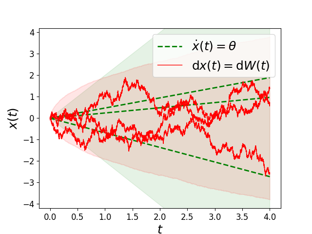
Figure 1: Visualization of sample paths and confidence intervals for the open loop system given by (4) (green) and for the reformulation presented in [3, 4, 5, 6] (red): the solutions of (4) and of (5) are distinct. The solid and dashed lines represent a handful of sample paths. The shaded regions represent the marginal $95\%$ confidence intervals.

II-C Discrete-time system

The observation we make in this note is well-known in the discrete-time problem setting. For example, starting from $x_{0}\in\mathbb{R}$, the linear system with multiplicative uncertainty

$$x_{t+1} =\theta x_{t},\quad\theta\sim\mathcal{N}(\bar{\theta},1),\quad t\in\mathbb{N},$$ (8)

is different from the system with additive disturbances

$$x_{t+1} =\bar{\theta}x_{t}+w_{k},\quad w_{k}\sim\mathcal{N}(0,1),\quad t\in\mathbb{N},$$ (9)

where the disturbances $(w_{k})_{k\in\mathbb{N}}$ are independent and identically distributed. We refer to [7, Chapter 4.7] for further discussions about this topic. We also refer to [8] for a recent analysis of systems of the form of (8) where the parameters $\theta$ are resampled at each time $t$.

III Implications and Possible Solutions

As (2) and (3) are generally not equivalent, the stability and constraint satisfaction guarantees derived for the SDE (3) in recent research [3, 4, 5, 6] do not necessarily hold for the system (2). This could yield undesired behaviors when applying such algorithms, developed on an SDE formulation of dynamics (3), to safety-critical systems where uncertainty is better modeled by (2), i.e., dynamical systems with uncertain parameters that are not changing over time.

Although (3) is not equivalent to (2), it is interesting to ask whether (3) is a conservative reformulation of (2) for the purpose of safe control. For instance, given a safe set $\mathcal{X}\subset\mathbb{R}^{n}$, if one opts to encode safety constraints through joint chance constraints of the form

$$\mathbb{P}(x(t)\in\mathcal{X}\ \forall t\in[0,T])\geq(1-\delta),$$ (10)

where $\delta\in(0,1)$ is a tolerable probability of failure, there may be settings where a controller $u$ satisfying (10) for the SDE (3) may provably satisfy (10) for the uncertain model (2). Indeed, as solutions of (3) may have unbounded total variation (as in the example presented above), which is not the case for solutions of (2), we make the conjecture that for long horizons $T$, a standard proportional-derivative-integral (PID) controller may better stabilize (2) than (3), and that similar properties hold for adaptive controllers.

Alternatively, approaches which bound the model error through the Bayesian posterior predictive variance [10] or confidence sets holding jointly over time [11, 12] exist. Given these probabilistic bounds, a policy can be synthesized yielding constraints satisfaction guarantees.

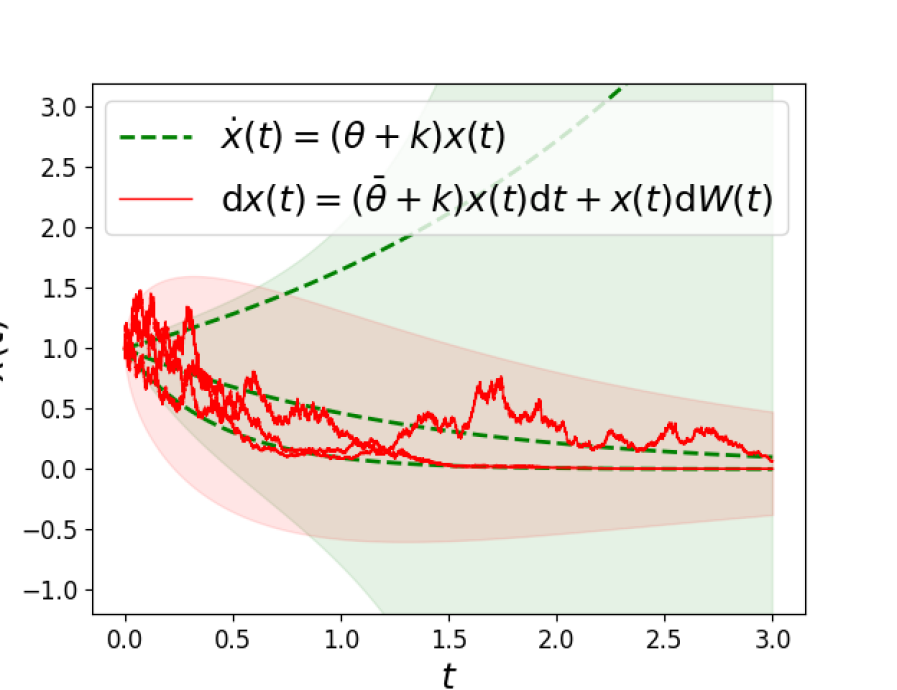
Figure 2: Visualization of sample paths and confidence intervals for the controlled system given by (6) (green) and for the reformulation presented in [3, 4, 5, 6] (red): the solutions of (6) and of (7) are distinct. The solid and dashed lines represent a handful of sample paths. The shaded regions represent the marginal $95\%$ confidence intervals.

References

- [1] C. K. Williams and C. E. Rasmussen, Gaussian processes for machine learning. MIT press, 2006.
- [2] M. A. Álvarez, L. Rosasco, and N. D. Lawrence, “Kernels for vector-valued functions: A review,” Foundations and Trends in Machine Learning, vol. 4, no. 3, pp. 195–266, 2012.
- [3] G. Chowdhary, H. A. Kingravi, J. P. How, and P. A. Vela, “Bayesian nonparametric adaptive control using Gaussian processes,” IEEE Transactions on Neural Networks, vol. 26, no. 3, pp. 537–550, 2015.
- [4] D. D. Fan, J. Nguyen, R. Thakker, N. Alatur, A. Agha-mohammadi, and E. A. Theodorou, “Bayesian learning-based adaptive control for safety critical systems,” in Proc. IEEE Conf. on Robotics and Automation, 2020.
- [5] Y. K. Nakka, A. Liu, G. Shi, A. Anandkumar, Y. Yue, and S. J. Chung, “Chance-constrained trajectory optimization for safe exploration and learning of nonlinear systems uncertainties,” IEEE Robotics and Automation Letters, vol. 1, no. 1, pp. 1–9, 2020.
- [6] G. Joshi and G. Chowdhary, “Stochastic deep model reference adaptive control,” in Proc. IEEE Conf. on Decision and Control, 2021.
- [7] A. McHutchon, “Nonlinear modelling and control using gaussian processes,” Ph.D. dissertation, University of Cambridge, 2014.
- [8] R. R. Smith and B. Bamieh, “Median, mean, and variance stability of a process under temporally correlated stochastic feedback,” IEEE Control Systems Letters, vol. 5, no. 3, 2021.
- [9] J. F. Le Gall, Brownian Motion, Martingales, and Stochastic Calculus. Springer, 2016.
- [10] M. J. Khojasteh, V. Dhiman, M. Franceschetti, and N. Atanasov, “Probabilistic safety constraints for learned high relative degree system dynamics,” in 2nd Annual Conference on Learning for Dynamics & Control, 2020.
- [11] T. Koller, F. Berkenkamp, M. Turchetta, and A. Krause, “Learning-based model predictive control for safe exploration,” in Proc. IEEE Conf. on Decision and Control, 2018.
- [12] T. Lew, A. Sharma, J. Harrison, A. Bylard, and M. Pavone, “Safe active dynamics learning and control: A sequential exploration-exploitation framework,” 2021, available at https://arxiv.org/abs/2008.11700.