Meta-learning and data augmentation for mass-generalised jet taggers

Abstract

Deep neural networks trained for jet tagging are typically specific to a narrow range of transverse momenta or jet masses. Given the large phase space that the LHC is able to probe, the potential benefit of classifiers that are effective over a wide range of masses or transverse momenta is significant. In this work we benchmark the performance of a number of methods for achieving accurate classification at masses distant from those used in training, with a focus on algorithms that leverage meta-learning. We study the discrimination of jets from boosted $Z^{\prime}$ bosons against a QCD background. We find that a simple data augmentation strategy that standardises the angular scale of jets with different masses is sufficient to produce strong generalisation. The meta-learning algorithms provide only a small improvement in generalisation when combined with this augmentation. We also comment on the relationship between mass generalisation and mass decorrelation, demonstrating that those models which generalise better than the baseline also sculpt the background to a smaller degree.

I Introduction

The introduction of deep learning techniques into collider physics in the past decade has had a significant impact upon the field. One of the main areas of application has been in the identification, or tagging, of hadronic jets at the Large Hadron Collider (LHC). Deep learning methods have been applied to heavy flavour tagging, $W$ boson and top quark tagging, quark-gluon discrimination, and the identification of the decays of new heavy resonances. Recent reviews include [1, 2, 3, 4, 5, 6, 7], and there are now numerous examples of experimental analyses using these methods [8, 9, 10, 11].

Much of this work on jet tagging studies the performance of the network within a small domain, often a relatively narrow window of jet transverse momentum, $p_{T}$, or jet mass, $m_{J}$. This means that a network trained around a specific value of $p_{T}$ or $m_{J}$ will only be highly performant in the region around those values. This specificity of the network to the statistics of the training sample is a classic limitation of neural networks [12, 13]. Given the broad range of transverse momenta and invariant masses which the LHC is capable of probing, this creates a problem for the use of machine-learning based taggers for the entirety of the available phase space.

If training data is available for the entire range over which a model will be tested, this issue can be addressed in a number of ways. A collection of neural networks can be trained, one for each window, but this requires large computational overheads and leads to discontinuities in the tagger response as domain boundaries are crossed. Alternatively, there exist domain adaptation strategies that can produce individual classifiers with near-optimal performance in the neighbourhood of the training domain. Examples include Refs. [14, 15, 16, 17, 18] as well as mass-decorrelation methods [19, 20, 21, 22, 23, 24, 25, 26, 27]. A comprehensive recent study of the performance of both data and training augmentation techniques and their implications for decorrelation is Ref. [25]. However, these approaches do not directly optimise for generalisation – that is to say, for effective tagging at $p_{T}$ or $m_{J}$ values distant from the training domain. Generalisation of this sort is useful for situations in which it is not easy to obtain sufficient training data at every desirable evaluation domain. An important example is weak or unsupervised learning on experimental data, where the data for a given process depends on the available integrated luminosity and the cross-section of the process of interest. Even in fully-supervised cases that make use of simulation, one may encounter efficiency limitations due to restrictive phase space cuts or matching requirements.

Our goal in this work is to benchmark the generalisation performance of a number of different methods. As examples of data augmentation we use planing [28, 29] and zooming [30], and for regularisation we use $L_{1}$ weight decay. We also study domain generalisation algorithms that leverage meta-learning as in Refs. [31, 32, 33, 34, 35, 36]. In contrast to the previous approaches, such algorithms directly aim to produce a model whose learning generalises to domains that are unseen during training. Specifically, we present results for the MetaReg [31] and Feature-Critic [32] algorithms.

Meta-learning is a machine learning paradigm in which part of a model’s training algorithm is itself optimised, with the goal of instilling some desired behaviour in the model across a number of related tasks [37, 38]. For a review and survey see Ref. [39]. Meta-learning can be naturally applied to a domain generalization context, where the training of a model in one domain and its evaluation in another becomes a data instance for the meta-optimisation. A successful application of meta-learned domain generalisation to jet tagging would allow future searches similar to Refs. [9, 40, 41] to train a single network instead of multiple independent networks.

We apply the different methods to the task of boosted resonance tagging across a large range of masses, focusing on the scenario where one trains a network on data at low masses and evaluates it at higher masses. This is motivated by the abundance of data at low invariant masses, while interesting new physics is likely to appear at larger masses, albeit with a small cross-section. We seek to discriminate a massive $Z^{\prime}$ vector boson from a background of QCD jets. We assume the $Z^{\prime}$ decays into light quarks, and that it is boosted so the decay products are reconstructed within a single jet. We study $Z^{\prime}$ masses between 150 and 600 GeV, dividing this range into windows separated by 50 GeV. The performance of the new algorithms is compared against a naïvely-trained baseline model. We use this resonance tagging task as an initial exploration of the concept, and discuss other possible uses in the Conclusions.

Ultimately, we find that zooming is sufficient to produce near-optimal generalisation and that the meta-learning algorithms provide only a minor advantage when used in combination with zooming. If jets are not zoomed, the meta-learning algorithms behave similarly to the baseline and $L_{1}$ regularisation is able to maintain accurate classification at new masses. In this respect our results resemble those of Ref. [25] in the context of decorrelation. They found that data augmentation using planing and another method based on principal component analysis worked as well as ML methods based on boosted decision trees and adversarial networks.

This paper is organised as follows. In Section II, we review methods for generalisation in neural networks and introduce the meta-learning strategies of Refs. [31, 32]. Sections III and IV outline the dataset generation and model implementations respectively. The classification performance of the trained models is presented in Section V. We analyse the correlations between network predictions and the input jet mass in Section VI before providing concluding remarks and comments on outlook in Section VII.

II Domain generalisation

The goal of domain generalisation is to train a model using one or more distinct domains such that its prediction accuracy generalises to unseen domains [42, 43, 44]. Implementing such an algorithm requires a collection of datasets

$$\mathcal{D}=\{D_{i}\}_{i=1}^{p}\ ,$$ (1)

where $D_{i}$ is a dataset (a set of example/label pairs) containing data in domain $i$ and there are $p$ domains available in total. In analogy to training and testing datasets, $\mathcal{D}$ is split into disjoint source and target subsets,

(3)

Data from the source domains is used to train the classifier, which is ultimately to be evaluated on data from the target domains. We will primarily be interested in the case where $\mathcal{S}$ contains jets at low masses and $\mathcal{T}$ contains jets at high masses.

In order to avoid over-fitting to the source domains one must instill some information about the relationship between domains in the training procedure. Notable approaches include data augmentation, representation learning and meta-learning. Adversarial architectures have been used in high-energy physics but typically for mass decorrelation or domain adaptation [17, 45, 25, 23]. On the other hand Ref. [44] claims that adversarial approaches excel in domain adaptation but not necessarily domain generalisation. In this work, we benchmark the generalisation performance of five methods: mass planing [28, 29], zooming [30], $L_{1}$-regularisation [46], MetaReg [31], and Feature-Critic [32]. The first two of these involve data augmentation, the third regularisation and the final two meta-learning. We go through them in turn.

II.1 Mass planing

Mass planing was one of the first methods for mass-decorrelation that was explored in ML studies of jet physics. A dataset can be mass-planed by assigning each jet in the training set a weight $w$ such that

$$w^{-1}=\frac{d\sigma_{C}}{dm_{J}}(m_{J}=m),$$ (4)

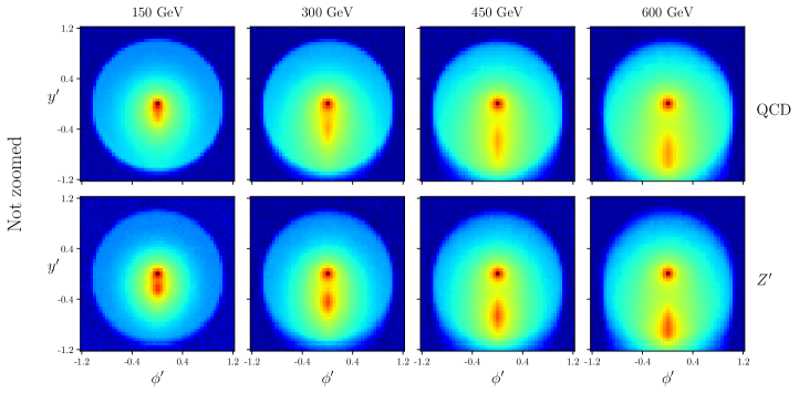
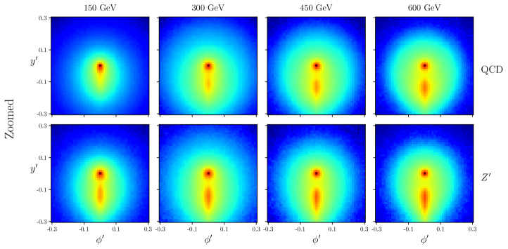
Figure 1: Average jet images of the full datasets (500K events each) preprocessed according to Section III without (top) and with (bottom) the inclusion of zooming. The background is in the first and third lines, and the signal in the second and fourth lines. Zooming standardises the signal images over as the $Z^{\prime}$ mass is varied (compare rows 2 and 4).

where $C\in\{S,B\}$ is the appropriate signal / background class label for the jet and $m$ is its mass. In practice, this simply corresponds to inverting the $m_{J}$ histogram value at the bin in which the jet lies. After such a weighting, the signal and background have uniform distributions in $m_{J}$ and as such the jet mass no longer provides discrimination.

While mass-planing is not strictly a generalisation technique, mass-decorrelation methods can in general be expected to improve performance at new masses since networks trained under these methods are discouraged from using the jet mass to make predictions. The DDT [21] method has been used for this purpose in Ref. [47].

II.2 Zooming

One way in which jets from boosted resonances with distinct masses differ is the separation of their two subjets, $\Delta R\sim 2m/p_{T}$. A neural network trained on jets in a narrow mass window does not learn this scaling relationship, leading to poor generalisation at new masses. The potential benefit of scale-invariant jet tagging has been noted in Refs. [30, 48, 21], motivating the addition of a zooming transformation to the jet preprocessing steps.

The implementation in Ref. [30] reclusters the jet into subjets and then scales their separation by a factor dependent on the jet mass and transverse momentum. For application to widely-varying jet masses, we use a different procedure in which no reference to $m_{J}$, jet $p_{T}$ or clustering radius is used. Specifically, we scale the $\eta$ and $\phi$ coordinates of all jet constituents by a factor that ensures the average distance between each particle and the leading constituent is 0.1. We find that this variant of zooming is effective, demonstrated by the averaged jet images for our datasets shown in Fig. 1. The top two rows show the background and signal images without zooming, and the bottom two are the images after zooming has been applied. Comparing the second and fourth rows, the zooming procedure standardises the signal images over a range of $Z^{\prime}$ masses.

II.3 Regularisation

Regularisation may be defined as any modification to a learning algorithm that reduces generalisation error, even at the expense of increased training error. In this class, the most common techniques used in modern neural networks include weight decay ($L_{1}$ or $L_{2}$ regularisation [46]), Batch Normalisation [49], Dropout [50] and DropConnect [51]. While these methods lead to improved generalisation error for testing samples drawn from the same distribution as the training data, they are not necessarily effective at domain generalisation.

In this work, we implement $L_{1}$ regularisation, where the classification loss $\mathcal{L}$ is extended as

$$\mathcal{L}\rightarrow\mathcal{L}+\lambda\sum_{i}\left|\theta_{i}\right|,$$ (5)

where $\theta_{i}$ are the neural network weights and $\lambda$ is a hyperparameter that sets the regularisation strength. One can similarly define $L_{2}$ regularisation by

$$\mathcal{L}\rightarrow\mathcal{L}+\lambda\sum_{i}{\theta_{i}}^{2}.$$ (6)

Gradient updates derived from these losses include a term that reduces the size of the weights $\theta$, thus mitigating specificity and, thereby, overfitting. The difference between the $L_{1}$ and $L_{2}$ schemes is that the former allows weights to be sent to zero while the contributions to the gradient from the latter are proportional to the size of the weight, which damps the decay. We have also implemented and studied the generalisation behaviour of $L_{2}$ regularisation. However, we find that for the task we study $L_{2}$ regularisation does not generalise as well as $L_{1}$, and so we only present results for $L_{1}$ regularisation.

II.4 Meta-learning

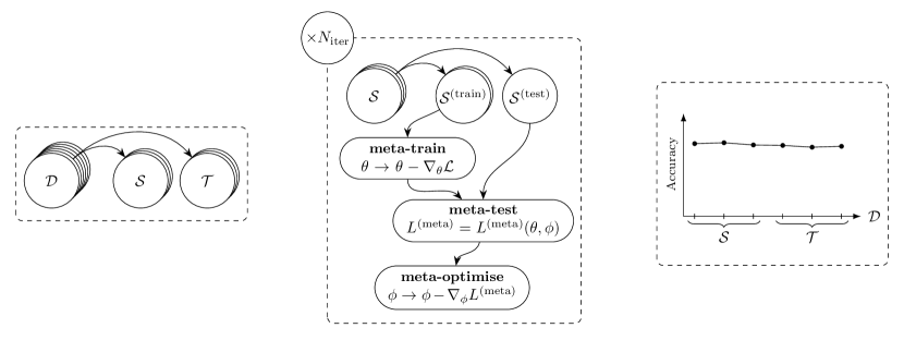
Figure 2: General schematic for domain generalisation via meta-learning. A collection of datasets $\mathcal{D}$ spread across the domain is split into source and target collections. The parameters $\phi$ of the meta-representation are updated using data from the source domains only. A particular algorithm conducts meta-training, meta-testing, and meta-optimisation at each iteration. Finally, the model is evaluated on the entire collection $\mathcal{D}$ and the degree of generalisation achieved can be measured.

Meta-learning is a machine learning paradigm in which a model’s training algorithm is itself optimised, typically to achieve some goal over a number of related tasks. For domain generalisation, the tasks differ only by shifts in the given domain and the goal is to improve performance on unseen domains.

The general prescription for meta-learning is as follows. One first parametrises a component of the base model’s training algorithm by some variables $\phi$. This component is referred to as the meta-representation and can take a variety of forms such as the initial network weights [38, 33], the loss function [32], the optimiser [52], a regulariser [31] or even the model architecture itself. For a more exhaustive categorisation, see Ref. [39]. The parameters of the meta-representation are updated iteratively, with each step divided into three stages: meta-training, meta-testing and meta-optimisation. During meta-training, the base classifier is updated via gradient descent using the meta-representation variables $\phi$. The model is then evaluated in the meta-test stage by calculating a meta-loss $L^{(\mathrm{meta})}$ that encapsulates the meta-learning objective. Since $L^{(\mathrm{meta})}$ depends on the parameters $\phi$ through the meta-train phase, back-propagation can be used to find a direction $d\phi$ that gives improved performance with respect to the goal. The variables $\phi$ are updated in this direction during meta-optimisation.

Fig. 2 illustrates how meta-learning operates in a domain generalisation context. In this case, meta-training and meta-testing are conducted in disjoint subsets of the source domains, denoted $\mathcal{S}^{(\mathrm{train})}$ and $\mathcal{S}^{(\mathrm{test})}$ respectively. In this way, source/target domain shift is simulated as the model is trained. By taking the meta-loss to be the classification loss of the model on $\mathcal{S}^{(\mathrm{test})}$, the meta-representation parameters $\phi$ are optimised to enforce robust performance in unseen domains. The representation can then be deployed on a new model to be trained on all source domains, and is expected to achieve improved performance on the target domains compared with a model trained in a naïve fashion.

Below, we introduce the two meta-learning algorithms that we benchmark in this work: MetaReg [31] for which the meta-representation is a weight regulariser and Feature-Critic [32] for which the meta-representation is an auxiliary loss function that depends on the latent-space features produced by the model. We also implemented the MLDG algorithm [33], which meta-learns the network’s weight initialisation, but found no difference in performance compared to the baseline. Accordingly we do not include results for MLDG in our plots. Other examples of domain generalisation via meta-learning that could also be applied include Refs. [34, 35, 36].

Meta-Regularisation

The MetaReg [31] algorithm uses a regulariser $R_{\phi}$ as the meta-representation. In Ref. [31] three parametrised regularisers were used: weighted $L_{1}$ and $L_{2}$ (in which the sums in Equations 5 and 6 are weighted by the learned parameters $\phi$) and a multi-layer perceptron (MLP).

To avoid memory limitations for large models (tracking higher-order gradients through many updates is costly) the learned regulariser acts only on a subset of the network layers. As such the base model is split into two subnetworks: the feature extractor $F_{\psi}$ and the task network $T_{\theta}$. The full network is the composition $T_{\theta}\circ F_{\psi}$ and regularization is only applied to task network weights $\theta$. During optimisation of the regulariser, a single feature extractor is updated from all source domains, while independent task networks are used in each domain. In this way, only the task networks learn domain-specific information and this is what allows the regulariser to enforce domain invariance.

Training the meta-regulariser proceeds by randomly initialising weights $\phi$, $\psi$ and $\theta_{i}$ for the regulariser, feature extractor and $i$^th task network respectively, before performing the following steps at each iteration.

1. In each source domain $D_{i}$, perform $k$ updates of the network $T_{i}\circ F$ without regularisation:

   $$\left.\begin{matrix}\psi\rightarrow\psi-\alpha\nabla_{\psi}\mathcal{L}^{(i)}_{\psi,\theta_{i}}\\[8.0pt] \theta_{i}\rightarrow\theta_{i}-\alpha\nabla_{\theta_{i}}\mathcal{L}^{(i)}_{\psi,\theta_{i}}\end{matrix}\ \right\}\times k\,.$$

   where $\mathcal{L}^{(i)}_{\psi,\theta}=\mathcal{L}(y,T_{\theta_{i}}\circ F_{\psi}({\bf x}))$ is the classification loss of the model evaluated on ${\bf x},\,y\sim D_{i}$.

2. Randomly select $a,b\in\{1,\>\cdots,p\}$ (where $p$ is the number of domains) such that $a\neq b$ and initialize a new task network $\hat{T}$ with parameters $\theta_{a}$:

   $$\hat{\theta}\rightarrow\theta_{a}\,.$$

3. Meta-train on $D_{a}$ by performing $l$ updates to $\hat{\theta}$ for the network $\hat{T}\circ F$ using the regularised loss:

   $$\left.\begin{matrix}\hat{\theta}\rightarrow\hat{\theta}-\alpha\nabla_{\hat{\theta}}\left(\mathcal{L}^{(a)}_{\psi,\hat{\theta}}+R_{\phi}(\hat{\theta})\right)\end{matrix}\ \right\}\times l\,.$$

4. Meta-test by calculating the unregularised loss on $D_{b}$ using $\psi$ and $\hat{\theta}$:

   $$L^{(\mathrm{meta})}=\mathcal{L}^{(b)}_{\psi,\hat{\theta}}$$

5. Meta-optimise by updating the regulariser parameters using the meta-test loss:

   $$\phi\rightarrow\phi-\beta\nabla_{\phi}L^{(\mathrm{meta})}\,.$$

In the above, $\alpha$ and $\beta$ are learning rates. Once the specified number of meta-optimisation steps has been completed, the regulariser weights $\phi$ are frozen. A new model is then initialised using the trained feature extractor and random task network. The model is then trained to minimise the regularised loss using any optimisation algorithm.

Feature-Critic

The Feature-Critic algorithm was introduced in Ref. [32], which addresses the heterogeneous domain generalisation problem wherein the label spaces are not shared between domains. It is compatible, however, with the more common homogeneous case that we explore here.

This algorithm learns a contribution to the loss function that aims to promote cross-domain performance and, similarly to MetaReg, it considers the model separated into a feature extractor, $F_{\psi}$ and a task network $T_{\theta}$. The meta-representation is a feature critic denoted $h_{\phi}$ which acts on the features produced by $F$. The critic is trained alongside the feature extractor and task network in the following way before its parameters are frozen and the full model is fine-tuned.

1. Randomly split $\mathcal{S}$ into $\mathcal{S}^{(\mathrm{train})}$ and $\mathcal{S}^{(\mathrm{test})}$ in the same fashion as Eq. 3, ensuring $\mathcal{S}^{(\mathrm{train})}$ contains $S$ domains.

2. Meta-train by calculating classification and auxiliary losses on $\mathcal{S}^{(\mathrm{train})}$ and defining updated weights:

   $${\bf x},\,y\sim\mathcal{S}^{(\mathrm{train})}$$

   $$\psi_{\mathrm{old}}=\psi-\gamma\nabla_{\psi}\mathcal{L}^{(\mathrm{train})}_{\psi,\theta}$$

   $$\psi_{\mathrm{new}}=\psi_{\mathrm{old}}-\gamma\nabla_{\psi}h_{\phi}(F_{\psi}({\bf x}))\,.$$

3. Meta-test by sampling $\mathcal{S}^{(\mathrm{test})}$ and calculating the improvement in classification provided by the critic,

   $$L^{(\mathrm{meta})}=\tanh\left(\mathcal{L}^{(\mathrm{test})}_{\psi_{\mathrm{new}},\theta}-\mathcal{L}^{(\mathrm{test})}_{\psi_{\mathrm{old}},\theta}\right)\,.$$

4. Meta-optimise by updating the critic parameters. The feature extractor and task network are also updated here:

   $$\psi\rightarrow\psi-\alpha\nabla_{\psi}\left(\mathcal{L}^{(\mathrm{train})}_{\psi,\theta}+h_{\phi}(F_{\psi}({\bf x}))\right)$$

   $$\theta\rightarrow\theta-\alpha\nabla_{\theta}\left(\mathcal{L}^{(\mathrm{train})}_{\psi,\theta}+h_{\phi}(F_{\psi}({\bf x}))\right)$$

   $$\phi\rightarrow\phi-\beta\nabla_{\phi}L^{(\mathrm{meta})}\,.$$

In the above algorithm, $\alpha$, $\beta$ and $\gamma$ are learning rates.

III Simulation details

In this work, we train networks to discriminate signal jets produced by a boosted hypothetical $Z^{\prime}$ boson which decays into a pair of light quarks, against a QCD jet background. We consider a range of potential resonance masses $m_{Z^{\prime}}$. We focus on a relatively light (sub-TeV), boosted $Z^{\prime}$ whose origin may be in the decay of a heavier multi-TeV resonance. Accordingly, we are interested in the situation where the decay products from the $Z^{\prime}$ decay are reconstructed within the same large radius jet.

To generate the datasets, signal and background processes are simulated with MadGraph5 2.8.0 [53], showered in Pythia 8.244 [54] then passed to Delphes 3.4.2 [55] with the default CMS card. For the signal, we use a simple $Z^{\prime}$ model from FeynRules [56]. The signal and background jets are obtained from $pp\to Z(\nu\bar{\nu})Z^{\prime}$ and $pp\to Z(\nu\bar{\nu})j$ processes respectively. We produce 10 datasets, corresponding to masses $m_{Z^{\prime}}=150$ GeV to $m_{Z^{\prime}}=600$ GeV at $50$ GeV intervals, each of which contains $5\times 10^{5}$ $Z^{\prime}$ and $5\times 10^{5}$ QCD events. Thus the full collection of datasets is $\mathcal{D}=\{D_{150},D_{200},\>\cdots,D_{600}\}$ where the labels indicate the $Z^{\prime}$ mass. The $Z^{\prime}$ widths are calculated automatically by MadGraph, which with the default couplings gives $\Gamma_{Z^{\prime}}/m_{Z^{\prime}}\sim 0.0275$ at every mass.

Within Delphes, events are clustered by FastJet 3.3.4 using the anti-$k_{t}$ algorithm with $R=1.0$ and the leading jet is selected. Parton-level cuts of $|\eta_{J}|,|\eta_{Z^{\prime}}|<2.0$ and $\not\!\!E_{T}>1.2$ TeV are applied in MadGraph, the latter of which boosts the jets to ensure that decay products from the $Z^{\prime}$ fall within a cone of appropriate radius for jet reconstruction. This is motivated by simplicity and experimental searches, which usually do not vary the jet radius. Since this missing energy cut is the same for all datasets, jets in different datasets will have different boosts, which may be considered a component of the domain shift which our networks will learn to generalise. Cuts of $|m_{J}-m_{Z^{\prime}}|<m_{Z^{\prime}}/4$ and $p_{T}>1.2$ TeV are applied after detector simulation. The size of the jet mass window varies to account for the scaling of the ${Z^{\prime}}$ width with its mass. This causes overlaps between nearby domains which results in a jagged QCD jet mass distribution for aggregated datasets. Although this can be resolved by an appropriate reweighting of events that takes into account both the number of mass windows in which a jet lies as well as the relative cross-section between windows, such a reweighting increases domain specificity so we do not explore it here.

Jets are preprocessed by first translating all constituents in the rapidity-azimuth plane such that the leading constituent lies at the origin. A rotation is then applied to position the centre of momentum below the origin. Jets are then optionally zoomed as per Section II.2. Each jet is stored as a list of constituent information in the format $(p_{T}/p_{T,J},\eta^{\prime},\phi^{\prime},g(\text{{pdg\_id}}))$ where $\eta^{\prime}$ and $\phi^{\prime}$ respectively denote pseudorapidity and azimuthal angle coordinates after the mentioned transformations and $g$ maps Particle Data Group Monte Carlo numbers to small floats beginning at $0.05$ and incrementing $0.1$ for each class of constituent. The arrays are serialised and saved in TFRecord format allowing for efficient interfacing with Tensorflow [57], which is necessary to avoid memory issues associated with loading a large number of datasets. In order to facilitate future studies on mass generalisation, the complete collection of datasets has been made available at Ref. [58].

IV Model details

Hyperparameter	MetaReg	Feature-Critic
Iterations	$10^{\,3}$, $\bm{5\times 10^{\,3}}$, $10^{\,4}$, $5\times 10^{\,4}$	$10^{\,3}$, $5\times 10^{\,3}$, $\bm{10^{\,4}}$, $5\times 10^{\,4}$
$\beta$	$10^{-1}$, $10^{-2}$, $\bm{10^{-3}}$, $10^{-4}$, $10^{-5}$, $10^{-6}$	$10^{-1}$, $10^{-2}$, $\bm{10^{-3}}$, $10^{-4}$, $10^{-5}$, $10^{-6}$
Regulariser	Weighted $\bm{L_{1}}$, Weighted $L_{2}$, MLP	-
$k$	1, $\bm{4}$, 16, 32	-
$l$	$\bm{1}$, 4, 8, 16	-
$\gamma$	-	$10^{-1}$, $10^{-2}$, $10^{-3}$, $10^{-4}$, $\bm{10^{-5}}$, $10^{-6}$
$S$	-	$\bm{1}$, 2

Table 1: A summary of the hyperparameters for MetaReg and Feature-Critic that were explored by grid search. Selected parameters are shown in bold. The learning rate hyperparameter $\alpha$ is fixed to $10^{-3}$ to match the baseline.

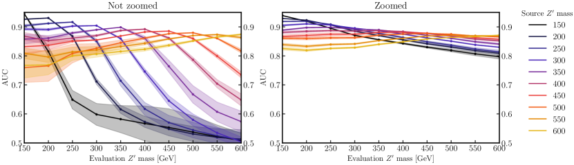
Figure 3: The performance of baseline PFNs trained on single datasets with (right) and without (left) zooming. Zooming improves generalisation for all source masses, particularly for networks trained at low masses which generalise to high masses. Curves are the mean of 5 independent networks with bands displaying one standard deviation around the mean.

We will compare the performance of the approaches from Section II using a Particle Flow Network (PFN) [59] as the underlying classifier. PFNs are an implementation of the DeepSets [60] framework and treat jets as point clouds, where each point is a jet constituent. Each particle in the jet is mapped into a latent space with a per-particle network. The outputs of these networks are then summed over to obtain a latent representation of the whole jet, which is then mapped by another jet-level network to an output giving the value of the learned observable. For all algorithms we study, the PFN has a per-particle network with layer sizes (100,100,256) and a jet-level network with layer sizes (100,100,100,2). All parameters use Glorot uniform initialisation [61] and all activations are rectified linear units (ReLU) except for the two-unit output layer for which we which we use a softmax function.

For training the PFNs, we use the cross-entropy classification loss optimised via AMSGrad [62] with learning rate $\alpha=10^{-3}$ and a mini-batch size of 200. For $L_{1}$-regularised training, we use a weight of $10^{-3}$ and the penalty applies only to the jet-level network. Weights for mass planing are calculated from a 64-bin histogram and normalised to have unit mean per batch. With the exception of the meta-learning algorithms, which consume data from different source domains as outlined in Section II.4, the networks are fit on all source domains as a single aggregated dataset. We also trained PFNs on each domain individually with the same settings. In all cases, we use a training/validation/testing split of 0.75/0.1/0.15 and the PFN is trained for a maximum of 100 epochs. If the validation loss has not decreased for 5 epochs, training is halted and the best weights are restored.

We implement the MetaReg and Feature-Critic algorithms in TensorFlow and fix their $\alpha$ learning rates to $10^{-3}$ to match the baseline PFN. In both algorithms, the feature extractor $F_{\psi}$ is taken to be the per-particle network (including the latent-space sum) and the task network $T_{\theta}$ is the jet-level network. For Feature-Critic, the auxiliary loss $h_{\phi}$ has two hidden layers with 512 and 128 nodes with ReLU activations. The scalar outputs of $h_{\phi}$ and the MetaReg regulariser $R_{\phi}$ are passed through a softplus function to ensure a convex loss. While no such activation is applied to $R_{\phi}$ in Ref. [31], without it the loss function is unbounded from below resulting in unstable training. Meta-optimisation is performed using AMSGrad and the remaining hyperparameters are selected via a grid search on $\mathcal{S}=\{D_{150},D_{200},D_{250}\}$ with zooming which we summarise in Table 1. We adopt those parameters that produce the greatest AUC score on $D_{300}$.

V Results and Discussion

In this Section, we present the performance of the trained models under various generalisation settings. Firstly, we demonstrate the benefit of zooming jets in Fig. 3, which shows the AUC scores of PFNs trained with baseline settings on an individual source domain without (left panel) and with zooming (right panel). In the left panel we see that the performance of each network degrades substantially away from the domain in which it was trained. A network trained in the $m_{Z^{\prime}}=150$ GeV domain is only slightly better than a random classifier at 600 GeV. The maximum AUC achieved at each mass decreases at larger masses due to the fact that high mass QCD jets have stronger pronged structure and thus the discrimination task is inherently more difficult in these datasets.

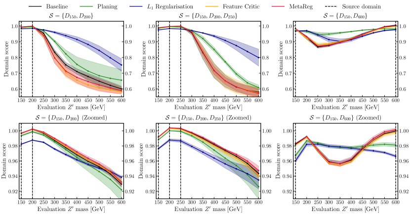
Figure 4: Domain scores for each of the trained models on various source/target splits. Source domains are indicated by vertical dashed lines. The top row shows results without zooming and the bottom row shows results with zooming (note the change in vertical scale between rows). Curves are the mean of 5 independent networks with bands displaying one standard deviation around the mean.

From the right panel we see that each of the performance curves is much flatter as the domain varies. The inclusion of zooming in the preprocessing steps significantly improves the generalisation performance of all models. This indicates that the difference in angular scale between jets of different masses is a large hindrance to the neural networks’ capability to generalise. However, it remains the case that each model provides poorer classification when evaluated away from the source dataset. This is not surprising; variation in the scale of the jets is only a component of the domain shift, and other factors such as different charged particle multiplicity (for instance) will also matter.

Next, we present results for models trained on multiple source domains. Fig. 4 contains plots of the models’ performance in the test split of all datasets. Each curve is the mean of the AUC scores of five models normalised domain-wise by the AUC of a baseline PFN trained only on the corresponding dataset (the peaks in Fig. 3). We call this metric the domain score and in these terms, a perfectly general model produces a flat line at 1. The bands around the curves show one standard deviation around the mean. The top and bottom rows of the figure are results without and with zooming respectively, and the columns correspond to different source masses, which are shown in each panel by the vertical dashed lines.

Focusing on the top row, where jets are not zoomed, we see that both meta-learning algorithms exhibit near-baseline performance for $\mathcal{S}=\{D_{150},D_{200}\}$ and $\mathcal{S}=\{D_{150},D_{200},D_{250}\}$, while the $L_{1}$-regularised model achieves vastly improved generalisation at the cost of slightly poorer classification on the source masses. The mass-planed network performs somewhat better than the baseline in these cases, but is the best at interpolating between distant source domains as in $\mathcal{S}=\{D_{150},D_{600}\}$. The $L_{1}$ regulariser also bridges the gap better than the baseline.

The results are different when zooming is applied to the jets. In this case, all models including the baseline maintain domain scores above 0.9 at all masses (note the change in scale of the vertical axis compared to the top row). For $S=\{D_{150},D_{200}\}$ in the bottom-left panel, the meta-learning algorithms and the baseline slightly outperform the other classifiers, with the $L_{1}$ regularized model being the worst classifier at low masses. At high masses all the classifiers achieve domain scores which are equivalent within the uncertainty bands, although planing generalises least well.

When another source dataset is added, as in $\mathcal{S}=\{D_{150},D_{200},D_{250}\}$ in the bottom centre panel, the results are similar. Finally, when the source domains are chosen at the extremities so that $\mathcal{S}=\{D_{150},D_{600}\}$, mass-planing exhibits the most uniform performance across all the domains. However, the meta-learning algorithms and the baseline have higher domain scores in the vicinity of the source domains but generalise less well.

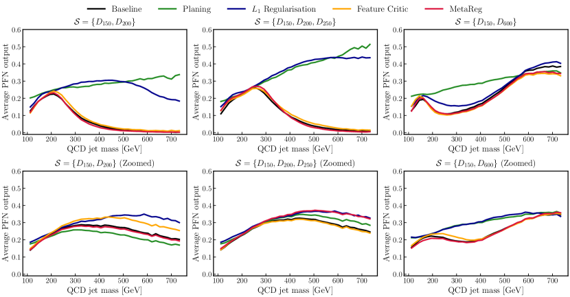
Figure 5: Average PFN output for QCD jets across all masses. Results are shown with (bottom row) and without (top row) zooming. The averages are over jets in the testing splits of all datasets for 5 independent networks.

Zooming improves the generalisation of all models. This indicates that the regularisation and meta-learning methods are unable to completely account for the variation of jets’ angular scales at different masses (or else zooming would not affect their performance). There is also other information that is not being fully used by the networks. This is clear from decrease in performance of the zoomed networks away from the domains where they were trained. The particle multiplicity in a jet is an example of such information not captured in the jet angular distribution. Our results show that the meta-learning models are not optimally leveraging this information relative to the PFN baseline. While some improvement over the baseline is achieved when only two source masses are used, the magnitude of this improvement is small compared to the computational overhead of the meta-learning algorithms.

Given the success of zooming, an alternative approach would be to consider scale transformations as a symmetry of the data and embed this information into the network architecture itself. There already exists work on jet taggers that are equivariant to other symmetries of jets [65, 66, 67, 68] as well as implementations of scaling-equivariant CNNs [69, 70, 71]. Of course, in applications where the relationship between domains is less easily understood, it may not be possible to identify the appropriate data augmentation procedure. Our results suggest that in such a scenario, simple weight regularisation is able to partially resolve this gap. Alternatively, one can attempt to learn the transformations as in Ref. [72].

The fact that MetaReg is often outperformed by standard $L_{1}$ regularisation indicates that it is not able to find the optimal regulariser in those cases. There are a number of potential reasons for this, for example the algorithm may be particularly sensitive to the hyperparameters that we matched to the baseline (the learning rate $\alpha$ and the batch size). It may be possible to improve the performance of MetaReg with a more thorough grid search that includes the full space of hyperparameters, including the MLP regulariser architecture. However, such a process is computationally expensive and is not guaranteed to improve on the far simpler $L_{1}$ regularisation.

VI Correlation with jet mass

The performance of mass-planing in Fig. 4 demonstrates that mass-generalisation is not necessarily a byproduct of decorrelation. In this section, we pose the reverse question: do generalised models automatically exhibit less correlation with the jet mass than the baseline? To answer this question, we plot the average prediction score output by the different PFNs when evaluated on QCD jets across all datasets. In such a way, networks that are correlated with the jet mass can be identified by the presence of a peak in the region of the source masses. This peak is what leads to a background sculpting effect which makes the estimation of systematic uncertainties difficult, since a fixed selection threshold that intersects the peak will prefer jets within the peak. In contrast, a network that is not correlated with mass will produce a flat curve.

Fig. 5 presents such plots for different source masses with and without zooming the jets. The best decorrelation is achieved by the mass-planed PFN as expected. When jets are not zoomed, the two meta-learning algorithms behave essentially the same as the baseline, exhibiting a strong peak at the source masses. However, the $L_{1}$-regularized PFN is noticeably decorrelated compared to the baseline. This is interesting given that there is no special treatment of the jet mass in this approach, only a generic penalty for large weights in the network.

When jets are zoomed all models behave similarly, with far less correlation than the unzoomed baseline. In this case, we only observe a difference between the baseline and mass-planing for $\mathcal{S}=\{D_{150},D_{600}\}$. In combination with the results of the previous section, this suggests that decorrelation from the jet mass is indeed delivered as a byproduct of effective generalisation. Specifically, the $L_{1}$-regularised PFN is the most general model on $\mathcal{S}=\{D_{150},D_{200}\}$ and $\mathcal{S}=\{D_{150},D_{200},D_{250}\}$ where it is also the least correlated. Similarly, zooming provides strong generalisation for all models and also leads to relatively small dependence on jet mass.

VII Conclusions

Jet-tagging has become an important area for the application of machine-learning methods at the Large Hadron Collider. Studies have often been carried out in narrow ranges of transverse momentum or invariant mass, raising the question of what is the optimum way to apply these methods over the full kinematic range available.

In the context of boosted boson tagging at a wide range of masses, we have studied the interplay between regularisation, mass decorrelation, preprocessing, and domain generalisation algorithms. Among the existing techniques we used were $L_{1}$ regularisation, planing and zooming, where the zooming procedure was varied to be independent of the mass, $p_{T}$ or clustering radius of the jet. We also studied two domain generalisation algorithms based on meta-learning, namely the MetaReg and Feature-Critic algorithms.

We found that zooming alone is enough to yield strong generalisation. The meta-learning algorithms only lead to improvement over the baseline when used in combination with zooming. However, this improvement was minor and limited to settings with minimal training masses. In the absence of zooming, $L_{1}$ regularisation lead to the best generalisation. Mass-decorrelation via planing was most effective at generalising between distant training points.

We have also investigated the correlation with the jet mass of the model predictions trained under each method. When jets were not zoomed, $L_{1}$ regularisation led to similar or improved decorrelation from the jet mass compared to planing despite being ignorant to jet masses. When zooming was included in the preprocessing steps, all models exhibited relatively little correlation with jet mass.

While the MetaReg and Feature-Critic displayed limited utility, one could also study the efficacy of other learning algorithms such as Refs. [34, 35, 36] based on meta-learning, domain-invariant variational auto-encoders [73], representation learning [72] or scale-equivariant networks [69, 70, 71]. There is also recent work on ‘stable’ learning which takes a different approach to generalising to unseen domains [74, 75].

The techniques explored here are also applicable to alternate scenarios wherein a different property of the signal varies across a range. An example case is resonant/non-resonant dijet classification which could be generalised across $m_{JJ}$. It may also be possible to explore discrete domains such as the choice of Monte Carlo event generator, where generalisation would correspond to learning only generator-non-specific information, with applications to experimental data, motivated by Ref. [30]. One could also consider the possibility of unsupervised domain-generalisation, for instance via the transfer-learning method in Ref. [76] where no label information is present in the source domain.

References

- Larkoski et al. [2020] A. J. Larkoski, I. Moult, and B. Nachman, Phys. Rept. 841, 1 (2020), arXiv:1709.04464 [hep-ph] .
- Guest et al. [2018] D. Guest, K. Cranmer, and D. Whiteson, Ann. Rev. Nucl. Part. Sci. 68, 161 (2018), arXiv:1806.11484 [hep-ex] .
- Albertsson et al. [2018] K. Albertsson et al., J. Phys. Conf. Ser. 1085, 022008 (2018), arXiv:1807.02876 [physics.comp-ph] .
- Radovic et al. [2018] A. Radovic, M. Williams, D. Rousseau, M. Kagan, D. Bonacorsi, A. Himmel, A. Aurisano, K. Terao, and T. Wongjirad, Nature 560, 41 (2018).
- Carleo et al. [2019] G. Carleo, I. Cirac, K. Cranmer, L. Daudet, M. Schuld, N. Tishby, L. Vogt-Maranto, and L. Zdeborová, Rev. Mod. Phys. 91, 045002 (2019), arXiv:1903.10563 [physics.comp-ph] .
- Bourilkov [2020] D. Bourilkov, Int. J. Mod. Phys. A 34, 1930019 (2020), arXiv:1912.08245 [physics.data-an] .
- Schwartz [2021] M. D. Schwartz, HDSR 10.1162/99608f92.beeb1183 (2021).
- Sirunyan et al. [2020a] A. M. Sirunyan et al. (CMS), J. High Energy Phys. 12 (2020), 85, arXiv:2006.13251 [hep-ex] .
- Aad et al. [2020a] G. Aad et al. (ATLAS), Phys. Rev. Lett. 125, 131801 (2020a), arXiv:2005.02983 [hep-ex] .
- Aad et al. [2020b] G. Aad et al. (ATLAS), Phys. Rev. Lett. 125, 221802 (2020b), arXiv:2004.01678 [hep-ex] .
- Aad et al. [2020c] G. Aad et al. (ATLAS), Phys. Lett. B 801, 135145 (2020c), arXiv:1908.06765 [hep-ex] .
- Sugiyama and Storkey [2007] M. Sugiyama and A. J. Storkey, in NeurIPS, Vol. 19 (MIT Press, 2007) pp. 1337–1344.
- Torralba and Efros [2011] A. Torralba and A. A. Efros, in CVPR 2011 (2011) pp. 1521–1528.
- Baldi et al. [2016] P. Baldi, K. Cranmer, T. Faucett, P. Sadowski, and D. Whiteson, Eur. Phys. J. C 76, 235 (2016), arXiv:1601.07913 [hep-ex] .
- Shimmin et al. [2017] C. Shimmin, P. Sadowski, P. Baldi, E. Weik, D. Whiteson, E. Goul, and A. Søgaard, Phys. Rev. D 96, 074034 (2017), arXiv:1703.03507 [hep-ex] .
- Aguilar-Saavedra et al. [2021] J. A. Aguilar-Saavedra, F. R. Joaquim, and J. F. Seabra, J. High Energy Phys. 03 (2021), 012, arXiv:2008.12792 [hep-ph] .
- Louppe et al. [2017] G. Louppe, M. Kagan, and K. Cranmer, in NeurIPS, Vol. 30 (Curran Associates, Inc., 2017).
- Aguilar-Saavedra [2021] J. A. Aguilar-Saavedra, Anomaly detection from mass unspecific jet tagging (2021), arXiv:2111.02647 [hep-ph] .
- Stevens and Williams [2013] J. Stevens and M. Williams, J. Instrum. 8 (12), P12013, arXiv:1305.7248 [nucl-ex] .
- Rogozhnikov et al. [2015] A. Rogozhnikov, A. Bukva, V. V. Gligorov, A. Ustyuzhanin, and M. Williams, J. Instrum. 10 (03), T03002, arXiv:1410.4140 [hep-ex] .
- Dolen et al. [2016] J. Dolen, P. Harris, S. Marzani, S. Rappoccio, and N. Tran, J. High Energy Phys. 5 (2016), 156, arXiv:1603.00027 [hep-ph] .
- Moult et al. [2018] I. Moult, B. Nachman, and D. Neill, J. High Energy Phys. 05 (2018), 2, arXiv:1710.06859 [hep-ph] .
- Heimel et al. [2019] T. Heimel, G. Kasieczka, T. Plehn, and J. M. Thompson, SciPost Phys. 6, 030 (2019), arXiv:1808.08979 [hep-ph] .
- Englert et al. [2019] C. Englert, P. Galler, P. Harris, and M. Spannowsky, Eur. Phys. J. C 79, 4 (2019), arXiv:1807.08763 [hep-ph] .
- Bradshaw et al. [2020] L. Bradshaw, R. K. Mishra, A. Mitridate, and B. Ostdiek, SciPost Phys. 8, 011 (2020), arXiv:1908.08959 [hep-ph] .
- Kitouni et al. [2020] O. Kitouni, B. Nachman, C. Weisser, and M. Williams, J. High Energy Phys. 04 (2021), 70, arXiv:2010.09745 [hep-ph] .
- Kasieczka and Shih [2020] G. Kasieczka and D. Shih, Phys. Rev. Lett. 125, 122001 (2020), arXiv:2001.05310 [hep-ph] .
- de Oliveira et al. [2016] L. de Oliveira, M. Kagan, L. Mackey, B. Nachman, and A. Schwartzman, J. High Energy Phys. 07 (2016), 69, arXiv:1511.05190 [hep-ph] .
- Chang et al. [2018] S. Chang, T. Cohen, and B. Ostdiek, Phys. Rev. D 97, 056009 (2018), arXiv:1709.10106 [hep-ph] .
- Barnard et al. [2017] J. Barnard, E. N. Dawe, M. J. Dolan, and N. Rajcic, Phys. Rev. D 95, 014018 (2017), arXiv:1609.00607 [hep-ph] .
- Balaji et al. [2018] Y. Balaji, S. Sankaranarayanan, and R. Chellappa, in NeurIPS, Vol. 31 (Curran Associates, Inc., 2018).
- Li et al. [2019] Y. Li, Y. Yang, W. Zhou, and T. Hospedales, in ICML, Vol. 97 (PMLR, 2019) pp. 3915–3924.
- Li et al. [2018] D. Li, Y. Yang, Y.-Z. Song, and T. M. Hospedales, in AAAI (2018) arXiv:1710.03463 [cs.LG] .
- Dou et al. [2019] Q. Dou, D. C. de Castro, K. Kamnitsas, and B. Glocker, CoRR (2019), 1910.13580 [cs.CV] .
- Chen et al. [2020] K. Chen, D. Zhuang, and J. M. Chang, CoRR (2020), 2011.00444 [cs.LG] .
- Du et al. [2020] Y. Du, J. Xu, H. Xiong, Q. Qiu, X. Zhen, C. G. M. Snoek, and L. Shao, CoRR (2020), 2007.07645 [cs.CV] .
- Thrun and Pratt [1998] S. Thrun and L. Pratt, eds., Learning to Learn (Kluwer Academic Publishers, USA, 1998).
- Finn et al. [2017] C. Finn, P. Abbeel, and S. Levine, CoRR (2017), 1703.03400 [cs.LG] .
- Hospedales et al. [2020] T. M. Hospedales, A. Antoniou, P. Micaelli, and A. J. Storkey, CoRR (2020), 2004.05439 [cs.LG] .
- Chatrchyan et al. [2012] S. Chatrchyan et al. (CMS), Phys. Lett. B 710, 26 (2012), arXiv:1202.1488 [hep-ex] .
- Aaltonen et al. [2012] T. Aaltonen et al. (CDF, D0), Phys. Rev. Lett. 109, 071804 (2012), arXiv:1207.6436 [hep-ex] .
- Blanchard et al. [2011] G. Blanchard, G. Lee, and C. Scott, in NeurIPS, Vol. 24 (Curran Associates, Inc., 2011).
- Zhou et al. [2021] K. Zhou, Z. Liu, Y. Qiao, T. Xiang, and C. C. Loy, CoRR (2021), arXiv:2103.02503 [cs.LG] .
- Wang et al. [2021] J. Wang, C. Lan, C. Liu, Y. Ouyang, and T. Qin, CoRR (2021), 2103.03097 [cs.LG] .
- Clavijo et al. [2020] J. M. Clavijo, P. Glaysher, and J. M. Katzy, Adversarial domain adaptation to reduce sample bias of a high energy physics classifier (2020), arXiv:2005.00568 [stat.ML] .
- Krogh and Hertz [1992] A. Krogh and J. Hertz, in NeurIPS, Vol. 4 (Morgan-Kaufmann, 1992).
- Sirunyan et al. [2020b] A. M. Sirunyan et al. (CMS), Eur. Phys. J. C 80, 237 (2020b), arXiv:1906.05977 [hep-ex] .
- Gouzevitch et al. [2013] M. Gouzevitch, A. Oliveira, J. Rojo, R. Rosenfeld, G. P. Salam, and V. Sanz, J. High Energy Phys. 07 (2013), 148, arXiv:1303.6636 [hep-ph] .
- Ioffe and Szegedy [2015] S. Ioffe and C. Szegedy, CoRR (2015), 1502.03167 [cs.LG] .
- Srivastava et al. [2014] N. Srivastava, G. Hinton, A. Krizhevsky, I. Sutskever, and R. Salakhutdinov, J. Mach. Learn. Res. 15, 1929 (2014).
- Wan et al. [2013] L. Wan, M. Zeiler, S. Zhang, Y. Le Cun, and R. Fergus, in ICML, Vol. 28 (PMLR, 2013) pp. 1058–1066.
- Andrychowicz et al. [2016] M. Andrychowicz, M. Denil, S. G. Colmenarejo, M. W. Hoffman, D. Pfau, T. Schaul, and N. de Freitas, CoRR (2016), 1606.04474 [cs.NE] .
- Alwall et al. [2014] J. Alwall, R. Frederix, S. Frixione, V. Hirschi, F. Maltoni, O. Mattelaer, H. S. Shao, T. Stelzer, P. Torrielli, and M. Zaro, J. High Energy Phys. 07 (2014), 79, arXiv:1405.0301 [hep-ph] .
- Sjöstrand et al. [2015] T. Sjöstrand, S. Ask, J. R. Christiansen, R. Corke, N. Desai, P. Ilten, S. Mrenna, S. Prestel, C. O. Rasmussen, and P. Z. Skands, Comput. Phys. Commun. 191, 159 (2015), arXiv:1410.3012 [hep-ph] .
- de Favereau et al. [2014] J. de Favereau, C. Delaere, P. Demin, A. Giammanco, V. Lemaître, A. Mertens, and M. Selvaggi (DELPHES 3), J. High Energy Phys. 02 (2014), 57, arXiv:1307.6346 [hep-ex] .
- Alloul et al. [2014] A. Alloul, N. D. Christensen, C. Degrande, C. Duhr, and B. Fuks, Comput. Phys. Commun. 185, 2250 (2014), arXiv:1310.1921 [hep-ph] .
- Abadi et al. [2015] M. Abadi, A. Agarwal, P. Barham, E. Brevdo, Z. Chen, C. Citro, G. S. Corrado, A. Davis, J. Dean, M. Devin, S. Ghemawat, I. Goodfellow, A. Harp, G. Irving, M. Isard, Y. Jia, R. Jozefowicz, L. Kaiser, M. Kudlur, J. Levenberg, D. Mané, R. Monga, S. Moore, D. Murray, C. Olah, M. Schuster, J. Shlens, B. Steiner, I. Sutskever, K. Talwar, P. Tucker, V. Vanhoucke, V. Vasudevan, F. Viégas, O. Vinyals, P. Warden, M. Wattenberg, M. Wicke, Y. Yu, and X. Zheng, TensorFlow: Large-scale machine learning on heterogeneous systems (2015), software available from tensorflow.org.
- Dolan and Ore [2021a] M. J. Dolan and A. Ore, /QCD jets for mass generalisation (2021a).
- Komiske et al. [2019] P. T. Komiske, E. M. Metodiev, and J. Thaler, J. High Energy Phys. 01 (2019), 121, arXiv:1810.05165 [hep-ph] .
- Zaheer et al. [2017] M. Zaheer, S. Kottur, S. Ravanbakhsh, B. Póczos, R. Salakhutdinov, and A. J. Smola, CoRR (2017), arXiv:1703.06114 [cs.LG] .
- Glorot and Bengio [2010] X. Glorot and Y. Bengio, in AISTATS, Vol. 9 (PMLR, 2010) pp. 249–256.
- Reddi et al. [2019] S. J. Reddi, S. Kale, and S. Kumar, CoRR (2019), 1904.09237 [cs.LG] .
- Keskar and Socher [2017] N. S. Keskar and R. Socher, CoRR (2017), 1712.07628 [cs.LG] .
- Wilson et al. [2018] A. C. Wilson, R. Roelofs, M. Stern, N. Srebro, and B. Recht, in NeurIPS, Vol. 30 (Curran Associates, Inc., 2018) arXiv:1705.08292 [stat.ML] .
- Bogatskiy et al. [2020] A. Bogatskiy, B. Anderson, J. Offermann, M. Roussi, D. Miller, and R. Kondor, in ICML, Vol. 119 (PMLR, 2020) pp. 992–1002, arXiv:2006.04780 [hep-ph] .
- Dolan and Ore [2021b] M. J. Dolan and A. Ore, Phys. Rev. D 103, 074022 (2021b), arXiv:2012.00964 [hep-ph] .
- Shimmin [2021] C. Shimmin, Particle Convolution for High Energy Physics (2021), arXiv:2107.02908 [hep-ph] .
- Dillon et al. [2021] B. M. Dillon, G. Kasieczka, H. Olischlager, T. Plehn, P. Sorrenson, and L. Vogel, Symmetries, Safety, and Self-Supervision (2021), arXiv:2108.04253 [hep-ph] .
- Sosnovik et al. [2019] I. Sosnovik, M. Szmaja, and A. W. M. Smeulders, CoRR (2019), 1910.11093 [cs.CV] .
- Zhu et al. [2019] W. Zhu, Q. Qiu, A. R. Calderbank, G. Sapiro, and X. Cheng, CoRR (2019), 1909.11193 [cs.LG] .
- Sangalli et al. [2021] M. Sangalli, S. Blusseau, S. Velasco-Forero, and J. Angulo, in DGMM (2021) pp. 483–495, arXiv:2105.01335 [eess.SP] .
- Nguyen et al. [2021] A. T. Nguyen, T. Tran, Y. Gal, and A. G. Baydin, CoRR (2021), 2102.05082 [cs.LG] .
- Ilse et al. [2020] M. Ilse, J. M. Tomczak, C. Louizos, and M. Welling, in MIDL, Vol. 121 (PMLR, 2020) pp. 322–348, arXiv:1905.10427 [stat.ML] .
- Zhang et al. [2021] X. Zhang, P. Cui, R. Xu, L. Zhou, Y. He, and Z. Shen, CoRR (2021), 2104.07876 [cs.LG] .
- Shen et al. [2019] Z. Shen, P. Cui, T. Zhang, and K. Kuang, CoRR (2019), 1911.12580 [cs.LG] .
- Fan et al. [2021] C. Fan, F. Zhang, P. Liu, X. Sun, H. Li, T. Xiao, W. Zhao, and X. Tang, CoRR (2021), 2105.06649 [cs.LG] .