A REGULARIZATION OPERATOR FOR THE SOURCE APPROXIMATION OF A TRANSPORT EQUATION

Resumen

Source identification problems have multiple applications in engineering such as the identification of fissures in materials, determination of sources in electromagnetic fields or geophysical applications, detection of contaminant sources, among others. In this work we are concerned with the determination of a time-dependent source in a transport equation from noisy data measured at a fixed position. By means of Fourier techniques can be shown that the problem is ill-posed in the sense that the solution exists but it does not vary continuously with the data. A number of different techniques were developed by other authors to approximate the solution. In this work, we consider a family of parametric regularization operators to deal with the ill-posedness of the problem. We proposed a manner to select the regularization parameter as a function of noise level in data in order to obtain a regularized solution that approximate the unknown source. We find a Hölder type bound for the error of the approximated source when the unknown function is considered to be bounded in a given norm. Numerical examples illustrate the convergence and stability of the method.

1 INTRODUCTION

Source identification problems are inverse problems of great interest due to the amount of applications in different disciplines. For instance, in the problems of source identification we can find applications in heat conduction processes Hansen and O’Leary, (1993), contaminant detection Li et al., (2006) and detection of tumor cells Macleod, (1993). The determination of the foci of pollution of the layers of groundwater triggers environmental and health problems for the population. The identification of sources of pollution in groundwater can be modeled by a transport equation where its input represents the mean concentration of contaminants per unit average of effective porosity Li et al., (2006); Sun, (1996). As a first approach, this work focus on the determination of a source for a one-dimensional equation based on noisy measurements taken in a fixed position, in an unbounded domain. This is an ill-posed problem in the sense of Hadamard Hadamard, (1923) because its solution does not depend continuously on data. In particular, the high frequency components in arbitrarily small data errors can lead to arbitrarily large errors in the result. For this type of problems, regularization methods are widely used in the literature in order to obtain a stabilized approximate solution Fu, (2004); Johansson and Lescnic, (2008). Here, we designed a (parametric) family of regularization operators (see Engel et al., (1996)) that compensates the factor that causes the instability of the inverse operator for this problem. This family of operators leads to well-posed problems that approximates the given ill-posed problem. One must select an a priori or a-posteriori rule to choose the regularization parameter, (parameter choice rule). For more details see Engel et al., (1996), Kirsch, (2011). The proposed family of regularization operators provides a framework in the theory of operators for the modified regularization method used, for instance, in Qian et al., (2006, 2007); Xiao et al., (2012); Zhao et al., (2014).
Assuming that the source is bounded in a given Hilbert space $H^{p}$, we propose a parameter choice rule that depends on $p$ and on the data noise level .
We demonstrate the stability and convergence of the regularization family and obtain a Hölder type bound for the estimation error. Numerical examples illustrate its performance including the calculation of the error and the theoretical bound.

2 The problem of the source determination

We focus on the problem of determining the source $f$ for the one-dimensional transport equation from noisy data measurements with conditions. Specifically, we look for the source $f$ that satisfies the system

$$\begin{cases}u_{t}(x,t)=\alpha^{2}u_{xx}(x,t)-\beta u_{x}(x,t)-\nu u(x,t)+f(t),\qquad&x\in\mathbb{R},\quad t>0\\ u(0,t)=0,\qquad&t>0\\ u(x_{0},t)=y(t),\qquad&t>0,\quad x_{0}>0\\ \displaystyle\mathop{\operator@font l\acute{{\imath}}m}_{x\rightarrow\infty}|u(x,t)|<M\qquad&t>0,\mbox{ for some }M\in\mathbb{R}\\ \end{cases}$$ (1)

where $\alpha^{2},\nu>0$,   $\beta\geq 0$. In addition, we assume that $u(x,\cdot),f(\cdot)\in L^{2}(\mathbb{R})$ are unknown functions and that $y\in L^{2}(\mathbb{R})$ can be measured with certain noise level $\delta$, i.e., the data function $y_{\delta}\in L^{2}(\mathbb{R})$ satisfies $||y-y_{\delta}||_{L^{2}(\mathbb{R})}\leq\delta\mathchar 46\relax$

By means of the Fourier transform, the problem can be written in the frequency space as

$$\begin{cases}-\alpha^{2}\hat{u}_{xx}(x,\xi)+\beta\hat{u}_{x}(x,\xi)+z(\xi)\,\hat{u}(x,\xi)=\hat{f}(\xi),\qquad&\xi,x\in\mathbb{R},\\ \hat{u}(0,\xi)=0,&\xi\in\mathbb{R}\\ \hat{u}(x_{0},\xi)=\hat{y}(\xi),&\xi\in\mathbb{R},\,x_{0}>0\\ \displaystyle\mathop{\operator@font l\acute{{\imath}}m}_{x\rightarrow\infty}|\hat{u}(x,\xi)|<M^{*}\qquad&\xi\in\mathbb{R},\mbox{ for some }M^{*}\in\mathbb{R},\\ \end{cases}$$ (2)

where $z(\xi)=\nu+i\xi\in\mathbb{C}$.

Solving the second order linear ordinary differential equation (2) we obtain

$$\hat{f}(\xi)=\Lambda(\xi)\hat{y}(\xi)\qquad\mbox{ where }\quad\Lambda(\xi)=\frac{z(\xi)}{1-e^{\frac{\beta-\sqrt{\beta^{2}+4\alpha^{2}z(\xi)}}{2\alpha^{2}}\,x_{0}}}\mathchar 46\relax$$ (3)

We introduce the operator $T$ for $y\in L^{2}(\mathbb{R})$,

$$Ty=\frac{1}{\sqrt{2\pi}}\int_{-\infty}^{+\infty}{e^{i\xi t}\Lambda(\xi)\,\hat{y}(\xi)d\xi}\mathchar 46\relax$$ (4)

Note that

$$f(t)=Ty(t)\mathchar 46\relax$$ (5)

For simplicity, we drop the variable $t$ in (5) and denote $f_{\delta}=Ty_{\delta}$. Hence

$$f-f_{\delta}=T(y-y_{\delta})=\frac{1}{\sqrt{2\pi}}\int_{-\infty}^{+\infty}{e^{i\xi t}\Lambda(\xi)\,(\hat{y}(\xi)-\hat{y}_{\delta}(\xi))d\xi}\mathchar 46\relax$$ (6)

We observe that the factor $\Lambda(\xi)$ increases without bound as $|\xi|\to\infty$ amplifying the high frequency components of the error $\hat{y}(\xi)-\hat{y}_{\delta}(\xi)$. This implies that the solution does not depend continuously on the data and the problem is ill-posed in the sense of Hadamard Hadamard, (1923).

Regularization methods are commonly used in dealing with unstable solutions. Regarding the determination of a source for a parabolic equation, most of the research articles that use certain regularization techniques are restricted to particular cases. In Sivergina et al., (2003) the author focus on a convection-diffusion equation, while in Dou and Fu, (2009) , Dou et al., (2009) , Trong et al., (2005) , Trong et al., (2006) , Yang and Fu, (2010) , Yan et al., (2010) , Zhao et al., (2014) only diffusion is considered. In this work we focus on a general one dimensional advection-difussion transport equation with a time dependent source.

We define a family of operators and an a-priori parameter choice rule Engel et al., (1996) , Kirsch, (2011) in order to regularize the solution to the inverse source problem (5). The stability and convergence of the proposed regularization family is analyzed and an error bound is obtained based on the data noise level, assuming some smoothness on the source. The performance of this approach is numerically illustrated. A comparision with the unregularized solution is included.

3 Inverse problem regularization

Definition Kirsch, (2011) Let $T:Y\longrightarrow X$, $X$ and $Y$ be Hilbert spaces and $T$ an unbounded operator. A regularization strategy for $T$ is a family of linear and bounded operators

$$R_{\mu}:=Y\longrightarrow X,\quad\mu>0,\quad/\quad\mathop{\operator@font l\acute{{\imath}}m}_{\mu\to 0}R_{\mu}y=Ty,\quad\forall y\in Y\mathchar 46\relax$$ (7)

Let us define the parametric family of integral operators $R_{\mu}:L^{2}(\mathbb{R})\to L^{2}(\mathbb{R})$ for $\mu\in(0,1)$,

$$R_{\mu}y:=\frac{1}{\sqrt{2\pi}}\int_{-\infty}^{+\infty}{e^{i\xi t}\frac{\Lambda(\xi)}{1+\mu^{2}\xi^{2}}\hat{y}(\xi)d\xi}$$ (8)

where $\Lambda(\xi)$ given in (3) and the denominator $1+\mu^{2}\xi^{2}$ is introduced for stabilization purposes.

Theorem 3.1

Let us consider the problem of identifying $f$ from noisy data $y_{\delta}(t)$ measured at a given position $x_{0}>0$, where $\delta$ is the data noise level and $u$ and $f$ satisfy

$$\begin{cases}u_{t}(x,t)=\alpha^{2}u_{xx}(x,t)-\beta u_{x}(x,t)-\nu u(x,t)+f(t),\qquad&x\in\mathbb{R},\,t>0\\ u(0,t)=0,\qquad&x\in\mathbb{R}\\ \displaystyle\mathop{\operator@font l\acute{{\imath}}m}_{x\rightarrow\infty}|u(x,t)|<M\qquad&t>0,\mbox{ for some }M\in\mathbb{R}\mathchar 46\relax\\ \end{cases}$$ (9)

Let $\{R_{\mu}\}$ be the family of operators defined by (8). Then, for every $y(t)=u(x_{0},t)$ there exists an a-priori parameter choice rule for $\mu>0$ such that the pair $(R_{\mu},\mu)$ is a convergent regularization method for solving the identification problem (5).

Proof The factor $\displaystyle\frac{\Lambda(\xi)}{1+\mu^{2}\xi^{2}}$ is bounded for all $\xi$ since it is continuous for all $\xi\in\mathbb{R}$ and

$$\mathop{\operator@font l\acute{{\imath}}m}_{\xi\to\pm\infty}\left|\frac{\Lambda(\xi)}{1+\mu^{2}\xi^{2}}\right|=\mathop{\operator@font l\acute{{\imath}}m}_{\xi\to\pm\infty}\left|\frac{z(\xi)}{\left(1-e^{\frac{\beta-\sqrt{\beta^{2}+4\alpha^{2}z(\xi)}}{2\alpha^{2}}\,x_{0}}\right)(1+\mu^{2}\xi^{2})}\right|<\infty\mathchar 46\relax$$

Hence, for all $\mu>0$, $R_{\mu}$ is a continuous operator and $R_{\mu}\to T$ pointwise on $L^{2}(\mathbb{R})$ as $\mu\to 0$ for $T$ given in (4). Therefore, by Proposition 3.4 in Engel et al., (1996), $R_{\mu}$ is a regularization for $T$ and for every $y(t)=u(x_{0},t)$ there exists an a-priori parameter choice rule $\mu$ such that $(R_{\mu},\mu)$ is a convergent regularization strategy for solving (5). The regularized solution is given by

$$f_{\delta,\mu}=R_{\mu}y_{\delta}=\frac{1}{\sqrt{2\pi}}\int_{-\infty}^{+\infty}{e^{i\xi t}\frac{\Lambda(\xi)}{1+\mu^{2}\xi^{2}}\hat{y}_{\delta}(\xi)d\xi}\mathchar 46\relax\\$$ (10)

Remark We observe that the proposed family of regularized operators (10) is equivalent to the regularization method proposed in Yang and Fu, (2011) when taking $\alpha^{2}=1$; $\beta=\nu=0$ and $x_{0}=1$. That is, for the problem of the source estimation in the heat equation for an isolated bar, the operator $\Lambda(\xi)=\frac{i\xi}{1-e^{-\sqrt{i\xi}}}$ and the regularized solution is the same as in Yang and Fu, (2011).

4 Error analysis

In this section we are concerned with the stability and error analysis of the regularization method. We assume that the source $f$ is bounded in the Sobolev space $H^{p}(\mathbb{R}),\,p>0$, i.e., for some $C>0$ it holds

$$\|f\|_{H^{p}(\mathbb{R})}:=\left(\int_{-\infty}^{\infty}{|\hat{f}|^{2}\left(1+\xi^{2}\right)^{p}d\xi}\right)^{1/2}\leq C\mathchar 46\relax$$ (11)

Optimal order strategies require a parameter choice rule that depends on the a-priori bound $C$ in (11). Since in practice this bound is unknown, we look for a regularization parameter that leads to a convergent strategy and that only depends on the noise level of the data $\delta$. Some results are now introduced that will be used later to obtain a bound for the regularization error, that is, the error between the source $f(x)$ and its estimate $f_{\delta,\mu}(x)$.

Lemma 4.1

For $\omega\in\mathbb{C}$ with $Re(\omega)>0$ holds
                  $\displaystyle\left|\frac{1}{1-e^{-\omega}}\right|\leq\frac{1}{1-e^{-Re(\omega)}}$ ,   $Re(\sqrt{\omega})=\sqrt{\frac{Re(\omega)+\left|\omega\right|}{2}}\geq\sqrt{\ Re{(\omega)}}\mathchar 46\relax$

Lemma 4.2

If  $0<\mu<1$ then $\displaystyle\frac{|x|}{1+x^{2}\mu^{2}}\leq\frac{1}{2\mu},\quad\forall x\in\mathbb{R}$.

Lemma 4.3

The function $g:\mathbb{R}_{>0}\to\mathbb{R}$ given by $\displaystyle g(x)=\begin{cases}\displaystyle\frac{x}{1-e^{-x}}&0<x<1\\ \displaystyle\frac{1}{1-e^{-x}}&1\leq x\end{cases}$ satisfies $g(x)\leq 2,\,\forall x>0$.

Lemma 4.4

Let $\alpha^{2},\nu,x_{0}>0$,   $\beta\geq 0$ and $0<\mu<1$ then,

$$\left|\frac{\Lambda(\xi)}{1+\xi^{2}\mu^{2}}\right|\leq\frac{1}{\mu^{2}}\,\left(\frac{2\alpha^{2}(2\nu+1)}{(-\beta+\sqrt{\beta^{2}+4\alpha^{2}\nu})\,x_{0}}\right)\mathchar 46\relax$$

Proof From equation (3), Lemma 4.1 and the triangular inequality we have

$$\left|\frac{\Lambda(\xi)}{1+\xi^{2}\mu^{2}}\right|\leq\frac{\nu+|\xi|}{\left(1-e^{-(\frac{-\beta+\sqrt{\beta^{2}+4\alpha^{2}\nu}}{2\alpha^{2}})\,x_{0}}\right)(1+\xi^{2}\mu^{2})}\mathchar 46\relax$$ (12)

Let us denote $m=m(\alpha,\beta,\nu)=\frac{-\beta+\sqrt{\beta^{2}+4\alpha^{2}\nu}}{2\alpha^{2}}$ and consider two cases: $m\,x_{0}\geq 1$ and $m\,x_{0}\in(0,1)$

Case $m\,x_{0}\geq 1$ : Using Lemmas 4.2-4.3, for $0<\mu<1$ results

$$\phantom{space}\frac{\nu+|\xi|}{\left(1-e^{-m\,x_{0}}\right)(1+\xi^{2}\mu^{2})} \leq 2\left(\frac{\nu}{1+\xi^{2}\mu^{2}}+\frac{|\xi|}{1+\xi^{2}\mu^{2}}\right)\leq 2\nu+\frac{1}{\mu}\mathchar 46\relax$$ (13)

Case $m\,x_{0}\in(0,1)$:

Observe that multiplying and diving by $m\,x_{0}$ for $0<\mu<1$, Lemmas 4.2-4.3 imply

$$\frac{\nu+|\xi|}{\left(1-e^{-m\,x_{0}}\right)(1+\xi^{2}\mu^{2})} \leq\frac{2}{m\,x_{0}}\,\left(\frac{\nu+|\xi|}{1+\xi^{2}\mu^{2}}\right)\,$$

$$\leq\frac{2}{m\,x_{0}}\,\left(\frac{\nu}{1+\xi^{2}\mu^{2}}+\frac{1}{2\mu}\right)\,\leq\left(2\nu+\frac{1}{\mu}\right)\,\frac{1}{m\,x_{0}}\mathchar 46\relax$$ (14)

Note that for $0<\mu<1$, equations (13) - (4) yield

$$\left|\frac{\Lambda(\xi)}{1+\xi^{2}\mu^{2}}\right|\leq\frac{1}{\mu^{2}}\,\left(\frac{2\alpha^{2}(2\nu+1)}{(-\beta+\sqrt{\beta^{2}+4\alpha^{2}\nu})\,x_{0}}\right)\mathchar 46\relax$$

and the proof is completed.

Theorem 4.5

Consider the inverse problem of determining the source $f(t)$ in (1). Let $f_{\delta,\mu}(t)$ be the regularization solution given in (10) and assume that $\|f\|_{H^{p}(\mathbb{R})}$ is bounded in $H^{p}(\mathbb{R})$ (11). Then choosing the regularization parameter $\mu^{2}=\delta^{\frac{2}{p+2}}$, there exists a constant $K$ independent of $\delta$ such that

$$\|f-f_{\delta,\mu}\|_{L^{2}(\mathbb{R})}\leq K\,\mathop{\operator@font m\acute{a}x}\left\{\delta^{\frac{p}{p+2}},\delta^{\frac{2}{p+2}}\right\}\mathchar 46\relax$$ (15)

Proof From now on, let us denote $\|\cdot\|=\|\cdot\|_{L^{2}(\mathbb{R})}$. Defining $\displaystyle\hat{f}_{\mu}(\xi):=\frac{\Lambda(\xi)}{1+\mu^{2}\xi^{2}}\hat{y}(\xi)$, one has

$$\left|\hat{f}(\xi)-\hat{f}_{\mu}(\xi)\right| = \left|\hat{f}(\xi)-\frac{\Lambda(\xi)}{1+\mu^{2}\xi^{2}}\hat{y}(\xi)\right|=\left|\hat{f}(\xi)\frac{(1+\xi^{2})^{\frac{p}{2}}}{(1+\xi^{2})^{\frac{p}{2}}}\left(1-\frac{1}{1+\xi^{2}\mu^{2}}\right)\right|$$ (16)

$$\leq \sup_{\xi\in\mathbb{R}}\left|(1+\xi^{2})^{-\frac{p}{2}}\left(1-\frac{1}{1+\xi^{2}\mu^{2}}\right)\right|\left|\hat{f}(\xi)(1+\xi^{2})^{\frac{p}{2}}\right|\mathchar 46\relax$$

By (10) and the triangle inequality we have that

$$\|\hat{f}-\hat{f}_{\delta,\mu}\|\leq\|\hat{f}-\hat{f}_{\mu}\|+\|\hat{f}_{\mu}-\hat{f}_{\delta,\mu}\|\mathchar 46\relax$$ (17)

Now, (16)- (17), the definition of $H^{p}(\mathbb{R})$-norm given in (11) and (10) lead to

$$\left\|\hat{f}-\hat{f}_{\delta,\mu}\right\|\leq\sup_{\xi\in\mathbb{R}}\left|(1+\xi^{2})^{-\frac{p}{2}}\left(1-\frac{1}{1+\xi^{2}\mu^{2}}\right)\right|\|f\|_{H^{p}(\mathbb{R})}+\sup_{\xi\in\mathbb{R}}\left|\frac{\Lambda(\xi)}{1+\xi^{2}\mu^{2}}\right|\left\|\hat{y}-\hat{y}_{\delta}\right\|\mathchar 46\relax$$

From Yang and Fu, (2010), it holds

$$\sup_{\xi\varepsilon\mathbb{R}}\left|(1+\xi^{2})^{-\frac{p}{2}}\left(1-\frac{1}{1+\xi^{2}\mu^{2}}\right)\right|\leq\mathop{\operator@font m\acute{a}x}\left\{\mu^{p},\mu^{2}\right\}\mathchar 46\relax$$

Thus, Lemma 4.4 and the assumption $\left\|\hat{y}-\hat{y}_{\delta}\right\|\leq\delta$ yields to

$$\|\hat{f}-\hat{f}_{\delta,\mu}\|\leq\mathop{\operator@font m\acute{a}x}\left\{\mu^{p},\mu^{2}\right\}\|f\|_{H^{p}(\mathbb{R})}+\frac{\delta}{\mu^{2}}\left(\frac{2\alpha^{2}(2\nu+1)}{(-\beta+\sqrt{\beta^{2}+4\alpha^{2}\nu})\,x_{0}}\right)\mathchar 46\relax$$

By Parseval’s identity, the linearity of the Fourier transform and (11), choosing $\mu^{2}=\delta^{\frac{2}{p+2}}$ we obtain

$$\|f-R_{\mu}y_{\delta}\|=\left\|\hat{f}-\hat{f}_{\delta,\mu}\right\|\leq K\mathop{\operator@font m\acute{a}x}\left\{\delta^{\frac{p}{p+2}},\delta^{\frac{2}{p+2}}\right\}\mathchar 46\relax$$ (18)

where $K=C+\left(\frac{2\alpha^{2}(2\nu+1)}{(-\beta+\sqrt{\beta^{2}+4\alpha^{2}\nu})\,x_{0}}\right)$ and $C$ is the bound for the $H^{p}(\mathbb{R})$-norm of $f$, that is, $\|f\|_{H^{p}(\mathbb{R})}\leq C$.

Remark We notice that although we assumed that $\|f\|_{H^{p}(\mathbb{R})}$ is bounded, in practice we do not know an a-priori value for a bound. For this reason we consider a regularization parameter that does not depends on this bound, it only depends on the noise data level $\delta$ and $p$.

5 Numerical examples

We consider functions $u$ and $f$ that satisfy a given transport equations on an interval $[0,T]$ and define a uniform partition ${\cal P}$ on that interval. We set the value of the regularization parameter $\mu=\delta^{\frac{2}{p+2}}$ where $\delta$ denotes the noise levels and calculate the approximated solution $f_{\delta,\mu}(t)$ given by (10) from simulated data $\{u(x_{0},t_{j})=y(tj),t_{j}\in{\cal P},\,j=0,\mathchar 46\relax\mathchar 46\relax\mathchar 46\relax,n\}$.

Example 5.1

Consider the inverse source problem defined in (1) with modeling parameter values $\alpha^{2}=0{,}01,\beta=0{,}5,\nu=1{,}51$. Hence, the problem is to determine $f$ in

$$\begin{cases}u_{t}(x,t)=0{,}01u_{xx}(x,t)-0{,}5u_{x}(x,t)-1{,}51u(x,t)+f(t),\qquad&x\in\mathbb{R},\,t>0\\ u(0,t)=0,\qquad&t\in\mathbb{R}\\ u(x_{0},t)=y(t),\qquad&t\in\mathbb{R}\mathchar 46\relax\\ \end{cases}$$

from measured data $y_{\delta}(t)$ satisfying $\|y_{\delta}(t)-y(t)\|_{L^{2}(\mathbb{R})}\leq\delta$ for given noise levels $\delta<1$.

We consider the source $f$ given by

$$f(t)=\left\{\begin{matrix}6{,}51e^{-t},\qquad&20>t\geq 0,\\ 0,\qquad&\,t\geq 20\mathchar 46\relax\end{matrix}\right\mathchar 46\relax$$ (19)

Example 5.2

Consider the inverse source problem defined in (1) with modeling parameter values $\alpha^{2}=0{,}1,\beta=0{,}9,\nu=1$. Hence, the equation is given by

$$\begin{cases}u_{t}(x,t)=0{,}1u_{xx}(x,t)-0{,}9u_{x}(x,t)-u(x,t)+f(t),\qquad&x\in\mathbb{R},\,t>0\\ u(0,t)=0,\qquad&t\in\mathbb{R}\\ u(x_{0},t)=y(t),\qquad&t\in\mathbb{R}\mathchar 46\relax\end{cases}$$

We numerically study the behavior of the regularization method for source $f$ given by

$$f(t)=\begin{cases}0,\qquad&2>t\geq 0,\\ 2,\qquad&4>t\geq 2,\\ -2,\qquad&6>t\geq 4,\\ 1,\qquad&8>t\geq 6,\\ -1,\qquad&10>t\geq 8,\\ 1/2,\qquad&12>t\geq 10,\\ -1/2,\qquad&14>t\geq 12,\\ 1/4,\qquad&16>t\geq 14,\\ -1/4,\qquad&18>t\geq 16,\\ 0,\qquad&t\geq 18\mathchar 46\relax\end{cases}$$ (20)

Figure 1 shows the original source $f$ along with the non-regularized solution $f_{\delta}=Ty_{\delta}$ (left side) and the regularized one $f_{\delta}$ given by (10) (right side). The plots on the top correspond to $p=2$ and the data measured at $x_{0}=2$ and the one below correspond to $p=0,5$ and $x_{0}=10$. Also, high level noise were considered, we take $\delta\in\{0{,}2,0{,}3,0{,}4,0{,}5\}$. Table 1 contains the absolute errors for the non-regularized and the regularized source solutions when considering $p=2$ and measuring position $x_{0}=2$.

Figura 2 shows the original source $f$ along with $f_{\delta}$ (left side) and the regularized solution $f_{\delta,\mu}$ (right side). The plots on the top correspond to $p=3$ and the data measured at $x_{0}=3$ and the ones below correspond to $p=0{,}2$ and $x_{0}=8$. For this example, the level noises are $\delta\in\{0{,}1,0{,}150{,}2,0{,}25\}$. Table 2 contains the absolute errors for the non-regularized and the regularized source solutions when considering $p=3$ and measuring position $x_{0}=3$.

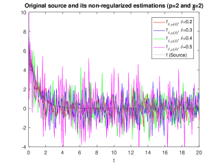
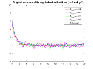
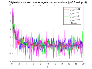
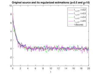
Figura 1: Example 1: Original Source and its estimations for the solution $f_{\delta}$ (left) and the regularized one $f_{\delta,\mu}$ (right) for the same set of noise levels.

$\delta$	0,01	0,02	0,03	0,04	0,05	0,06	0,07	0,08	0,09	0,1
$\|f-f_{\delta}\|$	9,54	9,59	9,62	9,75	10,09	10,17	10,283	10,90	11,85	12,19
$\|f-f_{\delta,\mu}\|$	5,282	5,305	5,307	5,309	5,310	5,315	5,318	5,320	5,326	5,369
Theoretical Bound	6,47	6,75	6,98	7,13	7,46	7,84	8,11	8,30	9,41	10,46

Cuadro 1: Example 1: Absolute non-regularized and regularized estimation errors and theoretical bound for example 5.1 assuming $p=2$ and data measured at $x_{0}=2$.

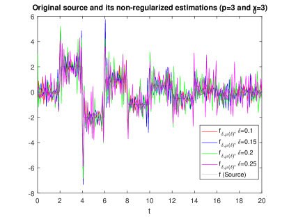
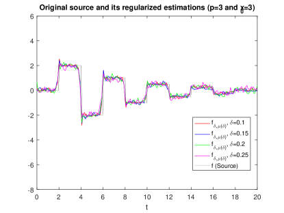
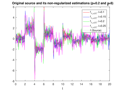
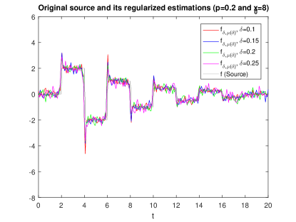
Figura 2: Example 2: Original Source and its estimations $f_{\delta}$ (left) and the regularized solution $f_{\delta,\mu}$ (right) for the same set of noise levels.

$\delta$	0,01	0,02	0,03	0,04	0,05	0,06	0,07	0,08	0,09	0,1
$\|f-f_{\delta}\|$	13,64	13,72	13,82	13,88	13,97	14,01	14,23	14,61	14,72	15,43
$\|f-f_{\delta,\mu}\|$	2,21	2,85	3,23	3,97	4,31	4,78	4,92	5,03	5,49	5,88
Theoretical Bound	2,37	3,13	3,68	4,13	4,52	4,86	5,17	5,46	5,72	5,97

Cuadro 2: Example 2: Absolute non-regularized and regularized estimation errors and theoretical bound for example 5.2 assuming $p=3$ and data measured at $x_{0}=3$.

6 Conclusions

We consider the inverse source problem for a 1D transport equation. We define a regularization family of operators to deal with the ill-posedness of the problem by compensation the instability factor in the inverse operator. We proposed a regularization parameter choice rule based on assumption of the noise level in data and the smoothness of the source to be identify. We prove that for the parameter choice rule proposed here, the method is stable and a Hölder type bound for the regularization error is obtained. The numerical examples show an improvement in the regularized solution with the respect to the one obtained when no regularization is applied. Numerical examples show good estimates for the source at different noise levels, in this work we have included few cases where the sources belong to different Hilbert spaces to illustrate the performance of this method.