Probabilistic Contrastive Learning for Domain Adaptation

Abstract

Contrastive learning can largely enhance the feature discriminability in a self-supervised manner and has achieved remarkable success for various visual tasks. However, it is undesirably observed that the standard contrastive paradigm (features+$\ell_{2}$ normalization) only brings little help for domain adaptation. In this work, we delve into this phenomenon and find that the main reason is due to the class weights (weights of the final fully connected layer) which are vital for the recognition yet ignored in the optimization. To tackle this issue, we propose a simple yet powerful Probabilistic Contrastive Learning (PCL), which does not only assist in extracting discriminative features but also enforces them to be clustered around the class weights. Specifically, we break the standard contrastive paradigm by removing $\ell_{2}$ normalization and replacing the features with probabilities. In this way, PCL can enforce the probability to approximate the one-hot form, thereby reducing the deviation between the features and class weights. Benefiting from the conciseness, PCL can be well generalized to different settings. In this work, we conduct extensive experiments on five tasks and observe consistent performance gains, i.e., Unsupervised Domain Adaptation (UDA), Semi-Supervised Domain Adaptation (SSDA), Semi-Supervised Learning (SSL), UDA Detection, and UDA Semantic Segmentation. Notably, for UDA Semantic Segmentation on SYNTHIA, PCL surpasses the sophisticated CPSL-D by $>\!2\%$ in terms of mean IoU with a much smaller training cost (PCL: 1*3090, 5 days v.s. CPSL-D: 4*V100, 11 days). Code is available at https://github.com/ljjcoder/Probabilistic-Contrastive-Learning.

1 Introduction

Deep neural networks with fully-supervised learning have made great progress in computer vision [36, 25, 27]. However, it requires the training data and test data to be collected from the same distribution, which always cannot be satisfied in real world. Unfortunately, applying the model trained on an old domain (source) to a new domain (target) often encounters a drastic performance degradation. To address the issue, domain adaptation [31, 50] has been proposed and attracted increasing attention.

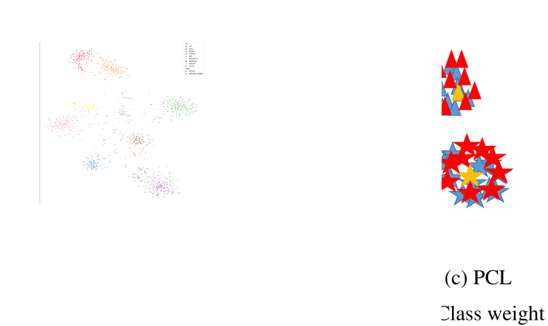
Figure 1: Feature Contrastive Learning (FSL) vs. Probabilistic Contrastive Learning (PCL). With PCL, the features on target domain can be clustered around the corresponding class weights.

For many visual tasks, the feature discriminability is the basis to obtain satisfying performance. However, in domain adaptation, the learned features for each class on target domain are usually diffuse as illustrated in Figure 1(a) since target domain lacks the ground-truth labels. This diffusion of features can lead to poor performance on the target domain, as the model struggles to accurately distinguish these features. Fortunately, contrastive learning is proposed to learn semantically similar features in a self-supervised manner [8, 81, 9, 32]. Inspired by its great success for representation learning, we perform the standard contrastive learning (features+$\ell_{2}$ normalization) to assist feature extraction on unlabeled target domain. However, we find that it only brings very limited improvement for domain adaptation (e.g., $64.3\%\rightarrow 64.5\%$ as shown in Figure 2). A natural question arises and motivates this work: Why does contrastive learning perform poorly in domain adaptation? In what follows, we will try to analyze the possible reason and provide the corresponding solution.

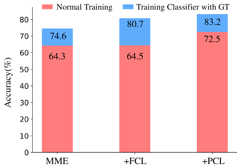
Figure 2: An explorative study under the Semi-Supervised Domain Adaptation (SSDA) setting on DomainNet (R$\rightarrow$S) [52] with 3-shot and ResNet34. We use MME [59] as a baseline model to verify the effect of FCL and PCL.

In most cases, the application scenario of domain adaptation focuses on the recognition field, e.g., image classification [16, 59], object detection [72, 18], semantic segmentation [92, 45]. For these tasks, the features are required to be not only discriminative themselves but also close to the class weights (i.e., the weights of the last fully connected layer). Nevertheless, the conventional contrastive learning mostly uses the features before the classifier to calculate the loss for supervision (dubbed as Feature Contrastive Learning or FCL for short), in which the vital class weights are not involved during optimization. Although the feature discriminability on target domain can be largely improved with FCL, due to the problem of domain shift, the features are still likely to be deviated from the corresponding class weights learned from source data as illustrated in Figure 1(b). To verify this assumption, we conduct an explorative study to freeze the feature extractor and train the classifier borrowing the ground-truth labels on target domain (not available in the normal training). As shown in Figure 2, the accuracy of FCL has increased by $6.1\%$ ($74.6\%\!\rightarrow\!80.7\%$) for such a setting, but the actual accuracy has only increased by 0.2$\%$ ($64.3\%\!\rightarrow\!64.5\%$). Based on these qualitative and quantitative analyses, we propose that the deviation between the features and class weights is the main reason leading to the poor performance of feature-based contrastive learning on domain adaptation.

To deal with the deviation, a naïve idea is to use the logits (i.e., the class scores output by the last fully connected layer) instead of the features to calculate the contrastive loss for supervision. However, we experimentally find that this approach cannot improve the performance of contrastive learning for domain adaptation. In this work, we try to solve this problem by carefully designing a new type of contrastive loss that can explicitly reduce the deviation between the features and class weights.

First, we try to dig out what kind of signal can effectively indicate that a feature vector is close to one of the class weights. For convenience, we define a set of class weights $W=(\mathbf{w}_{1},\mathbf{w}_{2},...,\mathbf{w}_{C})$, a feature vector $\mathbf{f}_{i}$, and its classification probability $\mathbf{p}_{i}$. Here $C$ is the number of classes and $p_{i,c}$ for the probability of $c$-th class is computed as

$$\small p_{i,c}=\frac{\exp(\mathbf{w}^{\top}_{c}\mathbf{f}_{i})}{\sum_{j\neq c}\exp(\mathbf{w}^{\top}_{j}\mathbf{f}_{i})+\exp(\mathbf{w}^{\top}_{c}\mathbf{f}_{i})}$$

Assuming $\mathbf{f}_{i}$ is close to $\mathbf{w}_{c}$, it means that $\mathbf{w}^{\top}_{c}\mathbf{f}_{i}$ is large and $p_{i,c}$ is close to 1. Meanwhile, $\{p_{i,j}\}_{j\neq c}$ will be close to $0$ since $\sum_{j}p_{i,j}=1$. In brief, when $\mathbf{f}_{i}$ is close to one of the class weights, the probability $\mathbf{p}_{i}$ will approximate the one-hot form.

Then, inspired by this intuition, we introduce a new member for the contrastive learning family, which is based on the probabilities and is thus dubbed as Probabilistic Contrastive Learning or PCL for short. Our approach can not only extract discriminative features on unlabeled target domain but also enforce them to be clustered around the class weights. Specifically, we break the standard contrastive paradigm by replacing the features with the probabilities and removing the $\ell_{2}$ normalization. Importantly, through these two simple operations, we successfully add a constraint on the probabilities on target domain to encourage them to approximate the one-hot form, which can largely reduce the deviation between the features and class weights. PCL is proposed as a concise yet powerful method to assist domain adaptation, which can be well generalized to different settings, including Unsupervised Domain Adaptation (UDA), Semi-Supervised Domain Adaptation (SSDA), Semi-Supervised Learning (SSL), UDA Detection, and UDA Semantic Segmentation. Simultaneously, it can be conveniently combined with various methods, e.g., GVB [16], MME [59], Fixmatch [64], CCSSL [86], Flexmatch [85], RPA [95], and BAPA [45]. And it is surprising that PCL outperforms many sophisticated counterparts, e.g., meta-optimization in MetaAlign [78] and prototypical+triplet loss in ECACL-P [40].

To summarize, our main contributions lie in three folds.

1) To the best of our knowledge, this is the first work to clearly point out that the standard contrastive learning cannot work well for domain adaptation since it does not consider the deviation between the features and class weights. It prompts us and the follow-up researchers to find new routes with contrastive learning instead of directly applying the standard paradigm to domain adaptation.

2) We propose a new self-supervised paradigm called Probabilistic Contrastive Learning for domain adaptation, which is concise from the perspective of implementation yet powerful for the generalization to different settings and various methods. As a new variant of contrastive learning, we believe PCL can also provide some useful insights for many other visual tasks [26, 49, 39].

3) Extensive experiments demonstrate that PCL can bring consistent performance improvement with different settings and various methods for domain adaptation. Particularly, PCL achieves state-of-the-art performance for UDA Semantic Segmentation and improve the mean IoU on SYNTHIA by $>\!2\%$ compared to the sophisticated CPSL-D [41] with a much smaller training cost (PCL: 1*3090, 5 days v.s. CPSL-D: 4*V100, 11 days).

2 Related Work

2.1 Contrastive Representation Learning

The core of contrastive learning is to bring the positive samples closer together and the negative samples farther away. Extensive works [8, 24, 23, 4, 12, 19] have shown that contrastive learning techniques can effectively learn more compact and transferable features. For example, SimCLR [8] uses self-supervised contrastive learning to first achieve the performance of a supervised ResNet-50 with only a linear classifier trained on self-supervised representations on full ImageNet. MoCo [24] and MoCo V2 [10] use a memory bank to make the model achieve competitive results even with a smaller batch size. These methods usually ignore class information, and treat samples belonging to the same category as negative samples, thereby pulling each other away. The latter SFCL [32] uses label information to eliminate wrong negative samples, effectively improving the performance of contrastive learning. All the above works conduct contrastive learning in the feature space and use the $\ell_{2}$ normalization to process the features. They do not explicitly consider reducing the deviation between features and class weights.

It is worth pointing out that TCL [63] is very similar to PCL in terms of implementation, because it uses the probability of $\ell_{2}$ normalization in the code. In essence, however, the two are fundamentally different. First of all, TCL does not find the problem of ”feature deviation from class weight” in traditional FCL, and naturally did not improve contrastive learning along this line of thought. Secondly, TCL does not realize the superiority of probability (the word “probability” does not even appear). It just happens to treat probability as a special feature and naturally still preserves the $\ell_{2}$ normalization operation. In essence, it is still a standard FCL framework (features+$\ell_{2}$ normalization).

In this paper, we will explicitly answer why the traditional FCL framework is not suitable for domain adaptation tasks? Why are probabilities necessarily superior to features? Why do we need to discard the $\ell_{2}$ normalization?

2.2 Domain Adaptation

Domain adaptation mostly focuses on the recognition field (e.g., image classification, object detection, semantic segmentation) and aims to transfer the knowledge from a labeled source domain to an unlabeled target domain. The literature can be roughly categorized into two categories.

The first category is to use domain alignment and domain invariant feature learning. For example, [70, 46, 47, 84] measure the domain similarity in terms of Maximum Mean Discrepancy (MMD) [3], while [65, 66, 52] introduce the metrics based on second-order or higher-order statistics. In addition, there are some methods [21, 69, 43, 60, 16] to learn domain-invariant features through adversarial training.

The second category is to learn discriminative representation using the pseudo-label technique [38, 40, 92, 22, 41]. Particularly, in domain adaptive semantic segmentation, recent high-performing methods [92, 41] commonly use the distillation techniques. Although distillation can greatly improve the accuracy, it interrupts the end-to-end training process, making model training very time-consuming. In addition, the distillation-based methods still use some special initialization tricks, such as ASOS [68] model for initialization in the first stage and SimCLRV2 [9] model for initialization in the distillation stage.

In this paper, we try to fully exploit the potential of contrastive learning for domain adaptation. Our method can be well generalized to classification, detection, and segmentation tasks. Particularly, in the domain adaptive semantic segmentation, PCL based on the non-distilled BAPA [45] can surpass CPSL-D [41] which uses complex distillation techniques as well as special initialization strategies.

2.3 Semi-Supervised Learning

Semi-supervised learning (SSL) [2, 37, 17, 87] aims to leverage the vast amount of unlabeled data with limited labeled data to improve the performance. Among the literature for SSL, pseudo-label-based methods have received more and more attention due to their simplicity and efficiency. For example, FixMatch [64] achieves impressive performance by generating the confident pseudo labels of the unlabeled samples and treating them as labels for the perturbed samples. Flexmatch [85] makes better use of unlabeled data by dynamically adjusting the threshold. Following this idea, Freematch [76] designed self-adaptive thresholding and self-adaptive class fairness regularization to adjust the threshold and beyond Flexmatch.

Although these methods have made great progress, SSL tasks still face the problem of unlabeled features deviating from class weights when the labeled data is scarce. Therefore, in this work, we also explore the effectiveness of PCL for SSL tasks.

3 Our approach

In this section, we first review feature contrastive learning (FCL) in the context of domain adaptation, and then elaborate on our probabilistic contrastive learning (PCL). We define the model $M=F\circ E$ with the feature extractor $E$ and the classifier $F$. Here $F$ has the parameters $W=(\mathbf{w}_{1},...,\mathbf{w}_{C})$, where $C$ is the number of classes and $\mathbf{w}_{k}$ is the class weights of the $k$-th class.

3.1 Feature Contrastive Learning

In the problem formulation for domain adaptation [70, 46, 47], the source domain images already have clear supervision signals, and the self-supervised contrastive learning is not urgently required. Thus we only calculate the contrastive loss (a.k.a., InfoNCE [51]) for the target domain data. Specifically, let $\mathcal{B}=\{\left(x_{i},\tilde{x}_{i}\right)\}_{i=1}^{N}$ be a batch of data pairs sampled from target domain, where $N$ is the batch size, and $x_{i}$ and $\tilde{x}_{i}$ are two random transformations of a sample. Then, we use $E$ to extract the features, and get $\mathcal{F}=\{(\mathbf{f}_{i},\tilde{\mathbf{f}}_{i})\}_{i=1}^{N}$. For a query feature $\mathbf{f}_{i}$, the feature $\tilde{\mathbf{f}}_{i}$ is the positive and all other samples are regarded as the negative. Then the InfoNCE loss has the following form:

$$\small\ell_{\mathbf{f}_{i}}=\!-\!\log\!\frac{\exp(sg(\mathbf{f}_{i}{})^{\top}g(\tilde{\mathbf{f}}_{i}))}{\sum\limits_{j\neq i}\!\exp(sg(\mathbf{f}_{i}{})^{\top}\!g(\mathbf{f}_{j}))+\sum\limits_{k}\!\exp(sg(\mathbf{f}_{i}{})^{\top}\!g(\tilde{\mathbf{f}}_{k}))},$$ (1)

where $g(\mathbf{f})=\frac{\mathbf{f}}{||\mathbf{f}||_{2}}$ is a standard $\ell_{2}$ normalization operation widely used in feature contrastive learning [51, 75, 8], and $s$ is the scaling factor.

From Eq (1), we can observe that there is no class weight information involved in $\ell_{\mathbf{f}_{i}}$. As a result, in the optimization process of contrastive loss, it is hardly possible to constrain the features to locate around the class weights.

3.2 A Naïve Solution

In order to involve the class weights during the optimization, a naïve solution is to use the logits (i.e., the class scores output by the classifier) for supervision. Therefore, we choose logits to calculate the contrastive loss as in Eq (1), and refer to it as Logits Contrastive Learning (LCL for short). However, this approach does not explicitly cluster the features to be close to the class weights and thus does not work experimentally. Therefore, we need to design a new type of contrastive loss to explicitly reduce the deviation between the features and class weights. More discussion about LCL will be provided in Section 4.2.

3.3 Probabilistic Contrastive Learning

The generalization ability of InfoNCE [51] has been fully verified in previous literature. In this work, instead of designing a totally different type of supervision, we focus on constructing a new input $\mathbf{f}^{\prime}_{i}$ to calculate the contrastive loss for the sake of making the feature $\mathbf{f}_{i}$ close to class weights. Formally, the loss about the new input $\mathbf{f}^{\prime}_{i}$ can be written in the following form:

$$\ell_{\mathbf{f}^{\prime}_{i}}=-\log\frac{\exp(s{\mathbf{f}^{\prime}_{i}}^{\top}\tilde{\mathbf{f}^{\prime}}_{i})}{\sum_{j\neq i}\exp(s{\mathbf{f}^{\prime}_{i}}^{\top}\mathbf{f}^{\prime}_{j})+\sum_{k}\exp(s{\mathbf{f}^{\prime}_{i}}^{\top}\tilde{\mathbf{f}^{\prime}}_{k})}.$$ (2)

Then our goal is to design a suitable $\mathbf{f}^{\prime}_{i}$ so that the smaller $\ell_{\mathbf{f}^{\prime}_{i}}$ is, the closer $\mathbf{f}_{i}$ is to the class weights.

From Eq (2), a smaller $\ell_{\mathbf{f}^{\prime}_{i}}$ means a larger ${\mathbf{f}^{\prime}_{i}}^{\top}\tilde{\mathbf{f}^{\prime}}_{i}$. Thus the above problem can be roughly simplified to the larger ${\mathbf{f}^{\prime}_{i}}^{\top}\tilde{\mathbf{f}^{\prime}}_{i}$ is, the closer $\mathbf{f}_{i}$ is to the class weights. On the other hand, as elaborated in Section 1, if $\mathbf{f}_{i}$ is close to the class weight, the corresponding probability ${\mathbf{p}_{i}}$ is approximate to the one-hot form:

$${\mathbf{p}_{i}}=(0,..,1,..,0).$$ (3)

Therefore, our goal can be reformulated as how to design a suitable $\mathbf{f}^{\prime}_{i}$ so that the larger ${\mathbf{f}^{\prime}_{i}}^{\top}\tilde{\mathbf{f}^{\prime}}_{i}$ is, the closer $\mathbf{p}_{i}$ is to the one-hot form.

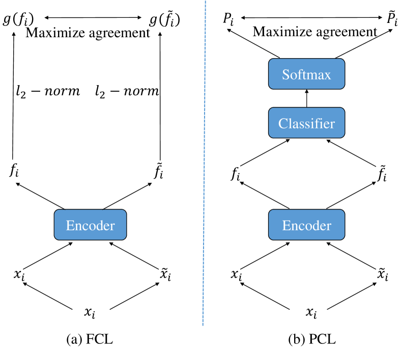
Figure 3: Framework of FCL and PCL. Different from FCL, PCL uses the output of softmax to perform contrastive learning and removes the $\ell_{2}$ normalization.

Fortunately, we found the probability $\mathbf{p}_{i}$ itself can meet such a requirement. Here we explain the mathematical details. Note that $\mathbf{p}_{i}=(p_{i,1},...,p_{i,C})$ and $\tilde{\mathbf{p}}_{i}=(\tilde{p}_{i,1},...,\tilde{p}_{i,C})$ are both the probability distributions. Then we have

$${0\leq p_{i,c}\leq 1},{0\leq\tilde{p}_{i,c}\leq 1},{\forall}c\in\{1,...,C\}.$$ (4)

In addition, the $\ell_{1}$-norm of $\mathbf{p}_{i}$ and $\tilde{\mathbf{p}}_{i}$ equals one, i.e., $||\mathbf{p}_{i}||_{1}=\sum_{c}p_{i,c}=1$ and $||\tilde{\mathbf{p}}_{i}||_{1}=\sum_{c}\tilde{p}_{i,c}=1$. Obviously, we have

$$\mathbf{p}_{i}{}^{\top}\tilde{\mathbf{p}}_{i}=\sum_{c}p_{i,c}\tilde{p}_{i,c}\leq 1.$$ (5)

The equality is held if and only if $\mathbf{p}_{i}=\tilde{\mathbf{p}}_{i}$ and both of them have a one-hot form as in Eq (3). In other words, in order to maximize $\mathbf{p}_{i}^{\top}\tilde{\mathbf{p}}_{i}$, the $\mathbf{p}_{i}$ and $\tilde{\mathbf{p}}_{i}$ need satisfy the one-hot form at the same time. Therefore, $\mathbf{p}_{i}$ can server as the new input $\mathbf{f}^{\prime}_{i}$ in Eq (2).

Importantly, from the above derivation process, we can see that the property that the $\ell_{1}$-norm of probability equals one is very important. This property guarantees that the maximum value of $\mathbf{p}_{i}^{\top}\tilde{\mathbf{p}}_{i}$ can only be reached when $\mathbf{p}_{i}$ and $\tilde{\mathbf{p}}_{i}$ satisfy the one-hot form at the same time. Evidently, we cannot perform $\ell_{2}$ normalization operation on probabilities like the traditional FCL. Finally, our new contrastive loss is defined by

$$\ell_{\mathbf{p}_{i}}=-\log\frac{\exp(s{\mathbf{p}_{i}}^{\top}\tilde{\mathbf{p}}_{i})}{\sum_{j\neq i}\exp(s{\mathbf{p}_{i}}^{\top}\mathbf{p}_{j})+\sum_{k}\exp(s{\mathbf{p}_{i}}^{\top}\tilde{\mathbf{p}}_{k})}.$$ (6)

Comparing Eq (1) and Eq (6), we can see two main differences. First, Eq (6) uses the probability $\mathbf{p}_{i}$ in contrastive learning instead of the extracted features $\mathbf{f}_{i}$. Second, Eq (6) removes the $\ell_{2}$ normalization $g$. Figure 3 gives an intuitive comparison between FCL and PCL. It is worth emphasizing that, the rationale behind PCL is the core value of this work, which leads to a convenient implementation. Benefiting from the conciseness, PCL can well generalized to different settings and various methods.

4 Discussion and Comparison

In the section, we try to verify the necessity and rationality of PCL through both qualitative and quantitative analyses. In particular, we will focus on answering the following three questions:

1. One of the core contributions of this paper is the discovery that ”reducing the deviation between features and class weights is the key to the problem of whether contrastive learning can be successfully applied in DA tasks”. If it is not based on this motivation, can we achieve the performance of PCL or directly induce PCL through some technologies similar to PCL, such as the projection head, consistency of prediction space?

2. Could simply approximating the probabilities to the one-hot form substantially improve the performance of FCL without having to keep the InfoNCE form?

3. Many works [19, 32, 81] have shown that alleviating the false negative problem can effectively improve the performance of contrastive learning. Therefore, can we also solve the false negative problem to effectively improve the poor performance of FCL in domain adaptation tasks without using PCL?

4. Does PCL really effectively reduce the deviation between features and class weights?

For the quantitative analysis, the typical semi-supervised domain adaptation (SSDA) setting on DomainNet [52] with 3-shot and ResNet34 is adopted as the benchmark. We believe these analyses can also provide some useful insights for other visual tasks [26, 49, 39].

4.1 PCL v.s. FCL

Current approaches based on FCL [62, 63, 99] generally regard contrastive learning as a general technique to improve feature consistency and often focus on the false negative sample problem. Few works consider the shortcomings of contrastive learning in domain adaptation tasks from the perspective of the deviation of features and class weights. Therefore, we believe that analyzing and finding this shortcoming is not a trivial result. Based on the above insights, we deduce a concise PCL through in-depth analysis. We surprisingly found that only two simple operations (using probabilities and removing $\ell_{2}$ normalization) are needed to force features close to class weights.

Experimentally, we compare contrastive learning based on features (FCL) and probabilities (PCL), and present the results in Table 1. First, the traditional FCL can improve the performance of the baseline but the gain is limited. Second, the average gain of our probabilistic contrastive learning over FCL is more than 5$\%$, which indicates the valuable effect of probabilistic contrastive learning.

Method	R$\rightarrow$C	R$\rightarrow$P	P$\rightarrow$C	C$\rightarrow$S	S$\rightarrow$P	R$\rightarrow$S	P$\rightarrow$R	Mean
Baseline	71.4	70.0	72.6	62.7	68.2	64.3	77.9	69.5
+ FCL	72.5	71.6	73.1	66.4	70.2	64.5	80.8	71.3
+ NTCL	72.9	71.3	73.3	66.3	71.3	67.1	80.5	71.7
+ LCL	72.8	70.6	72.5	66.4	70.5	64.5	81.3	71.2
+ Our PCL-$\ell_{2}$	75.1	74.4	76.2	70.3	73.5	69.9	82.5	74.6
+ Our PCL	78.1	76.5	78.6	72.5	75.6	72.5	84.6	76.9

Table 1: Ablation study on effect of different features on DomainNet under the setting of $3$-shot and Resnet34.

4.2 PCL v.s. FCL with Projection Head

In SimCLR [8], the authors have proven that projection head is a very useful technique. It changes the feature of calculating the contrastive loss from feature+$\ell_{2}$ normalization to projection head+$\ell_{2}$ normalization. Inspired by this, CLDA [62] uses the classifier as the projection head to design two contrastive learning losses and achieve better performance. In this section, we mainly verify whether the performance gain of our PCL comes from the application of projection head. To this end, we designed the following three types of projection heads:

(1) Following the SimCLR, we introduce an additional nonlinear transformation (NT) on the features, and then normalize the features after the NT to calculate the contrastive loss. We call it NT-Based Contrastive Learning (NTCL).

(2) We directly use the classifier as the projection head and named it Logits Contrastive Learning (LCL for short). Since LCL uses the output after the classifier to calculate the contrastive loss, it is one of the most direct methods to introduce class weight information.

(3) We further generalize the projection head to classifier+softmax. For this setting, the feature of calculating the contrastive loss becomes classifier+softmax with $\ell_{2}$ normalization. Essentially, it has only one more $\ell_{2}$ normalization than our PCL, and thus we denote it PCL-$\ell_{2}$. Like LCL, PCL-$\ell_{2}$ is also a way to introduce class weight information. However, it is worth noting that PCL-$\ell_{2}$ is not a natural extension of the projection head technique, since many current contrastive learning methods  [8, 19, 12, 11] do not include softmax in the projection head. In this section, the projection head is extended to the form of classifier + softmax in order to verify such a question: when probability is used as a special feature, can the traditional contrastive learning paradigm (feature + $\ell_{2}$ normalization) be as effective as PCL?

Table 1 gives the experimental results and we obtain the following observations. First, the above three projection heads all get lower performance than PCL, which indicates that the key reason for the gain of PCL is not from the use of the projection head. Second, both LCL and PCL-$\ell_{2}$ are inferior to PCL, which shows that simply introducing class weight information cannot effectively enforce features to locate around class weights. Thus, it is necessary to deliberately design a contrastive learning loss to explicitly constrain the distance of feature and class weights. Third, the results experimentally verify the motivation of PCL. The current contrastive learning methods [19, 12, 11] all follow the standard paradigm of feature+$\ell_{2}$ normalization. In particular, neither the perspective of the projection head nor the introduction of class weights can lead to PCL since there is no reason for them to adopt probability nor is there a reason to discard the $\ell_{2}$ normalization widely used in contrastive learning. In this work, however, our motivation is exactly that contrastive learning needs to reduce the deviation between the features and class weights for domain adaptation. Therefore, we can confidently point out that the features need to be replaced by probabilities and the $\ell_{2}$ normalization should be removed (in section 3.3).

4.3 Cosine distance v.s. MSE distance

In domain adaptation, there has been a work [20] that exploits the similarity of the prediction space for consistency constraints, although it does not use the form of contrastive learning. Intuitively, PCL seems to just apply this idea to the contrastive learning loss (transfer feature space to prediction space). Then we need to answer an important question: Is PCL effective only because of the consistency constraint in the prediction space?

From the previous analysis, it can be seen that the goal of PCL is to make the features close to the class weights by enforcing the probabilities to appear in the one-hot form, rather than to achieve the consistency constraint of the output space. It is just that we found that contrastive learning in the form of probability inner product (cosine distance) can achieve the goal. To verify it, we replace the inner product in PCL with the MSE used in  [20] to get PCL-MSE. Table 2 gives the results. It can be seen that PCL is better than PCL-MSE. This is because mse can only make the probability similar but not make the probability appear the one-hot form. This again proves the importance of the motivation of PCL, because this motivation ensures that PCL must use the cosine distance but not the MSE distance.

4.4 The Importance of InfoNCE Loss

Method	R$\rightarrow$C	R$\rightarrow$P	P$\rightarrow$C	C$\rightarrow$S	S$\rightarrow$P	R$\rightarrow$S	P$\rightarrow$R	Mean
Baseline	71.4	70.0	72.6	62.7	68.2	64.3	77.9	69.5
+ FCL	72.5	71.6	73.1	66.4	70.2	64.5	80.8	71.3
+ SFCL	72.7	72.4	73.2	66.5	70.8	65.5	81.2	71.8
+ BCE	73.3	73.0	74.7	66.7	71.9	67.5	80.4	72.5
+ FCL+BCE	73.9	73.1	74.1	66.5	71.5	67.3	81.4	72.5
+ Our PCL-MSE	76.6	75.3	76.2	69.7	74.2	70.5	83.8	75.1
+ PCL	78.1	76.5	78.6	72.5	75.6	72.5	84.6	76.9

Table 2: Comparison of different FCL improvement methods on DomainNet under the setting of $3$-shot and Resnet34.

In this section, we explore whether it is necessary to use the function form based on InfoNCE loss to approximate the probability to the one-hot form. In particular, we consider binary cross entropy loss (BCE) used in [97]. For convenience, we redefine the probabilities $\mathbf{p}_{i}$ and $\tilde{\mathbf{p}_{i}}$ as $\mathbf{p}_{i}^{0}$ and $\mathbf{p}_{i}^{1}$. Then the new loss function is defined as

$$\ell_{bce}\!=\!-\!\!\!\sum_{i,j,m,n}\!(\hat{y}^{n,m}_{i,j}\!\log\left(p^{n,m}_{i,j}\right)\!+\!\left(1\!-\!\hat{y}^{n,m}_{i,j}\right)\log(1-p^{n,m}_{i,j})),$$ (7)

where $n,m\in\{0,1\}$, $p^{n,m}_{i,j}={\mathbf{p}^{n}_{i}}^{\top}\mathbf{p}^{m}_{j}$, and $\hat{y}^{n,m}_{i,j}=\mathbbm{1}[p^{n,m}_{i,j}\geq t$ or $(i=j)]$. We use $t=0.95$ for the quantitative analyses.

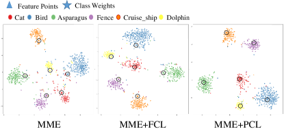
Figure 4: The t-SNE visualization of learned features. We focus on the relationship between features and class weights on the R$\rightarrow$S task of DomainNet dataset with Resnet34 under the setting of $3$-shot. Best viewed in color.

Observing Eq (7), BCE loss will maximize $p^{n,m}_{i,j}={\mathbf{p}^{n}_{i}}^{\top}\mathbf{p}^{m}_{j}$ when $\hat{y}^{n,m}_{i,j}=1$. Note that $\mathbf{p}^{n}_{i}$ and $\mathbf{p}^{m}_{j}$ are the probability. So $p^{n,m}_{i,j}$ will take maximum if and only if $\mathbf{p}^{n}_{i}$ and $\mathbf{p}^{m}_{j}$ are equal and both of them have a one-hot form. Therefore, BCE loss can force the probability to present the one-hot form. Based on the above analysis, we can use BCE to replace PCL. In addition, we also consider combining FCL and BCE to optimize the model. Table 2 gives the results. It can be seen that although the BCE is better than FCL, it is still inferior to PCL. This indicates that the form of InfoNCE is better than the pair-wise form of BCE, and the conclusion is consistent with [73].

4.5 PCL v.s. SFCL

In contrastive learning, there may be some negative samples that indeed belong to the same category as the query sample, which are called false negative samples. Many methods [19, 32, 81] point out that false negative samples are harmful to contrastive learning. In this section, we try to answer another important question: whether can we make feature contrastive learning work well by reducing the false negative samples without probabilistic contrastive learning?

An appropriate way to address the false negative problem is to use supervised feature contrastive learning (SFCL) [32]. Since the target domain data has no labels, we regard samples with a similarity greater than 0.95 to the query sample as false negative samples and remove them from the denominator.

Table 2 shows the experimental comparison. It can be seen that SFCL can indeed improve the performance of FCL. However, compared with PCL, SFCL has a very limited improvement over FCL. Specifically, SFCL can learn better feature representations by alleviating the false negative problem, but it cannot solve the problem of the deviation between the features and class weights. The experimental results reveal that the deviation problem is more critical than the negative samples for domain adaptation.

4.6 Visualization Analysis

Figure 4 shows the relationship between the unlabeled features and the class weights for the three methods, including MME, MME+FCL, and MME+PCL. Firstly, compared with MME, MME+FCL produces more compact feature clusters for the same category and more separate feature distributions for different categories. However, the learned class weights are deviated from the feature centers for both MME+FCL and MME. Secondly, the class weights of MME+PCL are much closer to the feature centers than MME+FCL. It demonstrates that PCL is significantly effective in enforcing the features close to the class weights.

5 Experiments

In this section, we will verify the validity of the PCL on five different tasks. Four of these are classification, detection, and segmentation tasks in domain adaptation, and one is a semi-supervised learning task under conditions with little labeled data. For more experimental details and results, please refer to Section  7 and Section  8.

5.1 UDA Semantic Segmentation

Methods	GTA5	SYNTHIA
	mIoU (%)	mIoU-13 (%)	mIoU-16 (%)
ProDA ( CVPR’21 ) [92]	53.7	-	-
DSP ( ACM MM’21 ) [22]	55.0	59.9	51.0
CPSL( CVPR’22 ) [41]	55.7	61.7	54.4
BAPA ( ICCV’21 ) [45]	57.4	61.2	53.3
ProDA-D ( CVPR’21 ) [92]	57.5	62.0	55.5
MFA-D (BMVC’21) [91]	58.2	62.5	-
ProDA-D+CaCo ( CVPR’22 ) [28]	58.0	-	-
CPSL-D ( CVPR’22 ) [41]	60.8	65.3	57.9
BAPA∗	57.7	60.1	53.3
+ Our PCL	60.7	68.2	60.3

Table 3: Result on UDA Semantic Segmentation. -D means to use an additional two-step distillation technique. ${*}$ means our reimplementation. For more detailed experimental results, please refer to the supplementary material.

Setup We evaluate the performance of our methods on two standard UDA semantic segmentation tasks: GTA5 [57]$\rightarrow$Cityscapes [14] and SYNTHIA [58]$\rightarrow$Cityscapes. We take BAPA [45] with ResNet-101 [25] as our baseline.

The current SOTA method of UDA semantic segmentation generally adopts the distillation technique for post-processing. The distillation makes the training process very complicated and requires some special training strategies, such as initialization with a more transferable SimCLRV2 [9] model. Therefore, here we divide UDA semantic segmentation methods into simple non-distilled methods and complex distillation methods.

Table 3 gives the results. First, our method can achieve very significant gains on the baseline and outperforms all non-distilled methods by a large margin on SYNTHIA (6.5$\%$ for mIoU-13 and 5.9$\%$ of mIoU-16). Second, compared with the methods using distillation techniques, our method has only slightly lower performance than CPSL-D on GTA5 and outperforms CPSL-D by more than 2$\%$ on SYNTHIA. Notably, the training cost of the distillation-based methods is particularly expensive. For example, CPSL-D requires 4*V100 and a training period of 11 days, while our method only needs 1*RTX3090 and a training period of about 5 days.

5.2 UDA Classification

Setup We evaluate our PCL in the following two standard benchmarks: Office-Home [71] and VisDA-2017 [53]. We take GVB-GD [16] with ResNet50 [25] as our baseline.

Method	Acc	Method	Acc
RADA ( ICCV’21 ) [29]	71.4	ToAlign ( NeurIPS’21 )  [79]	72.0
SCDA ( ICCV’21 ) [42]	73.1	FixBi ( CVPR’21 ) [50]	72.7
SDAT ( ICML’22 ) [55]	72.2	BNM (CVPR’20) [15]	69.4
NWD ( CVPR’22 ) [6]	72.6	CTS ( NeurIPS’21 ) [44]	73.0
GVB* ( CVPR’20 ) [16]	70.3	GVB†	73.5
+ MetaAlign ( CVPR’21 ) [78]	71.3	-	-
+ Our PCL	72.3	+ Our PCL	74.5

Table 4: Average performance of 12 UDA tasks on Office-Home. * means our reimplementation. For more detailed experimental results, please refer to the supplementary material.

Method	Acc	Method	Acc
CST ( NeurIPS’21 ) [44]	80.6	SENTRY ( ICCV’21 ) [54]	76.7
GVB* ( CVPR’21 ) [16]	75.0	GVB†	80.4
+ Our PCL	80.8	+ Our PCL	82.5

Table 5: Accuracies(%) of Synthetic$\rightarrow$Real on VisDA-2017 for UDAs. * means our reimplementation.

Table 4 and Table 5 give the results. In particular, inspired by some previous semi-supervised domain adaptation methods [38, 40], we add FixMatch [64] to GVB and get the stronger GVB^†. We evaluate our proposed method by applying PCL to GVB and GVB^†. From the results, it can be seen that our method can bring considerable gains both on GVB and GVB^†. In particular, with GVB as the baseline, PCL outperforms MetaAlign by $1\%$, which is a meta-optimization-based technique and involves more complicated operations than PCL. This further demonstrates the superiority of PCL.

5.3 Semi-Supervised Domain Adaptation

Methods	Office-Home	DomainNet
	3-shot	1-shot	3-shot
CLDA ( NeurIPS’21 )  [62]	75.5	71.9	75.3
MME∗ ( ICCV’19 ) [59]	73.5	67.9	69.5
+ Our PCL	75.5	73.5	76.9
CDAC† ( CVPR’21 ) [38]	74.8	73.6	76.0
ECACL-P† ( ICCV’21 ) [40]	-	72.8	76.4
MCL† ( IJCAI’22 ) [85]	77.1	74.4	76.5
MME†	76.9	72.9	76.1
+ Our PCL	78.1	75.1	78.2

Table 6: Average performance on DomainNet (7 SSDA tasks) and Office-Home (12 SSDA tasks). ${*}$ means our reimplementation. For more detailed experimental results, please refer to the supplementary material.

Setup We evaluate the effectiveness of our proposed approach on two SSDA image classification benchmarks, i.e., DomainNet [52] and Office-Home. We choose MME [59] with ResNet34 [25] as our baseline. In particular, inspired by CDAC [38] and ECACL-P [40], we add FixMatch [64] to MME to build a stronger MME^†.

Table 6 gives the results and we have the following observations.

1) PCL outperforms the methods without Fixmatch for most of settings. In particular, CLDA uses a classifier as the projection head with instance contrastive learning and class-wise contrastive learning. But our PCL can defeat CLDA, although PCL is only equipped with instance contrastive learning. For example, under the DomainNet, PCL achieves 73.5$\%$ (1-shot) and 76.9$\%$ (3-shot) while CLDA achieves 71.9$\%$ (1-shot) and 75.3$\%$ (3-shot). The results indicate the superiority of PCL over the projection head.

2) Both CDAC and ECACL-P use Fixmatch. In addition, CDAC proposes the AAC loss to improve MME loss, while ECACL-P designs the prototypical loss and triplet loss to further improve MME performance. It can be seen that PCL is close to CDAC and ECACL-P in performance even without Fixmatch, and once equipped with Fixmatch, our method achieves state-of-the-art for almost all settings. It proves that PCL outperforms the AAC loss and prototypical loss+triplet loss.

5.4 UDA Detection

Setup We conduct an experiment on SIM10k [30] $\rightarrow$ Cityscapes [14] scenes to verify whether our proposed method is effective for the object detection task. In particular, we choose the RPA [95] with Vgg16 [61] as the baseline. In the experiment, we add PCL to the classification head to improve the classification results of the RPA model.

Table 7 gives the results. It can be seen that our method can still improve the performance of the baseline model on UDA detection.

Method	AP	Method	AP
MeGA-CDA ( CVPR’21 ) [72]	44.8	RPA ( CVPR’21 )∗ [95]	45.3
UMT ( CVPR’21 ) [18]	43.1	+ Our PCL	47.8

Table 7: Detection performance (%) on UDA detection task. ${*}$ means our reimplementation.

5.5 Semi-Supervised Learning

Method	4-shot Acc	Method	4-shot Acc
Dash ( ICML’21 ) [83]	55.24$\pm$0.96	SimMatch ( CVPR’22 ) [96]	62.19
DP-SSL ( NeurIPS’21 ) [82]	56.83$\pm$1.29	NP-Match ( ICML’21 ) [74]	61.09$\pm$0.99
Freematch ( ICLR’23 ) [76]	62.02$\pm$0.42	Softmatch ( ICLR’23 ) [5]	62.90$\pm$0.77
FixMatch* ( NeurIPS’20 ) [64]	53.58$\pm$ 2.09	+ Our PCL	57.62$\pm$2.52
CCSSL* ( CVPR’22 ) [86]	60.49$\pm$0.57	+ Our PCL	62.95$\pm$1.39
FlexMatch* ( NeurIPS’21 ) [90]	61.78$\pm$ 1.17	+ Our PCL	64.15$\pm$0.53

Table 8: Accuracy of SSL for CIFAR-100 (400 labels). * means our reimplementation.

In fact, the applicable scenarios of PCL are not limited to the domain adaptation. As long as the features of unlabeled data cannot be clustered around the class weights, our method has good potential to improve the performance. In this section, we consider the case where the source domain and target domain come from the same distribution, i.e., semi-supervised learning. In particular, for the semi-supervised tasks, the unlabeled features will deviate from the class weight when the labeled data is very scarce. Therefore, we consider the case where there are only 4 labeled samples per class.

Setup We conduct the experiments on CIFAR-100 [35].We take FixMatch [64], CCSSL [86] and Flexmatch [90] as our baseline and use WRN-28-8 [89] as backbone.

The quantitative evaluation results on CIFAR-100 are reported in Table 8. Our method gets a great gain (+4.04$\%$) for FixMatch. On the stronger baseline model CCSSL and Flexmatch, our PCL still get a significant gain. The results well demonstrate the effectiveness of our method.

6 Conclusion

In this paper, we found that the traditional FCL can only cluster the features of similar semantics and cannot enforce the learned features to be distributed around the class weights because the class weights are not involved during optimization. To solve this problem, we propose a novel probabilistic contrastive learning. Specifically, we use the probabilities after Softmax instead of the features, and remove the $\ell_{2}$ normalization widely used in FCL. We experimentally verified the effectiveness of our proposed methods in multiple tasks and multiple methods. We believe that our PCL provides an innovative route for various visual tasks.

	Method	road	sdwk	bld	wall	fnc	pole	lght	sign	veg.	trrn.	sky	pers	rdr	car	trck	bus	trn	mtr	bike	mIoU
	DACS (WACV’20) [67]	89.9	39.7	87.9	30.7	39.5	38.5	46.4	52.8	88.0	44.0	88.8	67.2	35.8	84.5	45.7	50.19	0.0	27.3	34.0	52.1
	SPCL (arXiv’21)  [80]	90.3	50.3	85.7	45.3	28.4	36.8	42.2	22.3	85.1	43.6	87.2	62.8	39.0	87.8	41.3	53.9	17.7	35.9	33.8	52.1
	RCCR (arXiv’21) [98]	93.7	60.4	86.5	41.1	32.0	37.3	38.7	38.6	87.2	43.0	85.5	65.4	35.1	88.3	41.8	51.6	0.0	38.0	52.1	53.5
	SAC (arXiv’21) [1]	90.4	53.9	86.6	42.4	27.3	45.1	48.5	42.7	87.4	40.1	86.1	67.5	29.7	88.5	49.1	54.6	9.8	26.6	45.3	53.8
	Pixmatch (CVPR’21) [48]	91.6	51.2	84.7	37.3	29.1	24.6	31.3	37.2	86.5	44.3	85.3	62.8	22.6	87.6	38.9	52.3	0.7	37.2	50.0	50.3
	ProDA (CVPR’2021) [92]	-	-	-	-	-	-	-	-	-	-	-	-	-	-	-	-	-	-	-	53.7
	DPL (ICCV’21) [13]	92.8	54.4	86.2	41.6	32.7	36.4	49.0	34.0	85.8	41.3	83.0	63.2	34.2	87.2	39.3	44.5	18.7	42.6	43.1	53.3
	BAPA (ICCV’21) [45]	94.4	61.0	88.0	26.8	39.9	38.3	46.1	55.3	87.8	46.1	89.4	68.8	40.0	90.2	60.4	59.0	0.00	45.1	54.2	57.4
	UPST (ICCV’21) [77]	90.5	38.7	86.5	41.1	32.9	40.5	48.2	42.1	86.5	36.8	84.2	64.5	38.1	87.2	34.8	50.4	0.2	41.8	54.6	52.6
	DSP (ACM MM’21) [22]	92.4	48.0	87.4	33.4	35.1	36.4	41.6	46.0	87.7	43.2	89.8	66.6	32.1	89.9	57.0	56.1	0.0	44.1	57.8	55.0
	CPSL (CVPR’22) [41]	91.7	52.9	83.6	43.0	32.3	43.7	51.3	42.8	85.4	37.6	81.1	69.5	30.0	88.1	44.1	59.9	24.9	47.2	48.4	55.7
	MFA-D (BMVC’21) [91]	93.5	61.6	87.0	49.1	41.3	46.1	53.5	53.9	88.2	42.1	85.8	71.5	37.9	88.8	40.1	54.7	0.0	48.2	62.8	58.2
	ProDA-D (CVPR’21) [92]	87.8	56.0	79.7	46.3	44.8	45.6	53.5	53.5	88.6	45.2	82.1	70.7	39.2	88.8	45.5	59.4	1.0	48.9	56.4	57.5
	ProDA-D + CaCo (CVPR’22) [28]	93.8	64.1	85.7	43.7	42.2	46.1	50.1	54.0	88.7	47.0	86.5	68.1	2.9	88.0	43.4	60.1	31.5	46.1	60.9	58.0
	ProDA-D + CRA (arXiv’21) [75]	89.4	60.0	81.0	49.2	44.8	45.5	53.6	55.0	89.4	51.9	85.6	72.3	40.8	88.5	44.3	53.4	0.0	51.7	57.9	58.6
	CPSL-D (CVPR’2022) [41]	92.3	59.9	84.9	45.7	29.7	52.8	61.5	59.5	87.9	41.5	85.0	73.0	35.5	90.4	48.7	73.9	26.3	53.8	53.9	60.8
	BAPA*	94.1	61.5	87.6	38.4	37.9	37.4	46.7	59.2	88.0	47.0	88.3	69.0	32.1	91.2	62.8	61.7	0.6	42.9	49.9	57.7
	+ Our PCL	95.6	71.0	89.1	46.8	43.4	45.8	53.5	64.1	88.3	43.3	87.6	70.9	44.5	89.8	57.9	61.5	0.0	42.4	58.5	60.7

Table 9: Results on the GTA5$\rightarrow$Cityscapes benchmark. D means using distillation technique.

	Method	road	sdwk	bld	wall∗	fnc∗	pole∗	light	sign	veg.	sky	pers	rdr	car	bus	mtr	bike	mIoU-16	mIoU-13
	DACS (WACV’20) [67]	80.6	25.1	81.9	21.5	2.9	37.2	22.7	24.0	83.7	90.8	67.6	38.3	82.9	38.9	28.5	47.6	48.3	54.8
	SPCL (arXiv’21) [80]	86.9	43.2	81.6	16.2	0.2	31.4	12.7	12.1	83.1	78.8	63.2	23.7	86.9	56.1	33.8	45.7	47.2	54.4
	RCCR (arXiv’21) [98]	79.4	45.3	83.3	-	-	-	24.7	29.6	68.9	87.5	63.1	33.8	87.0	51.0	32.1	52.1	-	56.8
	SAC (CVPR’21) [1]	89.3	47.2	85.5	26.5	1.3	43.0	45.5	32.0	87.1	89.3	63.6	25.4	86.9	35.6	30.4	53.0	52.6	59.3
	Pixmatch (CVPR’21) [48]	92.5	54.6	79.8	4.8	0.1	24.1	22.8	17.8	79.4	76.5	60.8	24.7	85.7	33.5	26.4	54.4	46.1	54.5
	DPL (ICCV’21) [13]	87.5	45.7	82.8	13.3	0.6	33.2	22.0	20.1	83.1	86.0	56.6	21.9	83.1	40.3	29.8	45.7	47.0	54.2
	BAPA (ICCV’21) [45]	91.7	53.8	83.9	22.4	0.8	34.9	30.5	42.8	86.6	88.2	66.0	34.1	86.6	51.3	29.4	50.5	53.3	61.2
	UPST (ICCV’21) [77]	79.4	34.6	83.5	19.3	2.8	35.3	32.1	26.9	78.8	79.6	66.6	30.3	86.1	36.6	19.5	56.9	48.0	54.6
	DSP (ACM MM’21) [22]	86.4	42.0	82.0	2.1	1.8	34.0	31.6	33.2	87.2	88.5	64.1	31.9	83.8	65.4	28.8	54.0	51.0	59.9
	CPSL-D (CVPR’22) [41]	87.2	43.9	85.5	33.6	0.3	47.7	57.4	37.2	87.8	88.5	79.0	32.0	90.6	49.4	50.8	59.8	57.9	65.3
	MFA-D (BMVC’2021)  [91]	81.8	40.2	85.3	-	-	-	38.0	33.9	82.3	82.0	73.7	41.1	87.8	56.6	46.3	63.8	-	62.5
	ProDA-D (CVPR’2021) [92]	87.8	45.7	84.6	37.1	0.6	44.0	54.6	37.0	88.1	84.4	74.2	24.3	88.2	51.1	40.5	45.6	55.5	62.0
	ProDA-D + CRA (arXiv’2021) [75]	85.6	44.2	82.7	38.6	0.4	43.5	55.9	42.8	87.4	85.8	75.8	27.4	89.1	54.8	46.6	49.8	56.9	63.7
	CPSL-D (CVPR’2022)  [41]	87.2	43.9	85.5	33.6	0.3	47.7	57.4	37.2	87.8	88.5	79.0	32.0	90.6	49.4	50.8	59.8	57.9	65.3
	BAPA*	71.0	36.8	76.8	26.0	4.2	40.8	39.1	35.4	88.7	88.6	69.7	34.3	89.1	62.8	43.7	45.3	53.3	60.1
	+ Our PCL	91.2	63.1	84.7	30.3	6.7	42.2	47.4	49.6	89.4	91.3	70.2	39.2	91.4	66.8	44.7	57.1	60.3	68.2

Table 10: Results on the SYNTHIA$\rightarrow$Cityscapes benchmark. mIoU-16 and mIoU-13 refer to mean intersection-over-union on the standard sets of 16 and 13 classes, respectively. Classes not evaluated are replaced by ’*’. D means using distillation technique.

7 Implementation Details

7.1 UDA Semantic Segmentation

Following the widely used UDA Semantic segmentation protocols [67, 48, 98, 45], we use the DeepLab-v2 segmentation model [7] with a ResNet-101 [25] backbone pre-trained on ImageNet as our model. Following [48], we first perform warm-up training on source domain. We adopt SGD with momentum of 0.9 and set the weight decay to $5\times 10^{-4}$. The learning rate is set at $2.5\times 10^{-4}$ for backbone and $2.5\times 10^{-3}$ for others. During training we use a poly policy with an exponent of 0.9 for learning rate decay. The max iteration number is set to 250k. For the hyper-parameters in PCL, we set $s=20$ in all experiments.

7.2 UDA

Following the standard transductive setting [16] for UDA, we use all labeled source data and all unlabeled target data, and test on the same unlabeled target data. For model selection, we use ResNet-50 [25] pre-trained on ImageNet as the backbone network for both Office-Home and VisDA-2017. For training hyper-parameters, we use mini-batch stochastic gradient descent (SGD) with a momentum of 0.9 and a weight decay of 0.001. For Office-Home, the initial learning rate is set to 0.001. For VisDA-2017, an initial learning rate of 0.0003 is used. The max iteration number is set to 10k.

When applying FixMatch in domain adaptation task, there exist wrong predicted high confident target samples, which can hurt the performance in the target domain. To amend this, we follow [92, 40] which uses a regularization term from [100]. It encourages the high confident output to be evenly distributed to all classes. For the hyper-parameters in PCL, we set $s=7$ in all experiments.

$$\ell_{reg}=-\sum_{i=1}^{N}\sum_{j=1}^{C}\frac{1}{C}\log p_{t}^{(i,j)}.$$ (8)

where $N$ denotes for the number of high confident samples, $C$ denotes for the number of classes.

7.3 SSDA

Following MME [59], we remove the last linear layer of AlexNet and ResNet34, while adding a new classifier $F$. We also use the model pre-trained on ImageNet to initialize all layers except $F$. We adopt SGD with momentum of 0.9 and set the initial learning rate is 0.01 for fully-connected layers whereas it is set 0.001 for other layers. The max iteration number is set to 50k. In SSDA task, we also use the regularization term in Equation (8). For the hyper-parameters in PCL, we set $s=7$ in all experiments.

7.4 UDA Detection

Following [95], we adopt the Faster R-CNN [56] with VGG16 [61] as backbone and initialized by the model pre-trained on ImageNet. We follow the original papers [95] and train the model for 80k iterations. The training strategies of detector and discriminator are also consistent with RPN. For detector, we use SGD to train it. For the first 50k iterations, we set the learning rate to 0.001, and then we drop it to 0.0001 for the last 30k. For discriminators, we adopt Adam optimizer [34] with a learning rate of 0.0001. For the hyper-parameters in PCL, we set $s=20$.

7.5 SSL

Following [64, 90, 86], we report the performance of an EMA model and use a WRN-28-8 for Cifar100. We follow the original papers [64, 90, 86], the model is trained using SGD with a momentum of 0.9 and using an learning rate of 0.03 with a cosine decay schedule. For Fixmatch [64] and Flexmatch [90], the model is trained for 1024 epochs. For CCSSL [86], the model is trained for 512 epochs. For the hyper-parameters in PCL, we set $s=7$ in all experiments.

8 More Results

8.1 More Results on UDA Semantic Segmentation

Table 9 and Table 10 give the detailed results of different methods for each category on GTA5 [57]$\rightarrow$Cityscapes [14] and SYNTHIA [58]$\rightarrow$Cityscapes. It can be seen that our method can significantly improve the performance of the baseline.

8.2 More Results on UDA

Method	A$\rightarrow$C	A$\rightarrow$P	A$\rightarrow$R	C$\rightarrow$A	C$\rightarrow$P	C$\rightarrow$R	P$\rightarrow$A	P$\rightarrow$C	P$\rightarrow$R	R$\rightarrow$A	R$\rightarrow$C	R$\rightarrow$P	Avg
Source-Only	34.9	50.0	58.0	37.4	41.9	46.2	38.5	31.2	60.4	53.9	41.2	59.9	46.1
TAT (ICML’19) [43]	51.6	69.5	75.4	59.4	69.5	68.6	59.5	50.5	76.8	70.9	56.6	81.6	65.8
SymNet (CVPR’19) [94]	47.7	72.9	78.5	64.2	71.3	74.2	63.6	47.6	79.4	73.8	50.8	82.6	67.2
MDD (ICML’19) [93]	54.9	73.7	77.8	60.0	71.4	71.8	61.2	53.6	78.1	72.5	60.2	82.3	68.1
BNM (CVPR’20) [15]	56.2	73.7	79.0	63.1	73.6	74.0	62.4	54.8	80.7	72.4	58.9	83.5	69.4
FixBi (CVPR’21) [50]	58.1	77.3	80.4	67.7	79.5	78.1	65.8	57.9	81.7	76.4	62.9	86.7	72.7
RADA (CVPR’21) [29]	56.5	76.5	79.5	68.8	76.9	78.1	66.7	54.1	81.0	75.1	58.2	85.1	71.4
ToAlign (NeurIPS’21) [79]	57.9	76.9	80.8	66.7	75.6	77.0	67.8	57.0	82.5	75.1	60.0	84.9	72.0
CST (NeurIPS’21) [44]	59.0	79.6	83.4	68.4	77.1	76.7	68.9	56.4	83.0	75.3	62.2	85.1	73.0
SCDA (ICCV’21) [42]	60.7	76.4	82.5	69.8	77.5	78.4	68.9	59.0	82.7	74.9	61.8	84.5	73.1
TCM (ICCV’21) [88]	58.6	74.4	79.6	64.5	74.0	75.1	64.6	56.2	80.9	74.6	60.7	84.7	70.7
SDAT (ICML’22) [55]	58.2	77.1	82.2	66.3	77.6	76.8	63.3	57.0	82.2	74.9	64.7	86.0	72.2
SDAT (ICML’22) [55]	58.2	77.1	82.2	66.3	77.6	76.8	63.3	57.0	82.2	74.9	64.7	86.0	72.2
NWD (CVPR’22) [6]	58.1	79.6	83.7	67.7	77.9	78.7	66.8	56.0	81.9	73.9	60.9	86.1	72.6
GVB* (CVPR’20) [16]	57.4	74.9	80.1	64.1	73.9	74.3	65.0	55.9	81.1	75.0	58.1	84.0	70.3
+ MetaAlign(CVPR’21) [78]	$59.3$	$76.0$	$80.2$	$65.7$	$74.7$	$75.1$	$65.7$	$56.5$	$81.6$	$74.1$	$61.1$	$85.2$	$71.3$
+ Our PCL	$59.7$	$75.9$	$80.4$	$69.3$	$75.5$	$77.1$	$67.0$	$58.3$	$81.0$	$75.2$	$63.9$	$84.6$	$72.3$
GVB†	59.8	78.1	81.3	67.7	78.2	76.7	68.7	60.2	83.9	75.1	65.5	86.4	73.5
+ Our PCL	60.8	79.8	$81.6$	70.1	$78.9$	78.9	69.9	60.7	$83.3$	77.1	66.4	$85.9$	74.5

Table 11: Accuracy (%) of different UDAs on Office-Home with ResNet-50.

The Office-Home [71] dataset in the UDA scenario contains 12 UDA tasks, and we give detailed performance for each UDA task in Table 11. It can be seen that PCL has obvious gains on both GVB* and GVB^†.

8.3 More Results on SSDA

Net	Method	R$\rightarrow$C		R$\rightarrow$P		P$\rightarrow$C		C$\rightarrow$S		S$\rightarrow$P		R$\rightarrow$S		P$\rightarrow$R		Mean
		1-shot	3-shot	1-shot	3-shot	1-shot	3-shot	1-shot	3-shot	1-shot	3-shot	1-shot	3-shot	1-shot	3-shot	1-shot	3-shot
A	APE (ECCV’20) [33]	47.7	54.6	49.0	50.5	46.9	52.1	38.5	42.6	38.5	42.2	33.8	38.7	57.5	61.4	44.6	48.9
	CLDA (NeurIPS’21) [62]	56.3	59.9	56.0	57.2	50.8	54.6	42.5	47.3	46.8	51.4	38.0	42.7	64.4	67.0	50.7	54.3
	MME∗ [59]	50.8	57.9	48.4	50.6	46.8	54.2	39.5	42.5	40.0	45.0	36.5	40.3	58.9	61.2	45.8	50.2
	+ Our PCL	55.1	59.5	54.6	57.2	52.4	56.7	44.2	48.2	49.6	52.6	42.0	46.9	64.2	67.1	51.7	55.5
	CDAC† (CVPR’21) [38]	56.9	61.4	55.9	57.5	51.6	58.9	44.8	50.7	48.1	51.7	44.1	46.7	63.8	66.8	52.1	56.2
	ECACL-P† (ICCV’21) [40]	55.8	62.6	54.0	59.0	56.1	60.5	46.1	50.6	54.6	50.3	45.0	48.4	62.3	67.4	52.8	57.6
	MME†	57.6	60.8	52.1	56.4	57.3	59.9	46.2	49.8	51.0	53.7	43.3	46.2	65.4	67.6	53.2	56.3
	+ Our PCL	58.2	62.5	55.9	59.3	57.5	60.6	47.1	51.2	51.9	56.0	44.9	48.8	65.2	67.8	54.4	58.0
R	APE (ECCV’20) [33]	70.4	76.6	70.8	72.1	72.9	76.7	56.7	63.1	64.5	66.1	63.0	67.8	76.6	79.4	67.6	71.7
	CLDA (NeurIPS’21) [62]	76.1	77.7	75.1	75.7	71.0	76.4	63.7	69.7	70.2	73.7	67.1	71.1	80.1	82.9	71.9	75.3
	MME∗ [59]	71.0	71.4	68.9	70.0	69.2	72.6	59.8	62.7	65.6	68.2	63.2	64.3	77.8	77.9	67.9	69.5
	+ Our PCL	74.8	78.1	73.9	76.5	75.5	78.6	67.6	72.5	73.4	75.6	68.9	72.5	80.6	84.6	73.5	76.9
	CDAC† (CVPR’21) [38]	77.4	79.6	74.2	75.1	75.5	79.3	67.6	69.9	71.0	73.4	69.2	72.5	80.4	81.9	73.6	76.0
	ECACL-P† (ICCV’21) [40]	75.3	79.0	74.1	77.3	75.3	79.4	65.0	70.6	72.1	74.6	68.1	71.6	79.7	82.4	72.8	76.4
	MME†	75.5	78.7	72.5	77.0	75.9	80.0	66.3	68.6	72.1	74.4	67.2	71.4	81.1	82.6	72.9	76.1
	MCL† ( IJCAI’22 ) [85]	77.4	79.4	74.6	76.3	75.5	78.8	66.4	70.9	74.0	74.7	70.7	72.3	82.0	83.3	74.4	76.5
	MME†	75.5	78.7	72.5	77.0	75.9	80.0	66.3	68.6	72.1	74.4	67.2	71.4	81.1	82.6	72.9	76.1
	+ Our PCL	78.1	80.5	75.2	78.1	77.2	80.3	68.8	74.1	74.5	76.5	70.1	73.5	81.9	84.1	75.1	78.2

Table 12: Accuracy(%) on DomainNet under the settings of 1-shot and 3-shot using Alexnet (A) and Resnet34 (R) as backbone networks. ${{\dagger}}$ means using Fixmath and ${*}$ means our reimplementation.

Net	Method	R$\rightarrow$C	R$\rightarrow$P	R$\rightarrow$A	P$\rightarrow$R	P$\rightarrow$C	P$\rightarrow$A	A$\rightarrow$P	A$\rightarrow$C	A$\rightarrow$R	C$\rightarrow$R	C$\rightarrow$A	C$\rightarrow$P	Mean
A	APE (ECCV’20) [33]	51.9	74.6	51.2	61.6	47.9	42.1	65.5	44.5	60.9	58.1	44.3	64.8	55.6
	CLDA (NeurIPS’21) [62]	51.5	74.1	54.3	67.0	47.9	47.0	65.8	47.4	66.6	64.1	46.8	67.5	58.3
	MME∗ [59]	44.6	73.0	50.4	62.9	48.3	41.0	63.4	45.4	62.2	60.8	43.3	65.2	55.7
	+ Our PCL	52.8	74.7	53.7	64.6	48.9	44.5	66.3	47.1	65.0	64.8	46.4	67.9	58.1
	CDAC† (CVPR’21) [38]	54.9	75.8	51.8	64.3	51.3	43.6	65.1	47.5	63.1	63.0	44.9	65.6	56.8
	ECACL-P† (ICCV’21) [40]	55.4	75.7	56.0	67.0	52.5	46.4	67.4	48.5	66.3	60.8	45.9	67.3	59.1
	MME†	54.4	75.8	54.6	66.9	52.0	45.9	69.2	49.2	65.4	65.3	47.7	65.6	59.3
	+ Our PCL	55.6	75.6	55.6	67.8	52.0	46.4	68.8	49.0	67.1	67.0	47.9	69.5	60.2
R	APE (ECCV’20) [33]	66.4	86.2	73.4	82.0	65.2	66.1	81.1	63.9	80.2	76.8	66.6	79.9	74.0
	CLDA (NeurIPS’21) [62]	66.0	87.6	76.7	82.2	63.9	72.4	81.4	63.4	81.3	80.3	70.5	80.9	75.5
	MME∗ [59]	66.0	86.0	72.3	80.4	64.0	67.4	79.8	64.0	77.9	77.1	66.6	80.0	73.5
	+ Our PCL	65.4	86.7	74.5	83.1	62.9	71.0	82.8	63.7	81.0	81.1	71.0	83.1	75.5
	CDAC† (CVPR’21) [38]	67.8	85.6	72.2	81.9	67.0	67.5	80.3	65.9	80.6	80.2	67.4	81.4	74.8
	MCL† ( IJCAI’22 ) [85]	70.1	88.1	75.3	83.0	68.0	69.9	83.9	67.5	82.4	81.6	71.4	84.3	77.1
	MME†	67.2	88.1	76.6	83.0	66.8	73.6	83.8	67.3	80.5	81.1	71.8	82.7	76.9
	+ Our PCL	69.1	89.5	76.9	83.8	68.0	74.7	85.5	67.6	82.3	82.7	73.4	83.4	78.1

Table 13: Accuracy(%) on Office-Home under the setting of 3-shot using Alexnet (A) and Resnet34 (R) as backbone networks. ${{\dagger}}$ means using Fixmath and ${*}$ means our reimplementation.

DomainNet [52] and Office-Home. Here we present the detailed results of each SSDA task on the DomainNet [52] and Office-Home in Table 12 and Table 13. In particular, we also conducted experiments with Alexnet [36] as the backhone. It can be seen that PCL has obvious gains on both Alexnet and Resnet34.

8.4 PCL v.s. FCL on GVB

Method	A$\rightarrow$C	A$\rightarrow$P	A$\rightarrow$R	C$\rightarrow$A	C$\rightarrow$P	C$\rightarrow$R	P$\rightarrow$A	P$\rightarrow$C	P$\rightarrow$R	R$\rightarrow$A	R$\rightarrow$C	R$\rightarrow$P	Avg
GVB* (CVPR’20) [16]	57.4	74.9	80.1	64.1	73.9	74.3	65.0	55.9	81.1	75.0	58.1	84.0	70.3
+ FCL	$56.0$	$75.3$	$80.1$	$65.7$	$73.3$	$75.2$	$65.6$	$54.4$	81.5	$74.4$	$60.1$	84.7	$70.5$
+ Our PCL	59.7	75.9	80.4	69.3	75.5	77.1	67.0	58.3	$81.0$	75.2	63.9	$84.6$	72.3

Table 14: Classification accuracy (%) of different methods on Office-Home with ResNet-50 as backbone.

In this part, we compare the effects of PCL, and FCL on GVB. Table 14 gives the results. It can be seen that FCL can improve the performance of the baseline model, but it is very limited. Our PCL is obviously superior to FCL, which further proves the superiority of PCL.

References

- [1] Nikita Araslanov and Stefan Roth. Self-supervised augmentation consistency for adapting semantic segmentation. In CVPR, pages 15384–15394, 2021.
- [2] David Berthelot, Nicholas Carlini, Ian J. Goodfellow, Nicolas Papernot, Avital Oliver, and Colin Raffel. Mixmatch: A holistic approach to semi-supervised learning. In NeurIPS, 2019.
- [3] Karsten M Borgwardt, Arthur Gretton, Malte J Rasch, Hans-Peter Kriegel, Bernhard Schölkopf, and Alex J Smola. Integrating structured biological data by kernel maximum mean discrepancy. Bioinformatics, 22(14):e49–e57, 2006.
- [4] Mathilde Caron, Ishan Misra, Julien Mairal, Priya Goyal, Piotr Bojanowski, and Armand Joulin. Unsupervised learning of visual features by contrasting cluster assignments. In NeurIPS, 2020.
- [5] Hao Chen, Ran Tao, Yue Fan, Yidong Wang, Jindong Wang, Bernt Schiele, Xing Xie, Bhiksha Raj, and Marios Savvides. Softmatch: Addressing the quantity-quality trade-off in semi-supervised learning. ICLR, 2023.
- [6] Lin Chen, Huaian Chen, Zhixiang Wei, Xin Jin, Xiao Tan, Yi Jin, and Enhong Chen. Reusing the task-specific classifier as a discriminator: Discriminator-free adversarial domain adaptation. In CVPR, 2022.
- [7] Liang-Chieh Chen, George Papandreou, Iasonas Kokkinos, Kevin Murphy, and Alan L Yuille. Deeplab: Semantic image segmentation with deep convolutional nets, atrous convolution, and fully connected crfs. IEEE transactions on pattern analysis and machine intelligence, 40(4):834–848, 2017.
- [8] Ting Chen, Simon Kornblith, Mohammad Norouzi, and Geoffrey E. Hinton. A simple framework for contrastive learning of visual representations. In ICML, 2020.
- [9] Ting Chen, Simon Kornblith, Kevin Swersky, Mohammad Norouzi, and Geoffrey E Hinton. Big self-supervised models are strong semi-supervised learners. In NeurIPS, pages 22243–22255, 2020.
- [10] Xinlei Chen, Haoqi Fan, Ross B. Girshick, and Kaiming He. Improved baselines with momentum contrastive learning. CoRR, 2020.
- [11] Xinlei Chen and Kaiming He. Exploring simple siamese representation learning. In CVPR, 2021.
- [12] Xinlei Chen, Saining Xie, and Kaiming He. An empirical study of training self-supervised vision transformers. arXiv preprint arXiv:2104.02057, 2021.
- [13] Yiting Cheng, Fangyun Wei, Jianmin Bao, Dong Chen, Fang Wen, and Wenqiang Zhang. Dual path learning for domain adaptation of semantic segmentation. In ICCV, pages 9082–9091, 2021.
- [14] Marius Cordts, Mohamed Omran, Sebastian Ramos, Timo Rehfeld, Markus Enzweiler, Rodrigo Benenson, Uwe Franke, Stefan Roth, and Bernt Schiele. The cityscapes dataset for semantic urban scene understanding. In CVPR, pages 3213–3223, 2016.
- [15] Shuhao Cui, Shuhui Wang, Junbao Zhuo, Liang Li, Qingming Huang, and Qi Tian. Towards discriminability and diversity: Batch nuclear-norm maximization under label insufficient situations. In CVPR, 2020.
- [16] Shuhao Cui, Shuhui Wang, Junbao Zhuo, Chi Su, Qingming Huang, and Qi Tian. Gradually vanishing bridge for adversarial domain adaptation. In CVPR, 2020.
- [17] Zihang Dai, Z. Yang, Fan Yang, William W. Cohen, and R. Salakhutdinov. Good semi-supervised learning that requires a bad gan. ArXiv, abs/1705.09783, 2017.
- [18] Jinhong Deng, Wen Li, Yuhua Chen, and Lixin Duan. Unbiased mean teacher for cross-domain object detection. In CVPR, 2021.
- [19] Debidatta Dwibedi, Yusuf Aytar, Jonathan Tompson, Pierre Sermanet, and Andrew Zisserman. With a little help from my friends: Nearest-neighbor contrastive learning of visual representations. ICCV, 2021.
- [20] Geoffrey French, Michal Mackiewicz, and Mark Fisher. Self-ensembling for visual domain adaptation. arXiv preprint arXiv:1706.05208, 2017.
- [21] Yaroslav Ganin and Victor Lempitsky. Unsupervised domain adaptation by backpropagation. In ICML, 2015.
- [22] Li Gao, Jing Zhang, Lefei Zhang, and Dacheng Tao. Dsp: Dual soft-paste for unsupervised domain adaptive semantic segmentation. In Proceedings of the 29th ACM International Conference on Multimedia, pages 2825–2833, 2021.
- [23] Jean-Bastien Grill, Florian Strub, Florent Altché, Corentin Tallec, Pierre H Richemond, Elena Buchatskaya, Carl Doersch, Bernardo Avila Pires, Zhaohan Daniel Guo, Mohammad Gheshlaghi Azar, et al. Bootstrap your own latent: A new approach to self-supervised learning. In NeurIPS, 2020.
- [24] Kaiming He, Haoqi Fan, Yuxin Wu, Saining Xie, and Ross Girshick. Momentum contrast for unsupervised visual representation learning. In CVPR, 2020.
- [25] K. He, X. Zhang, S. Ren, and J. Sun. Deep residual learning for image recognition. In CVPR, 2016.
- [26] Saihui Hou, Xinyu Pan, Chen Change Loy, Zilei Wang, and Dahua Lin. Learning a unified classifier incrementally via rebalancing. In CVPR, pages 831–839, 2019.
- [27] Jie Hu, Li Shen, and Gang Sun. Squeeze-and-excitation networks. In CVPR, 2018.
- [28] Jiaxing Huang, Dayan Guan, Aoran Xiao, Shijian Lu, and Ling Shao. Category contrast for unsupervised domain adaptation in visual tasks. In CVPR, 2022.
- [29] Xin Jin, Cuiling Lan, Wenjun Zeng, and Zhibo Chen. Re-energizing domain discriminator with sample relabeling for adversarial domain adaptation. In ICCV, 2021.
- [30] M. Johnson-Roberson, Charles Barto, Rounak Mehta, Sharath Nittur Sridhar, Karl Rosaen, and Ram Vasudevan. Driving in the matrix: Can virtual worlds replace human-generated annotations for real world tasks? In ICRA, 2017.
- [31] Guoliang Kang, Lu Jiang, Yi Yang, and Alexander G Hauptmann. Contrastive adaptation network for unsupervised domain adaptation. In CVPR, 2019.
- [32] Prannay Khosla, Piotr Teterwak, Chen Wang, Aaron Sarna, Yonglong Tian, Phillip Isola, Aaron Maschinot, Ce Liu, and Dilip Krishnan. Supervised contrastive learning. NeurIPS, 2020.
- [33] Taekyung Kim and Changick Kim. Attract, perturb, and explore: Learning a feature alignment network for semi-supervised domain adaptation. In ECCV, 2020.
- [34] Diederik P Kingma and Jimmy Ba. Adam: A method for stochastic optimization. arXiv preprint arXiv:1412.6980, 2014.
- [35] Alex Krizhevsky, Geoffrey Hinton, et al. Learning multiple layers of features from tiny images. Citeseer, 2009.
- [36] Alex Krizhevsky, Ilya Sutskever, and Geoffrey E Hinton. Imagenet classification with deep convolutional neural networks. In NeurIPS, 2012.
- [37] Chongxuan Li, T. Xu, J. Zhu, and B. Zhang. Triple generative adversarial nets. ArXiv, abs/1703.02291, 2017.
- [38] Jichang Li, Guanbin Li, Yemin Shi, and Yizhou Yu. Cross-domain adaptive clustering for semi-supervised domain adaptation. In CVPR, 2021.
- [39] Junjie Li, Zilei Wang, and Xiaoming Hu. Learning intact features by erasing-inpainting for few-shot classification. In AAAI, 2021.
- [40] Kai Li, Chang Liu, Handong Zhao, Yulun Zhang, and Yun Fu. Ecacl: A holistic framework for semi-supervised domain adaptation. In ICCV, 2021.
- [41] Ruihuang Li, Shuai Li, Chenhang He, Yabin Zhang, Xu Jia, and Lei Zhang. Class-balanced pixel-level self-labeling for domain adaptive semantic segmentation. In CVPR, 2022.
- [42] Shuang Li, Mixue Xie, Fangrui Lv, Chi Harold Liu, Jian Liang, Chen Qin, and Wei Li. Semantic concentration for domain adaptation. In ICCV, 2021.
- [43] Hong Liu, Mingsheng Long, Jianmin Wang, and Michael Jordan. Transferable adversarial training: A general approach to adapting deep classifiers. In ICML, 2019.
- [44] Hong Liu, Jianmin Wang, and Mingsheng Long. Cycle self-training for domain adaptation. Advances in Neural Information Processing Systems, 34:22968–22981, 2021.
- [45] Yahao Liu, Jinhong Deng, Xinchen Gao, Wen Li, and Lixin Duan. Bapa-net: Boundary adaptation and prototype alignment for cross-domain semantic segmentation. In Proceedings of the IEEE/CVF International Conference on Computer Vision, pages 8801–8811, 2021.
- [46] Mingsheng Long, Yue Cao, Jianmin Wang, and Michael I Jordan. Learning transferable features with deep adaptation networks. In ICML, 2015.
- [47] Mingsheng Long, Han Zhu, Jianmin Wang, and Michael I Jordan. Deep transfer learning with joint adaptation networks. In ICML, 2017.
- [48] Luke Melas-Kyriazi and Arjun K Manrai. Pixmatch: Unsupervised domain adaptation via pixelwise consistency training. In CVPR, pages 12435–12445, 2021.
- [49] Mehryar Mohri, Gary Sivek, and Ananda Theertha Suresh. Agnostic federated learning. In ICML. PMLR, 2019.
- [50] Jaemin Na, Heechul Jung, Hyung Jin Chang, and Wonjun Hwang. Fixbi: Bridging domain spaces for unsupervised domain adaptation. In CVPR, 2021.
- [51] Aaron van den Oord, Yazhe Li, and Oriol Vinyals. Representation learning with contrastive predictive coding. arXiv preprint arXiv:1807.03748, 2018.
- [52] Xingchao Peng, Qinxun Bai, Xide Xia, Zijun Huang, Kate Saenko, and Bo Wang. Moment matching for multi-source domain adaptation. In ICCV, 2019.
- [53] Xingchao Peng, Ben Usman, Neela Kaushik, Judy Hoffman, Dequan Wang, and Kate Saenko. Visda: The visual domain adaptation challenge. In arXiv preprint arXiv:1710.06924, 2017.
- [54] Viraj Prabhu, Shivam Khare, Deeksha Kartik, and Judy Hoffman. Sentry: Selective entropy optimization via committee consistency for unsupervised domain adaptation. In Proceedings of the IEEE/CVF International Conference on Computer Vision, pages 8558–8567, 2021.
- [55] Harsh Rangwani, Sumukh K Aithal, Mayank Mishra, Arihant Jain, and Venkatesh Babu Radhakrishnan. A closer look at smoothness in domain adversarial training. In ICML, 2022.
- [56] Shaoqing Ren, Kaiming He, Ross Girshick, and Jian Sun. Faster r-cnn: Towards real-time object detection with region proposal networks. NeurIPS, 2015.
- [57] Stephan R Richter, Vibhav Vineet, Stefan Roth, and Vladlen Koltun. Playing for data: Ground truth from computer games. In ECCV, pages 102–118. Springer, 2016.
- [58] German Ros, Laura Sellart, Joanna Materzynska, David Vazquez, and Antonio M Lopez. The synthia dataset: A large collection of synthetic images for semantic segmentation of urban scenes. In CVPR, pages 3234–3243, 2016.
- [59] Kuniaki Saito, Donghyun Kim, Stan Sclaroff, Trevor Darrell, and Kate Saenko. Semi-supervised domain adaptation via minimax entropy. In ICCV, 2019.
- [60] Kuniaki Saito, Kohei Watanabe, Yoshitaka Ushiku, and Tatsuya Harada. Maximum classifier discrepancy for unsupervised domain adaptation. In CVPR, 2018.
- [61] Karen Simonyan and Andrew Zisserman. Very deep convolutional networks for large-scale image recognition. arXiv preprint arXiv:1409.1556, 2014.
- [62] Ankit Singh. Clda: Contrastive learning for semi-supervised domain adaptation. NeurIPS, 2021.
- [63] Ankit Singh, Omprakash Chakraborty, Ashutosh Varshney, Rameswar Panda, Rogerio Feris, Kate Saenko, and Abir Das. Semi-supervised action recognition with temporal contrastive learning. In CVPR, pages 10389–10399, 2021.
- [64] Kihyuk Sohn, David Berthelot, Chun-Liang Li, Zizhao Zhang, Nicholas Carlini, Ekin D Cubuk, Alex Kurakin, Han Zhang, and Colin Raffel. Fixmatch: Simplifying semi-supervised learning with consistency and confidence. In NeurIPS, 2020.
- [65] Baochen Sun, Jiashi Feng, and Kate Saenko. Return of frustratingly easy domain adaptation. In AAAI, 2016.
- [66] Baochen Sun and Kate Saenko. Deep coral: Correlation alignment for deep domain adaptation. In ECCV, 2016.
- [67] Wilhelm Tranheden, Viktor Olsson, Juliano Pinto, and Lennart Svensson. Dacs: Domain adaptation via cross-domain mixed sampling. In WACV, pages 1379–1389, 2021.
- [68] Yi-Hsuan Tsai, Wei-Chih Hung, Samuel Schulter, Kihyuk Sohn, Ming-Hsuan Yang, and Manmohan Chandraker. Learning to adapt structured output space for semantic segmentation. In CVPR, pages 7472–7481, 2018.
- [69] Eric Tzeng, Judy Hoffman, Kate Saenko, and Trevor Darrell. Adversarial discriminative domain adaptation. In CVPR, 2017.
- [70] Eric Tzeng, Judy Hoffman, Ning Zhang, Kate Saenko, and Trevor Darrell. Deep domain confusion: Maximizing for domain invariance. arXiv preprint arXiv:1412.3474, 2014.
- [71] Hemanth Venkateswara, Jose Eusebio, Shayok Chakraborty, , and Sethuraman Panchanathan. Deep hashing network for unsupervised domain adaptation. In CVPR, 2017.
- [72] Vibashan VS, Vikram Gupta, Poojan Oza, Vishwanath A. Sindagi, and Vishal M. Patel. Mega-cda: Memory guided attention for category-aware unsupervised domain adaptive object detection. In CVPR, 2021.
- [73] Feng Wang and Huaping Liu. Understanding the behaviour of contrastive loss. In CVPR, 2021.
- [74] Jianfeng Wang, Thomas Lukasiewicz, Daniela Massiceti, Xiaolin Hu, Vladimir Pavlovic, and Alexandros Neophytou. Np-match: When neural processes meet semi-supervised learning. In ICML. PMLR, 2022.
- [75] Rui Wang, Zuxuan Wu, Zejia Weng, Jingjing Chen, Guo-Jun Qi, and Yu-Gang Jiang. Cross-domain contrastive learning for unsupervised domain adaptation. arXiv preprint arXiv:2106.05528, 2021.
- [76] Yidong Wang, Hao Chen, Qiang Heng, Wenxin Hou, Marios Savvides, Takahiro Shinozaki, Bhiksha Raj, Zhen Wu, and Jindong Wang. Freematch: Self-adaptive thresholding for semi-supervised learning. ICLR, 2023.
- [77] Yuxi Wang, Junran Peng, and ZhaoXiang Zhang. Uncertainty-aware pseudo label refinery for domain adaptive semantic segmentation. In ICCV, pages 9092–9101, 2021.
- [78] Guoqiang Wei, Cuiling Lan, Wenjun Zeng, and Zhibo Chen. Metaalign: Coordinating domain alignment and classification for unsupervised domain adaptation. In CVPR, 2021.
- [79] Guoqiang Wei, Cuiling Lan, Wenjun Zeng, Zhizheng Zhang, and Zhibo Chen. Toalign: Task-oriented alignment for unsupervised domain adaptation. In NeurIPS, 2021.
- [80] Binhui Xie, Kejia Yin, Shuang Li, and Xinjing Chen. Spcl: A new framework for domain adaptive semantic segmentation via semantic prototype-based contrastive learning. arXiv preprint arXiv:2111.12358, 2021.
- [81] Haohang Xu, Xiaopeng Zhang, Hao Li, Lingxi Xie, Hongkai Xiong, and Qi Tian. Hierarchical semantic aggregation for contrastive representation learning. arXiv e-prints, 2020.
- [82] Yi Xu, Jiandong Ding, Lu Zhang, and Shuigeng Zhou. Dp-ssl: Towards robust semi-supervised learning with a few labeled samples. Advances in Neural Information Processing Systems, 34:15895–15907, 2021.
- [83] Yi Xu, Lei Shang, Jinxing Ye, Qi Qian, Yu-Feng Li, Baigui Sun, Hao Li, and Rong Jin. Dash: Semi-supervised learning with dynamic thresholding. In ICML, 2021.
- [84] Hongliang Yan, Yukang Ding, Peihua Li, Qilong Wang, Yong Xu, and Wangmeng Zuo. Mind the class weight bias: Weighted maximum mean discrepancy for unsupervised domain adaptation. In CVPR, 2017.
- [85] Zizheng Yan, Yushuang Wu, Guanbin Li, Yipeng Qin, Xiaoguang Han, and Shuguang Cui. Multi-level consistency learning for semi-supervised domain adaptation. IJCAI, 2022.
- [86] Fan Yang, Kai Wu, Shuyi Zhang, Guannan Jiang, Yong Liu, Feng Zheng, Wei Zhang, Chengjie Wang, and Long Zeng. Class-aware contrastive semi-supervised learning. CVPR, 2022.
- [87] Xiangli Yang, Zixing Song, Irwin King, and Zenglin Xu. A survey on deep semi-supervised learning. arXiv preprint arXiv:2103.00550, 2021.
- [88] Zhongqi Yue, Qianru Sun, Xian-Sheng Hua, and Hanwang Zhang. Transporting causal mechanisms for unsupervised domain adaptation. In ICCV, 2021.
- [89] Sergey Zagoruyko and Nikos Komodakis. Wide residual networks. In Richard C. Wilson, Edwin R. Hancock, and William A. P. Smith, editors, BMVC, 2016.
- [90] Bowen Zhang, Yidong Wang, Wenxin Hou, Hao Wu, Jindong Wang, Manabu Okumura, and Takahiro Shinozaki. Flexmatch: Boosting semi-supervised learning with curriculum pseudo labeling. NeurIPS, 2021.
- [91] Kai Zhang, Yifan Sun, Rui Wang, Haichang Li, and Xiaohui Hu. Multiple fusion adaptation: A strong framework for unsupervised semantic segmentation adaptation. arXiv preprint arXiv:2112.00295, 2021.
- [92] Pan Zhang, Bo Zhang, Ting Zhang, Dong Chen, Yong Wang, and Fang Wen. Prototypical pseudo label denoising and target structure learning for domain adaptive semantic segmentation. In CVPR, 2021.
- [93] Yuchen Zhang, Tianle Liu, Mingsheng Long, and Michael Jordan. Bridging theory and algorithm for domain adaptation. In ICML, 2019.
- [94] Yabin Zhang, Hui Tang, Kui Jia, and Mingkui Tan. Domain-symmetric networks for adversarial domain adaptation. In CVPR, 2019.
- [95] Yixin Zhang, Zilei Wang, and Yushi Mao. Rpn prototype alignment for domain adaptive object detector. In CVPR, 2021.
- [96] Mingkai Zheng, Shan You, Lang Huang, Fei Wang, Chen Qian, and Chang Xu. Simmatch: Semi-supervised learning with similarity matching. In CVPR, pages 14471–14481, 2022.
- [97] Zhun Zhong, Enrico Fini, Subhankar Roy, Zhiming Luo, Elisa Ricci, and Nicu Sebe. Neighborhood contrastive learning for novel class discovery. In CVPR, 2021.
- [98] Qianyu Zhou, Chuyun Zhuang, Xuequan Lu, and Lizhuang Ma. Domain adaptive semantic segmentation with regional contrastive consistency regularization. arXiv preprint arXiv:2110.05170, 2021.
- [99] Qianyu Zhou, Chuyun Zhuang, Ran Yi, Xuequan Lu, and Lizhuang Ma. Domain adaptive semantic segmentation via regional contrastive consistency regularization. In ICME, pages 01–06. IEEE, 2022.
- [100] Yang Zou, Zhiding Yu, Xiaofeng Liu, BVK Kumar, and Jinsong Wang. Confidence regularized self-training. In ICCV, 2019.