Grand-potential-based phase-field model of dissolution/precipitation: lattice Boltzmann simulations of counter term effect on porous medium

Abstract

Most of the lattice Boltzmann methods simulate an approximation of the sharp interface problem of dissolution and precipitation. In such studies the curvature-driven motion of interface is neglected in the Gibbs-Thomson condition. In order to simulate those phenomena with or without curvature-driven motion, we propose a phase-field model which is derived from a thermodynamic functional of grand-potential. Compared to the free energy, the main advantage of the grand-potential is to provide a theoretical framework which is consistent with the equilibrium properties such as the equality of chemical potentials. The model is composed of one equation for the phase-field $\phi$ coupled with one equation for the chemical potential $\mu$. In the phase-field method, the curvature-driven motion is always contained in the phase-field equation. For canceling it, a counter term must be added in the $\phi$-equation. For reason of mass conservation, the $\mu$-equation is written with a mixed formulation which involves the composition $c$ and the chemical potential. The closure relationship between $c$ and $\mu$ is derived by assuming quadratic free energies for the bulk phases. The anti-trapping current is also considered in the composition equation for simulations with null solid diffusion. The lattice Boltzmann schemes are implemented in LBM_saclay, a numerical code running on various High Performance Computing architectures. Validations are carried out with analytical solutions representative of dissolution and precipitation. Simulations with or without counter term are compared on the shape of porous medium characterized by microtomography. The computations have run on a single GPU-V100.

1 Introduction

The Lattice Boltzmann Equation (LBE) [1] is an attractive method to simulate flow and transport phenomena in several areas of science and engineering. Because of its local collision term and its ease of implementation of the bounce-back method, the LBE has been extensively applied in porous media literature for simulating two-phase flows and transport at pore scale [2, 3, 4] (see [5] for a recent review). When the surface of separation $\Gamma_{sl}$ between solid ($s$) and liquid ($l$) does not depend on time, it is sufficient to identify the nodes located at the interface and to apply the bounce-back method. However, when physico-chemical processes occur on the surface of solid, such as those involved in matrix dissolution or pore clogging, it is necessary to consider the free-boundary problem because the interface position $\Gamma_{sl}(t)$ is now a function of time. The general sharp interface model of dissolution and precipitation without fluid flows writes:

$$\frac{\partial c}{\partial t} =D_{\Phi}\boldsymbol{\nabla}^{2}c \text{in }\Gamma_{\Phi}(t)$$ (1a)

$$(c-c_{s})v_{n} =-D_{l}\boldsymbol{\nabla}c\cdot\boldsymbol{n}\bigr{|}_{l}+D_{s}\boldsymbol{\nabla}c\cdot\boldsymbol{n}\bigr{|}_{s} \text{on }\Gamma_{sl}(t)$$ (1b)

$$G(c) =-d_{0}\kappa-\beta v_{n} \text{on }\Gamma_{sl}(t)$$ (1c)

Eq. (1a) is the mass conservation of solute in bulk domains $\Gamma_{\Phi}(t)$ (where $\Phi=s,\,l$), $c$ is the composition, $D_{\Phi}$ is the diffusion coefficient of liquid ($\Phi=l$) and solid ($\Phi=s$). Although $D_{s}$ is supposed to be zero in most of the dissolution studies, two diffusion coefficients $D_{l}$ and $D_{s}$ are considered for mathematical reasons. In Section 2.4, we will see the necessity of using an anti-trapping current in the phase-field model when $D_{s}=0$. Two conditions hold at the interface $\Gamma_{sl}(t)$. The first one (Eq. (1b)) is the balance of advective and diffusive fluxes where $v_{n}$ is the normal velocity of interface. In that equation the right-hand side is the difference of diffusive fluxes between liquid and solid, $\boldsymbol{n}$ is the unit normal vector of interface pointing into the liquid, and $c_{s}$ is the composition of the solid phase. The second interface equation (Eq. (1c)) is the Gibbs-Thomson condition that relates the driving force $G(c)$ (left-hand side) to the interface motion (right-hand side). In literature, the most common form of $G(c)$ is proportional to the difference between the interface composition $c_{i}$ and the solid composition $c_{s}$: $G(c)\propto(c_{i}-c_{s})$. Two terms contributes to the interface motion: the first one is the curvature-driven motion $-d_{0}\kappa$ where $\kappa$ is the curvature and $d_{0}$ is a capillary length coefficient. The second term is the normal velocity $-\beta v_{n}$ where $\beta$ is a kinetic coefficient representing the dissipation of energy.

In literature, the lattice Boltzmann methods often simulate an approximation of that sharp interface problem. In [6], the equilibrium distribution functions are designed to fulfill the mass conservation at the interface (Eq. (1b)). However, the method only simulates an approximation of the Gibbs-Thomson condition because the curvature term is neglected ($-d_{0}\kappa=0$). For instance in [7], Eq. (1c) is replaced by an evolution equation of the volume fraction of solid: the time variation of the mineral volume $V$ is related to the reaction flux by $\partial_{t}V=-V_{m}A(c-c_{s})$ [7, Eq. (5)] where $V_{m}$ is the molar volume of mineral and $A$ is the product of solid area times a kinetic coefficient. The model has been applied recently in [8] for studying the influence of pore space heterogeneity on mineral dissolution. When the surface tension of the material can be neglected, then the assumption $-d_{0}\kappa=0$ hold. But in most cases $-d_{0}\kappa\neq 0$ and the accurate position of interface $\Gamma_{sl}(t)$ must be computed while maintaining the two conditions Eqs (1b)-(1c) at each time-step.

Alternative methods exist for simulating the interface tracking problem. In the “phase-field method”, a phase index $\phi\equiv\phi(\boldsymbol{x},\,t)$ is introduced to describe the solid matrix if $\phi=0$ (solid) and the pore volume if $\phi=1$ (liquid). The phase index varies continuously between those two extreme values ($0\leq\phi\leq 1$) i.e. the method considers the interface as a diffuse zone. That diffuse interface is characterized by a diffusivity coefficient $M_{\phi}$ and an interface width $W$. The interface, initially a surface, becomes a volumic region of transition between liquid and solid. The model is composed of two coupled Partial Derivative Equations (PDEs) defined on the whole computational domain. The first equation describes the dynamics of the phase-field $\phi$ and the second one describes the dynamics of composition $c\equiv c(\boldsymbol{x},\,t)$. Those two PDEs recover the sharp interface problem Eqs. (1a)–(1c) when $W\rightarrow 0$. The Gibbs-Thomson condition Eq. (1c) is replaced by the phase-field equation which contains implicitly the curvature term $-d_{0}\kappa$. By “implicitly” we mean that the phase-field models always include the curvature-driven motion when they derive from a double-well potential.

Various phase-field models have already been proposed for simulating the processes of precipitation and dissolution [9, 10, 11, 12]. The main feature of those works is the model derivation from a free energy functional $\mathscr{F}[\phi,\,c]$. The phase-field models that derive from such a functional have been successfully applied for solid/liquid phase change such as those encountered in crystal growth (e.g. [13] for pure substance and [14, 15] for dilute binary mixture). For those applications, the functional $\mathscr{F}[\phi,\,T]$ depends on the phase-field $\phi$ and the temperature $T$, which is an intensive thermodynamic variable. In spite of those successes for solid/liquid phase change, an issue occurs for models involving composition. The composition is an extensive thermodynamic quantity and the models do not necessarily insure the equality of chemical potentials at equilibrium. In order to fulfill that condition, the Kim-Kim-Suzuki (KKS) model [16] introduces two fictitious compositions $c_{s}(\boldsymbol{x},\,t)$ and $c_{l}(\boldsymbol{x},\,t)$ in addition to the global composition $c(\boldsymbol{x},\,t)$. The two PDEs are formulated in $\phi$ and $c$ and the source term of $\phi$ depends on $c_{s}$ and $c_{l}$. With a Newton method, those two compositions are explicitly computed inside the interface by imposing the equality of chemical potential [17, p. 126]. That model has been applied for dissolution in [10, 12].

A formulation based on the grand-potential thermodynamic functional $\Omega[\phi,\,\mu]$ avoids that supplementary numerical stage. That approach, proposed in [18], yields a phase-field model that is totally equivalent to the KKS model. That theoretical framework contains the construction of common tangent and insures the equality of chemical potential at equilibrium. In the same way as they are derived from $\mathscr{F}[\phi,\,c]$, the PDEs are established by minimizing $\Omega[\phi,\,\mu]$. Hence, we retrieve the same features in the definition of $\Omega$. The density of grand-potential is composed of two terms. The first one, noted $\omega_{int}(\phi,\,\boldsymbol{\nabla}\phi)$, contains the standard double-well potential and the gradient energy term of the interface. The second one, noted $\omega_{bulk}(\phi,\,\mu)$ is an interpolation of bulk grand-potentials $\omega_{\Phi}(\mu)$. Those latter come from the Legendre transform of free energy densities $f_{\Phi}(c)$. The main dynamical variables of $\Omega$ are the phase-field $\phi$ and the chemical potential $\mu\equiv\mu(\boldsymbol{x},\,t)$. The chemical potential is the conjugate variable to $c$, and like temperature, it is an intensive thermodynamic quantity. Whereas it is inappropriate to make an analogy between $T$ and $c$ when deriving models, an analogy can be done between $T$ and $\mu$. Thus, the asymptotics are quite similar for establishing the equivalence between the sharp interface models and the phase-field ones. That theoretical framework is already extended to study multi-component phase transformation [19]. It has been applied for dendritic electro-deposition in [20]. The capability of grand-potential phase-field models to simulate spinodal decomposition is presented in [21]. In reference [22] effects are presented of introducing elasticity with different interpolation schemes in the grand-potential framework.

Contrary to solidification, the curvature term $-d_{0}\kappa$ is often neglected in models of dissolution and precipitation. For instance in [9], the Gibbs-Thomson condition simply relates the normal velocity $v_{n}$ proportionally to $(c_{i}-c_{s})$. In [10] the normal velocity is only equal to the Tafel’s equation [10, Eqs. (2)-(3)]. In [11], the curvature term appears in the sharp interface model but the coefficient in front of the curvature is considered very small. However, the curvature-driven motion plays a fundamental role in the Ostwald ripening [23]. The Ostwald ripening is the dissolution of matter that occurs at regions with small radius of curvature. After diffusion of solute through the liquid, a re-precipitation occurs at regions with larger radius of curvature. The phenomenon originates from the difference of chemical potentials between solid grains of different sizes which is proportional to the surface tension and inversely proportional to the radius (i.e. the curvature $\kappa$). The larger grains are energetically more favorable than smaller ones which disappear in favor of bigger ones. The same process occurs for two-phase systems composed of two immiscible liquids. The drop of pressure is proportional to the ratio of the surface tension over the radius (Laplace’s law). The smallest droplets disappear whereas the larger ones growth.

As already mentioned, that motion is always contained in the phase-field model. If it is undesired in the simulations, it is necessary to add a counter term $-M_{\phi}\kappa\bigl{|}\boldsymbol{\nabla}\phi\bigr{|}$ in the phase-field equation as proposed in the pioneer work [24]. The counter term has been included for interface tracking in the Allen-Cahn equation in reference [25]. For two-phase flows a “conservative Allen-Cahn” equation has been formulated in [26] and coupled with the incompressible Navier-Stokes equations. For dissolution, the same term has been considered in the phase-field equation of [9]. Here, the effect of the counter term is presented on the dissolution of a 2D porous medium. That term has an impact on the shape of the porous medium and the heterogeneity of composition inside the solid phase.

Nomenclature of physical modeling

Symbol	Definition	Dimension	Description
Thermodynamics
$\Omega[\phi,\,\mu]$		[E]	Grand-potential functional
$\mu(\boldsymbol{x},\,t)$		[E].[mol]-1	Chemical potential
$C(\phi,\,\mu)$		[mol].[L]-3	Global concentration depending on $\phi$ and $\mu$
$\omega_{int}(\phi,\,\boldsymbol{\nabla}\phi)$	Eq. (3)	[E].[L]-3	Grand-potential density of interface
$\omega_{dw}(\phi)$	see Tab. 2	[–]	Double-well potential of minima $\phi_{s}$ and $\phi_{l}$
$\omega_{bulk}(\phi,\,\mu)$	Eq. (4)	[E].[L]-3	Interpolation of bulk grand-potential density
$V_{m}$		[L]3.[mol]-1	Molar volume
$\chi$	$=\partial C(\phi,\,\mu)/\partial\mu$	[mol]2.[L]-3.[E]-1	Generalized susceptibility
$\Phi$		[–]	Index for bulk phases: solid $\Phi=s$ and liquid $\Phi=l$
$\mathcal{M}_{\phi}$		[L]3.[E]-1.[T]-1	Mobility coefficient of the interface
$\phi_{0}(\boldsymbol{x})$		[–]	Hyperbolic tangent solution
$\zeta$		[E].[L]-1	Coefficient of gradient energy term
$H$		[E].[L]-3	Height of double-well function
$\sigma$	$=(1/6)\sqrt{2\zeta H}$	[E].[L]-2	Surface tension
$f_{\Phi}(c)$		[E].[L]-3	Free energy density of bulk phases
$m_{\Phi}$		[–]	Compositions for which $f_{\Phi}$ is minimum
$\omega_{\Phi}(\mu)$	$=f_{\Phi}-\mu C$	[E].[L]-3	Grand-potential density of each bulk phase
$\epsilon_{\Phi}$		[E].[L]-3	Curvature of quadratic free energies
$\mathscr{E}$	$=\sqrt{\epsilon_{l}\epsilon_{s}}$	[E].[L]-3	Reference volumic energy for dimensionless quantities
$\Delta f^{min}$	$=f_{s}^{min}-f_{l}^{min}$	[E].[L]-3	Difference of minimum values of free energy densities
$\overline{\omega}_{\Phi}$	$=\omega_{\Phi}/\mathscr{E}$	[–]	Dimensionless grand-potential of bulk phases
$\overline{f}_{\Phi}$	$=f_{\Phi}/\mathscr{E}$	[–]	Dimensionless free energy densities
Phase-field model
$\phi(\boldsymbol{x},\,t)$		[–]	Phase-field $\phi_{s}\leq\phi\leq\phi_{l}$
$\phi_{s},\,\phi_{l}$		[–]	values of $\phi(\boldsymbol{x},\,t)$ in bulk phases: $\phi_{s}=0$ and $\phi_{l}=1$
$W$	$=\sqrt{8\zeta/H}$	[L]	Interface width of $\phi$-equation
$M_{\phi}$	$=\mathcal{M}_{\phi}\zeta$	[L]2.[T]-1	Diffusivity of $\phi$-equation
$\lambda$	$=8\mathscr{E}/H$	[–]	Coupling coefficient of $\phi$-equation
$\boldsymbol{n}(\boldsymbol{x},\,t)$	$=\boldsymbol{\nabla}\phi/\bigl{|}\boldsymbol{\nabla}\phi\bigr{|}$	[–]	Unit normal vector of interface
$c(\phi,\,\mu)$	$=V_{m}C(\phi,\,\mu)$	[–]	Global composition depending on $\phi$ and $\mu$
$\overline{\mu}(\boldsymbol{x},\,t)$	$=\mu/(\mathscr{E}V_{m})$	[–]	Dimensionless chemical potential
$\overline{\mu}^{eq}$	$=\Delta\overline{f}^{min}/\Delta m$	[–]	Equilibrium chemical potential of interface Eq. (29a)
$c_{\Phi}^{co}$		[–]	Coexistence (or equilibrium) compositions of each phase
$c^{co}(\phi)$	Eq. (29b)	[–]	Interpolation of coexistence compositions $c_{s}^{co}$ and $c_{l}^{co}$
$D_{\Phi}$		[L]2.[T]-1	Diffusion coefficient of solid ($\Phi=s$) and liquid ($\Phi=l$)
$p(\phi)$	see Tab. 2	[–]	Interpolation function of derivative zero for $\phi=0$ and $\phi=1$
$h(\phi)$	see Tab. 2	[–]	Interpolation function for $c(\phi,\,\mu)$
$q(\phi)$	see Tab. 2	[–]	Interpolation function for diffusion coefficients
$\mathscr{S}_{\phi}(\phi,\,\overline{\mu})$	Eq. (25)	[–]	Source term of phase-field equation
$\kappa(\boldsymbol{x},\,t)$	$=\boldsymbol{\nabla}\cdot\boldsymbol{n}$	[L]-1	Curvature
$-M_{\phi}\kappa\bigl{|}\boldsymbol{\nabla}\phi\bigr{|}$		[T]-1	Phenomenological counter term
$\boldsymbol{j}_{at}(\boldsymbol{x},\,t)$	Eq. (32)	[L].[T]-1	Phenomenological anti-trapping current
$a$	$1/4$	[–]	Coefficient of anti-trapping current
Sharp interface
$v_{n}$	$=\boldsymbol{v}\cdot\boldsymbol{n}$	[L].[T]-1	Normal velocity of interface
$d_{0}$	Eq. (36a)	[L]	Capillary length in Gibbs-Thomson condition Eq. (35c)
$\beta_{\Phi}$	Eq. (36b)	[L]-1.[T]	Kinetic coefficients in Gibbs-Thomson condition for $\Phi=s,\,l$
$q_{s}$	$=D_{s}/D_{l}$	[–]	Ratio of diffusion
$\varepsilon$	$=W/d_{0}$	[–]	Small parameter of asymptotic expansions
$\mathscr{F}_{\Phi}$, $\tilde{\mathscr{F}}_{\Phi}$ $\mathscr{G}_{\Phi}$, $\mathscr{H}_{\Phi}$	See Tab. 3	[–]	Integrals (part 1) of interpolation functions (for $\Phi=s,\,l$)
$\mathscr{I}$, $\mathscr{K}$, $\mathscr{J}_{\Phi}$	See Tab. 3	[–]	Integrals (part 2)
$\mathbb{E}_{1}$, $\mathbb{E}_{2}$, $\mathbb{E}_{3}$			Error terms derived from the asymptotic analysis

Table 1: Main mathematical symbols with their physical dimensions. Unit convention: energy [E], length [L], time [T] and mole [mol].

In this paper, we derive in Section 2 a phase-field model based on the grand-potential functional for simulating the processes of dissolution and precipitation. In Section 2.1, the phase-field equation is presented without counter term $-M_{\phi}\kappa\bigl{|}\boldsymbol{\nabla}\phi\bigr{|}$ for keeping the curvature-driven motion. Next, in Section 2.2, the counter term is included in the phase-field equation which is reformulated in conservative form. Although the second main dynamical variable is the chemical potential $\mu$, we use in this work a mixed formulation between the composition $c$ and the chemical potential $\mu$ (Section 2.3). The reason of this choice is explained by a better mass conservation when simulating the model. For the sake of simplicity, the link to a thermodynamic database is not considered in this work. The grand-potential densities of each bulk phase derive from two analytical forms of free energy densities. We assume they are quadratic with different curvatures $\epsilon_{l}$ and $\epsilon_{s}$ for each parabola (Section 2.3). Next, Section 2.4 is dedicated to a discussion about the relationships of phase-field parameters $W$, $\lambda$ and $M_{\phi}$ with the sharp interface parameters, the capillary length $d_{0}$ and the kinetic coefficient $\beta$. Those relationships will give indications to set the coupling parameter $\lambda$ in the simulations.

The model is implemented in LBM_saclay, a numerical code running on various High Performance Computing architectures. With simple modifications of compilation flags, the code can run on CPUs (Central Process Units) or GPUs (Graphics Process Units) [27]. The LBM schemes of phase-field model are presented in Section 3. A special care is taken for canceling diffusion in solid phase and accounting for the anti-trapping current. Validations are carried out in Section 4. LBM results are compared with analytical solutions for precipitation and next for dissolution. The first case is performed for $D_{s}\simeq D_{l}$ (Section 4.1) to show the discontinuity of composition on each side of interface. The second one presents for $D_{s}=0$ (Section 4.2) the impact of anti-trapping current on the profiles of composition. Finally, in Section 5, we present the dissolution of a porous medium characterized by microtomography. Two simulations compare the effect of the counter term on the composition and the shape of porous medium.

2 Phase-field model of dissolution/precipitation

The purpose of this Section is to present the phase-field model of dissolution and precipitation. Its derivation introduces a great quantity of mathematical notations. The reason is inherent to the whole methodology: the diffuse interface method, which originates from out-of-equilibrium thermodynamics, recovers the sharp-interface model through the matched asymptotic expansions. Each keyword introduces its own mathematical notations. All those relative to physical modeling are summarized in Tab. 1.

In Section 2.1, we remind the theoretical framework of grand-potential $\Omega$, and we present the general evolution equations on $\phi$ and $\mu$. Section 2.2 reminds the equilibrium properties of the phase-field equation and introduces the counter term for canceling the curvature-driven motion. Equations on $\phi$ and $\mu$ require the densities of grand-potential for each phase $\omega_{s}(\mu)$ and $\omega_{l}(\mu)$. In Section 2.3 their expressions are derived from analytical forms of free energies $f_{s}(c)$ and $f_{l}(c)$. The phase-field model will be re-written with a mixed formulation between $\mu$ and $c$ with the compositions of coexistence and the equilibrium chemical potential. Finally, in Section 2.4 a discussion will be done regarding the links between phase-field model and free-boundary problem.

2.1 General equations on $\phi$ and $\mu$ in the grand-potential theoretical framework

The grand-potential $\Omega[\phi,\,\mu]$ is a thermodynamic functional which depends on the phase-field $\phi\equiv\phi(\boldsymbol{x},\,t)$ and the chemical potential $\mu\equiv\mu(\boldsymbol{x},\,t)$, two functions of position $\boldsymbol{x}$ and time $t$. In comparison, $\phi(\boldsymbol{x},\,t)$ and the composition $c(\boldsymbol{x},\,t)$ are two main dynamical variables of free energy $\mathscr{F}[\phi,\,c]$. The functional of grand-potential contains the contribution of two terms:

$$\Omega[\phi,\,\mu]=\int_{V}\left[\omega_{int}(\phi,\,\boldsymbol{\nabla}\phi)+\omega_{bulk}(\phi,\,\mu)\right]dV$$ (2)

The first term inside the brackets is the grand-potential density of interface $\omega_{int}(\phi,\,\boldsymbol{\nabla}\phi)$ which is defined by the contribution of two terms depending respectively on $\phi$ and $\boldsymbol{\nabla}\phi$:

$$\omega_{int}(\phi,\,\boldsymbol{\nabla}\phi)=H\omega_{dw}(\phi)+\frac{\zeta}{2}\bigl{|}\boldsymbol{\nabla}\phi\bigr{|}^{2}.$$ (3)

In Eq. (3), the first term is the double-well potential $\omega_{dw}(\phi)$ and $H$ is its height. The second term is the gradient energy term which is proportional to the coefficient $\zeta$. A quick dimensional analysis shows that the physical dimension of $H$ is an energy per volume unit ([E].[L]^-3) and $\zeta$ has the dimension of energy per length unit ([E].[L]^-1). Those two contributions are identical for models that are formulated with a free energy functional $\mathscr{F}[\phi,\,c]$. The mathematical form of the double-well used in this work will be specified in Section 2.2.

In Eq. (2), the second term $\omega_{bulk}(\phi,\,\mu)$ interpolates the grand-potential densities of each bulk phase $\omega_{s}(\mu)$ and $\omega_{l}(\mu)$ by:

$$\omega_{bulk}(\phi,\,\mu)=p(\phi)\omega_{l}(\mu)+\left[1-p(\phi)\right]\omega_{s}(\mu)$$ (4)

where $p(\phi)$ is an interpolation function. It is sufficient to define it (see Section 2.4) as a monotonous function such as $p(0)=0$ and $p(1)=1$ in the bulk phases with null derivatives (w.r.t. $\phi$) $p^{\prime}(0)=p^{\prime}(1)=0$. In this work we choose

$$p(\phi)=\phi^{2}(3-2\phi)$$ (5a)

and its derivative w.r.t. $\phi$ is

$$p^{\prime}(\phi)=6\phi(1-\phi)$$ (5b)

With that convention, if $\phi=0$ then $\omega_{bulk}(\mu)=\omega_{s}(\mu)$ and if $\phi=1$ then $\omega_{bulk}(\mu)=\omega_{l}(\mu)$.

In this paper, we work with the dimensionless composition $c(\phi,\,\mu)$ describing the local fraction of one chemical species and varying between zero and one. It is related to the concentration $C(\phi,\,\mu)$ (physical dimension [mol].[L]^-3) by $c(\phi,\,\mu)=V_{m}C(\phi,\,\mu)$ where $V_{m}$ is the molar volume of ([L]³.[mol]^-1). For both chemical species, the molar volume is assumed to be constant and identical. In the rest of this paper $V_{m}$ will appear in the equations for reasons of physical dimension, but it will be considered equal to $V_{m}=1$ for all numerical simulations.

The concentration $C$ is now a function of $\phi$ and $\mu$. It is related to the grand-potential by [18] $C(\phi,\,\mu)=-\delta\Omega/\delta\mu=-\partial\omega_{bulk}(\phi,\,\mu)/\partial\mu$. The application of that relationship with $\omega_{bulk}(\phi,\,\mu)$ defined by Eq. (4) yields:

$$C(\phi,\,\mu)=p(\phi)\left[-\frac{\partial\omega_{l}(\mu)}{\partial\mu}\right]+\left[1-p(\phi)\right]\left[-\frac{\partial\omega_{s}(\mu)}{\partial\mu}\right]$$ (6)

The concentration $C(\phi,\,\mu)$ is defined by an interpolation of derivatives of $\omega_{s}(\mu)$ and $\omega_{l}(\mu)$ w.r.t. $\mu$. Each derivative defines the concentration of bulk phase $C_{s}(\mu)=-\partial\omega_{s}(\mu)/\partial\mu$ and $C_{l}(\mu)=-\partial\omega_{l}(\mu)/\partial\mu$.

In Eq. (4), the grand-potential densities of each bulk phase $\omega_{l}(\mu)$ and $\omega_{s}(\mu)$ are defined by the Legendre transform of free energy densities $f_{s}(c)$ and $f_{l}(c)$:

$$\omega_{\Phi}(\mu)=f_{\Phi}(c)-\mu C\qquad\text{for}\qquad\Phi=s,\,l$$ (7)

where $\mu=\partial f_{\Phi}/\partial C$. Finally, the phase-field equations are obtained from the minimization of the grand-potential functional $\Omega[\phi,\,\mu]$. The most general PDEs write (see [18, Eq. (43) and Eq. (47)]):

$$\frac{\partial\phi}{\partial t} =\mathcal{M}_{\phi}\Bigl{\{}\zeta\boldsymbol{\nabla}^{2}\phi-H\omega_{dw}^{\prime}(\phi)$$

$$\qquad\qquad\qquad-p^{\prime}(\phi)\left[\omega_{l}(\mu)-\omega_{s}(\mu)\right]\Bigr{\}}$$ (8a)

$$\chi(\phi,\,\mu)\frac{\partial\mu}{\partial t} =\boldsymbol{\nabla}\cdot\left[\mathcal{D}(\phi,\,\mu)\chi(\phi,\,\mu)\boldsymbol{\nabla}\mu\right]$$

$$\qquad\quad-p^{\prime}(\phi)\left[\frac{\partial\omega_{s}(\mu)}{\partial\mu}-\frac{\partial\omega_{l}(\mu)}{\partial\mu}\right]\frac{\partial\phi}{\partial t}$$ (8b)

Eq. (8a) is the evolution equation on $\phi(\boldsymbol{x},\,t)$ which tracks the interface between solid and liquid. The phase-field equation is derived from $\partial_{t}\phi=-\mathcal{M}_{\phi}\delta\Omega/\delta\phi$ where $\mathcal{M}_{\phi}$ is a coefficient of dimension [L]³.[E]^-1.[T]^-1. The equilibrium properties of that equation are reminded in Section 2.2. The derivative of the double-well function w.r.t. $\phi$ is noted $\omega_{dw}^{\prime}=\partial\omega_{dw}/\partial\phi$. Compared to the model of reference [18], we notice the opposite sign of the last term because our convention is $\phi=0$ for solid and $\phi=1$ for liquid. In the reference, $\phi=1$ is solid and $\phi=-1$ is liquid and the interpolation function $p(\phi)$ is opposite. In order to reveal the diffusivity coefficient $M_{\phi}=\mathcal{M}_{\phi}\zeta$ of dimension [L]².[T]^-1, the coefficient $\zeta$ can be put in factor of the right-hand side. In that case, the second term is multiplied by $H/\zeta$ whereas the last term is divided by $\zeta$.

Eq. (8b) is the evolution equation on chemical potential $\mu(\boldsymbol{x},\,t)$. It is obtained from the conservation equation $\partial_{t}C(\phi,\,\mu)=-\boldsymbol{\nabla}\cdot\boldsymbol{j}_{diff}$ where the diffusive flux is given by $\boldsymbol{j}_{diff}=-\mathcal{D}(\phi,\,\mu)\chi(\phi,\,\mu)\boldsymbol{\nabla}\mu$. The time derivative term has been expressed by the chain rule $\partial C(\phi,\,\mu)/\partial t=(\partial C/\partial\mu)\partial_{t}\mu+(\partial C/\partial\phi)\partial_{t}\phi$. The function $\chi(\phi,\,\mu)$, called the generalized susceptibility, is defined by the partial derivative of $C(\phi,\,\mu)$ with respect to $\mu$. For most general cases, the coefficient $\mathcal{D}(\phi,\,\mu)$ is the diffusion coefficient which depends on $\phi$ and $\mu$. Here we assume that the diffusion coefficients $D_{s}$ and $D_{l}$ are only interpolated by $\phi$, i.e. $\mathcal{D}(\phi,\,\mu)\equiv\mathcal{D}(\phi)$. Actually, in section 2.3, that equation on $\mu$ will be transformed back to an equation on $C$ (or $c$) for reasons of mass conservation in simulations. Eq. (6) will be used to supply a relationship between $\mu$ and $c$.

For simulating Eqs. (8a) and (8b), it is necessary to define the grand-potential densities of each bulk phase $\omega_{s}(\mu)$ and $\omega_{l}(\mu)$. They both derive from Legendre transforms (Eq. (7)) which require the knowledge of free energy densities $f_{s}(c)$ and $f_{l}(c)$. The free energy densities $f_{s}(c)$ and $f_{l}(c)$ depend on the phase diagram of chemical species (or materials), the temperature and the number of species involved in the process (binary or ternary mixtures). When the model is implemented in a numerical code coupled with a thermodynamic database, those values are updated at each time step of computation. A method for coupling a phase-field model based on the grand-potential with a thermodynamic database is proposed in [28]. A coupling of a phase-field model with the “thermodynamics advanced fuel international database” is presented in [29] with OpenCalphad [30, 31]. In this work, we assume in Section 2.3 that the densities of free energies $f_{s}(c)$ and $f_{l}(c)$ are quadratic.

The variational formulation based on the grand-potential yields to evolution equations on $\phi$ and $\mu$ (Eqs. (8a)-(8b)). Two ingredients are missing in those equations: the first one is the counter term $-M_{\phi}\kappa\bigl{|}\boldsymbol{\nabla}\phi\bigr{|}$ and the second one is the anti-trapping current $\boldsymbol{j}_{at}$. In our work, both are not contained in the definition of grand-potential $\Omega[\phi,\,\mu]$ and have no variational origin. The counter term has been derived in [24]. It is used in the phase-field equation (Section 2.2.2) to make vanish the curvature-driven motion. The anti-trapping current has been derived in [32]. It is used in the chemical potential equation (Section 2.3.4) to cancel spurious effects at interface when the diffusion is supposed to be null in the solid. Their use is justified by the matched asymptotic expansions carried out on the phase-field model. The links between the phase-field model and the free-boundary problem will be discussed in Section 2.4.

2.2 Equilibrium properties of phase-field equation

The phase-field equation Eq. (8a) has the same structure as those derived from functionals of free energy. Hence, the equilibrium properties such as the hyperbolic tangent solution $\phi_{0}$, the interface width $W$ and the surface tension $\sigma$ remain the same. Those equilibrium properties are reminded in Section 2.2.1 with one particular choice of double-well potential $\omega_{dw}(\phi)$. This is done for two reasons. The phase-field equation is written with “thermodynamic” parameters $\zeta$, $H$ and $\mathcal{M}_{\phi}$. The phase-field equation is re-written with “macroscopic” parameters $M_{\phi}$, $W$ and the dimensionless coupling coefficient $\lambda$ because they are directly related to the capillary length $d_{0}$ and kinetic coefficient $\beta$ of sharp interface model. The equilibrium properties are also necessary for introducing in Section 2.2.2 the kernel function $\bigl{|}\boldsymbol{\nabla}\phi\bigr{|}=4\phi(1-\phi)/W$ and the counter term $-M_{\phi}\kappa\bigl{|}\boldsymbol{\nabla}\phi\bigr{|}$.

2.2.1 Hyperbolic tangent solution $\phi_{0}$, width $W$ and surface tension $\sigma$

When the system is at equilibrium, the construction of common tangent hold and the chemical potential is identical in both phases of value $\mu^{eq}$. The construction of common tangent is mathematically equivalent to $\omega_{s}(\mu^{eq})=\omega_{l}(\mu^{eq})$. When the two phases are at equilibrium, we define the corresponding compositions of coexistence (or equilibrium) by $c_{s}^{co}=c_{l}(\mu^{eq})$ and $c_{l}^{co}=c_{l}(\mu^{eq})$ for solid and liquid respectively. Hence, the last term proportional to $p^{\prime}(\phi)$ in Eq. (8a) vanishes at equilibrium and the time derivative is zero ($\partial\phi/\partial t=0$). We recognize the standard equilibrium equation for the interface $\zeta\boldsymbol{\nabla}^{2}\phi-H\omega_{dw}^{\prime}=0$ i.e. in one dimension $\zeta d^{2}\phi/dx^{2}-Hd\omega/d\phi=0$. After multiplying by $d\phi/dx$, the first term is the derivative $d/dx$ of $(d\phi/dx)^{2}$ and the second term becomes a derivative of the double-well w.r.t. $x$. After gathering those two terms inside the same brackets, it yields:

$$\frac{d}{dx}\left[\left(\frac{d\phi}{dx}\right)^{2}-\frac{2H}{\zeta}\omega_{dw}\right]=0$$ (9)

In this work we define the double-well by

$$\omega_{dw}(\phi)=\phi^{2}(1-\phi)^{2}$$ (10a)

for which the two minima are $\phi_{s}=0$ and $\phi_{l}=+1$ and its derivative w.r.t. $\phi$ is:

$$\omega_{dw}^{\prime}(\phi)=2\phi(1-\phi)(1-2\phi)$$ (10b)

For that form of double-well, the solution of Eq. (9) is the usual hyperbolic tangent function

$$\phi_{0}(x)=\frac{1}{2}\left[1+\tanh\left(\frac{2x}{W}\right)\right]$$ (11)

where the interface width $W$ and the surface tension $\sigma$ are defined by

$$W=\sqrt{\frac{8\zeta}{H}}\qquad\text{and}\qquad\sigma=\frac{1}{6}\sqrt{2\zeta H}$$ (12a)

We can check that the square root of the ratio $\zeta/H$ is homogeneous to a length as expected for the physical dimension of the width $W$. Moreover, the square root of the product $\zeta H$ is homogeneous to an energy per surface unit as expected for the surface tension $\sigma$. The two relationships Eq. (12a) can be easily inverted to yield

$$\zeta=\frac{3}{2}W\sigma\qquad\text{and}\qquad H=12\frac{\sigma}{W}$$ (12b)

From Eq. (12b), the ratio $H/\zeta$ is equal to $8/W^{2}$. Hence, the factor in front of the double-well in Eq. (8a) can be replaced by $8/W^{2}$ and the factor of the last term is once again expressed with $W^{2}$ i.e. $1/\zeta=8/(W^{2}H)$.

As a matter of fact, the double-well function Eq. (10a) is a special case of other popular choices of double-well. For example in two-phase flows of immiscible fluids, the double-well is $\omega_{dw}(\phi)=(\phi_{l}-\phi)^{2}(\phi-\phi_{s})^{2}$ [33] with $\phi_{s}\leq\phi\leq\phi_{l}$ for which the two minima are $\phi_{l}$ and $\phi_{s}$. For that form of double-well, the equilibrium solution is $\phi_{0}(x)=0.5\left[\phi_{l}+\phi_{s}+(\phi_{l}-\phi_{s})\tanh\left(2x/W\right)\right]$, the surface tension is $\sigma=(1/6)(\phi_{l}-\phi_{s})^{3}\sqrt{2\zeta H}$ and the interface width is $W=\left[1/(\phi_{l}-\phi_{s})\right]\sqrt{8\zeta/H}$. Eqs. (11) and (12a) can be recovered by setting $\phi_{l}=1$ and $\phi_{s}=0$. Another popular choice of double-well is $\omega_{dw}(\phi)=(\phi^{\star}-\phi)^{2}(\phi+\phi^{\star})^{2}$ [34] for which the two minima are $\pm\phi^{\star}$. Once again, that double-well function is a particular case of the previous one by setting $\phi_{l}=\phi^{\star}$ and $\phi_{s}=-\phi^{\star}$. The equilibrium solution writes $\phi_{0}(x)=\phi^{\star}\tanh(2x/W)$, the surface tension is $\sigma=(4\phi^{\star 3}/3)\sqrt{2\zeta H}$ and the interface width $W=(1/\phi^{\star})\sqrt{2\zeta/H}$. In this work the choice of Eq. (10a) is done by simplicity.

2.2.2 Removing the curvature-driven motion in Eq. (8a)

Another useful relationship that derives from Eq. (9) is the kernel function $\bigl{|}\boldsymbol{\nabla}\phi\bigr{|}$. The square root of the term inside the brackets yields $\bigl{|}\boldsymbol{\nabla}\phi\bigr{|}=(4/W)\sqrt{\omega_{dw}}$ where the coefficient $2H/\zeta$ was replaced by the interface width $W$ with Eq. (12b) ($2H/\zeta=16/W^{2}$). Thus, with a double-well function defined by Eq. (10a), the kernel function writes:

$$\bigl{|}\boldsymbol{\nabla}\phi\bigr{|}=\frac{4}{W}\phi(1-\phi)$$ (13)

For canceling the curvature-driven interface motion, a counter term $-M_{\phi}\kappa\bigl{|}\boldsymbol{\nabla}\phi\bigr{|}$ is simply added in the right-hand side of the phase-field equation. The counter term is proportional to the interface diffusivity $M_{\phi}$, the curvature $\kappa$ and the kernel function $\bigl{|}\boldsymbol{\nabla}\phi\bigr{|}$. The curvature is defined by $\kappa=\boldsymbol{\nabla}\cdot\boldsymbol{n}$ where $\boldsymbol{n}$ is the unit normal vector of the interface

$$\boldsymbol{n}=\frac{\boldsymbol{\nabla}\phi}{\bigl{|}\boldsymbol{\nabla}\phi\bigr{|}}$$ (14)

In Section 2.4.3, we check that adding such a counter term in the phase-field equation cancels the curvature motion $-d_{0}\kappa$ in the Gibbs-Thomson equation. In order to write the phase-field equation in a more compact form, we remark that the second term involving the derivative of the double-well is equivalent to

$$-\frac{8M_{\phi}}{W^{2}}\omega_{dw}^{\prime}(\phi)=-M_{\phi}\boldsymbol{n}\cdot\boldsymbol{\nabla}\bigl{|}\boldsymbol{\nabla}\phi\bigr{|}$$ (15a)

provided that the kernel function Eq. (13) is used for $\bigl{|}\boldsymbol{\nabla}\phi\bigr{|}$. If the counter term $-M_{\phi}\kappa\bigl{|}\boldsymbol{\nabla}\phi\bigr{|}$ is added in the right-hand side of Eq. (8a) then

$$-\frac{8M_{\phi}}{W^{2}}\omega_{dw}^{\prime}(\phi)-M_{\phi}\kappa\bigl{|}\boldsymbol{\nabla}\phi\bigr{|}=-M_{\phi}\boldsymbol{n}\cdot\boldsymbol{\nabla}\bigl{|}\boldsymbol{\nabla}\phi\bigr{|}-M_{\phi}(\boldsymbol{\nabla}\cdot\boldsymbol{n})\bigl{|}\boldsymbol{\nabla}\phi\bigr{|}$$ (15b)

where the definition of the curvature $\kappa=\boldsymbol{\nabla}\cdot\boldsymbol{n}$ has been applied for the second term. The right-hand side of Eq. (15b) is $-M_{\phi}\boldsymbol{\nabla}\cdot\left[\bigl{|}\boldsymbol{\nabla}\phi\bigr{|}\boldsymbol{n}\right]$ and by using the kernel function $\bigl{|}\boldsymbol{\nabla}\phi\bigr{|}=(4/W)\phi(1-\phi)$ the phase-field equation writes

$$\frac{\partial\phi}{\partial t}=M_{\phi}\boldsymbol{\nabla}\cdot\left[\boldsymbol{\nabla}\phi-\frac{4}{W}\phi(1-\phi)\boldsymbol{n}\right]-\frac{8M_{\phi}}{W^{2}H}p^{\prime}(\phi)\Delta\omega$$ (16)

where $\Delta\omega=\omega_{l}(\mu)-\omega_{s}(\mu)$. In simulations of Sections 4 and 5 two versions of the phase-field equation are used: Eq. (8a) when the curvature-driven motion is desired and Eq. (16) when that motion is undesired. When the source term of that equation is null, and when an advective term $\boldsymbol{\nabla}\cdot(\boldsymbol{u}\phi)$ is considered, Eq. (16) is the conservative Allen-Cahn equation that is applied for interface tracking of two immiscible fluids [26, 35].

2.3 Phase-field model derived from quadratic free energies

The source terms of Eqs. (8a) and (8b) contain the bulk densities of grand-potential $\omega_{l}(\mu)$ and $\omega_{s}(\mu)$. They need to be specified. Here, we work with analytical expressions which define explicitly $\omega_{l}$ and $\omega_{s}$ as functions of $\mu$. The main advantage of that choice is to simplify their expressions by involving several scalar parameters representative of the thermodynamics. The densities of grand-potential are defined by the Legendre transform of free energy densities $f_{s}(c)$ and $f_{l}(c)$. In [18], several choices for $f_{\Phi}(c)$ are proposed in order to relate the grand-potential framework to the well-known models derived from free energy. The simplest phenomenological approximation is a quadratic free energy for each phase $\Phi=s$ and $\Phi=l$:

$$f_{\Phi}(c) =\frac{\epsilon_{\Phi}}{2}(c-m_{\Phi})^{2}+f_{\Phi}^{min}\quad\text{for}\quad\Phi=s,\,l$$ (17)

where $\epsilon_{\Phi}$, of physical dimension [E].[L]^-3, are the curvature of each parabola and $m_{\Phi}$ are two values of composition for which $f_{\Phi}(c)$ are minimum of values $f_{\Phi}^{min}$. In other words, when the phase diagram (i.e. the free energy versus composition) is available, it presents two regions (one for each phase) of smallest free energy $f_{\Phi}^{min}$ corresponding to the composition $m_{\Phi}$. Eq. (17) means that each region is approximated by one parabola, where $\varepsilon_{\Phi}$ is a parameter for improving the curvature fit around each minimum. As a comparison, the well-known Cahn-Hilliard equation is derived from one single double-well potential. The Cahn-Hilliard model is a fourth-order equation where the variable plays the roles of interface tracking and composition. Here, the single double-well is approximated by two separated parabolas. The advantage of that splitting is to facilitate the thermodynamical fit around each minima by using two functions with their own parameters. The double-well $\omega_{dw}$, defined in $\omega_{int}$ (Eq. (3)), is used for tracking the interface between the bulk phases. With that approach, the parameters of $\omega_{int}$ control the interface properties (width and surface tension) whereas the parameters of $f_{\Phi}$ control the thermodynamics. As a drawback, the compositions of solid and liquid must not be initialized too far from each composition $m_{\Phi}$. In particular, the spinodal decomposition cannot be simulated without modification of the model. Let us emphasize that the compositions $m_{\Phi}$ do not correspond to the coexistence compositions $c_{\Phi}^{co}$ (also called compositions of equilibrium). When a binary system is considered with $\varepsilon_{s}=\varepsilon_{l}$, the construction of common tangent yields a simple relationship between $m_{\Phi}$ and $c_{\Phi}^{co}$ (see Section 2.3.2). But this is not true for more general cases, in particular for a system with two phases and three components.

In this Section, all terms of Eqs. (8a) and (8b) involving $\omega_{\Phi}$ are simplified with the hypothesis of Eq. (17). First, Section 2.3.1 deals with the difference of grand-potential densities $\omega_{l}(\mu)-\omega_{s}(\mu)$ which will be written with the dimensionless chemical potential $\overline{\mu}$ and the thermodynamical parameters $\epsilon_{\Phi}$, $m_{\Phi}$ and $\overline{f}_{\Phi}^{min}$ of Eq. (17). Section 2.3.2 introduces the coexistence compositions $c_{\Phi}^{co}$ of interface and the equilibrium chemical potential $\overline{\mu}^{eq}$. The difference $\omega_{l}(\mu)-\omega_{s}(\mu)$ will be re-expressed with $c_{\Phi}^{co}$, $\overline{\mu}$ and $\overline{\mu}^{eq}$. In Section 2.3.3 the composition equation is re-written with a mixed formulation between $c(\phi,\,\mu)$ and $\overline{\mu}$, and in Section 2.3.4 the anti-trapping current $\boldsymbol{j}_{at}$ will be formulated as a function of $c_{\Phi}^{co}$. Finally, the complete model is summarized in Section 2.3.5.

2.3.1 Difference of grand-potential densities in $\phi$-equation

We start with the difference $\omega_{l}(\mu)-\omega_{s}(\mu)$ where the chemical potential is defined by $\mu=\partial f_{\Phi}/\partial C=V_{m}\partial f_{\Phi}/\partial c$ (for $\Phi=s,\,l$). By inverting those relationships to obtain $c$ as a function of $\mu$, the Legendre transforms of each bulk phase yield the grand-potential densities as function of $\mu$ (see intermediate steps in [18]):

$$\omega_{\Phi}(\mu) =-\frac{\mu^{2}}{2V_{m}^{2}\epsilon_{\Phi}}-\frac{\mu}{V_{m}}m_{\Phi}+f_{\Phi}^{min}\quad\text{for}\quad\Phi=s,\,l$$ (18)

Before going further we set $\Delta f^{min}=f_{s}^{min}-f_{l}^{min}$ and we define the quantity $\mathscr{E}=\sqrt{\epsilon_{s}\epsilon_{l}}$ (dimension [E].[L]^-3) for introducing the dimensionless quantities $\overline{\omega}_{\Phi}$, $\overline{\mu}$ and $\Delta\overline{f}^{min}$ by $\omega_{\Phi}=\overline{\omega}_{\Phi}\mathscr{E}$ (with $\Phi=s,\,l$), $\mu=\overline{\mu}V_{m}\mathscr{E}$ and $\Delta f^{min}=\mathscr{E}\Delta\overline{f}^{min}$. With those reduced variables, the difference $\Delta\overline{\omega}=\overline{\omega}_{l}(\overline{\mu})-\overline{\omega}_{s}(\overline{\mu})$ writes

$$\mathscr{E}\Delta\overline{\omega}=\mathscr{E}\left[\frac{(\epsilon_{l}-\epsilon_{s})}{\sqrt{\epsilon_{l}\epsilon_{s}}}\frac{\overline{\mu}^{2}}{2}-(m_{l}-m_{s})\overline{\mu}-\Delta\overline{f}^{min}\right]$$ (19)

Finally, if we define the dimensionless coefficient of coupling by $\lambda=8\mathscr{E}/H$, the last term of Eq. (8a) writes

$$-\frac{8M_{\phi}\mathscr{E}}{W^{2}H}p^{\prime}(\phi)\Delta\overline{\omega} =-\frac{\lambda M_{\phi}}{W^{2}}\mathscr{S}_{\phi}(\phi,\,\overline{\mu})$$ (20)

where for future use we have set $\mathscr{S}_{\phi}(\phi,\,\overline{\mu})\equiv\mathscr{S}_{\phi}$ defined by:

$$\mathscr{S}_{\phi}=p^{\prime}(\phi)\left[\frac{(\epsilon_{l}-\epsilon_{s})}{\sqrt{\epsilon_{l}\epsilon_{s}}}\frac{\overline{\mu}^{2}}{2}-(m_{l}-m_{s})\overline{\mu}-\Delta\overline{f}^{min}\right]$$ (21)

When the free energies are quadratic, the coupling term of Eq. (8a) becomes Eq. (20) with $\mathscr{S}_{\phi}(\phi,\,\overline{\mu})$ defined by Eq. (21). The dimensionless chemical potential $\overline{\mu}$ appears explicitly in that equation.

2.3.2 Coexistence compositions and chemical potential of equilibrium

In Eq. (21), $m_{s}$ and $m_{l}$ are two specific values of $c$ for which the quadratic free energies $f_{s}$ and $f_{l}$ are minimum. A close link exists between $m_{\Phi}$ and the coexistence (or equilibrium) compositions $c_{\Phi}^{co}$. Two relationships allow deriving them: the first one is the equality of chemical potential $\mu^{eq}$:

$$\mu^{eq}=V_{m}\left.\frac{\partial f_{s}}{\partial c}\right|_{c=c_{s}^{co}}=V_{m}\left.\frac{\partial f_{l}}{\partial c}\right|_{c=c_{l}^{co}}$$ (22a)

and the second one is the equality of grand-potential densities

$$\omega_{s}(\mu^{eq})=\omega_{l}(\mu^{eq}).$$ (22b)

The graphical representation of Eq. (22b) is the standard construction of common tangent. When the curvature of each parabola are identical $\epsilon_{s}=\epsilon_{l}=\epsilon$, Eq. (22a) yields $\overline{\mu}^{eq}=c_{s}^{co}-m_{s}=c_{l}^{co}-m_{l}$ and Eq. (22b) yields

$$\overline{\mu}^{eq}=\frac{\Delta\overline{f}^{min}}{\Delta m}$$ (23)

where $\Delta m=m_{s}-m_{l}$ and $\Delta\overline{f}^{min}$ has been defined in Section 2.3.1. Finally, those two conditions yield two simple relationships between $c_{\Phi}^{co}$ and the parameters $m_{\Phi}$ and $\overline{f}_{\Phi}^{min}$:

$$c_{l}^{co} =m_{l}+\frac{\Delta\overline{f}^{min}}{\Delta m}$$ (24a)

$$c_{s}^{co} =m_{s}+\frac{\Delta\overline{f}^{min}}{\Delta m}$$ (24b)

In the binary case this couple of coexistence compositions is unique, and the mathematical model can be re-defined with $c_{\Phi}^{co}$ and $\overline{\mu}^{eq}$. More precisely in Eq. (21), $m_{l}$ and $m_{s}$ are replaced with $c_{l}^{co}$ and $c_{s}^{co}$ by using Eqs. (24a)-(24b). In addition, the ratio $\Delta\overline{f}^{min}/\Delta m$ is simply replaced by $\overline{\mu}^{eq}$. The source term simplifies to

$$\mathscr{S}_{\phi}=p^{\prime}(\phi)(c_{s}^{co}-c_{l}^{co})(\overline{\mu}-\overline{\mu}^{eq})$$ (25)

Here the source term has been formulated with $c_{s}^{co}$ and $c_{l}^{co}$ provided that $\epsilon_{s}=\epsilon_{l}=\epsilon$. If $\epsilon_{s}\neq\epsilon_{l}$ the relationships between $m_{\Phi}$ and $c_{\Phi}^{co}$ are more complicated because they are solutions of second degree equations. That case will be studied in a future work. Finally, we can relate the compositions $c(\phi,\,\overline{\mu})$ to the chemical potential $\overline{\mu}$. By using the definition $C_{\Phi}(\mu)=c_{\Phi}(\mu)/V_{m}$ and the dimensionless notation $\overline{\mu}=\mu/V_{m}\mathscr{E}$, we obtain $c_{l}(\overline{\mu})=\overline{\mu}(\epsilon_{s}/\epsilon_{l})^{1/2}+m_{l}$ and $c_{s}(\overline{\mu})=\overline{\mu}(\epsilon_{l}/\epsilon_{s})^{1/2}+m_{s}$. Those relationships will be useful in Section 4.

2.3.3 Mixed formulation and closure relationship between $c(\phi,\,\overline{\mu})$ and $\overline{\mu}$ in $c$-equation

Even though the equation on chemical potential (Eq. (8b)) could be directly simulated, we prefer using a mixed formulation that involves both variables $c$ and $\overline{\mu}$. The time derivative is expressed with $c$ and the flux is expressed with $\overline{\mu}$. The advantage of such a formulation, inspired from [36, p. 62], is explained by a better mass conservation. With the chain rule, the PDE on $\mu$ (Eq. (8b)) is transformed back to the diffusion equation $\partial C/\partial t=\boldsymbol{\nabla}\cdot[\chi(\phi,\,\mu)\mathcal{D}(\phi,\,\mu)\boldsymbol{\nabla}\mu]$. Although, the diffusion coefficient is a function of $\mu$ in general cases, here we assume that it is only a function of $\phi$ i.e. $\mathcal{D}(\phi)=D_{l}\phi+(1-\phi)D_{s}$. It is relevant to define $\mathcal{D}(\phi)=D_{l}q(\phi)$ with $q(\phi)=\phi+(1-\phi)(D_{s}/D_{l}$) because the interpolation function $q(\phi)$ appears naturally during the asymptotic analysis of Section 2.4 when switching to a dimensionless timescale. In addition, the coefficient $\chi(\phi,\,\mu)$ is defined by $\chi=\partial C(\phi,\,\mu)/\partial\mu$ where $C$ is defined by Eq. (27) when the free energies are quadratic. When $\varepsilon_{s}=\varepsilon_{l}=\mathscr{E}$ that coefficient is simply equal to $\chi=1/V_{m}^{2}\mathscr{E}$ (see Eq. (27)). Finally, with $C(\phi,\,\mu)=c(\phi,\,\mu)/V_{m}$ and $\mu=\overline{\mu}V_{m}\mathscr{E}$, the composition equation writes:

$$\frac{\partial c}{\partial t}=\boldsymbol{\nabla}\cdot\left[D_{l}q(\phi)\boldsymbol{\nabla}\overline{\mu}\right]$$ (26)

The closure equation between $\overline{\mu}$ and $c(\phi,\,\mu)$ is simply obtained with Eqs. (6) and (18) for expressing the composition $c(\phi,\,\mu)$. In Eq. (6), the interpolation function $p(\phi)$ can be replaced by another one $h(\phi)$. The form of $h(\phi)$ is discussed below. The closure equation writes:

$$c(\phi,\,\mu) =h(\phi)m_{l}+\left[1-h(\phi)\right]m_{s}+$$

$$\qquad\qquad\left\{h(\phi)\frac{1}{V_{m}\epsilon_{l}}+\left[1-h(\phi)\right]\frac{1}{V_{m}\epsilon_{s}}\right\}\mu$$ (27)

Next, by inverting Eq. (27), we find a relationship that relates the dimensionless chemical potential $\overline{\mu}=\mu/V_{m}\mathscr{E}$ to compositions $c(\phi,\,\mu)$, $m_{s}$ and $m_{l}$:

$$\overline{\mu} =\frac{\sqrt{\epsilon_{s}\epsilon_{l}}}{\epsilon_{s}h(\phi)+\epsilon_{l}\left[1-h(\phi)\right]}\Bigl{\{}c(\phi,\,\overline{\mu})-h(\phi)m_{l}$$

$$\qquad\qquad\qquad\qquad\qquad\qquad\quad-\left[1-h(\phi)\right]m_{s}\Bigr{\}}$$ (28)

Once again, when $\epsilon_{s}=\epsilon_{l}$ that closure can be re-expressed with $c_{s}^{co}$, $c_{l}^{co}$ and $\overline{\mu}^{eq}$. In that case, the factor of Eq. (28) is equal to one, and we replace $m_{l}$ and $m_{s}$ by Eqs. (24a)-(24b) to obtain:

$$\overline{\mu}=\overline{\mu}^{eq}+c(\phi,\,\overline{\mu})-c^{co}(\phi)$$ (29a)

where:

$$c^{co}(\phi)=c_{l}^{co}h(\phi)+c_{s}^{co}\left[1-h(\phi)\right]$$ (29b)

is the interpolation of coexistence compositions.

A special care must be taken for choosing the interpolation functions $q(\phi)$ in Eq. (26) and $h(\phi)$ in Eq. (28). Indeed, the matched asymptotic expansions show that $q(\phi)$ and $h(\phi)$ are involved in several pairs of integrals. Each pair of integrals must have identical values for canceling the spurious terms arising from expansions. The particular choices $h(\phi)=\phi$ and $q(\phi)=\phi+(1-\phi)q_{s}$ with $q_{s}=D_{s}/D_{l}$ fulfill those requirements. More details are given in Section 2.4. When $D_{s}=0$, the interpolation function $q(\phi)$ is simply equal to $\phi$.

2.3.4 Anti-trapping current $\boldsymbol{j}_{at}$ in Eq. (8b)

The anti-trapping current has been proposed in [32] in order to counterbalance spurious solute trapping when $D_{s}=0$ or when the ratio of diffusivities $D_{s}/D_{l}$ is very small. The anti-trapping current is introduced for phenomenological reasons in the mass balance equation and justified by carrying out the matched asymptotic expansions. An alternative justification for this current has been proposed in [37, 38]. Thus, with anti-trapping current, the model becomes equivalent to the free-boundary problem without introducing other thin interface effects [14]. In the framework of grand-potential, the anti-trapping current is defined by [18]:

$$\boldsymbol{j}_{at}=a(\phi)W\left[\frac{\partial\omega_{l}(\mu)}{\partial\mu}-\frac{\partial\omega_{s}(\mu)}{\partial\mu}\right]\frac{\partial\phi}{\partial t}\boldsymbol{n}$$ (30)

This current is proportional to the velocity ($\partial_{t}\phi$) and the thickness $W$ of the interface. It is normal to the interface and points from solid to liquid. The coefficient $a$ is used as a degree of freedom to remove the spurious terms arising from the matched asymptotic expansions. The coefficient $a(\phi)$ depends on the choice of interpolation functions in the phase-field model. For our choice it is sufficient to set $a=1/4$ to fulfill the equality of integrals (see Section 2.4.2 for more details). When the quadratic free energies are used, the term inside the brackets is simplified by deriving Eq. (19) w.r.t. $\overline{\mu}$. Using the dimensionless quantities, the anti-trapping current writes:

$$\boldsymbol{j}_{at}=\frac{1}{4}W\left[-\frac{\epsilon_{s}-\epsilon_{l}}{\sqrt{\epsilon_{s}\epsilon_{l}}}\overline{\mu}+m_{s}-m_{l}\right]\frac{\partial\phi}{\partial t}\boldsymbol{n}$$ (31)

When $\epsilon_{s}=\epsilon_{l}$, the first term inside the brackets is zero. The coefficients $m_{s}$ and $m_{l}$ are expressed with the coexistence compositions (Eqs. (24a)-(24b)) and the anti-trapping writes:

$$\boldsymbol{j}_{at}=\frac{1}{4}W\left(c_{s}^{co}-c_{l}^{co}\right)\frac{\partial\phi}{\partial t}\boldsymbol{n}$$ (32)

The impact of that anti-trapping current will be emphasized in Section 4.2. The chemical potentials and compositions will be compared on one case of dissolution with $D_{s}=0$.

2.3.5 Summary of the phase-field model

The complete phase-field model is composed of two coupled PDEs which write:

$$\frac{\partial\phi}{\partial t} =M_{\phi}\boldsymbol{\nabla}^{2}\phi-\frac{8M_{\phi}}{W^{2}}\omega_{dw}^{\prime}(\phi)-\frac{\lambda M_{\phi}}{W^{2}}\mathscr{S}_{\phi}(\phi,\,\overline{\mu})$$ (33a)

$$\frac{\partial c}{\partial t} =\boldsymbol{\nabla}\cdot\Bigl{[}D_{l}q(\phi)\boldsymbol{\nabla}\overline{\mu}-\boldsymbol{j}_{at}(\phi,\,\overline{\mu})\Bigr{]}$$ (33b)

where the source term $\mathscr{S}_{\phi}(\phi,\,\overline{\mu})$ is re-written below for convenience:

$$\mathscr{S}_{\phi}(\phi,\,\overline{\mu})=p^{\prime}(\phi)(c_{s}^{co}-c_{l}^{co})(\overline{\mu}-\overline{\mu}^{eq})$$ (33c)

In $c$-equation, the anti-trapping current $\boldsymbol{j}_{at}$ is defined by Eq. (32).

Description		Functions			Derivatives
Double-well potential of minima $\phi_{s}=0$ and $\phi_{l}=+1$	$\omega_{dw}(\phi)$	$=\phi^{2}\left(1-\phi\right)^{2}$		$\omega_{dw}^{\prime}(\phi)$	$=2\phi\left(1-\phi\right)\left(1-2\phi\right)$
Interpolation of coupling in Eq. (33a)	$p(\phi)$	$=\phi^{2}\left(3-2\phi\right)$		$p^{\prime}(\phi)$	$={\displaystyle 6\phi\left(1-\phi\right)}$
Interpolation of $c(\phi,\,\overline{\mu})$	$h(\phi)$	$=\phi$		$h^{\prime}(\phi)$	$=1$
Equilibrium solution	$\phi_{0}(x)$	$=\frac{1}{2}\left[1+\tanh\left(\frac{2x}{W}\right)\right]$		$\frac{\partial\phi_{0}}{\partial x}$	$=\frac{4}{W}\phi_{0}(1-\phi_{0})$
Interpolation of bulk diffusivities	$\mathcal{D}(\phi)$	$=D_{l}q(\phi)$
Interpolation of $q(\phi)$	$q(\phi)$	$=\phi+\left(1-\phi\right)\frac{D_{s}}{D_{l}}$

Table 2: All functions depending on $\phi$ in this work.

The chemical potential $\overline{\mu}$ appears inside the $\phi$-equation through the source term (Eq. (33c)). It also appears in the $c$-equation through the laplacian term and the anti-trapping current $\boldsymbol{j}_{at}$. The closure equation between $\overline{\mu}$ and $c$ is given by Eqs. (29a)-(29b). The derivatives $p^{\prime}(\phi)$ and $\omega_{dw}^{\prime}(\phi)$ of interpolation function and double-well have been defined by Eqs. (10b) and (5b). All functions depending on $\phi$ are summarized in Tab. 2.

The phase-field equation Eq. (33a) includes the curvature-driven motion (see Section 2.4.1). In order to cancel it, the following PDE is solved for simulations:

$$\frac{\partial\phi}{\partial t}=M_{\phi}\boldsymbol{\nabla}\cdot\left[\boldsymbol{\nabla}\phi-\frac{4}{W}\phi(1-\phi)\boldsymbol{n}\right]-\frac{\lambda M_{\phi}}{W^{2}}\mathscr{S}_{\phi}(\phi,\,\overline{\mu})$$ (34)

In that equation the counter term $-M_{\phi}\kappa\bigl{|}\boldsymbol{\nabla}\phi\bigr{|}$ has been included in the first term of the right-hand side.

Several scalar parameters appear in that model. The $\phi$-equation involves the diffusivity coefficient $M_{\phi}$, the interface width $W$, and the coupling parameter $\lambda$. Those three parameters have a close link with the capillary length $d_{0}$ and the kinetic coefficient $\beta$ of the Gibbs-Thomson condition. Their relationships will be discussed in Section 2.4.1. They will indicate us how to set their values for simulations.

The model also requires providing the triplet of values $(c_{s}^{co},\,c_{l}^{co},\,\overline{\mu}^{eq}$). The phase-field model can simulate the dissolution processes as well as the precipitation ones. The difference lies in the sign of $(c_{s}^{co}-c_{l}^{co})(\overline{\mu}-\overline{\mu}^{eq})$ in the source term $\mathscr{S}_{\phi}$. If we suppose that $\overline{\mu}(\boldsymbol{x},\,0)=\overline{\mu}^{eq}$ in the solid with $D_{s}=0$, then the processes of dissolution or precipitation depend on the choice of the initial condition for the liquid phase. For instance, in the simulations of Sections 4 and 5, with the convention $c_{s}^{co}-c_{l}^{co}>0$, the dissolution process occurs when $\overline{\mu}(\boldsymbol{x},\,0)<\overline{\mu}^{eq}$ in the liquid whereas the precipitation occurs when $\overline{\mu}(\boldsymbol{x},\,0)>\overline{\mu}^{eq}$. In terms of composition, the dissolution occurs when the composition of liquid is lower than its coexistence value: $c(\boldsymbol{x},\,0)<c_{l}^{co}$. The precipitation process occurs if its value is greater: $c_{l}^{co}<c(\boldsymbol{x},\,0)<c_{s}^{co}$.

2.4 Discussion on the matched asymptotic expansions

The equivalence between the phase-field model and the free-boundary problem is classically established with the method of “matched asymptotic expansions” [39, 40]. The method has been presented for solid/liquid phase change for identical conductivity in the solid and the liquid in [13], and for unequal conductivity in [41, 42]. That approach considers the ratio $\varepsilon=W/d_{0}$ as small parameter of expansion where $d_{0}$ is the capillary length. This choice of $\varepsilon$ yields a correction of second order on the kinetic coefficient $\beta$. That correction makes possible to cancel $\beta$, if desired, by choosing appropriately the parameters $\lambda$, $W$ and $M_{\phi}$ of the phase-field model. Based on that analysis, the anti-trapping current was derived in [32].

The matched asymptotic expansions have been applied in [14] for dilute binary mixture with anti-trapping current and $D_{s}=0$. In [15] the analysis has been done for coupling with temperature. The case $D_{s}\neq 0$ with anti-trapping current has been studied in [43]. In reference [44] the method has been applied to investigate the impact of one additional term in the phase-field equation which is derived from a variational formulation. Finally, the method has been applied recently for coupling with fluid flow in [45]. A pedagogical presentation of that method can be found in the Appendix of [17] which takes into account the anti-trapping current with $D_{s}=0$.

2.4.1 Results of the asymptotic analysis

In this paper, the details of the matched asymptotic expansions are presented in A (equations of order $\varepsilon^{0}$, $\varepsilon^{1}$ and $\varepsilon^{2}$ and their respective solutions $\phi_{j}$ and $\overline{\mu}_{j}$ for $0\leq j\leq 2$). The stages and the results remain essentially the same as those already published in [14] and [17, Appendix A]. In those references, the analyses are carried out in the theoretical framework of free energy with anti-trapping current and $D_{s}=0$. In this Section, we focus the discussion on the main assumptions and results (Section 2.4.1). In our model, the use of grand-potential simplifies the source term analysis (see A). Two modifications have also an influence on the relationships relating the phase-field parameters to the interface conditions. The first one is our choice of interpolation functions (Tab. 2) which impact the coefficient $a(\phi)$ of the anti-trapping current $\boldsymbol{j}_{at}$. The second one concerns the counter term $-M_{\phi}\kappa\bigl{|}\boldsymbol{\nabla}\phi\bigr{|}$ for canceling the curvature-driven motion. Those two modifications are discussed respectively in Sections 2.4.2 and 2.4.3.

In A, the phase-field model is expanded with anti-trapping $\boldsymbol{j}_{at}$ with $\epsilon_{s}=\epsilon_{l}$ and $D_{s}\neq D_{l}$. By setting $\partial_{n}\overline{\mu}|_{l}=\partial_{n}c|_{l}$ and $q_{s}\partial_{n}\overline{\mu}|_{s}=\partial_{n}c|_{s}$, the equivalent sharp interface model writes for $\Phi=s,\,l$:

$$\frac{\partial c}{\partial t} =D_{\Phi}\boldsymbol{\nabla}^{2}c$$ (35a)

$$D_{l}\partial_{n}c|_{l}-D_{s}\partial_{n}c|_{s} =-v_{n}\Delta c^{co}-\mathbb{E}_{2}\Delta\mathscr{H}-\mathbb{E}_{3}\Delta\mathscr{J}$$ (35b)

$$\left(\overline{\mu}_{\Phi}-\overline{\mu}^{eq}\right)\Delta c^{co} =-d_{0}\kappa-\beta_{\Phi}v_{n}+$$

$$\qquad+\mathbb{E}_{1}\left[\Delta\tilde{\mathscr{F}}-\Delta\mathscr{G}_{\Phi}\right]\Delta c^{co}$$ (35c)

Eq. (35a) is the mass balance for each bulk phase and Eqs. (35b)-(35c) are the two interface conditions, respectively the mass conservation (or Stefan condition) and the Gibbs-Thomson condition.

The right-hand sides of the last two equations contain three error terms: $\mathbb{E}_{1}$ in Eq. (35c) and $\mathbb{E}_{2}$, $\mathbb{E}_{3}$ in Eq. (35b). The accurate form of those error terms are written in A. The $\mathbb{E}$-terms are multiplied by integrals defined in Tab. 3: $\Delta\mathscr{H}=\mathscr{H}_{l}-\mathscr{H}_{s}$, $\Delta\mathscr{J}=\mathscr{J}_{l}-\mathscr{J}_{s}$ in Eq. (35b) and $\Delta\tilde{\mathscr{F}}=\tilde{\mathscr{F}}_{l}-\tilde{\mathscr{F}}_{s}$, $\Delta\mathscr{G}_{\Phi}=\mathscr{G}_{l}-\mathscr{G}_{\Phi}$ in Eq. (35c). The integrals vanish with an appropriate choice of interpolation functions $p(\phi)$, $h(\phi)$ and $q(\phi)$. Those summarized in Tab. 2 fulfill the requirements $\mathscr{H}_{l}=\mathscr{H}_{s}$ and $\mathscr{J}_{l}=\mathscr{J}_{s}$. For satisfying the conditions $\mathscr{F}_{l}=\mathscr{F}_{s}$ and $\mathscr{G}_{l}=\mathscr{G}_{s}$, we must also consider identical diffusivities for each phase (i.e. $q_{s}=D_{s}/D_{l}=1)$. When $D_{s}=0$, the discussion with anti-trapping current (i.e. $a(\phi_{0})\neq 0$ in Tab. 3) is detailed in Section 2.4.2.

Integral	Value	Integral	Value
$\mathscr{I}={\displaystyle\int_{-\infty}^{\infty}(\partial_{\xi}\phi_{0})^{2}d\xi}$	${\displaystyle\frac{2}{3}}$	${\displaystyle\mathscr{K}=\int_{-\infty}^{\infty}\left\{\partial_{\xi}p(\phi_{0})\int_{0}^{\xi}\left[\frac{h(\phi_{0})-a(\phi_{0})\partial_{\xi}\phi_{0}}{q(\phi_{0})}\right]dx\right\}d\xi}$	${\displaystyle\frac{31-30\ln 2}{150}}$
$\mathscr{F}_{l}={\displaystyle\int_{0}^{\infty}\left[1-\frac{h(\phi_{0})-a(\phi_{0})\partial_{\xi}\phi_{0}}{q(\phi_{0})}\right]d\xi}$	${\displaystyle\frac{\ln 2}{4}}$	$\mathscr{F}_{s}={\displaystyle\int_{-\infty}^{0}\left[\frac{h(\phi_{0})-a(\phi_{0})\partial_{\xi}\phi_{0}}{q(\phi_{0})}\right]d\xi}$	${\displaystyle\frac{\ln 2}{4}}$
${\displaystyle\tilde{\mathscr{F}}_{l}=\int_{0}^{\infty}\left[1-\frac{p(\phi_{0})}{q(\phi_{0})}\right]d\xi}$	$\frac{\ln(2)-1}{4}$	$\tilde{\mathscr{F}}_{s}={\displaystyle\int_{-\infty}^{0}\frac{p(\phi_{0})}{q(\phi_{0})}d\xi}$	$\frac{\ln(2)+1}{4}$
$\mathscr{G}_{l}={\displaystyle\int_{0}^{\infty}\left[\frac{1}{q(\phi_{0})}-1\right]d\xi}$	${\displaystyle\left[\frac{1}{q_{s}}-1\right]\frac{\ln(q_{s}+1)}{4}}$	$\mathscr{G}_{s}={\displaystyle\int_{0}^{-\infty}\left[\frac{1}{q(\phi_{0})}-\frac{1}{q_{s}}\right]d\xi}$	${\displaystyle\left[\frac{1}{q_{s}}-1\right]\frac{\ln(q_{s}+1)-\ln(q_{s})}{4}}$
$\mathscr{H}_{l}={\displaystyle\int_{0}^{\infty}\left[1-h(\phi_{0})\right]d\xi}$	${\displaystyle\frac{\ln 2}{4}}$	$\mathscr{H}_{s}={\displaystyle\int_{-\infty}^{0}h(\phi_{0})d\xi}$	${\displaystyle\frac{\ln 2}{4}}$
$\mathscr{J}_{l}={\displaystyle\int_{0}^{\infty}\left[q(\phi_{0})-1\right]d\xi}$	${\displaystyle-\frac{\ln 2}{4}}$	$\mathscr{J}_{s}={\displaystyle\int_{0}^{-\infty}\left[q(\phi_{0})-q_{s}\right]d\xi}$	${\displaystyle-\frac{\ln 2}{4}}$

Table 3: Definition of integrals involved in Eqs. (35b), (35c), (36a) and (36b). Their values are computed with $q_{s}=0$ (except $\mathscr{G}_{l}$ and $\mathscr{G}_{s}$ discussed in A.4) and the interpolation functions defined in Tab. 2. Here $\xi=x/W$ and $\phi_{0}$ is defined by Eq. (11).

As expected, the term in the left-hand side of the Gibbs-Thomson condition (Eq. (35c)), appears in the source term $\mathscr{S}_{\phi}$ of $\phi$-equation (Eq. (33c)). Let us emphasize that the index $\Phi$ appears in Eq. (35c) because the condition is not necessarily the same for each side of the interface: the kinetic coefficient $\beta_{l}$ can be different of $\beta_{s}$ (see Eqs. (80a) and (80b) in A.3.5). More precisely, the capillary length $d_{0}$ and the kinetic coefficient $\beta_{\Phi}$ are related to $W$, $\lambda$ and $M_{\phi}$ of the phase-field equation by:

$$d_{0} =\mathscr{I}\frac{W}{\lambda}$$ (36a)

$$\beta_{\Phi} =\frac{W\mathscr{I}}{M_{\phi}\lambda}\left[1-\lambda\frac{M_{\phi}}{D_{l}}\frac{\mathscr{K}+\mathscr{F}_{\Phi}}{\mathscr{I}}\left(\Delta c^{co}\right)^{2}\right]$$ (36b)

The two different values of $\beta_{s}$ and $\beta_{l}$ come from the integral $\mathscr{F}_{\Phi}$ in Eq. (36b). A single value $\beta_{l}=\beta_{s}=\beta$ is obtained provided that $\mathscr{F}_{l}=\mathscr{F}_{s}=\mathscr{F}$. The integrals $\mathscr{F}_{\Phi}$, $\mathscr{I}$ and $\mathscr{K}$ of Eqs. (36a)-(36b) are defined in Tab. 3.

For validations of Section 4, the comparisons between the numerical simulations of phase-field model and the analytical solutions of Stefan’s problem are carried out by considering $\beta=0$. The particular value of $\lambda$ that fulfills that requirement is noted $\lambda^{\star}$ and writes:

$$\lambda^{\star}=\frac{D_{l}}{M_{\phi}\left(\Delta c^{co}\right)^{2}}\frac{\mathscr{I}}{\mathscr{K}+\mathscr{F}}$$ (37)

Finally, Eq. (36a) relates the capillary length $d_{0}$ to the interface width $W$ and the coupling coefficient $\lambda$. The counter term $-M_{\phi}\kappa\bigl{|}\boldsymbol{\nabla}\phi\bigr{|}$ must be considered in the phase-field equation when $d_{0}$ is negligible in the Gibbs-Thomson Eq. (35c). The capillary length $d_{0}$ is directly related to the surface tension $\sigma$. Indeed, from its definition Eq. (12a), we have $\sigma=(1/6)\sqrt{2\zeta H}$ and we use the relationships $1/\zeta=8/(W^{2}H)$ and $H=2\mathscr{E}/\lambda$ to find $\sigma=\left[(2/3)W/\lambda\right]\mathscr{E}$. The term inside the brackets is Eq. (36a) with $\mathscr{I}=2/3$ i.e. $\sigma=d_{0}\mathscr{E}$. If the surface tension of the system can be neglected, then the counter term must be considered in $\phi$-equation. Its impact is illustrated in the simulation of Section 5.

2.4.2 Analysis of anti-trapping current $\boldsymbol{j}_{at}$ in $c$-equation

When $q_{s}=D_{s}/D_{l}\neq 1$, the model does not satisfy the conditions $\mathscr{F}_{l}=\mathscr{F}_{s}$ and $\mathscr{G}_{l}=\mathscr{G}_{s}$ (see Tab. 3 with $a(\phi_{0})=0$). The reason is that the diffusive behavior is not symmetric anymore inside the interface. Adding an anti-trapping current $\boldsymbol{j}_{at}$ (Eq. (30) inside the composition equation becomes necessary to correct this asymmetry. In the most general cases, the coefficient $a(\phi)$ is a function of $\phi$ which adds a supplementary freedom degree in the model to cancel $\Delta\mathscr{F}$. In this work, the asymptotic expansions were performed with $\boldsymbol{j}_{at}$ in order to determine the correct form of $a(\phi)$. From Tab. (3) we can see that $a(\phi)$ is involved in three integrals $\mathscr{F}_{l}$, $\mathscr{F}_{s}$ and $\mathscr{K}$. Computing the integrals with the functions $p(\phi)=\phi^{2}(3-2\phi)$, $h(\phi)=\phi$ and $q(\phi)=\phi+(1-\phi)q_{s}$ yields $a=(1-q_{s})/4$. When $D_{s}=0$, that condition simplifies to $a=1/4$. Another way to derive that value is to consider that the integrands of condition $\mathscr{F}_{l}=\mathscr{F}_{s}$ (see Tab. 3) must be identical to those of condition $\mathscr{H}_{l}=\mathscr{H}_{s}$ yielding the relationship $\left[h(\phi_{0})-a(\phi_{0})\partial\phi_{0}/\partial\xi\right]/q(\phi_{0})=h(\phi_{0})$. The value $a=1/4$ directly arises from that equality (see A.4). When $q_{s}\neq 1$, the condition $\mathscr{G}_{l}=\mathscr{G}_{s}$ cannot be satisfied with the current model, even with the anti-trapping current. However, the spurious term $\mathbb{E}_{1}$ in Eq. (35c) vanishes when $D_{s}=0$. Finally, the sharp interface model is recovered for $D_{s}=D_{l}$ and when $D_{s}=0$ with anti-trapping. When $D_{s}/D_{l}\sim 1$, the error term $\mathbb{E}_{1}\Delta\mathscr{G}_{\Phi}$ remains very small as confirmed by Section 4.1.

2.4.3 Analysis of counter term $-M_{\phi}\kappa\bigl{|}\boldsymbol{\nabla}\phi\bigr{|}$ in $\phi$-equation

The references [24] and [46] have proved that adding the counter term $-M_{\phi}\kappa\bigl{|}\boldsymbol{\nabla}\phi\bigr{|}$ cancels the curvature motion $-d_{0}\kappa$ in the Gibbs-Thomson condition. As a matter of fact, the curvature-driven term $-d_{0}\kappa$ arises from the asymptotic expansions of standard $\phi$-equation (Eq. (33a)). More precisely it arises from the expansion of two terms: the laplacian term and the double-well one. In references [24] and [46] such an analysis has been performed directly by adding $-M_{\phi}\kappa\bigl{|}\boldsymbol{\nabla}\phi\bigr{|}$ to those two terms.

Here, the phase-field equation (Eq. (34)) differs slightly of $\phi$-equations of those references. It has been reformulated in Section 2.2.2 by using the kernel function $\bigl{|}\boldsymbol{\nabla}\phi\bigr{|}=(4/W)\sqrt{\omega_{dw}}$ (Eq. (13)) and the chain rule of the divergence operator. The manipulations made to obtain Eq. (34) conserves the structure of order zero of the phase-field equation and the Gibbs-Thomson condition. The results of the asymptotic expansions of Eq. (34) were found to be equivalent to those of the previous references: the equation guarantees canceling the curvature motion of the interface.

3 Lattice Boltzmann methods

The phase-field model of section 2.3.5 is implemented in LBM_saclay, a 3D numerical code written in C++ language. The main advantage of this code is its portability on all major HPC architectures (especially GPUs and CPUs). It has already been used to study two-phase flows with phase change in the framework of the phase-field method in reference [27]. Section 3.1 introduces the main notations and the lattice. The LBM schemes for $\phi$-equation are presented in Section 3.2 and those for $c$-equation in Section 3.3.

3.1 LBM notations

Several standard lattices have already been implemented in top-level files of LBM_saclay. The two-dimensional lattices are D2Q5 and D2Q9 and the three-dimensional ones are D3Q7, D3Q15 and D3Q19. The lattice speed is $s=\delta x$/$\delta t$ where $\delta x$ and $\delta t$ are respectively the space- and time-steps. Among all those lattices, we only use in this work the standard D2Q9 one. It is defined by nine directions of displacement, each one of them is indexed by $k=0,\,\ldots,\,N_{pop}$ with $N_{pop}=8$. The nine vectors are $\boldsymbol{e}_{0}=(0,\,0)^{T}$, $\boldsymbol{e}_{1}=(1,\,0)^{T}$, $\boldsymbol{e}_{2}=(0,\,1)^{T}$, $\boldsymbol{e}_{3}=(-1,\,0)^{T}$, $\boldsymbol{e}_{4}=(0,\,-1)^{T}$, $\boldsymbol{e}_{5}=(1,\,1)^{T}$, $\boldsymbol{e}_{6}=(-1,\,1)^{T}$, $\boldsymbol{e}_{7}=(-1,\,-1)^{T}$ and $\boldsymbol{e}_{8}=(1,\,-1)^{T}$. The lattice velocities are defined by $\boldsymbol{\xi}_{k}=s\boldsymbol{e}_{k}$ and the lattice weights are $w_{0}=4/9$, $w_{1,...,4}=1/9$ and $w_{5,...,8}=1/36$. The lattice coefficient is noted $\xi_{s}^{2}=s^{2}/3$.

Nomenclature for lattice Boltzmann

Symbol	Definition	Dimension	Description
$\boldsymbol{e}_{k}$	Sec. 3.1	[–]	Vectors of displacement on the lattice
$k$	$0\leq k\leq N_{pop}$	[–]	Index for each direction of propagation
$N_{pop}$	$N_{pop}=8$ for D2Q9	[–]	Total number directions
$\delta x$		[L]	Spatial discretization
$\delta t$		[T]	Time discretization
$s$	$=\delta x/\delta t$	[L].[T]-1	Lattice speed
$\boldsymbol{\xi}_{k}$	$=s\boldsymbol{e}_{k}$	[L].[T]-1	Velocities associated to the vectors of displacement
$\xi_{s}^{2}$	$=s^{2}/3$	[L]2.[T]-2	Lattice coefficient
$g_{k}(\boldsymbol{x},\,t)$, $h_{k}(\boldsymbol{x},\,t)$		[–]	Distribution function for $\phi$ and for $c$
$g_{k}^{eq}$, $h_{k}^{eq}$	Eq. (39) and Eq. (46)	[–]	Equilibrium distribution functions in LBE for $g_{k}$ and $h_{k}$
$\overline{\tau}_{g}$, $\overline{\tau}_{h}$		[–]	Collision rate in LBE for $g_{k}$ and $h_{k}$
$\mathcal{G}_{k}$, $\mathcal{H}_{k}$	Eq. (40) and Eq. (47)	[T]-1	Source terms in LBE for $g_{k}$ and $h_{k}$
$w_{k}$		[–]	Weights (constant) for each LBE
$\gamma$	$\overline{\tau}_{h}=3\delta t/(\gamma\delta x^{2})$	[L]-2.[T]	Parameter related to $\overline{\tau}_{h}$ in LBE for $h_{k}$

Table 4: Main mathematical symbols for the lattice Boltzmann schemes (LBE: lattice Boltzmann equation).

On that lattice, two distribution functions $g_{k}(\boldsymbol{x},\,t)$ and $h_{k}(\boldsymbol{x},\,t)$ are defined, for updating respectively the phase-field $\phi(\boldsymbol{x},\,t)$ and the composition $c(\boldsymbol{x},\,t)$ at each time-step. No distribution function is introduced for the chemical potential $\overline{\mu}(\boldsymbol{x},\,t)$. Here $\overline{\mu}$ is simply an additional macroscopic field which is kept in memory for updating $c(\boldsymbol{x},\,t)$. A LBM using $\overline{\mu}$ as main variable instead of $c$ could have been possible. Indeed, the mathematical form of Eq. (8b) is similar to the supersaturation equation of reference [47]. But here, we use $c$ as main computational variable for reason of mass conservation.

The evolution of distribution functions $g_{k}$ and $h_{k}$ obeys the “discrete velocity lattice Boltzmann equations” with a collision approximated by the BGK operator. With that form of collision, each distribution function relaxes toward an equilibrium $g_{k}^{eq}$ and $h_{k}^{eq}$ proportionally to collision times $\tau_{g}$ and $\tau_{h}$. For each LBE, the source terms are noted $\mathcal{G}_{k}$ and $\mathcal{H}_{k}$. The space and time discretizations are performed by method of characteristics. The BGK collision operators and the source terms are integrated with the trapezoidal rule, a method of second-order accuracy. In order to keep an explicit algorithm, the variable changes of $g_{k}$ and $h_{k}$ are defined by $\tilde{g}_{k}=g_{k}+(\delta t/2\tau_{g})(g_{k}-g_{k}^{eq})-\mathcal{G}_{k}(\delta t/2)$ and $\tilde{h}_{k}=h_{k}+(\delta t/2\tau_{h})(h_{k}-h_{k}^{eq})-\mathcal{H}_{k}(\delta t/2)$. The ratios $\tau_{g}/\delta t$ and $\tau_{h}/\delta t$ are the dimensionless collision rates respectively noted $\overline{\tau}_{g}$ and $\overline{\tau}_{h}$. All details of that variable change can be found in [27, Appendix C].

3.2 LBM for $\phi$-equation

The lattice Boltzmann method for the phase-field equation acts on the distribution function $\tilde{g}_{k}$. The evolution equation is:

$$\tilde{g}_{k}^{\star} =\tilde{g}_{k}-\frac{1}{\overline{\tau}_{g}+1/2}\left[\tilde{g}_{k}-\tilde{g}_{k}^{eq}\right]+\mathcal{G}_{k}\delta t$$ (38)

where $\tilde{g}{}_{k}^{\star}\equiv\tilde{g}_{k}(\boldsymbol{x}+\boldsymbol{\xi}_{k}\delta t,\,t+\delta t)$ and the variable change $\tilde{g}_{k}^{eq}=g_{k}^{eq}-\delta t\mathcal{G}_{k}/2$ has been used. The equilibrium distribution function $g_{k}^{eq}$ is defined by:

$$g_{k}^{eq}=\phi w_{k}$$ (39)

for which its moments are $\phi$ (moment of order zero), $\boldsymbol{0}$ (order one) and $\phi\boldsymbol{I}$ (order two) where $\boldsymbol{I}$ is the identity tensor of second-order. The diffusivity coefficient is related to the collision rate by $M_{\phi}=\overline{\tau}{}_{g}\xi_{s}^{2}\delta t$. The source term $\mathcal{G}_{k}$ contains two contributions:

$$\mathcal{G}_{k}=w_{k}\left(\mathcal{G}^{st}+\mathcal{G}^{curv}\right)$$ (40)

The first one $\mathcal{G}^{st}$ involves the source term $\mathscr{S}_{\phi}(\phi,\,\overline{\mu})$ defined by Eq. (41a). The second one $\mathcal{G}^{curv}$ is either equal to the double-well term $\mathcal{G}^{dw}$ or equal to the counter term $\mathcal{G}_{k}^{ct}$. The three source terms are defined by:

$$\mathcal{G}^{st} =-\frac{\lambda M_{\phi}}{W^{2}}\mathscr{S}_{\phi}(\phi,\,\overline{\mu})$$ (41a)

$$\mathcal{G}^{dw} =-\frac{8M_{\phi}}{W^{2}}\omega_{dw}^{\prime}(\phi)$$ (41b)

$$\mathcal{G}_{k}^{ct} =\frac{4}{W}\phi(1-\phi)\boldsymbol{\xi}_{k}\cdot\boldsymbol{n}$$ (41c)

The choice between $\mathcal{G}^{dw}$ or $\mathcal{G}_{k}^{ct}$ depends on the curvature-driven motion term i.e. the version of the phase-field equation we wish to simulate. For simulating Eq. (33a), the curvature term must contain the double-well $\omega_{dw}(\phi)$. In that case $\mathcal{G}^{curv}$ is equal to Eq. (41b). If the curvature-driven motion is undesired, the term must involve the kernel function $\bigl{|}\boldsymbol{\nabla}\phi\bigr{|}=(4/W)\phi(1-\phi)$ with the normal vector $\boldsymbol{n}$. In that case $\mathcal{G}^{curv}$ is equal to Eq. (41c).

After the stages of collision and streaming, the new phase-field is obtained by the zeroth-order moment of $\tilde{g}_{k}$ which must be corrected with the source term $\mathcal{G}_{k}$:

$$\phi=\sum_{k}\tilde{g}_{k}+\frac{\delta t}{2}\sum_{k}\mathcal{G}_{k}.$$ (42)

The unit normal vector $\boldsymbol{n}$ requires the computation of gradients of $\phi$. The gradients are discretized by using the method of directional derivatives. The method has already demonstrated its performance in hydrodynamics in order to reduce parasitic currents for two-phase flow problems [48, 49]. The directional derivative is the derivative along each moving direction on the lattice. The Taylor expansions at second-order of a differentiable scalar function $\phi(\boldsymbol{x})$ at $\boldsymbol{x}+\boldsymbol{e}_{k}\delta x$ and $\boldsymbol{x}-\boldsymbol{e}_{k}\delta x$ yields the following approximation of directional derivatives:

$$\boldsymbol{e}_{k}\cdot\boldsymbol{\nabla}\phi\bigr{|}_{\boldsymbol{x}}=\frac{1}{2\delta x}\left[\phi(\boldsymbol{x}+\boldsymbol{e}_{k}\delta x)-\phi(\boldsymbol{x}-\boldsymbol{e}_{k}\delta x)\right]$$ (43a)

The number of directional derivatives is equal to the number of moving directions $\boldsymbol{e}_{k}$ on the lattice i.e. $N_{pop}$. The gradient is obtained by:

$$\boldsymbol{\nabla}\phi\bigr{|}_{\boldsymbol{x}}=3\sum_{k}w_{k}\boldsymbol{e}_{k}\left(\boldsymbol{e}_{k}\cdot\boldsymbol{\nabla}\phi\bigr{|}_{\boldsymbol{x}}\right).$$ (43b)

The two components of gradient $\partial_{x}\phi$ and $\partial_{y}\phi$ are computed by the moment of first-order of each directional derivative $\boldsymbol{e}_{k}\cdot\boldsymbol{\nabla}\phi\bigr{|}_{\boldsymbol{x}}$.

3.3 LBM for $c$-equation

The basic LB algorithm for composition equation works on a new distribution function $h_{k}$. The specificity of Eq. (33b) is the mixed formulation between $c$ and $\overline{\mu}$. The closure relationship is given by Eq. (28). The equilibrium distribution $h_{k}^{eq}$ must be designed such as its moment of zeroth-order is $c$ and its moment of second-order is $\boldsymbol{I}\overline{\mu}$. That equation is quite close to the Cahn-Hilliard (CH) equation with a simpler closure (Eq. (28)) which does not involve the laplacian of $c$ (case of CH equation). The numerical scheme can be inspired from what is done for CH equation for two-phase flows of two immiscible fluids [34, 50]. For anti-trapping current $\boldsymbol{j}_{at}$, the methods are the same as those presented in [47] for crystal growth applications of binary mixture.

In the usual BGK operator, the diffusion coefficient $\mathcal{D}(\phi)$ is related to the relaxation time $\overline{\tau}_{h}(\phi)$ with the relationship $\mathcal{D}(\phi)=(1/3)\overline{\tau}_{h}(\phi)\delta x^{2}/\delta t$. However, the interpolation of diffusion $\mathcal{D}(\phi)=D_{l}\phi$ means that the diffusion is null in the solid phase. In that case, the relaxation time would be equal to $0$ leading to the occurrence of instabilities in the algorithm. In order to overcome the instability, the diffusive term is reformulated with the chain rule by $\boldsymbol{\nabla}\left[\mathcal{D}(\phi)\overline{\mu}\right]=\mathcal{D}(\phi)\boldsymbol{\nabla}\overline{\mu}+\mathcal{D}^{\prime}(\phi)\overline{\mu}\boldsymbol{\nabla}\phi$ with $\mathcal{D}^{\prime}(\phi)=D_{l}$. Eq. (33b) becomes:

$$\frac{\partial c}{\partial t}+\boldsymbol{\nabla}\cdot\left[\overline{\mu}\mathcal{D}^{\prime}(\phi)\boldsymbol{\nabla}\phi\right]+\boldsymbol{\nabla}\cdot\boldsymbol{j}_{at}=\boldsymbol{\nabla}^{2}\left[\mathcal{D}(\phi)\overline{\mu}\right]$$ (44)

Moreover, the laplacian term is reformulated as $\boldsymbol{\nabla}^{2}\left[\mathcal{D}(\phi)\overline{\mu}\right]=(1/\gamma)\boldsymbol{\nabla}^{2}\left[\gamma\mathcal{D}(\phi)\overline{\mu}\right]$ where $\gamma$ is a supplementary parameter allowing a better control of the relaxation rate. When the parameters $M_{\phi}$ and $\mathcal{D}(\phi)$ presents a ratio of several order of magnitude, it is useful to set $\gamma=1/M_{\phi}$. The stability condition of the relaxation rates will be the same for both LBE. The discrete lattice Boltzmann equation writes

$$\tilde{h}_{k}^{\star}=\tilde{h}_{k}-\frac{1}{\overline{\tau}_{h}+1/2}\left[\tilde{h}_{k}-\tilde{h}_{k}^{eq}\right]+\mathcal{H}_{k}\delta t$$ (45)

where $\tilde{h}_{k}^{\star}\equiv\tilde{h}_{k}(\boldsymbol{x}+\boldsymbol{\xi}_{k}\delta t,\,t+\delta t)$ and $\tilde{h}_{k}^{eq}=h_{k}^{eq}-\mathcal{H}_{k}\delta t/2$. The equilibrium distribution function writes:

$$h_{k}^{eq} =\begin{cases}c(\phi,\,\overline{\mu})-(1-w_{0})\gamma\mathcal{D}(\phi)\overline{\mu}(\boldsymbol{x},\,t)&\text{if }k=0\\ w_{k}\gamma\mathcal{D}(\phi)\overline{\mu}(\boldsymbol{x},\,t)&\text{if }k\neq 0\end{cases}$$ (46)

The first line of Eq. (46) corresponds to a moment of order zero that is equal to $c$. The second line corresponds to a second-order moment equal to $\mathcal{D}(\phi)\overline{\mu}\boldsymbol{I}$. The anti-trapping current $\boldsymbol{j}_{at}$ and the term $\mathcal{D}^{\prime}(\phi)\overline{\mu}\boldsymbol{\nabla}\phi$ appear in the source term $\mathcal{H}_{k}\equiv\mathcal{H}_{k}(\boldsymbol{x},\,t)$ defined by:

$$\mathcal{H}_{k}=\gamma w_{k}\boldsymbol{\xi}_{k}\cdot\left[\overline{\mu}\mathcal{D}^{\prime}(\phi)\boldsymbol{\nabla}\phi+\boldsymbol{j}_{at}(\phi,\,\overline{\mu})\right]$$ (47)

The relaxation rate $\overline{\tau}_{h}$ is related to $\gamma$ by $\overline{\tau}_{h}=3\delta t/(\gamma\delta x^{2})$. After the stages of collision and streaming the composition $c(\phi,\,\overline{\mu})$ is updated by:

$$c=\sum_{k}\tilde{h}_{k}$$ (48)

The moment of zeroth-order of Eq. (47) is null. For this reason, $\mathcal{H}_{k}$ does not appear in the calculation of $c$. Once the new composition is known, the chemical potential $\overline{\mu}$ is computed by Eq. (29a) and used in equilibrium function (Eq. (46)). The anti-trapping current $\boldsymbol{j}_{at}$ is computed by Eq. (32) where the normal vector $\boldsymbol{n}$ and the time derivative $\partial\phi/\partial t$ are required. The normal vector has already been computed in Section 3.2. The time derivative of $\phi$ is computed by an explicit Euler scheme of first-order. Hence, the LBE on $\tilde{h}_{k}$ must be solved after the LBE on $\tilde{g}_{k}$. At first time-step the term $\partial\phi/\partial t$ in Eq. (31) is obtained by $\phi(\boldsymbol{x},\,\delta t)-\phi(\boldsymbol{x},\,t=0)/\delta t$ where $\phi(\boldsymbol{x},\,t=0)$ is the initial condition and $\phi(\boldsymbol{x},\,\delta t)$ is the phase-field after the first time-step.

Another formulation is possible for $\boldsymbol{j}_{at}$ and $\overline{\mu}\mathcal{D}^{\prime}(\phi)\boldsymbol{\nabla}\phi$. They could have been included inside an alternative equilibrium distribution function $h_{k}^{eq,\,alt}$ with $\mathcal{H}_{k}=0$. In that case, the scheme writes

$$\tilde{h}_{k}^{\star}=\tilde{h}_{k}-\frac{1}{\overline{\tau}_{h}+1/2}\left[\tilde{h}_{k}-h_{k}^{eq,\,alt}\right]$$ (49a)

with $h_{k}^{eq,\,alt}$ defined by

$$h_{k}^{eq,\,alt}=\begin{cases}c(\phi,\,\overline{\mu})-(1-w_{0})\gamma\mathcal{D}(\phi)\overline{\mu}&\text{if }k=0\\ w_{k}\left[\gamma\mathcal{D}(\phi)\overline{\mu}+\frac{\boldsymbol{\xi}_{k}\cdot\left(\boldsymbol{j}_{at}+\overline{\mu}\mathcal{D}^{\prime}\boldsymbol{\nabla}\phi\right)}{\xi_{s}^{2}}\right]&\text{if }k\neq 0\end{cases}$$ (49b)

The computational stages for $\overline{\mu}$ and $\boldsymbol{j}_{at}$ remain the same as those presented above.

4 Validations

The implementation of lattice Boltzmann schemes is validated with several analytical solutions. The solutions are obtained from the classical Stefan’s problem. We present one case of precipitation in Section 4.1 for $D_{l}\simeq D_{s}$ and one case of dissolution in Section 4.2 for $D_{s}=0$. The domain is one-dimensional with $x$ varying between $[-L_{x},\,L_{x}]$ where $L_{x}=0.25$. The initial configuration states an interface position located at $x_{i}(0)=0$ with a solid phase on the left side (interval $[-L_{x},\,0[$) and a liquid phase on the right side (interval $]0,\,L_{x}]$). For the phase-field model, the first test is simulated without anti-trapping. Next, the second one is simulated successively with and without $\boldsymbol{j}_{at}$ to present its impact on the profiles of composition and chemical potential. For each validation, the relative $L^{2}$-errors, defined by $\left\|\vartheta^{LBM}-\vartheta^{as}\right\|_{2}/\left\|\vartheta^{as}\right\|_{2}$, are indicated in the caption of figures. The function $\vartheta$ corresponds to $c$ or $\overline{\mu}$. The errors are computed only over the range shown on each graph and the superscript $as$ means “analytical solution”.

The LBM simulations are carried out on a 2D computational domain varying between $[-L_{x},\,L_{x}]\times[\ell_{y},\,L_{y}]$ with $\ell_{y}=0$ and $L_{y}=0.0036$. The D2Q9 lattice is used with $N_{x}\times N_{y}$ nodes with $N_{x}=5000$ and $N_{y}=36$. The space- and times-steps are $\delta x=10^{-4}$ and $\delta t=5\times 10^{-9}$. The initial conditions for $\phi$-equation and $c$-equation are two hyperbolic tangent functions: $\phi(x,\,0)$ is initialized by Eq. (11) and $c(x,\,0)$ by

$$c(x,\,0)=\frac{1}{2}\left[c_{l}^{\infty}+c_{s}^{\infty}+(c_{l}^{\infty}-c_{s}^{\infty})\tanh\left(\frac{2x}{W}\right)\right]$$ (50)

where $c_{s}^{\infty}$ and $c_{l}^{\infty}$ are the compositions of bulk far from interface. For horizontal walls at $y=0$ and $y=L_{y}$, the boundary conditions are periodic. For vertical walls at $x=\pm L_{x}$, the boundary conditions are imposed with the bounce-back method. A preliminary test was carried out to check that solutions of both $\phi$-equations (Eqs. (33a) and (34)) are identical on that one-dimensional case.

4.1 Validation with $D_{l}\simeq D_{s}$

We first check the LBM implementation with two coefficients of diffusion: $D_{s}=0.9$ and $D_{l}=1$. The analytical solution of such a problem can be found in [51, Chap. 12]. However, in that reference, the mathematical formulation of this problem is done by using the temperature as main variable. The equivalent intensive quantity in our model is the chemical potential. The validations using that quantity will be presented in next section. Here, we prefer use the solutions of reference [52] which are written in terms of compositions. The numerical implementation must reproduce correctly the discontinuity of compositions at interface.

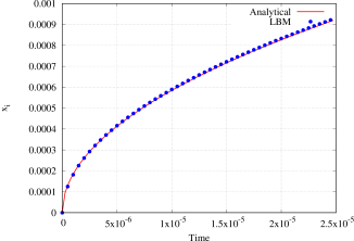
(a) Interface position $x_{i}(t)$ increasing with time because of precipitation process: the interface moves towards positive values of $x$.

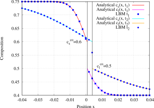
(b) Compositions of solid and liquid w.r.t $x$ at $t_{1}=2.5\times 10^{-5}$ and $t_{2}=5\times 10^{-4}$. The two vertical lines (black) indicate the interface positions $x_{i}(t_{1})$ (close to 0) and $x_{i}(t_{2})$. Zoom between $[-0.04,\,0.04]$. The $L^{2}$-errors are $4.8\times 10^{-3}$ for $t_{1}$ and $t_{2}$.

Figure 1: Analytical solutions Eqs. (52a)–(52c) (lines) compared to LBM (symbols) for one case of precipitation with $D_{s}=0.9$ and $D_{l}=1$. The system is initialized with an interface located at $x=0$. The solid and liquid are respectively on left- and right-side.

In [52], the solutions are derived for a ternary case. For binary case, the transcendental equation reduces to:

$$-\frac{1}{2}\alpha\Delta m{}^{2} =\Delta\overline{f}^{min}\left[u_{s}(-\alpha)+u_{l}(\alpha)\right]+$$

$$\qquad\Delta m\left[\left(m_{s}-c_{s}^{\infty}\right)u_{s}(-\alpha)+\right.$$

$$\qquad\qquad\left.\left(m_{l}-c_{l}^{\infty}\right)u_{l}(\alpha)\right]$$ (51a)

where the function $u_{\Phi}(\alpha)$ is defined by

$$u_{\Phi}(\alpha)=\sqrt{\frac{D_{\Phi}}{\pi}}\frac{e^{-\alpha^{2}/4D_{\Phi}}}{\text{erfc}\left(\alpha/2\sqrt{D_{\Phi}}\right)}\quad\text{for }\Phi=s,\,l$$ (51b)

The compositions far from the interface are $c_{s}^{\infty}=0.75$ and $c_{l}^{\infty}=0.4$. For $m_{s}=0.2$, $m_{l}=0.1$, $\Delta m=0.1$ and $\Delta\overline{f}^{min}=0.04$, the root of the transcendental equation is $\alpha=0.184841$. The three solutions are the interface position $x_{i}(t)$, the composition of solid $c_{s}(x,\,t)$ and the composition of liquid $c_{l}(x,\,t)$. The interface position writes as a function of $\alpha$ and $t$:

$$x_{i}(t)=\alpha\sqrt{t}$$ (52a)

Since $\alpha>0$, the interface moves from $x_{i}(0)=0$ towards positive values of $x$, meaning that a precipitation process occurs. The two analytical solutions in the solid and the liquid write:

$$c_{s}^{as}(x,\,t) =c_{s}^{\infty}+(c_{s}^{co}-c_{s}^{\infty})\frac{\text{erfc}\left[-x/2\sqrt{D_{s}t}\right]}{\text{erfc}\left[-\alpha/2\sqrt{D_{s}}\right]}$$ (52b)

$$c_{l}^{as}(x,\,t) =c_{l}^{\infty}+(c_{l}^{co}-c_{l}^{\infty})\frac{\text{erfc}\left[x/2\sqrt{D_{l}t}\right]}{\text{erfc}\left[\alpha/2\sqrt{D_{l}}\right]}$$ (52c)

where Eq. (52b) is defined for $x\in[-L_{x},\,x_{i}(t)[$ and Eq. (52c) for $x\in]x_{i}(t)],\,L_{x}]$. On the whole domain, the composition $c$ is discontinuous at interface $x_{i}(t)$, of value $c_{s}^{co}=0.6$ on solid side and $c_{l}^{co}=0.5$ on liquid side. From those values, each profile of composition diffuses until $c_{s}^{\infty}$ for $x\rightarrow-L_{x}$ and $c_{l}^{\infty}$ for $x\rightarrow L_{x}$.

The simulations are performed without anti-trapping current. The interpolation of diffusion coefficients is simply done by $\mathcal{D}(\phi)=\phi D_{l}+(1-\phi)D_{s}$. In $\phi$-equation the parameters are $M_{\phi}=1.2$, $W=1.2\times 10^{-3}$ and $\lambda^{\star}=277$. The comparisons between the analytical solutions and the LBM simulation are presented on Fig. 1. As expected from the theory, the interface position $x_{i}(t)$ is an increasing function of time (Fig. 1a). On the profiles of composition (Fig. 1b), the jump on each side of the interface is also well-reproduced by the numerical model. The coexistence values $c_{s}^{co}=0.6$ and $c_{l}^{co}=0.5$ remain the same at two times $t_{1}=2.5\times 10^{-5}$ and $t_{2}=5\times 10^{-4}$. The LBM simulations fit perfectly with the analytical solutions.

The two solutions Eqs. (52b)–(52c) can be easily expressed in terms of chemical potential $\overline{\mu}_{s}^{as}(x,\,t)$ and $\overline{\mu}_{l}^{as}(x,\,t)$. For instance, we add $-m_{s}$ on both sides of Eq. (52b) and add $m_{s}-m_{s}$ inside the term $(c_{s}^{co}-c_{s}^{\infty})$. Thanks to Eqs. (24a)–(24b) we obtain $(c_{s}^{co}-c_{s}^{\infty})\equiv(\overline{\mu}^{eq}-\overline{\mu}_{s}^{\infty})$ for solid and $(c_{l}^{co}-c_{l}^{\infty})\equiv(\overline{\mu}^{eq}-\overline{\mu}_{l}^{\infty})$ for liquid. When expressed in terms of chemical potential, the solution does not present a jump at interface $x_{i}(t)$. The single value is $\overline{\mu}^{eq}$ and each profile diffuse from that value until $\overline{\mu}_{s}^{\infty}$ when $x\rightarrow-L_{x}$ (solid) and $\overline{\mu}_{l}^{\infty}$ when $x\rightarrow L_{x}$ (liquid). The next section presents a validation using $\overline{\mu}$ as main variable for discussing the analogy with temperature and comparing with solidification problems.

4.2 Validation with $D_{s}=0$: effect of anti-trapping current

The analytical solution of the one-sided diffusion is presented in [51, Sec. 12-1]. Now a direct analogy is done between the temperature of that reference and the chemical potential of our model. The two solutions are $x_{i}(t)$, the interface position, and $\overline{\mu}_{l}^{as}(x,\,t)$ the chemical potential of liquid. The chemical potential of solid is set equal to the equilibrium value $\overline{\mu}^{eq}=0.4$. Its value remains constant during the simulation because $D_{s}=0$. The transcendental equation of that problem writes:

$$\alpha e^{\alpha^{2}}\text{erfc}(\alpha)+\frac{(\overline{\mu}^{eq}-\overline{\mu}_{l}^{\infty})}{(c_{s}^{co}-c_{l}^{co})\sqrt{\pi}}=0$$ (53)

where $\alpha$ is the root of this equation, and $\overline{\mu}_{l}^{\infty}$ is the value of chemical potential far from the interface. By analogy with problems of phase change (solidification or melting), the equilibrium chemical potential $\overline{\mu}^{eq}$ plays the role of melting temperature. The term $\Delta c^{co}=c_{s}^{co}-c_{l}^{co}$ can be compared to the latent heat. For phase change problems, that quantity is released (resp. absorbed) at interface during solidification (resp. melting). Here for our convention $c_{s}^{co}>c_{l}^{co}$, the quantity $\Delta c^{co}$ is released at interface during dissolution and absorbed during precipitation. Finally, the quantity $\chi=1$ plays the role of specific heat.

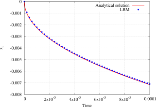
(a) Interface position $x_{i}(t)$ decreasing with time because of dissolution process: the interface moves towards negative values of $x$.

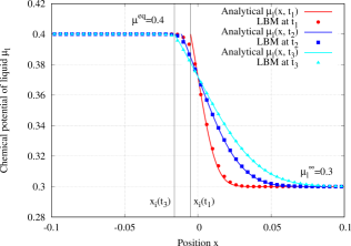
(b) Chemical potential $\overline{\mu}_{l}$ w.r.t. $x$ for three times $t_{1}=5\times 10^{-5}$ (red), $t_{2}=2.5\times 10^{-4}$ (blue) and $t_{3}=5\times 10^{-4}$ (cyan). The $L^{2}$-errors decrease with time: 1.6$\times 10^{-3}$ for $t_{1}$, 7.2$\times 10^{-4}$ for $t_{2}$ and 5.4$\times 10^{-4}$ for $t_{3}$. The two vertical lines (black) indicate the interface positions at $x_{i}(t_{1})$ and $x_{i}(t_{3})$.

Figure 2: Analytical solutions Eqs. (54a), (54b), (55a) (lines) compared with LBM (symbols) for a case of dissolution with $D_{s}=0$ and $D_{l}=1$. The anti-trapping current $\boldsymbol{j}_{at}$ is considered in the simulation. The system is initialized with an interface located at $x=0$. The solid and liquid are respectively on left- and right-side.

In Eq. (53), the dissolution or precipitation processes can occur depending on the sign of second term. We keep $c_{s}^{co}=0.6$ and $c_{l}^{co}=0.5$ (i.e. $\Delta c^{co}>0$), and we set $\overline{\mu}_{l}^{\infty}=0.3$ meaning that $\overline{\mu}^{eq}-\overline{\mu}_{l}^{\infty}>0$. The root of this equation is equal to $\alpha=-0.357835$. The interface position $x_{i}(t)$ is a function of $\alpha$, $t$ and $D_{l}$ which writes:

$$x_{i}(t)=2\alpha\sqrt{D_{l}t}$$ (54a)

Since $\alpha<0$, the interface position moves from $x_{i}(0)=0$ towards negative values of $x$, meaning that a dissolution process occurs. The chemical potential of liquid is

$$\overline{\mu}_{l}^{as}(x,\,t)=\overline{\mu}_{l}^{\infty}+(\overline{\mu}^{eq}-\overline{\mu}_{l}^{\infty})\frac{\text{erfc}[x/2\sqrt{D_{l}t}]}{\text{erfc}(\alpha)}$$ (54b)

for $x\in]x_{i}(t),\,L_{x}]$. In the liquid, $\overline{\mu}_{l}^{as}(x,\,t)$ diffuses from the equilibrium value $\overline{\mu}^{eq}$ at the interface until $\overline{\mu}_{l}^{\infty}$ when $x\rightarrow L_{x}$. In the solid, the chemical potential $\overline{\mu}_{s}^{as}(x,\,t)$ is constant of value $\overline{\mu}^{eq}$ for $x\in[-L_{x},\,x_{i}(t)[$.

For LBM simulations, the parameters of $\phi$-equation are $W=5\times 10^{-3}$, $\lambda^{\star}=230$ and $M_{\phi}=1.2$. In $c$-equation, the diffusion is interpolated by $\mathcal{D}(\phi)=\phi D_{l}$ and the anti-trapping current is considered. The initial condition of composition is imposed by Eq. (50) with $c_{l}^{\infty}=\overline{\mu}_{l}^{\infty}+m_{l}=0.4$ and $c_{s}^{\infty}=\overline{\mu}_{s}^{\infty}+m_{s}=0.6$ with $m_{s}=0.2$ and $m_{l}=0.1$. The comparisons between the analytical solutions and the LBM simulation are presented in Fig. 2. Compared to the previous section, now the curve of the interface position decreases with time (Fig. 2a) because the dissolution process occurs. The results of LBM are in good agreement with the analytical solutions for three times $t_{1}=5\times 10^{-5}$, $t_{2}=2.5\times 10^{-4}$ and $t_{3}=5\times 10^{-4}$ (Fig. 2b).

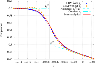
(a) Profiles of composition compared between LBM (symbols), analytical (dashed line) and semi-analytical solutions (solid lines). The $L^{2}$-errors are $3.6\times 10^{-3}$ with anti-trapping and $4.8\times 10^{-3}$ without.

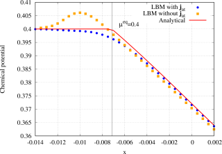
(b) Profiles of chemical potential compared between LBM (symbols) and analytical solution (line). The $L^{2}$-errors are $3.5\times 10^{-3}$ with anti-trapping and $6.8\times 10^{-3}$ without.

Figure 3: LB simulations with (dots) and without (squares) $\boldsymbol{j}_{at}$ in $c$-equation. Comparison on profiles of composition (Fig. 3a) and chemical potential (Fig. 3b). Zoom between $[-0.015,\,0.002]$ at $t=10^{-4}$.

The anti-trapping effect is compared on the profiles of composition and chemical potential (Fig. 3). For composition, the analytical solution can be derived from Eq. (54b) by adding $m_{l}$ on both sides and by adding and subtracting $m_{l}$ inside $(\overline{\mu}^{eq}-\overline{\mu}_{l}^{\infty})$. We obtain:

$$c_{l}^{as}(x,\,t)=c_{l}^{\infty}+(c_{l}^{co}-c_{l}^{\infty})\frac{\text{erfc}[x/2\sqrt{D_{l}t}]}{\text{erfc}(\alpha)}$$ (55a)

where $c_{l}^{co}=\overline{\mu}^{eq}+m_{l}=0.5$. In the solid phase, the composition is a constant of value $c_{s}(x,\,t)=\overline{\mu}^{eq}+m_{s}=0.6$ corresponding to its value of coexistence $c_{s}^{co}$. The compositions $c_{l}^{as}(x,\,t)$ and $c_{s}(x,\,t)$ are plotted with dashed lines on Fig. 3a.

The LBM simulations are carried out successively with and without anti-trapping current. The profiles of composition are reported on Fig. 3a at $t=10^{-4}$ (symbols). Without anti-trapping, the theory cannot provide a value of $\lambda^{\star}$ because the phase-field model is not strictly equivalent to the sharp interface one (see Section 2.4). Hence, the value of $\lambda^{\star}=500$ is chosen such as the displacement of the interface is close to the analytical solution. The simulation corresponds to the best fit that is possible to obtain when $D_{s}=0$ and $\boldsymbol{j}_{at}=\boldsymbol{0}$ in $c$-equation (squares on Fig. 3a). On that figure, the semi-analytical solution ($sas$) is plotted for comparison:

$$c^{sas}(\phi)=c_{l}^{as}(x,\,t)\phi(x,\,t)+c_{s}\left[1-\phi(x,\,t)\right]$$ (55b)

The $sas$-solution corresponds to an interpolation of $c_{l}^{as}(x,\,t)$ and $c_{s}$ with $\phi$. When $\boldsymbol{j}_{at}$ is not considered in $c$-equation, the compositions fit well far from the interface. However, inside the interface region, the compositions are over-estimated on the solid side whereas they are under-estimated on the liquid side. On the interval $[-L_{x},\,x_{i}(t)[$ (solid), the profile slightly oscillates above the composition of coexistence. That oscillation is more visible when we plot the chemical potential (Fig. 3b). That lack of accuracy slows down the displacement of interface compared to the analytical solution Eq. (54a).

5 Dissolution of porous medium: counter term effect

In Section 4, the initial conditions of $\phi$ and $c$ are defined by two hyperbolic tangent functions. Here, the phase-field is initialized with an input datafile which comes from the characterization of a 3D porous sample with X-ray tomography. The datafile contains $256\times 256\times 236$ rows with three indices of position ($x$, $y$ and $z$) and one additional index describing the solid (value 0) or the pore (value 255). For simulating the dissolution, we assume that the poral volume is filled with a solute of smaller composition than the coexistence composition of liquid. A two-dimensional slice of size $256\times 256$ has been extracted from the datafile and rescaled to $1024\times 1024$ nodes covering a square of size $[0,\,1]^{2}$ ($\delta x\simeq 9.76\times 10^{-4}$). The time-step of discretization is $\delta t=5\times 10^{-7}$. The type of all boundary conditions is zero flux.

For the parameters of $\phi$-equation, the diffusivity is $M_{\phi}=1.2$ and the interface width is set equal to $W=0.02$ (i.e. $\sim 20\delta x$). The value of coupling coefficient $\lambda^{\star}=230$ (corresponding to $\beta=0$) is computed by using Eq. (37) with values of $\mathscr{K}$, $\mathscr{F}$ and $\mathscr{I}=2/3$ defined in Tab. 3. For $c$-equation, the coexistence compositions of solid and liquid are respectively equal to $c_{s}^{co}=0.6$ and $c_{l}^{co}=0.5$ ($\Delta c^{co}=0.1$) and the chemical potential of equilibrium is $\overline{\mu}^{eq}=0.4$. The diffusion coefficients are zero in the solid ($D_{s}=0$) and one in the liquid ($D_{l}=1$). The anti-trapping current $\boldsymbol{j}_{at}$ is used in the simulations.

The phase-field is simply initialized at $t_{0}=0$ with two discontinuous values: for solid $\phi(\boldsymbol{x}_{s},\,t_{0})=\phi_{s}=0$ and for liquid $\phi(\boldsymbol{x}_{l},\,t_{0})=\phi_{l}=1$. The composition of the solid phase $c(\boldsymbol{x}_{s},\,t_{0})$ is set equal to the coexistence composition of solid $c_{s}^{co}$. For liquid, the initial condition is below its coexistence composition: $c(\boldsymbol{x}_{l},\,t_{0})=0.4<0.5$. Those initializations are presented on Fig. 4a for $\phi$ and Fig. 4b for $c$. On both figures, three squares are sketched for comparing the evolution of small pores which are enclosed inside the solid.

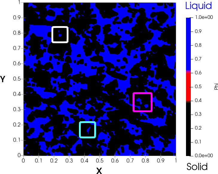
(a) Initialization of phase-field: for solid $\phi(\boldsymbol{x}_{s},\,t_{0})=\phi_{s}=0$ (black) and for liquid $\phi(\boldsymbol{x}_{l},\,t_{0})=\phi_{l}=1$ (blue).

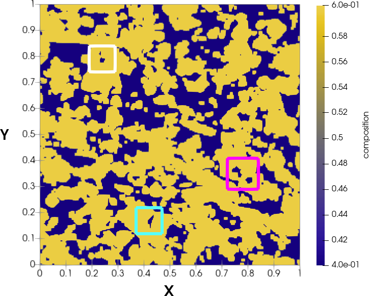
(b) Initialization of composition: for solid, the composition is set equal to the solid coexistence i.e. $c(\boldsymbol{x}_{s},\,t_{0})=c_{s}^{co}=0.6$ (yellow). For liquid $c(\boldsymbol{x}_{l},\,t_{0})=0.4$ (dark blue) i.e. below the composition of coexistence $c_{l}^{co}=0.5$.

Figure 4: Positions $\boldsymbol{x}_{s}$ and $\boldsymbol{x}_{l}$ of datafile used to define the initial conditions for $\phi$ (Fig. 4a) and $c$ (Fig. 4b). Three squares are sketched for comparing the evolution of small pores enclosed inside the solid.

With those initial conditions, the dissolution process occurs until the composition of the liquid phase is equal to $c_{l}^{co}$. Two simulations are compared. In the first one, the $\phi$-equation is Eq. (34) which accounts for the counter term $-M_{\phi}\kappa\bigl{|}\boldsymbol{\nabla}\phi\bigr{|}$. In the second one, the curvature-driven motion is possible because the $\phi$-equation is Eq. (33a). For both simulations, a diffuse interface replaces at first time-steps the initial discontinuity between the solid and liquid phases. The code ran 70 seconds on a single GPU (Volta 100) until the steady state is reached after $10^{4}$ time steps.

The results are presented in Fig. 5 for three times: $t_{1}=10^{2}\delta t$ (left), $t_{2}=10^{3}\delta t$ (middle) and $t_{f}=10^{4}\delta t$ (right). At first sight, the difference concerns the shapes of the solid phase at the end of simulations. When the counter term is considered, the interface is much more irregular (Fig. 5a-right) than that obtained without counter term (Fig. 5b-right). The reason is that, with counter term, the interface motion is only caused by differences of composition in liquid and solid. The dissolution occurs in isotropic way until the equilibrium is reached. Without counter term, the irregularities of solid disappear because of the curvature-driven motion. Finally, the shape of the solid phase is much smoother.

For both simulations, when the steady state is reached, the composition of liquid phase is equal to the coexistence composition of liquid $c(\boldsymbol{x}_{l},\,t_{f})=c_{l}^{co}$ (gray areas in the right figures of 5c and 5d). However, the composition inside the solid phase is different. When the curvature-driven motion is canceled, the composition $c(\boldsymbol{x}_{s},\,t_{f})$ is homogeneous of value $c_{s}^{co}$ (see Fig. 5c-right). When that motion is taken into account, the solid composition $c(\boldsymbol{x}_{s},\,t_{f})$ is heterogeneous as revealed by the presence of areas of composition lower than $c_{s}^{co}$ (gray areas inside squares in Fig. 5d-right). Those areas correspond to solid phases as confirmed by Fig. 5b-right.

That heterogeneity of composition is explained by the curvature-driven motion occurring when the counter term is not considered in $\phi$-equation. That interface motion makes disappear the small pores embedded in the solid phase. For instance at $t_{1}$, the small one inside the white square has disappeared (Fig. 5b-left) and the pore inside the cyan square has almost disappeared (red dot). That same pore has fully disappeared at $t_{2}$ (Fig. 5b-middle) and one of the two pores inside the magenta square has also disappeared. At last both of them have disappeared at $t_{f}$ (Fig. 5b-right). With counter term, all those pores still exist at the end of simulation (Fig. 5a-right).

With the curvature-driven motion a special area which is initially liquid ($\phi=1$) may become solid ($\phi=0$) even though the local composition $c(\boldsymbol{x}_{l},\,t)$ is not greater than $c_{l}^{co}$. That curvature motion acts like a precipitation process. For those areas, the diffusion coefficient changes from $D_{l}$ to $D_{s}=0$ meaning that the diffusion process does not occur anymore. The value of composition is “frozen” explaining why small islands of lower composition are embedded in the solid phase.

$t_{1}=2\times 10^{2}\delta t$	$t_{2}=10^{3}$$\delta t$	$t_{f}=10^{4}\delta t$

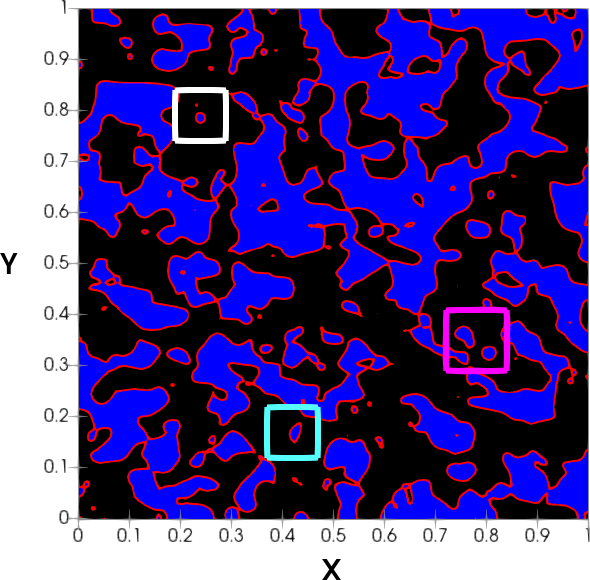
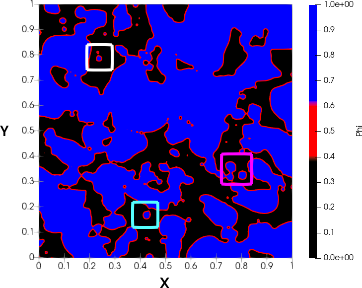
(a) Evolution of the phase-field when the counter term is considered in $\phi$-equation.

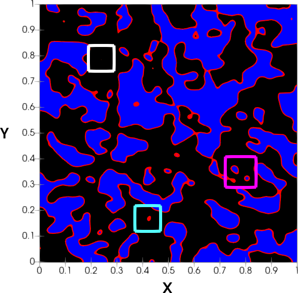
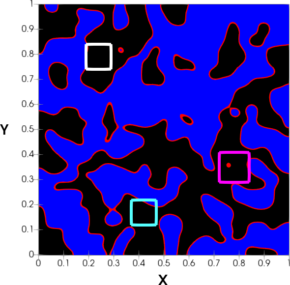
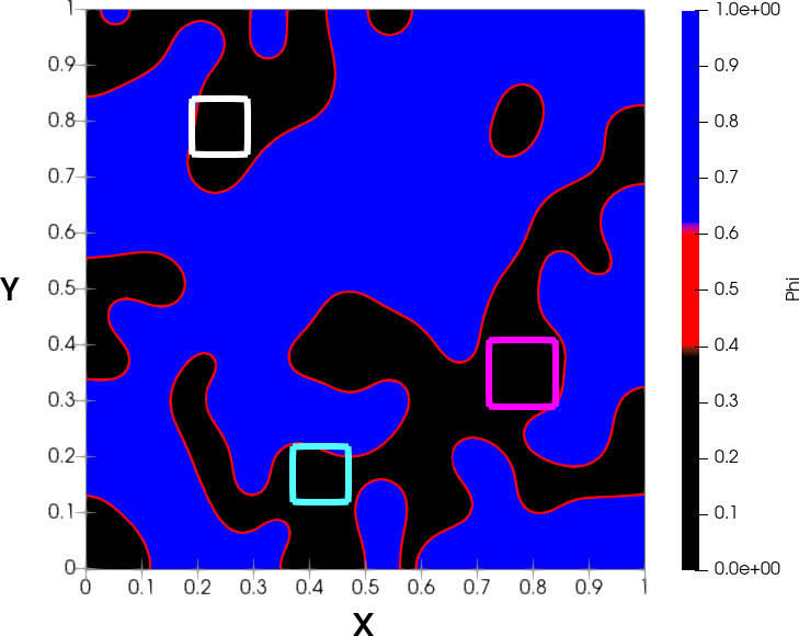
(b) Phase-field at same time steps without counter term. Because of the curvature-driven motion the final shape of solid is smoother and the small pores inside the squares have disappeared.

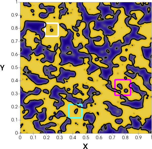
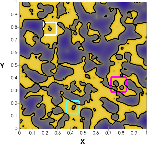
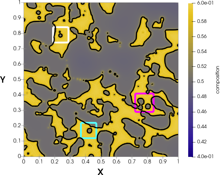
(c) Fields of composition at same time steps with counter term in $\phi$-equation. At final time the composition is homogeneous in the solid phase of value $c_{s}^{co}$.

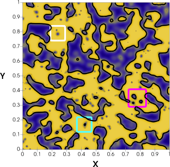
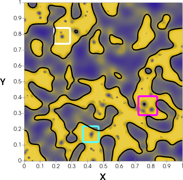
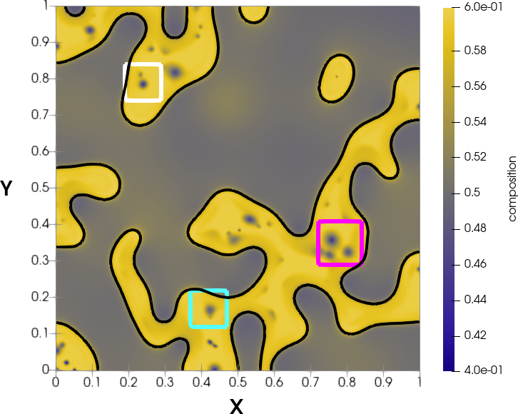
(d) Fields of composition without counter term at same time steps. The composition of solid is heterogeneous because the small pores have disappeared and the diffusion is zero. Several areas of smaller composition than $c_{s}^{co}$ are trapped in the solid phase (e.g. inside the squares).

Figure 5: Dissolution of porous medium simulated by a phase-field model based on the grand-potential. Snapshots of phase-field and composition at $t_{1}=2\times 10^{2}\delta t$ (left), $t_{2}=10^{3}\delta t$ (middle) and final time of simulation $t_{f}=10^{4}\delta t$ (right). Two simulations are carried out: in Figs. 5a and 5c the $\phi$-equation is Eq. (34) whereas in Figs. 5b and 5d the $\phi$-equation is Eq. (33a). The iso-contour $\phi=0.5$ (black line) is super-imposed on Figs. 5c and 5d.

An in-depth physical analysis is based on the Gibbs-Thomson condition Eq. (35c) i.e. $\overline{\mu}=\overline{\mu}^{eq}-d_{0}\kappa$ (with $\beta=0$). When two phases coexist, the interface will move towards the position where the chemical potential $\overline{\mu}$ is closer to $\overline{\mu}^{eq}$. In the first case, the counter term cancels the motion $d_{0}\kappa$ whereas in the second case that motion exists. In our simulations $\overline{\mu}(\boldsymbol{x}_{s},\,t)=\overline{\mu}^{eq}=0.4$ in the solid and $\overline{\mu}(\boldsymbol{x}_{l},\,t)=0.3$ in the liquid. For small pores trapped in the solid, the interface will move towards the liquid phase and the physical process acts like precipitation. The interface disappears because it is the unique way to reach the equilibrium value $\overline{\mu}^{eq}$. On the contrary, for outgrowths, the curvature is opposite and the interface will move towards the solid phase, dissolution occurs.

6 Conclusion

In this work we have presented a phase-field model of dissolution and precipitation. Its main feature lies in its derivation which is based on the functional of grand-potential $\Omega[\phi,\,\mu]$. In that theoretical framework, the phase-field $\phi$ and the chemical potential $\mu$ are the two main dynamical variables. In models based on free energy, $\phi$ and the composition $c$ are the two main variables. The benefits of using the grand-potential are twofold. First, for models based on free-energy, two additional conditions must be solved inside the diffuse zone in order to ensure the equality of chemical potential at interface. In grand-potential theory, it is not necessary because the model includes that assumption in its formulation. Second, the chemical potential is an intensive thermodynamic quantity like temperature so that many analogies can be done with solidification problems. Hence, the analytical solutions of the Stefan problem can be used for validation by comparing directly the temperature and the chemical potential. Besides, the matched asymptotic expansions can be directly inspired from those already performed for solidification problems. The phase-field model is composed of two PDEs. The first equation computes the evolution of the interface position $\phi$. The second one is a mixed formulation using the composition and chemical potential. Although that equation requires a closure relationship between $c$ and $\mu$, that formulation improves the mass conservation.

In many simulations of dissolution or precipitation, two main hypotheses are often considered. First, the interface is assumed to move because of chemical reactions, which is often considered by a kinetics of first-order. That assumption means that the curvature-driven motion is neglected in the Gibbs-Thomson condition. In the phase-field theory, that motion is always contained in the $\phi$-equation. In order to cancel it, a counter term $-M_{\phi}\kappa\bigl{|}\boldsymbol{\nabla}\phi\bigr{|}$ must be added in $\phi$-equation. The second hypothesis is the diffusion that is neglected in the solid phase. In that case, the anti-trapping current $\boldsymbol{j}_{at}$ must be considered in $c$-equation. Those two terms are not contained in the functional of grand-potential, they are added for phenomenological reasons. Without them, the phase-field model is not equivalent to the sharp interface model because several spurious terms arise from the matched asymptotic expansions.

The model has been implemented with lattice Boltzmann schemes in the LBM_saclay code. The one-dimensional validations have been carried out with two analytical solutions of the Stefan problem. The test cases present one process of precipitation with $D_{s}\simeq D_{l}$ and another one of dissolution for $D_{s}=0$. The first one is performed without anti-trapping and compares the profiles of composition. The jump of composition is well-reproduced by the model at interface. The diffusive behavior is also perfectly fitted for each phase. The second test emphasizes the analogy with problems of solidification (or melting) where the equilibrium chemical potential $\mu^{eq}$ plays the role of melting temperature and $\Delta c^{co}$ is compared to the latent heat. For that test, the use of anti-trapping current avoids the oscillations of algorithm and improves the accuracy of composition profiles.

Finally, the numerical model has been applied for simulating the dissolution process of a porous medium. The rock sample has been characterized by X-ray microtomography. The datafile has been used for defining the initial conditions for $\phi$ and $c$. Two simulations have compared the impact of counter term on the shape of solid. When the counter term is not considered in $\phi$-equation, the curvature-driven motion makes disappear small areas of liquid trapped inside the solid phase. The main consequence of that effect, acting like precipitation, is the heterogeneity of composition inside the solid phase. When the counter term is taken into account, the solid/liquid interface is much more irregular and the composition is homogeneous inside the solid phase.

The grand-potential densities $\omega_{\Phi}$ of each phase are defined by the Legendre transform of free energy densities $f_{\Phi}$. In this work, the main assumption is that $f_{s}$ and $f_{l}$ are defined by two parabolas with identical curvature $\epsilon_{s}=\epsilon_{l}$. That hypothesis simplifies the link between the thermodynamic parameters $m_{\Phi}$, $\epsilon_{\Phi}$ and $\overline{f}_{\Phi}^{min}$and the properties of equilibrium i.e. the coexistence compositions $c_{s}^{co}$, $c_{l}^{co}$, and the equilibrium chemical potential $\mu^{eq}$. Nevertheless, for real materials the thermodynamics does not fulfill necessarily that condition. An in-depth study with $\epsilon_{s}\neq\epsilon_{l}$ is planned for future work for binary and ternary mixtures.

Appendix A Matched asymptotic expansions

The starting point of this Appendix is the phase-field model composed of Eqs. (33a)–(33c). The analysis is performed into two main stages. First, the whole computational domain is divided into two regions. The first region is located far from the interface (bulk phases) and called the “outer domain”. The second region is the diffuse interface and called the “inner domain”. In A.1, we define the dimensionless variables and the matching conditions between both regions. Next, we present the analysis of the outer domain in A.2 and the inner domain in A.3. Finally a discussion is carried out in A.4 to remove the error terms.

A.1 Main definitions

A.1.1 Outer domain and inner domain

The unknown are $\phi^{out}$, $\mu^{out}$, $c^{out}$ for the outer domain, and $\phi^{in}$, $\mu^{in}$, $c^{in}$ for the inner domain. They are expanded as power of a small parameter ${\displaystyle\varepsilon\ll 1}$:

$$\phi^{out} \simeq\phi_{0}^{out}+\varepsilon\phi_{1}^{out}+\varepsilon^{2}\phi_{2}^{out}, \phi^{in} \simeq\phi_{0}^{in}+\varepsilon\phi_{1}^{in}+\varepsilon^{2}\phi_{2}^{in}$$

$$c^{out} \simeq c_{0}^{out}+\varepsilon c_{1}^{out}+\varepsilon^{2}c_{2}^{out}, c^{in} \simeq c_{0}^{in}+\varepsilon c_{1}^{in}+\varepsilon^{2}c_{2}^{in}$$

$$\mu^{out} \simeq\mu_{0}^{out}+\varepsilon\mu_{1}^{out}+\varepsilon^{2}\mu_{2}^{out}, \mu^{in} \simeq\mu_{0}^{in}+\varepsilon\mu_{1}^{in}+\varepsilon^{2}\mu_{2}^{in}$$

The small parameter of expansions is defined by $\varepsilon=W/d_{0}$, where $d_{0}=W/(\alpha\lambda)$ is the capillary length, and $\alpha$ is a parameter to be determined. The two coefficients $D_{l}$ and $d_{0}$ define a characteristic speed $v_{c}=D_{l}/d_{0}=\varepsilon D_{l}/W$, and a characteristic time $t_{c}=d_{0}^{2}/D_{l}=d_{0}/v_{c}$. For the expansions, we also assume $1/\kappa\sim d_{0}$ i.e. ${\displaystyle W\kappa\sim\varepsilon}$. In the phase-field equation, the coefficient $\lambda$ is replaced by $\varepsilon/\alpha$. Finally, we define the following dimensionless quantities: the interface speed $\bar{v}_{n}=v_{n}/v_{c}$, the interface curvature $\bar{\kappa}=d_{0}\kappa$, the time $\bar{t}=t/t_{c}$, the spatial coordinate $\bar{\boldsymbol{x}}=\boldsymbol{x}/d_{0}$, and the dimensionless diffusivity $\bar{D}=D_{l}/M_{\phi}$. Finally $q_{s}=D_{s}/D_{l}$ is the ratio of diffusion coefficients.

For each domain, the model is re-written with the curvilinear coordinates $r$ and $s$, where $r$ is the signed distance to the level line $\phi=0.5$, and $s$ the arc length along the interface. The dimensionless coordinates are also defined by: $\eta=r/d_{0}$ and $\overline{s}=s/d_{0}$. The spatial operators (divergence, gradient, laplacian) and the time derivatives are also expressed in this new system of coordinates, and next expanded in power of $\varepsilon$. Finally, the terms of same order are gathered and the solutions of all orders can be calculated with appropriate boundary conditions: the “matching conditions”.

A.1.2 Matching conditions

The matching conditions are established by comparing the limits of inner variables far from the interface with the limits of outer variables near the interface. For that purpose we define $\xi=r/W$, a “stretched” normal coordinate in the inner region. Let us notice that the curvilinear coordinates $r$ and $s$ have been made dimensionless by introducing $\eta=r/d_{0}$ and $\overline{s}=s/d_{0}$ in the outer domain, we observe that $\eta/\xi=\varepsilon\ll 1$. This motivates us to compare the limits of inner variables when $\xi\rightarrow\pm\infty$ with the limits of outer variables when $\eta\rightarrow 0^{\pm}$. For the phase-fields $\phi_{0}^{in}$ and $\phi_{0}^{out}$, we define the matching conditions:

$$\underset{\xi\rightarrow+\infty}{\lim}\phi_{0}^{in}=\underset{\eta\rightarrow 0^{+}}{\lim}\phi_{0}^{out}\quad\text{and}\quad\underset{\xi\rightarrow-\infty}{\lim}\phi_{0}^{in}=\underset{\eta\rightarrow 0^{-}}{\lim}\phi_{0}^{out}$$

For the chemical potentials $\mu_{j}^{in}$ and $\mu_{j}^{out}$ ($0\leq j\leq 2$), the matching conditions are:

$$\underset{\xi\rightarrow\pm\infty}{\lim}\mu_{0}^{in} =\mu_{0}^{out}(0^{\pm})$$

$$\underset{\xi\rightarrow\pm\infty}{\lim}\mu_{1}^{in} =\mu_{1}^{out}(0^{\pm})+\partial_{\eta}\mu_{0}^{out}(0^{\pm})\xi$$

$$\underset{\xi\rightarrow\pm\infty}{\lim}\partial_{\xi}\mu_{2}^{in} =\partial_{\eta}\mu_{1}^{out}(0^{\pm})+\partial_{\eta\eta}^{2}\mu_{0}^{out}(0^{\pm})\xi$$

where $\mu_{j}^{out}(0^{\pm})=\lim_{\eta\rightarrow 0^{\pm}}\mu_{j}^{out}$ for $j=0,\,1$ and $\partial_{\eta}\mu_{0}^{out}(0^{\pm})=\lim_{\eta\rightarrow 0^{\pm}}\partial_{\eta}\mu_{0}^{out}$.

A.2 Analysis of outer domain

In the outer domain, the use of curvilinear coordinates is not necessary because the region is far from the interface. Thus, the model is written with the dimensionless cartesian coordinates $\overline{\boldsymbol{x}}$, the dimensionless time $\overline{t}$ and the parameter of expansion $\varepsilon$. The model writes:

$$\bar{D}\varepsilon^{2}\partial_{\bar{t}}\phi^{out} =\varepsilon^{2}\boldsymbol{\bar{\nabla}}^{2}\phi^{out}-\omega_{dw}^{\prime}(\phi^{out})-\frac{\varepsilon}{\alpha}\partial_{\phi}\omega^{p}(\phi^{out},\mu^{out})$$

$$\partial_{\bar{t}}c =\boldsymbol{\bar{\nabla}}\cdot\left[q(\phi^{out})\boldsymbol{\bar{\nabla}}\mu^{out}-\boldsymbol{j}_{at}(\phi^{out})\right]$$ (56)

where the notation $\omega^{p}=p(\phi)\omega_{l}(\mu)+[1-p(\phi)]\omega_{s}(\mu)$ and $\boldsymbol{j}_{at}(\phi^{out})=-a(\phi^{out})\Delta c^{co}\partial_{\bar{t}}\phi^{out}\boldsymbol{n}$ with the normal vector $\boldsymbol{n}=\boldsymbol{\bar{\nabla}}\phi^{out}/\left|\boldsymbol{\bar{\nabla}}\phi^{out}\right|$. The expansions of $\phi$-equation write for each order:

$$\mathcal{O}(1):\quad 0=\omega_{dw}^{\prime}(\phi_{0}^{out})$$ (57a)

$$\mathcal{O}(\varepsilon):\quad 0=\omega_{dw}^{\prime\prime}(\phi_{0}^{out})\phi_{1}^{out}+\alpha^{-1}\partial_{\phi}\omega^{p}(\phi_{0}^{out},\mu_{0}^{out})$$ (57b)

$$\mathcal{O}(\varepsilon^{2}):\quad 0=\bar{D}\varepsilon^{2}\partial_{\bar{t}}\phi_{0}^{out}-\boldsymbol{\bar{\nabla}}^{2}\phi_{0}^{out}+\omega_{dw}^{\prime\prime\prime}(\phi_{0}^{out})\phi_{2}^{out}$$

$$+\frac{1}{2}\omega_{dw}^{\prime\prime}(\phi_{0}^{out})(\phi_{1}^{out})^{2}+\frac{1}{\alpha}\partial_{\phi\phi}^{2}\omega^{p}(\phi_{0}^{out},\mu_{0}^{out})\phi_{1}^{out}$$

$$\qquad\qquad+\alpha^{-1}\partial_{\phi\mu}^{2}\omega^{p}(\phi_{0}^{out},\mu_{0}^{out})\mu_{1}^{out}$$ (57c)

According to Eq. (57a), $\omega_{dw}(\phi_{0}^{out})$ takes a minimal value in the outer domain, i.e. $\phi_{0}^{out}$ is either equal to $\phi_{s}=0$ or $\phi_{l}=1$. In addition, $p(\phi)$ must be chosen such that its derivatives vanish in the bulk phases. Then Eq. (57b) becomes simply $\omega_{dw}^{\prime\prime}(\phi_{0}^{out})\phi_{1}^{out}=0$, implying $\phi_{1}^{out}=0$. Similarly, Eq. (57c) simplifies to $\omega_{dw}^{\prime\prime}(\phi_{0}^{out})\phi_{2}^{out}=0$ involving $\phi_{2}^{out}=0$. Finally, the analysis of $\phi$-equation in the outer domain yields

$$\phi_{0}^{out}=\phi_{\Phi}\quad\text{and}\quad\phi_{1}^{out}=\phi_{2}^{out}=0\quad\text{for}\,\,\,\Phi=s,\,l$$ (58)

We can complete the matching conditions with the additional relation $\lim_{\xi\rightarrow\pm\infty}\phi_{j}^{in}=0$ for $j\geq 1$. Because of Eq. (58), the term $\partial_{\overline{t}}\phi^{out}$ is null in Eq. (56), and the $c$-equation simplifies to:

$$\partial_{\bar{t}}c=\boldsymbol{\bar{\nabla}}\cdot\left[q(\phi_{\Phi})\boldsymbol{\bar{\nabla}}\mu^{out}\right]\quad\text{for}\,\,\,\Phi=s,\,l$$ (59)

The analysis of the outer domain recovers the standard diffusion equation Eq. (59) with a constant phase-field Eq. (58) for each bulk phase.

A.3 Analysis of inner domain

Now we focus on the analysis of the inner domain. After expansions of each PDE (A.3.1), the solutions are calculated order-by-order and used to derive the interface conditions (A.3.2–A.3.6).

A.3.1 Expanded equations

The expansions of $\phi$-equation and $c$-equation write:

$$\mathcal{O}(1):\quad \partial_{\xi\xi}^{2}\phi_{0}^{in}-\omega_{dw}^{\prime}(\phi_{0}^{in}) =0$$ (60a)

$$\mathcal{O}(\varepsilon):\quad \partial_{\xi\xi}^{2}\phi_{1}^{in}-\omega_{dw}^{\prime\prime}(\phi_{0}^{in})\phi_{1}^{in} =-\left(\bar{D}\bar{v}_{n}+\bar{\kappa}\right)\partial_{\xi}\phi_{0}+\alpha^{-1}\partial_{\phi}\omega^{p}\left(\phi_{0}^{in},\mu_{0}^{in}\right)$$ (60b)

$$\mathcal{O}(\varepsilon^{2}):\quad \partial_{\xi\xi}^{2}\phi_{2}^{in}-\omega_{dw}^{\prime\prime}(\phi_{0}^{in})\phi_{2}^{in} =(1/2)(\phi_{1}^{in})^{2}\omega_{dw}^{\prime\prime\prime}(\phi_{0}^{in})+\bar{D}\partial_{\overline{t}}\phi_{0}^{in}-\partial_{\overline{s}\overline{s}}^{2}\phi_{0}^{in}-(\bar{D}\bar{v}_{n}+\bar{\kappa})\partial_{\xi}\phi_{1}^{in}$$ (60c)

$$\qquad+\xi\bar{\kappa}^{2}\partial_{\xi}\phi_{0}^{in}+\alpha^{-1}\partial_{\phi\phi}^{2}\omega^{p}(\phi_{0}^{in},\mu_{0}^{in})\phi_{1}^{in}+\alpha^{-1}\partial_{\phi\mu}^{2}\omega^{p}(\phi_{0}^{in},\mu_{0}^{in})\mu_{1}^{in}$$

$$\mathcal{O}(1):\quad \partial_{\xi}\left[q(\phi_{0}^{in})\partial_{\xi}\mu_{0}^{in}\right] =0$$ (61a)

$$\mathcal{O}(\varepsilon):\quad \partial_{\xi}\left[q(\phi_{0}^{in})\partial_{\xi}\mu_{1}^{in}\right] =-\partial_{\xi}\left[\phi_{1}^{in}\partial_{\phi}q(\phi_{0}^{in})\partial_{\xi}\mu_{0}^{in}\right]-\bar{v}_{n}\partial_{\xi}c_{0}^{in}-\bar{\kappa}q(\phi_{0}^{in})\partial_{\xi}\mu_{0}^{in}+\partial_{\xi}\left[a(\phi_{0}^{in})\Delta c^{co}\bar{v}_{n}\partial_{\xi}\phi_{0}^{in}\right]$$ (61b)

$$\mathcal{O}(\varepsilon^{2}):\quad \partial_{\xi}\left[q(\phi_{0}^{in})\partial_{\xi}\mu_{2}^{in}\right] =\partial_{\overline{t}}c_{0}^{in}+\xi\bar{\kappa}^{2}q(\phi_{0}^{in})\partial_{\xi}\mu_{0}^{in}-\bar{v}_{n}\partial_{\xi}c_{1}^{in}-\bar{\kappa}q(\phi_{0}^{in})\partial_{\xi}\mu_{1}^{in}$$ (61c)

$$\qquad-\partial_{\overline{s}}\left[q(\phi_{0}^{in})\partial_{\overline{s}}\mu_{0}^{in}\right]-\bar{\kappa}\phi_{1}^{in}\partial_{\phi}q(\phi_{0}^{in})\partial_{\xi}\mu_{0}^{in}-\partial_{\xi}\left[\phi_{1}^{in}\partial_{\phi}q(\phi_{0}^{in})\partial_{\xi}\mu_{1}^{in}\right]$$

$$\qquad-\partial_{\xi}\left\{\left[\phi_{2}^{in}\partial_{\phi}q(\phi_{0}^{in})+(\phi_{1}^{in\,2}/2)\partial_{\phi\phi}^{2}q(\phi_{0}^{in})\right]\partial_{\xi}\mu_{0}^{in}\right\}+\Delta c^{co}\bar{\kappa}a(\phi_{0}^{in})\bar{v}_{n}\partial_{\xi}\phi_{0}^{in}$$

$$\qquad+\Delta c^{co}\partial_{\xi}\left[a(\phi_{0}^{in})\bar{v}_{n}\partial_{\xi}\phi_{1}^{in}+a^{\prime}(\phi_{0}^{in})\bar{v}_{n}\phi_{1}^{in}\partial_{\xi}\phi_{0}^{in}\right]$$

The closure equation writes (only $\mathcal{O}(1)$ is necessary):

$$\mathcal{O}(1): \qquad c_{0}^{in}=-\partial_{\mu}\omega^{h}(\phi_{0}^{in},\mu_{0}^{in})$$ (62)

In the rest of this section, the superscript “in” will be removed for all inner variables i.e. for $0\leq j\leq 2$ we note $\phi_{j}\equiv\phi_{j}^{in}$, $\mu_{j}\equiv\mu_{j}^{in}$ and $c_{j}\equiv c_{j}^{in}$. The superscript “out” is kept for the variables of outer domain.

A.3.2 Analysis of terms $\mathcal{O}(1)$

For $\phi$-equation, Eq. (60a) can be easily solved by using $\omega_{dw}$. At order zero, we obtain the hyperbolic tangent profile of the phase-field:

$$\phi_{0}(\xi)=\frac{1+\tanh(2\xi)}{2}$$ (63)

For $c$-equation, two successive integrations of Eq. (61a) yield $\partial_{\xi}\mu_{0}=A(\overline{s})/q(\phi_{0})$ and $\mu_{0}=B(\overline{s})+A(\overline{s})\int_{0}^{\xi}q^{-1}(\phi_{0})d\xi$. Both constants of integration $A$ and $B$ can depend on $\overline{s}$. We can see that $A=0$ is necessary because the integral does not converge when $\xi\rightarrow+\infty$ (because $q\rightarrow 1$ when $\xi\rightarrow+\infty$). Hence, $\mu_{0}$ depends only on the position along the interface $\overline{s}$, and the matching conditions yield:

$$\mu_{0}^{out}(0^{+})=\mu_{0}^{out}(0^{-})$$ (64)

i.e. the continuity of the chemical potential at order zero.

A.3.3 $\phi$-equation: analysis of terms $\mathcal{O}(\varepsilon)$

The Gibbs-Thomson condition at order zero arises from the analysis of terms $\mathcal{O}(\varepsilon)$ of $\phi$-equation. After multiplication of Eq. (60b) by $\partial_{\xi}\phi_{0}$ and integration wrt $\xi$ from $-\infty$ to $+\infty$, we obtain:

$$\int_{-\infty}^{+\infty}\mathcal{L}(\phi_{1})\partial_{\xi}\phi_{0}d\xi =-\left(\bar{D}\bar{v}_{n}+\bar{\kappa}\right)\int_{-\infty}^{+\infty}(\partial_{\xi}\phi_{0})^{2}d\xi+$$

$$\quad\frac{1}{\alpha}\int_{-\infty}^{+\infty}\partial_{\xi}\phi_{0}\partial_{\phi}\omega^{p}(\phi_{0},\mu_{0})d\xi$$ (65)

where we set $\mathcal{L}(\phi_{1})=\partial_{\xi\xi}^{2}\phi_{1}-\omega_{dw}^{\prime\prime}(\phi_{0})\phi_{1}$. The left-hand side (LHS) of Eq. (65) is integrated by parts (using $\mathcal{O}(1)$ phase field for the last equality), we find:

$$\int_{-\infty}^{+\infty}\partial_{\xi}\phi_{0}\mathcal{L}(\phi_{1})d\xi=-\int_{-\infty}^{+\infty}\partial_{\xi}\phi_{1}\mathcal{L}(\phi_{0})d\xi=0$$

In the right-hand side (RHS) of Eq. (65), the first integral is noted $\mathscr{I}=\int_{-\infty}^{+\infty}(\partial_{\xi}\phi_{0})^{2}d\xi=2/3$. The second integral can be calculated because $\mu_{0}$ is independent of $\xi$. Finally Eq. (65) becomes:

$$0=-(\bar{D}\bar{v}_{n}+\bar{\kappa})\mathscr{I}+\frac{1}{\alpha}\left[\omega_{l}(\mu_{0})-\omega_{s}(\mu_{0})\right]$$ (66)

Using the expression $\omega_{l}(\mu_{0})-\omega_{s}(\mu_{0})=-(c_{l}^{co}-c_{s}^{co})(\mu_{0}-\mu^{eq})$ and the definitions of $\overline{D}$, $\overline{v}_{n}$ and $\overline{\kappa}$, we obtain:

$$(\mu_{0}-\mu^{eq})\Delta c^{co}=-\frac{\mathscr{I}W}{\lambda}\kappa-\frac{\mathscr{I}W}{M_{\phi}\lambda}v_{n}$$ (67)

where $\Delta c^{co}=c_{l}^{co}-c_{s}^{co}$. We identify $d_{0}=\mathscr{I}W/\lambda$, meaning that $\alpha=1/\mathscr{I}$, and $\beta_{0}=d_{0}/M_{\phi}$.

Another useful result for simplifying the future analyses is the first-order phase-field $\phi_{1}$. The bilinear form $(\psi,\,\phi)\rightarrow\int\psi\mathcal{L}(\phi)$ is continuous and coercive where $\psi$ and $\phi$ are two functions vanishing at $+\infty$ and $-\infty$. This means that the operator $\mathcal{L}$ is invertible in this space. Combined with Eq. (66), this indicates that $\phi_{1}$ is determined by:

$$\phi_{1} =\frac{\Delta\omega(\mu_{0})}{\alpha}\mathcal{L}^{-1}\left[p^{\prime}(\phi_{0})-\frac{1}{\mathscr{I}}\partial_{\xi}\phi_{0}\right]$$

With the derivatives of $p(\phi)$ and $\phi_{0}$ defined in Tab 2 and $\mathscr{I}=2/3$, the term inside the brackets vanishes. The unique solution is $\phi_{1}=0$ meaning that all terms depending on $\phi_{1}$ in Eqs. (60c), (61b) and (61c) can be removed.

A.3.4 $c$-equation: analysis of terms $\mathcal{O}(\varepsilon)$

The Stefan condition at order zero arises from the analysis of terms $\mathcal{O}(\varepsilon)$ of $c$-equation. However, the analysis also reveals two spurious terms for the chemical potential: the chemical potentials of first-order $\mu_{1}^{out}(0^{+})$ and $\mu_{1}^{out}(0^{-})$ are not identical on both sides of the interface.

We start with a simplification of $c$-equation Eq. (61b) with the previous result $\partial_{\xi}\mu_{0}=0$:

$$\partial_{\xi}\left[q(\phi_{0})\partial_{\xi}\mu_{1}\right]=-\bar{v}_{n}\partial_{\xi}c_{0}+\partial_{\xi}\left[\Delta c^{co}a(\phi_{0})\bar{v}_{n}\partial_{\xi}\phi_{0}\right]$$

After one integration, we obtain:

$$q(\phi_{0})\partial_{\xi}\mu_{1}=-\bar{v}_{n}c_{0}+A+\Delta c^{co}a(\phi_{0})\bar{v}_{n}\partial_{\xi}\phi_{0}$$ (68)

Considering the limit $\xi\rightarrow-\infty$, the integration constant $A$ is found equal to $A=\Lambda_{s}+\bar{v}_{n}c_{s}(\mu_{0})$ where $\Lambda_{s}=q_{s}\partial_{\eta}\mu_{0}^{out}(0^{-})$. The closure relation Eq. (62) writes $c_{0}=h(\phi_{0})c_{l}(\mu_{0})+\left[1-h(\phi_{0})\right]c_{s}(\mu_{0})$. Eq. (68) becomes

$$\partial_{\xi}\mu_{1}=\frac{1}{q(\phi_{0})}\left[-\bar{v}_{n}h(\phi_{0})\Delta c_{0}+\Lambda_{s}+\Delta c^{co}a(\phi_{0})\bar{v}_{n}\partial_{\xi}\phi_{0}\right]$$ (69)

where $\Delta c_{0}=c_{l}(\mu_{0})-c_{s}(\mu_{0})$. Because of the choice of free energies, we also have $\Delta c_{0}=\Delta c^{co}$ (see Eqs. (24a)-(24b)). Integrating once again from $0$ to $\xi$, we obtain

$$\mu_{1} =\Upsilon-\bar{v}_{n}\Delta c_{0}\int_{0}^{\xi}\frac{h(\phi_{0})}{q(\phi_{0})}$$

$$\qquad+\Lambda_{s}\int_{0}^{\xi}\frac{1}{q(\phi_{0})}+\bar{v}_{n}\int_{0}^{\xi}\frac{a(\phi_{0})\Delta c^{co}\partial_{\xi}\phi_{0}}{q(\phi_{0})}$$ (70)

where $\Upsilon$ is a constant of integration that will be determined in A.3.5. Now the matching conditions are used when $\xi\rightarrow\pm\infty$. When $\xi\rightarrow+\infty$, we ensure the convergence of the first two integrals by adding $+1-1$ i.e. the first integral considered is $\int_{0}^{\xi}h(\phi_{0})/q(\phi_{0})+1-1$ and the second one is $\Lambda_{s}\int_{0}^{\xi}q^{-1}(\phi_{0})+1-1$. This yields:

$$\mu_{1}^{out}(0^{+})+\partial_{\eta}\mu_{0}^{out}(0^{+})\xi=\Upsilon+\Delta c_{0}\bar{v}_{n}\mathscr{F}_{l}\qquad\quad$$

$$-\bar{v}_{n}\Delta c_{0}\xi+q_{s}\partial_{\eta}\mu_{0}^{out}(0^{-})[\mathscr{G}_{l}+\xi]$$ (71a)

$$\mu_{1}^{out}(0^{-})+\partial_{\eta}\mu_{0}^{out}(0^{-})\xi=\Upsilon+\Delta c_{0}\bar{v}_{n}\mathscr{F}_{s}\qquad\quad$$

$$+q_{s}\partial_{\eta}\mu_{0}^{out}(0^{-})[\mathscr{G}_{s}+(\xi/q_{s})]$$ (71b)

where $$\mathscr{F}_{l} \mathscr{F}_{s} \mathscr{G}_{l} \mathscr{G}_{s} \xi$$, , and are four integrals which are defined in Tab. 3. In Eqs. (71a)-(71b), the -terms are considered separately and gathered in one additional equation. The three equations write:

$$\mu_{1}^{out}(0^{+}) =\Upsilon+\bar{v}_{n}\Delta c_{0}\mathscr{F}_{l}+q_{s}\partial_{\eta}\mu_{0}^{out}(0^{-})\mathscr{G}_{l}$$ (72a)

$$\mu_{1}^{out}(0^{-}) =\Upsilon+\bar{v}_{n}\Delta c_{0}\mathscr{F}_{s}+q_{s}\partial_{\eta}\mu_{0}^{out}(0^{-})\mathscr{G}_{s}$$ (72b)

$$\partial_{\eta}\mu_{0}^{out}(0^{+}) =-\bar{v}_{n}\Delta c_{0}+q_{s}\partial_{\eta}\mu_{0}^{out}(0^{-})$$ (72c)

The last relationship Eq. (72c) is the Stefan condition at order zero:

$$\partial_{\eta}\mu_{0}^{out}(0^{+})-q_{s}\partial_{\eta}\mu_{0}^{out}(0^{-}) =-\bar{v}_{n}\Delta c_{0}$$ (73)

Eq. (72a) minus Eq. (72b) yields the jump of the first-order chemical potential:

$$\mu_{1}^{out}(0^{+})-\mu_{1}^{out}(0^{-})=\bar{v}_{n}\Delta c_{0}\Delta\mathscr{F}+q_{s}\partial_{\eta}\mu_{0}^{out}(0^{-})\Delta\mathscr{G}$$ (74)

where $\Delta\mathscr{F}=\mathscr{F}_{l}-\mathscr{F}_{s}$ and $\Delta\mathscr{G}=\mathscr{G}_{l}-\mathscr{G}_{s}$. The first-order chemical potentials are not the same on both side of the interface. The discontinuity contains two terms proportional to $\bar{v}_{n}\Delta c_{0}$ and $q_{s}\partial_{\eta}\mu_{0}^{out}(0^{-})$.

A.3.5 $\phi$-equation: analysis of terms $\mathcal{O}(\varepsilon^{2})$

The analysis of terms $O(\varepsilon^{2})$ of $\phi$-equation reveals that the discontinuity of the first-order chemical potential adds an error term in the Gibbs-Thomson condition. Since $\phi_{1}=0$ and $\phi_{0}$ does not depend on $\bar{t}$ and $\overline{s}$, Eq. (60c) simplifies to:

$$\partial_{\xi\xi}^{2}\phi_{2}-\omega_{dw}^{\prime\prime}(\phi_{0})\phi_{2} =\alpha^{-1}\partial_{\phi\mu}^{2}\omega^{p}(\phi_{0},\mu_{0})\mu_{1}+\xi\bar{\kappa}^{2}\partial_{\xi}\phi_{0}$$

We use the same method applied to $\phi$-eq of order $\mathcal{O}(\varepsilon)$: the LHS is noted $\mathcal{L}(\phi_{2})$ and we multiply the two sides by $\partial_{\xi}\phi_{0}$ before integrating over $\xi$ varying from $-\infty$ to $+\infty$:

$$\int_{-\infty}^{\infty}\partial_{\xi}\phi_{0}\mathcal{L}(\phi_{2}) d\xi=\alpha^{-1}\int_{-\infty}^{+\infty}\partial_{\xi}\phi_{0}\partial_{\phi\mu}^{2}\omega^{p}(\phi_{0},\mu_{0})\mu_{1}d\xi$$

$$\qquad+\int_{-\infty}^{\infty}\bar{\kappa}^{2}\xi(\partial_{\xi}\phi_{0})^{2}d\xi$$ (75)

With the same arguments as the $\mathcal{O}(\varepsilon)$-equation, the LHS of Eq. (75) is null. The last integral on the RHS vanishes because the integrand is odd. Eq. (75) is reduced to:

$$\int_{-\infty}^{+\infty}\left[\partial_{\xi}\phi_{0}\partial_{\phi\mu}^{2}\omega^{p}(\phi_{0},\mu_{0})\mu_{1}\right]d\xi=0$$ (76)

From this point, the analysis is straightforward. Comparatively, during the analysis of a KKS-type formulation of the model (like in [17, Appendix A]), a similar integral would have been obtained, but with the interpolation of grand potentials $\omega^{p}$ which is replaced by the free energy of an interpolation of compositions. A lengthy analysis involving the closure equation 62 expanded at first-order would have been required to get to the same point. Here, the use of the grand-potential formulation significantly simplifies the analysis. It can also be noted that such a simplification has already been used for the $\mathcal{O}(\varepsilon)$-terms of $\phi$-equation in Sec. A.3.3 because the integration of $\partial_{\xi}\phi_{0}\partial_{\phi}\omega^{p}(\phi_{0},\,\mu_{0})$ is much easier than $\partial_{\xi}\phi_{0}\partial_{\phi}f(\phi_{0},\,c_{0})$ (since $\mu_{0}$ is constant and not $c_{0}$). In Eq. (76), we replace $\mu_{1}$ by its expression Eq. (70):

$$\int_{-\infty}^{+\infty}\partial_{\xi}\phi_{0}\partial_{\phi\mu}^{2}\omega^{p}(\phi_{0},\mu_{0})\mu_{1}=-\int_{-\infty}^{+\infty}\left[\partial_{\xi}\phi_{0}p^{\prime}(\phi_{0})\Delta c_{0}\right]\times$$

$$\left\{\Upsilon-\bar{v}_{n}\Delta c_{0}\int_{0}^{\xi}\left[\frac{h(\phi_{0})}{q(\phi_{0})}-\frac{a(\phi_{0})\partial_{\xi}\phi_{0}}{q(\phi_{0})}\right]+\Lambda_{s}\int_{0}^{\xi}\frac{1}{q(\phi_{0})}\right\}$$

$$=\bar{v}_{n}\left(\Delta c_{0}\right)^{2}\mathscr{K}-\Upsilon\Delta c_{0}\qquad\,\,\quad$$

$$\qquad-\Lambda_{s}(\mathscr{G}_{l}+\tilde{\mathscr{F}}_{l}-\tilde{\mathscr{F}}_{s})\Delta c_{0}$$

where the three integrals $\mathscr{K}$, $\tilde{\mathscr{F}}_{l}$ and $\tilde{\mathscr{F}}_{s}$ are defined in Tab. 3. For that result we used the two relations $\int_{-\infty}^{+\infty}\partial_{\xi}\phi_{0}p^{\prime}(\phi_{0})=p(1)-p(0)=1$ and $\int_{-\infty}^{+\infty}\partial_{\xi}\phi_{0}p^{\prime}(\phi_{0})\int_{0}^{\xi}q^{-1}(\phi_{0})=\mathscr{G}_{l}+\tilde{\mathscr{F}}_{l}-\tilde{\mathscr{F}}_{s}$. From Eq. (76) the integral is zero, so $\Upsilon$ is given by:

$$\Upsilon=\bar{v}_{n}\Delta c_{0}\mathscr{K}-\Lambda_{s}(\mathscr{G}_{l}+\tilde{\mathscr{F}}_{l}-\tilde{\mathscr{F}}_{s})$$ (77)

That relation is used to replace $\Upsilon$ in Eqs. (72a)-(72b):

$$\mu_{1}^{out}(0^{+}) =\bar{v}_{n}\Delta c_{0}[\mathscr{K}+\mathscr{F}_{l}]-\Lambda_{s}\Delta\tilde{\mathscr{F}}$$ (78a)

$$\mu_{1}^{out}(0^{-}) =\bar{v}_{n}\Delta c_{0}[\mathscr{K}+\mathscr{F}_{s}]-\Lambda_{s}[\Delta\mathscr{G}+\Delta\tilde{\mathscr{F}}]$$ (78b)

where we have set $\Delta\tilde{\mathscr{F}}=\tilde{\mathscr{F}}_{l}-\tilde{\mathscr{F}}_{s}$ and $\Delta\mathscr{G}=\mathscr{G}_{l}-\mathscr{G}_{s}$.

By summing Eq. (67) with $\varepsilon\times$Eqs. (78a)-(78b) such as $\mu^{out}(0^{\pm})=\mu_{0}(0^{\pm})+\varepsilon\mu_{1}^{out}(0^{\pm})$, we get the discontinuity of chemical potential at interface:

$$\mu_{l}-\mu_{s}=\varepsilon v_{n}\frac{\mathscr{I}W}{D_{l}\lambda}\Delta\mathscr{F}+q_{s}W\partial_{r}\mu_{0}^{out}(0^{-})\Delta\mathscr{G}$$ (79)

where $\mu_{l}\equiv\mu^{out}(0^{+})$ and $\mu_{s}\equiv\mu^{out}(0^{-})$. That jump involves two Gibbs-Thomson conditions, one for each side of the interface:

$$\mu_{l}-\mu^{eq} =-\frac{d_{0}}{\Delta c^{co}}\kappa-\frac{\beta_{l}}{\Delta c^{co}}v_{n}+\mathbb{E}_{1}\Delta\tilde{\mathscr{F}}$$ (80a)

$$\mu_{s}-\mu^{eq} =-\frac{d_{0}}{\Delta c^{co}}\kappa-\frac{\beta_{s}}{\Delta c^{co}}v_{n}+\mathbb{E}_{1}\left[\Delta\tilde{\mathscr{F}}-\Delta\mathscr{G}\right]$$ (80b)

where the first error term is noted $\mathbb{E}_{1}=q_{s}W\partial_{r}\mu_{0}^{out}(0^{-})$ which cancels if $q_{s}=0$ i.e. $D_{s}=0$. Those two relations are simply written for $\Phi=s,\,l$:

$$\mu_{\Phi}-\mu^{eq}=-\frac{d_{0}}{\Delta c^{co}}\kappa-\frac{\beta_{\Phi}}{\Delta c^{co}}v_{n}+\mathbb{E}_{1}\left[\Delta\tilde{\mathscr{F}}-\Delta\mathscr{G}_{\Phi}\right]$$ (81a)

where $\Delta\mathscr{G}_{\Phi}=\mathscr{G}_{l}-\mathscr{G}_{\Phi}$. The capillary length $d_{0}$ and the kinetic coefficient $\beta_{\Phi}$ are defined by:

$$d_{0} =\frac{\mathscr{I}W}{\lambda}$$ (81b)

$$\beta_{\Phi} =\frac{\mathscr{I}W}{\lambda M_{\phi}}\left[1-\lambda\frac{M_{\phi}}{D_{l}}\frac{\mathscr{K}+\mathscr{F}_{\Phi}}{\mathscr{I}}(\Delta c^{co})^{2}\right]$$ (81c)

A.3.6 $c$-equation: analysis of terms $\mathcal{O}(\varepsilon^{2})$

For $c$-equation, two spurious terms in the Stefan condition arise from the analysis of terms $O(\varepsilon^{2})$. After considering $\phi_{1}=0$, $\partial_{\xi}\mu_{0}=0$, and $\partial_{\overline{t}}c_{0}=0$ (because $c_{0}$ is constant), Eq. (61c) becomes:

$$\partial_{\xi}\left[q(\phi_{0})\partial_{\xi}\mu_{2}\right] =-\bar{v}_{n}\partial_{\xi}c_{1}-\bar{\kappa}q(\phi_{0})\partial_{\xi}\mu_{1}-q(\phi_{0})\partial_{\overline{s}\overline{s}}^{2}\mu_{0}$$

$$\qquad+\bar{\kappa}a(\phi_{0})\Delta c^{co}\bar{v}_{n}\partial_{\xi}\phi_{0}$$

In the RHS, the second term $q(\phi_{0})\partial_{\xi}\mu_{1}$ is replaced by its expression Eq. (69). After integration w.r.t. $\xi$, we obtain:

$$q(\phi_{0})\partial_{\xi}\mu_{2} =-\bar{v}_{n}c_{1}+\Delta c_{0}\bar{\kappa}\bar{v}_{n}\int_{0}^{\xi}h(\phi_{0})-\bar{\kappa}\Lambda_{s}\xi$$

$$\qquad-\partial_{\overline{s}\overline{s}}^{2}\mu_{0}\int_{0}^{\xi}q(\phi_{0})+B(\overline{s})$$

where $B(\overline{s})$ is a constant of integration. Then we use the matching conditions and look at the limits when $\xi$ tends to $+\infty$ and $-\infty$. For $\xi\rightarrow+\infty$, we obtain:

$$\partial_{\eta}\mu_{1}^{out}(0^{+})+\partial_{\eta\eta}^{2}\mu_{1}^{out}(0^{+})\xi=-\bar{v}_{n}c_{1}(0^{+})$$

$$+\Delta c_{0}\bar{\kappa}\bar{v}_{n}\int_{0}^{\infty}[h(\phi_{0})-1]+\Delta c_{0}\bar{\kappa}\bar{v}_{n}\xi+B(\overline{s})$$

$$-\bar{\kappa}\Lambda_{s}\xi-\partial_{\overline{s}\overline{s}}^{2}\mu_{0}\int_{0}^{\infty}\{[q(\phi_{0})-1]+\xi\}$$

and for $\xi\rightarrow-\infty$:

$$q_{s}\partial_{\eta}\mu_{1}^{out}(0^{-})+q_{s}\partial_{\eta\eta}^{2}\mu_{1}^{out}(0^{-})\xi=-\bar{v}_{n}c_{1}(0^{-})$$

$$+\Delta c_{0}\bar{\kappa}\bar{v}_{n}\int_{0}^{-\infty}h(\phi_{0})-\bar{\kappa}\Lambda_{s}\xi+B(\overline{s})$$

$$-\partial_{\overline{s}\overline{s}}^{2}\mu_{0}\int_{0}^{-\infty}\{[q(\phi_{0})-q_{s}]+q_{s}\xi\}$$

We focus on the terms independent of $\xi$:

$$\partial_{\eta}\mu_{1}^{out}(0^{+}) =-\bar{v}_{n}c_{1}(0^{+})-\Delta c_{0}\bar{\kappa}\bar{v}_{0}\mathscr{H}_{l}+B(\overline{s})-\mathscr{J}_{l}\partial_{\overline{s}\overline{s}}^{2}\mu_{0}$$

$$q_{s}\partial_{\eta}\mu_{1}^{out}(0^{-}) =-\bar{v}_{n}c_{1}(0^{-})-\Delta c_{0}\bar{\kappa}\bar{v}_{0}\mathscr{H}_{s}+B(\overline{s})-\mathscr{J}_{s}\partial_{\overline{s}\overline{s}}^{2}\mu_{0}$$

where the integrals $\mathscr{H}_{l}$, $\mathscr{H}_{s}$, $\mathscr{J}_{l}$ and $\mathscr{J}_{s}$ are defined in Tab. 3. The first equation minus the second one yields:

$$\partial_{\eta}\mu_{1}^{out}(0^{+})-q_{s}\partial_{\eta}\mu_{1}^{out}(0^{-}) =-\bar{v}_{n}\Delta c_{1}-\Delta c_{0}\bar{\kappa}\bar{v}_{n}\Delta\mathscr{H}$$

$$\qquad-\partial_{\overline{s}\overline{s}}^{2}\mu_{0}\Delta\mathscr{J}$$ (82)

where $\Delta\mathscr{H}=\mathscr{H}_{l}-\mathscr{H}_{s}$ and $\Delta\mathscr{J}=\mathscr{J}_{l}-\mathscr{J}_{s}$. To obtain the Stefan condition, we recombine Eq. (73) with $\varepsilon\times$Eq. (82):

$$D_{l}\partial_{r}\mu|_{l}-D_{s}\partial_{r}\mu|_{s} =-v_{n}\Delta c^{co}-\mathbb{E}_{2}\Delta\mathscr{H}-\mathbb{E}_{3}\Delta\mathscr{J}$$ (83)

where $\mathbb{E}_{2}=W\kappa v_{0}\Delta c_{0}$ and $\mathbb{E}_{3}=WD_{l}\partial_{ss}^{2}\mu_{0}$.

A.4 Removal of error terms $\mathbb{E}_{1},\,\mathbb{E}_{2},\,\mathbb{E}_{3}$

Three error terms appear in the sharp interface model which is recovered by the analysis: $\mathbb{E}_{1}$ in the Gibbs-Thomson condition Eq. (81a) and $\mathbb{E}_{2}$, $\mathbb{E}_{3}$ in the Stefan condition Eq. (83). The errors $\mathbb{E}_{2}$, $\mathbb{E}_{3}$ disappear provided that $\Delta\mathscr{H}=0$ and $\Delta\mathscr{J}=0$. The condition $\Delta\mathscr{H}=0$ is fulfilled for $h(\phi)$ defined in Tab. 2. As a matter of fact, that stays true as long as $h(\phi)$ is an odd function of $\phi$. For $\Delta\mathscr{J}$, the same property of the interpolation function $q(\phi)$: $\Delta\mathscr{J}=0$ as long as an odd function is used to interpolate the diffusivities.

The condition $\Delta\mathscr{F}=0$ cannot be ensured in the model without antitrapping current (i.e. $a(\phi)=0$). However, the condition can be respected by choosing appropriately the function $a(\phi)$ of $\boldsymbol{j}_{at}$. We already know that the integrand $h(\phi_{0})$ verifies $\Delta\mathscr{H}=0$. To fulfill the condition $\Delta\mathscr{F}=0$, the minimal requirement is to equalize the integrand of $\Delta\mathscr{F}$ with $h(\phi_{0})$:

$$\frac{h(\phi_{0})-a(\phi_{0})\partial_{\xi}\phi_{0}}{q(\phi_{0})}=h(\phi_{0})$$

Knowing $\partial_{\xi}\phi_{0}=4\phi_{0}(1-\phi_{0})$, we have to define the function $a(\phi_{0})$ as:

$$a(\phi_{0})=\frac{\left[1-q(\phi_{0})\right]}{4\phi_{0}(1-\phi_{0})}h(\phi_{0})=\frac{1-q_{s}}{4}$$

As already mentioned, the error term $\mathbb{E}_{1}$ is proportional to $q_{s}$ and vanishes if $q_{s}=0$ (i.e. $D_{s}=0).$ If $q_{s}\neq 0$ then the error term disappears if $\Delta\tilde{\mathscr{F}}=0$ and $\Delta\mathscr{G}=0$. Cancelling the term $\Delta\mathscr{G}$ is possible by using one harmonic interpolation for the diffusion coefficients instead of the linear interpolation $q(\phi)$ of Tab. 2. However, in that case, $\Delta\mathscr{J}$ is no longer zero. To cancel both, one solution is to use a tensorial diffusivity so as to set the interpolation as linear in the direction tangent to the interface and harmonic in the normal direction (see [53, 44]). In our model, $\mathscr{G}_{l}=\mathscr{G}_{s}=0$ if $q_{s}=1$ (see Tab. 3) i.e. for identical diffusivities of bulk phases. Finally the error term $\mathbb{E}_{1}$ disappears for two cases: $D_{s}=0$ and $D_{s}=D_{l}$.

References

- [1] T. Krüger, H. Kusumaatmaja, A. Kuzmin, O. Shardt, G. Silva, E. Viggen, The Lattice Boltzmann Method. Principles and Practice, Springer, 2017. doi:10.1007/978-3-319-44649-3.
- [2] C. Pan, L.-S. Luo, C. T. Miller, An evaluation of lattice Boltzmann schemes for porous medium flow simulation, Computers & Fluids 35 (8) (2006) 898–909, proceedings of the First International Conference for Mesoscopic Methods in Engineering and Science. doi:10.1016/j.compfluid.2005.03.008.
- [3] A. Genty, V. Pot, Numerical Simulation of 3D Liquid-Gas Distribution in Porous Media by a Two-Phase TRT Lattice Boltzmann Method, Transport in Porous Media 96 (2013) pp. 271–294. doi:10.1007/s11242-012-0087-9.
- [4] V. Pot, S. Peth, O. Monga, L. Vogel, A. Genty, P. Garnier, L. Vieublé-Gonod, M. Ogurreck, F. Beckmann, P. Baveye, Three-dimensional distribution of water and air in soil pores: Comparison of two-phase two-relaxation-times lattice-Boltzmann and morphological model outputs with synchrotron X-ray computed tomography data, Advances in Water Resources 84 (2015) 87 – 102. doi:10.1016/j.advwatres.2015.08.006.
- [5] Y.-L. He, Q. Liu, Q. Li, W.-Q. Tao, Lattice Boltzmann methods for single-phase and solid-liquid phase-change heat transfer in porous media: A review, International Journal of Heat and Mass Transfer 129 (2019) 160–197. doi:10.1016/j.ijheatmasstransfer.2018.08.135.
- [6] Q. Kang, P. C. Lichtner, D. Zhang, An improved lattice Boltzmann model for multicomponent reactive transport in porous media at the pore scale, Water Resources Research 43 (12) (2007) W12S14 1–12. doi:10.1029/2006WR005551.
- [7] Q. Kang, L. Chen, A. J. Valocchi, H. S. Viswanathan, Pore-scale study of dissolution-induced changes in permeability and porosity of porous media, Journal of Hydrology 517 (2014) 1049–1055. doi:10.1016/j.jhydrol.2014.06.045.
- [8] Y. Zhang, F. Jiang, T. Tsuji, Influence of pore space heterogeneity on mineral dissolution and permeability evolution investigated using lattice Boltzmann method, Chemical Engineering Science 247 (2022) 117048. doi:10.1016/j.ces.2021.117048.
- [9] Z. Xu, P. Meakin, Phase-field modeling of solute precipitation and dissolution, The Journal of Chemical Physics 129 (1) (2008) 014705. doi:10.1063/1.2948949.
- [10] W. Mai, S. Soghrati, R. G. Buchheit, A phase field model for simulating the pitting corrosion, Corrosion Science 110 (2016) 157 – 166. doi:10.1016/j.corsci.2016.04.001.
- [11] C. Bringedal, L. von Wolff, I. S. Pop, Phase Field Modeling of Precipitation and Dissolution Processes in Porous Media: Upscaling and Numerical Experiments, Multiscale Modeling & Simulation 18 (2) (2020) 1076–1112. doi:10.1137/19M1239003.
- [12] H. Gao, L. Ju, R. Duddu, H. Li, An efficient second-order linear scheme for the phase field model of corrosive dissolution, Journal of Computational and Applied Mathematics 367 (2020) 112472. doi:10.1016/j.cam.2019.112472.
- [13] A. Karma, W.-J. Rappel, Quantitative phase-field modeling of dendritic growth in two and three dimensions, Physical Review E 57 (4) (1998) pp. 4323–4349. doi:10.1103/PhysRevE.57.4323.
- [14] B. Echebarria, R. Folch, A. Karma, M. Plapp, Quantitative phase-field model of alloy solidification, Phys. Rev. E 70 (2004) 061604. doi:10.1103/PhysRevE.70.061604.
- [15] J. C. Ramirez, C. Beckermann, A. Karma, H.-J. Diepers, Phase-field modeling of binary alloy solidification with coupled heat and solute diffusion, Physical Review E 69 (051607) (2004) 1–16. doi:10.1103/PhysRevE.69.051607.
- [16] S. G. Kim, W. T. Kim, T. Suzuki, Phase-field model for binary alloys, Phys. Rev. E 60 (1999) 7186–7197. doi:10.1103/PhysRevE.60.7186.
- [17] N. Provatas, K. Elder, Phase-Field Methods in Materials Science and Engineering, Wiley-VCH, 2010.
- [18] M. Plapp, Unified derivation of phase-field models for alloy solidification from a grand-potential functional, Phys. Rev. E 84 (2011) 031601. doi:10.1103/PhysRevE.84.031601.
- [19] A. Choudhury, B. Nestler, Grand-potential formulation for multicomponent phase transformations combined with thin-interface asymptotics of the double-obstacle potential, Phys. Rev. E 85 (2012) 021602. doi:10.1103/PhysRevE.85.021602.
- [20] D. A. Cogswell, Quantitative phase-field modeling of dendritic electrodeposition, Phys. Rev. E 92 (2015) 011301. doi:10.1103/PhysRevE.92.011301.
- [21] L. K. Aagesen, Y. Gao, D. Schwen, K. Ahmed, Grand-potential-based phase-field model for multiple phases, grains, and chemical components, Phys. Rev. E 98 (2018) 023309. doi:10.1103/PhysRevE.98.023309.
- [22] P.-C. A. Simon, L. K. Aagesen, A. T. Motta, M. R. Tonks, The effects of introducing elasticity using different interpolation schemes to the grand potential phase field model, Computational Materials Science 183 (2020) 109790. doi:10.1016/j.commatsci.2020.109790.
- [23] L. Ratke and P. W. Voorhees, Growth and Coarsening, Springer Berlin Heidelberg, 2002. doi:10.1007/978-3-662-04884-9.
- [24] R. Folch, J. Casademunt, A. Hernández-Machado, L. Ramírez-Piscina, Phase-field model for Hele-Shaw flows with arbitrary viscosity contrast. I. Theoretical approach, Phys. Rev. E 60 (1999) 1724–1733. doi:10.1103/PhysRevE.60.1724.
- [25] Y. Sun, C. Beckermann, Sharp interface tracking using the phase-field equation, Journal of Computational Physics 220 (2) (2007) 626 – 653. doi:10.1016/j.jcp.2006.05.025.
- [26] P.-H. Chiu, Y.-T. Lin, A conservative phase field method for solving incompressible two-phase flows, Journal of Computational Physics 230 (1) (2011) 185 – 204. doi:10.1016/j.jcp.2010.09.021.
- [27] W. Verdier, P. Kestener, A. Cartalade, Performance portability of lattice Boltzmann methods for two-phase flows with phase change, Computer Methods in Applied Mechanics and Engineering 370 (2020) 113266. doi:10.1016/j.cma.2020.113266.
- [28] A. Choudhury, M. Kellner, B. Nestler, A method for coupling the phase-field model based on a grand-potential formalism to thermodynamic databases, Current Opinion in Solid State and Materials Science 19 (5) (2015) 287–300. doi:10.1016/j.cossms.2015.03.003.
- [29] C. Introïni, J. Sercombe, I. Ramière, R. Le Tellier, Phase-field modeling with the TAF-ID of incipient melting and oxygen transport in nuclear fuel during power transients, Journal of Nuclear Materials 556 (2021) 153173. doi:10.1016/j.jnucmat.2021.153173.
- [30] B. Sundman, U. R. Kattner, M. Palumbo, S. G. Fries, OpenCalphad - a free thermodynamic software, Integrating Materials and Manufacturing Innovation 4 (1) (2015) 1–15. doi:10.1186/s40192-014-0029-1.
- [31] B. Sundman, X.-G. Lu, H. Ohtani, The implementation of an algorithm to calculate thermodynamic equilibria for multi-component systems with non-ideal phases in a free software, Computational Materials Science 101 (2015) 127–137. doi:10.1016/j.commatsci.2015.01.029.
- [32] A. Karma, Phase-Field Formulation for Quantitative Modeling of Alloy Solidification, Phys. Rev. Lett. 87 (2001) 115701. doi:10.1103/PhysRevLett.87.115701.
- [33] T. Lee, C.-L. Lin, A stable discretization of the lattice Boltzmann equation for simulation of incompressible two-phase flows at high density ratio, Journal of Computational Physics 206 (1) (2005) 16–47. doi:10.1016/j.jcp.2004.12.001.
- [34] H. Zheng, C. Shu, Y. Chew, A lattice Boltzmann model for multiphase flows with large density ratio, Journal of Computational Physics 218 (2006) pp. 353–371. doi:10.1016/j.jcp.2006.02.015.
- [35] A. Fakhari, D. Bolster, L.-S. Luo, A weighted multiple-relaxation-time lattice Boltzmann method for multiphase flows and its application to partial coalescence cascades, Journal of Computational Physics 341 (2017) 22 – 43. doi:10.1016/j.jcp.2017.03.062.
- [36] R. Bayle, Simulation des mécanismes de changement de phase dans des mémoires PCM avec la méthode multi-champ de phase, Phd thesis, Institut Polytechnique de Paris, https://tel.archives-ouvertes.fr/tel-03043958 (Jul. 2020).
- [37] E. A. Brener, G. Boussinot, Kinetic cross coupling between nonconserved and conserved fields in phase field models, Phys. Rev. E 86 (2012) 060601. doi:10.1103/PhysRevE.86.060601.
- [38] A. Fang, Y. Mi, Recovering thermodynamic consistency of the antitrapping model: A variational phase-field formulation for alloy solidification, Phys. Rev. E 87 (2013) 012402. doi:10.1103/PhysRevE.87.012402.
- [39] P. C. Fife, Dynamics of Internal Layers and Diffusive Interfaces, Society for Industrial and Applied Mathematics, 1988. doi:10.1137/1.9781611970180.
- [40] G. Caginalp, Stefan and Hele-Shaw type models as asymptotic limits of the phase-field equations, Phys. Rev. A 39 (1989) 5887–5896. doi:10.1103/PhysRevA.39.5887.
- [41] R. F. Almgren, Second-Order Phase Field Asymptotics for Unequal Conductivities, SIAM Journal on Applied Mathematics 59 (6) (1999) 2086–2107. doi:10.1137/S0036139997330027.
- [42] G. McFadden, A. Wheeler, D. Anderson, Thin interface asymptotics for an energy/entropy approach to phase-field models with unequal conductivities, Physica D: Nonlinear Phenomena 144 (1) (2000) 154–168. doi:10.1016/S0167-2789(00)00064-6.
- [43] M. Ohno, K. Matsuura, Quantitative phase-field modeling for dilute alloy solidification involving diffusion in the solid, Phys. Rev. E 79 (2009) 031603. doi:10.1103/PhysRevE.79.031603.
- [44] M. Ohno, T. Takaki, Y. Shibuta, Variational formulation and numerical accuracy of a quantitative phase-field model for binary alloy solidification with two-sided diffusion, Phys. Rev. E 93 (2016) 012802. doi:10.1103/PhysRevE.93.012802.
- [45] E. W. Hester, L.-A. Couston, B. Favier, K. J. Burns, G. M. Vasil, Improved phase-field models of melting and dissolution in multi-component flows, Proceedings of the Royal Society A: Mathematical, Physical and Engineering Sciences 476 (2242) (2020) 20200508. doi:10.1098/rspa.2020.0508.
- [46] D. Jamet, C. Misbah, Thermodynamically consistent picture of the phase-field model of vesicles: Elimination of the surface tension, Phys. Rev. E 78 (2008) 041903. doi:10.1103/PhysRevE.78.041903.
- [47] A. Cartalade, A. Younsi, M. Plapp, Lattice Boltzmann simulations of 3D crystal growth: Numerical schemes for a phase-field model with anti-trapping current, Computers & Mathematics with Applications 71 (9) (2016) 1784–1798. doi:10.1016/j.camwa.2016.02.029.
- [48] T. Lee, Effects of incompressibility on the elimination of parasitic currents in the lattice Boltzmann equation method for binary fluids, Computers and Mathematics with Applications 58 (2009) pp. 987–994. doi:10.1016/j.camwa.2009.02.017.
- [49] T. Lee, L. Liu, Lattice Boltzmann simulations of micron-scale drop impact on dry surfaces, Journal of Computational Physics 229 (2010) 8045–8063. doi:10.1016/j.jcp.2010.07.007.
- [50] A. Fakhari, M. Rahimian, Phase-field modeling by the method of lattice Boltzmann equations, Physical Review E 81 (2010) 036707.
- [51] D. W. Hahn, M. N. Özişik, Heat Conduction, John Wiley & Sons, Inc., 2012. doi:10.1002/9781118411285.
- [52] P. Maugis, W. Hopfe, J. Morral, J. Kirkaldy, Multiple interface velocity solutions for ternary biphase infinite diffusion couples, Acta Materialia 45 (5) (1997) 1941–1954. doi:10.1016/S1359-6454(96)00321-7.
- [53] M. Nicoli, M. Plapp, H. Henry, Tensorial mobilities for accurate solution of transport problems in models with diffuse interfaces, Phys. Rev. E 84 (2011) 046707. doi:10.1103/PhysRevE.84.046707.