Feature Generation for Long-tail Classification

Abstract.

The visual world naturally exhibits an imbalance in the number of object or scene instances resulting in a long-tailed distribution. This imbalance poses significant challenges for classification models based on deep learning. Oversampling instances of the tail classes attempts to solve this imbalance. However, the limited visual diversity results in a network with poor representation ability. A simple counter to this is decoupling the representation and classifier networks and using oversampling only to train the classifier.

In this paper, instead of repeatedly re-sampling the same image (and thereby features), we explore a direction that attempts to generate meaningful features by estimating the tail category’s distribution. Inspired by ideas from recent work on few-shot learning (Yang et al., 2021), we create calibrated distributions to sample additional features that are subsequently used to train the classifier. Through several experiments on the CIFAR-100-LT (long-tail) dataset with varying imbalance factors and on mini-ImageNet-LT (long-tail), we show the efficacy of our approach and establish a new state-of-the-art. We also present a qualitative analysis of generated features using t-SNE visualizations and analyze the nearest neighbors used to calibrate the tail class distributions. Our code is available at https://github.com/rahulvigneswaran/TailCalibX.

1. Introduction

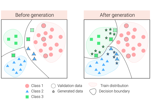
Figure 1. Long-tail distributions consist of few categories with many samples (head of the long tail, in red) and many categories with few to very-few samples (green, blue). Due to the larger diversity of the head classes, decision boundaries are often favourable for the head class, while being error-prone for the tail classes. The goal of our work is to generate meaningful additional features for the tail classes so that a balanced training set is created for the classifier. To this end, we estimate the distribution of the tail classes based on individualized instances and sample additional features through this calibrated tail distribution.

Modern machine learning is driven by large scale datasets, employed in both supervised (Russakovsky et al., 2015; Parkhi et al., 2015; Gemmeke et al., 2017) and self-supervised (Prakash et al., 2021; Miech et al., 2019; Sun et al., 2017; Sharma et al., 2018) scenarios. However, creation of these labeled datasets is a challenging and costly affair (Acuna et al., 2021) and may also lead to unforeseen biases (Tsipras et al., 2020). Often, these datasets are created by querying images through a search engine (Russakovsky et al., 2015; Parkhi et al., 2015), followed by post-processing and “cleaning” to ensure a balanced distribution that has an (approximately) equal number of instances for each category.

However, the world we live in is naturally long-tail, and like the language modality, even visual data follows the Zipf’s law (Zipf, 1949; van Horn et al., 2018). This is easily illustrated through examples we encounter in our daily lives: people living in a city are more likely to see multiple instances and a large diversity of cars than elephants for transportation, and tables and chairs than tree stumps as furniture. This natural distribution of categories is reflected in the datasets that are collected through community efforts, e.g. iNaturalist (van Horn et al., 2018) that features a large image collection of biodiversity; or annotations for a collection of randomly sampled raw data – action labels from the Atomic Visual Actions dataset (Gu et al., 2018); or interaction and relationship labels from movie datasets (Vicol et al., 2018).

Modern deep learning methods perform well on balanced distributions and have even shown super-human performance for some datasets and tasks in diverse domains including image classification (He et al., 2015) and language understanding (Wang et al., 2019a). This has led to a steadily growing interest in adapting methods to work well with few training samples – few-shot learning (Cao et al., 2020; Wang et al., 2019c; Dhillon et al., 2020; Mangla et al., 2020; Wang et al., 2019b) or naturally occurring long-tail distributions (Kang et al., 2020; Lin et al., 2017; Zhou et al., 2020; Tang et al., 2020; Iscen et al., 2021). Interestingly, it is observed that popular techniques used in shallow learning (e.g. SVMs) such as loss re-weighting or balanced sampling (Japkowicz, 2000) do not perform well when they are applied with deep neural networks, as they may hurt the representation learning (Kang et al., 2020; Zhou et al., 2020). Instead, decoupling the feature learning (i.e. CNN backbone) from the classifier (i.e. final linear layers) is found to be necessary and useful (Kang et al., 2020).

In this work, we are interested in answering the following question. Can we learn to generate feature representations for the impoverished tail classes, instead of requiring re-weighting (e.g. (Zhou et al., 2020)) or multi-network distillation (e.g. (Iscen et al., 2021)) strategies? Inspired by the recent success of distribution calibration on few-shot learning (Yang et al., 2021), we estimate and calibrate the feature distribution of tail classes to sample additional features that are in turn used to train a classifier - we term this as TailCalibration (see Fig. 1). Note that our work is different from (Chawla et al., 2002; Kim et al., 2020; Damien Dablain, 2021) that attempt to reconstruct or generate images for the tail class; or from (Zhang et al., 2017; Verma et al., 2019) that use convex combinations of input samples or features and their labels. TailCalibration is agnostic to the training approach of the backbone, and therefore, adopting better classification setups (e.g. CosineCE (Luo et al., 2018)) or using distillation (e.g. CBD (Iscen et al., 2021)) can further improve overall performance.

Our contribution can be summarized as follows: We explore feature generation as a means to address the challenges of long-tail classification, and show that TailCalibration, an adapted version of (Yang et al., 2021), is an effective strategy to generate meaningful additional features (Sec. 3). We empirically validate our approach through multiple ablation studies on the CIFAR-100-LT achieving the state-of-the-art performance (Sec. 4). Our analysis also holds for a long-tailed version of a similarly sized dataset called mini-ImageNet-LT (Vinyals et al., 2016) that had been introduced for few-shot learning. We also present a qualitative analysis of generated features using t-SNE visualizations and analyze the category-level nearest neighbors used to calibrate the tail class distributions.

2. Related Work

We discuss and contrast related work on long-tail classification with our proposed approach. While imbalanced learning has had a long history, we focus primarily on modern techniques applied to deep learning. In general, we can group related works in 4 broad categories: (i) modifications to the loss function or re-weighting of samples; (ii) decoupling the learning process of the representation and classifier; (iii) using distillation or multiple experts; and (iv) perhaps closest to our work, ideas related to sample or feature generation.

2.1. Re-weighting or Adapting the Loss Function

Class re-weighting or balanced sampling are popular approaches to deal with long-tail datasets especially in shallow architectures (Japkowicz, 2000). However, with deep learning, as the same loss function trains both the representation network and the classifier, the above ideas are not directly applicable.

The cross-entropy (CE) loss is modified to down-weight easier examples while focusing on harder ones (Lin et al., 2017), or to include the effective number of training samples via a re-weighting term (Cui et al., 2019). As an alternative to CE, there has also been work on deriving a class-specific margin parameter to be inversely proportional to the fourth root of number of samples for a margin-based loss (Cao et al., 2019). Long-tail classification and label corruption are also attempted simultaneously through meta-learning networks for re-weighting instances (Ren et al., 2018; Shu et al., 2019). Recently, a simple logit adjustment that can be applied post-hoc to trained models (Menon et al., 2021) is proposed as a means to unify many of the above approaches.

A few different perspectives applied to long-tail classification include viewing it as a domain adaptation task (target shift) (Jamal et al., 2020; Hong et al., 2021), or as a causal framework where stochastic gradient descent’s momentum term is treated as a confounder (Tang et al., 2020).

Our work does not belong to this category and can be thought of as orthogonal to any of the techniques above.

2.2. Decoupling Representation and Classifier

One of the key challenges of deep learning on long-tail datasets is exposed by (Kang et al., 2020; Zhou et al., 2020). Both works demonstrate that (i) representation learning suffers when applying balancing or re-weighting techniques on end-to-end training paradigms, and (ii) classifier performance of tail classes is adversely impacted when using standard instance sampling. As remedies, a two stage approach is suggested. In the first stage, usual end-to-end training is performed using instance sampling. In the second stage, the classifier is decoupled from the network and is trained with balanced sampling (Kang et al., 2020). While this two-stage strategy improves the performance, (Zhong et al., 2021) discovers that this may lead to domain shift between the representation and the classifier parts when seen from the perspective of transfer learning and proposes MiSLAS - a batch normalization based trick to resolve this. On similar lines, a dual network with shared backbone is proposed by (Zhou et al., 2020) with an adaptive trade-off parameter that balances the two objectives.

Our work is related to the above - we also decouple the training of the backbone from the classifier. The key difference is that instead of balanced sampling, we attempt to generate meaningful features for the tail classes that are subsequently used to train the classifier.

2.3. Distilling Information across Networks

An alternative approach to long-tail classification is using (multiple) teachers to distill information into a student network. One idea here involves learning separate classifiers for sets of categories such that the segregated imbalance factor is reduced before combining them (Xiang et al., 2020). Along those lines, RIDE (Wang et al., 2021) trains multiple experts with shared earlier layers and routes the inference through a subset of trained experts to improve tail class performance. These subset of experts can be self-distilled from the a larger subset of experts for further improvement. An alternative idea considers an ensemble of teachers trained on instance sampling that are used to uphold the quality of the representation network while training the student on a balanced sampling schedule (Iscen et al., 2021).

Our strategy is orthogonal to this approach and we show that applying TailCalibration on the distilled model from (Iscen et al., 2021) further improves performance.

2.4. Instance or Feature Generation

The final set of approaches address the challenges of long-tail classification through generation or augmentation of samples or features. Among sample generation, SMOTE (Chawla et al., 2002) is an old but popular choice that generates new instances through interpolation between samples of the same (often, the tail) class. Parallel to our work, SMOTE has been extended to deep learning where an encoder-decoder framework is used to generate additional images, DeepSMOTE (Damien Dablain, 2021). Similar to SMOTE, mixup is a general supervised learning paradigm that allows models to learn from convex combinations of not only input samples, but also their labels (Zhang et al., 2017). Specifically designed for visual long-tail classification, M2m translation transfers the diversity of samples from the head class to the tail through gradient updates, resulting in minor visual transformations that lead to significant impact on classification scores (Kim et al., 2020). Similar to M2m, (Chu et al., 2020) explicitly models class-specific and class-generic features which are then mixed together to transfer the sample diversity from the head class to the tail.

While mixup is applied on the input space, manifold mixup is applied on the semantic (feature) space (Verma et al., 2019) and is effective at generating convex feature combinations. Specific data augmentation strategies relevant for long-tail classification transfer the implicit knowledge of features from the head classes that exhibit a high variance, to the tail classes that lack intra-class diversity (Liu et al., 2020). This is done by constructing a feature cloud around the existing tail data points to match the head class variance. A recent work MODALS (Cheung and Yeung, 2021) suggests multiple modality agnostic feature augmentation strategies based on hard example interpolation, extrapolation, and Gaussian noise around the samples.

Our work is related to these ideas, but differs in the actual method for feature generation. By calibrating distributions we expect to learn from the diversity of head classes and generate features for tail classes to balance the inputs seen by the classifier.

3. Method

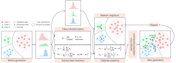
Figure 2. We visualize the process of feature generation. We first estimate the class statistics, and apply the Tukey transformation to convert the data into a distribution closer to a Gaussian. We find the nearest neighbor categories for each instance, calibrate the tail class distribution, and sample from this to generate additional features. The process is repeated until all categories have balanced number of features, which are used as training data for the classifier.

We present details of our proposed method, TailCalibration, that generates additional features for the tail classes. We start by formulating the long-tail classification task through some notation and a discussion of multiple strategies to train the backbone network.

3.1. Problem Definition

We address $K$ class supervised classification on a training dataset $\mathcal{D}=\{(\mathbf{x}_{i},c_{i})\}_{i=1}^{N}$ with $N$ samples. $\mathbf{x}_{i}$ represents the $i^{\mathrm{th}}$ image and $\mathbf{y}_{i}$ is the one-hot encoding of the category label $c_{i}\in\{1,\ldots,K\}$. For simplicity, we denote the set of samples belonging to category $k$ by $\mathcal{D}_{k}$, and denote its cardinality by $N_{k}=|\mathcal{D}_{k}|$. A long-tail setup can be defined by ordering the number of samples per category, i.e. $N_{1}\geq N_{2}\geq\ldots\geq N_{K}$ (without loss of generality), such that $\sum_{k}N_{k}=N$. The imbalance factor of the dataset is indicated as the ratio of samples in the head to tail class, $N_{1}/N_{K}$, where a higher imbalance often translates to worse performance on the tail categories.

We train a network $\Phi$ consisting of two components: (i) a backbone or representation network (CNN for images) that translates an image to a feature representation $f(\mathbf{x}_{i})=\mathbf{z}_{i}$ where $\mathbf{z}_{i}\in\mathbb{R}^{D}$, and (ii) a classifier $\mathbf{W}\in\mathbb{R}^{K\times D}$ that predicts the category specific scores (logits) $g(\mathbf{z}_{i})=\mathbf{s}_{i}$. When not specified otherwise, we assume $\mathbf{s}_{i}=g(\mathbf{z}_{i})=\mathbf{W}\mathbf{z}_{i}$. We ignore writing the bias term of the linear layer for brevity.

3.2. Training the Backbone

Our approach on generating features is independent from the manner in which the representation network is trained. Below, we present three ways of obtaining a trained backbone network $f$.

CE

We consider a batch-wise training approach with instance sampling, where each sample $\mathbf{x}_{i}$ has equal probability of being considered as part of a mini-batch $\mathcal{B}$. Specifically, the parameters of the backbone $f$ and the classifier $g$ are trained end-to-end using the cross-entropy (CE) loss:

(1) $$L_{CE}=-\sum_{i}\mathbf{y}_{i}\log(\mathbf{p}_{i})\,,$$

where $\mathbf{p}_{i}$ is a vector of probabilities obtained by transforming the logits $\mathbf{s}_{i}$ through the softmax operation.

CosineCE

As an alternative to the standard dot-product classifier, a cosine normalization based classifier is proposed to reduce the variance of the output neuron (Luo et al., 2018). The key difference lies in the computation of the dot product – the feature vector $\mathbf{z}_{i}$ and each row (category $k$) of the classifier, $\mathbf{w}_{k}$, are $\ell_{2}$-normalized prior to computing the dot product. The logit score for sample $\mathbf{x}_{i}$ and category $k$ is computed as follows:

(2) $$s^{\mathrm{CosCE}}_{ik}=\gamma\frac{\mathbf{z}_{i}^{\top}\mathbf{w}_{k}}{\|\mathbf{z}_{i}\|_{2}\|\mathbf{w}_{k}\|_{2}}\,~{}~{}~{}~{}~{}~{}~{}~{}~{}~{}~{}\text{ where }\mathbf{z}_{i}=f(\mathbf{x}_{i}),$$

where $\gamma\in\mathbb{R}_{+}$ is a positive normalization constant that ensures that $s^{\mathrm{CosCE}}_{ik}\in[-\gamma,\gamma]$. We treat $\gamma$ as a learnable parameter and use the softplus operator to ensure that it remains positive. We recall that the operator is defined as $\forall x\in\mathbb{R}$, softplus$(x)=\log(1+e^{x})$. The loss function used to train the model remains unchanged from the above Eq. (1).

This formulation has also been adopted by recent works on few-shot learning (Gidaris and Komodakis, 2018) and long-tail classification (Iscen et al., 2021). In particular, the cosine similarity based score computation embeds all samples close to a single point on the hypersphere (i.e. a $(D-1)$-sphere embedded in $\mathbb{R}^{D}$) indicated by the classifier vector. We believe that this makes the distribution of features on the hypersphere closely resemble a Gaussian distribution or a von Mises-Fisher distribution (Banerjee et al., 2005). We will show the benefits of using CosineCE through our ablation studies.

Class-balanced Distillation (CBD)

Parallel to our work, Iscen et al. (Iscen et al., 2021) show the use of teacher-student distillation with the goal of improving both the backbone representation and the classifier. We briefly summarize their approach. First, a teacher network $\Phi_{T}:(f_{T},g_{T})$ is trained using standard instance sampling and the CosineCE classifier described above. Then, a student network $\Phi_{S}:(f_{S},g_{S})$ is trained with balanced sampling along with distillation, i.e. the intermediate feature representation $f_{S}(\mathbf{x}_{i})$ is constrained to be similar to $f_{T}(\mathbf{x}_{i})$, while harnessing the benefits of balanced sampling for the classifier $g_{S}$. We decouple the backbone network trained through a combination of the classification and distillation losses, and show that TailCalibration can use these improvements to obtain additional performance gains.

3.3. TailCalibration

The primary objective of our work is to generate additional features $\mathbf{z}^{*}$ such that they can be used to balance the data that is used to train the classifier. Distribution calibration (DC) was proposed recently in the context of few-shot learning: samples are generated for the few-shot classes by relying on statistics of the base classes (Yang et al., 2021). We investigate the applicability of DC in the context of long-tail classification, and present the generation process below.

Our approach can be simplified into three steps, also illustrated in Fig. 2. (i) We first estimate the distribution of each category based on a Gaussian assumption; (ii) Categorical neighbors of each instance in the tail classes are used to create a calibrated distribution; and (iii) We sample several new features from these distributions to balance the training data seen by a classifier.

All operations below are in the feature space. Given a trained backbone (discussed in Sec. 3.2), we first precompute feature representations for the entire dataset. These features of true samples are denoted by $\mathcal{F}=\{\mathbf{z}_{i}\}_{i=1}^{N}$. $\mathcal{F}_{k}$ denotes features of images corresponding to the subset $\mathcal{D}_{k}$, or belonging to the category $k$.

Due to the inherent randomness in sampling from a distribution, we can generate features multiple times and use them as a fresh dataset from which the classifier can learn something new in each epoch.

Class statistics

We start by computing the statistics for each category, assuming that the feature distribution is Gaussian. Note that this assumption may be particularly reasonable when using a backbone trained with the CosineCE loss function.

(3) $$\mu_{k} = \frac{1}{N_{k}}\sum_{i\in\mathcal{F}_{k}}\mathbf{z}_{i}\,,\mathrm{and}$$

(4) $$\Sigma_{k} = \frac{1}{N_{k}-1}\sum_{i\in\mathcal{F}_{k}}(\mathbf{z}_{i}-\mu_{k})(\mathbf{z}_{i}-\mu_{k})^{T}\,,$$

where $\mu_{k}\in\mathbb{R}^{D}$ and $\Sigma_{k}\in\mathbb{R}^{D\times D}$ denote the mean and full covariance of the Gaussian distribution for category $k$.

Tukey’s Ladder of Powers transformation

Sometimes referred to as the Bulging rule, this transformation helps change the shape of a skewed distribution so that it becomes closer to a Normal distribution (Tukey, 1977). In particular, it is applied to each dimension of the feature as follows:

(5) $$\tilde{\mathbf{z}}_{i}=\begin{cases}\mathbf{z}_{i}^{\lambda}&\text{if $\lambda\neq 0$}\\ \log(\mathbf{z}_{i})&\text{otherwise}\,.\end{cases}$$

where $\lambda>0$ is a hyperparameter of our model and $\mathbf{z}_{i}^{\lambda}$ raises each element of $\mathbf{z}_{i}$ to the power $\lambda$. In fact, $\lambda\simeq 1$ is found to perform well for most of our experiments.

Calibration and generation

For each class, we sample $N_{1}-N_{k}$ additional features, such that the resulting feature dataset is completely balanced and all classes have $N_{1}$ instances. Sampling is performed based on an instance specific calibrated distribution. Specifically, each $\mathbf{z}_{ik}$ ($i^{\mathrm{th}}$ feature from category $k$) is responsible for generating $\left[N_{1}/N_{k}-1\right]_{+}$ features where $[x]_{+}$ rounds $x$ to the nearest integer greater than or equal to $x$. As $N_{1}/N_{k}$ may be a fraction, we randomly choose an appropriate number of $\mathbf{z}_{ik}$ so as to obtain a total of $N_{1}$ samples.

Next, we compute the distances between class means and the selected feature. For each feature $\mathbf{z}_{i}$, we first compute the distance between the instance and category means as

(6) $$\forall k,\,d_{ik}=\|\tilde{\mathbf{z}}_{i}-\mu_{k}\|_{2}.$$

We identify the set of $M$ category indices that are neighbors $\mathcal{N}_{i}$ with smallest distance $d_{ik}$. Note that the distance computation uses the Tukey transformed feature $\tilde{\mathbf{z}}_{i}$.

The calibrated distribution is obtained as

(7) $$\mu_{\mathbf{z}_{i}} = \frac{1}{M+1}\left(\sum_{k\in\mathcal{N}_{i}}\mu_{k}+\tilde{\mathbf{z}}_{i}\right)$$

(8) $$\Sigma_{\mathbf{z}_{i}} = \frac{1}{M}\left(\sum_{k\in\mathcal{N}_{i}}\Sigma_{k}\right)+\alpha\,,$$

where $\alpha$ is an optional constant hyper-parameter to increase the spread of the calibrated distribution. We found that $\alpha=0$ works reasonably well for multiple experiments.

Sampling

We initialize a multi-variate Gaussian distribution for each instance $\mathbf{z}_{i}$, and generate new features with the same associated class label as $c_{i}$. We denote the generated features for category $k$ as $\mathcal{F}_{k}^{*}$, and together, $|\mathcal{F}_{k}\cup\mathcal{F}_{k}^{*}|=N_{1}$. This combined set of features is generated for all categories and used to train the classifier $g$.

$\ell_{2}$-normalized calibration

For the CosineCE backbone, we $\ell_{2}$-normalize the features $\mathbf{z}_{i}$ before feeding them to the TailCalibration pipeline, both for gathering statistics and Tukey transformation.

4. Experiments

In this section, we start by presenting a brief overview of the dataset and implementation details for our methods. We present some ablation studies comparing different aspects of the model, and finally perform a thorough comparison of our work against state-of-the-art approaches. We also include some analysis to obtain a better understanding of the feature generation process.

4.1. Datasets and Experimental Setup

We benchmark our proposed method across two datasets, CIFAR-100-LT and mini-ImageNet-LT.

CIFAR-100-LT

CIFAR-100 is a balanced dataset containing 60K images from 100 categories, with 50K in train and 10K in validation. We use the synthetically created long-tail variants that have also been used by previous works (Cao et al., 2019; Zhou et al., 2020). There are three versions of the CIFAR-100-LT dataset, with the imbalance factor ($N_{1}/N_{K}$) of $\{10,50,100\}$. An exponential decay is used for determining $N_{k}$ in between. Note that a higher imbalance factor mimics a stronger long-tail problem and is typically more challenging - we will see this through the performance of baseline models.

As the synthetically created variants involve randomly selecting images, all experiments are replicated with 3 seeds where different sets of images are selected. The average performance over all seeds is reported when not mentioned otherwise. As we will see in the ablation studies, this random sub-sampling often leads to a high variance, but we observe consistent improvements by using our approach. For evaluation, we use the entire balanced validation set of 10K images, 100 samples for each of the 100 categories.

mini-ImageNet-LT

mini-ImageNet was proposed by (Vinyals et al., 2016) for few-shot learning evaluation, in an attempt to have a dataset like ImageNet while requiring fewer resources. Similar to the statistics for CIFAR-100-LT with an imbalance factor of 100, we construct a long-tailed variant of mini-ImageNet that features all the 100 classes and an imbalanced training set with $N_{1}=500$ and $N_{K}=5$ images. For evaluation, both the validation and test sets are balanced and contain 10K images, 100 samples for each of the 100 categories.

We report performance as accuracy. Note that average per-sample accuracy is equivalent to average per-class accuracy due to the balanced evaluation sets in both datasets.

4.2. Implementation details

Implementation details for CIFAR100-LT

We follow a similar setup to (Zhou et al., 2020): the backbone is a ResNet-32 (He et al., 2016) trained by mini-batch stochastic gradient descent (SGD) with a momentum of 0.9 and a batch size of 128. For a fair comparison, we tune the other parameters to match the baseline accuracy of the rest of the reported works. The learning rate is decayed by a cosine scheduler (Loshchilov and Hutter, 2017) from 0.2 to 0.0 in 150 epochs, and a weight decay of $5\times 10^{-5}$ is used. We train our models on a single NVIDIA 1080Ti GPU.

Implementation details for mini-ImageNet-LT

We follow a similar setup to (Tang et al., 2020; Kang et al., 2020): the backbone is a ResNeXt-50 trained by minibatch stochastic gradient descent (SGD) with a momentum of 0.9 for 111 epochs on a batch size of 512. Through hyperparameter tuning, we found that weight decay of $5\times 10^{-4}$ with a constant learning rate of 0.01 provides a better performing baseline. We train all the models on a NVIDIA Tesla P100 GPU.

For the TailCalibration feature generation, we use the hyperparameters as stated in Table 1. Subsequently, the classifier is re-trained with a constant learning rate of 0.001 for CIFAR-100-LT and 0.01 for mini-ImageNet-LT. While the weight decay for retraining the classifier remains the same as the backbone for CIFAR-100-LT, we found that decreasing the weight decay from $5\times 10^{-4}$ to $5\times 10^{-5}$ improves performance for mini-ImageNet-LT.

Table 1. Hyperparameters used in TailCalibration feature generation across various imbalance ratios and datasets.

Hyperparameters	CIFAR-100-LT			mini-
	Imbalance Ratios			-ImageNet-
	100	50	10	-LT
$\lambda$ (Tukey value)	1.0	0.9	0.9	1.0
$M$ (Number of categories)	3	2	2	2
$\alpha$ (Spread of generated features)	0.0	0.2	0.0	0.1

4.3. Ablation studies on CIFAR-100-LT

We present a few ablation studies to compare various aspects of our proposed method. Note that we do all the necessary ablations only with CIFAR-100-LT and use the findings to guide our decisions on mini-ImageNet-LT.

$\ell_{2}$-normalization

Table 2. Ablation study comparing the impact of $\ell_{2}$-normalization of features prior to TailCalibration. Backbone: CosineCE, Feature generation: TailCalib.

Method	Imbalance Ratios
	100	50	10
without $\ell_{2}$-normalization	42.62	49.17	58.12
with $\ell_{2}$-normalization	43.03	49.18	58.60

As indicated in the last paragraph of Sec. 3.3, when using CosineCE, we observed that it is better to $\ell_{2}$-normalize the feature vectors $\mathbf{z}_{i}$ before and after the generation. We show the impact of this normalization in Table 2. Imbalance factors 100 and 10 see a small but consistent improvement across all three seeds, pointing to the relevance of this modification: +0.21%, +0.64%, and +0.38% for imbalance 100 and +0.77%, +0.4%, and +0.29% for imbalance 10. For imbalance 50, we see a small improvement for 2 of 3 seeds: +0.12%, +0.09%, and -0.19%, resulting in an overall negligible performance difference.

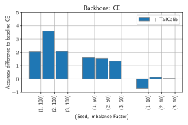
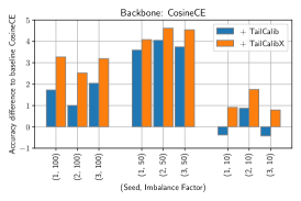
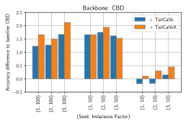
Figure 3. Performance improvement in absolute percentage points across TailCalib and TailCalibX for all three backbones: CE (left), CosineCE (middle), CBD (right). On the x-axis, we indicate the seed and imbalance factor of each run. Please refer to Table 3 for averaged performance scores across the 3 seeds.

Backbones

Table 3. Ablation study comparing the impact of backbones: CE vs. CosineCE vs. CBD. We also see that generating features multiple times can be beneficial for training: TailCalib vs. TailCalibX.

Backbone	Feature	Imbalance Ratios
	Generation	100	50	10
CE	-	39.89	44.88	57.00
	TailCalib	42.28	46.37	56.81
CosineCE	-	41.44	45.72	58.58
	TailCalib	43.03	49.18	58.60
	TailCalibX	44.44	49.80	59.73
CBD (Iscen et al., 2021)	-	44.83	49.19	60.85
	TailCalib	46.22	50.87	60.78
	TailCalibX	46.59	50.90	61.13

We presented three main strategies to train our backbone in Sec. 3.2. Table 3 reports performance when applying TailCalibration (abbreviated as TailCalib) for features precomputed from various backbones (averaged across 3 seeds). Firstly, note that CosineCE outperforms CE, while CBD with teacher-student distillation outperforms both. TailCalibration shows a consistent improvement over backbones, especially for the higher imbalance factors of 50 and 100.

Training with multiple rounds of generation

As the feature generation process is quite fast, we can afford to generate samples on-the-fly for each epoch during the training of the classifier. In particular, we propose TailCalibX, denoting that TailCalib is employed multiple times. Specifically, we generate a set of features once every epoch and use them to train the classifier. We show the results for this experiment in Table 3. TailCalibX provides incremental performance boosts over TailCalib.

Trends across different seeds

The variation across seeds is typically high as changing the seed not only changes the random initialization of the base network (this has a small impact), but also leads to the selection of a different subset of CIFAR-100 images for creating the synthetically imbalanced training data (this has a large impact). This is especially true for imbalance factor 50 and 10; we suspect that as there are very few training samples in the tail categories for imbalance factor 100, which samples are selected does not matter as much. For example, the accuracy of the CE baseline across 3 seeds is (43.8%, 44.8%, 46.1%) for imbalance factor 50.

Fig. 3 shows the absolute percentage points performance improvement over the specific backbone for each seed. We observe consistent performance improvement over progressively harder backbones by applying TailCalib or TailCalibX across various seeds.

We can also see that while TailCalib may fail to provide performance improvements for low imbalance factors (CosineCE and CBD, imbalance 10), TailCalibX always provides a small boost. This indicates that the feature generation process may not be very reliable for datasets with a small long-tail effect, but the classifier can still extract meaningful information from multiple rounds of generation.

4.4. Comparison to state-of-the-art

We compare our proposed approach against several previous works grouping them in a manner similar to our related work in Sec. 2.

Table 4. Comparison of our approach (TailCalib, TailCalibX) against previous works on CIFAR-100-LT. Methods with a * indicate results produced by our re-implementations, please see the text for details about the implementation. Best results are highlighted in bold, next best and notable results with underline.

Type	Method	Imbalance Ratios
		100	50	10
Baseline	*CE	39.89	44.88	57.00
	*CosineCE	41.44	45.72	58.58
	Focal Loss (Lin et al., 2017)	38.41	44.32	55.78
	Class-Balanced Focal (Cui et al., 2019)	39.60	45.32	57.99
	L2RW (Ren et al., 2018)	38.90	46.83	52.12
Loss or	Meta-Weight Net (Shu et al., 2019)	41.61	45.66	58.91
Re-weighting	Domain Adaptation (Jamal et al., 2020)	39.31	48.53	59.58
	LDAM-DRW (Cao et al., 2019)	42.04	-	58.71
	Logit adjustment (Menon et al., 2021)	43.89	-	-
	GBM (Tang et al., 2020)	44.1	50.3	59.6
Decouple	*cRT (Kang et al., 2020)	42.63	47.26	57.61
	BBN (Zhou et al., 2020)	42.56	47.02	59.12
Distillation	LFME (Xiang et al., 2020)	42.3	-	-
	*CBD (Iscen et al., 2021)	44.83	49.19	60.85
Generation	M2M (Kim et al., 2020)	42.9	-	58.2
	mixup (Zhang et al., 2017)	39.54	44.99	58.02
	Manifold mixup (Verma et al., 2019)	38.25	43.09	56.55
	*MODALS (Cheung and Yeung, 2021)	42.813	47.57	58.53
*Ours	CosineCE + TailCalib	43.03	49.18	58.60
	CosineCE + TailCalibX	44.44	49.80	59.73
	CBD + TailCalibX	46.59	50.90	61.13

Table 5. Comparison of our approach (TailCalib, TailCalibX) against previous works on mini-ImageNet-LT. Since we introduce using mini-ImageNet in a long-tail variant, all methods are our re-implementations. Best results are highlighted in bold, next best and notable results with underline.

Type	Method	Many	Mid	Few	All
Baseline	CE	57.77	29.42	8.06	32.94
	CosineCE	65.45	29.37	8.6	35.77
Decouple	cRT (Kang et al., 2020)	66.00	31.99	29.3	43.09
Distillation	CBD (Iscen et al., 2021)	67.34	35.00	23.06	42.74
Generation	MODALS (Cheung and Yeung, 2021)	66.62	28.65	11.06	36.67
	mixup (Zhang et al., 2017)	64.71	27.51	8.1	34.72
Ours	CosineCE + TailCalib	68.05	32.59	25.13	42.77
	CosineCE + TailCalibX	68.3	34.3	29.4	44.73

Results for most methods are taken from the respective papers or BBN (Zhou et al., 2020). For the methods that did not report results on CIFAR-100-LT or mini-ImageNet-LT, we present additional details of our re-implementation.

• For CE and CosineCE, we choose hyperparameters (learning rate scheduler, number of epochs, etc.) to match the performance of CE on a previously reported work, BBN (Zhou et al., 2020).

• cRT (Kang et al., 2020) does not provide results on the CIFAR-100-LT and mini-ImageNet-LT datasets. We use their publicly available code to generate results for both the datasets.

• CBD is a recent, and to the best of our knowledge, unpublished work (Iscen et al., 2021). Through email conversations with the authors, we verified our implementation and present results with a single teacher trained on the both datasets.

• MODALS (Cheung and Yeung, 2021) was trained with the Gaussian noise augmentation. We choose $\lambda=0.01$ after performing a sweep across $[0.1,0.01,0.001]$.

• For mixup (Zhang et al., 2017), we choose $\alpha=0.01$ after performing a sweep across $[0.01,0.1,0.2,0.3,0.5,0.7]$.

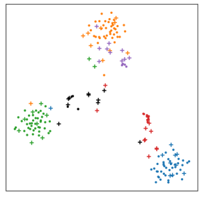
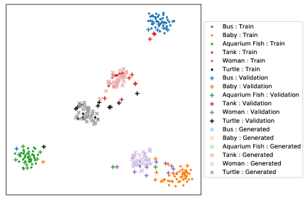
Figure 4. t-SNE visualization of a few head and tail classes from CIFAR-100-LT. The plot on the left is before generation, and the plot on the right is after generation. We show 10 validation samples for each class and limit to 40 training + generated samples for ease of interpretation. Markers: $\bf\cdot$ (dot) indicate training samples; $+$ (plus) are validation samples; and $\times$ (cross) are generated features also shown with a lighter version of the base color (e.g. black-gray for turtle). Head categories: bus (273), baby (455), aquarium fish (477). Tail categories: tank (9), woman (5), turtle (6). Class size is indicated in parenthesis. Please refer to the text, Sec. 4.5 for a more thorough discussion. Best seen in colour.

CIFAR-100-LT (Table 4)

Firstly, note that the CosineCE training paradigm is superior to CE, and in fact, outperforms several loss re-weighting based methods. CosineCE + TailCalibX outperforms all previous works ignoring distillation. In fact, it achieves performance close to CBD (Iscen et al., 2021) (especially on imbalance factors 100 and 50) that trains two networks - a teacher and student, and benefits from the advantages of ensembling. Finally, applying TailCalibX on top of a trained CBD model results in further performance improvements of 1-2% notably for imbalance factors 100 and 50.

mini-ImageNet-LT (Table 5)

TailCalibX outperforms all previous works. As compared to the CosineCE baseline, not only does it improve the accuracy for tail classes (few) by over 20%, we also see performance improvements for both the middle classes (mid, +4.93%) and head classes (many, +2.85%) as well. Surprisingly, CBD performs worse than classifier re-training (cRT), hence, we omit evaluation of TailCalibration as applied to a backbone trained with CBD.

4.5. Analysis

tSNE visualization

Fig. 4 shows a few feature embeddings computed using t-SNE (van der Maaten and Hinton, 2008) for head and tail categories from the CIFAR-100-LT dataset. For visual clarity, we show 10 validation samples for each class and up to 40 training + generated samples. We randomly choose 3 pairs of visually similar categories: tank and bus, woman and baby, and aquarium fish and turtle, such that one of them is from the bottom 15 tail categories, while the second belongs to the top 15 head categories.

In the left plot, before feature generation, we see that the validation samples ($+$) from the tail categories are often confused with visually similar and larger head classes: (i) five samples of the tank (red) are located close to the bus (blue) cluster; and (ii) roughly 7 of 10 samples of the woman category (purple) are potentially confused as belonging to the baby class (orange). In the right plot, we generate features using TailCalibration and re-compute the t-SNE embeddings. We observe a noticeable reduction in errors, even on this randomly picked toy sample. Now, 3 of 5 tank samples are close to the bus cluster, and 4 of 7 woman samples are close to the baby cluster, while the others are more easily separable.

Class nearest neighbors

Table 6. Two most frequently chosen nearest neighbor categories to calibrate the distributions for generating features for 20 tail categories of CIFAR-100-LT dataset.

Tail category	# Train samples	Nearest neighbors
tank	9	tractor, pickup_truck
telephone	9	streetcar, keyboard
television	8	couch, lamp
tiger	8	leopard, lion
tractor	7	lawn_mower, train
train	7	tractor, road
trout	7	dinosaur, caterpillar
tulip	6	rabbit, cattle
turtle	6	telephone, ray
wardrobe	6	television, skyscraper
whale	6	otter, seal
willow_tree	5	rabbit, oak_tree
wolf	5	rabbit, possum
woman	5	man, girl
worm	5	ray, woman

Recall, to generate the calibrated tail distributions, we pick $M$ categories as nearest neighbors for each feature $\mathbf{z}_{ik}$. We analyze the classes that are most commonly used as nearest neighbors for the bottom 15 tail classes of the CIFAR-100-LT dataset in Table 6. The table shows the nearest neighbors for imbalance factor 100 and $M=3$. We observe that the class for which we wish to generate samples is often the nearest centroid and is ignored in the table for brevity.

This split of CIFAR-100-LT is sorted alphabetically, i.e. the classes with letter a belong to the head, and classes with letters towards the end of the alphabet form the tail. We see that nearest neighbors need not belong to the head classes, even though it may be common. For example, we see that tiger distribution draws from the lion class, or television from couch, possibly due to the fact that images with a television have additional furniture in them.

5. Conclusion and Future work

Learning to cope with long-tail distributions is an important problem for machine learning. Inspired by a recent work on few-shot learning (Yang et al., 2021), we explored one facet of this challenging task: feature generation as a means to balance the training data seen by a classifier. We analyzed the efficacy of distribution calibration and empirically validated that it can lead to substantial performance improvements. In this process, we achieved a new state-of-the-art on two synthetic datasets: CIFAR-100-LT and mini-ImageNet-LT, especially demonstrating that TailCalibration is orthogonal to, and can be combined with, other works such as CBD (Iscen et al., 2021), to yield additional improvements.

Future work

In the future, we wish to analyze the feature generation process in a more thorough manner. In particular, we hope to discover the underlying class-specific manifolds on which the features would be expected to lie. While our initial attempts at evaluating TailCalibration on ImageNet did not yield significant improvement, we would like to extend our evaluation to other long-tail datasets, both synthetic: ImageNet-LT (Liu et al., 2019) and Places-LT (Liu et al., 2019), and natural: iNaturalist (van Horn et al., 2018) or FineFoods dataset (Min et al., 2021). Another possibility is to exploit the hierarchy of categories and learn appropriate models such as hyperbolic representations (Law et al., 2019) or their generalization to pseudo-Riemannian manifolds of constant nonzero curvature (Law and Stam, 2020).

Acknowledgments

This work has been partly supported by the funding received from DST through the IMPRINT program (IMP / 2019 / 000250).

References

- (1)
- Acuna et al. (2021) David Acuna, Guojun Zhang, Marc T. Law, and Sanja Fidler. 2021. f-Domain Adversarial Learning: Theory and Algorithms. In International Conference on Machine Learning (ICML).
- Banerjee et al. (2005) Arindam Banerjee, Inderjit S Dhillon, Joydeep Ghosh, Suvrit Sra, and Greg Ridgeway. 2005. Clustering on the Unit Hypersphere using von Mises-Fisher Distributions. Journal of Machine Learning Research 6, 9 (2005).
- Cao et al. (2019) Kaidi Cao, Colin Wei, Adrien Gaidon, Nikos Arechiga, and Tengyu Ma. 2019. Learning Imbalanced Datasets with Label-Distribution-Aware Margin Loss. In Advances in Neural Information Processing Systems (NeurIPS).
- Cao et al. (2020) Tianshi Cao, Marc T Law, and Sanja Fidler. 2020. A Theoretical Analysis of the Number of Shots in Few-Shot Learning. In International Conference on Learning Representations (ICLR).
- Chawla et al. (2002) Nitesh V. Chawla, Kevin W. Bowyer, Lawrence O. Hall, and W. Philip Kegelmeyer. 2002. SMOTE: Synthetic Minority Over-sampling Technique. Journal of Artificial Intelligence Research (JAIR) 16 (2002), 321–357.
- Cheung and Yeung (2021) Tsz-Him Cheung and Dit-Yan Yeung. 2021. MODALS: Modality-agnostic Automated Data Augmentation in the Latent Space. In International Conference on Learning Representations (ICLR).
- Chu et al. (2020) Peng Chu, Xiao Bian, Shaopeng Liu, and Haibin Ling. 2020. Feature space augmentation for long-tailed data. In European Conference on Computer Vision (ECCV).
- Cui et al. (2019) Yin Cui, Menglin Jia, Tsung-Yi Lin, Yang Song, and Serge Belongie. 2019. Class-balanced loss based on effective number of samples. In Conference on Computer Vision and Pattern Recognition (CVPR).
- Damien Dablain (2021) Nitesh V. Chawla Damien Dablain, Bartosz Krawczyk. 2021. DeepSMOTE: Fusing Deep Learning and SMOTE for Imbalanced Data. In arXiv:2105.02340.
- Dhillon et al. (2020) Guneet Singh Dhillon, Pratik Chaudhari, Avinash Ravichandran, and Stefano Soatto. 2020. A Baseline for Few-Shot Image Classification. In International Conference on Learning Representations (ICLR).
- Gemmeke et al. (2017) Jort F. Gemmeke, Daniel P. W. Ellis, Dylan Freedman, Aren Jansen, Wade Lawrence, R. Channing Moore, Manoj Plakal, and Marvin Ritter. 2017. Audio Set: An ontology and human-labeled dataset for audio events. In International Conference on Audio, Speech, and Signal Processing (ICASSP).
- Gidaris and Komodakis (2018) Spyros Gidaris and Nikos Komodakis. 2018. Dynamic Few-shot Visual Learning without Forgetting. In Conference on Computer Vision and Pattern Recognition (CVPR).
- Gu et al. (2018) Chunhui Gu, Chen Sun, David A. Ross, Carl Vondrick, Caroline Pantofaru, Yeqing Li, Sudheendra Vijayanarasimhan, George Toderici, Susanna Ricco, Rahul Sukthankar, Cordelia Schmid, and Jitendra Malik. 2018. AVA: A Video Dataset of Spatio-temporally Localized Atomic Visual Actions. In Conference on Computer Vision and Pattern Recognition (CVPR).
- He et al. (2015) Kaiming He, Xiangyu Zhang, Shaoqing Ren, and Jian Sun. 2015. Delving Deep into Rectifiers: Surpassing Human-Level Performance on ImageNet Classification. In International Conference on Computer Vision (ICCV).
- He et al. (2016) Kaiming He, Xiangyu Zhang, Shaoqing Ren, and Jian Sun. 2016. Deep Residual Learning for Image Recognition. In Conference on Computer Vision and Pattern Recognition (CVPR).
- Hong et al. (2021) Youngkyu Hong, Seungju Han, Kwanghee Choi, Seokjun Seo, Beomsu Kim, and Buru Chang. 2021. Disentangling Label Distribution for Long-tailed Visual Recognition. In CVPR.
- Iscen et al. (2021) Ahmet Iscen, André Araujo, Boqing Gong, and Cordelia Schmid. 2021. Class-Balanced Distillation for Long-Tailed Visual Recognition. In arXiv:2104.05279.
- Jamal et al. (2020) Muhammad Abdullah Jamal, Matthew Brown, Ming-Hsuan Yang, Liqiang Wang, and Boqing Gong. 2020. Rethinking Class-Balanced Methods for Long-Tailed Visual Recognition from a Domain Adaptation Perspective. In Conference on Computer Vision and Pattern Recognition (CVPR).
- Japkowicz (2000) Nathalie Japkowicz. 2000. The Class Imbalance Problem: Significance and Strategies. In International Conference on Artificial Intelligence (IC-AI).
- Kang et al. (2020) Bingyi Kang, Saining Xie, Marcus Rohrbach, Zhicheng Yan, Albert Gordo, Jiashi Feng, and Yannis Kalantidis. 2020. Decoupling representation and classifier for long-tailed recognition. In International Conference on Learning Representations (ICLR).
- Kim et al. (2020) Jaehyung Kim, Jongheon Jeong, and Jinwoo Shin. 2020. M2m: Imbalanced Classification via Major-to-minor Translation. In Conference on Computer Vision and Pattern Recognition (CVPR).
- Law et al. (2019) Marc Law, Renjie Liao, Jake Snell, and Richard Zemel. 2019. Lorentzian Distance Learning for Hyperbolic Representations. In International Conference on Machine Learning (ICML).
- Law and Stam (2020) Marc Law and Jos Stam. 2020. Ultrahyperbolic Representation Learning. In Advances in Neural Information Processing Systems (NeurIPS).
- Lin et al. (2017) Tsung-Yi Lin, Priya Goyal, Ross Girshick, Kaiming He, and Piotr Dollár. 2017. Focal loss for dense object detection. In International Conference on Computer Vision (ICCV).
- Liu et al. (2020) Jialun Liu, Yifan Sun, Chuchu Han, Zhaopeng Dou, and Wenhui Li. 2020. Deep Representation Learning on Long-tailed Data: A Learnable Embedding Augmentation Perspective. In Conference on Computer Vision and Pattern Recognition (CVPR).
- Liu et al. (2019) Ziwei Liu, Zhongqi Miao, Xiaohang Zhan, Jiayun Wang, Boqing Gong, and Stella X. Yu. 2019. Large-Scale Long-Tailed Recognition in an Open World. In Conference on Computer Vision and Pattern Recognition (CVPR).
- Loshchilov and Hutter (2017) Ilya Loshchilov and Frank Hutter. 2017. SGDR: Stochastic gradient descent with warm restarts. In International Conference on Learning Representations (ICLR).
- Luo et al. (2018) Chunjie Luo, Jianfeng Zhan, Xiaohe Xue, Lei Wang, Rui Ren, and Qiang Yang. 2018. Cosine normalization: Using cosine similarity instead of dot product in neural networks. In International Conference on Artificial Neural Networks (ICANN).
- Mangla et al. (2020) Puneet Mangla, Mayank Singh, Abhishek Sinha, Nupur Kumari, Balaji K, and V N Balasubramanian. 2020. Charting the Right Manifold: Manifold Mixup for Few-shot Learning. In Winter Conference on Applications of Computer Vision (WACV).
- Menon et al. (2021) Aditya Krishna Menon, Sadeep Jayasumana, Ankit Singh Rawat, Himanshu Jain, Andreas Veit, and Sanjiv Kumar. 2021. Long-tail Learning via Logit Adjustment. In International Conference on Learning Representations (ICLR).
- Miech et al. (2019) Antoine Miech, Dimitri Zhukov, Jean-Baptiste Alayrac, Makarand Tapaswi, Ivan Laptev, and Josef Sivic. 2019. HowTo100M: Learning a Text-Video Embedding by Watching Hundred Million Narrated Video Clips. In International Conference on Computer Vision (ICCV).
- Min et al. (2021) Weiqing Min, Zhiling Wang, Yuxin Liu, Mengjiang Luo, Liping Kang, Xiaoming Wei, Xiaolin Wei, and Shuqiang Jiang. 2021. Large Scale Visual Food Recognition. arXiv:2103.16107 (2021).
- Parkhi et al. (2015) Omkar M. Parkhi, Andrea Vedaldi, and Andrew Zisserman. 2015. Deep Face Recognition. In British Machine Vision Conference (BMVC).
- Prakash et al. (2021) Aayush Prakash, Shoubhik Debnath, Jean-Francois Lafleche, Eric Cameracci, Gavriel State, Stan Birchfield, and Marc T. Law. 2021. Self-Supervised Real-to-Sim Scene Generation. In International Conference on Computer Vision (ICCV).
- Ren et al. (2018) Mengye Ren, Wenyuan Zeng, Bin Yang, and Raquel Urtasun. 2018. Learning to Reweight Examples for Robust Deep Learning. In International Conference on Machine Learning (ICML).
- Russakovsky et al. (2015) Olga Russakovsky, Jia Deng, Hao Su, Jonathan Krause, Sanjeev Satheesh, Sean Ma, Zhiheng Huang, Andrej Karpathy, Aditya Khosla, Michael Bernstein, Alexander C. Berg, and Li Fei-Fei. 2015. ImageNet Large Scale Visual Recognition Challenge. International Journal of Computer Vision (IJCV) 115 (2015), 211–252.
- Sharma et al. (2018) Piyush Sharma, Nan Ding, Sebastian Goodman, and Radu Soricut. 2018. Conceptual Captions: A Cleaned, Hypernymed, Image Alt-text Dataset for Automatic Image Captioning. In Proceedings of ACL.
- Shu et al. (2019) Jun Shu, Qi Xie, Lixuan Yi, Qian Zhao, Sanping Zhou, Zongben Xu, and Deyu Meng. 2019. Meta-weight-net: Learning an explicit mapping for sample weighting. In Advances in Neural Information Processing Systems (NeurIPS).
- Sun et al. (2017) Chen Sun, Abhinav Shrivastava, Saurabh Singh, and Abhinav Gupta. 2017. Revisiting Unreasonable Effectiveness of Data in Deep Learning Era. In International Conference on Computer Vision (ICCV).
- Tang et al. (2020) Kaihua Tang, Jianqiang Huang, and Hanwang Zhang. 2020. Long-Tailed Classification by Keeping the Good and Removing the Bad Momentum Causal Effect. In Advances in Neural Information Processing Systems (NeurIPS).
- Tsipras et al. (2020) Dimitris Tsipras, Shibani Santurkar, Logan Engstrom, Andrew Ilyas, and Aleksander Madry. 2020. From ImageNet to Image Classification: Contextualizing Progress on Benchmarks. In International Conference on Machine Learning (ICML).
- Tukey (1977) John W Tukey. 1977. Exploratory Data Analysis. Addison-Wesley.
- van der Maaten and Hinton (2008) Laurens van der Maaten and Geoffrey E. Hinton. 2008. Visualizing Data Using t-SNE. Journal of Machine Learning Recognition (JMLR) 9 (2008), 2579–2605.
- van Horn et al. (2018) Grant van Horn, Oisin Mac Aodha, Yang Song, Yin Cui, Chen Sun, Alex Shepard, Hartwig Adam, Pietro Perona, and Serge Belongie. 2018. The iNaturalist Species Classification and Detection Dataset. In Conference on Computer Vision and Pattern Recognition (CVPR).
- Verma et al. (2019) Vikas Verma, Alex Lamb, Christopher Beckham, Amir Najafi, Ioannis Mitliagkas, Aaron Courville, David Lopez-Paz, and Yoshua Bengio. 2019. Manifold Mixup: Better Representations by Interpolating Hidden States. In International Conference on Machine Learning (ICML).
- Vicol et al. (2018) Paul Vicol, Makarand Tapaswi, Lluis Castrejon, and Sanja Fidler. 2018. MovieGraphs: Towards Understanding Human-Centric Situations from Videos. In Conference on Computer Vision and Pattern Recognition (CVPR).
- Vinyals et al. (2016) Oriol Vinyals, Charles Blundell, Timothy Lillicrap, Daan Wierstra, et al. 2016. Matching networks for one shot learning. In Advances in Neural Information Processing Systems (NeurIPS).
- Wang et al. (2019a) Alex Wang, Amanpreet Singh, Julian Michael, Felix Hill, Omer Levy, and Samuel R. Bowman. 2019a. GLUE: A Multi-task Benchmark and Analysis Platform for Natural Language Understanding. In International Conference on Learning Representations (ICLR).
- Wang et al. (2019b) Jixuan Wang, Kuan-Chieh Wang, Marc T. Law, Frank Rudzicz, and Michael Brudno. 2019b. Centroid-based Deep Metric Learning for Speaker Recognition. In IEEE International Conference on Acoustics, Speech and Signal Processing (ICASSP).
- Wang et al. (2021) Xudong Wang, Long Lian, Zhongqi Miao, Ziwei Liu, and Stella X Yu. 2021. Long-tailed recognition by routing diverse distribution-aware experts. In International Conference on Learning Representations (ICLR).
- Wang et al. (2019c) Yaqing Wang, Quanming Yao, James Kwok, and Lionel M. Ni. 2019c. Generalizing from a Few Examples: A Survey on Few-Shot Learning. In arXiv:1904.05046.
- Xiang et al. (2020) Liuyu Xiang, Guiguang Ding, and Jungong Han. 2020. Learning From Multiple Experts: Self-paced Knowledge Distillation for Long-tailed Classification. In European Conference on Computer Vision (ECCV).
- Yang et al. (2021) Shuo Yang, Lu Liu, and Min Xu. 2021. Free Lunch for Few-Shot Learning: Distribution Calibration. In International Conference on Learning Representations (ICLR).
- Zhang et al. (2017) Hongyi Zhang, Moustapha Cisse, Yann N. Dauphin, and David Lopez-Paz. 2017. mixup: Beyond Empirical Risk Minimization. In International Conference on Learning Representations (ICLR).
- Zhong et al. (2021) Zhisheng Zhong, Jiequan Cui, Shu Liu, and Jiaya Jia. 2021. Improving Calibration for Long-Tailed Recognition. In CVPR.
- Zhou et al. (2020) Boyan Zhou, Quan Cui, Xiu-Shen Wei, and Zhao-Min Chen. 2020. BBN: Bilateral-Branch Network with Cumulative Learning for Long-Tailed Visual Recognition. In Conference on Computer Vision and Pattern Recognition (CVPR).
- Zipf (1949) G. K. Zipf. 1949. Human behavior and the principle of least effort. Addison-Wesley Press.