Fixed-Point Few-Body Hamiltonians in Quantum Mechanics

Abstract

We revisited how Weinberg’s ideas in Nuclear Physics influenced our own work and lead to a renormalization group invariant framework within the quantum mechanical few-body problem, and we also update the discussion on the relevant scales in the limit of short-range interactions. In this context, it is revised the formulation of the subtracted scattering equations and fixed-point Hamiltonians applied to few-body systems, in which the original interaction contains point-like singularities, such as Dirac-delta and/or its derivatives. The approach is being illustrated by considering two-nucleons described by singular interactions. This revision also includes an extension of the renormalization formalism to three-body systems, which is followed by an updated discussion on the applications to four particles.

I Introduction

The use of effective interactions containing singularities at short distances has been motivated in nuclear physics by the development of a chirally symmetric nucleon-nucleon interaction, which contains contact interactions, as represented by the Dirac-delta function and its higher order derivatives. A first approach in this direction, following a review on phenomenological Lagrangian 1979wein , was established by Steven Weinberg, when describing nuclear forces and nucleon-nucleon interactions derived from effective chiral Lagrangians 1990wein ; 1991wein ; 1992wein . Therefore, the main motivation in considering point-like interactions emerged due to applications of effective theories to represent a more fundamental theory, supposed to be the Quantum ChromoDynamics (QCD), which has been found too complex to be accessible by exact approaches. Of particular interest is the fact that such effective theories allow one to parametrize the physics of the high momentum states and work with effective degrees of freedom.

The association of limit cycles and fixed point Hamiltonians to renormalization group methods have being known for a long time, since some original studies led by Kenneth Wilson on renormalization group applied to strong interactions 1970wilson ; 1971wilson ; 1974wilson ; 1983wilson . About two decades after the first studies on that, these investigations start to be more effectively explored by Wilson itself together with other collaborators in a series of papers, considering general studies of renormalization of Hamiltonians 1993glazek ; 1993glazek2 ; 1994glazek ; 1997perry ; 1998glazek .

The idea to use an effective renormalized Hamiltonian, which includes the coupling between low- and high-momentum states was suggested in Refs. 1993glazek ; 1993glazek2 ; 1994glazek , with the renormalized Hamiltonian carrying the physical information contained in the quantum system at high momentum states. With particular applications to QCD and other field theories on the light cone, an appropriate detailed review considering non-perturbative renormalization can be found in Ref. 1998brodsky . As concerned with non-relativistic quantum mechanics, Ref. 1997lepage is also providing some clear examples on the application of renormalization ideas.

From the renormalization group approach, the concept of universality and limit-cycle behavior were further explored by Wilson and Glazek in Ref. 2004glazek , within a simple Hamiltonian model, analytically soluble at criticality, which exhibits an infinite exact geometric series of bound-state energy eigenvalues. Within nuclear physics studies considering three-nucleons and halo-nuclei systems, universal aspects of renormalized three-body systems have been established at that time in Refs. 1992amorim ; 1997amorim . These studies with renormalized singular contact interactions were also followed by establishing correlations between low-energy observables of three-atom systems, with the emergence of scaling limits in weakly-bound triatomic systems in Ref. 1999frederico (see, also Refs. 1999tomio ; 2000delfino ; 2000delf ).

By following an application considering the renormalization of the one-pion-exchange potential plus a Dirac-delta interaction to nuclear physics 1990wein ; 1991wein ; 1992wein , reported in Ref. 1999fred , it was proposed in Ref. 2000frederico a general non-perturbative renormalization scheme to treat singular interactions in quantum mechanics, considering a subtraction procedure in the propagator within the kernel of the scattering equation. The procedure was based in the renormalization group invariance of quantum mechanics. Such renormalization approach has been applied successfully to several works related to the renormalization of chiral nuclear forces, by using multiple subtractions 2005tim ; 2007tim ; 2007timNPA ; 2011tim ; 2011std ; 2012szpigel . In the context of nuclear physics, the approach has been discussed in more recent reviews, as Refs. 2011birse ; 2012fred ; 2017batista ; 2020ham ; 2020epel ; 2021batista ; 2021entem ; 2021timoteo . In an effective QCD-inspired theory of mesons the method was also applied in Ref. 2001frederico . It generalizes some ideas suggested in Refs. 1995Adhikari1 ; 1995Adhikari2 , by performing $n$ subtractions in the free propagator of the singular scattering equation at an arbitrary energy scale, where $n$ is the smallest number necessary to regularize the integral equation. The unknown short range physics related to the divergent part of the interaction are replaced by the renormalized strengths of the interaction, which are known from the scattering amplitude at some reference energy. In this context, the renormalization scale is given by an arbitrary subtraction point, with the existence of a sensible theory for singular interactions relying on the property that the subtraction point can slide without affecting the physics of the renormalized theory wein1 .

Within the proposal in Ref. 2000frederico , for the renormalization group invariance of quantum mechanics, a subtraction point is a defined scale at which the quantum mechanical scattering amplitude is known. A fixed-point Hamiltonian 1970wilson ; 1974wilson ; 1983wilson ; 1998fisher ; 2002zinnjustin should have the property to be stationary in the parametric space of Hamiltonians, as a function of the subtraction point 2002zinnjustin . For the realization of this property, it is required that the derivative of the renormalized Hamiltonian in respect to the renormalization scale is zero. This implies that the scattering amplitude does not depend on the arbitrary subtraction scale, and in the corresponding renormalization group equations. As shown in ref. 2000frederico , due to the requirement that the physics of the theory remains unchanged, the driving term of the $n-$subtracted scattering equation changes as the subtraction point moves. Such driving term satisfies the quantum mechanical Callan-Symanzik (CS) equation 1970Callan ; 1970Symanzik1 ; 1970Symanzik2 , which is a first order differential equation with respect to the renormalization scale. As verified, the renormalization group equation (RGE) matches the quantum mechanical theory at scales $\mu$ and $\mu+d\mu$, without changing its physical content 1993georgi .

The purpose of this contribution is to present a brief review on the impact of the concepts put forward by Weinberg in our own work. We revisit our studies on the renormalization group invariance approach and on the fixed-point (renormalized) Hamiltonian for a quantum mechanical few-body system, in consistency with Ref. 2000frederico . Here, we are partially following a previous unpublished work by some of us, available in Ref. preprint , where the general concept of fixed-point Hamiltonians is unified to the practical and useful theory of renormalized scattering equations 2000frederico . We provide response to a question, which is relevant from the theoretical and practical points of view, on the existence and formulation of the corresponding renormalized Hamiltonian of a quantum mechanical few-body systems (which could be further generalized), when the original interaction contains singular terms. By working in the momentum space, we illustrate the method by diagonalizing a renormalized Hamiltonian through an example where up to three bound-state energies are shown to converge to the same exact results (in the limit of infinite momentum cut-off), irrespectively to the value of the energy-scale parameter being used for the renormalized theory. We also review a detailed example on how to construct a fixed-point Hamiltonian in a situation where higher singularities are describing the original interaction. In the last example, we review the application of the subtracted renormalizaton scheme for the one-pion-exchange potential plus a Dirac-delta interaction based directly in the Weinberg ideas applied to the nucleon-nucleon scattering. We also review the extension of the method of subtracted equations and the renormalized Hamiltonian to three-particles and also beyond that.

The next sections of the present contribution are organized as follows: The formalism for a fixed-point Hamiltonian is detailed in the next section II. In section III, we workout a few examples of the subtraction approach applied to renormalize two-body Hamiltonians with original singular interactions. In this section we also show how to construct a fixed-point Hamiltonian for the case that higher order singularities exist in the original interaction. In section IV, by considering three-body systems, the subtracted renormalization approach is applied to the Faddeev formalism. The case of four particles, for which the approach requires a new scale, is shortly discussed in section V. Finally, in section VI, we have our concluding remarks.

II Renormalized Hamiltonian

In this section, by assuming an effective interaction $V_{\cal R}$, with a free Hamiltonian $H_{0}$, we introduce the renormalized Hamiltonian, which is a fixed point operator, namely, it is independent on the subtraction point, given by

$$H_{\cal R}=H_{0}+V_{\cal R},$$ (1)

The two-body Lippmann-Schwinger (LS) equation for the scattering T-matrix, obtained from the renormalized Hamiltonian $H_{\cal R}$, for the free Green’s function propagator, forward in time, $G^{(+)}_{0}(E)=(E+{\rm i}\epsilon-H_{0})^{-1}$, where $E$ is the total energy, can be written as

$$T_{\cal R}(E) = V_{{\cal R}}+V_{{\cal R}}~{}G^{(+)}_{0}(E)~{}T_{\cal R}(E)=V_{{\cal R}}+V_{{\cal R}}~{}(E+{\rm i}\epsilon-H_{0})^{-1}~{}T_{\cal R}(E)\ ,$$ (2)

where the label ${\cal R}$ indicates that the T-matrix is the renormalized one, which is finite and containing the physical information to fix it. This T-matrix, obtained from the effective interaction $V_{{\cal R}}$, by following the renormalization procedure, contains all the necessary counter-terms to subtract the infinities originated by iterations of the LS equation. Therefore, one should be able to derive the $n-$subtracted T-matrix equation 2000frederico from the LS equation with the renormalized potential $V_{\cal R}$, which should also provide the perturbative renormalization of the T-matrix. Furthermore, $V_{\cal R}$ should lead to the CS equation for the evolution of the driving term of the subtracted scattering equation with the subtraction point, which is arbitrary, namely the “sliding scale” a concept clearly explained in Weinberg book on Quantum Field Theory wein1 and perfectly adaptable to quantum mechanics.

Within the renormalization approach to the LS equation with singular interactions, Dirac-delta and its derivatives, given in 2000frederico , the fixed-point interaction $V_{\cal R}$ is identified with the driving term derived from the $n-$th order subtracted $T$-matrix equation, when it is rewritten in the standard form of the LS equation, as given by Eq. (2).

The driving term of the subtracted $T-$matrix equation 2000frederico is denoted by $V^{(n)}(-\mu^{2};E)$, where $-\mu^{2}$ is the subtraction point, that for convenience is chosen to be negative value of energy. Note the dependence on the energy $E$, and $n$ is the number (order) of subtractions necessary to turn finite the solution of the LS equation, providing an enough number of subtractions to have the integral equation regularized. The $n-$th order subtracted LS equation for the T-matrix is written as 2000frederico :

$$T(E)=V^{(n)}(-\mu^{2};E)+V^{(n)}(-\mu^{2};E)~{}G^{(+)}_{n}(E;-\mu^{2})~{}T(E)$$ (3)

where the driving term $V^{(n)}\equiv V^{(n)}(-\mu^{2};E)$ is built recursively:

$$V^{(n)}\equiv\left[1-(-\mu^{2}-E)^{n-1}V^{(n-1)}~{}G^{n}_{0}(-\mu^{2})\right]^{-1}~{}V^{(n-1)}+V_{sing}^{(n)}(-\mu^{2}),$$ (4)

and the $n$-th subtracted Green’s function is $G^{(+)}_{n}(E;-\mu^{2})\equiv\left[(-\mu^{2}-E)G_{0}(-\mu^{2})\right]^{n}G^{(+)}_{0}(E).$

The renormalization constants, brought with he higher-order singularities of the two-body potential, are introduced in $V^{(n)}$ through $V_{sing}^{(n)}(-\mu^{2})$, which are determined by physical observables. We observe that for the studies we have performed with the subtracted LS equations considering singular interactions for the NN scattering 1999fred ; 2005tim ; 2011tim , the partial wave S-matrix resulted unitary.

The fixed-point interaction $V_{\cal R}$ is derived from Eq. (3) by rearranging terms, adding and subtracting $V^{(n)}G^{(+)}_{0}(E)T(E)$ and demanding that $T_{\cal R}(E)=T(E)$, with $T(E)$ satisfying the standard LS equation, which results in:

$$V_{{\cal R}}=\left[{1+V^{(n)}\left(G^{(+)}_{0}(E)-G^{(+)}_{n}(E;-\mu^{2})\right)}\right]^{-1}V^{(n)}\,.$$ (5)

The renormalized interaction by itself is not well defined for singular interactions; nevertheless, the T-matrix solution of the standard LS equation (2) is finite, due to the obvious equivalence with the $n-$th order subtracted equation for the T-matrix. Essentially, the subtractive renormalization procedure for the T-matrix equation was instrumental to write the renormalized fixed-point interaction given in Eq. (5). In what follows, it should be understood that the T-matrix refers to the renormalized one ($T=T_{\cal R}$), such that we drop the index $\cal R$ from it. However, $V^{(n)}$ should be distinguished from $V_{\cal R}$.

In practical applications using $V_{{\cal R}}$ to get the eigenvalues and eigenstates of the renormized Hamiltonian, an ultraviolet momentum cut-off ($\Lambda$) has to be introduced in the calculation. The limit $\Lambda\rightarrow\infty$ can be approached numerically for large values of the cut-off and the results should be the same as the ones obtained through the direct use of the subtracted LS equations, as in the case of the bound state eigenvalues of the renormalized Hamiltonian. This behavior will be illustrated in subsection III.1, where we use a Dirac-delta plus a Yukawa potential and we compute by diagonalization of the renormalized Hamiltonian several bound state energies.

We observe that the physical inputs associated with the singular part of the interaction are introduced through $V^{(n)}$ that contains the renormalized coupling constants given at some energy scale $-{\mu}^{2}$, which are introduced in a recursive from. In the case of a potential that includes a Dirac-delta, one subtraction in the kernel of the integral equation is enough to obtain meaningful physical results from the solution of the subtracted T-matrix equation. Going to higher singular potential, like for example, the Laplacian of the Dirac-delta, at least three subtractions are necessary to turn finite the T-matrix 2000frederico . For a short-range non-singular potential $V$, we demand $V_{sing}^{(n)}=0$ and obviously $V_{{\cal R}}=V$, as the renormalized T-matrix is indeed the one obtained from the standard LS equation.

The subtraction point in the renormalized interaction is arbitrary, and should not change the physical content of the model. The renormalization group method allows to arbitrarily change this prescription, implied by the independence of $V_{{\cal R}}$ on the subtraction point, which maintains invariant the associated physics. From that, a definite prescription to modify $V^{(n)}$ in Eq. (3) can be derived, preserving the model outcomes. Therefore, $V_{\cal R}$ with the associated T-matrix [as given by Eq. (2)], and $H_{\cal R}$ are independent on $\mu^{2}$,

$$\frac{\partial V_{\cal R}}{\partial\mu^{2}}=0,\;\;\;\frac{\partial T(E)}{\partial\mu^{2}}=0\;\;\;{\rm and}\;\;\;\frac{\partial H_{\cal R}}{\partial\mu^{2}}=0\,,$$ (6)

which means that $H_{\cal R}$ is a fixed-point Hamiltonian independent on the subtraction scale.

The Callan-Symanzik renormalization group equation in quantum mechanics 2000frederico for the driving term $V^{(n)}$ of the subtracted LS equation for the $T-$matrix follows from Eqs. (5) and (6):

$$\frac{\partial V^{(n)}}{\partial\mu^{2}}=-V^{(n)}\frac{\partial G^{(+)}_{n}(E;-{\mu}^{2})}{\partial\mu^{2}}V^{(n)}\,,$$ (7)

with the boundary condition $V^{(n)}=V^{(n)}(-{{\mu}}^{2};E)$ at a reference scale ${\mu}$. The driving term $V^{(n)}$ solution of the differential equation (7) is equal to $T(E=-\mu^{2})$, relating the subtraction scale to the energy dependence of the T-matrix itself. In the case of $n=1$, Eq. (7) is a differential form of the renormalized LS equation for the T-matrix

$$\left.\frac{d}{dE}T(E)\right|_{E=-\mu^{2}}=-T(-\mu^{2})G_{0}^{2}(-\mu^{2})T(-\mu^{2}).$$ (8)

To summarize: the fixed-point Hamiltonian is invariant under renormalization group transformation for singular potentials. Such Hamiltonian contains the finite coefficients/operators with the physical information about the quantum mechanical system, in addition it includes the necessary counter terms that make finite the scattering amplitude.

The above formalism is illustrated by three examples with the application of the renormalization approach by using the subtraction method and the fixed point Hamiltonian to two-body problems. In the first example, we consider the numerical diagonalization of the regularized form of the fixed-point Hamiltonian for a Yukawa plus a Dirac-delta interaction. By computing the corresponding eigen-energies, it was demonstrating that they are independent on the momentum cut-off driven to infinity. In the second example, the explicit form of the renormalized potential is revisited, by considering a four-term-singular bare interaction 2012fred . The third example is an application of the subtracted renormalization scheme to the two-nucleon system, by using the one-pion-exchange potential supplemented by contact interactions 1999fred . Particularly, in this third example, we notice that this renormalization procedure is also suitable for the case in which the main part of the one-pion-exchange potential is singular at the origin, as it happens with the tensor part of the interaction that goes with $r^{-3}$.

III Examples of the subtraction method for singular interactions

III.1 One-term singular renormalized Hamiltonian diagonalization

Let us consider a two-body interaction composed by a regular Yukawa potential plus a singular Dirac-delta interaction, such that the corresponding matrix elements in the momentum space are given by

$$\langle\vec{p}|V_{\cal R}|\vec{q}\rangle=\langle\vec{p}|V|\vec{q}\rangle+\frac{\lambda_{\delta}}{2\pi^{2}}=-\frac{1}{2\pi^{2}}\left(\frac{2}{|\vec{p}-\vec{q}|^{2}+\eta^{2}}-\lambda_{\delta}\right),$$ (9)

where $\lambda_{\delta}$ is the strength of the singular part of the renormalized or fixed point interaction, with $\eta$ being a constant given by the inverse of the range of the regular part of the interaction. The strength $\lambda_{\delta}$ can be derived from the full renormalized T-matrix, considering the following operator expression, obtained from Eq. (2):

$$\left(1-VG^{(+)}_{0}(E)\right)T_{\cal R}(E)=V+|\chi\rangle\frac{\lambda_{\delta}}{2\pi^{2}}\langle\chi|\left[1+G^{(+)}_{0}(E)T_{\cal R}(E)\right]\ ,$$ (10)

where $\langle\vec{p}|\chi\rangle=1$ is the form factor associate with the Dirac-delta potential. By defining the T-matrix of the regular potential $V$ as $T^{V}(E)=\left(1-VG^{(+)}_{0}(E)\right)^{-1}V,$ and using the identity $\left(1-VG^{(+)}_{0}(E)\right)^{-1}=\left(1+T^{V}(E)G^{(+)}_{0}(E)\right)$, we obtain

$$\hskip-19.91684ptT_{\cal R}(E) = T^{V}(E)+\frac{\left(1+T^{V}(E)G^{(+)}_{0}(E)\right)|\chi\rangle\langle\chi|\left(1+G^{(+)}_{0}(E)T^{V}(E)\right)}{\displaystyle\frac{2\pi^{2}}{\lambda_{\delta}}-\langle\chi|G^{(+)}_{0}(E)|\chi\rangle-\langle\chi|G^{(+)}_{0}(E)T^{V}(E)G^{(+)}_{0}(E)|\chi\rangle}\ .$$ (11)

In this case, one subtraction is enough to render finite the theory. Therefore, at the subtraction point $-\mu^{2}$, the above defines the T-matrix of Eq. (4) for $n=1$:

$$V^{(1)} = T^{V}(-\mu^{2})+\frac{\left(1+T^{V}(-\mu^{2})G_{0}(-\mu^{2})\right)|\chi\rangle\langle\chi|\left(1+G_{0}(-\mu^{2})T^{V}(-\mu^{2})\right)}{\displaystyle\frac{2\pi^{2}}{\lambda_{\delta}}-\langle\chi|G_{0}(-\mu^{2})|\chi\rangle-\langle\chi|G_{0}(-\mu^{2})T^{V}(-\mu^{2})G_{0}(-\mu^{2})|\chi\rangle}\ ,$$ (12)

where the denominator at an arbitrary energy $-\mu^{2}$, can be defined by a constant $C^{-1}(-\mu^{2})$,

$$2\pi^{2}C^{-1}(-\mu^{2})\equiv\frac{2\pi^{2}}{\lambda_{\delta}}-\langle\chi|G_{0}(-\mu^{2})\left[1+T^{V}(-\mu^{2})G_{0}(-\mu^{2})\right]|\chi\rangle\equiv\frac{2\pi^{2}}{\lambda_{\delta}}-\langle\chi|G_{V}(-\mu^{2})|\chi\rangle,$$ (13)

where $G_{V}(-\mu^{2})=-\left(\mu^{2}+H_{0}+V\right)^{-1}$ is the free propagator associated to the regular potential. The fixed-point structure of the renormalized potential (9) defines the functional form of $C(-\mu^{2})$ at the subtraction point. By moving the scale to $\mu^{\prime}$, as $\partial V_{\cal R}/\partial\mu^{2}=0$, we have

$$2\pi^{2}C^{-1}(-\mu^{\prime 2})-2\pi^{2}C^{-1}(-\mu^{2})=\langle\chi|\left(G_{V}(-\mu^{2})-G_{V}(-\mu^{\prime 2})\right)|\chi\rangle.$$ (14)

By choosing $\mu^{2}$ at one of the binding energies of the physical system, $\mu^{2}=\mu^{2}_{B}$ and $C^{-1}(-\mu_{B}^{2})=0$. So, from Eq. (12), with the cutoff $\Lambda$ included via step function $\Theta(x)$ ($=0$ for $x<0$ and $=1$ for $x>0$),

$$\frac{1}{\lambda_{\delta}}=-\frac{1}{2\pi^{2}}\int d^{3}p\frac{\Theta(\Lambda^{2}-p^{2})}{\mu_{B}^{2}+p^{2}}\left[1-\int d^{3}q\frac{\Theta(\Lambda^{2}-q^{2})}{\mu_{B}^{2}+q^{2}}{\langle\vec{p}|T^{V}(-\mu_{B}^{2})|\vec{q}\rangle}\right].$$ (15)

With $\Lambda$ at the exact infinite limit, $\lambda_{\delta}$ contains the divergences in the momentum integrals, canceling the infinities of Eq. (2). It should be clear that, the role of the cutoff parameter $\Lambda$ is just to provide a regulator for the integrals. At the end, it should disappear in the exact $\infty$ limit, without affecting the physical results. The relevant scale parameter, where the physical information are supplied, is the energy-point $-\mu^{2}_{B}$. As specific choice of the subtraction point position should not affect the results.

Given a specific example for two identical particles, with $V_{\cal R}$ being the interaction in the matrix elements given in Eq. (9), we can follow by the numerical diagonalization of the fixed-point Hamiltonian, Eq. (1), to obtain the associated bound-states $\varepsilon$. With the system in the $s-$wave, in units such that $\hbar^{2}/(2m)=1$ ($m$ the mass the particles), the corresponding Schrödinger equation can be written as

$$H_{\cal R}\Psi(p)=p^{2}\Psi(p)+{\frac{2}{\pi}}\int_{0}^{\Lambda}q^{2}dq\left[\frac{-1}{2pq}\ln\left(\frac{\eta^{2}+(p+q)^{2}}{\eta^{2}+(p-q)^{2}}\right)+\lambda_{\delta}\right]\Psi(q)=\varepsilon\Psi(p)\ ,$$ (16)

where $\lambda_{\delta}$ is provided by the renormalization prescription, keeping $\mu_{B}^{2}$ fixed by one of the bound-states.

In order to become more clear the approach, let us first consider an exact numerically soluble system, described by an arbitrary reference potential, with the corresponding matrix elements given by

$$\langle\vec{p}|V|\vec{q}\rangle=-\frac{1}{\pi^{2}}\left[\frac{1}{|\vec{p}-\vec{q}|^{2}+\eta^{2}}+\frac{1}{|\vec{p}-\vec{q}|^{2}+\eta_{S}^{2}}\right],$$ (17)

where we assume $\eta^{2}=0.01$ and $\eta_{S}^{2}=1$, considering all energy dimensional quantities ($\eta^{2}$, $\eta^{2}_{S}$, as well as $\varepsilon$) in units of inverse-squared length. This reference potential produces three bound-state energies: $\varepsilon^{(0)}=-$2.3822, $\varepsilon^{(1)}=-$0.20297 and $\varepsilon^{(2)}=-$0.020643. Next, to verify how the renormalization approach works when the interaction has a singular term, but still describing the same physics, let us assume that the short-range part of the reference potential is replaced by a Dirac-delta function with the strength $\lambda_{\delta}$, such that $\langle\vec{p}|V|\vec{q}\rangle\to\langle\vec{p}|V_{\cal R}|\vec{q}\rangle$. This total interaction, with regular long-range and singular short-range parts, is renormalized by assuming a physical constraint supplied by one of the bound-state energies, which is supposed to be known in our hypothetical example. Therefore, the subtraction point $-\mu^{2}$, provided by this energy, is regularizing the formalism, via a subtraction procedure, as well as carrying the relevant physical information in the present Hamiltonian renormalization approach.

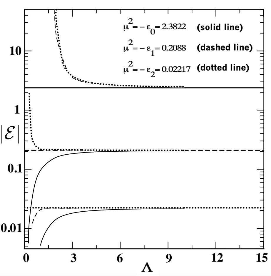
Figure 1: The convergence of the numerical results for the bound-state energies $\varepsilon$ is verified for the Hamiltonian given in Eq. (16), by considering our described renormalization procedure. The three exact energy eigenvalues are shown by the horizontal lines, as indicated. The same exact results are obtained, in the momentum cut-off limit $\Lambda\to\infty$, irrespectively to the values of the energy-scale parameter $-\mu^{2}$, which are used to renormalize the theory. The solid curves (converging to the first- and second-excited states) are given by assuming $\mu^{2}=2.3822$. The dashed curves (converging to ground and second-excited states) are for $\mu^{2}=0.2088$. The dotted curves (converging to ground and first-excited states) are for $\mu^{2}=0.02217$. All energy values ($\mu^{2}$, $\Lambda^{2}$ and $\varepsilon$) are in inverse-squared length units.

In Fig. 1, we are presenting the corresponding numerical results obtained for the eigenvalues of the Hamiltonian (16), as functions of the momentum cutoff parameter $\Lambda$. The three eigenvalue energies obtained by considering the reference regular potential (17) are shown by the three horizontal lines. As verified, the specific choice of the subtraction point $-\mu^{2}$ (one of the three values shown by the straight lines) does not affect the final convergent results, which are exact in the limit $\Lambda\to\infty$. The Fig. 1 displays three sets of results, such that, for each one, the value of $-\mu^{2}$ is specifically defined by one of the assumed known energies. Wth $\mu^{2}=$ $-\varepsilon^{(0)}=$ 2.3822, the results are given with solid lines for the first and second excited energies. In this case, the exact results obtained from Eq. (9) with $\Lambda\to\infty$ are $\varepsilon^{(1)}=-$0.2088 and $\varepsilon^{(2)}=-$0.02217. The results for the other two sets are obtained by using the same procedure: By assuming $\mu^{2}=$ $-\varepsilon^{(1)}=$ 0.2088, the results are with dashed lines; and when $\mu^{2}=$ $-\varepsilon^{(2)}=$ 0.02217, they are represented by dotted-lines. As verified, this diagonalization procedure provides stable results when $\Lambda\to\infty$, converging to the exact values, given by the real poles of the T-matrix: $\varepsilon^{(0)}=-$2.3822, $\varepsilon^{(1)}=-$0.2088 and $\varepsilon^{(2)}=-$0.02217.

As the renormalized Hamiltonian does not depend on the choice of $\mu$, it is a fixed-point Hamiltonian in this respect. The above example is providing a clear picture about what we have stated in Eq. (6). The momentum cutoff $\Lambda$ is just an instrumental regulator, which disappears as a natural infinite limit of the integrals, where all the infinities presented in the formalism are canceled out.

III.2 Four-term-singular renormalized Hamiltonian

A four-term-singular bare interaction is considered here in order to derive the explicit form of the renormalized potential, obtained for the $s-$wave after partial-wave decomposition. The matrix elements of this bare singular potential, in terms of powers of the momentum, is given by

$$\langle p|V|q\rangle=\sum_{i,j=0}^{1}\lambda_{ij}p^{2i}q^{2j}\;\;\;(\lambda_{ij}=\lambda_{ji}^{*})\ ,$$ (18)

with the renormalized strengths fixed by the physical scattering amplitude at a reference energy $-\overline{\mu}^{2}$,

$$\langle p|T(-{\overline{\mu}}^{2})|q\rangle=\lambda_{{\cal R}00}+\lambda_{{\cal R}10}(p^{2}+q^{2})+\lambda_{{\cal R}11}p^{2}q^{2}\ .$$ (19)

For simplicity, we assume that all strengths $\lambda_{{\cal R}ij}$ are real to have a Hermitian renormalized Hamiltonian. With the bare interaction given in (18), the physics of the system becomes completely defined by the values of the renormalized strengths, $\lambda_{{\cal R}ij}$, obtained at the reference energy $-\overline{\mu}^{2}$, which is also part of the physical input. Here, the units are $\hbar=m=1$, with $m$ the particle mass.

The potential given by Eq. (18) implies in integrals that diverge at most as $p^{5}$. In order to obtain finite integrals, this requires at least three subtractions in the kernel of the corresponding LS equation. With $n=3$ in Eq. (5), from the recurrence relationship (4), the following equations are derived:

$$\langle p|V^{(1)}(-\overline{\mu}^{2})|q\rangle=\lambda_{{\cal R}00},\quad\langle p|V^{(2)}(-\overline{\mu}^{2};k^{2})|q\rangle=\frac{1}{\lambda_{{\cal R}00}^{-1}+I_{0}},$$ (20)

$$\langle p|V^{(3)}(-\overline{\mu}^{2};k^{2})|q\rangle=\overline{\lambda}_{{\cal R}00}+\lambda_{{\cal R}10}(p^{2}+q^{2})+\lambda_{{\cal R}11}p^{2}q^{2},$$

where ${\overline{\lambda}}_{{\cal R}00}\equiv\left[{\lambda_{{\cal R}00}^{-1}+I_{0}+I_{1}}\right]^{-1},$ with $I_{i=0,1}\equiv I_{i}(k^{2},\overline{\mu}^{2})$ defined by

$$I_{i}(k^{2},\overline{\mu}^{2})\equiv\frac{2}{\pi}\int^{\infty}_{0}dqq^{2}\frac{(\overline{\mu}^{2}+k^{2})^{1+i}}{(\overline{\mu}^{2}+q^{2})^{2+i}}=\frac{(\overline{\mu}^{2}+k^{2})^{1+i}}{(2\overline{\mu})^{1+2i}}\ .$$ (21)

Note in above that the singular terms, as shown in Eq. (4), are introduced for $n=3$ in $V^{(3)}$. Also, we noticed that $I_{i}=0$ when $k^{2}=-\overline{\mu}^{2}$. By introducing $V^{(3)}(-\overline{\mu}^{2},k^{2})$ of Eq. (20) in Eq. (5), the renormalized interactions are obtained analytically, in this example, with the strenghts $\Lambda_{ji}(k^{2})$ not depending on the subtraction point, given by:

$$\langle p|V_{{\cal R}}|q\rangle=\sum_{i,j=0}^{1}\Lambda_{ij}(k^{2})p^{2i}q^{2j}\;\quad{\rm where}\quad[\Lambda_{ij}(k^{2})=\Lambda_{ji}(k^{2})]\quad{\rm with}$$ (22)

$$\Lambda_{00}(k^{2}) = \frac{\overline{\lambda}_{{\cal R}00}-\left(\overline{\lambda}_{{\cal R}00}K_{1}+\lambda_{{\cal R}10}K_{2}\right)\Lambda_{10}(k^{2})}{1+\overline{\lambda}_{{\cal R}00}K_{0}+\lambda_{{\cal R}10}K_{1}};\quad\Lambda_{11}(k^{2})=\frac{\lambda_{{\cal R}11}-\left(\lambda_{{\cal R}10}K_{0}+\lambda_{{\cal R}11}K_{1}\right)\Lambda_{10}(k^{2})}{1+\lambda_{{\cal R}11}K_{2}+\lambda_{{\cal R}10}K_{1}};$$

$$\Lambda_{10}(k^{2}) = \frac{\lambda_{{\cal R}10}+(\lambda_{{\cal R}10}^{2}-\overline{\lambda}_{{\cal R}00}\lambda_{{\cal R}11})K_{1}}{1+\overline{\lambda}_{{\cal R}00}K_{0}+\lambda_{{\cal R}10}K_{1}+\lambda_{{\cal R}11}K_{2}+\lambda_{{\cal R}10}K_{1}+(\lambda_{{\cal R}10}^{2}-\overline{\lambda}_{{\cal R}00}\lambda_{{\cal R}11})(K_{1}^{2}-K_{0}K_{2})},\;\;\;$$ (23)

where

$$K_{i=0,1,2} \equiv K_{i}(k^{2},{\overline{\mu}}^{2})\equiv\frac{2}{\pi}\int_{0}^{\infty}\frac{dqq^{2i+2}}{k^{2}-q^{2}}\left[1-\left(\frac{\overline{\mu}^{2}+k^{2}}{\overline{\mu}^{2}+q^{2}}\right)^{3}\right].$$ (24)

The $K_{i}$ are the divergent integrals, which cancel exactly the infinities of the LS equation obtained with the renormalized interaction (22). The integrands are given by the kernel of Eq. (5) with $n=3$.

In view of the arbitrariness of the subtraction point, the values of $\Lambda_{ij}(k^{2})$ are independent on the scale $\mu$, with ${\partial\Lambda_{ij}(k^{2})}/{\partial\mu^{2}}=0.$ These conditions on the derivatives are given by the explicit form of (6) in the case of the four-term-singular potential. However, the evolution of the driving term $V^{(3)}(-\mu^{2};k^{2})$ with $\mu$ can be computed by solving the first order differential CS equation (7) with the boundary condition at the initial scale $\mu^{2}=\overline{\mu}^{2}$. This would imply in a nontrivial dependence of the coefficients $\overline{\lambda}_{{\cal R}00}$, $\lambda_{{\cal R}10}$ and $\lambda_{{\cal R}11}$ with $\mu^{2}$ and $k^{2}$, which after all, will keep unchanged the $T-$matrix from the solution of the third-order subtracted scattering equation (3) using the new subtraction point.

III.3 Subtracted renormalization scheme for the one-pion-exchange potential

As a third pedagogical example, we consider here the application of the renormalization scheme, based on the subtracted T-matrix equation, to the neutron-proton system, with the basic formalism recovered from Ref. 1999fred , which was based in Weinberg’s pioneering work 1990wein . The subtraction parameter $\mu$ can run to infinite, which was indeed verified in the ³S${}_{1}-\,^{3}$D₁ and ³S₀ neutron-proton channels with the one-pion-exchange potential (OPEP) supplemented by contact interactions.

For the unregulated effective potential, in the corresponding matrix elements, a power expansion in the mid- and short-range parts of the interaction is usually assumed, in order to keep intact the well established long-range part of the OPEP. So, the matrix elements of the full effective nucleon-nucleon (ENN) interaction, with ${\vec{p}}-\vec{q}$ being the momentum transfer, can be expressed by

$$\langle{\bf p}|V_{ENN}|\vec{q}\rangle=\langle\vec{p}|V_{\pi}|\vec{q}\rangle + \frac{1}{2\pi^{2}}\left[\frac{1-\vec{\tau}_{1}\cdot\vec{\tau}_{2}}{4}\left(\lambda_{t}^{(0)}+\lambda_{t}^{(1)}q^{2}+\lambda_{t}^{(1)*}{p}^{2}+\cdot\cdot\cdot\right)+\right.$$ (25)

$$+ \left.\frac{3+\vec{\tau}_{1}\cdot\vec{\tau}_{2}}{4}\left(\lambda_{s}^{(0)}+\lambda_{s}^{(1)}q^{2}+\lambda_{s}^{(1)*}{p}^{2}+\cdot\cdot\cdot\right)\right],$$

with

$$\langle\vec{p}|V_{\pi}|\vec{q}\rangle=-\frac{g_{a}^{2}}{4(2\pi)^{3}f_{\pi}^{2}}\vec{\tau}_{1}\cdot\vec{\tau}_{2}\frac{\vec{\sigma}_{1}\cdot(\vec{p}-\vec{q})\;\vec{\sigma}_{2}\cdot(\vec{p}-\vec{q})}{(\vec{p}-\vec{q})^{2}+m_{\pi}^{2}}\ ,$$ (26)

where $\sigma_{i}$ and $\tau_{i}$ are the usual spin and isosping Pauli matrices for the nucleon $i=1,2$. The subindices $t$ and $s$ in the expansion strength parameters are for spin triplet (isospin singlet) and spin singlet (isospin triplet) channels, respectively. $g_{a}\;(=1.25)$ is the axial coupling constant, with $f_{\pi}\;(=93$ MeV) the pion weak-decay constant, with $m_{\pi}\;(=138$ MeV) the pion mass. By assuming only the leading order (LO) term of the expansion (25), we have $\lambda_{s(t)}^{(n)}=0$ for all $n\geq 1$.

Basically, it was applied in this case the same procedure as presented before, for the subtracted T-matrix formalism and for the renormalization of the interactions, with details also given in Ref. 1999fred . For that, only one scaling parameter $\mu$ was used, with the corresponding results showing an overall agreement with the neutron-proton data, particularly for the observables related to the triplet channel at low energies. The agreement is qualitative in the ¹S₀ channel. These results are shown in the four panels of Fig. 2. The mixing parameter for the ${}^{3}S_{1}-^{3}D_{1}$ states, considering the definition given in Ref. stapp , was verified to be the most sensible observable to the scale [see panel (d) of Fig. 2]. However, we should observe that the renormalization procedure, with just one subtraction and the triplet scattering length kept fixed, is enough to show a converged mixing parameter in the limit of $\mu\to\infty$, as panel (d) of Fig. 2 indicates.

With the renormalization group invariant approach for the subtraction procedure providing the basis on how to derive fixed-point Hamiltonians, this example was followed by a few other applications related to the OPEP, such as the corresponding procedure for the next-to-leading order (NLO) nucleon-nucleon interaction 2007tim . Within a more detailed methodology to renormalize the two nucleon interaction, with no need of cutoff regularization, by including more than one subtraction, better fits are provided for the nucleon-nucleon scattering observables in Ref. 2011tim .

In particular, we conclude this one-pion-exchange potential example, by observing that the applicability of the subtractive renormalization procedure can be further extended to cases in which higher order singularities exist in the interactions. By following the arguments of a similar approach developed in Ref. 2008bira , applied to renormalization of singular potentials containing divergences $1/r^{2}$ and $1/r^{4}$, one verifies that the present approach is perfectly suitable to the case in which we have the tensor part in spin-triplet channels of the one-pion-exchange interaction, which goes with $r^{-3}$ at the origin 2005Nogga , as the example shown in Fig. 2, where the OPEP in Eq. (26) includes such singularity. As also pointed out in Ref. 2011tim , the number of recursive steps required to renormalize the interaction depends on how the potential diverges, such that the method developed in Ref. 2000frederico can be implemented with a generic number of recursive steps or subtractions.

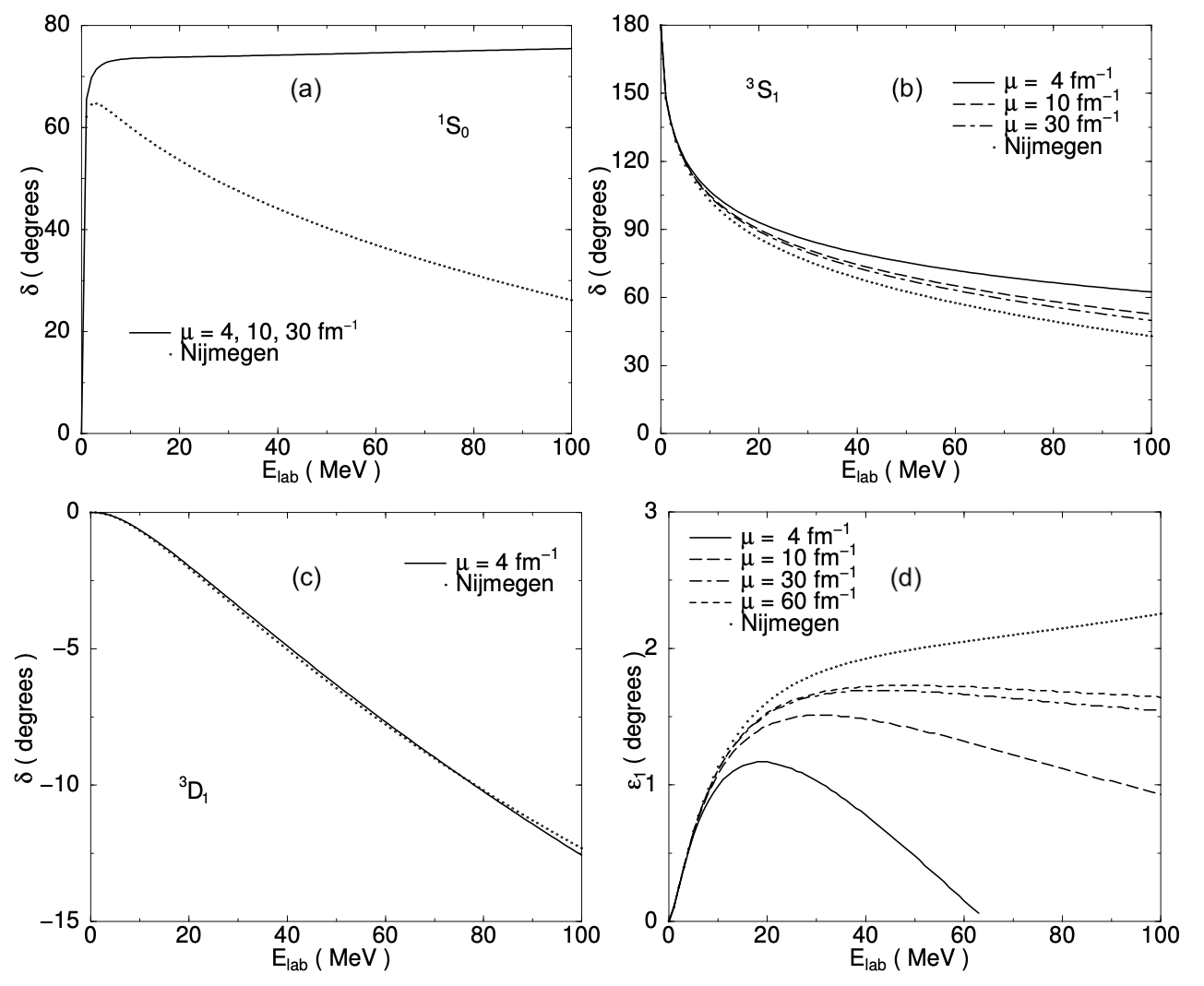
Figure 2: Neutron-Proton phase shifts for the ${}^{1}S_{0}$ state, $\delta_{0,s}$ [panel (a)]; ${}^{3}S_{1}$ state, $\delta_{0,t}$ [panel (b)]; ${}^{3}D_{1}$ state $\delta_{2,t}$ [panel (c)]; and mixing parameter for the ${}^{3}S_{1}-^{3}D_{1}$ states[panel (d)], according to Ref. stapp . The model results are shown for different values of $\mu$, as identified inside the panels. The dotted lines are data results from Ref. nij . These four-panel are extracted from plotted results presented in Ref. 1999fred . With more than one subtraction, see Ref. 2011tim .

IV Three-body subtracted equations with renormalized Hamiltonian

In this section, we review the derivation of the subtracted three-body Faddeev $T-$matrix equations proposed in 1995Adhikari1 and the renormalized Hamitonian, which contains two and three-body potentials. For a more detailed discussion, related to the subtracted formalism applied to three-body neutron-halo structures, which includes previous contributions, see Ref. 2012fred . A microscopic study of the trimer scaling function, within the perspective to be verified in cold-atom experiments, was done more recently in Ref. 2021madeira . Within the effective field theory (EFT), halo nuclei systems were also reviewed in HammerJPG2017 . In the scattering region, the neutron-deuteron scattering problem has been solved with a different form of subtracted equations AfnPRC2004 . The neutron-¹⁹C $s-$wave elastic scattering was studied in YamPLB2008b ; ShalchiPLB2017 . In atomic physics, the subtracted scattering equations were applied recently to different scattering problems, like the Efimov discrete scaling Efimov ; EfimovNPA1981 in an atom-molecule collision ShalchiPRA2018 and to study cold atom-dimer reaction rates with ⁴He, ^6,7Li, and ²³Na ShalchiPRA2020 . The application of subtracted equations to the four-boson problem with Dirac-delta interaction was proposed in Ref. YamEPL2006 , being further explored some years later leading to the discovery of a new four-boson limit cycle HadPRL2011 , independent of the Efimov discrete scaling.

IV.1 Subtracted Faddeev Equations

The subtraction method used to define the two-body T-matrix reviewed in section II was generalized to three-body systems. The subtracted Faddeev equations for the T-matrix 1995Adhikari1 were introduced in the context of a zero-range potential, although it can be generalized to account for potentials with a short-range term plus a Dirac-delta. The subtracted Faddeev equations follows the method applied to the two-body LS equation, where now the three-body free Green’s function in the kernel of the Faddeev integral equations are regularized by the subtraction $G_{0}(E)-G_{0}(-\mu_{3}^{2})$ substituting the free three-body Green’s function $G_{0}(E)$. As detailed in the case of the two-body problem, the advantage of using the subtracted T-matrix equations relies on its explicit renormalization group invariance, and the possibility of defining an associated renormalized Hamiltonian.

The three-body $T-$matrix at the subtraction point $-\mu_{3}^{2}$ is the sum of the two-body $T-$matrices for all the subsystems derived for singular potentials, which is given by

$$T(-\mu_{3}^{2})=\sum_{k=1,2,3}t_{(ij)}\left(-\mu_{3}^{2}-\frac{q_{k}^{2}}{2\;m_{ij,k}}\right),$$ (27)

where $k=1,2,3$ refers to one of the particles, with the remaining interacting pair $ij$ corresponding cyclically to $k$, as $ij=23,31,12$. For a given $k$, $m_{ij,k}$ is the associated reduced mass between this particle and the mass of the $ij-$pair $m_{i}+m_{j}$, given by $m_{ij,k}\equiv m_{k}(m_{i}+m_{j})/(m_{i}+m_{j}+m_{k})$. The two-body $T-$matrix $(t_{(ij)})$ is evaluated at the subsystem energy in the three-body center-of-mass.

The set of subtracted Faddeev equations, which have their detailed derivation in 2012fred , are given by:

$$T_{k}(E)=t_{(ij)}\left(E-\frac{q_{k}^{2}}{2m_{ij,k}}\right)\left[1+\left(G_{0}^{(+)}(E)-G_{0}(-\mu_{3}^{2})\right)\left(T_{i}(E)+T_{j}(E)\right)\right].$$ (28)

The solution of the homogeneous form of the above set of equations gives the bound-state energy, with the associated Faddeev component of the wave function vertex. In the case of the Dirac-delta potential the coupled set of equations is the regularized form 2012fred of the zero-range Skorniakov and Ter-Martirosian (SKTM) equation for the three-boson bound state Skorniakov1957 . When $\mu_{3}\to\infty$, we have the occurrence of the Thomas collapse ThomasPR1935 . However, for finite $\mu_{3}$ the scale invariance of the zero-range three-body T-matrix equation in the ultraviolet momentum region is broken and the Thomas collapse in the $s-$wave state of maximum symmetry does not happen. The correlations between three-body observables in this state tend to achieve a limit cycle, where the dependence on $\mu_{3}\to\infty$ does not matter and the theory in this sense is fully renormalized.

IV.2 Renormalized Three-body Hamiltonian

The renormalized three-body interaction Hamiltonian 2012fred , $H^{(3)}_{{\cal R}I}$, is obtained from Eq. (5). By resorting to one subtraction ($n=1$) where, at the subtraction point $-\mu_{3}^{2}$, we can identify $V^{(1)}$ with Eq. (27). From that, we can write the following equivalent equation:

$$H^{(3B)}_{{\cal R}I}=\sum_{k}\left[t_{(ij)}\left(-\mu_{3}^{2}-\frac{q^{2}_{k}}{2m_{ij,k}}\right)\right]\left(1-G_{0}(-\mu^{2}_{3})H^{(3B)}_{{\cal R}I}\right)\ .$$ (29)

The renormalized three-body interaction Hamiltonian (29) can be split in two- and three-body ones, by introducting the Faddeev decomposition of the three-body potential was introduced, as

$$H^{(3B)}_{{\cal R}I}=\sum_{k}\left[V^{(2B)}_{{\cal R}(ij)}+V^{(3B)}_{{\cal R}(k)}\right]\ ,$$ (30)

where, after formal manipulations, one gets the solution, which is given in matricial format as

$$\left[\begin{array}[]{ccc}1&V^{(2)}_{{\cal R}(23)}G_{0}(-\mu_{3}^{2})&V^{(2)}_{{\cal R}(23)}G_{0}(-\mu_{3}^{2})\\ V^{(2)}_{{\cal R}(31)}G_{0}(-\mu_{3}^{2})&1&V^{(2)}_{{\cal R}(31)}G_{0}(-\mu_{3}^{2})\\ V^{(2)}_{{\cal R}(12)}G_{0}(-\mu_{3}^{2})&V^{(2)}_{{\cal R}(12)}G_{0}(-\mu_{3}^{2})&1\end{array}\right]\left[\begin{array}[]{c}V^{(3)}_{{\cal R}(1)}+\\ V^{(3)}_{{\cal R}(2)}+\\ V^{(3)}_{{\cal R}(3)}+\end{array}\begin{array}[]{c}V^{(2)}_{{\cal R}(23)}\\ V^{(2)}_{{\cal R}(31)}\\ V^{(2)}_{{\cal R}(12)}\end{array}\right]=\left[\begin{array}[]{c}V^{(2)}_{{\cal R}(23)}\\ V^{(2)}_{{\cal R}(31)}\\ V^{(2)}_{{\cal R}(12)}\end{array}\right]\cdot$$ (43)

Note that $V^{(3B)}_{{\cal R}}$ is fully connected and contains the boundary condition at the subtraction point, Eq. (27), necessary for building the subtracted $T-$matrix equation for the three-body system. In the case of the Dirac-delta interaction, where one needs to solve the SKTM equations, the three-body renormalized potential allows its solution by introducing a subtraction in the kernel. This is the counterpart of the three-body potential necessary in the EFT approach (see, e.g., Ref. 2020ham ) to solve the SKTM equations. Therefore, the limit cycles and the scaling functions, which express correlations between three-body observables, obtained from the subtraction method, should agree with the corresponding approach derived from EFT applied to the three-body problem.

V Four-body scale and subtracted equations

The subtraction method used to define the two- an three-body T-matrix was also introduced in the Faddeev-Yakubovski (FY) formalism when considering four-particle systems with the Dirac-delta interactions in Ref. YamEPL2006 , which was followed by more detailed investigations by some of us in Refs. YamEPL2006 ; HadPRL2011 ; FredFBS2011 ; HadPRA2012 ; FredFBS2012 . In the four-bosons case, besides the three-body subtraction scaling point, another subtraction point has to be introduced, directly associated with the four-body scale, due to new terms in the FY coupled integral equations, which are not directly identified with the three-body kernel.

Next, we describe the main ideas concerned the application of the renormalization subtraction method, which was proposed in Ref. YamEPL2006 , to the four-body case. By considering the four particles identified by $i,j,k,l$ ranging from 1 to 4, the FY components of the wave function associated with the 3+1 partitions [$(ijk)+l,(jki)+l$ and $(kij)+l$], among the 18 possibilities, will fully describe the three-body subsystems $(ijk)$, such that, when the interaction with the fourth particle is turned off, the FY equations should reduce to the usual Faddeev three-body ones. With this reasoning, the subtracted form of the free Green’s function at the subtraction point $-\mu_{3}$ is introduced, as shown for the Faddeev equations (28). Physically, for the three-boson case, this subtraction point is associated with the necessity of an independent three-body scale to define the observables in the zero-range interaction limit, leading to limit cycles for the correlations between two observables of the three-boson S-wave state. Therefore, in the free Green’s function, which appears together with the FY components, associated to the three-body subsystem, it is adopted the energy subtraction at $-\mu_{3}^{2}$:

$$G_{0}(E)\longrightarrow G_{0}^{(3)}(E)\equiv G_{0}(E)-G_{0}(-\mu_{3}^{2}).$$ (44)

In principle, a different energy subtraction parameter $-\mu_{4}^{2}$, should emerge in the subtracted form of the Green’s functions coming together with the remaining fifteen FY components of the wave function. By following this reasoning, it was introduced in YamEPL2006 the subtraction of those Green’s function as:

$$G_{0}(E)\longrightarrow G_{0}^{(4)}(E)\equiv G_{0}(E)-G_{0}(-\mu_{4}^{2})\,.$$ (45)

This new subtraction would be irrelevant if one let $\mu_{4}\to\infty$ without consequences. However, it was observed in YamEPL2006 that the four-boson ground state collapses in this limit. Only in Ref. HadPRL2011 it was recognized that a new four-boson limit cycle occurs, which is being interwoven with the three-body Efimov limit cycle TomioFBS2014 . This limit cycle is associated with a new discrete scaling factor. It appears in the scaling function associated with the correlation between two consecutive tetramer energies at the unitary limit for a fixed trimer energy. The so-far results described here were also found consistent with the ones obtained in Ref. DeltuvaFBS2011 , which were obtained by considering finite-range potentials, corroborating the above analysis related to four-boson systems. By addressing general aspects of the universality in few-body systems, which include some discussion beyond three-body systems, we have already a few reviews which have appeared in the last decade, such as Refs. ZinnerJPG2013 ; NaidonRPP2017 ; GreeneRMP2017 .

The new four-boson limit-cycle has a discrete scaling which differs from the three-boson Efimov factor, corresponding to the breaking of the continuous scale symmetry to a discrete one verified in the FY zero-range equations FredFBS2019 . This brings together the necessity of a new four-boson scaling factor. The analytical derivation detailed in Ref. FredFBS2019 provides a discrete ratio different from the Efimov one, given by $s_{4}$, with the corresponding transcendental equation being such that the discrete ratio between the energies of successive tetramer states is given by $\rm{e}^{-2\pi/s_{4}}$, in the $\mu_{4}\to\infty$ limit for fixed trimer energy. This analysis, in which a four-boson scale emerges, being associated to a limit cycle, was further supported by the recent study in Ref. dePaulaJPG2020 , in which a system with $N$-light bosons and two heavy ones are considered within the Born-Oppenheimer approach. In this case, it was found that the strength of the attractive $1/r^{2}$ interaction depends on the number $N$ of light bosons, in correspondence to $s_{4}$. The study was done for the particular case in which the interactions (contact ones) can occur only between the light particles with the heavy ones. Therefore, in the case of the four-boson system, our expectation is that a four-body potential should emerge associated with the evolution of the system properties due to the new scale. However, providing an emergent universal behavior independent of the Efimov one.

Recently, it was demonstrated the necessity of the four-boson scale within the context of the EFT at NLO in Ref. BazakPRL2019 . Such finding should be reconciled with the breaking of the continuous scale symmetry of the FY equations to a discrete one in the limit of a zero-range potential, as expressed by the correlation found for the tetramer energies HadPRL2011 . The evolution along the correlation plot is implicitly governed by a four-body interaction, which would be in principle related to the subtraction in the FY equation, in this sense tuning the EFT four-body potential at NLO one eventually could find the trace of such correlation.

To close this section, we mention that other approaches have studied the universality and scaling in $N$-boson systems, with short-range interactions, as in Refs. GattobigioPRA2014 ; KievskyPRA2014 , where it was also considered the $N$-boson spectrum KievskyPRA2014 , without short-range four-boson forces, in which it was not possible to identify the dependence on the scales beyond the three-body one.

VI Conclusions

In summary, in this contribution to the memory of Steven Weinberg, we are reporting some works we have developed, which were mainly inspired in the fundamental contributions of Weinberg to the few-body physics, considering effective interactions among two- and three-nucleon systems. We start the report by considering the general ideas and works related to effective interactions which contains short-range singularities, from which concepts as universality and limit-cycles follow from the renormalization group approach. In section 2, we provide the basic formalism related to effective interactions, described by a Hamiltonian renormalization approach, which emerges as a consequence of a renormalization procedure, applied to the corresponding scattering matrix, at a fixed-point energy scale. The approach, shown to be renormalization group invariant, is based on a subtraction procedure, from which a fixed-point Hamiltonian can be derived. This renormalized Hamiltonian is taken as a fixed-point operator, in the sense that it does not depend on the position of the subtraction point $-\mu^{2}$, where the physical information is supplied to the theory. It naturally includes the renormalization group invariance properties of quantum mechanics with singular interactions, as expressed by the non-relativistic Callan-Symanzik equation. The theory is supplemented by three examples of applications to the case of two-particle systems, which have one or more singularities in their original interactions.

In section 4, we show how to apply the subtracted renormalization approach to three-body systems through the Faddeev formalism with singular two-body interactions. The section is concluded with some details on the possible extension to systems with four or more particles. The wide range of applicability of renormalized Hamiltonians, from atomic to nuclear physics models derived from effective theories of the QCD, is also emphasized in this section.

As a perspective, it would be of interest a comparison between the non-perturbative Hamiltonian renormalization approach, described in this report, with other available renormalization techniques applied to quantum few-body systems; such as, for example, the approach considered in Ref. birse . However, a caution is necessary when doing such comparison, as one should note that, in the present work, the invariance of the Hamiltonian is with respect to a subtraction energy scale, in the limit of infinite momentum cutoff. The present Hamiltonian renormalization approach is particularly useful when several discrete eigenvalues are possible, since it can be diagonalized, in a regularized form, in order to obtain physical observables that are well defined in the infinite cutoff limit.

Finally, inspired on the Weinberg effort to have a more comprehensible universe, besides his paradoxical conclusion that “The more the universe seems comprehensible, the more it seems pointless!”, let us make more understandable the quantum few-body physics with fixed-point Hamiltonians.

References

- (1) S. Weinberg, Phenomenological Lagrangians. Physica A 96, 327 (1979)
- (2) S. Weinberg, Nuclear forces from chiral Lagrangians. Phys. Lett. B 251, 288 (1990)
- (3) S. Weinberg, Effective chiral Lagrangians for nucleon-pion interactions and nuclear forces. Nucl. Phys. B 363, 3 (1991)
- (4) S. Weinberg, Three-body interactions among nucleons and pions. Phys. Lett. B 295, 114 (1992)
- (5) K. G. Wilson, Model of coupling-constant renormalization. Phys. Rev. D2, 1438 (1970
- (6) K. G. Wilson, Renormalization group and strong interactions. Phys. Rev. D 3, 1818 (1971)
- (7) K. G. Wilson and J. Kogut, The renormalization group and the expansion. Phys. Rep. 12 75, (1974)
- (8) K.G. Wilson, The renormalization group and critical phenomena. Rev. Mod. Phys.55, 583 (1983)
- (9) S.D. Glazek and K.G. Wilson, Renormalization of Hamiltonians. Phys. Rev. D48, 5863 (1993)
- (10) S. Glazek, A. Harindranath, S. Pinsky, J. Shigemitsu, and K. Wilson, Relativistic bound-state problem in the light-front Yukawa model. Phys. Rev. D 47 1599 (1993)
- (11) S. D. Glazek and K. G. Wilson, Perturbative renormalization group for Hamiltonians. Phys. Rev. D 49, 4214 (1994)
- (12) M.M. Brisudová, R.J. Perry and K.G. Wilson, Quarkonia in Hamiltonian Light-Front QCD. Phys.Rev. Lett. 78, 1227 (1997)
- (13) S. D. Glazek and K. G. Wilson Asymptotic freedom and bound states in Hamiltonian dynamics. Phys. Rev. D57, 3558 (1998)
- (14) S. Brodsky, H.-C. Pauli, S. Pinsky, Quantum chromodynamics and other field theories on the light cone. Phys. Rep. 301, 299 (1998)
- (15) G. P. Lepage, How to Renormalize the Schrödinger Equations, Proc. of the VIII Jorge André Swieca Summer School, pg.135, World Scientific, Singapore, 1997; nucl-th/9706029
- (16) S. D. Glazek and K. G. Wilson, Universality, marginal operators, and limit cycles. Phys. Rev. B 69, 094304 (2004)
- (17) A.E.A. Amorim, L. Tomio, and T. Frederico, Three-boson system with absorptive short range potential. Phys. Rev. C46, 2224 (1992)
- (18) A.E.A. Amorim, L. Tomio, and T. Frederico, Universal aspects of Efimov states and light halo nuclei. Phys. Rev. C56, 2378 (1997)
- (19) T. Frederico, L. Tomio, A. Delfino, and A.E.A. Amorim, Scaling limit of weakly bound triatomic states. Phys. Rev. A60, R9 (1999)
- (20) L. Tomio, T. Frederico, A. Delfino, and A.E.A. Amorim, Three helium atoms and the scaling limit. Few-Body Syst. Supp. 10, 203 (1999)
- (21) A. Delfino, T. Frederico and L. Tomio, Low-energy universality in three-body models. Few-Body Syst. 28, 259 (2000)
- (22) A. Delfino, T. Frederico, M.S.Hussein and L. Tomio, Virtual states of light non-Borromean halo nuclei. Phys. Rev. C 61, 051301 (2000)
- (23) T. Frederico, V.S. Timóteo, and L. Tomio, Renormalization of the one-pion-exchange interaction. Nucl. Phys. A 653, 209 (1999)
- (24) T. Frederico, A. Delfino and L. Tomio, Renormalization group invariance of quantum mechanics. Phys. Lett. B 481, 143 (2000)
- (25) V. Timóteo, T. Frederico, A. Delfino, and L. Tomio, Recursive renormalization of the singlet one-pion-exchange plus point-like interactions. Phys. Lett. B 621, 109 (2005)
- (26) V. S. Timóteo, T. Frederico, L. Tomio, and A. Delfino, Renomalization of the nn interaction at nnlo: uncoupled peripheral waves. Int. Jour. Mod. Phys. E 16, 2822 (2007)
- (27) V. Timóteo, T. Frederico, A. Delfino, and L. Tomio, Subtractive renormalization of the next-to-leading order NN interaction. Nucl. Phys. A 790, 406c (2007)
- (28) V. Timóteo, T. Frederico, A. Delfino, and L. Tomio, Nucleon-nucleon scattering within a multiple subtractive renormalization approach. Phys. Rev. C 83, 064005 (2011)
- (29) S. Szpigel, V. S. Timóteo and F. O. Durães, Similarity renormalization group evolution of chiral effective nucleon–nucleon potentials in the subtracted kernel method approach. Annals of Physics 326, 364 (2011)
- (30) S. Szpigel and V. S. Timóteo, Power counting and renormalization group invariance in the subtracted kernel method for the two-nucleon system. J. Phy. G: Nuclear and Particle Physics, 39, 105102 (2012)
- (31) M. C. Birse, The renormalization group and nuclear forces. Phil. Trans. R. Soc. A 369, 2662 (2011)
- (32) T. Frederico, A. Delfino, L. Tomio and M. T. Yamashita, Universal aspects of light halo nuclei. Prog. Part. Nucl. Phys. 67, 939 (2012)
- (33) E.F. Batista, S. Szpigel, V.S. Timóteo, Renormalization of Chiral Nuclear Forces with Multiple Subtractions in Peripheral Channels. Adv. High Energy Phys. 2017, 2316247 (2017)
- (34) H.-W. Hammer, S. König, and U. van Kolck, Nuclear effective field theory: Status and perspectives. Rev. Mod. Phys. 92, 025004 (2020)
- (35) E. Epelbaum, A. M. Gasparyan, J. Gegelia, Ulf-G. Meißner, X.-L. Ren, How to renormalize integral equations with singular potentials in effective field theory. Eur. Phys. J. A 56, 152 (2020)
- (36) E. F. Batista, S. Szpigel, V. S. Timóteo, Pions and Contacts at N4LO: Some details on the chiral nuclear force. Ann. of Phys. 425, 168383 (2021)
- (37) D. R. Entem and J. A. Oller, Non-perturbative methods for NN singular interactions. Eur. Phys. J. Spec. Top. 230, 1675 (2021)
- (38) V. S. Timóteo, Computational approaches for three-nucleon systems. Ann. of Phys. 432, 168573 (2021)
- (39) T. Frederico and H. C. Pauli, Renormalization of an effective light-cone QCD-inspired theory for the pion and other mesons. Phys. Rev. D 64 054007 (2001)
- (40) S. K. Adhikari, T. Frederico and I. D. Goldman, Perturbative Renormalization in Quantum Few-Body Problems. Phys. Rev. Lett. 74, 487 (1995)
- (41) S. K. Adhikari and T. Frederico, Renormalization Group in Potential Scattering. Phys. Rev. Lett. 74, 4572 (1995)
- (42) S. Weinberg, “The Quantum Theory of Fields Vol. I, Foundations”, Cambridge University Press 1995; and “The Quantum Theory of Fields Vol. II, Modern Applications”, Cambridge University Press, 1996
- (43) M. E. Fisher, Renormalization group theory: Its basis and formulation in statistical physics. Rev. Mod. Phys. 70, 653 (1998)
- (44) J. Zinn-Justin, Quantum Field Theory and Critical Phenomena, 4th ed., Claredon Press-Oxford 2002
- (45) C. G. Callan, Broken Scale Invariance in Scalar Field Theory. Phys. Rev. D2, 1541 (1970)
- (46) K. Symanzik, Renormalizable models with simple symmetry breaking. Comm. Math. Phys. 16, 48 (1970)
- (47) K. Symanzik, Small distance behaviour in field theory and power counting. Comm. Math. Phys. 18, 227 (1970)
- (48) H. Georgi, Effective field theory. Ann. Rev. Nucl. Part. Sc. 43, 209 (1993)
- (49) T. Frederico, A. Delfino, L. Tomio, and V.S. Timóteo, Fixed-Point Hamiltonians in Quantum Mechanics. arXiv:hep-ph/0101065 (2001)
- (50) H. P. Stapp, T. J. Ypsilantis, and N. Metropolis, Phase-shift analysis of 310-Mev proton-proton scattering experiments. Phys. Rev. 105, 302 (1957)
- (51) B. Long and U. van Kolck, Renormalization of singular potentials and power counting. Ann. of Phys. 323, 1304 (2008)
- (52) A. Nogga, R. G. E. Timmermans, and U. van Kolck, Renormalization of one-pion exchange and power counting, Phys. Rev. C 72, 054006 (2005)
- (53) V. G. J. Stocks, R. A. M. Klomp, C. P. F. Terheggen, and J.J. de Swart, Construction of high-quality NN potential models. Phys. Rev. C 49, 2950 (1994)
- (54) M. T. Yamashita, T. Frederico, L. Tomio, Neutron–19C scattering near an Efimov state. Phys. Lett. B 670, 49 (2008)
- (55) L. Madeira, T. Frederico, S. Gandolfi, L. Tomio, and M. T. Yamashita, Quantum Monte Carlo studies with microscopic two- and three-body interactions of a trimer scaling function. Preprint arXiv:2106.09058 (2021)
- (56) H.-W. Hammer, C. Ji, D. R. Phillips, Effective field theory description of halo nuclei. J. Phys. G 44, 10 (2017)
- (57) I. R. Afnan and D. R. Phillips, Three-body problem with short-range forces: Renormalized equations and regulator-independent results. Phys. Rev. C 69, 034010 (2004)
- (58) M. A. Shalchi, M. T. Yamashita, M. R. Hadizadeh, T. Frederico, L. Tomio, NeutronC scattering: Emergence of universal properties in a finite range potential. Phys. Lett. B 764, 196 (2017)
- (59) V. Efimov, Energy levels arising from resonant two-body forces in a three-body system. Phys. Lett. B 33, 563 (1970)
- (60) V. Efimov, Qualitative treatment of three-nucleon properties, Nucl. Phys. A, 362, 45 (1981)
- (61) M. A. Shalchi, M. T. Yamashita, M. R. Hadizadeh, E. Garrido, L. Tomio, and T. Frederico, Probing Efimov discrete scaling in an atom-molecule collision. Phys. Rev. A 97, 012701 (2018)
- (62) M. A. Shalchi, M. T. Yamashita, T. Frederico, L. Tomio, Cold atom-dimer reaction rates with 4He, 6,7Li, and 23Na. Phys. Rev. A 102, 062814 (2020)
- (63) M. T. Yamashita, L. Tomio, A. Delfino, T. Frederico, Four-boson scale near a Feshbach resonance. EPL 75, 555 (2006)
- (64) M. R. Hadizadeh, M. T. Yamashita, L. Tomio, A. Delfino, T. Frederico, Scaling properties of universal tetramers. Phys. Rev. Lett. 107, 135304 (2011)
- (65) G. V. Skorniakov and K. A. Ter-Martirosian, Three body problem for short range forces. I. Scattering of low en-ergy neutrons by deuterons. Soviet Phys. JETP 4, 648 (1957)
- (66) L. H. Thomas, The interaction between a neutron and a proton and the structure of H3. Phys. Rev. 47, 903 (1935)
- (67) T. Frederico, L. Tomio, A. Delfino, M. R. Hadizadeh, M. T. Yamashita, Scales and universality in few-body systems. Few-Body Syst. 51, 87 (2011)
- (68) M. R. Hadizadeh, M. T. Yamashita, L. Tomio, A. Delfino, T. Frederico, Binding and structure of tetramers in the scaling limit. Phys. Rev. A 85, 023610 (2012)
- (69) T. Frederico, A. Delfino, M. R. Hadizadeh, L. Tomio, and M. T. Yamashita, Universality in four-boson systems. Few-Body Syst. 54, 559 (2012)
- (70) L. Tomio, M. R. Hadizadeh, M. T. Yamashita, T. Frederico, A. Delfino, Trimer-tetramer interwoven states in the scaling limit. Few-Body Syst. 55, 949 (2014)
- (71) A. Deltuva, R. Lazauskas, and L. Platter, Universality in four-body scattering. Few-Body Syst. 51, 235 (2011)
- (72) N. T. Zinner and A. S. Jensen, Comparing and contrasting nuclei and cold atomic gases. J. Phys. G 40, 053101 (2013)
- (73) P. Naidon and S. Endo, Efimov Physics: a review. Rept. Prog. Phys. 80, 056001 (2017)
- (74) C. H. Greene, P. Giannakeas, and J. Perez-Rios, Universal few-body physics and cluster formation. Rev. Mod. Phys. 89, 035006 (2017)
- (75) T. Frederico, W. de Paula, A. Delfino, and M. T. Yamashita, L. Tomio, Four-boson continuous scale symmetry breaking. Few-Body Syst. 60, 46 (2019)
- (76) W. de Paula, A. Delfino, T. Frederico, and L. Tomio, Limit cycles in the spectra of mass imbalanced many-boson system. J. Phys. B 53, 205301 (2020)
- (77) B. Bazak, J. Kirscher, S. König, M. P. Valderrama, N. Barnea, and U. van Kolck, Four-body scale in universal few-boson systems. Phys. Rev. Lett. 122, 143001 (2019)
- (78) M. Gattobigio, A. Kievsky, Universality and scaling in the N-body sector of Efimov physics. Phys. Rev. A 90, 012502 (2014)
- (79) A. Kievsky, N. K. Timofeyuk, M. Gattobigio, N-boson spectrum from a discrete scale invariance. Phys. Rev. A 90, 032504 (2014)
- (80) M. C. Birse, J. A. McGovern, and K. G. Richardson, A renormalisation-group treatment of two-body scattering. Phys. Lett. B 464, 169 (1999)