Numerical modeling of anisotropic ferroelectric materials with hybridizable discontinuous Galerkin methods

Abstract.

We investigate a gradient flow structure of the Ginzburg–Landau–Devonshire (GLD) model for anisotropic ferroelectric materials by reconstructing its energy form. We show that the modified energy form admits at least one minimizer. Under some regularity assumptions for the electric charge distribution and the initial polarization field, we prove that the $L^{2}$ gradient flow structure has a unique solution. To simulate the GLD model numerically, we propose an energy-stable semi-implicit time stepping scheme and an hybridizable discontinuous Galerkin method for space discretization. Some numerical tests are provided to verify the stability and convergence of the proposed numerical scheme as well as some properties of ferrorelectric materials.

1. Introduction

1.1. Motivation

When designing a field–effect–transistor (FET) using Metal-Oxide-Semiconductors (MOSFET), one important task is to relax power density constraints in order to reduce the energy consumption of electronic devices. A typical measurement used to assess the performance of a MOSFET is given by the subthreshold swing (SS) value, i.e., the gate voltage value ($V_{g}$) which is necessary to vary the drain current ($I_{d}$) by ten times when it turns on or off. In conventional MOSFETs, where the conducting electrons are thermally injected over the potential barrier at the source/channel junction, the minimum theoretical SS value is 60mV/decade at room temperature, which is known as the Boltzmann tyranny. In most practical realizations, MOSFETs have a SS value closer to 70–90mv/decade, due to the presence of a gate insulator (GI) that absorbs a non-negligible part of the applied gate voltage and require higher voltages to modulate the channel conductance.

A promising solution proposed by Salahuddin and Datta (see [25]) consists in using GIs with negative capacitance (NC) transforming the GI into an internal voltage booster rather than a parasitic component. Salahuddin and Datta suggested using the depoled state of a ferroelectric (FE) thin film for such an internal voltage booster to decrease SS far below the Boltzmann limit; we refer to [22] for an introduction on the argument. In contrast to metal–ferroelectric–-insulator–semiconductor FET (MFISFET) memory devices, where the two distinguishable remnant polarization states of FE thin films are used to represent two memory states, NC mode operation requires a stable depoled state for the FE thin film in order to sustain the NC effect (see, e.g., [13]). As the MOSFET switching is a dynamic phenomenon, this has a significant implication for the low power operation because it allows a significantly decreased supply voltage for the device. In this paper, we are interested in the mathematical modeling of the polarization field in an FE material as well as its numerical simulations.

1.2. The GLD model

A conventional FET at a constant temperature can be modeled using a Poisson equation for the potential $V$ and a charge continuity equations (or drift diffusion equations) for electric and hole densities [19]. The polarization field ${\mathbf{P}}=(P_{1},\ldots,P_{d})^{\operatorname*{\intercal}}$ in the $d$-dimensional Euclidean space with $d\leq 3$ is usually modeled as an explicit function of the electric field ${\mathbf{E}}=-\nabla V$. For example, in dielectric or insulating materials, ${\mathbf{P}}=\epsilon_{0}\chi{\mathbf{E}}$, where $\epsilon_{0}$ is the permittivity of vacuum and $\chi$ is a function of the location. When considering FE materials, the potential needs to be remodeled together with the polarization. Here we apply the Ginzburg–Landau–Devonshire model [25]: given a device occupying the material domain $\Omega$, we want to find $V$ and ${\mathbf{P}}$ that minimize the following Gibbs free energy

(1) $$\widetilde{G}(V,{\mathbf{P}})=\int_{\Omega}\bigg{(}\rho V+{\mathbf{P}}\cdot\nabla V-\frac{\epsilon_{0}\epsilon_{b}}{2}|\nabla V|^{2}+F_{L}({\mathbf{P}})+F_{G}(\{P_{i,j}\})\bigg{)}\,\mbox{\rm d}x,$$

where $\rho$ is the electric charge distribution, $\epsilon_{b}$ is the relative background permittivity of the FE material and $g$ is the domain-wall coupling constant. $F_{L}({\mathbf{P}})$ is a Landau-type free-energy density functional and $F_{G}(\{P_{i,j}\})$ with $P_{i,j}=\partial_{x_{j}}P_{i}$ is a Ginzburg functional [12, 14, 21, 11]. For example, for the BaTiO₃-type FE materials, $F_{L}({\mathbf{P}})$ can be expanded with terms up to at least sixth order (cf. [9, 12]), namely,

$$F_{L}({\mathbf{P}}) =\alpha_{1}(P_{1}^{2}+P_{2}^{2}+P_{3}^{2})+\alpha_{11}(P_{1}^{4}+P_{2}^{4}+P_{3}^{4})$$

$$\qquad+\alpha_{12}(P_{1}^{2}P_{2}^{2}+P_{2}^{2}P_{3}^{2}+P_{1}^{2}P_{3}^{2})+\alpha_{111}(P_{1}^{6}+P_{2}^{6}+P_{3}^{6})$$

$$\qquad+\alpha_{112}[P_{1}^{4}(P_{2}^{2}+P_{3}^{2})+P_{2}^{4}(P_{1}^{2}+P_{3}^{2})+P_{3}^{4}(P_{1}^{2}+P_{2}^{2})]+\alpha_{123}P_{1}^{2}P_{2}^{2}P_{3}^{2},$$

and $F_{G}(\{P_{i,j}\})$ can be written as

$$F_{G}(\{P_{i,j}\}) =\frac{G_{1,1}}{2}(P_{1,1}^{2}+P_{2,2}^{2}+P_{3,3}^{2})$$

$$\qquad+G_{12}(P_{1,1}P_{2,2}+P_{2,2}P_{3,3}+P_{1,1}P_{3,3})$$

$$\qquad+\frac{G_{4,4}}{2}[(P_{1,2}+P_{2,1})^{2}+(P_{2,3}+P_{3,2})^{2}+(P_{3,1}+P_{1,3})^{2}].$$

Simple anisotropic FE materials

Some materials (such as HfO₂, cf. [15], see also [24, 13]) may be modeled as anisotropic FE materials, i.e., the FE behavior happens mostly along a certain axis and dielectric behavior is assumed for other axes. In such cases, we may model the total energy as

(2) $$G(V,{\mathbf{P}})=\int_{\Omega}\bigg{(}\rho V+{\mathbf{P}}\cdot\nabla V-\frac{\epsilon}{2}|\nabla V|^{2}+\sum_{i=1}^{d}(F(P_{i})+\frac{g_{i}}{2}|\nabla P_{i}|^{2})\bigg{)}\,\mbox{\rm d}x.$$

Here $F(P_{i}):=\alpha_{i}P_{i}^{2}+\beta_{i}P_{i}^{4}+\gamma_{i}P_{i}^{6}$, $\epsilon=\epsilon_{0}\epsilon_{b}$ and $\alpha_{i},\beta_{i},\gamma_{i}$ are FE anisotropic constants. In terms of the FE anisotropic constants, from what follows, we assume that for each $i=1,\ldots,d$,

• $P_{i}$ follows the dielectric property when $\alpha_{i}>0$ and $\beta_{i},\gamma_{i},g_{i}=0$ or

• $P_{i}$ follows the FE property when $\gamma_{i},g_{i}>0$ (e.g. [13]) or $\gamma_{i}=0$, $\beta_{i},g_{i}>0$ (e.g. [24, 15]).

Given a nanodevice occupying the region $\Omega$, we denote with $\Omega_{FE}\subset\Omega$ the domain of an FE material. Following [25], ${\mathbf{P}}$ vanishes in $\Omega\backslash\Omega_{FE}$. To simplify the treatment in this work, we set $\Omega_{FE}=\Omega$ so that the polarization field vanishes on $\partial\Omega$, the boundary of $\Omega$. In terms of boundary conditions for the potential, we set $\Gamma_{D}$ and $\Gamma_{N}$ to be disjoint subsets of $\partial\Omega$ such that $\Gamma_{D}\cup\Gamma_{N}=\partial\Omega$. We assume that $\Gamma_{D}\neq\emptyset$. For the simplicity of our discussion, we let the potential $V$ vanishes on $\Gamma_{D}$ and satisfying the following zero Neumann boundary condition on $\Gamma_{N}$:

$${\mathbf{D}}\cdot\nu:=(\epsilon{\mathbf{E}}+{\mathbf{P}})\cdot\nu=0,\quad\text{ on }\Gamma_{N}.$$

Here ${\mathbf{D}}$ is also referred to as the displacement field and $\nu$ denotes the outward normal vector. Noting that since ${\mathbf{P}}$ vanishes on $\partial\Omega$, the above Neumann boundary condition is also equivalent to

$${\mathbf{E}}\cdot\nu=0,\quad\text{ on }\Gamma_{N}.$$

1.3. Our contributions

We shall search for a minimizer of the Gibbs free energy $G(V,{\mathbf{P}})$ incorporate with the boundary conditions provided in the previous subsection. According to [18, 15] (see also [23] for a general framework), we only search for the minimizer along the path for $P_{i}$ when $P_{i}$ follows the FE property. More precisely speaking, we seek the solution $(V,{\mathbf{P}})$ satisfying ${\mathbf{P}}(t=0)={\mathbf{P}}_{0}$ and

(3) $$\delta_{V}G =0,$$

$$\delta_{P_{i}}G =0,\quad \text{ if }P_{i}\text{ follows the dielectric property},$$

$$\rho_{i}\partial_{t}P_{i} =-\delta_{P_{i}}G,\quad \text{ if }P_{i}\text{ follows the FE property}.$$

Here $\delta$ denotes the Frèchet derivative and $\rho_{i}>0$ is the viscosity constant. Motivated by [1] (see also [20] for the drift-diffusion system), we provide a modified energy form in Proposition 1 such that the corresponding $L^{2}$-gradient flow coincides with the system (3). Such energy form will help us construct stable numerical schemes approximating the minimizer. We further show in Proposition 2 that the minimization problem associated with the new energy form admits at least one minimizer.

We note that unlike the analysis for the classical Ginzburg–Landau system, or the Allen–Cahn equation (see e.g. [4, 10]), the polarization equation contains the coupling term $\nabla V$, which is a vector-valued function of ${\mathbf{P}}$ associated with the Poisson equation $\delta_{V}G=0$. To show the well-posedness of the weak form of the system (3), we utilize the energy estimates in [10] as well as the elliptic regularity for the Poisson equation. In Theorem 5, assuming that charge distribution $\rho$ is smooth enough, we prove that the weak solution exists if the initial polarization field is bounded in the energy space. Moreover, the weak solution is unique if $\Delta{\mathbf{P}}_{0}$ is bounded in the $L^{2}$ sense; see Theorem 7.

We next simulate an FE material by discretizing the problem (3). We shall first discretize the time derivative using the backward Euler method. In terms of computation of the nonlinear term in (3) for each time step, perhaps a proper treatment is to linearize the term by the Newton’s method (see e.g. [3, Algorithm 6.1.(iii)]). Such technique may lead to the time-stepping method conditionally stable with respect to $\rho_{i}$ and $g$, namely we may require that the time step $\tau\leq c\rho_{i}/g$ for some positive constant $c$. We may also need to guarantee that the discrete maximum principle holds, i.e., at each time step, the $L^{\infty}$ norm of the polarization field is uniformly bounded; see e.g. Proposition 6.6 of [3]. So it is not easy in practice to tune the time stepping scheme when simulating for different ferroelectric materials. In this work, we instead propose a semi-implicit scheme by splitting the gradient form provided in Proposition 1 with a convex and a concave part (see e.g. Chapter 6 of [3]). Such decomposition guarantees that the time-stepping method is unconditionally energy stable; see Proposition 9. Note that the nonlinear terms could be dominant during the evolution of the solutions. The fluxes for polarization field at the boundary could relatively large and thus create boundary layers. In order to capture these boundary layers in numerical simulations, a common strategy is to use discontinuous Galerkin methods to guarantee that (numerical) fluxes across faces of domain subdivisions are (weakly) continuous. Based on the time-stepping scheme, we consider a Hybridizable Discontinuous Galerkin Method (HDG) method which is originally proposed by [7]. One of advantages of HDG schemes is that even though the degrees of freedom are defined on both cells and faces of a subdivision of the material domain, due to the hybridization (or static condensation) property, the degrees of freedom on cells can be eliminated from the discrete system. Hence, the size of of discrete system to be solved for HDG discretization schemes is relatively smaller compared to regular discontinuous Galerkin schemes.

The rest of the paper is organized as follows. In Section 2, we provide a modified energy from for the weak form of (3) and show that the corresponding minimization problem admits at least one minimizer. We show the existence and uniqueness of the weak solution of (3) in Section 3. Section 4 provides a semi-implicit time discretization and an HDG space discretization scheme, respectively. Using our proposed numerical method, we present some convergence tests as well as numerical tests in a monolayer device in Section 5.

2. A minimization problem

In this section we consider a minimization problem derived from the energy form (2) and show that at least one minimizer exists. Let us first introduce some notations. Let $\Omega$ be a bounded domain with Lipschitz boundary. Given an integer $k\geq 0$ and a real number $p>1$, we denote $W^{k,p}(\Omega)$ the standard Sobolev space and we let $H^{k}(\Omega):=W^{k,2}(\Omega)$. Let ${\mathcal{V}}:=H^{1}_{0}(\Omega)$ be the subspace of $H^{1}(\Omega)$ whose functions vanishes at the boundary and

$$\mathcal{V}_{D}=\{w\in H^{1}(\Omega):w=0\text{ on }\Gamma_{D}\}.$$

Finally, we denote $(\cdot,\cdot)$ and $\|\cdot\|$ the $L^{2}(\Omega)$ inner product and the $L^{2}(\Omega)$ norm, respectively. For two vector fields ${\mathbf{P}},{\mathbf{Q}}\in[H^{1}(\Omega)]^{d}$, we set

$$(\nabla{\mathbf{P}},\nabla{\mathbf{Q}})=\sum_{i=1}^{d}(\nabla P_{i},\nabla Q_{i}).$$

Consider the following minimization problem: find $V\in{\mathcal{V}}_{D}$ and ${\mathbf{P}}\in[{\mathcal{V}}]^{d}$ so that

$$G(V,{\mathbf{P}})=\min_{\widetilde{V}\in{\mathcal{V}}_{D}\text{ and }\widetilde{\mathbf{P}}\in[{\mathcal{V}}]^{d}}G(\widetilde{V},\widetilde{\mathbf{P}}).$$

We shall search for a minimizer by solving its $L^{2}(\Omega)$ gradient flow. According to [15, 18], we additionally assume that the potential $V$ and certain components of the polarization field follow a dielectric behavior relax instantly in time, i.e., for the variational formulation, we have

(4) $$\delta_{V}G[w]=-(\epsilon\nabla V,\nabla w)+(\rho-\nabla\!{\cdot}{\mathbf{P}},w)=0,\quad{\text{ for all }}w\in{\mathcal{V}}_{D}$$

and

(5) $$\delta_{P_{i}}G[Q_{i}]=2\alpha_{i}(P_{i},Q_{i})+(\partial_{x_{i}}V,Q_{i})=0,\quad{\text{ for all }}Q_{i}\in{\mathcal{V}}.$$

We also point out that we have applied integration by parts $({\mathbf{P}},\nabla w)=-(\nabla\!{\cdot}{\mathbf{P}},w)$ in (4). For $P_{i}$ that follows the FE behavior, we have that

$$\rho_{i}\partial_{t}P_{i}=-\delta_{P_{i}}G[Q_{i}],\quad{\text{ for all }}Q_{i}\in\mathcal{V},$$

or

(6) $$\rho_{i}(\partial_{t}P_{i},Q_{i})+g_{i}(\nabla P_{i},Q_{i})+(DF(P_{i})P_{i},Q_{i})+(\partial_{x_{i}}V,Q_{i})=0.$$

Here $DF(P_{i})=2\alpha+4\beta P_{i}^{2}+6\gamma P_{i}^{4}$. The above equation is also referred to as the Landau-Khalatnikov equation [17].

2.1. A modified energy form

We shall reconstruct an energy form associated with the system (4)–(6). Given a polarization field ${\mathbf{P}}\in[{\mathcal{V}}]^{d}$, we consider the following energy functional

(7) $$I({\mathbf{P}})=\int_{\Omega}\bigg{(}\frac{\epsilon}{2}|\nabla{V_{{\mathbf{P}}}}|^{2}+F({\mathbf{P}})+\sum_{i=1}^{d}\frac{g_{i}}{2}|\nabla P_{i}|^{2}\bigg{)}\,\mbox{\rm d}x,$$

where $F({\mathbf{P}})=\sum_{i=1}^{d}F(P_{i})$ and ${V_{{\mathbf{P}}}}:=\Phi(\rho-\nabla\!{\cdot}{\mathbf{P}})$ with $\Phi:L^{2}(\Omega)\to{\mathcal{V}}$ denoting the solution operator so that for $g\in L^{2}(\Omega)$, $\Phi g$ uniquely solves

(8) $$(\epsilon\nabla\Phi g,\nabla w)=(g,w),\quad{\text{ for all }}w\in{\mathcal{V}}_{D}.$$

So $V={V_{{\mathbf{P}}}}$ in (4).

Proposition 1.

We have $I({\mathbf{P}})=G({V_{{\mathbf{P}}}},{\mathbf{P}})$ and the corresponding $L^{2}(\Omega)$ gradient flow coincides with (4)–(6) by setting $V={V_{{\mathbf{P}}}}$. In particular,

(9) $$\rho_{i}\partial_{t}P_{i}=-\delta_{P_{i}}I({\mathbf{P}}),$$

with $\rho_{i}=0$ if $P_{i}$ follows the dielectric property and $\rho_{i}>0$ if $P_{i}$ follows the FE property.

Proof.

Choosing $w={V_{{\mathbf{P}}}}$ in (4) we get

$$\int_{\Omega}\frac{\epsilon}{2}|\nabla{V_{{\mathbf{P}}}}|^{2}\,\mbox{\rm d}x=\int_{\Omega}\rho{V_{{\mathbf{P}}}}+{\mathbf{P}}\cdot\nabla{V_{{\mathbf{P}}}}-\frac{\epsilon}{2}|\nabla{V_{{\mathbf{P}}}}|^{2}\,\mbox{\rm d}x.$$

This implies that $I({\mathbf{P}})=G({V_{{\mathbf{P}}}},{\mathbf{P}})$ according to (2). To obtain the gradient flow from $I({\mathbf{P}})$, it suffices to show that the differential of ${\mathbf{P}}\cdot\nabla{V_{{\mathbf{P}}}}$ is $\nabla{V_{{\mathbf{P}}}}$. Letting $H(g)=\tfrac{\epsilon}{2}\int_{\Omega}|\nabla\Phi g|^{2}\,\mbox{\rm d}x$, Lemma 6.1 of [1] implies that $\delta_{g}H(g)[w]=(\Phi g,w)$, with $w\in{\mathcal{V}}$. So given ${\mathbf{Q}}\in[C^{\infty}_{0}(\Omega)]^{d}$,

$$H(\rho-\nabla\!{\cdot}({\mathbf{P}}+{\mathbf{Q}})) -H(\rho-\nabla\!{\cdot}{\mathbf{P}})$$

$$=\delta_{g}H(\rho-\nabla\!{\cdot}{\mathbf{P}})[-\nabla\!{\cdot}{\mathbf{Q}}]+O(\|\nabla\!{\cdot}{\mathbf{Q}}\|)$$

$$=-({V_{{\mathbf{P}}}},\nabla\!{\cdot}{\mathbf{Q}})+O(\|\nabla\!{\cdot}{\mathbf{Q}}\|).$$

Using integration by parts for the first term on the right hand side above, we conclude that $\delta_{\mathbf{P}}H(\rho-\nabla\!{\cdot}{\mathbf{P}})[{\mathbf{Q}}]=(\nabla{V_{{\mathbf{P}}}},{\mathbf{Q}})$, as desired. ∎

2.2. Existence of minimizers

We shall apply the direct method in the calculus of variation to show that the following minimization problem

(10) $$I({\mathbf{P}})=\min_{\tilde{\mathbf{P}}\in[{\mathcal{V}}]^{d}}I(\tilde{\mathbf{P}})$$

has at least one minimizer.

Weakly lower semicontinuity for the higher order terms

Let us first verify that

$$\int_{\Omega}\bigg{(}\frac{\epsilon}{2}|\nabla{V_{{\mathbf{P}}}}|^{2}+\sum_{i=1}^{d}\frac{g_{i}}{2}|\nabla P_{i}|^{2}\bigg{)}\,\mbox{\rm d}x$$

is weakly lower semicontinuous and $I({\mathbf{P}})$ is coercive. It is well known that the second term above is weakly lower semicontinuous (see e.g., [3, Example 2.1]). Here we check for $\int_{\Omega}\frac{\epsilon}{2}|\nabla V_{{\mathbf{P}}}|^{2}$. Let $\{{\mathbf{P}}_{n}\}_{n\in\mathbb{N}}$ be a sequence in $[{\mathcal{V}}]^{d}$ such that ${\mathbf{P}}_{n}$ weakly converges to ${\mathbf{P}}$ in $[{\mathcal{V}}]^{d}$. Note that

$$\int_{\Omega}\frac{\epsilon}{2}|\nabla V_{{\mathbf{P}}}|^{2}\,\mbox{\rm d}x-\int_{\Omega}\frac{\epsilon}{2}|\nabla V_{{\mathbf{P}}_{n}}|^{2}\,\mbox{\rm d}x+\int_{\Omega}\frac{\epsilon}{2}|\nabla({V_{{\mathbf{P}}}}-V_{{\mathbf{P}}_{n}})|^{2}\,\mbox{\rm d}x$$

$$\quad\quad\quad\quad=\int_{\Omega}\epsilon\nabla{V_{{\mathbf{P}}}}\cdot\nabla({V_{{\mathbf{P}}}}-V_{{\mathbf{P}}_{n}})\,\mbox{\rm d}x=\int_{\Omega}({\mathbf{P}}-{\mathbf{P}}_{n})\cdot\nabla{V_{{\mathbf{P}}}}\,\mbox{\rm d}x,$$

where we applied (4) for both ${V_{{\mathbf{P}}}}$ and $V_{{\mathbf{P}}_{n}}$ in the last equality above. Letting $n\to\infty$ yields

$$\int_{\Omega}\frac{\epsilon}{2}|\nabla{V_{{\mathbf{P}}}}|^{2}\,\mbox{\rm d}x\leq\liminf_{n\to\infty}\int_{\Omega}\frac{\epsilon}{2}|\nabla V_{{\mathbf{P}}_{n}}|^{2}\,\mbox{\rm d}x.$$

Coercivity

Note for both properties of $P_{i}$, the polynomial $F(P_{i})$ has a minimum $-c_{0}$ with $c_{0}\geq 0$. Suppose there is a sequence $\{{\mathbf{P}}_{n}\}_{n=1}^{\infty}\subset[{\mathcal{V}}]^{d}$ with $\|{\mathbf{P}}_{n}\|_{H^{1}(\Omega)}\to\infty$. We have

(11) $$\int_{\Omega}F({\mathbf{P}}_{n})\,\mbox{\rm d}x\geq-dc_{0}|\Omega|.$$

Whence,

(12) $$I({\mathbf{P}}_{n})\geq\frac{g}{2}\|\nabla{\mathbf{P}}_{n}\|^{2}-dc_{0}|\Omega|\to\infty,\quad\text{ as }n\to\infty$$

as $n\to\infty$. This implies that $I({\mathbf{P}})$ is coercive.

Existence of the minimizer

Now we are ready to show the existence of a minimizer for the problem (10).

Proposition 2 (existence of a minimizer).

Given an FE material occupying the domain $\Omega$, let $c_{0}$ be defined as in (11). Then there exists at least one minimizer for problem (10).

Proof.

In view of (12), $I({\mathbf{P}})$ is also bounded below. So there exists a sequence $\{{\mathbf{P}}_{n}\}_{n=1}^{\infty}\subset[{\mathcal{V}}]^{d}$ such that $\lim_{n\to\infty}I({\mathbf{P}}_{n})=\inf_{\widetilde{\mathbf{P}}\in[{\mathcal{V}}]^{d}}I(\widetilde{\mathbf{P}})$. The coercivity of $I({\mathbf{P}})$ (cf. (12)) implies that ${\mathbf{P}}_{n}$ is bounded in $[{\mathcal{V}}]^{d}$ so there exists a subsequence of $\{{\mathbf{P}}_{n}\}$ weakly converging to some limit ${\mathbf{P}}$ in $[{\mathcal{V}}]^{d}$. Here without loss of generality, we denote this subsequence by $\{{\mathbf{P}}_{n}\}$. Due to the lower semicontinuity of the higher order term in $I({\mathbf{P}})$, we have

$$\int_{\Omega}\frac{\epsilon}{2}|\nabla{V_{{\mathbf{P}}}}|^{2}+\sum_{i=1}^{d}\frac{g_{i}}{2}|\nabla P_{i}|^{2}\,\mbox{\rm d}x\leq\liminf_{n\to\infty}\int_{\Omega}\frac{\epsilon}{2}|\nabla V_{{\mathbf{P}}_{n}}|^{2}+\sum_{i=1}^{d}\frac{g_{i}}{2}|\nabla P_{ni}|^{2}\,\mbox{\rm d}x,$$

with $P_{ni}$ denoting the $i$-th component of ${\mathbf{P}}_{n}$. On the other hand, by the compactly embedding from ${\mathcal{V}}$ into $L^{6}(\Omega)$ for $d=1,2,3$, $\{{\mathbf{P}}_{n}\}$ (again, w.l.o.g. by passing to a subsequence) also strongly converges to ${\mathbf{P}}$ in $L^{6}(\Omega)$. So

$$\int_{\Omega}F({\mathbf{P}}_{n})\,\mbox{\rm d}x\to\int_{\Omega}F({\mathbf{P}})\,\mbox{\rm d}x,\quad\text{ as }n\to\infty.$$

Combing the above two limits implies that

$$I({\mathbf{P}})\leq\liminf_{n\to\infty}I({\mathbf{P}}_{n})=\lim_{n\to\infty}I({\mathbf{P}}_{n})=\inf_{\widetilde{\mathbf{P}}\in[{\mathcal{V}}]^{d}}I(\widetilde{\mathbf{P}}).$$

Since $I({\mathbf{P}})\geq\inf_{\widetilde{\mathbf{P}}\in[{\mathcal{V}}]^{d}}I(\widetilde{\mathbf{P}})$ by definition, we conclude that ${\mathbf{P}}$ is a minimizer of the problem (10). ∎

Remark 3 ((uniqueness)).

It is sufficient to show that there exists at most one minimizer when $I(P)$ is strictly convex. We note that $\int_{\Omega}|\nabla{V_{{\mathbf{P}}}}|^{2}$ is convex with respect to ${\mathbf{P}}$. Indeed, as $\int_{\Omega}|\nabla V|^{2}$ is convex for $V$, we have for ${\mathbf{P}}_{1},{\mathbf{P}}_{2}\in[{\mathcal{V}}]^{d}$ and $\lambda\in[0,1]$,

$$\lambda\int_{\Omega}|\nabla V_{{\mathbf{P}}_{1}}|^{2}\,\mbox{\rm d}x +(1-\lambda)\int_{\Omega}|\nabla V_{{\mathbf{P}}_{2}}|^{2}\,\mbox{\rm d}x$$

$$\geq\int_{\Omega}|\nabla(\lambda V_{{\mathbf{P}}_{1}}+(1-\lambda)V_{{\mathbf{P}}_{2}})|^{2}\,\mbox{\rm d}x$$

$$=\int_{\Omega}|\nabla\Phi(\rho-\nabla\!{\cdot}(\lambda{\mathbf{P}}_{1}+(1-\lambda){\mathbf{P}}_{2}))|^{2}\,\mbox{\rm d}x$$

$$=\int_{\Omega}|\nabla V_{\lambda{\mathbf{P}}_{1}+(1-\lambda)V_{{\mathbf{P}}_{2}}}|^{2}\,\mbox{\rm d}x,$$

recalling that the linear operator $\Phi$ is defined in (8). However, we cannot guarantee the convexity due to choice of the constants $\alpha_{i},\beta_{i},\gamma_{i}$ inside the Landau-type density functional $\int_{\Omega}F(P_{i})$. Considering the second derivative of $F(P_{i})$, a sufficient condition for uniqueness is that for each component $P_{i}$ following the FE property, the quadratic form $p(t)=30\gamma_{i}t^{2}+12\beta_{i}t+2\alpha_{i}$ is strictly positive for $t>0$. This leads to the following two conditions:

• $\alpha_{i},\beta_{i}>0$ or

• $\gamma_{i}>0$, $\beta_{i}<0$ and $3\beta_{i}^{2}/(5\gamma_{i})<\alpha_{i}$.

3. Well-posedness of the gradient flow

This section is devoted to showing the existence and uniqueness of the weak solution to the $L^{2}$ gradient flow (4)–(6). For simplicity, we assume that all components of the polarization field follow the FE property with the same constants denoting by $\rho,\alpha,\beta,\gamma$ and $g$. To discuss the well-posedness, we shall introduce the Bochner-Sobolev spaces. Given a Banach space $B$, $r\geq 1$ and a final time $T$, the space $L^{r}(0,T;B)$ is a collection of functions so that for each $w\in L^{r}(0,T;B)$, the norm

$$\|w\|_{L^{r}(0,T;B)}=\left\{\begin{aligned} &\bigg{(}\int_{0}^{T}\|w\|_{B}^{r}\,\mbox{\rm d}t\bigg{)}^{1/r},&&\quad r\in[1,\infty),\\ &\text{esssup}_{t\in[0,T]}\|w\|_{B},&&\quad r=\infty,\end{aligned}\right.$$

is finite. We also define the space $H^{1}(0,T;B)$ by

$$H^{1}(0,T;B):=\{u\in L^{2}(0,T;B):\partial_{t}u\in L^{2}(0,T;B)\}.$$

Denote ${\mathcal{V}}^{\prime}$ the dual space of ${\mathcal{V}}$ and let $\langle\cdot,\cdot\rangle$ the corresponding duality pairing. A weak formulation of problem (4)–(6) reads: given an initial polarization ${\mathbf{P}}_{0}$ and a final time $T$, we want to find ${\mathbf{P}}:={\mathbf{P}}(t)\in L^{2}(0,T;[{\mathcal{V}}]^{d})\cap H^{1}(0,T;[{\mathcal{V}}^{\prime}]^{d})$ such that ${\mathbf{P}}(0)={\mathbf{P}}_{0}$ and

(13) $$\rho_{v}\langle\partial_{t}{\mathbf{P}},{\mathbf{Q}}\rangle+g(\nabla{\mathbf{P}},\nabla{\mathbf{Q}})$$

$$\quad\quad+(\mathbf{D}F({\mathbf{P}}),{\mathbf{Q}})+(\nabla{V_{{\mathbf{P}}}},{\mathbf{Q}})=0,\quad{\text{ for all }}{\mathbf{Q}}\in[{\mathcal{V}}]^{d}\text{ and }t\in(0,T],$$

where ${V_{{\mathbf{P}}}}$ is given by (7) and $\mathbf{D}F({\mathbf{P}})=(DF(P_{i})P_{i})_{i=1}^{d}$. Here we also note that for simplicity of our discussion, we set the viscosity constant $\rho_{v}=\rho_{i}$ for $i=1,\ldots,d$.

3.1. Existence

Thanks to Fredholm alternative, there exist $L^{2}(\Omega)$-orthonormal eigenfunctions $\{\phi_{i}\}_{i=1}^{\infty}$ with increasing eigenvalues $\{\lambda_{i}\}_{i=1}^{\infty}\subset(0,\infty)$ satisfying

$$(\nabla\phi_{i},\nabla w)=\lambda_{i}(\phi_{i},w),\quad{\text{ for all }}w\in{\mathcal{V}}.$$

Given a positive integer $N$, set $X_{N}=\text{span}\{\phi_{i}\}_{i=1}^{N}$ and we consider the following finite dimensional problem: find ${\mathbf{P}}_{N}(t)\in[X_{N}]^{d}$ such that

(14) $$\rho_{v} \langle\partial_{t}{\mathbf{P}}_{N},{\mathbf{Q}}\rangle+g(\nabla{\mathbf{P}}_{N},\nabla{\mathbf{Q}})$$

$$+(\mathbf{D}F({\mathbf{P}}_{N}),{\mathbf{Q}})+(\nabla V_{{\mathbf{P}}_{N}},{\mathbf{Q}})=0, {\text{ for all }}{\mathbf{Q}}\in[X_{N}]^{d}\text{ and }t\in(0,T],$$

$$({\mathbf{P}}_{N}(0),{\mathbf{Q}})=({\mathbf{P}}_{0},{\mathbf{Q}}), {\text{ for all }}{\mathbf{Q}}\in[X_{N}]^{d}.$$

We first note that if the charge distribution $\rho\in L^{\infty}(0,T;L^{2}(\Omega))$, the above problem has a solution. This can be shown by exploiting the fact that $\mathbf{D}F$ is a bounded operator in $[X_{N}]^{d}$ equipped with $[L^{2}(\Omega)]^{d}$ norm. Here we sketch one approach of the proof: one can derive that $\delta_{{\mathbf{P}}}I({\mathbf{P}})[{\mathbf{Q}}]$ is bounded and semicoercive, namely there exist positive constants $C,C_{1},C_{2},C_{3}$ so that

$$\delta_{{\mathbf{P}}}I({\mathbf{P}}_{N})[{\mathbf{Q}}]\leq C(\|{\mathbf{P}}_{N}\|+\|\nabla{\mathbf{P}}_{N}\|+\|\rho\|)\|{\mathbf{Q}}\|_{[{\mathcal{V}}]^{d}}$$

and

$$\delta_{{\mathbf{P}}}I({\mathbf{P}}_{N})[{\mathbf{P}}_{N}]\geq C_{1}\|\nabla{\mathbf{P}}_{N}\|^{2}-C_{2}\|{\mathbf{P}}_{N}\|^{2}-C_{3}\|\rho\|^{2}.$$

Since $I({\mathbf{P}})$ is semicoercive and weakly lower semicontinuous, we can follow the argument from [3, Section 2.3] to show the existence of ${\mathbf{P}}_{N}$. That is constructing a solution of ${\mathbf{P}}_{N}$ by an approximation using the backward Euler scheme.

We next provide some auxiliary estimates related to ${\mathbf{P}}_{N}$. From what follows, we use $C$ to denote a generic constant independent of $N$.

Lemma 4.

Suppose that the initial polarization field ${\mathbf{P}}_{0}\in[H^{1}(\Omega)\cap L^{\infty}(\Omega)]^{d}$ and the charge distribution $\rho\in H^{1}(0,T;L^{2}(\Omega))$. Then for a fixed final time $T$, there holds:

1. ${\mathbf{P}}_{N}\in L^{\infty}(0,T;[L^{2}(\Omega)]^{d})\cap L^{2}(0,T;[{\mathcal{V}}]^{d})$ and $V_{{\mathbf{P}}_{N}}\in L^{2}(0,T;{\mathcal{V}}_{D})$, i.e., there exists a positive constant $C$ independent of $N$ satisfying

   $$\max_{t\in[0,T]}\|{\mathbf{P}}_{N}(t)\|^{2}+\int_{0}^{T}\|\nabla{\mathbf{P}}_{N}(t)\|^{2}+\|{\mathbf{P}}_{N}(t)\|^{2}+\|\nabla V_{{\mathbf{P}}_{N}}(t)\|^{2}\,\mbox{\rm d}t\leq C.$$

2. Assume that we have the $H^{2}(\Omega)$ elliptic regularity in (8), i.e., for $g\in L^{2}(\Omega)$,

   $$\|\Phi g\|_{H^{2}(\Omega)}\leq C\|g\|,$$

   where the constant $C$ only depends on $d$ and $\Omega$. Then ${\mathbf{P}}_{N}\in H^{1}(0,T;L^{2}(\Omega))$. More precisely,

   $$I({\mathbf{P}}_{N}(T))+\rho_{v}\int_{0}^{T}\|\partial_{t}{\mathbf{P}}_{N}(t)\|^{2}\,\mbox{\rm d}t\leq I({\mathbf{P}}_{0})+\frac{1}{2}\int_{0}^{T}\|\rho_{t}(t)\|^{2}+\|V_{{\mathbf{P}}_{N}}(t)\|^{2}\,\mbox{\rm d}t.$$

3. There exists a positive constant $C$ independent of $N$ such that

   $$\int_{0}^{T}\|\Delta{\mathbf{P}}_{N}(t)\|^{2}\,\mbox{\rm d}t\leq C\int_{0}^{T}\|\nabla{\mathbf{P}}_{N}(t)\|^{2}+\|\partial_{t}{\mathbf{P}}_{N}(t)\|^{2}+\|\rho(t)\|^{2}\,\mbox{\rm d}t.$$

   Under the assumption in part (b), we conclude that ${\mathbf{P}}_{N}$ is uniformly bounded in $L^{2}(0,T;H^{2}(\Omega))$.

Proof.

$$1$$ To prove (a), we let ${\mathbf{Q}}={\mathbf{P}}_{N}$ in (14) to get that for any $\mu>0$,

$$\frac{\rho_{v}}{2}\,\mbox{\rm d}_{t}\|{\mathbf{P}}_{N}(t)\|^{2} +g\|\nabla{\mathbf{P}}_{N}(t)\|^{2}+\epsilon\|\nabla V_{{\mathbf{P}}_{N}}(t)\|^{2}$$

$$=(\rho,V_{{\mathbf{P}}_{N}})+c_{1}\|{\mathbf{P}}_{N}(t)\|^{2}$$

$$\leq\frac{\mu C_{p}^{2}}{2}\|\nabla V_{{\mathbf{P}}_{N}}\|^{2}+\frac{1}{2\mu}\|\rho\|^{2}+c_{1}\|{\mathbf{P}}_{N}(t)\|^{2},$$

where we used the facts that $DF(P_{i})=2\alpha+4\beta P_{i}^{2}+6\gamma P_{i}^{4}\geq-c_{1}$ for some $c_{1}\geq 0$ and $(\nabla V_{{\mathbf{P}}_{N}},{\mathbf{P}}_{N})=\epsilon\|\nabla V_{{\mathbf{P}}_{N}}\|^{2}-(\rho,V_{{\mathbf{P}}_{N}})$ according to (4). We also note that for the last inequality above, we applied the Schwarz inequality as well as the Poincaré inequality with $C_{p}$ denoting the Poincaré constant. Now we set $\mu=\epsilon/C_{p}^{2}$ and integrate the above inequality over $[0,T]$ to obtain that

$$\|{\mathbf{P}}_{N}(T)\|^{2} \leq\|{\mathbf{P}}_{N}(T)\|^{2}+\frac{2}{\rho_{v}}\int_{0}^{T}g\|\nabla{\mathbf{P}}_{N}(t)\|^{2}+\frac{\epsilon}{2}\|\nabla V_{{\mathbf{P}}_{N}}\|^{2}\,\mbox{\rm d}t$$

$$\leq\|{\mathbf{P}}(0)\|^{2}+\frac{2}{\rho_{v}}\int_{0}^{T}c_{1}\|{\mathbf{P}}_{N}(t)\|^{2}+\frac{C_{p}^{2}}{2\epsilon}\|\rho(t)\|^{2}\,\mbox{\rm d}t.$$

Gröwall’s inequality implies that $\max_{t\in[0,T]}\|{\mathbf{P}}_{N}(t)\|^{2}\leq C$. Applying this estimate to the second inequality above implies that

$$\int_{0}^{T}\|\nabla{\mathbf{P}}_{N}(t)\|^{2}+\|\nabla V_{{\mathbf{P}}_{N}}(t)\|^{2}\,\mbox{\rm d}t\leq C.$$

Then,

(15) $$\int_{0}^{T}\|{\mathbf{P}}_{N}(t)\|^{2}\,\mbox{\rm d}t\leq C\int_{0}^{T}\|\nabla{\mathbf{P}}_{N}(t)\|^{2}\,\mbox{\rm d}t\leq C$$

due to the Poincaré inequality.

$$2$$ Before showing the estimate (b), we note that $V_{{\mathbf{P}}_{N}}\in H^{2}(\Omega)$ due to the elliptic regularity assumption and hence $V_{{\mathbf{P}}_{N}}$ satisfies the equation

$$-\epsilon\Delta V_{{\mathbf{P}}_{N}}=\rho-\nabla\!{\cdot}{\mathbf{P}}_{N}$$

in the $L^{2}(\Omega)$ sense. Differentiate the above equation with respect to $t$ and multiply by a test function $w\in{\mathcal{V}}_{D}$ to obtain

(16) $$\epsilon(\partial_{t}(\nabla V_{{\mathbf{P}}_{N}}),\nabla w)=(\partial_{t}{\mathbf{P}}_{N},\nabla w)+(\partial_{t}\rho,w).$$

Now we choose ${\mathbf{Q}}=\partial_{t}{\mathbf{P}}_{N}\in[{\mathcal{V}}]^{d}$ in (14) and apply (16) with $w=V_{{\mathbf{P}}_{N}}\in{\mathcal{V}}_{D}$ to write

$$\rho_{v}\|\partial_{t}{\mathbf{P}}_{N}(t)\|^{2} +\frac{g}{2}\,\mbox{\rm d}_{t}\|\nabla{\mathbf{P}}_{N}(t)\|^{2}+\,\mbox{\rm d}_{t}\int_{\Omega}F({\mathbf{P}}_{N}(t))\,\mbox{\rm d}x+\frac{\epsilon}{2}\,\mbox{\rm d}_{t}\|\nabla V_{{\mathbf{P}}_{N}}(t)\|^{2}$$

$$=\rho_{v}\|\partial_{t}{\mathbf{P}}_{N}(t)\|^{2}+\,\mbox{\rm d}_{t}I({\mathbf{P}}_{N}(t))=(\partial_{t}\rho,V_{{\mathbf{P}}_{N}})\leq\frac{1}{2}\|\partial_{t}\rho\|^{2}+\frac{1}{2}\|V_{{\mathbf{P}}_{N}}\|^{2}.$$

The assertion follows by integrating of the above inequality over $[0,T]$ and by the fact that $I({\mathbf{P}}_{0})$ is finite.

$$3$$ In terms of the estimate (c), we set ${\mathbf{Q}}=-\Delta{\mathbf{P}}_{N}\in[X_{N}]^{d}$ in (14). Note that for $i=1,\ldots,d$, integration by parts yields that

$$-(DF(P_{i})P_{i},\Delta P_{i})=\int_{\Omega}(2\alpha+12\beta P_{i}^{2}+30\gamma P_{i}^{4})|\nabla P_{i}|^{2}\,\mbox{\rm d}x\geq-c_{2}\|\nabla P_{i}\|^{2},$$

with some $c_{2}\geq 0$. Applying this estimate in (14) to get

$$g\|\Delta{\mathbf{P}}_{N}\|^{2} \leq\rho_{v}(\partial_{t}{\mathbf{P}}_{N},\Delta{\mathbf{P}}_{N})+c_{2}\|\nabla{\mathbf{P}}_{N}\|^{2}+(\nabla V_{{\mathbf{P}}_{N}},\Delta{\mathbf{P}}_{N})$$

$$\leq c_{2}\|\nabla{\mathbf{P}}_{N}\|^{2}+\frac{\rho_{v}\eta}{2}\|\Delta{\mathbf{P}}_{N}\|^{2}+\frac{\rho_{v}}{2\eta}\|\partial_{t}{\mathbf{P}}_{N}\|^{2}+\frac{\mu}{2}\|\Delta{\mathbf{P}}_{N}\|^{2}+\frac{1}{2\mu}\|\nabla V_{{\mathbf{P}}_{N}}\|$$

with arbitrary positive $\eta$ and $\mu$. Letting $\eta$ and $\mu$ small enough so that $g-\rho_{v}\eta/2-\mu/2>0$ to guarantee that

(17) $$\|\Delta{\mathbf{P}}_{N}\|^{2} \leq C(\|\nabla{\mathbf{P}}_{N}\|^{2}+\|\partial_{t}{\mathbf{P}}_{N}\|^{2}+\|\nabla V_{{\mathbf{P}}_{N}}\|^{2})$$

$$\leq C(\|\nabla{\mathbf{P}}_{N}\|^{2}+\|\partial_{t}{\mathbf{P}}_{N}\|^{2}+\|{\mathbf{P}}_{N}\|^{2}+\|\rho\|^{2}),$$

where for the last inequality above we note that $\|\nabla V_{{\mathbf{P}}_{N}}\|\leq C(\|{\mathbf{P}}_{N}\|+\|\rho\|)$ according to (4). The assertion then directly follows from the integration of the above inequality over $[0,T]$ and (15). ∎

Now we are in a position to show the existence of weak solution to the $L^{2}(\Omega)$ gradient flow (13).

Theorem 5 (existence of the $L^{2}(\Omega)$ gradient flow).

Suppose that the assumptions in Lemma 4 hold. Then here exists a polarization field

$${\mathbf{P}}\in L^{2}(0,T;[{\mathcal{V}}\cap H^{2}(\Omega)]^{d})\cap H^{1}(0,T;[L^{2}(\Omega)]^{d}).$$

solves (13).

Proof.

We summarize the results in Lemma 4 to get

$$\|{\mathbf{P}}_{N}(t)\|_{L^{\infty}(0,T;L^{2}(\Omega))}+\|{\mathbf{P}}_{N}\|_{L^{2}(0,T;{\mathcal{V}}\cap H^{2}(\Omega))}+\|{\mathbf{P}}_{N}\|_{H^{1}(0,T;L^{2}(\Omega))}\leq C,$$

where the constant $C$ is independent of $N$. By Sobolev embedding, we also have $\|{\mathbf{P}}_{N}\|_{L^{2}(0,T;L^{\infty}(\Omega))}\leq C$. This implies that

$$\|\mathbf{D}F({\mathbf{P}}_{N})\|_{L^{2}(0,T;L^{2}(\Omega))}\leq C$$

with the constant $C$ independent of $N$. Therefore, there exists a vector-valued function $\bm{\xi}\in L^{2}(0,T;[L^{2}(\Omega)]^{d})$, a vector-valued function ${\mathbf{P}}\in L^{2}(0,T;[{\mathcal{V}}\cap H^{2}(\Omega)]^{d})\cap H^{1}(0,T;[L^{2}(\Omega)]^{d})$ and a subsequence of $\{{\mathbf{P}}_{N}\}$, which is denoted by $\{{\mathbf{P}}_{N}\}$, satisfying

$${\mathbf{P}}_{N}\to{\mathbf{P}} \text{ weakly in }L^{2}(0,T;[{\mathcal{V}}\cap H^{2}(\Omega)]^{d}),$$

$$\partial_{t}{\mathbf{P}}_{N}\to\partial_{t}{\mathbf{P}} \text{ weakly in }L^{2}(0,T;[L^{2}(\Omega)]^{d}),$$

$${\mathbf{P}}_{N}\to{\mathbf{P}} \text{ weak-* in }L^{\infty}(0,T;[L^{2}(\Omega)]^{d}),$$

$$\ \mathbf{D}F({\mathbf{P}}_{N})\to\bm{\xi} \text{ weakly in }L^{2}(0,T;[L^{2}(\Omega)]^{d}).$$

According to the compact embedding

$$L^{2}(0,T;{\mathcal{V}})\cap H^{1}(0,T;{\mathcal{V}}^{\prime})\to L^{2}(0,T;L^{2}(\Omega)),$$

we can extract a subsequence from $\{{\mathbf{P}}_{N}\}$ (denoted again by $\{{\mathbf{P}}_{N}\}$) so that ${\mathbf{P}}_{N}$ converges to ${\mathbf{P}}$ a.e. in $\Omega\times[0,T]$. By the generalized dominated convergence theorem,

$$\int_{0}^{T}(\mathbf{D}F({\mathbf{P}}_{N}),{\mathbf{Q}})\,\mbox{\rm d}t\to\int_{0}^{T}(\mathbf{D}F({\mathbf{P}}),{\mathbf{Q}})\,\mbox{\rm d}t,\quad\text{ as }N\to\infty,$$

which implies that $\bm{\xi}=\mathbf{D}F({\mathbf{P}})$. We also note that $\nabla V_{{\mathbf{P}}_{N}}$ converges to $\nabla{V_{{\mathbf{P}}}}$ strongly in $L^{2}(0,T;L^{2}(\Omega))$ in view of (4). So

$$\|\nabla(V_{{\mathbf{P}}_{N}}-{V_{{\mathbf{P}}}})\|\leq\frac{1}{\epsilon}\|{\mathbf{P}}_{N}-{\mathbf{P}}\|.$$

Due to the compact embedding

$$L^{2}(0,T;{\mathcal{V}}\cap H^{2}(\Omega))\cap H^{1}(0,T;L^{2}(\Omega))\to C([0,T];L^{2}(\Omega)),$$

${\mathbf{P}}_{N}(0)$ converges to ${\mathbf{P}}_{0}$ in $L^{2}(\Omega)$. Now we apply all the limits above in (14) to conclude that ${\mathbf{P}}$ satisfies equation (13) and that ${\mathbf{P}}\in L^{2}(0,T;{\mathcal{V}}\cap H^{2}(\Omega))\cap H^{1}(0,T;L^{2}(\Omega))$. ∎

3.2. Uniqueness

To show the uniqueness of the $L^{2}(\Omega)$ gradient flow, we further assume that $\|\Delta{\mathbf{P}}_{0}\|\leq\infty$. This leads to the following regularity property for the solution ${\mathbf{P}}$.

Lemma 6.

Under the assumptions in Lemma 4 and $\|\Delta{\mathbf{P}}_{0}\|\leq\infty$, we have that if ${\mathbf{P}}$ is a weak solution to (13), then

$$\max_{t\in[0,T]}\bigg{(}\|\partial_{t}{\mathbf{P}}\|+\|{\mathbf{P}}\|_{[H^{2}(\Omega)]^{d}}\bigg{)}\leq C.$$

Hence, ${\mathbf{P}}\in L^{\infty}(\Omega\times[0,T])$ by the Sobolev embedding.

Proof.

$$1$$ We first note that ${V_{{\mathbf{P}}}}$ and ${\mathbf{P}}$ satisfies the following system in the $L^{2}(\Omega)$ sense:

(18) $$\rho_{v}\partial_{t}{\mathbf{P}}-g\Delta{\mathbf{P}}+\mathbf{D}F({\mathbf{P}})+\nabla{V_{{\mathbf{P}}}} =0,$$

$$\quad\text{ with }\nabla\!{\cdot}(-\epsilon\nabla{V_{{\mathbf{P}}}}+{\mathbf{P}}) =\rho\text{ and }{\mathbf{P}}(0)={\mathbf{P}}_{0}.$$

Similar to (16), we differentiate the above equations with respect to $t$ and multiply with test functions to get

$$\epsilon(\nabla(\partial_{t}{V_{{\mathbf{P}}}}),\nabla w)=(\partial_{t}{\mathbf{P}},\nabla w)+(\partial_{t}\rho,w), \quad{\text{ for all }}w\in{\mathcal{V}}_{D},$$

$$\rho_{v}(\partial_{tt}{\mathbf{P}},\nabla{\mathbf{Q}})+g(\nabla(\partial_{t}{\mathbf{P}}),\nabla{\mathbf{Q}})$$

$$\quad\quad\quad+(\partial_{t}\mathbf{D}F({\mathbf{P}}),Q)+(\nabla(\partial_{t}{V_{{\mathbf{P}}}}),{\mathbf{Q}})=0, \quad\quad{\text{ for all }}{\mathbf{Q}}\in[{\mathcal{V}}]^{d}.$$

Letting $w=\partial_{t}{V_{{\mathbf{P}}}}$ and ${\mathbf{Q}}=\partial_{t}{\mathbf{P}}$, we obtain that for any $\mu>0$,

$$\frac{\rho_{v}}{2}\,\mbox{\rm d}_{t} \|\partial_{t}{\mathbf{P}}\|^{2}+g\|\nabla(\partial_{t}{\mathbf{P}})\|^{2}+\epsilon\|\nabla(\partial_{t}{V_{{\mathbf{P}}}})\|^{2}$$

$$\leq c_{2}\|\partial_{t}{\mathbf{P}}\|^{2}+(\partial_{t}\rho,\partial_{t}{V_{{\mathbf{P}}}})$$

$$\leq c_{2}\|\partial_{t}{\mathbf{P}}\|^{2}+\frac{1}{2\mu}\|\partial_{t}\rho\|^{2}+\frac{\mu C_{p}^{2}}{2}\|\nabla(\partial_{t}{V_{{\mathbf{P}}}})\|^{2},$$

recalling from Step 1 in the proof of Lemma 4 that $C_{p}$ is the Poincaré constant. We set $\mu=\epsilon/C_{p}^{2}$ to yield

(19) $$\frac{\rho_{v}}{2}\,\mbox{\rm d}_{t}\|\partial_{t}{\mathbf{P}}\|^{2}+g\|\nabla(\partial_{t}{\mathbf{P}})\|^{2}+\frac{\epsilon}{2}\|\nabla(\partial_{t}{V_{{\mathbf{P}}}})\|\leq c_{2}\|\partial_{t}{\mathbf{P}}\|^{2}+\frac{C_{p}^{2}}{2\epsilon}\|\partial_{t}\rho\|^{2}.$$

Since ${\mathbf{P}}\in H^{1}(0,T;[L^{2}(\Omega)]^{d})$, $\rho\in H^{1}(0,T;L^{2}(\Omega))$ and

$$\lim_{t\to 0}\|\partial_{t}{\mathbf{P}}_{0}\|=\tfrac{1}{\rho_{v}}\| g\Delta{\mathbf{P}}_{0}-\mathbf{D}F({\mathbf{P}}_{0})-\nabla V_{{\mathbf{P}}_{0}}\|$$

$$\leq C(\|\Delta{\mathbf{P}}_{0}\|+\|\mathbf{D}F({\mathbf{P}}_{0})\|+\|{\mathbf{P}}_{0}\|+\|\rho(t=0)\|)\leq C,$$

we integrate (19) over $[0,T]$ to derive that $\partial_{t}{\mathbf{P}}\in L^{\infty}(0,T;[L^{2}(\Omega)]^{d})$.

$$2$$ We multiply the term $-\Delta{\mathbf{P}}$ on both sides of the first equation in (18) and apply integration by parts for the term $-(\partial_{t}{\mathbf{P}},\Delta{\mathbf{P}})$ to write

$$\frac{\rho_{v}}{2}\,\mbox{\rm d}_{t}\|\nabla{\mathbf{P}}\|^{2}+g\|\Delta{\mathbf{P}}\|^{2}\leq c_{2}\|\nabla{\mathbf{P}}\|^{2}+(\nabla V_{{\mathbf{P}}},\Delta{\mathbf{P}})$$

Following the argument for (17), we have

$$\frac{\rho_{v}}{2}\,\mbox{\rm d}_{t}\|\nabla{\mathbf{P}}\|^{2}+g\|\Delta{\mathbf{P}}\|^{2}\leq C(\|\nabla{\mathbf{P}}\|^{2}+\|\rho\|^{2})$$

Integrating the above inequality over $[0,T]$ implies that ${\mathbf{P}}\in L^{\infty}(0,T;[{\mathcal{V}}]^{d})$.

$$3$$ Based on the previous step, now we do not apply integration by parts for $-(\partial_{t}{\mathbf{P}},\Delta{\mathbf{P}})$. Whence,

$$g\|\Delta{\mathbf{P}}\|^{2}\leq c_{2}\|\nabla{\mathbf{P}}\|^{2}+(\nabla V_{{\mathbf{P}}},\Delta{\mathbf{P}})+\rho_{v}(\partial_{t}P,\Delta{\mathbf{P}}).$$

We use the Schwarz inequality for the inner-products on the right hand side above and kick back the term $\|\Delta{\mathbf{P}}\|^{2}$ to the left hand side. This leads to

$$\|\Delta{\mathbf{P}}\|^{2}\leq C(\|\nabla{\mathbf{P}}\|^{2}+\|\partial_{t}P\|^{2}+\|\rho\|^{2}).$$

Invoking $\partial_{t}{\mathbf{P}}\in L^{\infty}(0,T;[L^{2}(\Omega)]^{d})$ from Step 1, ${\mathbf{P}}\in L^{\infty}(0,T;[{\mathcal{V}}]^{d})$ from Step 2, and $\rho\in L^{\infty}(0,T;L^{2}(\Omega))$ (due to the continuous embedding from $C^{1}(0,T;L^{2}(\Omega))$ to $H^{1}(0,T;L^{2}(\Omega))$), there holds

$$\max_{t\in[0,T]}\|{\mathbf{P}}\|_{[H^{2}(\Omega)]^{d}} \leq C\max_{t\in[0,T]}\|\Delta{\mathbf{P}}\|$$

$$\leq C\max_{t\in[0,T]}\bigg{(}\|\nabla{\mathbf{P}}\|^{2}+\|\partial_{t}P\|^{2}+\|\rho\|^{2}\bigg{)}\leq C.$$

The proof is complete. ∎

Theorem 7 (uniqueness for the $L^{2}(\Omega)$ gradient flow).

Under the assumptions provided by Lemma 4 and Lemma 6, solutions in (13) are unique.

Proof.

Suppose ${\mathbf{P}}_{1}$ and ${\mathbf{P}}_{2}$ are two solutions to (13). Then their difference satisfies

$$\rho_{v}(\partial_{t} ({\mathbf{P}}_{1}-{\mathbf{P}}_{2}),{\mathbf{Q}})+g(\nabla({\mathbf{P}}_{1}-{\mathbf{P}}_{2}),\nabla{\mathbf{Q}})$$

$$+(\nabla V_{{\mathbf{P}}_{1}-{\mathbf{P}}_{2}},{\mathbf{Q}})=-(\mathbf{D}F({\mathbf{P}}_{1})-\mathbf{D}F({\mathbf{P}}_{2}),{\mathbf{Q}}),\quad{\text{ for all }}{\mathbf{Q}}\in[{\mathcal{V}}]^{d}.$$

Since ${\mathbf{P}}_{1},{\mathbf{P}}_{2}$ are bounded in $\Omega\times[0,T]$ due to Lemma 6 and $DF$ is locally Lipschitz, we set ${\mathbf{Q}}={\mathbf{P}}_{1}-{\mathbf{P}}_{2}$ to get

$$\frac{\rho_{v}}{2}\,\mbox{\rm d}_{t}\|{\mathbf{P}}_{1}-{\mathbf{P}}_{2}\|^{2}+g\|\nabla({\mathbf{P}}_{1}-{\mathbf{P}}_{2})\|^{2}+\epsilon\|\nabla(V_{{\mathbf{P}}_{1}}-V_{{\mathbf{P}}_{2}})\|^{2}\leq C\|{\mathbf{P}}_{1}-{\mathbf{P}}_{2}\|^{2},$$

Grönwall’s inequality together with the initial condition ${\mathbf{P}}_{1}(0)-{\mathbf{P}}_{2}(0)=0$ implies that ${\mathbf{P}}_{1}={\mathbf{P}}_{2}$. ∎

4. Numerics

In this section, we propose a numerical scheme to discretize the $L^{2}(\Omega)$ gradient flow (13). In what follows, we assume that the charge distribution is independent in time, e.g. $\rho=q(N_{D}-N_{A})$ where $q$ denotes the elementary electron charge and $(N_{A},N_{D})$ are acceptors and donors doping charge densities.

4.1. A semi-implicit time discretization scheme

We shall design a stable time discretization scheme with respect to the energy form $I({\mathbf{P}})$. For a real number $\lambda$, we denote $\lambda^{+}=\max\{\lambda,0\}$ and $\lambda^{-}=\max\{-\lambda,0\}$. The idea is to decompose the term $F({\mathbf{P}})$ by a difference of two convex parts: $F({\mathbf{P}})=F^{+}({\mathbf{P}})-F^{-}({\mathbf{P}})$, where

$$F^{\pm}({\mathbf{P}})=\sum_{i=1}^{d}\alpha_{i}^{\pm}P_{i}^{2}+\beta_{i}^{\pm}P_{i}^{4}+\gamma_{i}^{\pm}P_{i}^{6}.$$

We similarly define $\mathbf{D}F^{+}({\mathbf{P}})$ and $\mathbf{D}F^{-}({\mathbf{P}})$. Now we set $I({\mathbf{P}})=I^{+}({\mathbf{P}})-I^{-}({\mathbf{P}})$ with

$$I^{+}({\mathbf{P}})=\int_{\Omega}\frac{\epsilon}{2}|\nabla{V_{{\mathbf{P}}}}|^{2}+F^{+}({\mathbf{P}})+\sum_{i=1}^{d}\frac{g_{i}}{2}|\nabla P_{i}|^{2}\,\mbox{\rm d}x,$$

and

$$I^{-}({\mathbf{P}})=\int_{\Omega}F^{-}({\mathbf{P}})\,\mbox{\rm d}x.$$

Analogously, we define $G^{+}(V,{\mathbf{P}})$ and $G^{-}(V,{\mathbf{P}})$ by replacing ${V_{{\mathbf{P}}}}$ with $V$ in $I^{\pm}({\mathbf{P}})$, respectively.

Given a final time $T$ and a positive integer $N$, we set the uniform time step $\tau=\tfrac{T}{N}$. The time discretization scheme reads: find a sequence $\{{\mathbf{P}}^{n}\}_{n=0}^{N}\subset[{\mathcal{V}}]^{d}$ so that ${\mathbf{P}}^{0}={\mathbf{P}}_{0}$ and for $n\geq 1$,

(20) $$\rho_{v}(\,\mbox{\rm d}_{t,\tau}{\mathbf{P}}^{n+1}, {\mathbf{Q}})+g(\nabla{\mathbf{P}}^{n+1},\nabla{\mathbf{Q}})+(\mathbf{D}F^{+}({\mathbf{P}}^{n+1}),{\mathbf{Q}})$$

$$+(\nabla V^{n+1},{\mathbf{Q}})=(\mathbf{D}F^{-}({\mathbf{P}}^{n}),{\mathbf{Q}}),\quad{\text{ for all }}{\mathbf{Q}}\in[{\mathcal{V}}]^{d},$$

with $V^{n}=V_{{\mathbf{P}}^{n}}:=\Phi(\rho^{n}-\nabla\!{\cdot}{\mathbf{P}}^{n})$ with $\rho^{n}=\rho(t=n\tau)$ and the backward difference quotient $\,\mbox{\rm d}_{t,\tau}{\mathbf{P}}^{n}=({\mathbf{P}}^{n}-{\mathbf{P}}^{n-1})/\tau$.

Remark 8.

The above single-step time stepping scheme is expected to convergence in the first order, namely

$$\|\mathbf{P}(t=t_{n})-\mathbf{P}^{n}\|\leq C\tau,$$

where the constant $C$ depends on $t_{n}$. We refer to Section 5 for the numerical validation for the above error bound. We also note that multi-step time-stepping schemes, such as BDF-2 or 4th order Runge-Kutta scheme (see the numerical simulations in [18] for (13)), can be applied to discretize $\partial_{t}{\mathbf{P}}$. In order to guarantee the higher order convergence in time, we may require that ${\mathbf{P}}$ has higher order time regularity (cf. Theorem 10.1 of [26] for the parabolic case). On the other hand, the error analysis for the first-order single-step scheme may require ${\mathbf{P}}\in H^{1}(0,T;L^{2}(\Omega))$ but need that $\|{\mathbf{P}}\|_{L^{\infty}(0,T;H^{2}(\Omega))}$ is finite (cf. Theorem 8.2 of [26]). These low-order regularity conditions are guaranteed by Theorem 5 and Lemma 6 and allow us to focus on the first order time-stepping scheme in this work. A detailed error analysis as well as the study of the high-order time discretization schemes belongs to our future work.

4.2. Energy stability

We next show that the proposed time discretization scheme is energy stable. To this end, we first rewrite (20) using the energy form $G({V_{{\mathbf{P}}}},{\mathbf{P}})$. That is, for any $w\in{\mathcal{V}}_{D}$ and $Q\in[{\mathcal{V}}]^{d}$,

(21) $$\left(\left(\begin{aligned} &1&&0\\ &0&&\frac{\rho_{v}}{\tau}\\ \end{aligned}\right)\left[\left(\begin{aligned} &0\\ &{\mathbf{P}}^{n+1}\end{aligned}\right)-\left(\begin{aligned} &0\\ &{\mathbf{P}}^{n}\end{aligned}\right)\right],\left(\begin{aligned} &w\\ &{\mathbf{Q}}\end{aligned}\right)\right)=-DG^{n}\left[\begin{aligned} &w\\ &{\mathbf{Q}}\end{aligned}\right],\quad\text{with }{\mathbf{P}}^{0}={\mathbf{P}}_{0},$$

where,

$$DG^{n}=\left(\begin{aligned} &\delta_{V}G(V^{n},{\mathbf{P}}^{n})\\ &\delta_{{\mathbf{P}}}G^{+}(V^{n+1},{\mathbf{P}}^{n+1})-\delta_{{\mathbf{P}}}G^{-}(V^{n},{\mathbf{P}}^{n})\end{aligned}\right).$$

Based on the discussion from Remark 3, each term in $G^{+}$ and $G^{-}$ is convex with respect to ${\mathbf{P}}$. Whence,

(22) $$G^{+}(V^{n+1},{\mathbf{P}}^{n})-G^{+}(V^{n+1},{\mathbf{P}}^{n+1})\leq\delta_{\mathbf{P}}G^{+}(V^{n+1},{\mathbf{P}}^{n+1})[{\mathbf{P}}^{n}-{\mathbf{P}}^{n+1}]$$

and

(23) $$G^{-}(V^{n},{\mathbf{P}}^{n+1})-G^{-}(V^{n},{\mathbf{P}}^{n})\geq\delta_{{\mathbf{P}}}G^{-}(V^{n},{\mathbf{P}}^{n})[{\mathbf{P}}^{n+1}-{\mathbf{P}}^{n}].$$

Proposition 9.

The time discretization scheme (20) is energy stable, i.e.,

$$I({\mathbf{P}}^{n+1})\leq I({\mathbf{P}}^{n}).$$

Proof.

According to (22) and adding and subtracting the term $G^{+}(V^{n},{\mathbf{P}}^{n})$, we obtain that

(24) $$\delta_{{\mathbf{P}}}G^{+}(V^{n+1},{\mathbf{P}}^{n+1})[{\mathbf{P}}^{n+1}-{\mathbf{P}}^{n}] \geq G^{+}(V^{n+1},{\mathbf{P}}^{n+1})-G^{+}(V^{n+1},{\mathbf{P}}^{n})$$

$$=G^{+}(V^{n+1},{\mathbf{P}}^{n+1})-G^{+}(V^{n},{\mathbf{P}}^{n})+D.$$

Here

(25) $$D =G^{+}(V^{n},{\mathbf{P}}^{n})-G^{+}(V^{n+1},{\mathbf{P}}^{n})$$

$$=\int_{\Omega}-\frac{\epsilon}{2}|\nabla V^{n}|^{2}+\rho V^{n}+{\mathbf{P}}^{n}\cdot\nabla V^{n}\,\mbox{\rm d}x$$

$$\quad\quad-\int_{\Omega}-\frac{\epsilon}{2}|\nabla V^{n+1}|^{2}+\rho V^{n+1}+{\mathbf{P}}^{n}\cdot\nabla V^{n+1}\,\mbox{\rm d}x.$$

In view of (4), there holds

$$\int_{\Omega}\rho(V^{n}-V^{n+1})+{\mathbf{P}}^{n}\cdot\nabla(V^{n}-V^{n+1})\,\mbox{\rm d}x=\epsilon\int_{\Omega}\nabla V^{n}\cdot\nabla(V^{n}-V^{n+1})\,\mbox{\rm d}x.$$

Inserting the above formula into (25) yields $D\geq 0$. Hence,

(26) $$\delta_{\mathbf{P}}G^{+}(V^{n},{\mathbf{P}}^{n+1})[{\mathbf{P}}^{n+1}-{\mathbf{P}}^{n}]\geq G^{+}(V^{n+1},{\mathbf{P}}^{n+1})-G^{+}(V^{n},{\mathbf{P}}^{n}).$$

Following (23) and noting that $G^{-}$ is independent of $V$, one can obtain that

(27) $$G^{-}(V^{n+1},{\mathbf{P}}^{n+1})-G^{-}(V^{n},{\mathbf{P}}^{n}) =G^{-}(V^{n},{\mathbf{P}}^{n+1})-G^{-}(V^{n},{\mathbf{P}}^{n})$$

$$\geq\delta_{{\mathbf{P}}}G^{-}(V^{n},{\mathbf{P}}^{n})[{\mathbf{P}}^{n+1}-{\mathbf{P}}^{n}].$$

Letting $(w,{\mathbf{Q}})^{{}^{\intercal}}=DG^{n}$ in (21) and invoking (26) and (27) we conclude that

$$0 \geq-(DG^{n},DG^{n})$$

$$=\frac{\rho_{v}}{\tau}(\delta_{\mathbf{P}}G^{+}(V^{n},{\mathbf{P}}^{n+1})[{\mathbf{P}}^{n+1}-{\mathbf{P}}^{n}]-\delta_{\mathbf{P}}G^{-}(V^{n},{\mathbf{P}}^{n})[{\mathbf{P}}^{n+1}-{\mathbf{P}}^{n}])$$

$$\geq\frac{\rho_{v}}{\tau}[G^{+}(V^{n+1},{\mathbf{P}}^{n+1})-G^{+}(V^{n},{\mathbf{P}}^{n})-(G^{-}(V^{n+1},{\mathbf{P}}^{n+1})-G^{-}(V^{n},{\mathbf{P}}^{n}))]$$

$$=\frac{\rho_{v}}{\tau}[G(V^{n+1},{\mathbf{P}}^{n+1})-G(V^{n},{\mathbf{P}}^{n})].$$

The proof is complete according to Proposition 1. ∎

4.3. An HDG space discretization

Based on the time-discretized problem (20), we next proposed an HDG space discretization scheme inspired by [7].

Let $\{\mathcal{T}_{h}\}_{h>0}$ be a family of conforming quasi-uniform subdivisions of $\Omega$ made of shape-regular simplices or regular quadrilaterals (cf. [6]) in a sense that there exists a uniform constant $c_{q}>0$ in dependent of $\mathcal{T}_{h}$ such that

$$h:=\max_{K\in\mathcal{T}_{h}}h_{K}=c_{q}\min_{K\in\mathcal{T}_{h}}h_{K},$$

where $h_{K}$ denotes the size of a cell $K\in\mathcal{T}_{h}$. Denote $\mathcal{E}_{h}$ the skeleton of $\mathcal{T}_{h}$, i.e., the collection of all faces of $K\in\mathcal{T}_{h}$. The space discretization is based on the mixed formulation of (20) in each element $K\in\mathcal{T}_{h}$. For the Poisson problem (4) at $t_{n}=n\tau$, knowing that the electric field ${\mathbf{E}}=-\nabla V$, we write

(28) $$({\mathbf{E}}^{n},{\mathbf{r}})_{K}-(V^{n},\nabla\!{\cdot}{\mathbf{r}})_{K}+(\widehat{V}^{n},{\mathbf{r}}\cdot\nu)_{\partial K} =0,$$

$$-(\epsilon{\mathbf{E}}^{n}+{\mathbf{P}}^{n},\nabla w)_{K}+((\epsilon\widehat{\mathbf{E}}^{n}+\widehat{\mathbf{P}}^{n})\cdot\nu,w)_{\partial K} =(\rho^{n},w)_{K},$$

where $\widehat{\cdot}$ denotes the trace on $\partial K$ and $\nu$ is the outward normal vector of $K$. For equation (20), setting $\mathbb{W}=-g\nabla{\mathbf{P}}$, the local problem becomes

(29) $$(g^{-1}\mathbb{U}^{n},\mathbb{W})_{K}-({\mathbf{P}}^{n},\nabla\!{\cdot}\mathbb{W})_{K}+(\widehat{\mathbf{P}}^{n},\mathbb{W}\cdot\nu)_{\partial K} =0,$$

$$\rho_{v}(\,\mbox{\rm d}_{\tau,t}{\mathbf{P}}^{n},{\mathbf{Q}})_{K}+(\mathbf{D}F^{+}({\mathbf{P}}^{n})-{\mathbf{E}}^{n},{\mathbf{Q}})_{K} -(\mathbb{U}^{n},\nabla{\mathbf{Q}})_{K}$$

$$+(\widehat{\mathbb{U}}^{n}\cdot\nu,{\mathbf{Q}})_{\partial K} =(\mathbf{D}F^{-}({\mathbf{P}}^{n-1}),{\mathbf{Q}})_{K}.$$

We also need to weakly impose the so-called transmission conditions to glue the local problems for adjacent elements. That is for each interior face $F$,

(30) $$([(\epsilon\widehat{\mathbf{E}}^{n}+\widehat{\mathbf{P}}^{n})\cdot\nu],\xi)_{F}=([\epsilon\widehat{\mathbf{E}}^{n}\cdot\nu],\xi)_{F}=0,\quad\text{ and }\quad([\widehat{\mathbb{U}}^{n}\cdot\nu],\bm{\eta})=0.$$

Here $[\cdot]$ denotes the jump of a function (or vector field) at $F$ and $\xi,\bm{\eta}$ are the corresponding test function and vector field. We note that for the first equation in (30) used the fact that the $[{\mathbf{P}}]=0$ on $F$ according to Theorem 5.

Now we define the numerical scheme for the triplets $(V,{\mathbf{E}},\widehat{V})$ and $({\mathbf{P}},\mathbb{U},\widehat{{\mathbf{P}}})$. Let ${\mathcal{V}_{k}}$ be the space of piecewise polynomials for simplicial meshes or bi-polynomials for quadrilateral meshes of degree at most $k$ subordinate to $\mathcal{T}_{h}$ and define ${\widehat{\mathcal{V}}_{k}}$ to be the space of piecewise polynomials or bi-polynomials subordinate to $\mathcal{E}_{h}$. We also denote ${\widehat{\mathcal{V}}_{k}}(0)$ and ${\widehat{\mathcal{V}}_{k,D}}(0)$ as the collections of functions in ${\widehat{\mathcal{V}}_{k}}$ vanishing on $\partial\Omega$ and $\Gamma_{D}$, respectively. Letting

$$(\cdot,\cdot)_{\mathcal{T}_{h}}=\sum_{K\in\mathcal{T}_{h}}(\cdot,\cdot)_{K}\quad\text{ and }\quad(\cdot,\cdot)_{\mathcal{E}_{h}}=\sum_{K\in\mathcal{T}_{h}}(\cdot,\cdot)_{\partial K},$$

The HDG discretization of (28) and (29) reads: find a sequence of functions $(V^{n}_{h},{\mathbf{E}}^{n}_{h},\widehat{V}^{n}_{h})\in{\mathcal{V}_{k}}\times[{\mathcal{V}_{k}}]^{d}\times{\widehat{\mathcal{V}}_{k,D}}(0)$ and $({\mathbf{P}}^{n}_{h},\mathbb{U}^{n}_{h},\widehat{\mathbf{P}}^{n}_{h})\in[{\mathcal{V}_{k}}]^{d}\times[{\mathcal{V}_{k}}]^{d\times d}\times[{\widehat{\mathcal{V}}_{k}}(0)]^{d}$ such that for $n=0$, $({\mathbf{P}}^{0}_{h},{\mathbf{Q}})=({\mathbf{P}}_{0},{\mathbf{Q}})$ holds for all ${\mathbf{Q}}\in[{\mathcal{V}_{k}}]^{d}$ and for $n\geq 1$,

(31) $$({\mathbf{E}}^{n}_{h},{\mathbf{r}})_{\mathcal{T}_{h}}-(V^{n}_{h},\nabla\!{\cdot}{\mathbf{r}})_{\mathcal{T}_{h}}+(\widehat{V}^{n}_{h},{\mathbf{r}}\cdot\nu)_{\mathcal{E}_{h}} =0,$$

$$-(\epsilon{\mathbf{E}}^{n}_{h}+{\mathbf{P}}^{n}_{h},\nabla w)_{\mathcal{T}_{h}}+((\epsilon\widehat{\mathbf{E}}^{n}_{h}+\widehat{\mathbf{P}}^{n}_{h})\cdot\nu,w)_{\mathcal{E}_{h}} =(\rho^{n},w)_{\mathcal{T}_{h}},$$

$$(g^{-1}\mathbb{U}^{n}_{h},\mathbb{W})_{\mathcal{T}_{h}}-({\mathbf{P}}^{n}_{h},\nabla\!{\cdot}\mathbb{W})_{\mathcal{T}_{h}}+(\widehat{\mathbf{P}}^{n}_{h},\mathbb{W}\cdot\nu)_{\mathcal{E}_{h}} =0,$$

$$\rho_{v}(\,\mbox{\rm d}_{\tau,t}{\mathbf{P}}^{n}_{h},{\mathbf{Q}})_{K}+(\mathbf{D}F^{+}({\mathbf{P}}^{n}_{h})-{\mathbf{E}}^{n}_{h},{\mathbf{Q}})_{K} -(\mathbb{U}^{n}_{h},\nabla{\mathbf{Q}})_{K}$$

$$+(\widehat{\mathbb{U}}^{n}_{h}\cdot\nu,{\mathbf{Q}})_{\mathcal{E}_{h}} =(\mathbf{D}F^{-}({\mathbf{P}}^{n-1}_{h}),{\mathbf{Q}})_{\mathcal{T}_{h}},$$

hold for all $({\mathbf{r}},w)\in[{\mathcal{V}_{k}}]^{d}\times{\mathcal{V}_{k}}$ and $(\mathbb{W},{\mathbf{Q}})\in[{\mathcal{V}_{k}}]^{d\times d}\times[{\mathcal{V}_{k}}]^{d}$. Here the numerical traces for fluxes $\widehat{\mathbf{E}}$ and $\widehat{\mathbb{U}}$ are defined by

(32) $$(\epsilon\widehat{\mathbf{E}}^{n}_{h}+\widehat{\mathbf{P}}^{n}_{h})\cdot\nu =(\epsilon{\mathbf{E}}^{n}_{h}+\widehat{\mathbf{P}}^{n}_{h})\cdot\nu+\tau_{V}(V^{n}_{h}-\widehat{V}^{n}_{h}),$$

$$\widehat{\mathbb{U}}^{n}_{h}\cdot\nu =\mathbb{U}^{n}_{h}\cdot\nu+\tau_{{\mathbf{P}}}({\mathbf{P}}^{n}_{h}-\widehat{\mathbf{P}}^{n}_{h}),$$

where $\tau_{V}$ and $\tau_{\mathbf{P}}$ are positive piecewise constant functions defined on $\mathcal{E}_{h}$ with order $O(1)$ with respect to $h$ (cf. [7]). To guarantee the scaling of the equations, we set $\tau_{V}=\epsilon/\text{diam}(\Omega)$ and $\tau_{\mathbf{P}}=1/\text{diam}(\Omega)$. Letting

$$(\cdot,\cdot)_{\mathcal{E}_{h}\backslash\partial\Omega}=\sum_{K\in\mathcal{T}_{h}}(\cdot,\cdot)_{\partial K\backslash\partial\Omega},$$

we shall also write the discrete counterpart of the transmission conditions (30) together with the boundary conditions as the following: for all $\xi\in{\widehat{\mathcal{V}}_{k,D}}(0)$ and $\bm{\eta}\in[{\widehat{\mathcal{V}}_{k}}(0)]^{d}$, there hold

(33) $$(\epsilon\widehat{{\mathbf{E}}}^{n}_{h}\cdot\nu,\xi)_{\mathcal{E}_{h}\backslash\partial\Omega} =0,$$

$$(\widehat{\mathbb{U}}^{n}_{h}\cdot\nu,\bm{\eta})_{\mathcal{E}_{h}\backslash\partial\Omega} =0.$$

and

(34) $$\widehat{{\mathbf{P}}}_{h}^{n} =0,\quad\text{ on }\partial\Omega,$$

$$\widehat{V}_{h}^{n} =0,\quad\text{ on }\Gamma_{D},$$

$$((\epsilon\widehat{{\mathbf{E}}}^{n}_{h}+\widehat{\mathbf{P}}^{n}_{h})\cdot\nu,\xi)_{\Gamma_{N}} =(\epsilon\widehat{{\mathbf{E}}}^{n}_{h}\cdot\nu,\xi)_{\Gamma_{N}}=0.$$

Equations (31)–(34) form the fully discrete system and the well-posedness of this system is guaranteed by Lemma 3.1, Proposition 3.3 and Theorem 2.4 from [7]. Assuming that the primal variables ${\mathbf{P}}$, $V$, ${\mathbf{E}}$ and $\mathbb{U}$ are smooth in space, the $L^{2}(\Omega)$ errors for the fully discrete approximation are expected to get bounded by (cf. [8])

(35) $$\|{\mathbf{P}}(t=t_{n})-{\mathbf{P}}^{n}_{h}\|_{L^{2}(\Omega)}+\|V(t=t_{n})-V^{n}_{h}\|_{L^{2}(\Omega)}+\|{\mathbf{E}}(t=t_{n})-{\mathbf{E}}^{n}_{h}\|_{L^{2}(\Omega)}+\|\mathbb{U}(t=t_{n})-\mathbb{U}^{n}_{h}\|_{L^{2}(\Omega)}\leq C(h^{k+1}+\tau).$$

5. Numerical illustration

In this section, we provided some numerical tests to verify the stability and convergence of the fully discrete scheme (31)–(33). All numerical tests are implemented using the deal.II finite element library [2] using quadrilateral meshes in the two dimensional space. We shall use piecewise bilinear or bi-quadratic elements in our numerical tests. We finally note out that since (31) is a nonlinear system, we solve it using the Newton iteration and each iteration is solved by a direct solver based on the “klu” method built in the Aemesos package .

5.1. Convergence tests

Let $\Omega=(0,1)^{2}$. We apply the fully-discrete scheme (31) to discretize following the time dependent problem

(36) $$\nabla\!{\cdot}(-\nabla V+{\mathbf{P}}) =0,\quad \text{ in }\Omega\times(0,T],$$

$$\partial_{t}{\mathbf{P}}-\Delta{\mathbf{P}}-\mathbf{D}F({\mathbf{P}})+\nabla V =\mathbf{G},\quad \text{ in }\Omega\times(0,T],$$

$${\mathbf{P}} =0,\quad \text{ on }\partial\Omega,$$

$$V =0,\quad \text{ on }\{x_{2}=0\}\cup\{x_{2}=1\},$$

$$(-\nabla V+{\mathbf{P}})\cdot\nu =0,\quad \text{ on }\{x_{1}=0\}\cup\{x_{1}=1\},$$

$${\mathbf{P}}(0) ={\mathbf{P}}_{0},\quad \text{ in }\Omega.$$

In order to check the convergence of the proposed scheme, we set the analytic solutions

$$V =e^{-2\pi^{2}t}\sin(\pi x_{1})\sin(\pi x_{2}),$$

$$P_{1} =-E_{1}=e^{-2\pi^{2}t}\pi\cos(\pi x_{1})\sin(\pi x_{2}),\text{ and }$$

$$P_{2} =-E_{2}=e^{-2\pi^{2}t}\pi\sin(\pi x_{1})\cos(\pi x_{2})$$

to obtain the data function $\mathbf{G}$ and and initial polarization field ${\mathbf{P}}_{0}$. We also note that when considering the approximation of ${\mathbf{P}}^{n}$, we should evaluate $\mathbf{G}$ at $t_{n}=\tau n$.

Convergence in time

To test the convergence in time, we use a fixed uniform mesh together with continuous piecewise bilinear elements. The mesh size is small enough so that the error from the time discretization dominates the total error. Under a uniform subdivision with $36864$ degrees of freedom, Figure 1 reports $L^{2}(\Omega)$ errors of ${\mathbf{E}}$, $V$, $\mathbb{U}$ and ${\mathbf{P}}$ at the final time $T=0.1$ against the time step $\tau$. We observe that all error plots decay in the first order. We also point out that the error plots for ${\mathbf{E}}$ and ${\mathbf{P}}$ almost coincide in Figure 1.

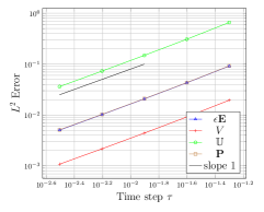
Figure 1. $L^{2}(\Omega)$ errors of each primal variables in the system (36) against the time step $\tau$. Note that the errors for ${\mathbf{E}}$ and ${\mathbf{P}}$ are so closed that their plots almost coincide.

Convergence in space

We next check the rate of convergence in space with an indirect approach. The idea is to guarantee that the error from the time discretization does not dominate the total error. To this end, we start to solve the discrete system under a uniform coarse mesh containing $16$ cells and setting the time step $\tau=T$. Then we refine the mesh globally and divide the time step by $2^{k+1}$, where we recall that $k=1$ or $2$ denotes the degree of bi-polynomials. So the time step $\tau=ch^{k+1}$ and according to the expected error bound (35), the total error should behave like $O(h^{k+1})$.

Figure 2 reports the $L^{2}(\Omega)$-error against the number of degrees of freedom (#DoFs) at $T=0.1$ using both bilinear and bi-quadratic elements. We observe that all $L^{2}(\Omega)$ errors for primal variables behave like $O(h^{k+1})$ since $h\sim\#\text{DoFs}^{-1/d}$.

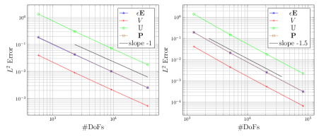
Figure 2. $L^{2}(\Omega)$ errors for each primal variable in the system (36) against #DoFs using continuous piecewise bilinear (left) and piecewise bi-quadratic elements (right), respectively. Note that similar to Figure 1, the errors for ${\mathbf{E}}$ and ${\mathbf{P}}$ are so closed that their plots almost coincide.

5.2. Monolayer tests

Now we test the numerical scheme (31) in a monolayer device which is $80nm$ long and $40nm$ wide. Figure 3 shows a uniform subdivision of the test device. In terms of the time discretization, we set the final time $T=160ns$ and the time step $\tau=T/1000$. For the parameters of the GLD model (2), we set $\epsilon_{b}=5F/m$, $\alpha=-1.54\times 10^{9}m/F$, $\beta=-2.65\times 10^{12}m^{5}/FC^{2}$, $\gamma=2.6\times 10^{15}m^{9}/FC^{4}$ and $g=10^{-8}m^{3}/F$.

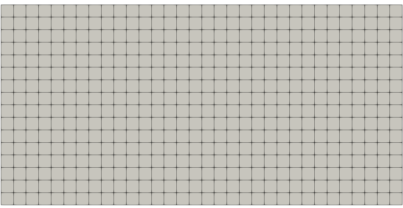
Figure 3. Subdivision of the monolayer test device.

5.2.1. Test for the energy stability

We first numerically check the energy stability of our proposed scheme. Here we set zero electric distribution in the device (i.e., $\rho=0$) and apply zero voltages at both the top and bottom. We also set the zero Neumann boundary conditions on both left and right boundaries of the device. That is $(\epsilon{\mathbf{E}}+{\mathbf{P}})\cdot\nu=0$ on $\{x_{1}=0\}\cup\{x_{1}=80nm\}$. Starting from the initial polarization field

$$P_{i}(t=0)=\left\{\begin{aligned} 0.1V/m,&\quad\text{ if }x_{1}\leq 40nm,\\ -0.1V/m,&\quad\text{ if }x_{1}\geq 40nm,\\ \end{aligned}\right.$$

we plot the approximation of the density of the total energy (7), i.e.,

$$d_{h}({\mathbf{P}}_{h}^{n}):=\frac{1}{|\Omega|}\int_{\Omega}\frac{\epsilon}{2}|\nabla V_{h}^{n}|^{2}+F({\mathbf{P}}_{h}^{n})+\sum_{i=1}^{2}\frac{1}{2g}|\mathbb{U}_{h}^{n}|^{2}\,\mbox{\rm d}x,$$

in the time range $[0,160ns]$ in Figure 4. In order to observe the decay of the energy density, we also plot $\text{sign}(d_{h})\log_{10}(d_{h})$ versus time in Figure 4 (noting that the minimum energy is negative). The approximation of the polarization field ${\mathbf{P}}_{h}$ at $80ns$ and $160ns$ as well as corresponding $\nabla\!\times\!{\mathbf{P}}_{h}$ are provided in Figure 5.

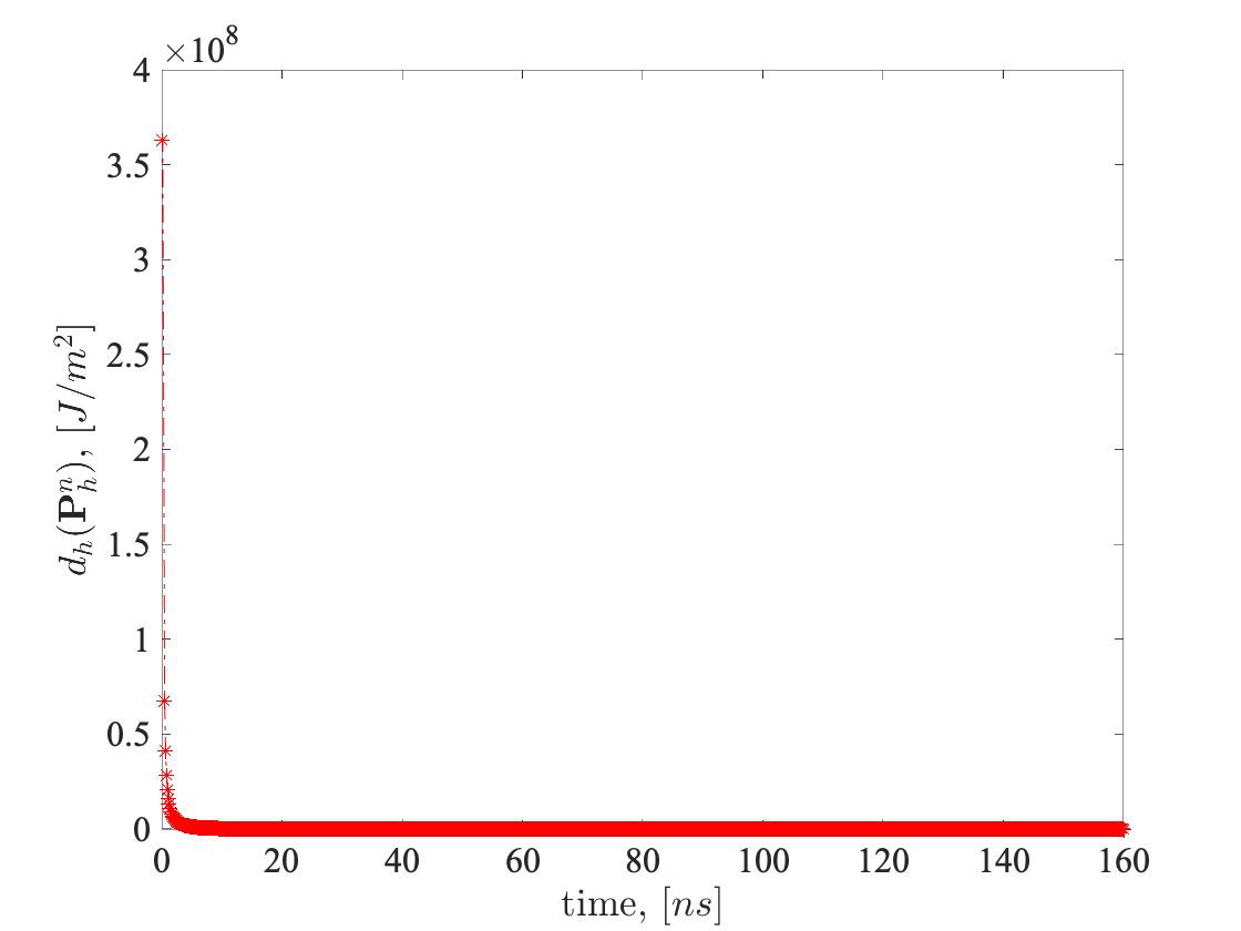
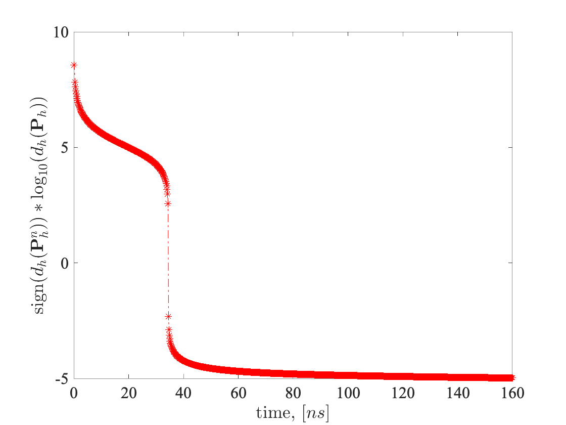
Figure 4. Test for the energy stability: decay of the energy (left) from $0ns$ and $160ns$ and its logarithm plot (right).

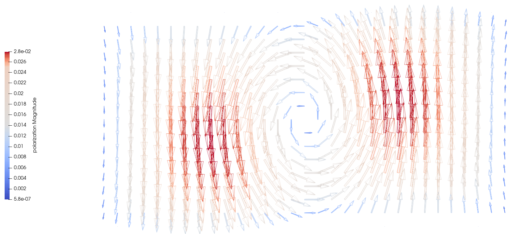
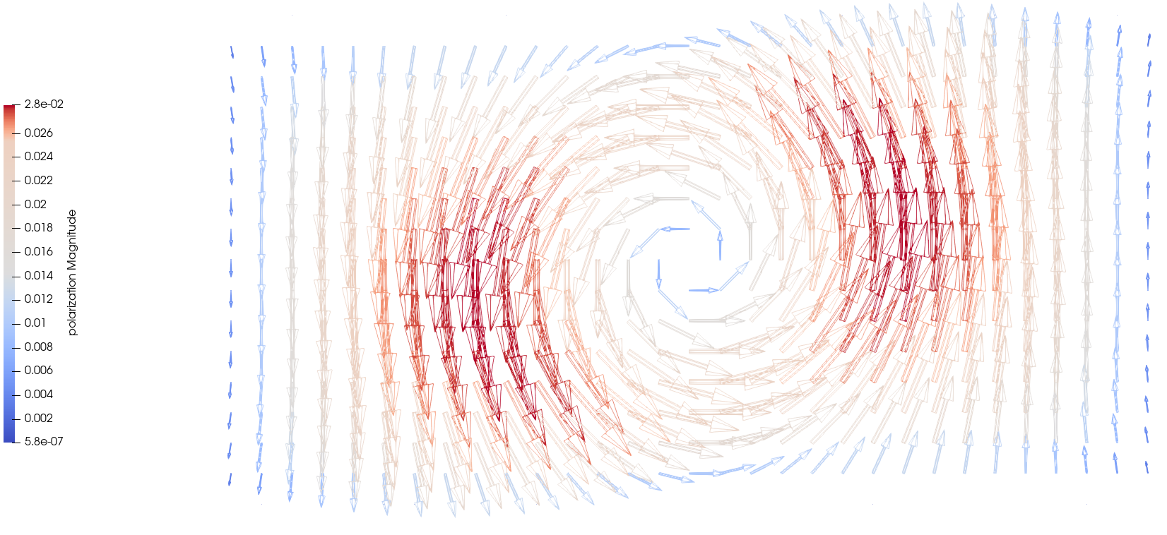
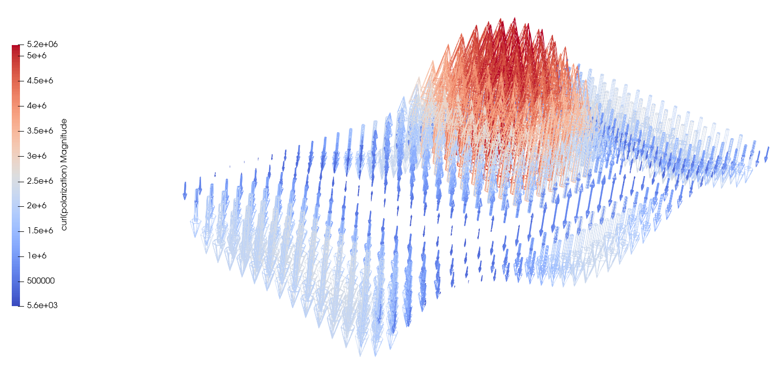
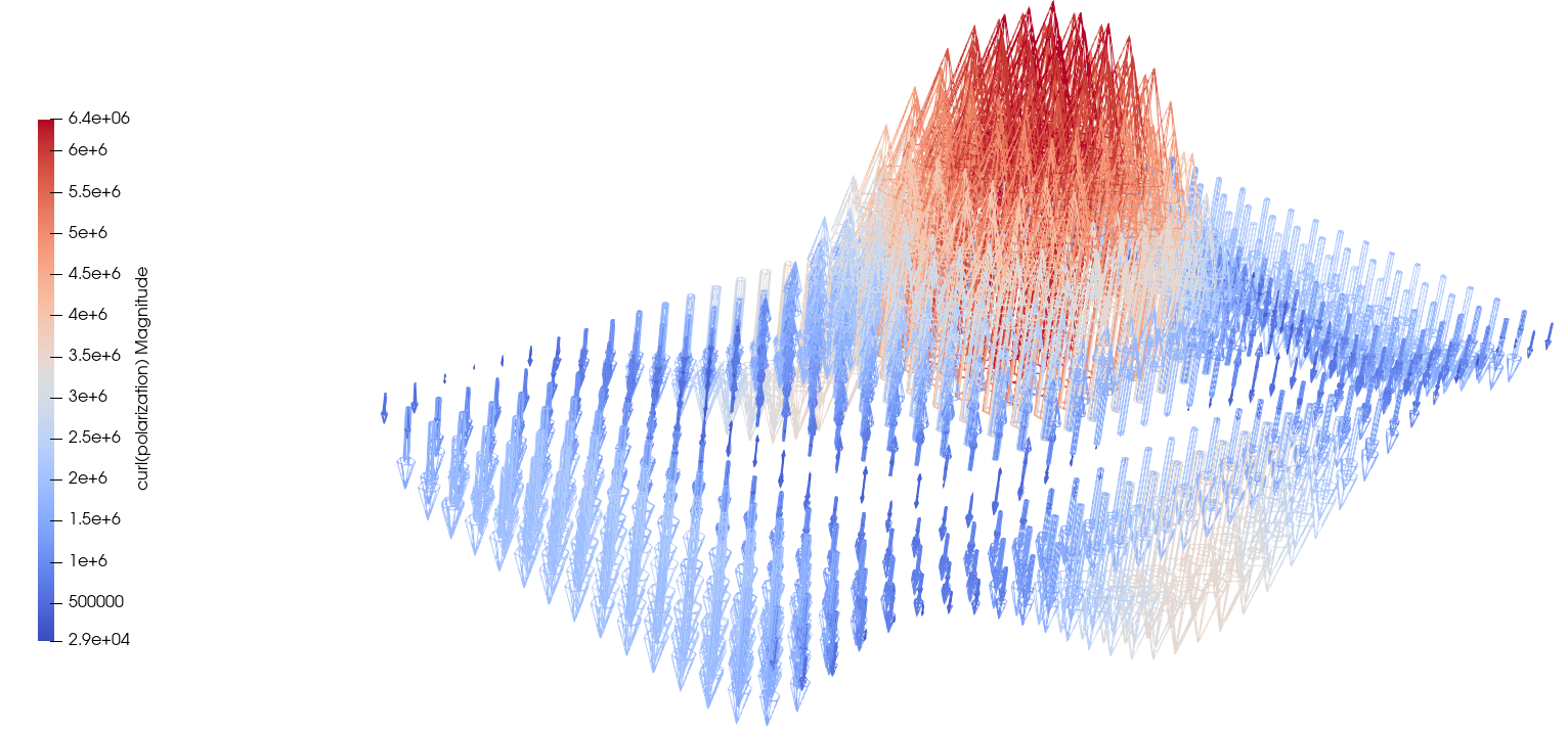
Figure 5. Test for the energy stability: approximations of the polarization field ${\mathbf{P}}_{h}$ at $80ns$ (top-right) and $160ns$ (top-right) as well as the plots for $\nabla\!\times\!{\mathbf{P}}_{h}$ at $80ns$ (bottom-right) and $160ns$ (bottom-right) . The magnitudes of ${\mathbf{P}}_{h}$ and $\nabla\!\times\!{\mathbf{P}}_{h}$ are rescaled by factors $3\times 10^{-7}$ and $4\times 10^{-15}$ respectively.

5.2.2. An integration test

Starting from the same discretization settings from the previous section, we fix the zero voltage at the bottom of the test device and apply different voltages on the top side with a contact bias following a triangle signal whose the first period is defined as

$$V(t)=\left\{\begin{aligned} 5t\,V,&\quad\text{ if }0\leq t\leq 20ns,\\ 200-5t\,V,&\quad\text{ if }20ns\leq t\leq 60ns,\\ -400+5t\,V,&\quad\text{ if }60ns\leq t\leq 80ns;\\ \end{aligned}\right.$$

see also the signal plot in Figure 6. In order to obtain accurate approximations, we locally refine the subdivision provided by Figure 3 every five time steps. More precisely speaking, after the computation at the time step $n=5k$ with $k=0,1,2,\ldots$, we estimate the error of the solution $V_{h}^{n}$ on each cell $K$ using the so-called Kelly error estimator [16]:

$$\eta_{K}^{2}=\sum_{F\in\partial K}\frac{\text{diam}(K)}{24}[\nabla V^{n}_{h}\cdot\nu]^{2}.$$

Then, we refine cells whose corresponding $\eta_{K}$ are 1% largest using the quad-refinement strategy (cf. [5]). The left plot of Figure 7 reports the discrete counterpart of the displacement vector

$$\int_{S}{\mathbf{D}}(t_{n})\cdot\nu\,\mbox{\rm d}s\approx\mathscr{D}:=\int_{S}(\epsilon\widehat{{\mathbf{E}}}^{n}_{h}+\widehat{\mathbf{P}}^{n}_{h})\cdot\nu\,\mbox{\rm d}s,$$

at top ($S=\{x_{2}=40ns\}$) and bottom ($S=\{x_{2}=0ns\}$) of the device against contact bias in one and a half periods (120ns in total). The right of Figure 7 shows the corresponding displacement current density $\int\partial_{t}{\mathbf{D}}\cdot\nu\,\mbox{\rm d}s$ versus time. Here we approximate this quantity by using the difference quotient $\,\mbox{\rm d}_{t,\tau}\mathscr{D}$. Both plots in Figure 7 shows that the polarization field switches its direction along $x_{2}$ direction. In order to show the dynamic of the polarization field, we report in Figure 8 the $x_{2}$-component of $\widehat{{\mathbf{P}}}^{n}_{h}$ along $x_{1}=40ns$ at $t=20j\,ns$ for $j=1,\ldots,5$. The corresponding background subdivisions are reported in Figure 8 as well. To illustrate the improvement of the accuracy from the adaptive refinement strategy, we plot $\widehat{V}^{n}_{h}$ along $x_{1}=40ns$ both on the meshes in Figure 5 and on the coarse mesh in Figure 3.

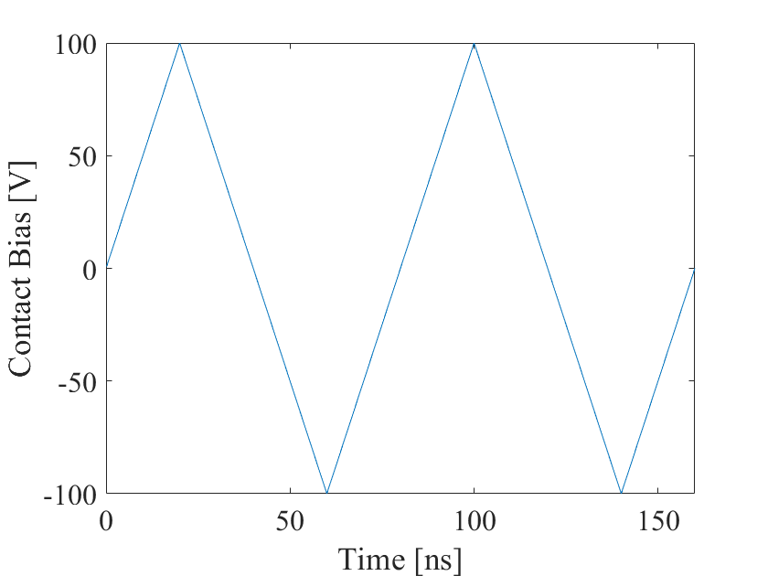
Figure 6. Signal of the contact bias in two periods.

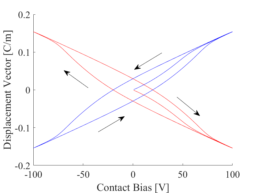
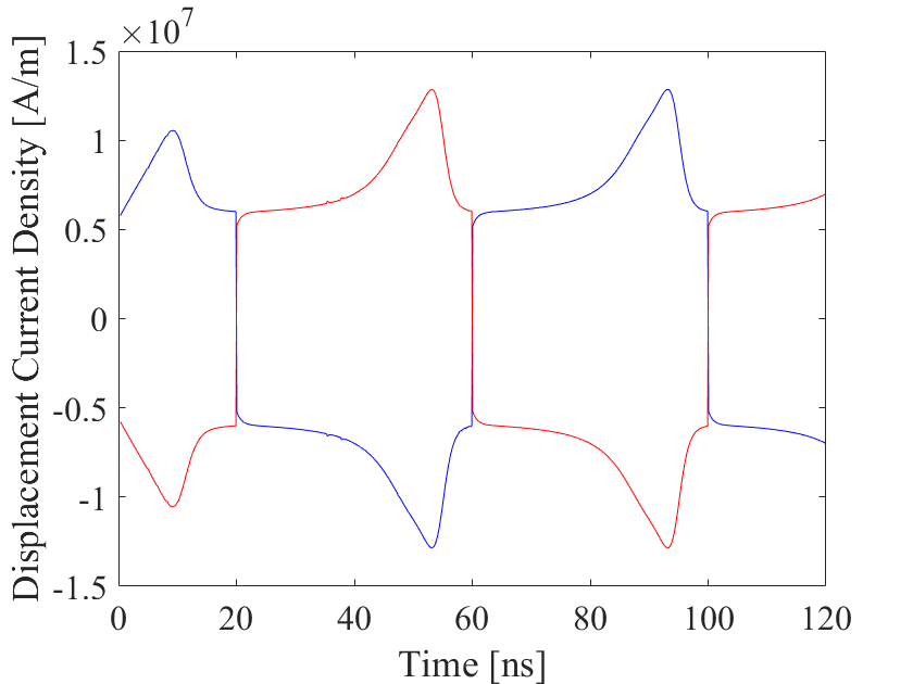
Figure 7. The left plot shows the displacement vector on top (in red) and bottom (in blue) versus the variation of the contact bias in $120ns$ (one and a half periods). The right plot shows the displacement current density against time.

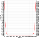
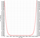
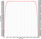
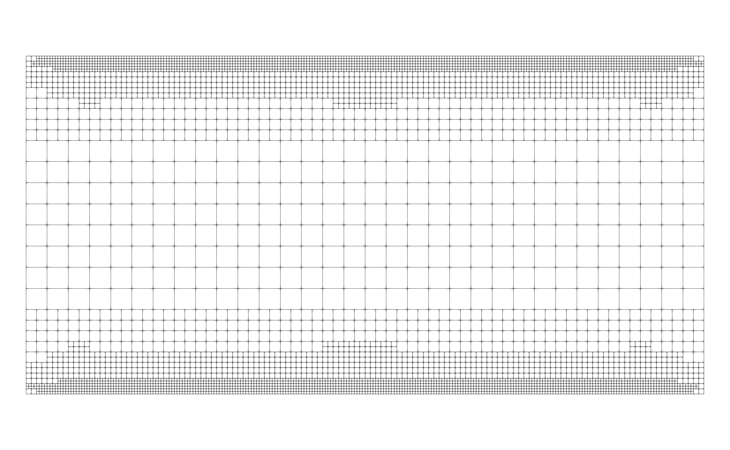
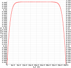
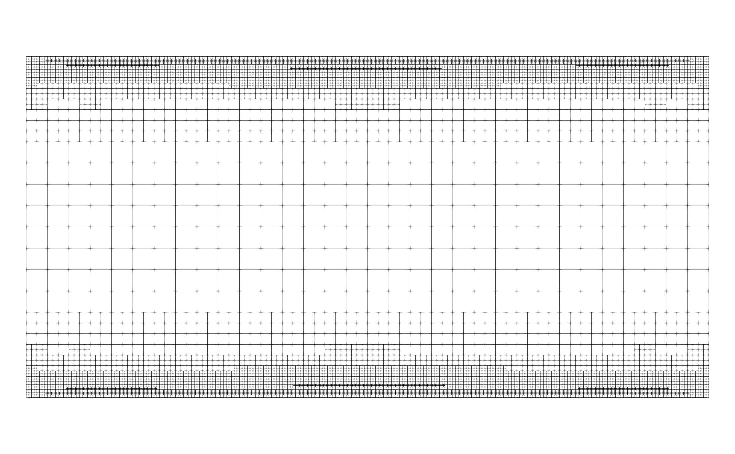
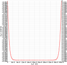
Figure 8. An integration test: (left column) the $x_{2}$ component of the approximated polarization field (i.e., $\widehat{{\mathbf{P}}}^{n}_{h}$) along $x_{1}=40ns$ at time $t=20j\,ns$ with $j=1,\ldots,5$ (from top to bottom) and (right column) the corresponding background subdivisions.

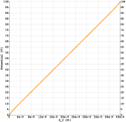
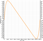
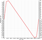
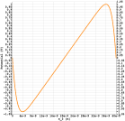
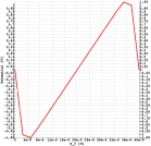
Figure 9. An integration test: the approximated potential (i.e., $\widehat{V}^{n}_{h}$) along $x_{1}=40ns$ at time $t=20j\,ns$ with $j=1,\ldots,5$ (from top to bottom) using the adaptive grids from Figure 5 (left column) and the corase grid from Figure 3 (right column).

6. Conclusion

We proposed a modified energy form $I({\mathbf{P}})$ based on Landau-Khalatnikov equation (6) and show that this energy form has at least one minimizer. We also show that the weak form of (6) admits at least one solution if the initial polarization field is in $[H^{1}(\Omega)\cap L^{\infty}(\Omega)]^{d}$ and charge distribution is in $H^{1}(0,T;L^{\infty}(\Omega))$. The solution is unique if the $L^{2}(\Omega)$-norm of $\Delta{\mathbf{P}}_{0}$ is finite. We designed an energy stable time-stepping scheme and we use an HDG scheme to discretize (6) in space. The numerical simulations verifies that the $L^{2}(\Omega)$-error for the primal variables converges in the rate $O(h^{k+1}+\tau)$, with $h$ and $\tau$ denoting the sizes in space grid and time grid, respectively. The future work includes the convergence analysis for the HDG scheme (31)–(33) as well as the analysis from the discrete solution to the minimizer of $I({\mathbf{P}})$.

There are no funders to report for this submission.

References

• [1] Günter Albinus, Herbert Gajewski, and Rolf Hünlich. Thermodynamic design of energy models of semiconductor devices. Nonlinearity, 15(2):367–383, February 2002.
• [2] Daniel Arndt, Wolfgang Bangerth, Bruno Blais, Thomas C. Clevenger, Marc Fehling, Alexander V. Grayver, Timo Heister, Luca Heltai, Martin Kronbichler, Matthias Maier, Peter Munch, Jean-Paul Pelteret, Reza Rastak, Ignacio Tomas, Bruno Turcksin, Zhuoran Wang, and David Wells. The deal.II library, version 9.2. Journal of Numerical Mathematics, 28(3):131–146, September 2020.
• [3] Sören Bartels. Numerical Methods for Nonlinear Partial Differential Equations. Springer International Publishing, 2015.
• [4] Sören Bartels, Rüdiger Müller, and Christoph Ortner. Robust a priori and a posteriori error analysis for the approximation of allen–cahn and ginzburg–landau equations past topological changes. SIAM journal on numerical analysis, 49(1):110–134, 2011.
• [5] Andrea Bonito and Ricardo H. Nochetto. Quasi-optimal convergence rate of an adaptive discontinuous Galerkin method. SIAM J. Numer. Anal., 48(2):734–771, 2010.
• [6] Philippe G Ciarlet. The finite element method for elliptic problems. SIAM, 2002.
• [7] Bernardo Cockburn, Jayadeep Gopalakrishnan, and Raytcho Lazarov. Unified hybridization of discontinuous galerkin, mixed, and continuous galerkin methods for second order elliptic problems. SIAM Journal on Numerical Analysis, 47(2):1319–1365, 2009.
• [8] Bernardo Cockburn, Jayadeep Gopalakrishnan, and Francisco-Javier Sayas. A projection-based error analysis of hdg methods. Mathematics of Computation, 79(271):1351–1367, 2010.
• [9] Albert Frederick Devonshire. Xcvi. theory of barium titanate: Part i. The London, Edinburgh, and Dublin Philosophical Magazine and Journal of Science, 40(309):1040–1063, 1949.
• [10] Xiaobing Feng and Andreas Prohl. Numerical analysis of the allen-cahn equation and approximation for mean curvature flows. Numerische Mathematik, 94(1):33–65, 2003.
• [11] Y. F. Gao and Z. Suo. Domain dynamics in a ferroelastic epilayer on a paraelastic substrate. J. Appl. Mech., 69(4):419–424, June 2002.
• [12] J. Hlinka and P. Márton. Phenomenological model of a $90^{\circ}$ domain wall inBaTiO3-type ferroelectrics. Physical Review B, 74(10), September 2006.
• [13] Michael Hoffmann, Milan Pešić, Stefan Slesazeck, Uwe Schroeder, and Thomas Mikolajick. On the stabilization of ferroelectric negative capacitance in nanoscale devices. Nanoscale, 10(23):10891–10899, 2018.
• [14] Hong-Liang Hu and Long-Qing Chen. Computer simulation of 90 ferroelectric domain formation in two-dimensions. Materials Science and Engineering: A, 238(1):182–191, 1997.
• [15] Tsutomu Ikegami, Koichi Fukuda, Junichi Hattori, Hidehiro Asai, and Hiroyuki Ota. A tcad device simulator for exotic materials and its application to a negative-capacitance fet. Journal of Computational Electronics, 18(2):534–542, 2019.
• [16] D. W. Kelly, J. P. De S. R. Gago, O. C. Zienkiewicz, and I. Babuska. A posteriori error analysis and adaptive processes in the finite element method: Part i—error analysis. International journal for numerical methods in engineering, 19(11):1593–1619, November 1983.
• [17] LD Landau and IM Khalatnikov. On the anomalous absorption of sound near a second order phase transition point. In Dokl. Akad. Nauk SSSR, page 25, 1954.
• [18] P. Lenarczyk and M. Luisier. Physical modeling of ferroelectric field-effect transistors in the negative capacitance regime. In 2016 International Conference on Simulation of Semiconductor Processes and Devices (SISPAD), pages 311–314. IEEE, September 2016.
• [19] Peter A. Markowich. The Stationary Semiconductor Device Equations. Springer Vienna, 1986.
• [20] Alexander Mielke. A gradient structure for reaction–diffusion systems and for energy-drift-diffusion systems. Nonlinearity, 24(4):1329, 2011.
• [21] Shinji Nambu and Djuniadi A Sagala. Domain formation and elastic long-range interaction in ferroelectric perovskites. Physical Review B, 50(9):5838, 1994.
• [22] Hyeon Woo Park, Jangho Roh, Yong Bin Lee, and Cheol Seong Hwang. Modeling of Negative Capacitance in Ferroelectric Thin Films. Advanced Materials, 31(32):1–23, 2019.
• [23] Oliver Penrose and Paul C Fife. Thermodynamically consistent models of phase-field type for the kinetic of phase transitions. Physica D: Nonlinear Phenomena, 43(1):44–62, 1990.
• [24] A. K. Saha, P. Sharma, I. Dabo, S. Datta, and S. K. Gupta. Ferroelectric transistor model based on self-consistent solution of 2d poisson's, non-equilibrium green's function and multi-domain landau khalatnikov equations. In 2017 IEEE International Electron Devices Meeting (IEDM), pages 13–5. IEEE, December 2017.
• [25] Sayeef Salahuddin and Supriyo Datta. Use of negative capacitance to provide voltage amplification for low power nanoscale devices. Nano letters, 8(2):405–410, December 2007.
• [26] Vidar Thomee. Galerkin finite element methods for parabolic problems. Springer Science & Business Media, 2007.