Exact-WKB analysis for SUSY and quantum deformed potentials:
Quantum mechanics with Grassmann fields and Wess-Zumino terms

Abstract

Quantum deformed potentials arise naturally in quantum mechanical systems of one bosonic coordinate coupled to $N_{f}$ Grassmann valued fermionic coordinates, or to a topological Wess-Zumino term. These systems decompose into sectors with a classical potential plus a quantum deformation. Using exact WKB, we derive exact quantization condition and its median resummation. The solution of median resummed form gives physical Borel-Ecalle resummed results, as we show explicitly in quantum deformed double- and triple- well potentials. Despite the fact that instantons have finite actions, for generic quantum deformation, they do not contribute to the energy spectrum at leading order in semi-classics. For certain quantized quantum deformations, where the alignment of levels to all order in perturbation theory occurs, instantons contribute to the spectrum. If deformation parameter is not properly quantized, their effect disappears, but higher order effects in semi-classics survive. In this sense, we classify saddle contributions as fading and robust. Finally, for quantum deformed triple-well potential, we demonstrate the P-NP relation, by computing period integrals and Mellin transform.

I Introduction and background

WKB method underwent a silent transformation, starting around 80s, turning it from an approximation with drawbacks concerning connection problem Berry ; Silverstone to a rigorous formalism for both mathematicians and physicists alike BPV ; Voros1983 ; Silverstone ; DDP2 ; DP1 ; Takei1 ; Takei2 ; Takei3 ; Kawai1 ; AKT1 ; Schafke1 ; Iwaki1 ; Alvarez3 ; Zinn-Justin:2004vcw ; Zinn-Justin:2004qzw ; Dunne:2013ada ; Dunne:2014bca . The new version, called exact WKB (sometimes called resurgent WKB) is an indispensable tool, not only in quantum mechanics, but also in diverse parts of theoretical physics and mathematics. The method has deep connections with 4d ${\cal N}=2$ gauge theories in the contexts of $\Omega$-deformation Nekrasov:2009rc ; Mironov:2009uv and wall-crossing phenomena Gaiotto:2012rg , as well as with ODE/IM correspondence Dorey:2001uw ; Dorey:2007zx , topological string theory, see e.g. Grassi:2014cla ; Grassi:2014zfa ; Kashani-Poor:2015pca ; Kashani-Poor:2016edc ; Ashok:2016yxz ; Ito:2018eon ; Hollands:2019wbr ; Ashok:2019gee ; Ito:2019jio ; Imaizumi:2020fxf ; Coman:2020qgf ; Allegretti:2020dyt ; Kuwagaki:2020pry ; Emery:2020qqu ; Enomoto:2020xlf ; Taya:2020dco ; Yan:2020kkb ; Duan:2018dvj . The common tread of all these different examples is the quantization of an underlying classical curve.

The exact WKB method is combination of two parts, topological and asymptotic analysis. The construction starts with the complexification of the coordinate space and then uses the classical energy conservation relation $p^{2}=2(E-V(x))$ to turn the $x\in\mathbb{C}$ plane into a Stokes graph. The exact quantization condition is determined by the topology of the Stokes graph, and remains invariant under variations of the parameters and energy, as long as one does not encounter a topology change in Stokes graph. The computational part of the problem starts with the determination of the WKB wavefunction, which is an asymptotic series, obtained recursively from the non-linear Riccati equation. From this asymptotic series, one can obtain the expressions for perturbative/non-perturbative cycles (Voros multipliers), which are also asymptotic. For a streamlined introduction, see Kawai1 , for explicit construction and calculation in a physical problem, see DDP2 ; Sueishi:2020rug ; Sueishi:2021xti . The calculations can become tedious, however, at the end of the day, they carry tremendous merit which justifies the hard work. The final result of the formalism captures all perturbative, non-perturbative phenomena for all energy levels, large-order/low order resurgence, low-order-low-order constructive form of the resurgence and fairly non-trivial aspects of the spectrum at once.

In our earlier works, we considered various quantum mechanical systems with classical polynomial and periodic potentials, constructed exact quantization conditions, and provided a dictionary between the Airy-type and degenerate Weber-type building blocks of Stokes graphs, which is important for explicit computations Sueishi:2020rug ; Sueishi:2021xti . In this work, we consider systems where potential is modified by an $O(\hbar)$ quantum deformation. These systems are not rare, and they are physically interesting. Consider quantum mechanics of systems with a bosonic field $x(\tau)$ and $N_{f}$ Grassmann valued field $\psi_{i}(\tau)$ (generalization of supersymmetric QM Witten:1982df ) , or the systems in which bosonic field $x(\tau)$ is coupled to Wess-Zumino term with a spin-$S$ coupling Stone:1988fu . Such generalization appeared in Balitsky:1985in ; Aoyama:2001ca ; Behtash:2015loa . For $N_{f}=2,3,\ldots$ and general half-integer and integer $S$, these are related to quasi-exactly solvable systems Turbiner:1987nw . In the first case, by diagonalizing fermion number, and in the second case, by diagonalizing spin coupling, we reach to a collection of graded Hamiltonians. For example, for supersymmetric theory, we end up with two Hamiltionians, in the fermion number zero and one sectors, and in $N_{f}$-flavor theory, a collection of $2^{N_{f}}$ Hamiltonians. One can think of each Hamiltonian in this decomposition in terms of a potential,

$$V(x,\hbar)=\underbrace{V_{0}(x)}_{\rm classical}+\underbrace{\hbar pV_{1}(x)}_{\rm quantum\;deformation}\equiv\frac{1}{2}W^{\prime}(x)^{2}+\frac{\hbar p}{2}W^{\prime\prime}(x),$$ (1)

where the first term $V_{0}(x)$ is classical and the second term $\hbar V_{1}(x)$ is quantum induced. The quantum potentials that arise from $N_{f}$-Grassmann field theories, $p$ takes values in a quantized discrete set. We will also analytically continue the coefficient $p$ into ${\mathbb{R}}$. There are many interesting phenomena that arise from this continuation. It is our goal to investigate this interesting class of quantum deformed potentials via exact-WKB method.

These systems provide useful prototypes to semi-classically calculable instanton analysis in QFTs with a bosonic and multiple fermionic fields in diverse dimensions, if instanton size moduli is kept under control in some way Unsal:2007vu ; Unsal:2007jx ; Shifman:2008ja ; Poppitz:2009uq ; Anber:2011de ; Poppitz:2012sw ; Misumi:2014raa ; Fujimori:2019skd ; Misumi:2019upg ; Fujimori:2020zka ; Dorigoni:2017smz ; Demulder:2016mja ; Schepers:2020ehn . In the asymptotically free theories such as 2d sigma models and 4d gauge theories, taking control of the instanton size moduli by circle compactification, twisted boundary conditions or Higgsing, the semi-classical analysis become similar to quantum mechanical systems. Furthermore, we now understand that there are compactification of QFTs with ’t Hooft fluxes to QM systems which preserve various anomalies and non-perturbative saddle points, see eg. Unsal:2020yeh . In these theories, integrating out fermions in a weak coupling calculable regime induces an $O(\hbar)$ deformation to classical action, similar to our quantum deformed system. As such, deeper understanding of the quantum deformed potentials via exact WKB should be useful more broadly.

From the exact WKB analysis, we construct exact quantization conditions at energies below the barrier. These remain invariant under DDP formula DDP2 ; DP1 , which is same as reality of resurgent transseries Aniceto:2013fka . Next, we point out that the median resummation of exact quantization condition is immensely useful to extract physical results. In the latter form, all resurgent cancellations takes place at the level of median resummation of the quantization condition. This idea is used by Pham et.al.DDP2 ; DP1 to show the reality of energy spectrum, but not to calculate the spectrum. We take their analysis one step beyond, and solve for the non-perturbative contributions, which are automatically in physical form, free of all ambiguities. This is one of the main technical achievements of our analysis.

The solutions of median resummed quantization condition reveals a number of nice and intriguing physical results. The systems we study have finite action instantons and bions Unsal:2007vu ; Unsal:2007jx ; Shifman:2008ja ; Poppitz:2009uq ; Anber:2011de ; Poppitz:2012sw ; Misumi:2014raa ; Fujimori:2019skd ; Misumi:2019upg ; Fujimori:2020zka . Despite that, for certain quantized deformation parameters, part of the spectrum does not receive any non-perturbative contribution at all and perturbation theory converges and captures all (e.g. algebraically solvable states in QES and SUSY systems). In certain cases, there is a convergent/divergent alternation in the perturbative spectrum of low lying states. If the deformation parameter is not properly quantized, instantons end up not contributing to energy levels at leading order in semi-classics $e^{-S_{\rm I}/\hbar}$, and leading non-perturbative contributions are due to bions $e^{-S_{\rm B}/\hbar}\sim e^{-2S_{\rm I}/\hbar}$ and they are robust. The emergence of the traditional low-order/high order resurgence relations and all orders resurgent cancellations via the DDP formula DDP2 ; DP1 is also captured by the formalism. More profoundly, we used asymptotic expansion of WKB wave functions, quantum integrals over perturbative and non-perturbative cycles, and Mellin transform to prove that perturbation theory around perturbative vacuum for generic level number $k$ and generic $p$ determines all perturbative and non-perturbative information around non-perturbative bion saddles. This generalize P-NP relation between perturbation theory and instanton sectors Alvarez1 ; Alvarez2 ; Alvarez3 ; Dunne:2013ada ; Dunne:2014bca ; Dunne:2016qix ; Gahramanov:2015yxk ; Raman:2020sgw , and perturbation theory and bion sectors Kozcaz:2016wvy ; Dunne:2016jsr to quantum deformed potentials. This is a constructive low-order/low-order relation between different saddles in the problem and a generalization of the P-NP relations for these systems. The exact WKB formalism is capable to address all these phenomena in a unified fashion.

II Goals and Structure of this paper

In this section, we clarify the goal and the structure of this paper. The goals of this paper includes

1. to analyze the quantum mechanical systems with quantum deformed double- and triple-well potentials to obtain exact quantization conditions, understand the resurgent structure, and drive the median-resumed (ambiguity-cancelled) physical quantities,

2. to show the striking fact that the instantons with real and finite actions do not contribute to the energy spectrum in some cases depending on the deformation parameter,

3. to obtain a perturbative/non-perturbative (P-NP) relation for the quantum deformed triple-well quantum mechanics.

Since the Hamiltonians we focus on originate in the quantum mechanics including both bosonic and fermionic degrees of freedom, the above goals have significant implications for many fields as long as quantum mechanics is involved in them. For example, once we obtain an exact quantization condition for a certain quantum mechanical system, we can derive an exact energy spectrum and an exact partition function. We will show that one can obtain the exact quantization condition of quantum-deformed double- and triple-well systems by the exact-WKB analysis. We note that the eaact quantization condition for the triple-well system will be derived for the first time. Although we do not perform the numerical calculation to confirm our results, we check that these results are consistent with those obtained in the literature.

Now, let us introduce the structure of this paper: In Sec.III, we consider QM with Grassmann field and QM with topological Wess-Zumino term and explain how these theories relate to QM with the quantum deformed $N$-tuple well potential. In Sec.IV, in order to solve the puzzling of the energy spectra described above and their $p$-dependence, we introduce the exact WKB analysis and obtain the quantization condition by the cycle (Voros multiplier) expression. In this paper, in particular, we consider the cases of double-well and triple-well potentials as examples. In Sec.V, we solve the quantization condition and investigate the structure of the energy spectra from the aspect of Borel resummability. We also derive the P-NP relation and describe the connection to the path integral expression. In Sec.VI, we consider the median resummation of the quantization condition through the perturbative-non-perturbative relationship, i.e. the DDP formula, and derive the asymptotic solution of energy spectra without imaginary ambiguities. The results provide the solution of the puzzling. Sec.VII is devoted to the conclusions and prospects.

III QM with multiple Grassmann fields vs. Wess-Zumino terms

We consider two types of quantum mechanical systems.

• A bosonic field $x(t)$ and $N_{f}$ Grassmann valued field.

• A bosonic field $x(t)$ coupled to topological spin-$S$ Wess-Zumino term.

For $N_{f}=1$ and Wess-Zumino with $S={\textstyle{\frac{1}{2}}}$ Stone:1988fu ; Altland:2006si , the systems we are considering is ${\cal N}=1$ supersymmetric quantum mechanics. For $N_{f}=2,3,\ldots$ and $S=1,\frac{3}{2},\ldots,$ they are related to quasi-exactly solvable systems Turbiner:1987nw . We construct equivalent physical systems by using these two descriptions, and map them to quantum modified potentials Behtash:2015loa .

III.1 QM with $N_{f}$-Grassmann field

The Euclidean action for the first formulation is given by Behtash:2015loa

$$S=\frac{1}{g}\int d\tau\Big{(}{\textstyle{\frac{1}{2}}}\dot{x}^{2}+{\textstyle{\frac{1}{2}}}(W^{\prime})^{2}+\bar{\psi}_{i}(\partial_{\tau}+W^{\prime\prime})\psi_{i}\Big{)}\qquad i=1,\ldots,N_{f}$$ (2)

Below, we follow Behtash:2015loa ; Aoyama:2001ca to turn this system into a collection of quantum deformed potentials. Let us consider either the thermal or graded partition functions:

$$Z(\beta)={\rm Tr}_{\cal H}e^{-\beta H},\qquad\qquad\tilde{Z}(L)\equiv {\rm Tr}_{\cal H}(-1)^{F}e^{-LH}.$$ (3)

For the thermal partition function in path integral formulation, one imposes anti-periodic boundary conditions for Grassmann valued fields. The insertion of $(-1)^{F}$ converts the anti-periodic boundary conditions to periodic boundary conditions, hence, for graded partition function, one needs to use periodic boundary conditions. The integrations over the fermions can be done exactly in these QM systems:

$$Z_{\mp}\equiv\int Dx\prod_{i=1}^{N_{f}}D\bar{\psi}_{i}D\psi_{i}\;e^{-\int d\tau\left({\textstyle{\frac{1}{2}}}\dot{x}^{2}+{\textstyle{\frac{1}{2}}}(W^{\prime})^{2}+\bar{\psi}_{i}(\partial_{\tau}+W^{\prime\prime})\psi_{i}\right)}$$ (4)

$$=\int Dx\;e^{-\int d\tau{\cal L}_{\rm bos}}\;\Big{[}{\rm det}_{\mp}(\partial_{\tau}+W^{\prime\prime})\Big{]}^{N_{f}}\,.$$ (5)

The fermionic determinant can be calculated exactly Gozzi:1983qxk , and for anti-periodic and periodic boundary conditions, it gives

$$[{\rm det}_{\mp}(\partial_{\tau}+W^{\prime\prime})]=\left\{\begin{array}[]{cc}\Big{[}2\cosh\Big({\textstyle{\frac{1}{2}}}\int W^{\prime\prime}d\tau\Big{missing})\Big{]}&\qquad{\rm apbc}\cr\cr\Big{[}2\sinh\Big{(}{\textstyle{\frac{1}{2}}}\int W^{\prime\prime}d\tau\Big{)}\Big{]}&\qquad{\rm pbc}\end{array}\right.$$ (9)

Therefore, we can express the thermal partition function in the following useful form:

$${Z}(\beta) =\int Dx\;e^{-\int d\tau{\cal L}_{\rm bos}}\;\left[2\cosh{\textstyle{\frac{1}{2}}}\int d\tau W^{\prime\prime}\right]^{N_{f}}$$ (10)

$$=\int Dx\;e^{-\int d\tau{\cal L}_{\rm bos}}\sum_{k=0}^{N_{f}}{N_{f}\choose k}\left[e^{\int d\tau\frac{W^{\prime\prime}}{2}}\right]^{k}\left[e^{-\int d\tau\frac{W^{\prime\prime}}{2}}\right]^{N_{f}-k}$$ (11)

$$=\sum_{k=0}^{N_{f}}{N_{f}\choose k}\int Dx\;e^{-\frac{1}{g}\int d\tau\left({\textstyle{\frac{1}{2}}}\dot{x}^{2}+{\textstyle{\frac{1}{2}}}(W^{\prime})^{2}+(2k-N_{f})g\frac{W^{\prime\prime}}{2}\right)}\equiv\sum_{k=0}^{N_{f}}{N_{f}\choose k}Z_{k}$$ (12)

and graded one as:

$$\widetilde{Z}(L)=\sum_{k=0}^{N_{f}}{N_{f}\choose k}(-1)^{N_{f}-k}Z_{k}$$ (13)

Here, $Z_{k}$ is the partition function for a bosonic system with quantum modified potentials

$$V(x)={\textstyle{\frac{1}{2}}}(W^{\prime})^{2}+(2k-N_{f})g\frac{W^{\prime\prime}}{2}$$ (14)

which involves the classical part $O(g^{0})$ and a quantum induced part $O(g^{1})$. The decomposition (12) implies that the Hamiltonian ${\hat{H}}$ and the Hilbert space ${\cal H}$ of the $N_{f}$ flavor theory split as:

$${\hat{H}} =\bigoplus_{k=0}^{N_{f}}{\rm deg}({\cal H}_{(N_{f},k)}){\hat{H}}_{(N_{f},k)},\qquad{\rm deg}({\cal H}_{(N_{f},k)})=\textstyle{{N_{f}\choose k}}$$ (15)

$${\cal H} =\bigoplus_{k=0}^{N_{f}}{\rm deg}({\cal H}_{(N_{f},k)}){\cal H}_{(N_{f},k)},$$ (16)

where ${\rm deg}({\cal H}_{(N_{f},k)})$ is the degeneracy of a given sector, and $k$ acquires an interpretation as fermion number. Under fermion number modulo two, these sectors exhibit an alternating Bose-Fermi structure, similar to supersymmetric theory Witten:1982df

$$(-1)^{F}{\cal H}_{(N_{f},k)}=(-1)^{k}{\cal H}_{(N_{f},k)}$$ (17)

III.2 QM with topological Wess-Zumino term

Let us now consider the following bosonic QM system coupled to WZ term following Stone:1988fu .

$$S=\int d\tau\frac{1}{g}\Big{(}{\textstyle{\frac{1}{2}}}\dot{x}^{2}+{\textstyle{\frac{1}{2}}}(W^{\prime})^{2}\Big{)}+\int d\tau\;W^{\prime\prime}\;S\cos\theta+iS\int d\tau\;(1-\cos\theta)\partial_{\tau}\phi$$ (18)

where the last term is topological Wess-Zumino term (also called Berry phase action), see Altland:2006si for an introduction. The partition function for this QM system is the one of quantum mechanical particle with spin-$S$ coupled to “magnetic field” $W^{\prime\prime}$:

$${Z}_{S}(\beta)=\int DxD(\cos\theta)D\phi\;e^{-\frac{1}{g}\int\big{(}{\textstyle{\frac{1}{2}}}\dot{x}^{2}+{\textstyle{\frac{1}{2}}}(W^{\prime})^{2}\big{)}+\int SW^{\prime\prime}\cos\theta+iS(1-\cos\theta)\partial_{\tau}\phi}\;.$$ (19)

Here, $\tau\in S^{1}_{\beta}$ parametrize the base space, and $(\theta,\phi)\in S^{2}$ are target space coordinates corresponding to path integral representation of spin.

The path integral over $\int D(\cos\theta)D\phi$ can be done exactly and provides a nice example of localization. Consider

$${I}_{S}(\beta)=\int D(\cos\theta)D\phi\;e^{\int SW^{\prime\prime}\cos\theta+iS(1-\cos\theta)\partial_{\tau}\phi}\;.$$ (20)

Decomposing $\phi(\tau)$ to periodic part and winding number valued in integers, we can write

$$\phi(\tau)=\underbrace{{\widetilde{\phi}}(\tau)}_{\rm periodic}+\frac{2\pi k}{\beta}\tau,\qquad k\in{\mathbb{Z}}$$ (21)

Therefore, the path integral (20) can be written as a sum over the winding sectors, and path integral over periodic fields:

$${I}_{S}(\beta)=\sum_{k\in{\mathbb{Z}}}\int D(\cos\theta)D\widetilde{\phi}\;e^{\int SW^{\prime\prime}\cos\theta+iS\int\widetilde{\phi}\;\partial_{\tau}(1-\cos\theta)+iS\int\frac{2\pi}{\beta}k(1-\cos\theta)}\;.$$ (22)

In the middle term, we used an integration by parts. Now, we can perform $D\widetilde{\phi}$ integration exactly. It gives a Dirac-delta constraint over the $\theta(\tau)$ field of the form $\delta(S\partial_{\tau}(1-\cos\theta))\propto\delta(\partial_{\tau}\cos\theta)$. This forces $\theta(\tau)=\theta_{0}$ to be time independent. Therefore, the path integration (20) reduces to an ordinary integration:

$${I}_{S}(\beta)=\sum_{k\in{\mathbb{Z}}}\int d(\cos\theta_{0})\;\;e^{S\cos\theta_{0}\int W^{\prime\prime}+i2\pi Sk(1-\cos\theta_{0})}\;.$$ (23)

Using Poisson resummation, we can convert the sum over winding number to something we momentarily identify as a spectral sum

$$\sum_{k\in{\mathbb{Z}}}e^{i2\pi Sk(1-\cos\theta_{0})}=\sum_{\widetilde{m}\in{\mathbb{Z}}}\delta(S(1-\cos\theta_{0})-\widetilde{m})$$ (24)

Therefore, (22) can be written as:

$${I}_{S}(\beta)=\sum_{\widetilde{m}\in{\mathbb{Z}}}\int d(\cos\theta_{0})\;\;e^{S\cos\theta_{0}\int W^{\prime\prime}}\delta(S(1-\cos\theta_{0})-\widetilde{m})\;.$$ (25)

Dirac delta function gives a non-vanishing contribution if and only if $\cos\theta_{0}=1-\frac{\widetilde{m}}{S}$. Since $|\cos\theta_{0}|\leq 1$, the number of $\widetilde{m}$ contributing to the sum is constrained and finite. In fact, there are only $(2S+1)$ terms with $0\leq\widetilde{m}\leq 2S$ contributing to the integral. Defining $m=\widetilde{m}-S$, we can write (25) as

$${I}_{S}(\beta)=\sum_{m=-S}^{+S}e^{m\int W^{\prime\prime}}\;.$$ (26)

and the partition function in the presence of the Wess-Zumino term takes the form:

$${Z}_{S}(\beta)=\sum_{m=-S}^{+S}\;\int Dx\;e^{-\frac{1}{g}\int\big{(}{\textstyle{\frac{1}{2}}}\dot{x}^{2}+{\textstyle{\frac{1}{2}}}(W^{\prime})^{2}+mgW^{\prime\prime}\big{)}}$$ (27)

Clearly, $S={\textstyle{\frac{1}{2}}}$ system is equivalent to $N_{f}=1$ theory Stone:1988fu , which is ${\cal N}=1$ supersymmetric quantum mechanics Witten:1982df . For $N_{f}=2$, we have a spin ${\textstyle{\frac{1}{2}}}\otimes{\textstyle{\frac{1}{2}}}=1\oplus 0$ particle, a spin-1, and a spin-0 particle, therefore, we need to consider $S=1$ and $S=0$ systems together. In general, the mapping between QM with $N_{f}$ Grassmann fields and QM with WZ terms is following.

$$\underbrace{{\textstyle{\frac{1}{2}}}\otimes\ldots\otimes{\textstyle{\frac{1}{2}}}}_{N_{f}}=\bigoplus_{S=S_{\rm min}}^{S_{\rm max}}{\rm mult}(S)\;S\,,$$ (28)

where

$$S_{\rm max}=\frac{N_{f}}{2},\qquad S_{\rm min}=\left\{\begin{array}[]{ll}0&N_{f}{\rm\;even}\,,\cr{\textstyle{\frac{1}{2}}}&N_{f}{\rm\;odd}\,,\cr\end{array}\right.$$ (31)

and the multiplicity of the spin-$S$ sub-sector is given by

$$S=\frac{N_{f}}{2}-k,\qquad{\rm mult}(S)=\left\{\begin{array}[]{ll}1&k=0\,,\cr{N_{f}\choose k}-{N_{f}\choose k-1}&1\leq k\leq\lfloor\frac{N_{f}}{2}\rfloor\,.\cr\end{array}\right.$$ (34)

The relation between the partition function graded according to fermion number and spin representations is given by

$$Z(\beta)\equiv\sum_{k=0}^{N_{f}}{\rm deg}({\cal H}_{k})Z_{k}=\sum_{S=S_{\rm min}}^{S_{\rm max}}{\rm mult}(S)Z_{S}\,.$$ (35)

Our main point is simple: The quantum mechanical systems with potential of the form

$$V(x,g)={\textstyle{\frac{1}{2}}}(W^{\prime}(x))^{2}+gmW^{\prime\prime}(x)$$ (36)

arise naturally by the integration over Grassmannian fields $\psi_{i}(\tau)$ or integrating the spin fields. The leading term is classical potential and sub-leading one is quantum deformation. Since quantum deformed potentials are fairly general, we generalize exact WKB analysis for systems with such potentials.

III.3 General remarks on SUSY, QES and in between

The quantum mechanical systems obtained above, either by coupling the system to Grassmann valued fields or to a Wess-Zumino term, decompose to systems with quantum deformed potentials given in (1). For certain discrete subsets of $p$, these systems are related to either ${\cal N}=1$ supersymmetric (SUSY) Witten:1982df or quasi-exactly solvable (QES) quantum mechanics Turbiner:1987nw ; Kozcaz:2016wvy .

Let us restrict our attention to a properly quantized $p$, to a potential of the form (1). The SUSY and QES has the common feature that a subset of states are solvable to all orders in perturbation theory (denoted as ${\cal H}_{0}$ in (37)), and a further subset of ${\cal H}_{0}$ is solvable algebraically. In these systems, the Hilbert space split up as

$${\cal H}=\underbrace{{\cal H}_{0}}_{\rm finite}\oplus\underbrace{{\cal H}_{1}}_{\rm infinite}$$ (37)

In general, ${\cal H}_{0}$ is composed of finitely many states (only one state in SUSY case and $2,3,\ldots,M$ states in QES where $M$ is determined by $p$), and ${\cal H}_{1}$ is composed of infinitely many states. Which states in ${\cal H}_{0}$ are algebraically solvable depends on a criterion explained below. The states in ${\cal H}_{1}$ are not solvable algebraically. All the states in ${\cal H}$ can be treated in the framework of WKB, and asymptotic series for WKB wave-functions can be obtained as explained in the next section.

The states in ${\cal H}_{0}$ may or may not be exactly solvable non-perturbatively. The well-known criterion in SUSY QM which determines whether supersymmetry is broken or not generalize to QES, and indicates whether a state is algebraically solvable or not. Let us recall briefly the standard description in SUSY and then, state how it generalize to QES systems.

Unbroken vs. broken SUSY = QES vs. Pseudo-QES: The ${\cal N}=1$ supersymmetric QM is described by the supersymmetry algebra

$$\{Q,Q^{\dagger}\}=2H,\qquad\{Q,Q\}=0,\qquad[Q,H]=0,$$ (38)

where $H$ is Hamiltonian and $Q$ is supercharge. A representation for supersymmetry generators is

$$Q=(ip+W^{\prime}(x))\psi_{-},\qquad Q^{\dagger}=(-ip+W^{\prime}(x))\psi_{+}.$$ (39)

Supersymmetry algebra implies that the spectrum of supersymmetric theory is positive semidefinite, Spec$(H)\geq 0$, and every $E>0$ state is Bose-Fermi paired. To all orders in perturbation theory, there exists an $E=0$ state. However, there may or may not exists an $E=0$ state non-perturbatively depending on the nature superpotential $W(x)$ Witten:1982df .

Now, assume $E=0$ state exists. Supersymmetry algebra and the saturation of lower bound imply $Q^{\dagger}|\Psi_{0}\rangle=Q|\Psi_{0}\rangle=0$. If ground state is of the form $|0\rangle\otimes|0\rangle_{F}$, the action of $Q$ is automatically zero because $\psi_{-}|0\rangle_{F}=0$ and the action of $Q^{\dagger}$ can be zero iff $(-ip+W^{\prime})\Psi_{0}=0$, which implies $\Psi_{0}(x)=e^{+\frac{1}{\hbar}W(x)}$. If ground state is of the form $|0\rangle\otimes|1\rangle_{F}$, then we find $\Psi_{0}(x)=e^{-\frac{1}{\hbar}W(x)}$.

For polynomial $W(x)$, there are three possibilities concerning $e^{\pm\frac{1}{\hbar}W(x)}$, which can be used to show if a supersymmetric ground state exists. Exactly the same possibilities will be crucial in QES as well in determination of exact algebraic solvability of low lying states. These are:

• If $W(x)\rightarrow+\infty$ as $|x|\rightarrow\infty$, then $e^{-W(x)/\hbar}$ is normalizable, $e^{+W(x)/\hbar}$ is not.

• If $W(x)\rightarrow-\infty$ as $|x|\rightarrow\infty$, then $e^{+W(x)/\hbar}$ is normalizable, $e^{-W(x)/\hbar}$ is not.

  Unbroken SUSY or QES: If at least one of the $e^{\pm W(x)/\hbar}\in L^{2}(\mathbb{R})$, SUSY is unbroken and for QES, a subset of states in ${\cal H}_{0}$ are algebraically solvable. These states can be written as $P_{i}(x)e^{-W(x)/\hbar},\;i=1,\ldots,M$ where $P_{i}(x)$ are polynomials.

• If $\lim_{x\rightarrow+\infty}W(x)=-\lim_{x\rightarrow-\infty}W(x)$, then neither one of the $e^{\pm W(x)/\hbar}$ is normalizable.

  Broken SUSY or pseudo-QES: If $e^{\pm W(x)/\hbar}\notin L^{2}(\mathbb{R})$, SUSY is broken and none of the states in ${\cal H}_{0}$ are exactly solvable. In both SUSY and QES, the states in ${\cal H}_{0}$ are solvable perturbatively, but these are not normalizable, and there is no non-perturbative algebraic solutions. This latter case is called pseudo-QES.

For polynomial $W(x)$, the leading large $|x|$ behaviour determines the nature of states in ${\cal H}_{0}$ and this is given by

$$W(x)=\left\{\begin{array}[]{ll}x^{2m}+\ldots,&|x|\rightarrow\infty,\qquad\rm unbroken\;SUSY\;or\;QES\\ x^{2m+1}+\ldots,&|x|\rightarrow\infty,\qquad\rm broken\;SUSY\;or\;pseudoQES\end{array}\right\}$$ (42)

Therefore, the double-well potential $W(x)\sim x^{3}+\ldots$ is an example of second category and triple-well potential $W(x)\sim x^{4}+\ldots$ is an example of first category.

There are a set of puzzling facts about these systems that the exact WKB analysis address successfully. In the unbroken SUSY or QES case, algebraically solvable states in ${\cal H}_{0}$ do not receive instanton $e^{-S_{\rm I}/\hbar}$ or bion $e^{-S_{\rm B}/\hbar}$ contribution to their energies, despite the fact that both instantons and bions are finite action configurations that are present in the theory. Yet, states in ${\cal H}_{1}$ receive either $e^{-S_{\rm I}/\hbar}$ and/or $e^{-S_{\rm B}/\hbar}$ type contributions. In the broken SUSY and pseudo-QES cases, the states in ${\cal H}_{0}$ do not receive instanton $e^{-S_{\rm I}/\hbar}$, but receive bion $e^{-S_{\rm B}/\hbar}$ contribution to their energies. We explain these phenomena in terms of destructive/constructive interference associated with the hidden topological angles Behtash:2015kna . Higher states living in ${\cal H}_{1}$ receive either $e^{-S_{\rm I}/\hbar}$ and/or $e^{-S_{\rm B}/\hbar}$ type contributions.

If $p$ is generic real number, than these system are not part of SUSY or QES descriptions, but they are continuously connected to them. There are no algebraically solvable states in the spectrum. In such cases, there is no instanton contribution anywhere in the spectrum and all NP contributions are due to bions. The solutions of the exact quantization conditions explains all these phenomena at once.

IV Exact-WKB analysis for quantum deformed potentials

As described in the previous section, quantum mechanical systems with extra Grassmann fields or WZ terms naturally decompose into potential problems in which the potential is a combination of classical and quantum induced terms, see (14) and (36). Since $\hbar$ and $g$ are formally on the same footing, we can view these systems as Schrödinger equation with a potential $V(x,\hbar)=V_{0}(x)+\hbar V_{1}(x)$:

$$\left[-\hbar^{2}\frac{\partial^{2}}{\partial x^{2}}+Q(x,\hbar)\right]\psi(x,\hbar)=0,$$ (43)

where $Q(x,\hbar)=\sum_{n=0}Q_{n}(x)\hbar^{n}$ now includes both the classical as well as a quantum induced terms in potential. $Q(x,\hbar)$ is given by

$$Q_{0}(x)=2(V_{0}(x)-E),\qquad Q_{1}(x)=2V_{1}(x),\qquad Q_{n\geq 2}(x)=0,$$ (44)

with the energy $E$. The fact that we only included $Q_{1}$ is motivated by the two physical applications described in §. III. Here, the factor $2$ comes from $\hbar^{2}/2$ in the first term as a convention. Note that for this application, we only need $\hbar Q_{1}$ as quantum deformation to exact-WKB analysis. In this section, we would like to describe exact-WKB analysis for such quantum deformed potentials. The below part for exact-WKB analysis is written based on Kawai1 ; Iwaki1 ; Sueishi:2021xti ; DDP2 ; Takei3 . See those Refs. for detail.

Consider the ansatz for the WKB-wave function:

$$\psi_{a}(x,\hbar)=\sigma(\hbar)\exp\left[\int^{x}_{a}dx^{\prime}\,S(x^{\prime},\hbar)\right],\qquad S(x,\hbar)=\sum_{n=-1}^{\infty}S_{n}(x)\hbar^{n},$$ (45)

Substituting to (43) gives the nonlinear Riccati equation, which can be mapped to a recursive equation for $S_{n}(x)$.

$$S(x,\hbar)^{2}+\frac{\partial S(x,\hbar)}{\partial x}=\hbar^{-2}Q(x)$$ (46)

$$\Rightarrow\quad \begin{cases}S_{-1}(x)=\pm\sqrt{Q_{0}(x)}&\\ 2S_{-1}(x)S_{j}(x)+\sum_{k,\ell=0}^{k+\ell=j-1}S_{k}(x)S_{\ell}(x)+\frac{dS_{j-1}(x)}{dx}=Q_{j+1}(x)&\mbox{for }\ j\geq 0\end{cases}.$$ (47)

The formal power series solution of the wave function can ultimately be obtained from the $S_{n}(x)$. $\sigma(\hbar)$ in Eq.(45) is a normalization factor, which is a function independent of $x$. Since the Schrödinger equation is an second order equation, it gives two independent solution associated with the sign in Eq.(47). Let us denote them $S^{(\pm)}(x,\hbar)=\sum_{n=-1}^{\infty}S^{(\pm)}_{n}(x)\hbar^{n}$ with $S^{(\pm)}_{-1}=\pm\sqrt{Q_{0}(x)}$. Define $S_{\rm odd/even}(x,\hbar)$ as the formal expansion with $S_{\rm odd/even}(x,\hbar)=\sum_{n=-1}^{\infty}S_{{\rm odd/even},n}(x)\hbar^{n}$ given by

$$S_{\rm odd}(x,\hbar):=\frac{S^{(+)}(x,\hbar)-S^{(-)}(x,\hbar)}{2},\qquad S_{\rm even}(x,\hbar):=\frac{S^{(+)}(x,\hbar)+S^{(-)}(x,\hbar)}{2}.$$ (48)

Note that odd/even is the name for the way linear combination is formed. It does not imply that $S_{\rm odd/even}(x,\hbar)$ has only odd/even powers of $\hbar$ when $Q_{n>0}(x)\neq 0$, unlike the case of classical potentials for which only $Q_{0}(x)\neq 0$. From Eq.(46), one can directly show that

$$S_{\rm even}(x,\hbar)=-\frac{1}{2}\frac{\partial\log S_{\rm odd}(x,\hbar)}{\partial x},$$ (49)

and thus, the formal wavefunction $\psi_{a}(x,\hbar)=(\psi^{+}_{a}(x,\hbar),\psi^{-}_{a}(x,\hbar))^{\top}$ is obtained as

$$\psi_{a}^{\pm}(x,\hbar)=\frac{\sigma_{\pm}(\hbar)}{\sqrt{S_{\rm odd}(x,\hbar)}}\exp\left[\pm\int^{x}_{a}dx^{\prime}\,S_{\rm odd}(x^{\prime},\hbar)\right].$$ (50)

The pre-factor $\sigma_{\pm}(\hbar)$ is chosen such that $\sigma_{\pm}(\hbar)=1$ when $a\in{\rm TP}$ where ${\rm TP}$ is a set of turning points determined by $Q_{0}(x)=0$. Note that the quantum deformation of the potential does not alter the Stokes graph or $S_{-1}(x)$ which are dictated by classical data, but it feeds into all the higher order terms in $S(x,\hbar)$, which is obtained by recursively solving (47).

Whether the WKB wave function is Borel summable or not is dictated by the classical data of the problem, namely the classical potential $V_{0}(x)$ or $S_{\rm odd,-1}(x)$. So it is helpful to draw the Stokes graph for classical potential, see Fig.1. Note that quantum deformation does not enter to the determination of the Stokes graph. When $E=E(\hbar):=\sum_{n=0}^{\infty}E_{n}\hbar^{n}$ with finite $E_{0}$ in the $\hbar\rightarrow 0$ limit, the graph defined by $V_{0}(x)=W^{\prime}(x)^{2}/2$ locally constitutes of the Airy-type Stokes graph. We define a set of turning points as

$${\rm TP}:=\{x\in{\mathbb{C}}\ |\ Q_{0}(x)=0\},$$ (51)

and the Stokes curve associated with $a\in{\rm TP}$ is defined as

$$\imaginary\frac{1}{\hbar}\int_{a}^{x}\sqrt{Q_{0}(x)}dx=0\,.$$ (52)

Clock-wise crossing a Stokes line emerging from a turning point $a$ can be expressed by $\psi_{{\rm I},a}(x,\hbar)=M_{\pm}\psi_{{\rm II},a}(x,\hbar)$, where

$$M_{+}=\begin{pmatrix}1&&i\\ 0&&1\end{pmatrix},\qquad M_{-}=\begin{pmatrix}1&&0\\ i&&1\end{pmatrix}.$$ (53)

Since the connection formula Eq.(53) is locally defined around each turning point, one must change a normalization point before crossing a line emerging from other turning points. This is carried out by $\psi_{a_{1}}(x,\hbar)=N_{a_{1},a_{2}}\psi_{a_{2}}(x,\hbar)$ with a normalization matrix $N_{a_{1},a_{2}}$, where

$$N_{a_{1},a_{2}}=\begin{pmatrix}e^{+\int_{a_{1}}^{a_{2}}dx\,S_{\rm odd}(x,\hbar)}&&0\\ 0&&e^{-\int_{a_{1}}^{a_{2}}dx\,S_{\rm odd}(x,\hbar)}\end{pmatrix},\qquad a_{1,2}\in{\rm TP}.$$ (54)

Additionally, branch-cuts also exist the Stokes graph. These cuts are nothing but exchange of $\psi^{+}_{a}(x,\hbar)$ with $\psi^{-}_{a}(x,\hbar)$, i.e. $+S_{\rm odd}(x,\hbar)$ with $-S_{\rm odd}(x,\hbar)$, hence, it can be realized by the branch-cut matrix $T$ given by

$$T=\begin{pmatrix}0&&-i\\ -i&&0\end{pmatrix}.$$ (55)

The quantization condition ${\mathfrak{D}}(E,\hbar)$ is obtained from the analytic continuation from $x=-\infty$ to $x=+\infty$ and the normalizability of the wavefunction. Starting with a WKB wavefunction that vanishes at $x=-\infty$, and using the rules of the passages through the Stokes lines, cuts, change of turning points as one proceeds to $x=+\infty$, one obtains a linear combination of the two WKB wavefunctions (50), an exponentially decaying and increasing wave function at $x=+\infty$. Demanding that wave function remains normalizable amounts to quantization condition. This amounts to setting the coefficient of the diverging WKB exponent at $x=+\infty$ to zero.

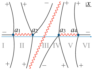
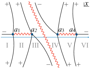
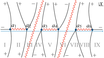
(a) Double-well (${\rm Im}\,\hbar>0$)    (b) Double-well (${\rm Im}\,\hbar<0$)

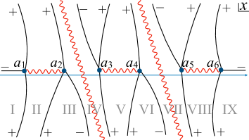
(c) Triple-well (${\rm Im}\,\hbar>0$)    (d) Triple-well (${\rm Im}\,\hbar<0$)

Figure 1: Stoke graphs for the double-well and triple-well potentials. We consider energy levels less than the top of the potential barrier, so all turning points are real. The blue points labeled by $a_{1},a_{2},\cdots$ are turning points, and the three Stokes lines, denoted by solid black lines, emerge from each of them. The red wave lines indicate branch-cuts, where the roles of $\psi^{+}$ and $\psi^{-}$ exchange. The quantization condition is computed going along the blue colored trajectory drawn slightly below the real axis from the left to the right as taking into account of the Stokes lines crossing the trajectory.

For ${\rm Arg}(\hbar)=0$, the WKB wave function is non-Borel summable since the theory is on a Stokes line. In order to go around this obstacle, (resolve the Borel nonsummability for the wavefunction), we introduce an infinitesimally small complex phase for $\hbar$ as $\hbar=|\hbar|e^{i\theta}$ with $0<|\theta|\ll 1$. Since the topology of the Stokes graph between positive and negative $\theta$ is different from each other, the difference in ${\mathfrak{D}}(E,\hbar)$ by the positive and negative $\theta$ corresponds to the source of the imaginary ambiguity cancellations.

For an $N$-tuple well potential with an energy $E$ less than any convexes of the potential, there are $2N$ real turning points. We denote them as $a_{1}<\cdots<a_{2N}\in{\rm TP}\subset{\mathbb{R}}$. Emanating from each turning point, there is a local Airy type building block, and Stokes graph can be viewed as a network of these building blocks as shown in Fig.1 for $N=2,3$. The symbols $\pm$ attached to the tip of each Stokes line denote the signs of asymptotic behavior of $S_{{\rm odd},-1}$ when taking the limit toward this direction for $x$. Since this graph is defined as the first Riemann sheet, $\psi_{+}(\psi_{-}$) is divergent when taking the limit to the region labeled by $+(-)$ but vanishes when reaching to $-(+)$. For the construction of the quantization condition ${\mathfrak{D}}$, we go along the blue line taken from $x=-\infty$ to $x=+\infty$ but slightly below the real axis as taking into account of monodromy matrices associated with each Stokes line $M_{\pm}$, normalization matrices $N_{a_{n_{1}},a_{n_{2}}}$, and branch-cut matrices $T$. For both $\imaginary(\hbar)=0^{\pm}$, there are $3N$ Stokes regions, where the WKB wave-functions are written as $\psi_{{\rm I},a_{1}}(x,\hbar),\ldots,\ldots,\psi_{{\rm 3N},a_{1}}(x,\hbar)$. The monodromy matrix of the $N$-tuple well potential connecting the WKB-wave functions can be expressed as

$$\psi_{{\rm I},a_{1}}(x,\hbar)={\cal M}\psi_{{\rm 3N},a_{1}}(x,\hbar),$$

$${\cal M}=\begin{cases}M_{+}N_{a_{1},a_{2}}\left[\prod_{n=1}^{N-1}M_{+}N_{a_{2n},a_{2n+1}}TM_{-}M_{+}N_{a_{2n+1},a_{2n+2}}\right]M_{+}N_{a_{2N},a_{1}}=:{\cal M}^{+}&\mbox{for $\theta>0$}\\ M_{+}N_{a_{1},a_{2}}\left[\prod_{n=1}^{N-1}M_{+}M_{-}N_{a_{2n},a_{2n+1}}TM_{+}N_{a_{2n+1},a_{2n+2}}\right]M_{+}N_{a_{2N},a_{1}}=:{\cal M}^{-}&\mbox{for $\theta<0$}\\ \end{cases}.$$

The Stokes graph for the double-well and triple-well potentials are shown in Fig.1. For example, the monodromy matrix for $N=2$ is obtained as

$${\cal M}^{+} = \begin{pmatrix}1+B^{-1}+A_{1}^{-1}B^{-1}&i(1+A_{1})(1+A_{2}^{-1})+iA_{1}A_{2}^{-1}B\\ -iA_{1}^{-1}B^{-1}&1+A_{2}^{-1}\end{pmatrix},$$ (57)

$${\cal M}^{-} = \begin{pmatrix}B^{-1}(1+A_{1}^{-1})&i(1+A_{1})(1+A_{2}^{-1})+iB\\ -iA_{1}^{-1}B^{-1}&1+A_{2}^{-1}+B\end{pmatrix},$$ (58)

where we defined $A$-(perturbative) and $B$-(non-perturbative) cycles in terms of all orders $S_{\rm odd}(x,E,\hbar)$, which dictates the WKB wave function:

$$A_{\ell}(E,\hbar)=\exp\left[\frac{1}{\hbar}\oint^{a_{2\ell}}_{a_{2\ell-1}}dx\,S_{\rm odd}(x,E,\hbar)\right],\qquad B_{\ell}(E,\hbar)=\exp\left[\frac{1}{\hbar}\oint^{a_{2\ell+1}}_{a_{2\ell}}dx\,S_{\rm odd}(x,E,\hbar)\right].$$ (59)

$A_{\ell}$ and $B_{\ell}$ give, respectively, oscillation in a locally bounded potential and tunneling effect between neighboring vacua, because $\oint^{a_{2\ell}}_{a_{2\ell-1}}dx\,S_{{\rm odd},-1}(x,E)\in i{\mathbb{R}}$ and $\oint^{a_{2\ell+1}}_{a_{2\ell}}dx\,S_{{\rm odd},-1}(x,E)\in{\mathbb{R}}_{<0}$. This monodromy matrix provides us the quantization condition by using the fact that normalizable WKB-wave function must vanish at infinity. Now, the upper and lower components of the wavefunction asymptotically behave $e^{-c/\hbar}$ and $e^{+c/\hbar}$ with a real positive $c$ at $|x|=\infty$, respectively, so that the normalizability of the analytically-continued function, $\psi_{{\rm I}a_{1}}$, requires the condition that the 1-2 component of ${\cal M}$ must be zero. Hence, one can determine the quantization condition as:

$$\lim_{|x|\rightarrow\infty}\psi_{{\rm I}_{a_{1}}}(x,|\hbar|e^{i0^{\pm}})=0\Longrightarrow\;\;{\mathfrak{D}}^{\pm}(E,\hbar):={\cal M}^{\pm}_{12}=0.$$ (60)

For $N=2,3$, ${\mathfrak{D}}^{\pm}(E,\hbar)$ is given by:

Double-well $$:$$

$${\mathfrak{D}}^{\pm}(E,\hbar) = \left(1+{A}_{1}\right)\left(1+{A}_{2}^{-1}\right)+\begin{cases}{A_{1}}{B}&\mbox{for $+$}\\ {A_{2}}^{-1}{B}&\mbox{for $-$}\end{cases},$$ (61)

Triple-well $$:$$

$${\mathfrak{D}}^{\pm}(E,\hbar) = (1+{A}_{1})(1+{A}_{2}^{-1})(1+{A}_{3})$$ (62)

$$+\begin{cases}{A}_{1}(1+{A}_{3}){B}_{1}+(1+{A_{1}}){A}_{3}{B}_{2}+{A}_{1}{A}_{3}{B}_{1}{B}_{2}&\quad\mbox{for $+$}\\ {A}_{2}^{-1}(1+{A}_{3}){B}_{1}+(1+{A}_{1}){A}_{2}^{-1}{B}_{2}+{A}_{2}^{-1}{B}_{1}{B}_{2}&\quad\mbox{for $-$}\end{cases}.$$

V Analysis via the quantization condition

In this section, we derive the quantization condition expressed by perturbative and non-perturbative cycles and consider energy spectra. We also derive a nontrivial relation, which is called P-NP relation, among a perturbative cycle, a nonperturbarive cycle, and energy for quantum deformed double and triple well potentials. This is an exact and constructive version of resurgence which relates perturbative expansion around the perturbative vacuum to the expansion around instanton or bion configurations. It is an early term/early term relation, unlike traditional resurgence which is late term/early term relation. For example, given the perturbative expansion of energy as a function of level number $N$ and coupling $g$ at some order $K$, we can derive the perturbative expansion around the instanton or bion at order $K-1$.

In this paper, we consider quantum deformed potentials $V(x,\hbar)=\frac{1}{2}W^{\prime}(x)^{2}\pm\frac{\hbar p}{2}W^{\prime\prime}(x)$ where

Double-well $$: \quad W^{\prime}(x)=x^{2}-\frac{1}{4},$$ (63)

Triple-well $$: \quad W^{\prime}(x)=\frac{1}{2}x(x^{2}-1),$$ (64)

$O(\hbar^{0})$ part in the potential is classical and $O(\hbar)$ part is quantum deformation. We also also argue the extension of our quantization conditions to generic superpotential $W(x)$.

V.1 Voros multipliers and quantization condition

The exact-WKB method is a combination of two parts, topological construction and analytic computation. The analysis that leads to exact quantization condition (60) is topological, and is dictated by the Stokes graph data. This is, however, half of the story. The important points provided by the exact-WKB analysis is that the quantization condition can be expressed by Voros multipliers or cycles. The analytic part of the story is the calculation of the Voros symbols by using all orders asymptotic expansion of (45). Since the Stokes automorphism can be simply written for each cycle DDP2 , the resurgence relation for objects derived from the quantization condition can be explicitly written. One can define two type of cycles, perturbative cycles ($A$-cycles) and non-perturbative cycles ($B$-cycles), given in (59). Roughly speaking, $A$-cycle express the perturbative fluctuations around a perturbative vacuum and $B$-cycle express the tunneling effect between two vacua including perturbative fluctuation around it. The practical side of the exact-WKB analysis involves explicit computation of these Voros symbols.

In §. IV, we have explained the exact-WKB method using the Airy-type, i.e., each of Stokes curve emerges from a simple turning point. Now, we introduce the degenerate Weber(DW)-type exact-WKB method. In this method, we firstly rescale the energy $E$ in the Schrödinger equation as $E\hbar$, and then draw the Stokes graph. This is just a redefinition of the variables, so it is physically equivalent to the Airy-type. But, since the definition of the Stokes curve is determined by the lowest order of $\hbar$ in the WKB expansion, it changes the condition giving the stokes curve as

$$\imaginary\frac{1}{\hbar}\int_{a}^{\infty}\sqrt{2(V_{0}-E)}dx=0\quad\to\quad\imaginary\frac{1}{\hbar}\int_{a}^{\infty}\sqrt{2V_{0}}dx=0,$$ (65)

where $a$ is a turning point. Also, if we set $E=O(\hbar)$ for a classical vacuum (minimum point), two simple turning points collide to each other and become a double turning point. Because of these differences, the monodromy matrix of the connection formula also changes significantly. (See (60) in Sueishi:2021xti .) Although computation of the DW-type is more complicated than that of the Airy-type, there are two reasons to introduce the DW-type method;

(I) The $\hbar$ expansion in the path integral calculation corresponds to the $\hbar$ expansion of the DW-type: In the path integral, the $\hbar$ expansion is performed by rescaling the quantum fluctuation as $x=x_{cl}+\sqrt{\hbar}\tilde{x}$ so that the gaussian part of $\tilde{x}$ is the zero-th order of $\hbar$ (regarding $\hbar$ expansion as coupling expansion), as follows:

$$Z =\int\mathcal{D}x\;e^{-\frac{S[x]}{\hbar}}=e^{-\frac{S[x_{cl}]}{\hbar}}\int\mathcal{D}\tilde{x}\;e^{-\tilde{x}M\tilde{x}+O(\sqrt{\hbar})}.$$ (66)

Let us consider this procedure from the viewpoint of Schrödinger equation. In the case of $V(x)=\displaystyle{\sum_{n=2}a_{n}x^{n}}$, the Schrödinger equation is expressed as

$$\quantity(-\frac{\hbar^{2}}{2}\frac{\partial^{2}}{\partial x^{2}}+a_{2}x^{2}+a_{3}x^{3}+...)\psi=E\psi.$$ (67)

In order to regard $\hbar$ as a coupling constant, we rescale $x=\sqrt{\hbar}\tilde{x}$ and $E=\tilde{E}\hbar$. Then, the Schrödinger equation becomes

$$\quantity(-\frac{1}{2}\frac{\partial^{2}}{\partial\tilde{x}^{2}}+a_{2}\tilde{x}^{2}+O(\sqrt{\hbar}))\psi=\tilde{E}\psi.$$ (68)

Notice that we rescaled not only $x$ but also $E$. This procedure should not change physics because it is just a redefinition of variables, but the difference arises when using exact-WKB to find the exact $\hbar$ asymptotic expansion of the partition function and energy. For example, terms related to $\log\hbar$ and the fluctuation determinant ($\det M$) cannot be naturally derived without using the DW-type.

(II) To obtain the hidden topological angle analytically: The hidden topological angle (HTA) is a phase produced by a quantum deformation part in the potential. As studied in Behtash:2015loa ; Behtash:2015kna ; Alireza2018 , this can also be interpreted as a phase associated with the action evaluated by a complex classical solution. In order to incorporate this contribution analytically in the form of Voros symbols, it is necessary to use the DW-type instead of the Airy-type. This is because even if the Voros symbol cannot be calculated analytically in the Airy-type, the DW-type can produce the HTA by factorization as $\mathfrak{A}=e^{ip\pi}\bar{\mathfrak{A}}$, where ${\mathfrak{A}}$ is a Voros symbol of the DW-type.

There is a precise dictionary connecting the Airy-type and the DW-type, and one needs to rewrite the exact quantization conditions (61) and (62) based on the Airy-type building blocks in terms of DW type building blocks. This amounts to

$${\rm Airy:}\;\;(A,B)\longrightarrow{\rm Degenerate\;Weber:}\;\;({\mathfrak{A}},{\mathfrak{B}})$$ (69)

and using the cycle expressions

$${\mathfrak{A}}_{\ell}(E,\hbar) = e^{2\pi iF_{\ell}(E,\hbar)},$$ (70)

$${\mathfrak{B}}_{\ell}(E,\hbar) = 2\pi{\mathfrak{B}}_{0}\prod_{\ell^{\prime}=0}^{1}\frac{C_{\ell+\ell^{\prime}-}(E,\hbar)}{C_{{\ell+\ell^{\prime}}+}(E,\hbar)}\frac{e^{(-1)^{\ell^{\prime}}\pi iF_{\ell+\ell^{\prime}}(E,\hbar)}\hbar^{F_{\ell+\ell^{\prime}}(E,\hbar)}}{\Gamma(1/2-F_{\ell+\ell^{\prime}}(E,\hbar))},$$ (71)

where ${\mathfrak{A}}_{\ell}$ and ${\mathfrak{B}}_{\ell}$ denote $A$-cycle and $B$-cycle, respectively, and $\ell$ is a label of each vacuum. In addition, ${\mathfrak{B}}_{0}$ the (classical) bion action, i.e. ${\mathfrak{B}}_{0}=e^{-S_{\rm B}/\hbar}$. Since a $B$-cycle attaches two $A$-cycles on the left and right sides, it includes the information of two $F_{\ell}(E,\hbar)$s. $F_{\ell}(E,\hbar)$ is easily calculable by performing residue integration around the $\ell$-th vacuum:

$$F_{\ell}(E,\hbar)=-{\rm Res}_{a=a_{\ell}}S_{\rm odd}(E,\hbar).$$ (72)

$C_{\ell\mp}(E,\hbar)$ in Eq.(71) can be obtained from the transformation connecting local and global coordinates Sueishi:2021xti . Calculation for the quantization condition using the DW-type requires reconstruction of the connection formula. However, without the explicit connection formula of the DW-type, we can easily perform the transformation of (69) by taking the following steps:

1. Find the Fredholm determinant $D$ in terms of the Voros symbols using the connection formula of Airy-type. (e.g. $D=1+A+AB$)

2. Replace the symbol via the Airy-Weber dictionary. (See Table I in Sueishi:2021xti ) (e.g. $D=1+\mathfrak{A}+\mathfrak{AB}$)

Therefore, using the results by the Airy-type, which are easy to calculate, we can produce the ones by DW-type. We emphasize that the DDP(Dellabaere-Dillinger-Pham) formula linking each Voros symbol with the Stokes phenomenon is also symbolically equivalent (e.g. $({\cal S}_{+}-{\cal S}_{-})[A]={\cal S}_{+}[AB]\to({\cal S}_{+}-{\cal S}_{-})[\mathfrak{A}]={\cal S}_{+}[\mathfrak{AB}]$), so that we can identify the resurgent structure directlySueishi:2021xti .

One of the nice properties of the quantum-deformed systems (1) is that in the asymptotic expansion of $\log{\mathfrak{A}}_{\ell}$ and $\log{\mathfrak{B}}$ in $\hbar$, the $O(\hbar^{0})$ term plays a special role, intimately related to hidden topological angle which is the phase of the bions as we describe later. It takes the form $\pi isp+({\rm energy})$ where $s\in\{-1,0,+1\}$ depending on a given potential. Thus, when $s=\pm 1$, it is convenient to split ${\mathfrak{A}}_{\ell}(E,\hbar)$ and/or ${\mathfrak{B}}_{\ell}(E,\hbar)$ into the phase factor and the other part for the later analysis:

$${\mathfrak{A}}_{\ell}(E,\hbar)=:e^{\pi isp}\bar{\mathfrak{A}}_{\ell}(E,\hbar),\qquad{\mathfrak{B}}_{\ell}(E,\hbar)=:e^{\pi isp}\bar{\mathfrak{B}}_{\ell}(E,\hbar),$$ (73)

where $\bar{\mathfrak{A}}_{\ell}(E,\hbar)$ and $\bar{\mathfrak{B}}(E,\hbar)$ are even functions of $p$. Similarly,

$$F_{\ell}(E,\hbar)=\frac{\log{\mathfrak{A}}_{\ell}}{2\pi i}=:\frac{sp}{2}+\bar{F}_{\ell}(E,\hbar),$$ (74)

where $F_{\ell}(E,\hbar)$ is given in (72). Here, $\bar{F}_{\ell}(E,\hbar)\equiv\sum_{n=0}^{\infty}\bar{F}_{\ell,n}\hbar^{n}$ is a formal power series dictated by WKB-wave function data $S(E,\hbar)$ (45), which is itself a formal series obtained by recursively solving Riccati equation (47).

For the double-well potential (63), the cycles (70) and (71) including only their leading order structure in $\hbar$ are given by:

$$\mbox{Double-well}:$$

$$\qquad{\mathfrak{A}}_{\ell}(E,\hbar)=e^{(-1)^{\ell}\pi ip}\bar{\mathfrak{A}}(E,\hbar)=e^{-2\pi i[E+(-1)^{\ell+1}p/2]}+O(\hbar),$$ (75)

$$\qquad{\mathfrak{B}}(E,\hbar)=\bar{\mathfrak{B}}(E,\hbar)=\frac{2\pi{\mathfrak{B}}_{0}}{\Gamma(E+\frac{1+p}{2})\Gamma(E+\frac{1-p}{2})}\left(\frac{\hbar}{2}\right)^{-2E}\left(1+O(\hbar)\right),$$ (76)

$$\qquad{\mathfrak{B}}_{0}=e^{-\frac{1}{3\hbar}},$$ (77)

Similarly, for the triple-well potential (64), the cycles take the form:

$$\mbox{Triple-well}:$$

$$\qquad{\mathfrak{A}}_{1,3}(E,\hbar)=e^{+\pi ip}\bar{\mathfrak{A}}(E,\hbar)=e^{-2\pi i(E-p/2)}+O(\hbar),$$ (78)

$$\qquad{\mathfrak{A}}_{2}(E,\hbar)=e^{-\pi ip}\bar{\mathfrak{A}}^{2}(E,\hbar)=e^{-2\pi i(2E+p/2)}+O(\hbar),$$ (79)

$$\qquad{\mathfrak{B}}_{\ell}(E,\hbar)=\bar{\mathfrak{B}}(E,\hbar)=\frac{2\pi{\mathfrak{B}}_{0}}{\Gamma(E+\frac{1-p}{2})\Gamma(2E+\frac{1+p}{2})}\cdot\frac{\hbar^{-3E}}{2^{E-\frac{p}{2}}}\left(1+O(\hbar)\right),$$ (80)

$$\qquad{\mathfrak{B}}_{0}=e^{-\frac{1}{4\hbar}},$$ (81)

Note that in the symmetric triple-well system (including its quantum deformation), the three $A$-cycles and two $B$-cycles can be expressed only by $\bar{\mathfrak{A}}(E,\hbar)$ and $\bar{\mathfrak{B}}(E,\hbar)$, respectively, meaning that it is in fact a genus-1 system, just like double-well potential. If one considers an asymmetric triple-well potential, it is no longer a genus-1 classical potential.

For the double-well and triple-well potentials and their quantum deformations, the quantization condition in terms of the DW-type cycles building blocks can be written as:

Double-well $$:$$

$${\mathfrak{D}}^{\pm} = \left(1+{\mathfrak{A}}_{1}\right)\left(1+{\mathfrak{A}}_{2}^{-1}\right)+\begin{cases}{\mathfrak{A}_{1}}{\mathfrak{B}}&\mbox{for $+$}\\ {\mathfrak{A}_{2}}^{-1}{\mathfrak{B}}&\mbox{for $-$}\end{cases}$$ (82)

$$= \left(1+e^{-\pi ip}\bar{\mathfrak{A}}\right)\left(1+e^{-\pi ip}\bar{\mathfrak{A}}^{-1}\right)+e^{-\pi ip}\bar{\mathfrak{A}}^{\pm 1}\bar{\mathfrak{B}},$$

Triple-well $$:$$

$${\mathfrak{D}}^{\pm} = (1+{\mathfrak{A}}_{1})(1+{\mathfrak{A}}_{2}^{-1})(1+{\mathfrak{A}}_{3})$$ (83)

$$+\begin{cases}{\mathfrak{A}}_{1}(1+{\mathfrak{A}}_{3}){\mathfrak{B}}_{1}+(1+{\mathfrak{A}_{1}}){\mathfrak{A}}_{3}{\mathfrak{B}}_{2}+{\mathfrak{A}}_{1}{\mathfrak{A}}_{3}{\mathfrak{B}}_{1}{\mathfrak{B}}_{2}&\quad\mbox{for $+$}\\ {\mathfrak{A}}_{2}^{-1}(1+{\mathfrak{A}}_{3}){\mathfrak{B}}_{1}+(1+{\mathfrak{A}}_{1}){\mathfrak{A}}_{2}^{-1}{\mathfrak{B}}_{2}+{\mathfrak{A}}_{2}^{-1}{\mathfrak{B}}_{1}{\mathfrak{B}}_{2}&\quad\mbox{for $-$}\end{cases}$$

$$= (1+e^{\pi ip}\bar{\mathfrak{A}})^{2}(1+e^{\pi ip}\bar{\mathfrak{A}}^{-2})$$

$$+\begin{cases}2e^{\pi ip}\bar{\mathfrak{A}}(1+e^{\pi ip}\bar{\mathfrak{A}})\bar{\mathfrak{B}}+e^{2\pi ip}\bar{\mathfrak{A}}^{2}\bar{\mathfrak{B}}^{2}&\qquad\mbox{for $+$}\\ 2e^{\pi ip}\bar{\mathfrak{A}}^{-2}(1+e^{\pi ip}\bar{\mathfrak{A}})\bar{\mathfrak{B}}+e^{\pi ip}\bar{\mathfrak{A}}^{-2}\bar{\mathfrak{B}}^{2}&\qquad\mbox{for $-$}\end{cases}$$

$$\propto \prod_{\varepsilon\in\{-1,+1\}}\left[(1+e^{\mp\pi ip}\bar{\mathfrak{A}}^{\mp 1})(1+i\varepsilon e^{\pm\pi i\frac{p}{2}}\bar{\mathfrak{A}}^{\mp 1})+\bar{\mathfrak{B}}\right],$$

where $\pm$ is the sign of the phase of complexified $\hbar=e^{i\theta}|\hbar|$, $\theta=0^{\pm}$.

These quantization conditions are invariant under the DDP formulaDP1 ; DDP2 :

$${\cal S}_{+}[\bar{\mathfrak{A}}]={\cal S}_{-}[\bar{\mathfrak{A}}](1+{\cal S}[\bar{\mathfrak{B}}])^{-1} \quad\Rightarrow\quad {\cal S}_{+}[{\mathfrak{D}}_{+}]={\cal S}_{-}[{\mathfrak{D}}_{-}].$$ (84)

which relates the left/right Borel resummation of the perturbative $A$-cycle to Borel resummation of the non-perturbative $B$-cycle. As a result, the Fredholm determinant remains invariant under Stokes automorphism, as $\arg(\hbar)$ moves from $0^{-}$ to $0^{+}$. This implies that all resurgent cancellations to all orders are already built-in the quantization condition.

We also should keep in our mind that the complex phase $e^{\pm ip\pi}$ attached to $\bar{\mathfrak{A}}(E,\hbar)$ is known as the Maslov index in the Gutzwiller trace formulaGutzwiller ; Alireza2018 ; Sueishi:2020rug and is related to a hidden topological angle in the path integral formalism, which will be discussed in Sec. V.5.

V.2 Nonpertubative effects in the energy spectrum, SUSY, QES, and in between

V.2.1 non-perturbative effect to the energy spectra

We now start to discuss the non-perturbative effect to the energy spectra of the quantum deformed theories, see Kozcaz:2016wvy ; Dunne:2016jsr ; Dunne:2020gtk ; Sato:2001ac for an earlier work from path integral perspective. One may naively be tempted to think that it is just the usual instanton analysis. However, the story is far more interesting, and captures many interesting non-perturbative phenomena. There are indeed some cases where instantons provide leading non-perturbative contributions, but also cases in which instantons do not contribute despite the fact that they are finite action solutions. There are also cases in which bions contribute at leading order, and other ones in which different bions have desctructive/constructive interference depending on hidden topological angle. When such destructive interference happens, perturbation theory is convergent, and the corresponding states turn out to be algebraically solvable. There is also a phenomenon called Cheshire cat resurgence taking place in these systems. When the quantum deformation parameter $p$ is analytically continued away from its quantized values, the convergence and destructive interference effects are replaced with the asymptotic nature of perturbative series and ambiguity of bion events which cancel each other out according to resurgence. In this sense, the non-perturbative phenomena we describe in these systems are quite rich.

The beauty of exact WKB is that all the interesting perturbative and non-perturbative phenomena can be extracted from the exact quantization condition obtained in Sec. V.1, at once, by replacing the cycles with their explicit forms. We will do this analysis in detail, starting with the simple aspects. The energy can be generally decomposed into two parts, that is a perturbative and a non-perturbative part. In order to obtain the energy spectrum, we first extract the perturbative part labeled the energy level denoted $k$ below, and then non-perturbative part by setting the boundary condition for the perturbative part with $\hbar\rightarrow 0_{+}$. The solution of exact quantization condition generates a transseries with all non-perturbative factors.

Let us demonstrate the process explicitly using the double-well and the triple-well potential. Let us first demonstrate how the simple harmonic energy levels emerge in the quantum-deformed double and triple well potentials. The quantization condition are given by Eqs.(82) and (83). Replacing $\bar{\mathfrak{A}}(E,\hbar)$ with the explicit form (75) and (78), and ignoring the non-perturbative contribution at first, we find:

Double-well $$: \qquad\left(1+e^{2\pi i(-E-p/2)}\right)\left(1+e^{2\pi i(E-p/2)}\right)=0,$$ (85)

Triple-well $$: \qquad\left(1+e^{-2\pi i(E-p/2)}\right)^{2}\left(1+e^{2\pi i(2E+p/2)}\right)=0.$$ (86)

Here, we picked up only the dominant parts in terms of $\hbar$. This provides harmonic energy spectrum for the quantum deformed potential.

Double-well $$: \qquad E_{\rm pt}=k+\frac{1\mp p}{2},$$ (87)

Triple-well $$: \qquad E_{\rm pt}=\begin{cases}\frac{1}{2}\left(k+\frac{1-p}{2}\right)&\mbox{for the inner-vacuum}\\ k+\frac{1+p}{2}&\mbox{for the outer-vacua}\end{cases},$$ (88)

with $k\in{\mathbb{N}}_{0}$ is the harmonic level number. $p=\pm 1$ correspond to supersymmetric pairs, with one zero energy level, and exhibiting the degeneracy (at the harmonic level) for higher states. For double-well, natural frequency is $\omega=1$ and for triple-well, it is $\omega_{\rm in}=1/2,\omega_{\rm out}=1$.

To obtain the leading non-perturbative contribution, we add $\delta(\hbar)$ to the energy as $E(\hbar)=E_{\rm pt}+\delta(\hbar)$, and keep non-perturbative term. Substituting $E(\hbar)$ into Eqs.(82) and (83) gives

$$\mbox{Double-well}:$$

$$\quad 4\sin(\pi\delta(\hbar))\sin[\pi(\delta(\hbar)-p)]$$

$$\quad\quad-\frac{2\pi{\mathfrak{B}}_{0}e^{\pm\pi i(p-2\delta(\hbar))}}{\Gamma(1+k+\delta(\hbar))\Gamma(1+k-p+\delta(\hbar))}\left(\frac{\hbar}{2}\right)^{-(1+2k-p+2\delta(\hbar))}=0,$$ (89)

$$\mbox{Triple-well (inner-vacuum)}:$$

$$\quad 4\cos\left[\pi\left(\frac{k}{2}+\frac{1-3p}{4}+\delta(\hbar)\right)\right]\cos\left[\pi\left(\frac{k}{2}+\frac{1+\varepsilon}{4}+\delta(\hbar)\right)\right]$$

$$\quad\quad+(-1)^{k}\frac{2\pi{\mathfrak{B}}_{0}e^{\mp\pi i\left(\frac{1}{2}-\frac{3p-\varepsilon}{4}+2\delta(\hbar)\right)}2^{-\left(\frac{1}{4}+\frac{k}{2}-\frac{3p}{4}+\delta(\hbar)\right)}\hbar^{-3\left(\frac{1}{4}+\frac{k}{2}-\frac{p}{4}+\delta(\hbar)\right)}}{\Gamma(\frac{3}{4}+\frac{k}{2}-\frac{3p}{4}+\delta(\hbar))\Gamma(1+k+2\delta(\hbar))}=0,$$

(90)

$$\mbox{Triple-well (outer-vacua)}:$$

$$\quad 4\sin\left[\pi\delta(\hbar)\right]\sin\left[\pi\left(\frac{3p+\varepsilon}{4}+\delta(\hbar)\right)\right]$$

$$\quad\quad-\frac{2\pi{\mathfrak{B}}_{0}e^{\mp\pi i\left(\frac{3p+\varepsilon}{4}+2\delta(\hbar)\right)}2^{-\left(\frac{1}{2}+k+\delta(\hbar)\right)}\hbar^{-3\left(\frac{1}{2}+k+\frac{p}{2}+\delta(\hbar)\right)}}{\Gamma(1+k+\delta(\hbar))\Gamma(\frac{3}{2}+2k+\frac{3p}{2}+2\delta(\hbar))}=0,$$ (91)

where $\varepsilon\in\{-1,+1\}$ and we used $E_{\rm pt}=k+\frac{1-p}{2}$ for the double-well potential without the loss of generality. By setting the boundary condition $\lim_{\hbar\rightarrow 0_{+}}\delta(\hbar)=0$, the solutions are obtained as

Double-well $$:$$

$$\delta_{p\in{\mathbb{Z}}}(\hbar) = {\cal P}\sqrt{\frac{{\mathfrak{B}}_{0}}{\pi\hbar\Gamma(1+k)\Gamma(1+k-p)}}\left(\frac{\hbar}{2}\right)^{-k+\frac{p}{2}}$$ (92)

$$-\frac{{\mathfrak{B}}_{0}}{\pi\hbar\Gamma(1+k)\Gamma(1+k-p)}\left(\frac{\hbar}{2}\right)^{-2k+p}\Phi_{\pm 1}(k,p)+O({\mathfrak{B}}_{0}^{3/2}),$$

$$\delta_{p\notin{\mathbb{Z}}}(\hbar) = (-1)^{1+k}\frac{{\mathfrak{B}}_{0}e^{\pm\pi ip}\Gamma(-k+p)}{\pi\hbar\Gamma(1+k)}\left(\frac{\hbar}{2}\right)^{-2k+p}$$ (93)

$$-\frac{2{\mathfrak{B}}_{0}^{2}e^{\pm 2\pi ip}\Gamma(-k+p)^{2}}{\pi^{2}\hbar^{2}\Gamma(1+k)^{2}}\left(\frac{\hbar}{2}\right)^{-4k+2p}\Phi_{\pm 1}(k,p)+O({\mathfrak{B}}_{0}^{3}),$$

where ${\cal P}\in\{-1,+1\}$ is the parity, and

$$\Phi_{n}(k,p):=\frac{\psi^{(0)}(1+k)+\psi^{(0)}(1+k-p)}{2}+\log\frac{\hbar}{2}+\pi ni,$$ (94)

with the polygamma function $\psi^{(n)}(x)$. Probably, the most striking feature of the solution (92) and (93) is that the instanton may or may not be the leading non-perturbative contribution depending on details. In fact, in generic case where $p$ is not quantized, the instanton contribution does not appear at all. Multiple remarks about this result are in order:

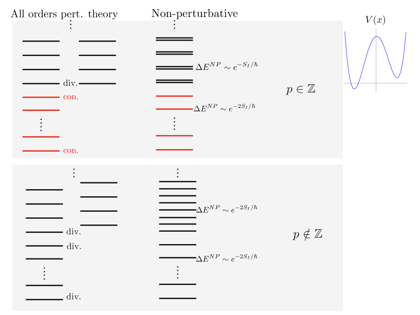
Figure 2: Perturbative vs non-perturbative spectrum of the quantum deformed double-well potential. For $p\in\mathbb{Z}$ (upper), lowest $p$ states have convergent , and higher ones have divergent perturbation theory. Non-perturbatively, the shift of the lowest $p$ states are of order $e^{-2S_{\rm I}/\hbar}$, and level splitting for higher states is $e^{-S_{\rm I}/\hbar}$. For $p\notin\mathbb{Z}$ (lower), all states have divergent perturbation theory. All perturbative energy levels are non-perturbatively shifted (up or down, depending on level number and $p$) by $e^{-2S_{\rm I}/\hbar}$ factor. Order $e^{-S_{\rm I}/\hbar}$ effects disappear from the spectrum.

• For the $p\in{\mathbb{Z}}$ case, consider the term proportional to instanton factor, $\sqrt{{\mathfrak{B}}_{0}}\sim e^{-S_{\rm I}/\hbar}$ in (92). This term is proportional to $\frac{1}{\Gamma(1+k-p)}$. Therefor, for level number $k=0,1,\ldots,p-1$, the argument of the gamma function is a negative integer, which corresponds to a pole of $\Gamma(x)$. As such, the instanton contribution vanishes for these states. The leading non-perturbative contribution arises from the bions for the lowest $p$ states. For $p=0$ (textbook case), of course, instanton contribution is present and it leads to level splitting between parity even and odd states. Note that for unquantized $p$ (93), there is no contribution to the spectrum at the one-instanton level, despite the fact that instantons are solutions of classical equations. This comes from the fact that harmonic states are not aligned for unquantized $p$.

• Since $\frac{\psi^{(0)}(z)}{\Gamma(z)}$ is an entire function, there is a non-perturbative contribution that arise from $\frac{\psi^{(0)}(1+k-p)}{\Gamma(1+k-p)}$ factor even when $k=0,1,2,p-1.$ In particular, the ambiguity of the bion contribution vanishes in these cases. Relatedly, perturbation series is convergent for these levels. However, for double-well in contrast with triple well, these levels are not exactly solvable mainly because $e^{\pm W(x)}$ are non-normalizable, while $e^{-W(x)}$ is normalizable for the triple-well.

• The bion contribution to the level $k$ of the $p$ deformed theory is of the form:

  $$\Delta E_{p,k}=-\frac{1}{2\pi\Gamma(1+k)}\left(\frac{\hbar}{2}\right)^{p-2k-1}\Gamma(p-k)e^{i\pi(p-k)}e^{-S_{\rm B}/\hbar}$$ (95)

  For supersymmetric theory, $p=1,k=0$ and the contribution is positive consistent with supersymmetry algebra. Note that the contribution of this bion to ground state ($k=0$) alternate as a function of $p$, increases the ground state energy for $p$ odd, and decreases it for $p$ even. For fixed $p$, bion contribution to higher states also alternates as a function of level number $k$. These two types of alternation in sign and the phase of the bion event is a consequence of what is called hidden topological angle. It also arise from the phase associated with Lefschetz thimble in path integral realization of this problem.

• For quantized $p$, states with level number $k\geq p-1$ on the lower harmonic well have degenerate pairs on the other well, and the degeneracy holds to all orders in perturbation theory. There is both instanton and bion contribution to the energy levels, leading to level splitting and shifting of the center-of-energy for the given level.

• For generic unquantized values of $p$, since there is no alignment of levels between the two wells, instanton contribution completely disappear for any level number $k$. The leading non-perturbative effects are due to bions as it arises naturally from exact-WKB (93).

These non-trivial features are consistent with supersymmetry and quasi-exact solvability structure in special cases. To convince ourselves, we can also compare the results with the calculations given in the literature. It is indeed in agreement with the results obtained by using a combination of path integral and Bender-Wu method for these problems Kozcaz:2016wvy . This does not yet complete our discussion of the quantum-deformed double-well potential. We will also determine order by order perturbation theory by using WKB-wave function, and verify explicitly P-NP relation between perturbation theory between perturbative and non-perturbative saddles.

For the triple-well, we set $p=(2q+1)/3$. The non-perturbative contribution is obtained as

$$\mbox{Triple-well}\ \mbox{(inner-vacuum)}:$$

$$\qquad\delta^{\varepsilon=(-1)^{q}}_{k+q\in 2{\mathbb{Z}}+1}(\hbar)=\mp i\frac{{\mathfrak{B}}_{0}2^{-\frac{1}{2}(2+k-q)}\hbar^{-\frac{1}{2}(1+3k-q)}}{\Gamma(1+k)\Gamma(\frac{1}{2}+\frac{k}{2}-\frac{q}{2})}$$

$$\qquad\qquad\qquad\qquad\quad+\frac{{\mathfrak{B}}_{0}^{2}2^{-(2+k-q)}\hbar^{-(1+3k-q)}}{\Gamma(1+k)^{2}\Gamma(\frac{1}{2}+\frac{k}{2}-\frac{q}{2})^{2}}\Psi^{(1)}_{\pm 2}\left(k,\frac{2q+1}{3}\right)+O({\mathfrak{B}}_{0}^{3}),$$ (96)

$$\qquad\delta^{\varepsilon=(-1)^{q+1}}_{k+q\in 2{\mathbb{Z}}+1}(\hbar)={\cal P}\sqrt{\frac{{\mathfrak{B}}_{0}}{\pi\Gamma(1+k)\Gamma(\frac{1}{2}+\frac{k}{2}-\frac{q}{2})}}2^{-\frac{1}{4}(2+k-q)}\hbar^{-\frac{1}{4}(1+3k-q)}$$

$$\qquad\qquad\qquad\qquad\quad-\frac{{\mathfrak{B}}_{0}2^{-\frac{1}{2}(2+k-q)}\hbar^{-\frac{1}{2}(1+3k-q)}}{2\pi\Gamma(1+k)\Gamma(\frac{1}{2}+\frac{k}{2}-\frac{q}{2})}\Psi^{(1)}_{\pm 2}\left(k,\frac{2q+1}{3}\right)+O({\mathfrak{B}}_{0}^{3/2}),$$ (97)

$$\qquad\delta_{k+q\notin 2{\mathbb{Z}}+1}(\hbar)=\mp i\frac{{\mathfrak{B}}_{0}2^{-\frac{1}{2}\left(2+k-q\right)}e^{\mp\frac{\pi i}{2}(k-q)}\hbar^{-\frac{1}{2}\left(1+3k-q\right)}\Gamma(\frac{1}{2}-\frac{k}{2}+\frac{q}{2})}{\pi\Gamma(1+k)}$$

$$\qquad\qquad\qquad\qquad\quad+\frac{{\mathfrak{B}}_{0}^{2}2^{-\left(2+k-q\right)}e^{\mp\pi i(k-q)}\hbar^{-\left(1+3k-q\right)}\Gamma(\frac{1}{2}-\frac{k}{2}+\frac{q}{2})^{2}}{\pi^{2}\Gamma(1+k)^{2}}\Psi^{(1)}_{\pm 2}\left(k,\frac{2q+1}{3}\right)+O({\mathfrak{B}}_{0}^{3}),$$

(98)

$$\mbox{Triple-well}\ \mbox{(outer-vacua)}:$$

$$\qquad\delta^{\varepsilon=(-1)^{q}}_{q\in{\mathbb{Z}}}(\hbar)=\mp i\frac{{\mathfrak{B}}_{0}2^{-\frac{1}{2}(3+2k)}\hbar^{-(2+3k+q)}}{\Gamma(1+k)\Gamma(2+2k+q)}$$

$$\qquad\qquad\quad\quad\quad\quad\,+\frac{{\mathfrak{B}}_{0}^{2}2^{-(3+2k)}\hbar^{-2(2+3k+q)}}{\Gamma(1+k)^{2}\Gamma(2+2k+q)^{2}}\Psi^{(2)}_{\pm 2}\left(k,\frac{2q+1}{3}\right)+O({\mathfrak{B}}_{0}^{3}),$$ (99)

$$\qquad\delta^{\varepsilon=(-1)^{q+1}}_{q\in{\mathbb{Z}}}(\hbar)={\cal P}\sqrt{\frac{{\mathfrak{B}}_{0}}{\pi\Gamma(1+k)\Gamma(2+2k+q)}}2^{-\frac{1}{4}(3+2k)}\hbar^{-\frac{1}{2}(2+3k+q)}$$

$$\qquad\qquad\quad\quad\quad\quad\ \,\,-\frac{{\mathfrak{B}}_{0}2^{-\frac{1}{2}(3+2k)}\hbar^{-(2+3k+q)}}{\pi\Gamma(1+k)\Gamma(2+2k+q)}\Psi^{(2)}_{\pm 2}\left(k,\frac{2q+1}{3}\right)+O({\mathfrak{B}}_{0}^{3/2}),$$ (100)

$$\qquad\delta_{q\notin{\mathbb{Z}}}(\hbar)=-\frac{{\mathfrak{B}}_{0}2^{-\frac{1}{2}(3+2k)}\hbar^{-(2+3k+q)}\Gamma(-1-2k-q)}{\pi\Gamma(1+k)}\left(\varepsilon-e^{\mp\pi iq}\right)$$

$$\qquad\qquad\qquad\ \,-\frac{{\mathfrak{B}}_{0}^{2}2^{-(3+2k)}\hbar^{-2(2+3k+q)}\Gamma(-1-2k-q)^{2}}{\pi^{2}\Gamma(1+k)^{2}}\left(\varepsilon-e^{\mp\pi iq}\right)^{2}\Psi^{(2)}_{\pm 2}\left(k,\frac{2q+1}{3}\right)+O({\mathfrak{B}}_{0}^{3}),$$

where ${\cal P}\in\{-1,+1\}$, and

$$\Psi^{(1)}_{n}(k,p):=2\psi^{(0)}(1+k)+\psi^{(0)}\left(\frac{3}{4}+\frac{k}{2}-\frac{3p}{4}\right)+\log 2+3\log\hbar+\pi ni,$$ (102)

$$\Psi^{(2)}_{n}(k,p):=\psi^{(0)}(1+k)+2\psi^{(0)}\left(\frac{3}{2}+2k+\frac{3p}{2}\right)+\log 2+3\log\hbar+\pi ni,$$ (103)

with $\psi^{(n)}(x)$ is the polygamma function.

These equations are solutions of the exact quantization conditions for quantum deformed triple-well potential. In order not to be repetitive, we will provide the implications of these equations after describing the exact resurgent cancellations between Borel-resummation of perturbation theory and bion amplitudes in §. VI.1 and VI.2

V.2.2 Quasi-solvable cases

When the perturbative part of the energy spectra is convergent by tuning $(k,p)$, the energy is said to be quasi-solvable. In this case, the discontinuity disappears from the energy spectra. The condition can be obtained from $\delta(\hbar)$ in Eqs.(92)-(96) as

Double-well $$: \quad\mbox{$p\in{\mathbb{Z}}$ \ and \ $k-|p|<0$},$$

Triple-well(inner-vacuum) $$: \quad\mbox{$q\in{\mathbb{N}}$ \ and \ $k-q\in 2{\mathbb{Z}}_{\leq 0}-1$}=\{-1,-3,\ldots\},$$ (104)

Triple-well(outer-vacua) $$: \quad\mbox{$q\in{\mathbb{Z}}_{<0}-1$ \ and \ $2k+q\in{\mathbb{Z}}_{\leq 0}-2$}=\{-2,-4,\ldots\}.$$

SUSY case: This corresponds to $q=1$ or $q=-2$ which implies $p=\pm 1$. For $q=1$, $k-q$ is in the special set (104) only for $k=0$, and for $q=-2$, $2k+q$ is in the special set only for $k=0$. This signifies that in the SUSY case, these two types of states are solvable to all orders in perturbation theory. However, only one of $e^{\pm W(x)}$ is normalizable, $L^{2}(\mathbb{R})$ function, leading to only one harmonic state. The other cases will be discussed in detail in §. VI.1.

V.3 Perturbation theory as a function of level number and deformation parameter

We can obtain the (perturbative part of) energy spectra by explicitly calculating $F_{\ell}(E,\hbar)$ which constitutes an $A$-cycle by Eq.(72). The data that enters there is $\oint^{a_{2\ell}}_{a_{2\ell-1}}dx\,S_{\rm odd}(x,E,\hbar)$, which appears in the exponent of the the WKB-wave function, and it is a formal asymptotic series. After obtaining $F_{\ell}(E,\hbar)$, we would like to determine the perturbative expansion of energy as a function of level number. Since all of $A$-cycles can be expressed by $F_{\ell}(E,\hbar)$, the perturbative energy spectra can be obtained by solving

$${\mathfrak{D}}_{\rm pt}(F_{\ell}(E(\hbar),\hbar))=0,$$ (105)

which is the perturbative part of the quantization condition obtained by setting the $B$-cycle contribution is set to zero. Inverting this relation, we obtain perturbative expansion of the energy

$$E\rightarrow E(k,p,\hbar)=\sum_{n=0}^{\infty}E_{n}(k,p)\hbar^{n}.$$ (106)

Explicitly, this gives an all order perturbative expansion for the energy eigenvalues as a function of coupling $\hbar$, level number $k$, and deformation parameter $p$.

$$\mbox{Double-well}:$$

$$E_{0}= k+\frac{1-p}{2},$$

$$E_{1}= \frac{1}{2}\left(-6k^{2}+6kp-6k-p^{2}+3p-2\right),$$

$$E_{2}= -\frac{1}{4}(2k-p+1)\left(34k^{2}-34kp+34k+4p^{2}-17p+18\right),$$

$$E_{3}= \frac{1}{4}\left(-750k^{4}+1500k^{3}p-1500k^{3}-996k^{2}p^{2}+2250k^{2}p-1584k^{2}+246kp^{3}\right.$$ (107)

$$\left.-996kp^{2}+1584kp-834k-16p^{4}+123p^{3}-346p^{2}+417p-178\right),$$

$$\qquad E_{4}= -\frac{1}{16}(2k-p+1)\left(21378k^{4}-42756k^{3}p+42756k^{3}+27612k^{2}p^{2}-64134k^{2}p\right.$$

$$\left.+55472k^{2}-6234kp^{3}+27612kp^{2}-55472kp+34094k+336p^{4}-3117p^{3}\right.$$

$$\left.+10907p^{2}-17047p+10026\right),$$

It is reassuring to see that the perturbative expansion obtained from all orders Bohr-Sommerfeld quantization condition in which all orders WKB wave function is used agrees precisely with the result of Bender-Wu analysis Kozcaz:2016wvy .

The same analysis for the triple-well potential yields perturbative expansion for the inner-well energy levels (recall $\omega_{\rm in}=\frac{1}{2}$ and $\omega_{\rm out}=1$ in our convention)

Triple-well $$\mbox{(inner-vacuum)}:$$

$$E_{\rm in,0}= \frac{1}{2}\left(k+\frac{1}{2}-p\right),$$

$$E_{\rm in,1}= -\frac{3k^{2}}{2}+\frac{3kp}{2}-\frac{3k}{2}+\frac{3p}{4}-\frac{3}{4},$$

$$E_{\rm in,2}= -6k^{3}+9k^{2}p-9k^{2}-\frac{9kp^{2}}{4}+9kp-\frac{39k}{4}-\frac{9p^{2}}{8}+\frac{9p}{2}-\frac{27}{8},$$

$$E_{\rm in,3}= -\frac{105k^{4}}{2}+105k^{3}p-105k^{3}-54k^{2}p^{2}+\frac{315k^{2}p}{2}-\frac{363k^{2}}{2}+\frac{27kp^{3}}{4}-54kp^{2}$$ (108)

$$+\frac{705kp}{4}-129k+\frac{27p^{3}}{8}-27p^{2}+\frac{495p}{8}-\frac{153}{4},$$

$$E_{\rm in,4}= -603k^{5}+\frac{3015k^{4}p}{2}-\frac{3015k^{4}}{2}-1170k^{3}p^{2}+3015k^{3}p-3645k^{3}+324k^{2}p^{3}$$

$$-1755k^{2}p^{2}+5391k^{2}p-3960k^{2}-\frac{405kp^{4}}{16}+324kp^{3}-\frac{15885kp^{2}}{8}+\frac{7767kp}{2}$$

$$-\frac{39897k}{16}-\frac{405p^{4}}{32}+162p^{3}-\frac{11205p^{2}}{16}+1188p-\frac{20385}{32}.$$

and outer-well energy levels

Triple-well $$\mbox{(outer-vacua)}:$$

$$E_{\rm out,0}= k+\frac{p}{2}+\frac{1}{2},$$

$$E_{\rm out,1}= -6k^{2}-6kp-6k-\frac{9p^{2}}{8}-3p-\frac{15}{8},$$

$$E_{\rm out,2}= -48k^{3}-72k^{2}p-72k^{2}-\frac{63kp^{2}}{2}-72kp-\frac{93k}{2}-\frac{27p^{3}}{8}-\frac{63p^{2}}{4}-\frac{189p}{8}-\frac{45}{4},$$

$$E_{\rm out,3}= -840k^{4}-1680k^{3}p-1680k^{3}-1161k^{2}p^{2}-2520k^{2}p-1671k^{2}-\frac{621kp^{3}}{2}$$ (109)

$$-1161kp^{2}-\frac{3363kp}{2}-831k-\frac{729p^{4}}{32}-\frac{621p^{3}}{4}-\frac{6219p^{2}}{16}-\frac{1683p}{4}-\frac{5265}{32},$$

$$E_{\rm out,4}= -19296k^{5}-48240k^{4}p-48240k^{4}-45540k^{3}p^{2}-96480k^{3}p-65340k^{3}-19764k^{2}p^{3}$$

$$-68310k^{2}p^{2}-98316k^{2}p-49770k^{2}-3726kp^{4}-19764kp^{3}-46449kp^{2}-50076kp$$

$$-20259k-\frac{6561p^{5}}{32}-1863p^{4}-\frac{107109p^{3}}{16}-\frac{23679p^{2}}{2}-\frac{327861p}{32}-\frac{6885}{2}.$$

Remarkably, when the inner-well levels coincide with the outer-well levels at the harmonic level, this agreement continues to all orders in perturbation theory.se By expressing $E_{{\rm in/out},n}=E_{{\rm in/out},n}(k,p)$, it can be made sure that $E_{{\rm in},n}(2k+q+1,\frac{2q+1}{3})=E_{{\rm out},n}(k,\frac{2q+1}{3})$ for any $n\in{\mathbb{N}}_{0}$. This phenomena happens only for certain quantized values of $p$. Defining $p=\frac{2q+1}{3}$, the alignment of outer and inner levels happen for $q\in\mathbb{Z}$, see Fig. 4 and 5. For classical triple-well potential $p=0$, this alignment never happens. For supersymmetric and QES cases where $q\in\mathbb{Z}$ is quantized, exact alignment of outer and inner well takes place. For $q\notin\mathbb{Z}$, this does not happen. As a result, when alignment happens, instantons will also contribute, while for the generic case, despite the fact that instantons are present as a solution to the first order BPS equation, they do not contribute to spectrum at leading order, and only their correlated events, bions, do.

V.4 Low order P-NP relation for bions

The P-NP relation is a low-order/low order constructive relation connecting perturbation theory around perturbative vacuum and perturbation theory around a non-perturbative saddle, such as instanton or bion. In the WKB language, it connects P and NP cycles, and it is expressed by a partial differential equation depending on energy and coupling Alvarez1 ; Alvarez2 ; Alvarez3 ; Dunne:2013ada ; Dunne:2014bca ; Dunne:2016qix ; Gahramanov:2015yxk ; Kozcaz:2016wvy ; Dunne:2016jsr There are two known versions of this relation, one is connecting to perturbative fluctuations around instantons, and the other is the one around bions. In Dunne:2013ada ; Dunne:2014bca ; Dunne:2016qix , P-NP relation is formulated for genus-1 classical systems.

For quantum deformed potentials an earlier suggestive work is Ref. Kozcaz:2016wvy , which treats quantum deformed sine-Gordon and double-well potentials, and provides convincing numerical evidence that P-NP relation holds for bions. Ref. Kozcaz:2016wvy , using Bender-Wu method Bender:1973rz automatizied in the BW package Sulejmanpasic:2016fwr calculates the large order growth of perturbation theory as $\frac{n!}{(S_{\rm B}/\hbar)^{n}}\left(1+\frac{S_{\rm B}/\hbar}{n}\tilde{b}_{1}(k,p)+\frac{(S_{\rm B}/\hbar)^{2}}{n(n-1)}\tilde{b}_{2}(k,p)+\ldots\right)$ for various $k$ and $p$ including the sub-leading corrections, and found the coefficients $\tilde{b}_{n}(k,p)$ by using asymptotic analysis numerically. Then, assuming that P-NP holds, it calculated perturbation theory at low orders around bions, from which one obtains $\sim e^{-S_{\rm B}/\hbar}(1+b_{1}(k,p)\hbar+b_{2}(k,p)\hbar^{2}+\ldots)$. And remarkably, the numerical results $\tilde{b}_{n}(k,p)$ agree with the polynomials $b_{n}(k,p)$ obtained from P-NP relation within an error of order $10^{-6}$. In this section, by starting with definition of $A$ and $B$ cycles given by Eqs.(70) and (71) and using the Mellin transform, we analytically demonstrate the P-NP relation for the quantum deformed double- and triple-well potentials.

In order to obtain the P-NP relation, we redefine the $B$-cycles in terms of $G_{\ell}(E,\hbar)$ as

$${\mathfrak{B}}_{\ell}(E,\hbar) = 2\pi{\mathfrak{B}}_{0}\prod_{\ell^{\prime}=0}^{1}\frac{C_{\ell+\ell^{\prime}-}(E,\hbar)}{C_{{\ell+\ell^{\prime}}+}(E,\hbar)}\frac{e^{(-1)^{\ell^{\prime}}\pi iF_{\ell+\ell^{\prime}}(E,\hbar)}\hbar^{F_{\ell+\ell^{\prime}}(E,\hbar)}}{\Gamma(1/2-F_{\ell+\ell^{\prime}}(E,\hbar))}$$ (110)

$$\rightarrow 2\pi e^{-{G}_{\ell}(E,\hbar)}{\mathfrak{C}}_{\ell}(E,\hbar)\prod_{\ell^{\prime}=0}^{1}\frac{\hbar^{F_{\ell+\ell^{\prime}}(E,\hbar)}}{\Gamma(1/2-F_{\ell+\ell^{\prime}}(E,\hbar))},$$

$${\mathfrak{C}}_{\ell}(E,\hbar) := \prod_{\ell^{\prime}=0}^{1}\left[\frac{C_{\ell+\ell^{\prime}-,0}(E(F_{\ell+\ell^{\prime},0}))}{C_{\ell+\ell^{\prime}+,0}(E(F_{\ell+\ell^{\prime},0}))}e^{(-1)^{\ell^{\prime}}\pi iF_{\ell+\ell^{\prime},0}}\right]_{F_{\ell+\ell^{\prime},0}\rightarrow F_{\ell+\ell^{\prime}}(E,\hbar)},$$ (111)

Here $E(F_{\ell,0})$ is the inverse function of $F_{\ell,0}(E)$, $F_{\ell,0}(E)$ and $C_{\ell\pm,0}(E)$ are the coefficients of $O(\hbar^{0})$ terms in the expansion of $F_{\ell}(E,\hbar)$ and $C_{\ell\pm}(E,\hbar)$, respectively. We assume that $G_{\ell}(E,\hbar)$ has the expanded form in terms of $\hbar$ as

$$G_{\ell}(E,\hbar)=\sum_{n=-1}^{\infty}G_{\ell,n}(E)\hbar^{n}.$$ (112)

where $G_{\ell,-1}(E)\equiv S_{\rm B}$ is the bion action, and other terms are related to the perturbative fluctuations around bions in a simple way.

In the double and symmetric triple-well cases, the $A$-cycles and $B$-cycles can be expressed by a single $\bar{\mathfrak{A}}(E,\hbar)$ and single $\bar{\mathfrak{B}}(E,\hbar)$, respectively. For more generic polynomial potentials, we have more than one perturbative and non-perturbative cycle. Note that even for the symmetric triple well, there are actually two perturbative $A$ cycles, but they are related in a precise way (126).

The $A$-cycles can be written through $\bar{\mathfrak{A}}(E,\hbar)$,

$$\qquad\qquad\bar{\mathfrak{A}}(E,\hbar)=e^{2\pi i\bar{F}(E,\hbar)},$$ (113)

whereas $B$-cycles are expressed by

$$\mbox{Double-well}:$$

$$\qquad\qquad\bar{\mathfrak{B}}(E,\hbar)=\frac{2\pi e^{-\bar{G}(E,\hbar)}}{\Gamma(\frac{1+p}{2}-\bar{F}(E,\hbar))\Gamma(\frac{1-p}{2}-\bar{F}(E,\hbar))}\left(\frac{\hbar}{2}\right)^{2\bar{F}(E,\hbar)},$$ (114)

$$\mbox{Triple-well}:$$

$$\qquad\qquad\bar{\mathfrak{B}}(E,\hbar)=\frac{2\pi e^{-\bar{G}(E,\hbar)}}{\Gamma(\frac{1-p}{2}-\bar{F}(E,\hbar))\Gamma(\frac{1+p}{2}-2\bar{F}(E,\hbar))}2^{\bar{F}(E,\hbar)+p/2}\hbar^{3\bar{F}(E,\hbar)},$$ (115)

where $\bar{F}(E,\hbar)=\sum_{n=0}^{\infty}\bar{F}_{n}(E)\hbar^{n}$ which depends on the potential. For the systems we have, we use slight abbreviations:

$$\mbox{Double-well}:$$

$$\qquad\bar{F}_{0}(E)=F_{\ell,0}(E)-(-1)^{\ell}\frac{p}{2}=-E,\qquad\bar{F}_{n\in{\mathbb{N}}}(E)=F_{\ell,n\in{\mathbb{N}}}(E),$$ (116)

$$\mbox{Triple-well}:$$

$$\qquad\bar{F}_{0}(E)=F_{\ell=1(3),0}(E)-\frac{p}{2}=\frac{F_{\ell=2,0}(E)}{2}+\frac{p}{4}=-E,\qquad\bar{F}_{n\in{\mathbb{N}}}(E)=F_{\ell,n\in{\mathbb{N}}}(E).$$ (117)

$\bar{G}(E,\hbar)$ can be evaluated by using the Mellin transform explained in Appendix A in detail. By obtaining $\bar{F}(E,\hbar)$ and $\bar{G}(E,\hbar)$ using the residue integral around the turning point and the Mellin transform, respectively, we convert

$$(\bar{F}(E,\hbar),\bar{G}(E,\hbar))\longrightarrow(E(\bar{F},\hbar),\bar{G}(\bar{F},\hbar))$$ (118)

where $\bar{F}$ appears as the argument of these function. This form is the natural one to find a relationship between $E(\bar{F},\hbar)$ and $\bar{G}(\bar{F},\hbar)$.

Let us now derive the P-NP relation. The procedure to obtain the functional form of $\bar{G}(E,\hbar)$ for the double-well and triple-well are explicitly explained in Appendix A.2.1 and A.2.2, respectively. The first few expansion coefficients of the non-perturbative function $\bar{G}(E)$ given in (199) and (201) are of the form:

$$\mbox{Double-well}:$$

$$\bar{G}_{-1}(E)= S_{\rm B}=\frac{1}{3},$$

$$\bar{G}_{0}(E)= 0,$$

$$\bar{G}_{1}(E)= 17E^{2}-\frac{3p^{2}}{4}+\frac{19}{12},$$ (119)

$$\bar{G}_{2}(E)= 227E^{3}-\frac{77Ep^{2}}{4}+\frac{187E}{4},$$

$$\bar{G}_{3}(E)= \frac{47431E^{4}}{12}-\frac{3717E^{2}p^{2}}{8}+\frac{34121E^{2}}{24}+\frac{341p^{4}}{64}-\frac{1281p^{2}}{32}+\frac{28829}{576},$$

$$\bar{G}_{4}(E)= \frac{317629E^{5}}{4}-\frac{35560E^{3}p^{2}}{3}+\frac{264725E^{3}}{6}+\frac{19215Ep^{4}}{64}-\frac{253045Ep^{2}}{96}+\frac{842909E}{192},$$

where the leading term is the bion action, and the other terms play a role in determination of perturbation theory around bion. Similarly, for the triple well, it is:

$$\mbox{Triple-well}:$$

$$\bar{G}_{-1}(E)= S_{\rm B}=\frac{1}{4},$$

$$\bar{G}_{0}(E)= 0,$$

$$\bar{G}_{1}(E)= 36E^{2}-\frac{9p^{2}}{8}+\frac{21}{8},$$

$$\bar{G}_{2}(E)= 852E^{3}-\frac{207Ep^{2}}{4}+\frac{519E}{4}-\frac{21p^{3}}{16}+\frac{21p}{16},$$ (120)

$$\bar{G}_{3}(E)= 25536E^{4}-2106E^{2}p^{2}+6606E^{2}-78Ep^{3}+78Ep+\frac{531p^{4}}{32}-\frac{2043p^{2}}{16}+\frac{5139}{32},$$

$$\bar{G}_{4}(E)= 875304E^{5}-90603E^{3}p^{2}+344475E^{3}-\frac{15237E^{2}p^{3}}{4}+\frac{15237E^{2}p}{4}+\frac{49653Ep^{4}}{32}$$

$$-\frac{222669Ep^{2}}{16}+\frac{750501E}{32}+\frac{6633p^{5}}{128}-\frac{22599p^{3}}{64}+\frac{38565p}{128}.$$

Then, we change the independent variable from $E$ to $\bar{F}$ in the formal series expansion following (118) and write $\bar{G}(\bar{F},\hbar)$ and $E(\bar{F},\hbar)$ series expansions as:

$$\mbox{Double-well}:$$

$$\qquad\bar{G}_{-1}(\bar{F})=\frac{1}{3},$$

$$\qquad\bar{G}_{0}(\bar{F})=0,$$

$$\qquad\bar{G}_{1}(\bar{F})=17\bar{F}^{2}-\frac{3p^{2}}{4}+\frac{19}{12},$$

$$\qquad\bar{G}_{2}(\bar{F})=-125\bar{F}^{3}+\frac{43\bar{F}p^{2}}{4}-\frac{153\bar{F}}{4},$$ (121)

$$\qquad\bar{G}_{3}(\bar{F})=\frac{17815\bar{F}^{4}}{12}-\frac{1485\bar{F}^{2}p^{2}}{8}+\frac{23405\bar{F}^{2}}{24}+\frac{101p^{4}}{64}-\frac{821p^{2}}{32}+\frac{22709}{576},$$

$$\qquad\bar{G}_{4}(\bar{F})=-\frac{87549\bar{F}^{5}}{4}+\frac{7105\bar{F}^{3}p^{2}}{2}-\frac{50715\bar{F}^{3}}{2}-\frac{4775\bar{F}p^{4}}{64}+\frac{47675\bar{F}p^{2}}{32}-\frac{217663\bar{F}}{64},$$

$$\qquad E_{0}(\bar{F})=-\bar{F},$$

$$\qquad E_{1}(\bar{F})=-3\bar{F}^{2}+\frac{p^{2}}{4}-\frac{1}{4},$$

$$\qquad E_{2}(\bar{F})=17\bar{F}^{3}-\frac{9\bar{F}p^{2}}{4}+\frac{19\bar{F}}{4},$$ (122)

$$\qquad E_{3}(\bar{F})=-\frac{375\bar{F}^{4}}{2}+\frac{129\bar{F}^{2}p^{2}}{4}-\frac{459\bar{F}^{2}}{4}-\frac{11p^{4}}{32}+\frac{71p^{2}}{16}-\frac{131}{32},$$

$$\qquad E_{4}(\bar{F})=\frac{10689\bar{F}^{5}}{4}-\frac{4455\bar{F}^{3}p^{2}}{8}+\frac{23405\bar{F}^{3}}{8}+\frac{909\bar{F}p^{4}}{64}-\frac{7389\bar{F}p^{2}}{32}+\frac{22709\bar{F}}{64}.$$

For triple-well system, we obtain:

$$\mbox{Triple-well}:$$

$$\qquad\bar{G}_{-1}(\bar{F})=\frac{1}{4},$$

$$\qquad\bar{G}_{0}(\bar{F})=0,$$

$$\qquad\bar{G}_{1}(\bar{F})=36\bar{F}^{2}-\frac{9p^{2}}{8}+\frac{21}{8},$$

$$\qquad\bar{G}_{2}(\bar{F})=-420\bar{F}^{3}+\frac{99\bar{F}p^{2}}{4}-\frac{411\bar{F}}{4}-\frac{21p^{3}}{16}+\frac{21p}{16},$$ (123)

$$\qquad\bar{G}_{3}(\bar{F})=8040\bar{F}^{4}-675\bar{F}^{2}p^{2}+4275\bar{F}^{2}+51\bar{F}p^{3}-51\bar{F}p+\frac{9p^{4}}{4}-\frac{279p^{2}}{4}+117,$$

$$\qquad\bar{G}_{4}(\bar{F})=-192024\bar{F}^{5}+20655\bar{F}^{3}p^{2}-181575\bar{F}^{3}-\frac{7155\bar{F}^{2}p^{3}}{4}+\frac{7155\bar{F}^{2}p}{4}$$

$$\qquad\qquad\qquad\ -\frac{6399\bar{F}p^{4}}{32}+\frac{107055\bar{F}p^{2}}{16}-\frac{547551\bar{F}}{32}+\frac{1701p^{5}}{128}-\frac{15795p^{3}}{64}+\frac{29889p}{128}.$$

$$\qquad E_{{\rm in},0}(\bar{F})=-\frac{\bar{F}}{2},$$

$$\qquad E_{{\rm in},1}(\bar{F})=-\frac{3\bar{F}^{2}}{2}+\frac{3p^{2}}{8}-\frac{3}{8},$$

$$\qquad E_{{\rm in},2}(\bar{F})=6\bar{F}^{3}-\frac{9\bar{F}p^{2}}{4}+\frac{21\bar{F}}{4}+\frac{3p^{3}}{8}-\frac{3p}{8},$$ (124)

$$\qquad E_{{\rm in},3}(\bar{F})=-\frac{105\bar{F}^{4}}{2}+\frac{99\bar{F}^{2}p^{2}}{4}-\frac{411\bar{F}^{2}}{4}-\frac{21\bar{F}p^{3}}{4}+\frac{21\bar{F}p}{4}-\frac{9p^{4}}{32}+\frac{153p^{2}}{16}-\frac{297}{32},$$

$$\qquad E_{{\rm in},4}(\bar{F})=603\bar{F}^{5}-\frac{675\bar{F}^{3}p^{2}}{2}+\frac{4275\bar{F}^{3}}{2}+\frac{153\bar{F}^{2}p^{3}}{2}-\frac{153\bar{F}^{2}p}{2}+\frac{27\bar{F}p^{4}}{2}-\frac{837\bar{F}p^{2}}{2}$$

$$\qquad\qquad\quad\quad\ \ +702\bar{F}-\frac{81p^{5}}{32}+\frac{675p^{3}}{16}-\frac{1269p}{32}.$$

$$\qquad E_{{\rm out},0}(\bar{F})=-\bar{F},$$

$$\qquad E_{{\rm out},1}(\bar{F})=-6\bar{F}^{2}+\frac{3p^{2}}{8}-\frac{3}{8},$$

$$\qquad E_{{\rm out},2}(\bar{F})=48\bar{F}^{3}-\frac{9\bar{F}p^{2}}{2}+\frac{21\bar{F}}{2}+\frac{3p^{3}}{8}-\frac{3p}{8},$$ (125)

$$\qquad E_{{\rm out},3}(\bar{F})=-840\bar{F}^{4}+99\bar{F}^{2}p^{2}-411\bar{F}^{2}-\frac{21\bar{F}p^{3}}{2}+\frac{21\bar{F}p}{2}-\frac{9p^{4}}{32}+\frac{153p^{2}}{16}-\frac{297}{32},$$

$$\qquad E_{{\rm out},4}(\bar{F})=19296\bar{F}^{5}-2700\bar{F}^{3}p^{2}+17100\bar{F}^{3}+306\bar{F}^{2}p^{3}-306\bar{F}^{2}p+27\bar{F}p^{4}$$

$$\qquad\qquad\qquad\quad\ -837\bar{F}p^{2}+1404\bar{F}-\frac{81p^{5}}{32}+\frac{675p^{3}}{16}-\frac{1269p}{32},$$

Notice that the triple-well has two independent perturbative vacua, meaning that two energy spectra can be defined. These are $E_{\rm in}$ and $E_{\rm out}$. Note that the perturbative expansion in these two harmonic vacua are related in a precise way as:

$$E_{\rm in}(2\bar{F},\hbar)=E_{\rm out}(\bar{F},\hbar).$$ (126)

At this stage, we calculated perturbative information around perturbative saddle and non-perturbative bion saddles as a function of $(\bar{F},\hbar)$ where $\bar{F}$ can be viewed as continuation of level number and $\hbar$ is the coupling. By inspection, we observe that the formal perturbative $E(\bar{F},\hbar)$ and non-perturbative series $\bar{G}(\bar{F},\hbar)$ are related to each other in a precise and simple way .

$$\mbox{Double-well}:$$

$$\qquad\qquad\frac{\partial E(\bar{F},\hbar)}{\partial\bar{F}}=\frac{\hbar}{S_{\rm B}}\left(-2\bar{F}+\hbar\frac{\partial\bar{G}(\bar{F},\hbar)}{\partial\hbar}\right),$$ (127)

$$\mbox{Triple-well}:$$

$$\qquad\qquad\frac{\partial E_{\rm in}(\bar{F},\hbar)}{\partial\bar{F}}=\frac{\hbar}{2S_{\rm B}}\left(-\frac{3}{2}\bar{F}+\hbar\frac{\partial\bar{G}(\bar{F}/2,\hbar)}{\partial\hbar}\right),$$ (128)

$$\qquad\qquad\frac{\partial E_{\rm out}(\bar{F},\hbar)}{\partial\bar{F}}=\frac{\hbar}{S_{\rm B}}\left(-3\bar{F}+\hbar\frac{\partial\bar{G}(\bar{F},\hbar)}{\partial\hbar}\right).$$ (129)

Notice that the difference of the factor $1/2$ multiplying $\bar{F}$ between Eqs.(128)and (129) comes from the curvature around each vacuum, i.e. $\omega_{\rm in}=\omega_{\rm out}/2$. There are the P-NP relations for the quantum deformed double-and triple well potentials between perturbative vacuum and bion configurations. These relations tells us that the information around non-perturbative saddles can be extracted completely from perturbative expansion in a simple constructive way. Since the solution of the exact quantization condition is a transseries and it is encoded into these two functions, this implies that the perturbative expansion encodes all non-perturbative information in the problem. Note that in our problem, we assumed that we are only considering energies below the potential barrier. It is interesting to investigate this problem above the barrier, where the topology of the Stokes graph and the form of exact quantization condition changes.

V.5 Path integral expression

The relation between partition function $Z^{\pm}(\beta)$ (evaluatet at $\arg(\hbar)=0^{\pm}$) in path integral formulation and Fredholm determinant ${\mathfrak{D}}^{\pm}$ that appears in exact quantization condition can be written as

$$Z^{\pm}(\beta) = -\frac{1}{2\pi i}\int^{\epsilon+i\infty}_{\epsilon-i\infty}\frac{\partial\log{\mathfrak{D}}^{\pm}}{\partial E}e^{-\beta E}dE$$ (130)

$$= -\frac{\beta}{2\pi i}\int^{\epsilon+i\infty}_{\epsilon-i\infty}\log{\mathfrak{D}}^{\pm}e^{-\beta E}dE.$$

In order to obtain the path-integral, ${\mathfrak{D}}^{\pm}$ can be decomposed into the perturbative and the non-perturbative parts in (82) and (83) as

$$\mbox{Double-well}:$$

$$\qquad\qquad{\mathfrak{D}}^{\pm}={\mathfrak{D}}^{+}_{\bar{\mathfrak{A}},-p}{\mathfrak{D}}^{-}_{\bar{\mathfrak{A}},-p}\left[1+\frac{\bar{\mathfrak{B}}}{{\mathfrak{D}}^{\mp}_{\bar{\mathfrak{A}},-p}{\mathfrak{D}}^{\mp}_{\bar{\mathfrak{A}},+p}}\right],$$ (131)

$$\mbox{Triple-well}:$$

$$\qquad\qquad{\mathfrak{D}}^{\pm}=\left({\mathfrak{D}}^{+}_{\bar{\mathfrak{A}},+p}\right)^{2}{\mathfrak{D}}^{-}_{\bar{\mathfrak{A}}^{2},+p}\left[1+\frac{2\bar{\mathfrak{B}}}{{\mathfrak{D}}^{\mp}_{\bar{\mathfrak{A}},\mp p}{\mathfrak{D}}^{\mp}_{\bar{\mathfrak{A}}^{2},\pm p}}+\frac{\bar{\mathfrak{B}}^{2}}{\left({\mathfrak{D}}^{\mp}_{\bar{\mathfrak{A}},\mp p}\right)^{2}{\mathfrak{D}}^{\mp}_{\bar{\mathfrak{A}}^{2},\pm p}}\right],$$ (132)

where the factors

$${\mathfrak{D}}^{\pm}_{\bar{\mathfrak{A}},+p}=1+e^{+\pi ip}\bar{\mathfrak{A}}^{\pm 1}.$$ (133)

The product that factorize in (V.5) and (132) has all orders perturbation theory data for all levels below the barrier, and inside the parenthesis includes the non-perturbative cycles. This decomposition will help us to express the exact quantization as a sum over non-perturbative saddles in the path integral representation. Since this construction involves all orders (below the potential barrier), it should help tremendously to decode information about arbitrary levels from the path integral, not only ground state. The $\log{\mathfrak{D}}^{\pm}$ is given by

$$\mbox{Double-well}:$$

$$\log{\mathfrak{D}}^{\pm} = \log{\mathfrak{D}}^{+}_{\bar{\mathfrak{A}},-p}+\log{\mathfrak{D}}^{-}_{\bar{\mathfrak{A}},-p}+\log\left[1+\frac{\bar{\mathfrak{B}}}{{\mathfrak{D}}^{\mp}_{\bar{\mathfrak{A}},-p}{\mathfrak{D}}^{\mp}_{\bar{\mathfrak{A}},+p}}\right]$$

$$= -\sum_{n=1}^{\infty}\frac{(-e^{-\pi ip})^{n}}{n}\left(\bar{\mathfrak{A}}^{+n}+\bar{\mathfrak{A}}^{-n}\right)-\sum_{n=1}^{\infty}\frac{(-1)^{n}}{n}\left[\sum_{\ell=0}^{\infty}\sum_{m=0}^{\ell}\bar{\mathfrak{B}}(-1)^{\ell}e^{-\pi ip(\ell-2m)}\bar{\mathfrak{A}}^{\mp\ell}\right]^{n},$$

$$\mbox{Triple-well}:$$

$$\log{\mathfrak{D}}^{\pm} = \log\left({\mathfrak{D}}^{+}_{\bar{\mathfrak{A}},+p}\right)^{2}+\log{\mathfrak{D}}^{-}_{\bar{\mathfrak{A}}^{2},+p}+\log\left[1+\frac{2\bar{\mathfrak{B}}}{{\mathfrak{D}}^{\mp}_{\bar{\mathfrak{A}},\mp p}{\mathfrak{D}}^{\mp}_{\bar{\mathfrak{A}}^{2},\pm p}}+\frac{\bar{\mathfrak{B}}^{2}}{\left({\mathfrak{D}}^{\mp}_{\bar{\mathfrak{A}},\mp p}\right)^{2}{\mathfrak{D}}^{\mp}_{\bar{\mathfrak{A}}^{2},\pm p}}\right]$$ (135)

$$= -\sum_{n=1}^{\infty}\frac{(-e^{\pi ip})^{n}}{n}\left(2\bar{\mathfrak{A}}^{+n}+\bar{\mathfrak{A}}^{-2n}\right)$$

$$-2\sum_{n=1}^{\infty}\frac{(-1)^{n}}{n}\sum_{\ell_{1},\ell_{2}=0}^{\infty}\bar{\mathfrak{B}}^{n}(-e^{\pm\pi ip})^{-\ell_{1}+\ell_{2}}\frac{(n)_{\ell_{1}}(n)_{2\ell_{2}}}{\ell_{1}!(2\ell_{2})!}\bar{\mathfrak{A}}^{\mp(\ell_{1}+2\ell_{2})},$$

where $(x)_{n}$ is the Pochhammer symbol and $\lfloor\bullet\rfloor$ is the floor function. The first term in Eqs.(LABEL:eq:logD_DW) and (135) corresponds to the perturbative part, whereas the second term gives the non-perturbative part. It is notable that $\log{\mathfrak{D}}^{\pm}$ corresponds to the Gutzwiller trace formula through $G^{\pm}(E)=-\partialderivative{E}\log{\mathfrak{D}}^{\pm}(E)$. $e^{\pm\pi ip}$ in Eqs.(LABEL:eq:logD_DW) and (135) is what is called the hidden topological angle (HTA) Behtash:2015loa ; Behtash:2015kna ; Alireza2018 . This is the contribution of the fermion determinant $\pm\frac{\hbar p}{2}\frac{\partial W(x,\hbar)}{\partial x}$, but from the point of view of complex classical solutions of quantum deformed equations of motions, it can also be interpreted as an additional phase part of the action of the complex bion solution, which can be seen from

$$\imaginary S_{\rm cb} =\imaginary\int_{0}^{T}d\tau\quantity(\frac{1}{2}\dot{x}_{\rm cb}(\tau)^{2}+V[\dot{x}_{\rm cb}(\tau)])$$

$$=\frac{1}{2\hbar}\oint_{C}dx\sqrt{2E+W^{\prime 2}+p\hbar W^{\prime\prime}}=ip\pi.$$ (136)

In terms of the Gutzwiller trace formula, it corresponds to a contribution that shifts the Maslov index associated with each periodic solution.

Let us derive a more familiar form for the non-perturbative part of the path integralSato:2001ac , which we denote by $Z_{\rm np}$. For the double-well case, from Eqs.(130), (LABEL:eq:logD_DW) and (113)-(117) one finds

$$Z_{\rm np} =\frac{\beta}{2\pi i}\int_{\epsilon-i\infty}^{\epsilon+i\infty}\sum_{n=1}^{\infty}(-1)^{n}\frac{1}{n}\quantity[\frac{\bar{\mathfrak{B}}}{{\mathfrak{D}}^{\mp}_{\bar{\mathfrak{A}},-p}{\mathfrak{D}}^{\mp}_{\bar{\mathfrak{A}},+p}}]^{n}e^{-\beta E}dE$$

$$=\frac{\beta}{2\pi i}\int_{\epsilon-i\infty}^{\epsilon+i\infty}\sum_{n=1}^{\infty}(-1)^{n}\frac{1}{n}\quantity[e^{\mp 2\pi iE}\frac{e^{-S_{\rm B}/\hbar}}{2\pi}\Gamma\quantity(\frac{1-p}{2}-E)\Gamma\quantity(\frac{1+p}{2}-E)\quantity(\frac{\hbar}{2})^{-2E}]^{n}e^{-\beta E}dE$$

$$=e^{-\beta/2}\frac{\beta}{2\pi i}\int_{\epsilon-i\infty}^{\epsilon+i\infty}\sum_{n=1}^{\infty}\frac{1}{n}\quantity[e^{\mp 2\pi is}\frac{e^{-S_{\rm B}/\hbar}}{2\pi}\Gamma\quantity(-\frac{p}{2}-s)\Gamma\quantity(\frac{p}{2}-s)\quantity(\frac{\hbar}{2})^{-2s}\frac{2}{\hbar}]^{n}e^{-\beta s}ds.$$ (137)

Here, $\epsilon$ should be chosen to make the ground state energy as the lowest one. According to Sueishi:2019xcj , (137) can be expressed as

$$Z_{\rm np} =e^{-\beta/2}\beta\sum_{n=1}^{\infty}\quantity(\frac{e^{-S_{\rm B}/\hbar}}{2\pi}\frac{2}{\hbar})^{n}{\rm QMI}^{n}(p),$$ (138)

where the factor $2/\hbar$ comes from the fluctuation determinant around the bion solution. The form of quasi-moduli integral is

$${\rm QMI}^{n}(p) =\frac{1}{n}\quantity(\prod_{j=1}^{2n}\int_{0}^{\infty}d\tau_{j}e^{-\mathcal{V}_{j}(\tau_{j})})\delta\quantity(\sum_{k=1}^{2n}\tau_{k}-\beta),$$

$$\mathcal{V}_{j}(\tau) =\begin{cases}-\frac{2}{\hbar}e^{-\tau}+\frac{p}{2}\tau&\quad\mbox{for odd $j$}\\ -\frac{2}{\hbar}e^{-\tau}-\frac{p}{2}\tau&\quad\mbox{for even $j$}\end{cases},$$ (139)

where the $O(\hbar^{-1})$ term is the classical interaction between the instanton and anti-instantons, and the $O(\hbar^{0})$ term is there due to quantum deformation of the potential. It can be evaluated as

$${\rm QMI}^{n}(p)=\frac{1}{2\pi in}\int_{-i\infty}^{i\infty}ds\quantity[\quantity(e^{\pm i\pi(\frac{p}{2}-s)}\quantity(\frac{\hbar}{2})^{\frac{p}{2}-s}\Gamma\quantity(\frac{p}{2}-s))\quantity(e^{\pm i\pi(-\frac{p}{2}-s)}\quantity(\frac{\hbar}{2})^{-\frac{p}{2}-s}\Gamma\quantity(-\frac{p}{2}-s))]^{n}e^{-s\beta},$$ (140)

which is nice consistent with Eq.(137). It is clear from the present derivation process that these two perspectives, coming from exact quantization condition and path integral carefully incorporating quasi-moduli integration, are actually equivalent. In other words, the former perspective is that each cycle acquires a phase separately from the Maslov index due to the contribution of fermion, while the latter perspective is that the cycle is transformed into a gamma function and rewritten as the contribution of QMI. This equivalence can only be obtained by writing down the Fredholm determinant and partition function using cycles in this way.

Now, let us describe the triple-well case. From Eqs.(135) and (113)-(117), one finds

$$Z_{\rm np} = \frac{\beta}{2\pi i}\int_{\epsilon-i\infty}^{\epsilon+i\infty}\sum_{n=1}^{\infty}\frac{(-1)^{n}}{n}\left[\frac{2\bar{\mathfrak{B}}}{{\mathfrak{D}}^{\mp}_{\bar{\mathfrak{A}},\mp p}{\mathfrak{D}}^{\mp}_{\bar{\mathfrak{A}}^{2},\pm p}}+\frac{\bar{\mathfrak{B}}^{2}}{\left({\mathfrak{D}}^{\mp}_{\bar{\mathfrak{A}},\mp p}\right)^{2}{\mathfrak{D}}^{\mp}_{\bar{\mathfrak{A}}^{2},\pm p}}\right]^{n}e^{-\beta E}dE$$ (141)

$$= \frac{\beta}{2\pi i}\int_{\epsilon-i\infty}^{\epsilon+i\infty}\sum_{n=1}^{\infty}\frac{(-1)^{n}}{n}\left[2e^{\mp 3\pi iE}\frac{e^{-S_{\rm B}/\hbar}}{2\pi}\Gamma\quantity(\frac{1+p}{2}-E)\Gamma\quantity(\frac{1-p}{2}-2E)\frac{\hbar^{-3E}}{2^{E-p/2}}\right.$$

$$\left.+e^{\mp 6\pi iE}\quantity(1+e^{\pm 2\pi i(2E+p/2)})\frac{e^{-2S_{\rm B}/\hbar}}{(2\pi)^{2}}\Gamma\quantity(\frac{1+p}{2}-E)^{2}\Gamma\quantity(\frac{1-p}{2}-2E)^{2}\frac{\hbar^{-6E}}{2^{2E-p}}\right]^{n}e^{-\beta E}dE$$

$$= \frac{\beta}{2\pi i}\int_{\epsilon-i\infty}^{\epsilon+i\infty}\sum_{n=1}^{\infty}\frac{1}{n}\left(2[I\bar{I}]-[I\bar{I}]^{2}+[II][\bar{I}\bar{I}]\right)^{n}e^{-\beta E}dE$$

$$= -\frac{\beta}{2\pi i}\int_{\epsilon-i\infty}^{\epsilon+i\infty}\sum_{\begin{subarray}{c}n,m=0\\ n+m\geq 1\end{subarray}}^{\infty}\frac{\,{}_{3}F_{2}\left(1,1,1-n-m;\frac{3}{2}-\frac{n}{2}-m,2-\frac{n}{2}-m;1\right)}{2^{-2+n+2m}\Gamma(1+m)\Gamma(3-n-2m)\Gamma(n+m)}$$

$$\cdot(-1)^{n+m}[I\bar{I}]^{n}([II][\bar{I}\bar{I}])^{m}e^{-\beta E}dE,$$

where $\,{}_{p}F_{q}(\{a_{p}\};\{b_{q}\};z)$ is the hypergeometric function. Moreover, $[I\bar{I}]=\quantity(\frac{e^{-S_{\rm B}/\hbar}}{2\pi\hbar}\frac{1}{\sqrt{2}})\mathrm{QMI}_{1}\mathrm{QMI}_{2}$, $[II][\bar{I}\bar{I}]=\quantity(\frac{e^{-S_{\rm B}/\hbar}}{2\pi\hbar}\frac{1}{\sqrt{2}})^{2}(\mathrm{QMI}_{1})^{2}(\widetilde{\mathrm{QMI}_{2}})^{2}$, where $\frac{e^{-S_{\rm B}/\hbar}}{2\pi\hbar}\frac{1}{\sqrt{2}}$ is one bion contribution including fluctuation determinant. We also note the different signs in front of $[I\bar{I}],[I\bar{I}]^{2},[II][\bar{I}\bar{I}]$ come from the contribution of the Maslov index. $[I\bar{I}]$ and $[II][\bar{I}\bar{I}]$ are counted as 1-cycle, which obtains $-1$ but $[I\bar{I}]^{2}$ is two-cycle, which obtains $(-1)^{2}$. The difference between $\mathrm{QMI}_{2}$ and $\widetilde{\mathrm{QMI}_{2}}$ comes from the fact that the force acting between instanton($I$) and instanton is repulsive, while the force acting between instanton and anti-instanton($\bar{I}$) is attractive (Fig.3). It makes the opposite signs in front of the classical interaction term $\pm\frac{1}{\hbar}e^{-\tau}$ term in the QMI integrals for the triple-well system:

$$\mathrm{QMI}_{1} =\int_{0}^{\infty}d\tau_{1}e^{\quantity(E-\frac{1+p}{2})\tau_{1}+\frac{1}{2\hbar}e^{-\tau_{1}}}=\Gamma\quantity(\frac{1+p}{2}-E)\quantity(\frac{2}{\hbar})^{E-\frac{1+p}{2}}e^{\pm\pi i\quantity(\frac{1+p}{2}-E)}$$

$$\mathrm{QMI}_{2} =\int_{0}^{\infty}d\tau_{2}e^{\quantity(2E-\frac{1-p}{2})\tau_{2}+\frac{1}{\hbar}e^{-\tau_{2}}}=\Gamma\quantity(\frac{1-p}{2}-2E)\quantity(\frac{1}{2\hbar})^{2E-\frac{1-p}{2}}e^{\pm\pi i(\frac{1-p}{2}-2E)}$$ (142)

$$\widetilde{\mathrm{QMI}_{2}} =\int_{0}^{\infty}d\tau_{2}e^{\quantity(2E-\frac{1-p}{2})\tau_{2}-\frac{1}{\hbar}e^{-\tau_{2}}}=\Gamma\quantity(\frac{1-p}{2}-2E)\quantity(\frac{1}{2\hbar})^{2E-\frac{1-p}{2}}$$

Again, the partition function obtained by manipulating exact quantization condition and path integral carefully incorporating quasi-moduli integration are equivalent.

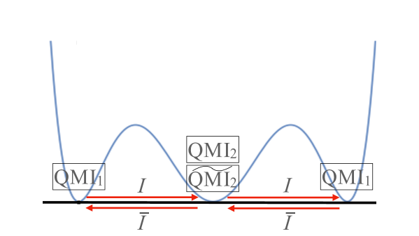
Figure 3: The each QMI exists between $I$ and $\bar{I}$ or $I(\bar{I})$ and $I(\bar{I})$. The effect of the deformed parameter $p$ is included in each QMI.

VI Median resummation of exact quantization condition

Let us reconsider the exact form of the quantization conditions. Although the exact form is given by Eqs. (82), (83) and is invariant under the DDP formula (84), i.e, ${\cal S}_{+}[{\mathfrak{D}}^{+}]={\cal S}_{-}[{\mathfrak{D}}^{-}]$, it is not very helpful expression because it is a function of ${\cal S}_{\pm}[{\mathfrak{A}}_{\ell}]$, which has a non-perturbative contribution in it, and the solutions are not automatically in the Borel-Ecalle resummed form which is free of ambiguities. Now, let us express the exact form as a function of $({\mathfrak{A}}_{\ell},{\mathfrak{B}}_{\ell})$.

In order to do so, we consider the median resummation using the Stokes automorphism ${\mathfrak{S}}$ which is defined as Ec1 ; 2014arXiv1405.0356S ; Dorigoni2019 ; Aniceto:2013fka

$${\cal S}_{+}={\cal S}_{-}\circ{\mathfrak{S}}.$$ (143)

Stokles automorphism can also be expressed through the Alien derivative ${\Delta}_{w}$ as

$${\mathfrak{S}}^{\nu}=\exp\left[\nu\sum_{w\in\Gamma}\overset{\underset{\bullet}{}}{\Delta}_{w}\right]=1+\sum_{k=1}^{\infty}\sum_{\{n_{1},\cdots,n_{k}\geq 1\}}\frac{\nu^{k}}{k!}\prod_{s=1}^{k}\overset{\underset{\bullet}{}}{\Delta}_{w_{n_{s}}},$$ (144)

$$\overset{\underset{\bullet}{}}{\Delta}_{w}:=e^{-w/\hbar}\Delta_{w},$$ (145)

where $\Gamma$ is the set of singular points on the positive real axis in the Borel plane, $w_{n}\in\Gamma$ is the $n$-th singular point given by $w_{n}=nS_{\rm B}$ with $S_{\rm B}$ denoting the bion action of $B$-cycles, and ${\mathfrak{S}}=:{\mathfrak{S}}^{+1}$. The alien derivative is a useful tool to probe the singularities in the Borel plane as described below. By defining the median resummation as

$${\cal S}_{\rm med}:={\cal S}_{+}\circ{\mathfrak{S}}^{-1/2}={\cal S}_{-}\circ{\mathfrak{S}}^{+1/2},$$ (146)

the quantization condition can be expressed by ${\mathfrak{D}}_{\rm ex}$ as

$${\mathfrak{D}}^{\pm}={\mathfrak{S}}^{\mp 1/2}[{\mathfrak{D}}_{\rm ex}]\quad\Rightarrow\quad{\mathfrak{D}}_{\rm ex}={\mathfrak{S}}^{\pm 1/2}[{\mathfrak{D}}^{\pm}].$$ (147)

Notice that ${\mathfrak{D}}_{\rm ex}$ in Eq.(147) is still an asymptotic expansion, which is a function of $({\mathfrak{A}}_{\ell},{\mathfrak{B}}_{\ell})$. But by replacing them with the Borel resummed form defined as

$${\mathfrak{A}}_{\ell} \rightarrow \widehat{\mathfrak{A}}_{\ell}:={\cal S}_{+}\circ{\mathfrak{S}}^{-1/2}[{\mathfrak{A}}_{\ell}]={\cal S}_{-}\circ{\mathfrak{S}}^{+1/2}[{\mathfrak{A}}_{\ell}],$$ (148)

$${\mathfrak{B}}_{\ell} \rightarrow \widehat{\mathfrak{B}}_{\ell}:={\cal S}_{+}\circ{\mathfrak{S}}^{-1/2}[{\mathfrak{B}}_{\ell}]={\cal S}_{-}\circ{\mathfrak{S}}^{+1/2}[{\mathfrak{B}}_{\ell}],$$ (149)

one can obtain the exact form of the quantization condition. It is notable that $\widehat{\mathfrak{A}}_{\ell}$ does not have the imaginary ambiguity, and $\widehat{\mathfrak{A}}_{\ell}(\hbar)\xrightarrow{\hbar\rightarrow 0_{+}}{\mathfrak{A}}_{\ell}(\hbar)$.

The Alien derivative acting on cycles and their Stokes automorphism are given by

Double-well $$: \quad\overset{\underset{\bullet}{}}{\Delta}_{w_{n}}{\mathfrak{A}}_{\ell}=\frac{(-1)^{n}}{n}{\mathfrak{A}}_{\ell}{\mathfrak{B}}^{n},\qquad\overset{\underset{\bullet}{}}{\Delta}_{w_{n}}{\mathfrak{B}}=0,$$ (151)

$$\quad{\mathfrak{S}}^{\nu}[{\mathfrak{A}}_{\ell}]={\mathfrak{A}}_{\ell}(1+{\mathfrak{B}})^{-\nu},\qquad{\mathfrak{S}}^{\nu}[{\mathfrak{B}}]={\mathfrak{B}},$$

Triple-well $$: \quad\overset{\underset{\bullet}{}}{\Delta}_{w_{n}}{\mathfrak{A}}_{2\ell-1}=\frac{(-1)^{n}}{n}{\mathfrak{A}}_{2\ell-1}{\mathfrak{B}}^{n}_{\ell},\qquad\overset{\underset{\bullet}{}}{\Delta}_{w_{n}}{\mathfrak{A}}_{2}=\frac{(-1)^{n}}{n}{\mathfrak{A}}_{2}({\mathfrak{B}}^{n}_{1}+{\mathfrak{B}}^{n}_{2}),$$ (153)

$$\quad\overset{\underset{\bullet}{}}{\Delta}_{w_{n}}{\mathfrak{B}}_{\ell}=0,$$

$$\quad{\mathfrak{S}}^{\nu}[{\mathfrak{A}}_{2\ell-1}]={\mathfrak{A}}_{2\ell-1}(1+{\mathfrak{B}}_{\ell})^{-\nu},\qquad{\mathfrak{S}}^{\nu}[{\mathfrak{A}}_{2}]={\mathfrak{A}}_{2}\prod_{\ell=1}^{2}(1+{\mathfrak{B}}_{\ell})^{-\nu},$$

$$\quad{\mathfrak{S}}^{\nu}[{\mathfrak{B}}_{\ell}]={\mathfrak{B}}_{\ell},$$

where $\ell\in\{1,2\}$. These relations are the hall-mark of resurgence, the fact that alien derivatives and Stokes automorphisms of perturbative series in a given saddle produce the series around the other saddles and nothing else. Also note that $\overset{\underset{\bullet}{}}{\Delta}_{w_{n}}{\mathfrak{B}}=0$ implies the perturbative expansion of $B$ cycle does not have singularities on positive real axis. Due to P-NP relation, we know that the $B$-cycle must also represent a divergent asymptotic expansion. The combination of these two facts implies that perturbation theory around the bion saddle must be Borel summable along positive real axis on Borel plane. On the other hand, it is expected to have singularities on the negative real axis. In comparison, perturbation theory around perturbative vacuum has infinitely many singularities on the positive real axis associated with bion configurations. As a result of these, the median resummation of quantization conditions ${\mathfrak{D}}_{\rm ex}$ can be expressed as:

Double-well $$: {\mathfrak{D}}_{\rm ex}=1+\frac{{\mathfrak{A}}_{1}}{{\mathfrak{A}}_{2}}+\left({\mathfrak{A}}_{1}+{\mathfrak{A}}^{-1}_{2}\right)\left(1+{\mathfrak{B}}\right)^{1/2}$$ (154)

$$\qquad=1+e^{-2i\pi p}+\left(e^{-\pi ip}\bar{\mathfrak{A}}+e^{-\pi ip}\bar{\mathfrak{A}}^{-1}\right)\left(1+\bar{\mathfrak{B}}\right)^{1/2},$$

Triple-well $$: {\mathfrak{D}}_{\rm ex}={\mathfrak{A}}_{2}^{-1}\prod_{\ell=1}^{2}\left[{\mathfrak{A}}_{2\ell-1}+\left(1+{\mathfrak{B}}_{\ell}\right)^{1/2}\right]+\prod_{\ell=1}^{2}\left[1+{\mathfrak{A}}_{2\ell-1}\left(1+{\mathfrak{B}}_{\ell}\right)^{1/2}\right]$$ (155)

$$\qquad={\mathfrak{A}}_{2}^{-1}\left[{\mathfrak{A}}_{1}+\left(1+{\mathfrak{B}}_{1}\right)^{1/2}\right]^{2}+\left[1+{\mathfrak{A}}_{1}\left(1+{\mathfrak{B}}_{1}\right)^{1/2}\right]^{2}\quad({\mathfrak{A}}_{1}={\mathfrak{A}}_{3},{\mathfrak{B}}_{1}={\mathfrak{B}}_{2})$$

$$\qquad=\prod_{\varepsilon\in\{-1,+1\}}\left[e^{3\pi ip/2}-i\varepsilon+\left(e^{\pi ip/2}\bar{\mathfrak{A}}^{-1}-i\varepsilon e^{\pi ip}\bar{\mathfrak{A}}\right)\left(1+\bar{\mathfrak{B}}\right)^{1/2}\right].$$

Now, we can obtain the non-perturbative contribution $\delta(\hbar)$ to the energy from ${\mathfrak{D}}_{\rm ex}$. For the double-well, it can be obtained as

Double-well :

$$\qquad\delta_{p\in{\mathbb{Z}}}(\hbar)={\cal P}\sqrt{\frac{{\mathfrak{B}}_{0}}{\pi\hbar\Gamma(1+k)\Gamma(1+k-p)}}\left(\frac{\hbar}{2}\right)^{-k+\frac{p}{2}}$$

$$\qquad\qquad\qquad\ -\frac{{\mathfrak{B}}_{0}}{\pi\hbar\Gamma(1+k)\Gamma(1+k-p)}\left(\frac{\hbar}{2}\right)^{-2k+p}\Phi_{0}(k,p)+O({\mathfrak{B}}_{0}^{3/2}),$$ (156)

$$\qquad\delta_{p\notin{\mathbb{Z}}}(\hbar)=(-1)^{1+k}\frac{{\mathfrak{B}}_{0}\Gamma(-k+p)}{\pi\hbar\Gamma(1+k)}\left(\frac{\hbar}{2}\right)^{-2k+p}\cos(\pi p)$$

$$\qquad\qquad\qquad\ -\frac{2{\mathfrak{B}}_{0}^{2}\Gamma(-k+p)^{2}}{\pi^{2}\hbar^{2}\Gamma(1+k)^{2}}\left(\frac{\hbar}{2}\right)^{-4k+2p}\cos^{2}(\pi p)\cdot\left[\Phi_{0}(k,p)-\frac{3\pi}{2}\tan(\pi p)\right]+O({\mathfrak{B}}_{0}^{3}),$$ (157)

where ${\cal P}\in\{-1,+1\}$ is parity, and $\Phi_{n}(k,p)$ is given by Eq.(94).

For the triple-well, we set $p=(2q+1)/3$. The non-perturbative contribution to the energies is given by

Triple-well (inner-vacuum) :

$$\qquad\delta^{\varepsilon=(-1)^{q}}_{k+q\in 2{\mathbb{Z}}+1}(\hbar)=0,$$ (158)

$$\qquad\delta^{\varepsilon=(-1)^{q+1}}_{k+q\in 2{\mathbb{Z}}+1}(\hbar)={\cal P}\sqrt{\frac{{\mathfrak{B}}_{0}}{\pi\Gamma(1+k)\Gamma(\frac{1}{2}+\frac{k}{2}-\frac{q}{2})}}2^{-\frac{1}{4}(2+k-q)}\hbar^{-\frac{1}{4}\left(1+3k-q\right)}$$ (159)

$$\qquad\qquad\qquad\qquad\quad-\frac{{\mathfrak{B}}_{0}2^{-\frac{1}{2}(2+k-q)}\hbar^{-\frac{1}{2}\left(1+3k-q\right)}}{2\pi\Gamma(1+k)\Gamma(\frac{1}{2}+\frac{k}{2}-\frac{q}{2})}\Psi^{(1)}_{0}\left(k,\frac{2q+1}{3}\right)+O({\mathfrak{B}_{0}^{3/2}}),$$ (160)

$$\qquad\delta_{k+q\notin 2{\mathbb{Z}}+1}(\hbar)=-\frac{{\mathfrak{B}}_{0}2^{-\frac{1}{2}(2+k-q)}\hbar^{-\frac{1}{2}(1+3k-q)}\Gamma(\frac{1}{2}-\frac{k}{2}+\frac{q}{2})}{\pi\Gamma(1+k)}\sin\frac{\pi(k-q)}{2}$$

$$\qquad\qquad\qquad\qquad\quad-\frac{{\mathfrak{B}}_{0}^{2}2^{-(2+k-q)}\hbar^{-(1+3k-q)}\Gamma(\frac{1}{2}-\frac{k}{2}+\frac{q}{2})^{2}}{\pi^{2}\Gamma(1+k)^{2}}\sin^{2}\frac{\pi(k-q)}{2}$$

$$\qquad\qquad\qquad\qquad\quad\cdot\left[\Psi^{(1)}_{0}\left(k,\frac{2q+1}{3}\right)-3\pi\cot\frac{\pi(k-q)}{2}\right]+O({\mathfrak{B}}_{0}^{3}),$$ (161)

Triple-well (outer-vacua) :

$$\qquad\delta^{\varepsilon=(-1)^{q}}_{q\in{\mathbb{Z}}}(\hbar)=0,$$ (162)

$$\qquad\delta^{\varepsilon=(-1)^{q+1}}_{q\in{\mathbb{Z}}}(\hbar)={\cal P}\sqrt{\frac{{\mathfrak{B}}_{0}}{\pi\Gamma(1+k)\Gamma(2+2k+q)}}2^{-\frac{1}{4}(3+2k)}\hbar^{-\frac{1}{2}\left(2+3k+q\right)}$$

$$\qquad\qquad\quad\quad\quad\quad\ \,\,-\frac{{\mathfrak{B}}_{0}2^{-\frac{1}{2}(3+2k)}\hbar^{-\left(2+3k+q\right)}}{2\pi\Gamma(1+k)\Gamma(2+2k+q)}\Psi^{(2)}_{0}\left(k,\frac{2q+1}{3}\right)+O({\mathfrak{B}_{0}^{3/2}}),$$ (163)

$$\qquad\delta_{q\notin{\mathbb{Z}}}(\hbar)=-\varepsilon\frac{{\mathfrak{B}}_{0}2^{-\frac{1}{2}(3+2k)}\hbar^{-(2+3k+q)}\Gamma(-1-2k-q)}{\pi\Gamma(1+k)}\left(\tan\frac{\pi q}{2}\right)^{\varepsilon}\sin(\pi q)$$

$$\qquad\qquad\qquad\ \,-\frac{{\mathfrak{B}}_{0}^{2}2^{-(3+2k)}\hbar^{-2(3k+q+2)}\Gamma(-1-2k-q)}{\pi^{2}\Gamma(1+k)^{2}}\left(\tan\frac{\pi q}{2}\right)^{2\varepsilon}\sin^{2}(\pi q)$$

$$\qquad\qquad\qquad\ \,\cdot\left[\Psi^{(2)}_{0}\left(k,\frac{2q+1}{3}\right)-3\pi\varepsilon\left(\cot\frac{\pi q}{2}\right)^{\varepsilon}\right]+O({\mathfrak{B}}_{0}^{3}),$$ (164)

where $\varepsilon\in\{-1,+1\}$, and $\Psi^{(1,2)}_{n}(k,p)$ are given by Eqs.(102) and (103).

Although these equations are very complicated,we can extract lots of nontrivial physical facts from them. From now on, we will show such facts one by one: Firstly, up to our knowledge, Eqs.(158)-(164) are the first results of non-perturbative contribution to energies with already built-in resurgent cancellation. Let us briefly explain this. In the standard discussions of resurgence in the QM context, one finds a non-perturbative ambiguity in the Borel resummation of perturbation theory, and then, one finds that the bion amplitudes are also two-fold ambiguous. Then, one shows that these two types of ambiguities cancel each other out leading to an ambiguity free result. Our formalism, the median resummation of the exact quantization condition already takes care of this process. All discontinuities, left/right resummation of perturbation theory, two-fold ambiguous bion amplitudes, or equivalently, the content of the DDP formula is taken into account. The outcome of the solution of median resummed exact quantization is already in an Borel-Ecalle resummed form.

The physical implications of (156) and (157) are succinctly explained in Fig. 2, and itemized in §.V.2.1 for the quantum deformed double-well potential. Indeed, we see that exact quantization conditions captures all non-trivial features of the whole spectrum, in particular the phenomenon of appearance (for $p\in{\mathbb{Z}}$) and disappearance (for $p\notin{\mathbb{Z}}$) of instanton contributions to the spectrum is neatly captured by the solution.

There is a very broad range of implications of Eqs.(158)-(164) for the spectrum of the quantum deformed triple-well potentials, and the result captures both perturbative and non-perturbative properties of different $q\in\mathbb{R}$ theories at once. We now describe them in turn Dunne:2020gtk ; Brezin:1977gk .

We start with a reminder of a fact. The energy levels for inner and outer harmonic vacua of quantum deformed triple-well systems is given in (88). Let us denote $p=\frac{2q+1}{3}$, and $q\in\mathbb{R}$. Perturbatively, there are two cases.

• For $q\in\mathbb{Z}$, half of the harmonic states in the central well are aligned with the harmonic states in the outer wells, as shown in Figs.4 and 5. This alignment holds to all orders in perturbation theory. We checked this by obtaining perturbation theory from A-cycles and also, by studying perturbation theory by using Bender-Wu package Sulejmanpasic:2016fwr .

• For $q\notin\mathbb{Z}$, the harmonic states in the central well are not aligned with the harmonic states in the outer wells.

Therefore, we expect significant differences in the spectral properties of the theories with $q\in\mathbb{Z}$ and $q\notin\mathbb{Z}$, and indeed, exact quantization condition reflects this. Non-perturbatively, the outcome of the spectral properties of the quantum deformed theory is depicted in Fig.6.

VI.1 Unquantized deformations or $q\notin\mathbb{Z}$ theories

Classical potential: First, note that the classical potential, corresponding to $p=0\;(q=-1/2)$ is an example of this class. In this case, the inner well energies at leading harmonic order are $E_{\rm in}=\frac{1}{2}\left(k_{\rm in}+\frac{1}{2}\right)=\left\{\frac{1}{4},\frac{3}{4},\frac{5}{4},\ldots\right\}$ and outer well energies are $E_{\rm out}=\left(k_{\rm out}+\frac{1}{2}\right)=\left\{\frac{1}{2},\frac{3}{2},\frac{5}{2},\ldots\right\}$. The inner and outer levels are never aligned. Only the last one of Eqs. Eqs.(158)-(164) apply. They imply that for the inner well, the leading non-perturbative contribution is bion, of order ${\mathfrak{B}}_{0}$, and leads to mere shift of the energy. For the outer well, the leading NP contribution is again bion, extrapolating between the outer degenerate vacua, and it leads to level splitting between parity even/odd states of order ${\mathfrak{B}}_{0}$.

The interesting point is that despite the fact that instantons are finite action saddles, there is no contribution to spectrum at the instanton level $\sqrt{{\mathfrak{B}}_{0}}$. This comes about because the inner and outer wells are not aligned. If one inspects the determinant of the fluctuation operator $F=-\frac{d^{2}}{d\tau^{2}}+V^{{}^{\prime\prime}}(x)|_{x_{\rm cl.}(\tau)}$ in an instanton background, it is infinite. As a result, the instanton amplitude is strictly zero. On the other hand, the fluctuation operator in the background of bions is finite.

Other $q\notin{\mathbb{Z}}$ cases: Just like the classical case, for all $q\notin{\mathbb{Z}}$ cases, there are no $\sqrt{{\mathfrak{B}}_{0}}\sim e^{-S_{\rm I}/\hbar}$ contribution to energy spectrum. Both energy shifts as well as level splittings (between degenerate states in the left/right outer vacua) are dictated by ${\mathfrak{B}}_{0}\sim e^{-2S_{\rm I}/\hbar}$.

VI.2 Quantized deformations or $q\in\mathbb{Z}$ theories

Figure 4: Perturbative spectrum of the triple-well potentials for non-negative integer values of $q$. The three-fold degeneracies are exact to all orders in perturbation theory. States in the blue shaded part have convergent/divergent pattern of perturbative expansion and in the red part, all perturbative expansion are asymptotic. Low levels only have bion non-perturbative contribution. Higher singlet states only have bion contributions, and perturbatively treefold degenerate states have both instanton and bion contribution.

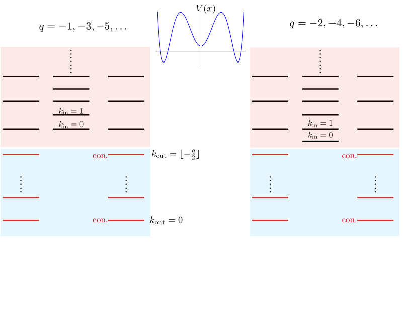
Figure 5: Perturbative spectrum of the triple-well potentials for negative integer values of $q$. The two-fold and three-fold degeneracies are exact to all orders in perturbation theory. States in the blue shaded part have all convergent perturbative expansion and in the red part, all perturbative expansion are asymptotic. Low levels either have no NP contribution (and those states are exactly solvable QES states) or bion NP contribution. Higher singlet states have bion contributions, and perturbatively treefold degenerate states have both instanton and bion contribution.

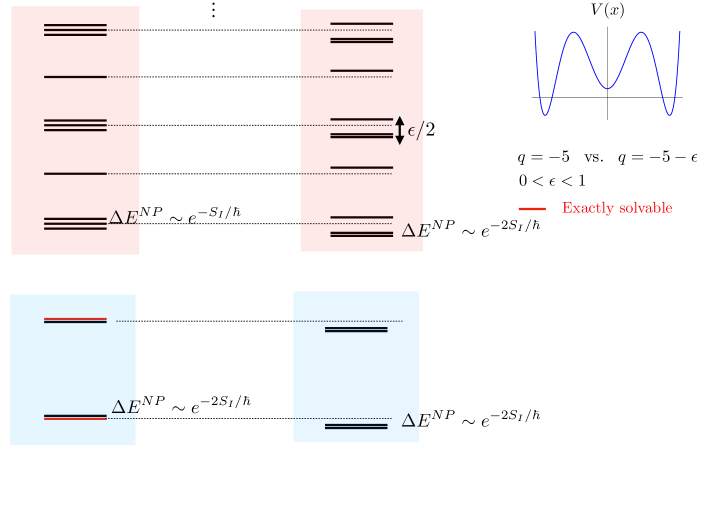
Figure 6: Non-Perturbative spectrum of the triple-well potentials for $q=-5$ and $q=-5-\epsilon$. For $q=-5$, two states on ${\cal H}_{0}$ (blue band) are exactly solvable, and they are separated from the perturbatively degenerate state by a bion effect $e^{-2S_{\rm I}/\hbar}$. The triple degeneracy at the upper band is lifted by instanton effect. For $q=-5-\epsilon$, where $\epsilon>e^{-S_{\rm I}/\hbar}$, the perturbative triplet is split to doublet (by $-\epsilon/3$) and singlet (by $\epsilon/6$). All double degeneracies in the spectrum are lifted by bion effects $e^{-2S_{\rm I}/\hbar}$. For $q\notin\mathbb{Z}$, there are no single instanton effects in the spectrum. For $\epsilon=1$, three states in the spectrum becomes exactly solvable, and this pattern continues.

Special theories $q\in\mathbb{Z}$: Triple well potentials for $q\in{\mathbb{Z}}$ are special. For example, $q=1$ and $q=-2$ correspond to $p=\pm 1$ which are supersymmetric pairs. The $q=2$ and $q=-3$ correspond to $p=\pm\frac{5}{3}$ which are QES systems. For integer $q$, the states in the outer well become degenerate with every other state in the inner well, and this degeneracy is an all orders statement in perturbation theory. The perturbative spectrum for these special cases are shown in Fig. 4 and Fig. 5.

For $q=1,3,5,\ldots$, calculating perturbation theory via either Bender-Wu package or using the perturbative $A$-cycle expansion yields an intriguing result. Levels with $k_{\rm in}=0,\ldots,q-1$ have a convergent/divergent alternating pattern. For $k_{\rm in}\geq q$, states have divergent asymptotic perturbative expansion.

Inspecting Eqs.(158)-(161), we indeed observe that due to the $\frac{1}{\Gamma(\frac{1}{2}+\frac{k_{\rm in}}{2}-\frac{q}{2})}$ factor, instanton factor proportional to $\sqrt{{\mathfrak{B}}_{0}}$ disappears for $k_{\rm in}\leq q-1$ and is present provided $k_{\rm in}\geq q$ and $\varepsilon=(-1)^{q+1}$ states. For $k_{\rm in}=q,q+2,\ldots$, the single states in red shaded region, the instanton factor does not appear and complex bion contribution vanishes according to exact quantization condition. Indeed, in the path integral formalism, we can actually show that the complex bion contribution appears as ${\mathfrak{B}}_{0}e^{\pm i\frac{\pi}{2}(q+1-k_{\rm in})}$ where the exponent is the hidden topological angle $\theta_{\rm HTA}$. For $k_{\rm in}=q,q+2,\ldots$, the real part of the complex bion contribution ${\rm Re}[{\mathfrak{B}}_{0}e^{\pm i\frac{\pi}{2}(q+1-k_{\rm in})}]=0$ is zero, there is a purely imaginary ambiguous part ${\rm Im}[{\mathfrak{B}}_{0}e^{\pm i\frac{\pi}{2}(q+1-k_{\rm in})}]\neq 0$, and that vanishes upon Borel-Ecalle resummation to cancel the ambiguity of perturbation theory.

For $k_{\rm in}=q+1,q+3,\ldots$, the triple-degenerate state states in red shaded region, the instanton factor appears. Note that the degeneracy is valid to all orders in perturbation theory. Since $q$ is odd, a harmonic central state which is part of a triplet is parity even. We can discuss the linear combinations of the harmonic states that appear as eigenstates of the Hamiltonian in simple terms. At leading order in semi-classics, the transfer matrix defined by tunneling among each wavefunction for the basis $\psi:=(\psi_{\rm L},\psi_{\rm C},\psi_{\rm R})^{\top}$,

$$\delta M:=\begin{pmatrix}0&&\delta_{\rm I}&&0\\ \delta_{\rm I}&&0&&\delta_{\rm I}\\ 0&&\delta_{\rm I}&&0\end{pmatrix},\qquad\delta_{\rm I}:=e^{-S_{\rm I}/\hbar},$$ (165)

where $\psi_{\rm C}$ is the locally defined wavefunction around the central-vacuum, and $\psi_{\rm L/R}$ are the ones around the left/right outer-vacua. The eigenvalues of $\delta M$ and their eigenvectors are given by

$${\rm Eigen}(\delta M)=\left\{\pm\sqrt{2}e^{-S_{\rm I}/\hbar},0\right\},$$ (166)

$$v_{\pm}=(1,\pm\sqrt{2},1)^{\top},\qquad v_{0}=(1,0,-1)^{\top}.$$ (167)

The eigenfunction can be found by linear combination of $\psi_{\rm L,C,R}$ as $v^{\top}\psi$, and one can see the fact that the energy shift in (159) and (163) is caused by $\delta\psi_{\pm}:=v^{\top}_{\pm}\psi$. Notice that $\psi_{\rm L}$ and $\psi_{\rm R}$ in $\delta\psi_{\pm}$ is symmetric, and thus the value of ${\cal P}$ is determined by the sign of $\pm\sqrt{2}\psi_{\rm C}$ in $\delta\psi_{\pm}$. Unlike $\psi_{\rm L,C,R}$, $\delta\psi_{\pm}$ can not be defined around each local vacuum, so one can only say that ${\cal P}_{\rm in}=-{\cal P}_{\rm out}$ and that ${\cal P}=\pm 1$ arises by $\delta\psi_{\pm}$. In the case of $\delta\psi_{0}:=v_{0}^{\top}\psi$, the $\psi_{\rm L}$ and $\psi_{\rm R}$ are antisymmetric each other and $\psi_{\rm C}$ does not enter into $\delta\psi_{0}$. Therefore, only $\delta^{\varepsilon=(-1)^{q}}_{q\in{\mathbb{Z}}}$ in (162) has to be taken into account and $\delta^{\varepsilon=(-1)^{q}}_{k+q\in 2{\mathbb{Z}}+1}$ in (158) is irrelevant to the zero-energy shift. It is consistent with the fact that the triple-well has three-fold energy degeneracy. In contrast to ${\cal P}$, $\varepsilon$ appears in the energy shift of the outer-vacua for any $q$ due to the parity symmetry of potential, i.e. $V(x,\hbar)=V(-x,\hbar)$, and is also relevant to the energy splitting by bion contribution between the left and right vacua. For $q\in{\mathbb{Z}}$, if $\varepsilon=(-1)^{q+1}$, then the wavefunctions of the left and right vacua reduce to the symmetric state giving the energy shift by the bion, otherwise the anti-symmetric state giving the zero-energy shift. It is remarkable to state that all $\delta\psi_{\pm,0}$ can be unifiedly expressed through ${\cal P}$ and $\varepsilon$;

$$\delta\psi_{\#}=\frac{1+(-1)^{q+1}\varepsilon}{\sqrt{2}}{\cal P}\psi_{\rm C}+\psi_{\rm L}+(-1)^{q+1}\varepsilon\psi_{\rm R},$$ (168)

$$\#=\begin{cases}+&\mbox{if}\quad{\cal P}=+1\quad\mbox{and}\quad\varepsilon=(-1)^{q+1}\\ -&\mbox{if}\quad{\cal P}=-1\quad\mbox{and}\quad\varepsilon=(-1)^{q+1}\\ 0&\mbox{if}\quad\varepsilon=(-1)^{q}\end{cases}.$$ (169)

As one can see from Eqs.(158) and (162), the non-perturbative contributions from the choice of $\varepsilon=(-1)^{q}$ with $q\in 2{\mathbb{Z}}+1$ and $q\in{\mathbb{Z}}$ for the inner vacuum and outer-vacua in the triple-well, respectively, vanish by performing the Borel resummation. These results are quite nontrivial in the sense that in general it is not quite enough to imagine the Borel resummed results only by taking look at the lower orders and their discontinuity (or imaginary ambiguity) in before-Borel resummed forms in Eqs.(96) and (99). Eqs.(96) and (99) indeed have a part without discontinuities in $O({\mathfrak{B}}^{2}_{0})$, but it also vanishes by the Borel resummation, which means that a resurgence relation such as the DDP formula has to be needed to consider a next-leading term or higher in general. In this sense, for a given function, the condition that it asymptotically gives a Borel non-summable perturbative power series is in general not a sufficient condition for the existence of higher transmonomials such as an exponentially small factors in the expansion.

VII Summary and Prospects

In this work, we generalized the exact-WKB analysis to quantum deformed potentials, $V(x,\hbar)=V_{0}(x)+\hbar pV_{1}(x)$, given in (1), where $V_{0}(x)$ is classical and $\hbar V_{1}(x)$ is quantum deformation. This class of systems are not rare. They are as typical as classical system, but received lesser attention. They arise naturally once the quantum mechanics of a bosonic field $x(\tau)$ is coupled to $N_{f}$ Grassmann valued field $\psi_{i}(\tau)$ or to topological Wess-Zumino terms for internal spin-$S$. In this class of theories, so far only ${\cal N}=1$ supersymmetric quantum mechanics received wide spread attention. However, all these theories have remarkable spectral properties, along with quite interesting non-perturbative aspects. In this work, we examined quantum deformed double- and triple-well quantum mechanics. Below, we summarize physically the most important outcome of our analysis and state some open issues.

Median resummation of exact quantization condition: Exact quantization condition is already discussed in literature, and here, we provided a streamlined derivation for the generic polynomial potentials. We argued that a more useful form of the exact quantization condition is its median resummed form in Eqs.(154)(155). The idea of median resummation is used earlier only in the important Pham et.al. DDP2 to show the reality of energy spectrum, but not used as a computational tool. In our work, solving the median resummed form, we obtained the non-perturbative correction to energy levels. The beauty of this formalism is that the resurgent cancellations that are usually taken into account only a posteriori and order by order (eg. between NP ambiguity of perturbation theory vs. two-fold ambiguity of bions, and then next level etc) is already built into the median resummed equation. The spectrum directly comes out to be as in Borel-Ecalle resummed form. Furthermore, the formalism also reveals some all order cancellations that are not easy to see in the standard approach.

Fading vs. Robust contributions in semi-classics: Assume, as it is the case in our examples, there are instanton solutions to the classical system with potential $V_{0}(x)={\textstyle{\frac{1}{2}}}W^{\prime}(x)^{2}$. These are also exact classical solutions in quantum deformed system, as the instanton equations $\dot{x}(\tau)=\pm W^{\prime}(x)$ do not care about $\hbar$ deformation. Yet, we learn that the instanton contribution at leading order in semi-classics $e^{-S_{\rm I}/\hbar}$ only takes place in special cases, and generically it is not there. Its contribution requires an exact alignment, that harmonic states in two consecutive wells must be exactly degenerate to all-orders in perturbation theory. For double-well, this happens only when $p\in{\mathbb{Z}}$ as shown in Eq.(92) and Eq.(93), and for triple well, it happens only when $q\in{\mathbb{Z}}$, where $p=\frac{2q+1}{3}$ as shown in Eqs.(96)-(99). If the quantum deformation term $p\in\mathbb{R}\setminus{\mathbb{Z}}$ for double-well and $q\in\mathbb{R}\setminus{\mathbb{Z}}$ for triple-well, instantons do not contribute to the energy spectrum at leading order $e^{-S_{\rm I}/\hbar}$. This is a natural conclusion of the exact-WKB formalism applied to quantum-deformed potentials, and solutions of exact quantization conditions. It would be nice to show this in full detail in path integral formulation. In particular, the quantization of the deformation parameter arises from the condition that harmonic levels in two consecutive wells must be the same. In path integral formulation, what must happen is that the fluctuation determinant in front of instanton amplitude must blow up if the consecutive states are not aligned, hence leading to the vanishing of instanton amplitude. Indeed, in a special case, this is observed to be the case Dunne:2020gtk . On the other hand, the energy spectrum has contributions of order $e^{-S_{\rm B}/\hbar}\sim e^{-2S_{\rm I}/\hbar}$ regardless of the value of the deformation parameter. In this sense, the contribution of instantons is fragile or fading, depends on precise alignment of states, yet the contribution of bions is robust.

HTA vs. Maslov index: Our construction does not imply that bion contributions never disappear. In fact, for triple-well, in the ${\cal N}=1$ SUSY case, there exists a supersymmetric ground state, hence, $E_{0}=0$ non-perturbatively. In this case, there are two types of bions, contributing to ground state and first excited state. The amplitudes of these two types of bions are identical, except a relative phase in between. If the relative phase is odd/even multiple $\pi$, it leads to destructive/constructive interference between them. In fact, for QES systems corresponding to $q=-2,-4,\ldots$ in Fig.5, there are $2\lfloor-\frac{q}{2}\rfloor$ states in the low end of the spectrum (denoted as ${\cal H}_{0}$ in (37)) for which perturbation theory is convergent. Half of these states are algebraically solvable with no non-perturbative contribution, and the other half receive NP bion contribution.

Resurgent structure for quantum deformed systems: The exact resurgent structure, where all the imaginary ambiguities are canceled between the perturbative and non-perturbative sectors, was obtained for quantum deformed double- and triple-well systems. For $q\in{\mathbb{Z}}$ (TW) and $p\in{\mathbb{Z}}$ (DW), states in ${\cal H}_{0}$ realizes Cheshire cat resurgence, namely, perturbation theory converges and ambiguities disappear, while states in ${\cal H}_{1}$ realized standard resurgence where ambiguities are cancelled between the perturbative and non-perturbative sectors. If $q\notin{\mathbb{Z}}$ (TW) and $p\notin{\mathbb{Z}}$ (DW), all states in ${\cal H}_{0}\oplus{\cal H}_{1}$ realize standard resurgent cancellations.

P-NP relation for bions: We proved by explicit computations that the perturbative fluctuations around the non-perturbative bion sectors is determined constructively by the perturbation theory around perturbative vacua for quantum deformed double- and triple-well systems. Since the symmetric triple well system can be practically reduced to a genus-1 system, and quantum deformation does not alter this property, the P-NP relations for both inner- and outer-energy are available, see (128) and (129), even when there is no alignment of the energy levels between the outer and inner well. One of the open interesting questions in this category is whether one can obtain a P-NP relation connecting different saddles constructively for higher genus potentials.

Appendix A Mellin transform

Firstly, we briefly review the essence of the Mellin transformZinn-Justin:2004qzw ; DP1 . The main point is that we transform a function $f(E)$ to a function of $s$ as $f(E)\rightarrow M(s)$ through an integration equipped with a measure $E^{-s-1}$. $f(E)$ can be reproduced from $M(s)$ by an inverse transform:

$$M(s)=\int^{L}_{0}E^{-s-1}f(E)dE,\qquad f(E)=\frac{1}{2\pi i}\int^{c+i\infty}_{c-i\infty}M(s)E^{s}ds.$$ (170)

For example, if $f(E)$ is a monomial of $E$ and $\log E$,

$$f(E)=E^{n}\quad(n>0):$$

$$\qquad\qquad M(s)=\int^{L}_{0}E^{n-s-1}dE=\frac{L^{n-s}}{n-s}=\sum_{\ell=0}^{\infty}\frac{(\log L)^{\ell}}{\ell!(n-s)^{-\ell+1}}$$

$$\qquad\qquad\qquad\ \,\rightarrow\quad\frac{1}{n-s}\quad\mbox{for \ $L=1$},$$ (171)

$$f(E)=E^{n}(\log E)^{m}\quad(n>0,m\in{\mathbb{N}});$$

$$\qquad\qquad M(s)=\int^{L}_{0}E^{n-s-1}(\log E)^{m}dE=\sum_{\ell=0}^{\infty}\sum_{k=0}^{m}\frac{m!}{k!}\frac{(-1)^{k+m}(\log L)^{\ell}}{(\ell-k)!(n-s)^{-\ell+m+1}}$$

$$\qquad\qquad\qquad\ \,\rightarrow\quad\frac{(-1)^{m}m!}{(n-s)^{m+1}}\quad\mbox{for \ $L=1$}.$$ (172)

By looking at the location of poles and its order in $M(s)$, one can easily reproduce $f(E)$.

A.1 Solutions of $M_{n}[\log\bar{B}](s)$

In order to consider the reduction of a $B$-cycle from the Airy-type to the DW-type, one needs to consider the Mellin transform defined as

$$M[\log\bar{B}](s,\hbar):=\oint_{\gamma_{\mathfrak{B}}}dx\,M[S^{\rm Airy}_{\rm odd}](x,s,\hbar)=\sum_{n=-1}^{\infty}\hbar^{n}M_{n}[\log\bar{B}](s),$$ (173)

where ${\bar{B}}({\cal E},\hbar)$ is a $B$-cycle given by the Airy-type as

$$\log\bar{B}({\cal E},\hbar):=\oint_{\gamma_{\mathfrak{B}}}dx\,S^{\rm Airy}_{\rm odd}(x,{\cal E},\hbar),$$ (174)

and ${\cal E}$ is the energy. In addition, the integration contour of the $B$-cycle, $\gamma_{\mathfrak{B}}$, is defined to be the same one as the case of the DW-type by taking ${\cal E}\rightarrow 0_{+}$.

We would write the solution of $M[\log\bar{B}](s,\hbar)$ in Eq.(173) below.

A.1.1 Tilted double-well

$$M_{-1}[\log\bar{B}](s)=-\frac{2^{3s-2}\sqrt{\pi}\Gamma(1-s)\Gamma(-s)}{\Gamma\left(-2s+\frac{5}{2}\right)},$$ (175)

$$M_{0}[\log\bar{B}](s)=0,$$ (176)

$$M_{1}[\log\bar{B}](s)=\frac{8^{s}\sqrt{\pi}\Gamma(-s-1)\Gamma(-s)}{\Gamma\left(-2s-\frac{1}{2}\right)}\left(-p^{2}+\frac{2s}{3}+1\right),$$ (177)

$$M_{2}[\log\bar{B}](s)=0,$$ (178)

$$M_{3}[\log\bar{B}](s)=-\frac{2^{3s+1}\sqrt{\pi}\Gamma(-s-3)\Gamma(-s)}{\Gamma\left(-2s-\frac{7}{2}\right)}\left(p^{4}-\frac{4p^{2}s}{3}+6p^{2}+\frac{28s^{2}}{45}+\frac{152s}{45}+5\right),$$ (179)

$$M_{4}[\log\bar{B}](s)=0,$$ (180)

$$M_{5}[\log\bar{B}](s)=\frac{8^{s+1}\sqrt{\pi}\Gamma(-s-5)\Gamma(-s)^{s}}{\Gamma\left(-2s-\frac{13}{2}\right)}$$

$$\qquad\qquad\qquad\quad\cdot\left(-\frac{p^{6}}{3}+\frac{2p^{4}s}{3}+5p^{4}-\frac{28p^{2}s^{2}}{45}-\frac{64p^{2}s}{9}-\frac{67p^{2}}{3}+\frac{248s^{3}}{945}+\frac{988s^{2}}{315}+\frac{11866s}{945}+\frac{53}{3}\right).$$

A.1.2 Tilted triple-well

$$M_{-1}[\log\bar{B}](s)=-\frac{3\ 2^{s-1}\Gamma(1-s)\Gamma(2-s)\Gamma(-s)}{\Gamma(4-3s)},$$ (182)

$$M_{0}[\log\bar{B}](s)=0,$$ (183)

$$M_{1}[\log\bar{B}](s)=\frac{2^{s-3}\Gamma(-s-1)\Gamma(-s)^{2}}{\Gamma(-3s-1)}\left(-3p^{2}+2s+3\right),$$ (184)

$$M_{2}[\log\bar{B}](s)=-\frac{2^{s-3}\Gamma(-s-2)\Gamma(-s-1)\Gamma(-s)}{\Gamma(-3(s+1))}p\left(p^{2}-1\right),$$ (185)

$$M_{3}[\log\bar{B}](s)=\frac{2^{s-6}(s+3)\Gamma(-s-3)^{2}\Gamma(-s)}{15\Gamma(-3(s+2))}$$

$$\qquad\qquad\qquad\quad\cdot\left(45p^{4}-60p^{2}s-270p^{2}+28s^{2}+152s+225\right),$$ (186)

$$M_{4}[\log\bar{B}](s)=\frac{2^{s-5}\Gamma(-s-4)^{2}\Gamma(-s)}{3(3s+8)\Gamma(-3(s+3))}p\left(p^{2}-1\right)(s+4)\left(-3p^{2}+2s+15\right),$$ (187)

$$M_{5}[\log\bar{B}](s)=\frac{2^{s-8}\Gamma(-s-5)^{2}\Gamma(-s)}{(3s+10)(3s+11)(3s+13)(3s+14)\Gamma(-3(s+5))}$$

$$\qquad\qquad\qquad\quad\cdot\left(p^{6}s+\frac{23p^{6}}{9}-2p^{4}s^{2}-21p^{4}s-\frac{385p^{4}}{9}+\frac{28p^{2}s^{3}}{15}+\frac{404p^{2}s^{2}}{15}\right.$$

$$\left.\qquad\qquad\qquad\qquad+131p^{2}s+\frac{1781p^{2}}{9}-\frac{248s^{4}}{315}-\frac{4772s^{3}}{405}-\frac{62338s^{2}}{945}-\frac{470413s}{2835}-\frac{473}{3}\right).$$ (188)

A.2 Derivation of $\bar{G}(E,\hbar)$

A.2.1 Tilted double-well

We consider how to calculate $\bar{G}(E,\hbar)$ in $\bar{\mathfrak{B}}(E,\hbar)$ below. We begin with the Airy-type Schrödinger equation with the energy ${\cal E}$. The $B$-cycle can be calculated as through the Mellin transform and is given by

$$\log\bar{B}({\cal E},\hbar) := \oint_{\gamma_{\mathfrak{B}}}dx\,S^{\rm Airy}_{\rm odd}(x,{\cal E},\hbar)$$ (189)

$$= -\frac{S_{\rm B}}{\hbar}+\sum_{n=0}^{\infty}\sum_{\ell=-n+1}^{\infty}{\cal E}^{\ell}\hbar^{n-1}\left(\alpha_{n,\ell}+\beta_{n,\ell}\log{\cal E}\right).$$

The first few non-zero coefficients are computed as

$$\alpha_{0,1}=2+2\log 2,\quad\alpha_{0,2}=-17+6\log 2,\quad\alpha_{0,3}=-236+70\log 2,$$

$$\beta_{0,1}=-2,\quad\beta_{0,2}=-6,\quad\beta_{0,3}=-70,$$

$$\alpha_{2,-1}=\frac{1}{12}-\frac{p^{2}}{4},\quad\alpha_{2,0}=\frac{3p^{2}}{2}-\frac{p^{2}}{2}\log 2-\frac{11}{6}+\frac{1}{2}\log 2,$$

$$\alpha_{2,1}=\frac{109p^{2}}{4}-\frac{15p^{2}}{2}\log 2-\frac{605}{12}+\frac{25}{2}\log 2,$$

$$\beta_{2,-1}=0,\quad\beta_{2,0}=\frac{p^{2}}{2}-\frac{1}{2},\quad\beta_{2,1}=\frac{15p^{2}}{2}-\frac{25}{2},$$

and one finds $S_{\rm B}=\frac{1}{3}$. Replacing the energy with ${\cal E}=E\hbar$ gives

$$\log\bar{B}(E\hbar,\hbar) = -\frac{S_{\rm B}}{\hbar}+\sum_{n=0}^{\infty}\sum_{\ell=-n+1}^{\infty}E^{\ell}\hbar^{n+\ell-1}\left[\alpha_{n,\ell}+\beta_{n,\ell}\log(E\hbar)\right]$$ (190)

$$= -\frac{S_{\rm B}}{\hbar}+\sum_{n=0}^{\infty}\sum_{\ell=0}^{\infty}E^{n-\ell+1}\hbar^{n}\left[\alpha_{\ell,n-\ell+1}+\beta_{\ell,n-\ell+1}\log(E\hbar)\right].$$

In order to obtain $\bar{G}$ from Eq.(190), we rewrite Eq.(114) as

$$\log\bar{\mathfrak{B}}(E,\hbar) = -\bar{G}(E,\hbar)-\sum_{s\in\{-1,+1\}}\log\Gamma\left(\frac{1+sp}{2}-\bar{F}(E,\hbar)\right)$$ (191)

$$+\log(2\pi)+2\bar{F}(E,\hbar)\log\left(\frac{\hbar}{2}\right),$$

and take the asymptotic expansion firstly for $E\rightarrow+\infty$, and then for $\hbar\rightarrow 0_{+}$. Since the asymptotic expansion of the $\Gamma$ function gives

$$\log\Gamma(z+p)=\left(z+p-\frac{1}{2}\right)\log z-z+\frac{1}{2}\log(2\pi)+\sum_{k=1}^{\infty}\frac{(-1)^{k+1}B_{k+1}(p)}{k(k+1)}z^{-k},$$ (192)

$$B_{n}(p)=\sum_{k=0}^{n}\begin{pmatrix}n\\ k\end{pmatrix}B_{k}p^{n-k},$$ (193)

where $B_{n}(x)$ is the Bernoulli polynomial with the Bernoulli number $B_{n}=B_{n}(0)$, it can be expressed by

$$\log\Gamma\left(\frac{1\pm p}{2}-\bar{F}(E,\hbar)\right) = \log\Gamma\left(p_{\pm}-\bar{F}(E,\hbar)\right)\qquad\left(p_{\pm}:=\frac{1\pm p}{2}\right)$$ (194)

$$= \left(-\bar{F}(E,\hbar)\pm\frac{p}{2}\right)\log(-\bar{F}(E,\hbar))+\bar{F}(E,\hbar)$$

$$+\frac{1}{2}\log(2\pi)+\sum_{k=1}^{\infty}\frac{(-1)^{k+1}B_{k+1}(p_{\pm})}{k(k+1)}(-\bar{F}(E,\hbar))^{-k}.$$

Thus,

$$\sum_{s\in\{-1,+1\}}\log\Gamma\left(\frac{1+sp}{2}-\bar{F}(E,\hbar)\right)$$ (195)

$$= -2\bar{F}(E,\hbar)\log(-\bar{F}(E,\hbar))+2\bar{F}(E,\hbar)$$

$$+\log(2\pi)+\sum_{k=1}^{\infty}\frac{(-1)^{k+1}(B_{k+1}(p_{+})+B_{k+1}(p_{-}))}{k(k+1)}(-\bar{F}(E,\hbar))^{-k}.$$

As a result, Eq.(191) can be written down as

$$\log\bar{\mathfrak{B}}(E,\hbar) = -\bar{G}(E,\hbar)+2\bar{F}(E,\hbar)\log\left(\frac{\hbar}{2}\right)$$ (196)

$$+2\bar{F}(E,\hbar)\log(-\bar{F}(E,\hbar))-2\bar{F}(E,\hbar)$$

$$+\sum_{k=1}^{\infty}\frac{(-1)^{k}(B_{k+1}(p_{+})+B_{k+1}(p_{-}))}{k(k+1)}(-\bar{F}(E,\hbar))^{-k}.$$

Finally, we connect Eqs.(190) and (196) to each other. By considering the asymptotic expansion in terms of $E$ for $\bar{F}(E,\hbar)$ as

$$\log\left(-\bar{F}(E,\hbar)\right) = \log E-\sum_{n=1}^{\infty}\frac{1}{n}\left(\frac{\bar{F}_{>0}(E,\hbar)}{E}\right)^{n},$$

$$(-\bar{F}(E,\hbar))^{-k} = \frac{1}{E^{k}}\left[\sum_{\ell=0}^{\infty}\left(\frac{\bar{F}_{>0}(E,\hbar)}{E}\right)^{\ell}\right]^{k},$$ (197)

where $\bar{F}_{0}(E)=-E,\bar{F}_{>0}(E,\hbar):=\bar{F}(E,\hbar)-\bar{F}_{0}(E)$, it can be written as

$$-\frac{S_{\rm B}}{\hbar}+\sum_{n=0}^{\infty}\sum_{\ell=0}^{\infty}E^{n-\ell+1}\hbar^{n}\left[\alpha_{\ell,n-\ell+1}+\beta_{\ell,n-\ell+1}\log(E\hbar)\right]$$ (198)

$$= -\bar{G}(E,\hbar)+2\bar{F}(E,\hbar)\left[\log\frac{E\hbar}{2}-\sum_{n=1}^{\infty}\frac{1}{n}\left(\frac{\bar{F}_{>0}(E,\hbar)}{E}\right)^{n}-1\right]$$

$$+\sum_{k=1}^{\infty}\frac{(-1)^{k}(B_{k+1}(p_{+})+B_{k+1}(p_{-}))}{k(k+1)}\frac{1}{E^{k}}\left[\sum_{\ell=0}^{\infty}\left(\frac{\bar{F}_{>0}(E,\hbar)}{E}\right)^{\ell}\right]^{k}.$$

We put the ansatz for $\bar{G}(E,\hbar)$ as

$$\bar{G}(E,\hbar)=\sum_{n=-1}^{\infty}\bar{G}_{n}(E)\hbar^{n}.$$ (199)

By comparing terms coupling with $\log(E\hbar)$ in both hand sides, one finds that ${\beta}_{n,\ell}$ is essentially identical to $\bar{F}(E,\hbar)$,

$$2\bar{F}(E,\hbar)=\sum_{n=0}^{\infty}\sum_{\ell=0}^{\infty}\beta_{\ell,n-\ell+1}E^{n-\ell+1}\hbar^{n}.$$ (200)

Therefore,

$$\bar{G}(E,\hbar) = \frac{S_{\rm B}}{\hbar}-\sum_{n=0}^{\infty}\sum_{\ell=0}^{\infty}\alpha_{\ell,n-\ell+1}E^{n-\ell+1}\hbar^{n}$$ (201)

$$-2\bar{F}(E,\hbar)\left[1+\log 2+\sum_{n=1}^{\infty}\frac{1}{n}\left(\frac{\bar{F}_{>0}(E,\hbar)}{E}\right)^{n}\right]$$

$$+\sum_{k=1}^{\infty}\frac{(-1)^{k}(B_{k+1}(p_{+})+B_{k+1}(p_{-}))}{k(k+1)}\frac{1}{E^{k}}\left[\sum_{\ell=0}^{\infty}\left(\frac{\bar{F}_{>0}(E,\hbar)}{E}\right)^{\ell}\right]^{k}.$$

A.2.2 Tilted triple-well

In the similar way to the double-well, $\bar{G}(E,\hbar)$ is available by using $B$-cycle given by the Airy-type and the Mellin transform. It is given by

$$\log\bar{B}(E\hbar,\hbar) = -\frac{S_{\rm B}}{\hbar}+\sum_{n=0}^{\infty}\sum_{\ell=-n+1}^{\infty}E^{\ell}\hbar^{n+\ell-1}\left[\alpha_{n,\ell}+\beta_{n,\ell}\log(E\hbar)\right]$$ (202)

$$= -\frac{S_{\rm B}}{\hbar}+\sum_{n=0}^{\infty}\sum_{\ell=0}^{\infty}E^{n-\ell+1}\hbar^{n}\left[\alpha_{\ell,n-\ell+1}+\beta_{\ell,n-\ell+1}\log(E\hbar)\right].$$

where $S_{\rm B}=\frac{1}{4}$. We rewrite Eq.(115) as

$$\log\bar{\mathfrak{B}}(E,\hbar) = -\bar{G}(E,\hbar)-\log\Gamma\left(\frac{1-p}{2}-\bar{F}(E,\hbar)\right)-\log\Gamma\left(\frac{1+p}{2}-2\bar{F}(E,\hbar)\right)$$ (203)

$$+\log(2\pi)+\left(\bar{F}(E,\hbar)+\frac{p}{2}\right)\log 2+3\bar{F}(E,\hbar)\log\hbar.$$

Since the gamma function can be written by

$$\log\Gamma\left(\frac{1-p}{2}-\bar{F}(E,\hbar)\right)+\log\Gamma\left(\frac{1+p}{2}-2\bar{F}(E,\hbar)\right)$$

$$= -3\bar{F}(E,\hbar)\log(-\bar{F}(E,\hbar))+\left(-2\bar{F}(E,\hbar)+\frac{p}{2}\right)\log 2+3\bar{F}(E,\hbar)$$

$$+\log(2\pi)+\sum_{k=1}^{\infty}\frac{(-1)^{k+1}}{k(k+1)}\left(B_{k+1}(p_{-})(-\bar{F}(E,\hbar))^{-k}+B_{k+1}(p_{+})(-2\bar{F}(E,\hbar))^{-k}\right),$$

one finds that Eq.(203) can be written down as

$$\log\bar{\mathfrak{B}}(E,\hbar) = -\bar{G}(E,\hbar)+3\bar{F}(E,\hbar)\left[\log(-2\bar{F}(E,\hbar)\hbar)-1\right]$$

$$+\sum_{k=1}^{\infty}\frac{(-1)^{k}}{k(k+1)}\left(B_{k+1}(p_{-})(-\bar{F}(E,\hbar))^{-k}+B_{k+1}(p_{+})(-2\bar{F}(E,\hbar))^{-k}\right).$$

By using the symbol as $\bar{F}_{0}(E)=-E,\bar{F}_{>0}(E,\hbar):=\bar{F}(E,\hbar)-\bar{F}_{0}(E)$, it can be expressed as

$$-\frac{S_{\rm B}}{\hbar}+\sum_{n=0}^{\infty}\sum_{\ell=0}^{\infty}E^{n-\ell+1}\hbar^{n}\left[\alpha_{\ell,n-\ell+1}+\beta_{\ell,n-\ell+1}\log(E\hbar)\right]$$ (206)

$$= -\bar{G}(E,\hbar)+3\bar{F}(E,\hbar)\left[\log(2E\hbar)-\sum_{n=1}^{\infty}\frac{1}{n}\left(\frac{\bar{F}_{>0}(E,\hbar)}{E}\right)^{n}-1\right]$$

$$+\sum_{k=1}^{\infty}\frac{(-1)^{k}}{k(k+1)}\left(\frac{B_{k+1}(p_{-})}{E^{k}}+\frac{B_{k+1}(p_{+})}{(2E)^{k}}\right)\left[\sum_{\ell=0}^{\infty}\left(\frac{\bar{F}_{>0}(E,\hbar)}{E}\right)^{\ell}\right]^{k}.$$

We put the ansatz for $\bar{G}(E,\hbar)$ as

$$\bar{G}(E,\hbar)=\sum_{n=-1}^{\infty}\bar{G}_{n}(E)\hbar^{n}.$$ (207)

By comparing terms coupling with $\log(E\hbar)$ in both hand sides, one finds that ${\beta}_{n,\ell}$ is essentially identical to $\bar{F}(E,\hbar)$,

$$3\bar{F}(E,\hbar)=\sum_{n=0}^{\infty}\sum_{\ell=0}^{\infty}\beta_{\ell,n-\ell+1}E^{n-\ell+1}\hbar^{n}.$$ (208)

Therefore,

$$\bar{G}(E,\hbar) = \frac{S_{\rm B}}{\hbar}-\sum_{n=0}^{\infty}\sum_{\ell=0}^{\infty}\alpha_{\ell,n-\ell+1}E^{n-\ell+1}\hbar^{n}$$ (209)

$$-3\bar{F}(E,\hbar)\left[1-\log 2+\sum_{n=1}^{\infty}\frac{1}{n}\left(\frac{\bar{F}_{>0}(E,\hbar)}{E}\right)^{n}\right]$$

$$+\sum_{k=1}^{\infty}\frac{(-1)^{k}}{k(k+1)}\left(B_{k+1}(p_{-})+\frac{B_{k+1}(p_{+})}{2^{k}}\right)\frac{1}{E^{k}}\left[\sum_{\ell=0}^{\infty}\left(\frac{\bar{F}_{>0}(E,\hbar)}{E}\right)^{\ell}\right]^{k}.$$

References

- (1) Berry and Mount, “Semiclassical approximations in wave mechanics,” 35 no. 1, (1972) 315–397.
- (2) H. J. Silverstone, “Jwkb connection-formula problem revisited via borel summation,” Phys. Rev. Lett. 55 (Dec, 1985) 2523–2526. https://link.aps.org/doi/10.1103/PhysRevLett.55.2523.
- (3) R. Balian, G. Parisi, and A. Voros, “Discrepancies from asymptotic series and their relation to complex classical trajectories,” Phys. Rev. Lett. 41 (Oct, 1978) 1141–1144. https://link.aps.org/doi/10.1103/PhysRevLett.41.1141.
- (4) A. Voros, “The return of the quartic oscillator. the complex wkb method,” Annales de l’I.H.P. Physique théorique 39 no. 3, (1983) 211–338. http://eudml.org/doc/76217.
- (5) E. Delabaere, H. Dillinger, and F. Pham, “Exact semiclassical expansions for one-dimensional quantum oscillators,” J. Math. Phys. 38 no. 12, (1997) 6126–6184.
- (6) E. Delabaere and F. Pham, “Resurgent methods in semiclassical asymptotics,” Ann. Inst. H. Poincare 71 (1999) 1–94.
- (7) Y. Takei, “An explicit description of the connection formula for the first Painleve equation, Toward the Exact WKB Analysis of Differential Equations,” Linear or Non-Linear, Kyoto Univ. Press (2000) 271–296.
- (8) Y. Takei, “Sato’s conjecture for the Weber equation and transformation theory for Schrödinger equations with a merging pair of turning points,” RIMS Kokyuroku Bessatsu B10 (2008) 205–224.
- (9) Y. Takei, “On the connection formula for the first Painleve equation : from the viewpoint of the exact WKB analysis(Painleve Transcendents and Asymptotic Analysis),” Kyoto University Research Information Repository 931 (1995) 70–99.
- (10) T. Kawai and Y. Takei, “Algebraic Analysis of Singular Perturbation Theory,” Providence, R.I. : American Mathematical Society c2005 .
- (11) T. Aoki, T. Kawai, and Y. Takei, “The Bender-Wu analysis and the Voros theory. II,” Adv. Stud. Pure Math. (Math. Soc. Japan) 54 (2009) 19–94.
- (12) A. Fruchard and R. Schafke, Asymptotics in Dynamics, Geometry and PDEs; Generalized Borel Summation vol. II. 2010.
- (13) K. Iwaki and T. Nakanishi, “Exact WKB analysis and cluster algebras,” J. Phys. A: Math. Theor. 47 (2014) 474009, arXiv:1401.709.
- (14) G. Alvarez, “Langer-Cherry derivation of the multi-instanton expansion for the symmetric double well.,” Journal of mathematical physics 45.8 (2004) 3095.
- (15) J. Zinn-Justin and U. D. Jentschura, “Multi-instantons and exact results I: Conjectures, WKB expansions, and instanton interactions,” Annals Phys. 313 (2004) 197–267, arXiv:quant-ph/0501136.
- (16) J. Zinn-Justin and U. D. Jentschura, “Multi-instantons and exact results II: Specific cases, higher-order effects, and numerical calculations,” Annals Phys. 313 (2004) 269–325, arXiv:quant-ph/0501137.
- (17) G. V. Dunne and M. Ünsal, “Generating nonperturbative physics from perturbation theory,” Phys. Rev. D 89 no. 4, (2014) 041701, arXiv:1306.4405 [hep-th].
- (18) G. V. Dunne and M. Unsal, “Uniform WKB, Multi-instantons, and Resurgent Trans-Series,” Phys. Rev. D 89 no. 10, (2014) 105009, arXiv:1401.5202 [hep-th].
- (19) N. A. Nekrasov and S. L. Shatashvili, “Quantization of Integrable Systems and Four Dimensional Gauge Theories,” in 16th International Congress on Mathematical Physics, pp. 265–289. 8, 2009. arXiv:0908.4052 [hep-th].
- (20) A. Mironov and A. Morozov, “Nekrasov Functions and Exact Bohr-Zommerfeld Integrals,” JHEP 04 (2010) 040, arXiv:0910.5670 [hep-th].
- (21) D. Gaiotto, G. W. Moore, and A. Neitzke, “Spectral networks,” Annales Henri Poincare 14 (2013) 1643–1731, arXiv:1204.4824 [hep-th].
- (22) P. Dorey, C. Dunning, and R. Tateo, “Spectral equivalences, Bethe Ansatz equations, and reality properties in PT-symmetric quantum mechanics,” J. Phys. A 34 (2001) 5679–5704, arXiv:hep-th/0103051.
- (23) P. Dorey, C. Dunning, and R. Tateo, “The ODE/IM Correspondence,” J. Phys. A 40 (2007) R205, arXiv:hep-th/0703066.
- (24) A. Grassi, M. Marino, and S. Zakany, “Resumming the string perturbation series,” JHEP 05 (2015) 038, arXiv:1405.4214 [hep-th].
- (25) A. Grassi, Y. Hatsuda, and M. Marino, “Topological Strings from Quantum Mechanics,” Annales Henri Poincare 17 no. 11, (2016) 3177–3235, arXiv:1410.3382 [hep-th].
- (26) A.-K. Kashani-Poor and J. Troost, “Pure super Yang-Mills and exact WKB,” JHEP 08 (2015) 160, arXiv:1504.08324 [hep-th].
- (27) A.-K. Kashani-Poor, “Quantization condition from exact WKB for difference equations,” JHEP 06 (2016) 180, arXiv:1604.01690 [hep-th].
- (28) S. K. Ashok, D. P. Jatkar, R. R. John, M. Raman, and J. Troost, “Exact WKB analysis of = 2 gauge theories,” JHEP 07 (2016) 115, arXiv:1604.05520 [hep-th].
- (29) K. Ito, M. Mariño, and H. Shu, “TBA equations and resurgent Quantum Mechanics,” JHEP 01 (2019) 228, arXiv:1811.04812 [hep-th].
- (30) L. Hollands and A. Neitzke, “Exact WKB and abelianization for the equation,” Commun. Math. Phys. 380 no. 1, (2020) 131–186, arXiv:1906.04271 [hep-th].
- (31) S. K. Ashok, P. N. Bala Subramanian, A. Bawane, D. Jain, D. P. Jatkar, and A. Manna, “Exact WKB Analysis of Holomorphic Blocks,” JHEP 10 (2019) 075, arXiv:1907.05031 [hep-th].
- (32) K. Ito and H. Shu, “TBA equations for the Schrödinger equation with a regular singularity,” J. Phys. A 53 no. 33, (2020) 335201, arXiv:1910.09406 [hep-th].
- (33) K. Imaizumi, “Exact WKB analysis and TBA equations for the Mathieu equation,” Phys. Lett. B 806 (2020) 135500, arXiv:2002.06829 [hep-th].
- (34) I. Coman, P. Longhi, and J. Teschner, “From quantum curves to topological string partition functions II,” arXiv:2004.04585 [hep-th].
- (35) D. G. L. Allegretti, “On the wall-crossing formula for quadratic differentials,” arXiv:2006.08059 [math.GT].
- (36) T. Kuwagaki, “Sheaf quantization from exact WKB analysis,” arXiv:2006.14872 [math.SG].
- (37) Y. Emery, “TBA equations and quantization conditions,” JHEP 07 (2021) 171, arXiv:2008.13680 [hep-th].
- (38) S. Enomoto and T. Matsuda, “The exact WKB for cosmological particle production,” JHEP 03 (2021) 090, arXiv:2010.14835 [hep-ph].
- (39) H. Taya, T. Fujimori, T. Misumi, M. Nitta, and N. Sakai, “Exact WKB analysis of the vacuum pair production by time-dependent electric fields,” JHEP 03 (2021) 082, arXiv:2010.16080 [hep-th].
- (40) F. Yan, “Exact WKB and the quantum Seiberg-Witten curve for 4d pure Yang-Mills, Part I: Abelianization,” arXiv:2012.15658 [hep-th].
- (41) Z. Duan, J. Gu, Y. Hatsuda, and T. Sulejmanpasic, “Instantons in the Hofstadter butterfly: difference equation, resurgence and quantum mirror curves,” JHEP 01 (2019) 079, arXiv:1806.11092 [hep-th].
- (42) N. Sueishi, S. Kamata, T. Misumi, and M. Ünsal, “On exact-WKB analysis, resurgent structure, and quantization conditions,” JHEP 12 (2020) 114, arXiv:2008.00379 [hep-th].
- (43) N. Sueishi, S. Kamata, T. Misumi, and M. Ünsal, “Exact-WKB, complete resurgent structure, and mixed anomaly in quantum mechanics on S1,” JHEP 07 (2021) 096, arXiv:2103.06586 [quant-ph].
- (44) E. Witten, “Constraints on Supersymmetry Breaking,” Nucl. Phys. B 202 (1982) 253.
- (45) M. Stone, “Supersymmetry and the Quantum Mechanics of Spin,” Nucl. Phys. B 314 (1989) 557–586.
- (46) I. I. Balitsky and A. V. Yung, “Instanton Molecular Vacuum in Supersymmetric Quantum Mechanics,” Nucl. Phys. B 274 (1986) 475.
- (47) H. Aoyama, M. Sato, and T. Tanaka, “N fold supersymmetry in quantum mechanics: General formalism,” Nucl. Phys. B 619 (2001) 105–127, arXiv:quant-ph/0106037.
- (48) A. Behtash, G. V. Dunne, T. Schäfer, T. Sulejmanpasic, and M. Ünsal, “Toward Picard–Lefschetz theory of path integrals, complex saddles and resurgence,” Ann. Math. Sci. Appl. 02 (2017) 95–212, arXiv:1510.03435 [hep-th].
- (49) A. V. Turbiner, “Quasiexactly Solvable Problems and SL(2) Group,” Commun. Math. Phys. 118 (1988) 467.
- (50) M. Unsal, “Abelian duality, confinement, and chiral symmetry breaking in QCD(adj),” Phys. Rev. Lett. 100 (2008) 032005, arXiv:0708.1772 [hep-th].
- (51) M. Unsal, “Magnetic bion condensation: A New mechanism of confinement and mass gap in four dimensions,” Phys. Rev. D 80 (2009) 065001, arXiv:0709.3269 [hep-th].
- (52) M. Shifman and M. Unsal, “QCD-like Theories on R(3) x S(1): A Smooth Journey from Small to Large r(S(1)) with Double-Trace Deformations,” Phys. Rev. D 78 (2008) 065004, arXiv:0802.1232 [hep-th].
- (53) E. Poppitz and M. Unsal, “Conformality or confinement: (IR)relevance of topological excitations,” JHEP 09 (2009) 050, arXiv:0906.5156 [hep-th].
- (54) M. M. Anber and E. Poppitz, “Microscopic Structure of Magnetic Bions,” JHEP 06 (2011) 136, arXiv:1105.0940 [hep-th].
- (55) E. Poppitz, T. Schäfer, and M. Unsal, “Continuity, Deconfinement, and (Super) Yang-Mills Theory,” JHEP 10 (2012) 115, arXiv:1205.0290 [hep-th].
- (56) T. Misumi and T. Kanazawa, “Adjoint QCD on with twisted fermionic boundary conditions,” JHEP 06 (2014) 181, arXiv:1405.3113 [hep-ph].
- (57) T. Fujimori, E. Itou, T. Misumi, M. Nitta, and N. Sakai, “Confinement-deconfinement crossover in the lattice model,” Phys. Rev. D 100 no. 9, (2019) 094506, arXiv:1907.06925 [hep-th].
- (58) T. Misumi, T. Fujimori, E. Itou, M. Nitta, and N. Sakai, “Lattice study on the twisted models on ,” PoS LATTICE2019 (2019) 015, arXiv:1911.07398 [hep-lat].
- (59) T. Fujimori, E. Itou, T. Misumi, M. Nitta, and N. Sakai, “Lattice model with twisted boundary condition: bions, adiabatic continuity and pseudo-entropy,” JHEP 08 no. 08, (2020) 011, arXiv:2006.05106 [hep-th].
- (60) D. Dorigoni and P. Glass, “The grin of Cheshire cat resurgence from supersymmetric localization,” SciPost Phys. 4 no. 2, (2018) 012, arXiv:1711.04802 [hep-th].
- (61) S. Demulder, D. Dorigoni, and D. C. Thompson, “Resurgence in -deformed Principal Chiral Models,” JHEP 07 (2016) 088, arXiv:1604.07851 [hep-th].
- (62) L. Schepers and D. C. Thompson, “Resurgence in the bi-Yang-Baxter model,” Nucl. Phys. B 964 (2021) 115308, arXiv:2007.03683 [hep-th].
- (63) M. Ünsal, “Strongly coupled QFT dynamics via TQFT coupling,” arXiv:2007.03880 [hep-th].
- (64) I. Aniceto and R. Schiappa, “Nonperturbative Ambiguities and the Reality of Resurgent Transseries,” Commun. Math. Phys. 335 no. 1, (2015) 183–245, arXiv:1308.1115 [hep-th].
- (65) G. Alvarez and C. Casares, “Exponentially small corrections in the asymptotic expansion of the eigenvalues of the cubic anharmonic oscillator.,” Journal of Physics A: Mathematical and General 33.29 (2000) 5171.
- (66) G. Alvarez and C. Casares, “Uniform asymptotic and JWKB expansions for anharmonic oscillators.,” Journal of Physics A: Mathematical and General 33.13 (2000) 2499.
- (67) G. V. Dunne and M. Unsal, “WKB and Resurgence in the Mathieu Equation,” arXiv:1603.04924 [math-ph].
- (68) I. Gahramanov and K. Tezgin, “Remark on the Dunne-Ünsal relation in exact semiclassics,” Phys. Rev. D 93 no. 6, (2016) 065037, arXiv:1512.08466 [hep-th].
- (69) M. Raman and P. N. Bala Subramanian, “Chebyshev wells: Periods, deformations, and resurgence,” Phys. Rev. D 101 no. 12, (2020) 126014, arXiv:2002.01794 [hep-th].
- (70) C. Kozçaz, T. Sulejmanpasic, Y. Tanizaki, and M. Ünsal, “Cheshire Cat resurgence, Self-resurgence and Quasi-Exact Solvable Systems,” Commun. Math. Phys. 364 no. 3, (2018) 835–878, arXiv:1609.06198 [hep-th].
- (71) G. V. Dunne and M. Unsal, “Deconstructing zero: resurgence, supersymmetry and complex saddles,” JHEP 12 (2016) 002, arXiv:1609.05770 [hep-th].
- (72) A. Altland and B. Simons, Condensed matter field theory. 2006.
- (73) J. J. M. Verbaarschot, P. C. West, and T. T. Wu, “Large order behavior of the supersymmetric anharmonic oscillator,” Phys. Rev. D 42 (1990) 1276–1284.
- (74) E. Gozzi, “ Functional-integral approach to Parisi-Wu stochastic quantization: Scalar theory,” Phys. Rev. D 28 (1983) 1922–1930.
- (75) A. Behtash, T. Sulejmanpasic, T. Schäfer, and M. Ünsal, “Hidden topological angles and Lefschetz thimbles,” Phys. Rev. Lett. 115 no. 4, (2015) 041601, arXiv:1502.06624 [hep-th].
- (76) D. Gaiotto and E. Witten, “Gauge Theory and the Analytic Form of the Geometric Langlands Program,” arXiv:2107.01732 [hep-th].
- (77) A. Behtash, “More on homological supersymmetric quantum mechanics,” Phys. Rev. D 97 no. 6, (Mar., 2018) 065002, arXiv:1703.00511 [hep-th].
- (78) M. Gutzwiller, “Periodic orbits and classical quantization conditions,” J. Math. Phys. 12 (1971) 343–358.
- (79) G. V. Dunne, T. Sulejmanpasic, and M. Ünsal, “Bions and Instantons in Triple-well and Multi-well Potentials,” arXiv:2001.10128 [hep-th].
- (80) M. Sato and T. Tanaka, “N fold supersymmetry in quantum mechanics: Analyses of particular models,” J. Math. Phys. 43 (2002) 3484–3510, arXiv:hep-th/0109179.
- (81) C. M. Bender and T. T. Wu, “Anharmonic oscillator. 2: A Study of perturbation theory in large order,” Phys. Rev. D 7 (1973) 1620–1636.
- (82) T. Sulejmanpasic and M. Ünsal, “Aspects of perturbation theory in quantum mechanics: The BenderWu Mathematica ® package,” Comput. Phys. Commun. 228 (2018) 273–289, arXiv:1608.08256 [hep-th].
- (83) A. Behtash, G. V. Dunne, T. Schaefer, T. Sulejmanpasic, and M. Ünsal, “Critical Points at Infinity, Non-Gaussian Saddles, and Bions,” JHEP 06 (2018) 068, arXiv:1803.11533 [hep-th].
- (84) N. Sueishi, “ problem in resurgence,” PTEP 2021 no. 1, (2021) 013B01, arXiv:1912.03518 [hep-th].
- (85) J. Ecalle, Les Fonctions Resurgentes, Vol. I - III, Publ. Math. Orsay. 1981.
- (86) D. Sauzin, “Introduction to 1-summability and resurgence,” arXiv e-prints (May, 2014) arXiv:1405.0356, arXiv:1405.0356 [math.DS].
- (87) D. Dorigoni, “An introduction to resurgence, trans-series and alien calculus,” Annals of Physics 409 (Oct, 2019) 167914. http://dx.doi.org/10.1016/j.aop.2019.167914.
- (88) E. Brezin, G. Parisi, and J. Zinn-Justin, “Perturbation Theory at Large Orders for Potential with Degenerate Minima,” Phys. Rev. D 16 (1977) 408–412.