The VLA/ALMA Nascent Disk and Multiplicity (VANDAM) Survey of Orion Protostars V. A Characterization of Protostellar Multiplicity

Abstract

We characterize protostellar multiplicity in the Orion molecular clouds using ALMA 0.87 mm and VLA 9 mm continuum surveys toward 328 protostars. These observations are sensitive to projected spatial separations as small as $\sim$20 au, and we consider source separations up to 10⁴ au as potential companions. The overall multiplicity fraction (MF) and companion fraction (CF) for the Orion protostars are 0.30$\pm$0.03 and 0.44$\pm$0.03, respectively, considering separations from 20 to 10⁴ au. The MFs and CFs are corrected for potential contamination by unassociated young stars using a probabilistic scheme based on the surface density of young stars around each protostar. The companion separation distribution as a whole is double peaked and inconsistent with the separation distribution of solar-type field stars, while the separation distribution of Flat Spectrum protostars is consistent solar-type field stars. The multiplicity statistics and companion separation distributions of the Perseus star-forming region are consistent with those of Orion. Based on the observed peaks in the Class 0 separations at $\sim$100 au and $\sim$10³ au, we argue that multiples with separations $<$500 au are likely produced by both disk fragmentation and turbulent fragmentation with migration, and those at $\gtrsim$10³ au result primarily from turbulent fragmentation. We also find that MFs/CFs may rise from Class 0 to Flat Spectrum protostars between 100 and 10³ au in regions of high YSO density. This finding may be evidence for migration of companions from $>$10³ au to $<$10³ au, and that some companions between 10³ and 10⁴ au must be (or become) unbound.

1 Introduction

Main sequence stars are frequently found in binary or higher order multiple systems with a strong correlation between multiplicity and stellar mass. The highest mass stars are nearly always part of a multiple system, about 50% of solar mass stars are in a multiple system, and $\sim$25 - 30% of lower-mass stars are part of a multiple system (Moe & Di Stefano, 2017; Raghavan et al., 2010; Sana & Evans, 2011; Duchêne & Kraus, 2013; Ward-Duong et al., 2015). These multiple systems are found at a range of separations from sub-au scales out to 10⁴ au and beyond. Solar-type companion stars have a mean separation of $\sim$50 au, while M class companions have a mean separation of $\sim$20 au (Raghavan et al., 2010; Winters et al., 2019).

The high frequency of multiplicity among all stellar spectral types and the typically close separations of companion stars suggest that the origin of multiplicity is a direct result of the physical conditions of star formation. Indeed, multiplicity studies of pre-main-sequence (Class II and Class III sources) stars have frequently shown multiplicity fractions comparable to or in excess of main-sequence stars (Reipurth et al., 2007; Kraus et al., 2011; Moe & Di Stefano, 2017). Therefore, the multiplicity of main-sequence stars is primarily established early in stellar evolution. However, the populations of pre-main-sequence stars that have been examined are nearly fully formed stars and may not reflect the actual multiplicity at the time of formation.

Studies of Class I and more evolved Flat Spectrum protostars (Lada, 1987) further extended the multiplicity characterization of young stars to earlier ages using infrared observations toward nearby star-forming regions (Duchêne et al., 2004, 2007; Connelley et al., 2008; Kounkel et al., 2016). These studies found that protostars exhibit an equal or higher multiplicity fraction than pre-main-sequence populations and solar-type field stars. Thus, these statistics provide evidence that most stars form within multiple systems and that the overall multiplicity (both in frequency and separation distribution) evolves with protostellar evolution. While important in establishing that multiplicity properties evolve as populations of young stars evolve, these studies still excluded the youngest protostars, Class 0 systems (André et al., 1993), where the dense infalling envelope of gas and dust limits the utility of near infrared observations in most cases.

The youngest (Class 0) protostars are crucial to the study of multiplicity. This is because the fragmentation mechanisms expected to produce multiple systems are likely to be the most active during this phase when the largest gas reservoir is available. The two most favored mechanisms for the formation of multiple systems are disk fragmentation by gravitational instability (Adams et al., 1989; Kratter et al., 2010) and turbulent fragmentation within protostellar cores (Padoan & Nordlund, 2002; Fisher, 2004; Offner et al., 2010). Disk fragmentation preferentially operates on scales of $\sim$100 au and will initially produce close multiples, while turbulent fragmentation initially produces multiples separated by $\gtrsim$500 au, which can migrate to closer separations or become unbound (Offner et al., 2010; Lee et al., 2019). Thermal fragmentation and rotational fragmentation of protostellar envelopes are also possible (Machida et al., 2008), but are less likely based on cloud properties (Tohline, 2002; Bate, 2012).

Interferometry at submillimeter to centimeter wavelengths is hence required to examine multiplicity during the earliest stage of protostellar evolution where shorter wavelengths are highly obscured and longer wavelength imaging has low angular resolution. Several studies of multiplicity at submillimeter to centimeter wavelengths have been conducted toward Class 0 and Class I protostars (e.g., Grossman et al., 1987; Looney et al., 2000; Reipurth et al., 2002; Maury et al., 2010; Chen et al., 2013). While interferometry is capable of high angular resolution at long wavelengths, studies in the submillimeter and millimeter observe dust emission surrounding the protostars, likely in the form of a disk, but at $\lambda$ $\sim$1 cm the emission is a blend of free-free and dust emission. The dust emission drops off rapidly with increasing wavelength, and the emission is dominated by free-free at wavelengths $>$2 cm. Thus, multiplicity toward the youngest protostars is studied by detecting emission that is expected to be associated with a protostar (e.g., dusty disks or compact free-free emission) rather than detecting direct stellar emission. A limiting factor of these pioneering studies was their sensitivity, which resulted in small sample sizes. Moreover, they all had spatial resolution limitations that prevented multiplicity searches at separations less than $\sim$100 au in most cases. Thus, these studies had neither the statistics, resolution, nor sensitivity to examine multiplicity from $>$10³ au down to $<$100 au, and they were unable to probe separations comparable to the peak of the field separation distribution at $\sim$50 au (Raghavan et al., 2010) and the majority of the parameter space where disk fragmentation might operate.

The advent of the NSF’s Karl G. Jansky Very Large Array (VLA) and the Atacama Large Millimeter/submillimeter Array (ALMA) have changed this landscape dramatically. The factor of $\sim$10 increases in sensitivity to continuum emission and routine observations at high angular resolution enables all the practical limitations of earlier multiplicity studies to be overcome. The first VLA/ALMA Nascent Disk And Multiplicity (VANDAM) Survey was conducted toward the Perseus molecular cloud (Tobin et al., 2015, 2016a; Segura-Cox et al., 2018; Tobin et al., 2018), characterizing the multiplicity toward all 80 known Class 0 and Class I protostars in the region at a wavelength of 9 mm and spatial resolution of $\sim$20 au (0$\farcs$07). The VANDAM survey resolved multiples as close as 24 au, finding multiplicity and companion fractions for Class 0 protostars of 0.57$\pm$0.09 and 1.2$\pm$0.2, respectively.

While the VANDAM survey surpassed all previous studies of protostellar multiplicity, the number of protostars and number of multiples was still low compared to the samples achieved for main-sequence stars. Thus, the second VANDAM survey (VANDAM: Orion) was carried out toward protostars in the Orion A and B molecular clouds (Tobin et al., 2019, 2020) using the sample from the Herschel Orion Protostar Survey (HOPS, Fischer et al., 2010; Stutz et al., 2013; Furlan et al., 2016). VANDAM: Orion observed 328 protostars with ALMA at 0.87 mm and 0$\farcs$1 ($\sim$40 au) resolution, and 148 (mostly Class 0 protostars, a subset of the 328) were observed with the VLA at 9 mm and 0$\farcs$08 ($\sim$32 au) resolution (104 pointings). With these large (and nearly complete) samples of protostars, we are able to compare the multiplicity statistics between Perseus and Orion to determine if these regions have similar multiplicity. Moreover, we analyze the combined statistics to gain a refined perspective of multiplicity in the protostellar phase with the largest sample currently available. We present the best possible statistics available to date and compare with predictions of multiple formation from theory and simulations.

This paper is organized as follows: the observations and data analysis are described in Section 2, the multiplicity results are presented in Sections 3 and 4, we discuss our results in Section 5, and we present our conclusions in Section 6.

2 Observations and Data Analysis

In this section, we describe the observations, sample selection, and data analysis methodologies employed to characterize protostellar multiplicity. See also Tobin et al. (2016a) and Tobin et al. (2020) (hereafter Paper I) for more detail. Readers chiefly interested in the multiplicity results may skip ahead to Section 3; however the details of how we arrive at these results depend upon some novel data analysis methods that are described starting at Section 2.4 and Appendix A.

2.1 ALMA and VLA Observations

The ALMA observations were conducted between 2016 and 2017 at 0.87 mm toward 328 protostars in Orion and have a typical angular resolution of 0$\farcs$1. The VLA observations were also conducted between 2016 and 2017 at 9.1 mm toward 148 systems with a typical angular resolution of 0$\farcs$08. The observations and data reduction were described in Paper I, and we do not discuss these details further. The same data presented in Paper I are used for the analyses in this paper. The reduced data are available from the Harvard Dataverse.

In addition to Orion, we also present further analysis of the observations toward protostars in the Perseus molecular cloud. The details of these observations and data reduction were presented in Tobin et al. (2016a). The Perseus observations also had a typical angular resolution of 0$\farcs$08, and the reduced data are available from the Harvard Dataverse.

2.2 The Orion Sample

The sample of Orion protostars is drawn from the HOPS Survey (Fischer et al., 2010; Stutz et al., 2013; Furlan et al., 2016). The sample observed with ALMA is comprised of 94 Class 0 protostars, 128 Class I protostars, and 103 more evolved Flat Spectrum sources. These are a subset of the total sample of 409 HOPS protostar candidates, since we required that they had reliable measurements of bolometric temperature (T_bol) and bolometric luminosity (L_bol), 70 µm detections, and not be flagged as extragalactic contaminants. This sample also included a few protostars that were not included in the HOPS sample but reside within the Orion molecular clouds (HH270VLA1, HH270mms1, HH270mms2, HH212mms, and HH111mms). We also included 3 protostellar candidates from Stutz et al. (2013) that are presumed to be Class 0 protostars (021010, 006006, 038002), but were also not detected at 0.87 mm. Within the sample, L_bol ranges from 0.1 L_☉ to $\sim$1400 L_☉. There is also a known distance gradient across the Orion A and B molecular clouds (Kounkel et al., 2017, 2018). The distance toward each system was estimated in Paper I using Gaia data toward known young stellar objects in Orion. The distance variation is within $\sim$10% of the nominal 400 pc distance toward the region. The input catalog for Orion is provided in Table The VLA/ALMA Nascent Disk and Multiplicity (VANDAM) Survey of Orion Protostars V. A Characterization of Protostellar Multiplicity listing the positions of all components, L_bol, T_bol, classes, distance, and surface density of surrounding YSOs (see Appendix A).

Each HOPS protostar that was individually identified and classified by Spitzer and Herschel was observed in an individual pointing with ALMA, and each Class 0 protostar had an individual pointing with the VLA. The Class I protostars that were detected by the VLA were those that happened to fall within the VLA primary beam at 9.1 mm.

Not considering multiplicity, we detect continuum emission (ALMA and/or VLA) toward 86 Class 0 protostars, 111 Class I protostars, and 92 Flat Spectrum protostars, constituting 289 systems in total. Note that these numbers are slightly different from those in Paper I, reflecting a more refined accounting of detections and non-detections associated with targeted systems. An additional 18 continuum sources are detected but not associated with a Spitzer or Herschel classified protostar. The lack of a counterpart in the near to far-infrared may occur due to confusion with nebulosity, crowded sources, and/or saturation of the Spitzer detectors. The total number of unique continuum sources detected by the VLA and ALMA that are not associated with a known extra-galactic source is 432. Of these, 395 are associated with a HOPS protostar and 142 are associated with Class 0 protostars, 132 with Class I, and 121 with Flat Spectrum.

2.3 The Perseus Sample

The sample of protostars in the Perseus molecular cloud was selected from Enoch et al. (2009), but we also included additional protostars that were identified from the millimeter continuum (e.g., Looney et al., 2000) and Herschel observations of the region (Sadavoy et al., 2014). The protostars in the sample range in luminosity from $\sim$0.1 to $\sim$120 L_☉; the luminosity of the highest luminosity protostar, SVS13A (Per-emb-44) has some considerable uncertainty, however. Further details of the sample selection are provided in Tobin et al. (2016a). Not considering multiplicity, we detect continuum emission toward 80 systems in total: 41 Class 0 protostars, 29 Class I and Flat Spectrum protostars, and 10 Class II systems. We also detect continuum emission toward 2 additional unclassified systems that may be YSOs. The input catalog for Perseus is provided in Table 2 Perseus Catalog listing the positions of all components, L_bol, T_bol, classes, and surface density of surrounding YSOs (see Appendix A). The total number of unique continuum sources detected by the VLA that are thought to be associated with YSOs is 106, but only 104 are associated with classified protostars. Of these 104 sources, 55 are associated with Class 0 protostars, 37 with Class I or Flat Spectrum protostars, and 12 are associated with Class II YSOs.

2.4 Data Analysis

To characterize the protostellar multiplicity in Orion and Perseus, we first constructed a catalog of positions that were derived from Gaussian fits to the detected sources. We fit elliptical Gaussians using the imfit task of CASA 4.7.2, measuring position, flux density, and source size. We use a merged catalog from the ALMA and VLA observations to ensure that we include sources from both sets of observations in the event that a source was detected with the VLA and not with ALMA (and vice versa). For the protostars in Perseus, we make use of the previously generated catalog from Tobin et al. (2016a), which used similar methods to derive protostar positions with an earlier version of CASA.

Catalogs of protostars have been compiled for Orion and Perseus from previous near-, mid-, and far-infrared imaging surveys using Spitzer and Herschel. These surveys had best angular resolutions of $\sim$1″ for Spitzer and $\sim$5″ for Herschel. Thus, our much higher resolution observations from ALMA and the VLA can often resolve what appeared to be single systems at lower resolution into multiple components that are assigned to the same protostellar system and inherit the luminosity and classification of the source from the infrared catalog. Thus, independent classifications for systems is generally only possible for systems with separations $\gtrsim$2000 au where they could be resolved in the mid and far-infrared. Moreover, for protostar systems it is difficult to denote a particular component as the primary member. Generally, the protostar masses of each component are unknown, and the main observable, dust emission, does not strictly relate to luminosity or protostar mass. Furthermore, L_bol is demonstrated to not directly relate to protostar mass. This is because most luminosity is likely produced from accretion processes and not from the protostar itself (Dunham et al., 2014; Fischer et al., 2017). We also do not know whether a collection of continuum sources constitutes a bound system or not. Thus, regardless of the inherent limitations, we use spatial association alone to assign multiplicity. With only knowledge of projected spatial association, there is the possibility of detected sources being counted as companions when they are only line of sight projections. We will describe in a following section how we select and count multiple systems, as well as account for possible contamination.

We also emphasize that we analyze the instantaneous projected separations of sources detected in our data, and we cannot infer the true orbital semi-major axes because we do not know the orbital plane or orbital phase for any companions observed. With knowledge of the underlying eccentricity distribution, corrections can be made to an ensemble distribution of projected separations (e.g., Kuiper, 1935; Brandeker et al., 2006) to more closely reflect the distribution of semi-major axes. But given that we are examining forming systems with an unknown eccentricity distribution, we limit our analysis to projected separations as observed.

We limit our identification of multiple systems to separations as large as $10^{4}$ au, beyond which the likelihood of associating a random YSO projected along the line of sight becomes large (see Appendix). Also, the radius of the field of view for our observations is limited to $\sim$16000 au for the VLA and $\sim$4000 au for ALMA toward Orion protostars, whereas the field of view for Perseus is $\sim$12000 au for the VLA only. Thus, our sample is going to be incomplete beyond separations of $\sim 10^{4}$ au. The 4000 au primary beam of the ALMA observations will not severely affect our detection limits. This is because systems with $>$4000 au separation are resolved by the Spitzer Space Telescope at 24 µm and the Herschel Space Observatory at 70 µm. They are then independently classified on the basis of their SEDs and therefore would be assigned a single ALMA pointing if they are Class 0, I, or Flat Spectrum. An additional motivation for our choice of $10^{4}$ au ($\sim$0.05 pc) as the maximum separation is because this is the typical radius of dense cores in which protostars reside (Benson & Myers, 1989; Bergin & Tafalla, 2007; Lane et al., 2016; Kirk et al., 2017).

2.4.1 Associating Multiple Systems

To assemble the multiplicity statistics toward the Orion protostars, we utilize an iterative inside-out search approach. We search the ALMA+VLA catalog for the nearest neighbor to each continuum source associated with a protostar targeted in the survey. Starting with 15 au as the smallest search radius, which is less than the most compact multiple in the sample such that we should not find companions, we search for companions with increasing separation in 100 logarithmically spaced radial bins, ending with a maximum separation of $10^{4}$ au for association of two continuum sources. When two sources are associated, they are grouped as a multiple system, and we remove their individual catalog entries and replace them with a single entry at their average position, corresponding to the geometric midpoint between the components without any weighting. These multiple systems can then be further associated with other individual protostars or multiple systems, and the removal of the individual sources from the catalog prevents the association of one component to more than one multiple system. We do not limit the number of possible associations (there is no upper limit on the order of multiple systems), other than the maximum separation of 10⁴ au.

A simple example of our method is illustrated in Figure 1, starting with a group of four protostars: A, B, C, and D. The algorithm starts by searching for companions to A with separations $<$ d_lim (where d_lim is a number $>$ d_A,B and $<$ d_A,C) and finding the nearest to be B with a separation of d_A,B. The catalog entries for A and B are both removed, and an entry for AB is inserted with the average position of A and B (AB_avg). Then the search for companions continues looping over all sources with separations $<$ d_lim.

The algorithm incrementally increases d_lim after each loop in order to search for progressively wider companions. Next, C will be identified as a companion to D with separation d_C,D once d_lim $>$ d_C,D. Then, as before, C and D are removed from the search catalog and an entry for CD is inserted with the average position of C and D (CD_avg). Then, as d_lim is further increased, AB is found to be associated with CD with a separation d_AB,CD. The catalog positions for AB and CD are then removed and the average position for ABCD is inserted (ABCD_avg). Thus, A, B, C, and D are together considered a single multiple system, despite D being greater than $10^{4}$ au from A or B. The separations that are then included in our distribution of separations plots (histograms or cumulative distributions) are d_A,B, d_C,D, and d_AB,CD. This hierarchical approach is similar to the one adopted in the analysis of results from numerical simulations (Bate, 2012; Lee et al., 2019). While numerical simulations utilize known quantities like the center of mass and total binding energy, these are inaccessible in our observations. In particular, the lack of direct correlation between mm/cm flux and protostellar mass precludes the use of the “center of light” as a center of mass proxy.

Our results would be different if we applied a simpler approach by assigning A as the primary based on its luminosity or flux density of dust emission, as had been done in Tobin et al. (2016a). We would then associate sources based on relative distance to A, and we would have pairings of AB and AC, making this a triple system. The separation distributions would only have d_A,B, d_A,C. D would not be included in this multiple system, because it is greater than $10^{4}$ au from A, even though its distance from C is less than $d_{A,B}$ and $d_{B,C}$.

While neither of these methods distinguish bound pairs from chance alignments, our approach is less prone to bias and individual judgment when assigning the multiplicity status of particular systems. Moreover, it has greater reproducability, independent of millimeter flux density, and can easily be checked against simulation data as well. We apply this method to both the Orion catalog and the Perseus catalog, yielding a consistently derived distribution of separations for both datasets.

In light of the inherent limitations in only being able to characterize the multiplicity of protostars using their projected separations, we make efforts to assess the probability of associated systems to be true multiples using measurements of the surface density of surrounding YSOs that could yield false positives. We describe our analysis methods using probabilities for companion association in Appendix A.

2.4.2 Multiplicity Statistics

We calculate the multiplicity fraction and companion fractions for Orion, Perseus, and their combination as metrics of multiple star formation in these regions. The multiplicity fraction or frequency (MF) is the fraction of systems that are multiples (binary, triple, etc.) and is defined as

$$MF~{}=~{}\frac{B+T+Q+...}{S+B+T+Q+...}.$$ (1)

The number of single systems is $S$, binaries is $B$, triples is $T$, quadruples is $Q$, etc. Then the companion fraction (CF), which provides the average number of companions per system, is defined similarly as

$$CF~{}=~{}\frac{B+2T+3Q+...}{S+B+T+Q+...}.$$ (2)

The uncertainties on the MF and CF are calculated using binomial statistics, specifically using the Wilson score interval (Wilson, 1927)

$$\sigma_{MF}=\frac{1}{1+\frac{z^{2}}{N_{sys}}}\left(MF+\frac{z^{2}}{2N_{sys}}\right)\pm\frac{z}{1+\frac{z^{2}}{N_{sys}}}\sqrt{\frac{MF(1.0-MF)}{N_{sys}}+\frac{z^{2}}{4N_{sys}^{2}}}$$ (3)

where $N_{sys}$ is the total number of systems ($S+B+T+Q+...$) (see Equations 1 and 2), and we adopt $z$=1.0 such that the calculated uncertainties are 1$\sigma$. The uncertainty in the CF is calculated in the same manner, by substituting CF for the MF in Equation 3. Note that if the CF $>$ 1.0 the number under the square root can be negative and even when the CF approaches 1, the uncertainties can be inaccurate. Thus, instead use Poisson statistics for calculating $\sigma_{CF}$ when CF $>$ 0.5.

We make use of companion probabilities (to correct for contamination by unassociated YSOs), which are computed as described in Appendix A to determine the order of a multiple system (binary, triple, etc.). For the example used in Figure 1, the system will have a probability associated with each member of the system

$$[P_{A},P_{B},P_{C},P_{D}]=[1.0,P_{A,B},1.0\times P_{AB,CD},P_{C,D}\times P_{AB,CD}].$$ (4)

Since A,B and C,D are initially associated as binaries, one component in both A,B and C,D are assigned a probability of 1.0, this is the primary (designated arbitrarily), and the other component has a probability of $P_{A,B}$ and $P_{C,D}$ (see Appendix A for computation of individual probabilities). Then when the two binaries are associated with each other, one binary system is assigned a probability of 1.0 (designated the primary) and the other binary has a probability of $P_{AB,CD}$. Thus, when considering the system as a whole, the component D will end up having the lowest probability because its overall probability is $P_{C,D}$$\times$$P_{AB,CD}$. This process is continued whether singles are added to binaries, binaries to triples, quadruples to binaries, etc.

Then, in the final tabulation of multiplicity statistics, that is whether a system is considered a binary, triple, etc., the multiplicity order is determined by the rounded sum of companion probabilities for all possible companions that comprise the system, i.e.,

$$N_{components}=\sum_{i}^{N}[P_{A},P_{B},P_{C},P_{D}].$$ (5)

If the sum of the companion probabilities is less than the total number of companions included for a system, we check to see if the majority of the difference comes from the addition of another multiple system to form a larger higher order system where many components have a low probability. If so, we split the two previously associated systems for the purposes of multiplicity statistics and consider them as two (or more) lower-order systems, rather than a single higher-order system. If only a single component of a higher order system has low probability, then we split off that single component and count it as single. The MF and CFs for the samples as a whole are then constructed using Equations 1 and 2.

There are alternative methods to calculate the MF and CF including the probabilities, and we describe one such method in Appendix A.4 that we used as a sanity check. We prefer to use our method of rounding per system because it produces results that are more directly comparable to previous work, and the calculated MF and CFs are consistent between our main method as described here and the alternative methods that are described in Appendix A.

2.4.3 Comparing Multiplicity Properties

The main quantities for comparing the multiplicity properties of different regions, classes, and samples are the calculated MFs, CFs, and separation distributions. The comparison of separation distributions examines the relative shapes of the distributions. The MFs and CFs on the other hand examine the total number of multiples in a a given population. However, some spatial dependence of the MFs and CFs can be examined by selecting on different ranges of separations. It is important to point this out because the comparison of separation distributions is conducted via cumulative distribution functions (CDFs; Appendix A.2) and it is wholly independent of the MF and CF for a given population. Thus, one can have a MF and CF that is consistent between samples, while the separation distribution CDFs are inconsistent, and the converse can also be true as well. The independence of these quantities is important to keep in mind for Sections 4 and 5 where we make many comparisons of different samples and sub-samples.

3 Observations of Multiple Protostars in Orion

We provide an overview of the observations that detect the multiple protostar systems and a discussion of some specific protostars in the following subsections. We also highlight regions where the VLA and ALMA yield different results and compare the ALMA/VLA multiplicity detections to near-infrared detections.

3.1 Overview of Multiplicity Detections

The ALMA and VLA observations have enabled us to identify multiple protostar systems to separations as small as $\sim$22 au toward protostars in Orion at a distance of $\sim$400 pc (Kounkel et al., 2017), but only two systems are detected at separations $<$ 40 au. For the Perseus observations from Tobin et al. (2016a), the revised distance of $\sim$300 pc (Ortiz-León et al., 2018) toward this region places the smallest separations at $\sim$24 au.

We list the Orion multiple systems in Table The VLA/ALMA Nascent Disk and Multiplicity (VANDAM) Survey of Orion Protostars V. A Characterization of Protostellar Multiplicity, and we list the re-analyzed Perseus multiple systems in Table The VLA/ALMA Nascent Disk and Multiplicity (VANDAM) Survey of Orion Protostars V. A Characterization of Protostellar Multiplicity. When multiple systems with compact separations are paired with additional single sources or another multiple system, the separation listed in Tables The VLA/ALMA Nascent Disk and Multiplicity (VANDAM) Survey of Orion Protostars V. A Characterization of Protostellar Multiplicity and The VLA/ALMA Nascent Disk and Multiplicity (VANDAM) Survey of Orion Protostars V. A Characterization of Protostellar Multiplicity refers to the separation between the average position of one multiple system to either the position of the newly added source or other multiple system (see Section 2.4). Much of the new parameter space we explore in Orion is at separations $<$2000 au, because scales larger than this were studied by Spitzer and Herschel. Nonetheless, some new wide multiples are found at larger scales toward regions with bright nebulosity that limited the sensitivity of IR observations.

We have discovered a total of 85 multiple systems (195 non-multiple) in the Orion Molecular clouds that have maximum separations less than $10^{4}$ au, 58 multiples with maximum separations less than $10^{3}$ au, and 47 multiples with maximum separations less than 500 au; these numbers include the consideration of companion probabilities. Also, the number of multiples specified for larger maximum separations also include those at smaller separations. These numbers reflect the multiplicity of systems that are classified as protostars and do not include systems that are not classified as protostars by the HOPS project or other work. Also, some systems that were regarded as separate HOPS sources are now considered a single multiple system. Thus, the sum of the multiple and single systems will not equal the number of detected systems. These numbers also do not include widely separated sources that are spatially resolved in infrared observations but are not classified as Class 0, I, or Flat Spectrum. Many of the Class I and Flat Spectrum systems also had their multiplicity characterized on scales between 100 to 10³ au by (Kounkel et al., 2016). The bulk of the new discoveries are toward Class 0 protostars at separations $\lesssim$ 4000 au and for Class I and Flat Spectrum protostars at separations $\lesssim$100 au. We will discuss the ALMA/VLA results in the context of the HST observations in Section 3.6.

Images of each system are not included here, because they were presented in Paper I and Tobin et al. (2016a); instead we focus on interpreting the multiple system detections. We only show selected systems, some of which use different image parameters as compared to Paper I to provide increased angular resolution and better highlight the multiples.

3.2 Multiple Systems with $<$ 500 au Separation

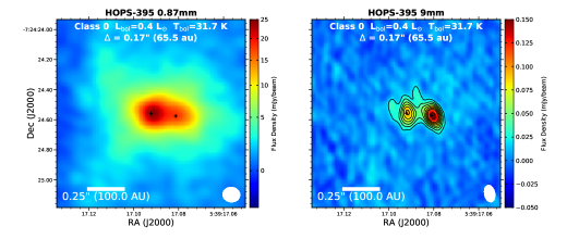
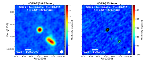
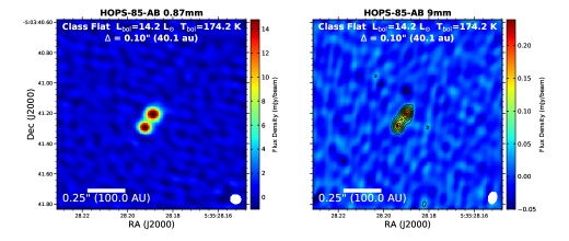
Figure 2: Examples of Class 0, Class I, and Flat Spectrum multiples from Orion; the ALMA images are shown on the left, and the VLA images are shown on the right. The Class 0 and Class I images are reproduced from Paper I, but the HOPS-85 images are produced with superuniform weighting (ALMA image, left) and robust=0 weighting (VLA image, right) showing the binary more clearly than the images from Paper I. HOPS-395 may have a shared inner disk or envelope surrounding the binary, the southern component of HOPS-323 appears to be an edge-on disk, and we only detect the individual circumstellar disks toward HOPS-85. The contours on the HOPS-85 VLA image start at $\pm$3$\sigma$ and increase by $\pm$2$\sigma$, where $\sigma$=11.3 $\mu$Jy/beam. Black crosses mark the source positions from the Gaussian fitting to the VLA data. The ALMA and VLA beam sizes are $\sim$0$\farcs$11 and $\sim$0$\farcs$08, respectively, while for HOPS-85 the respective beams are $\sim$0$\farcs$08 and 0$\farcs$06.

The Orion A and B molecular clouds provide the largest available sample of protostellar multiples with separations less than 500 au. We show example images for some close multiple systems with separations less than 500 au in Figure 2. At scales less than 100 au, most systems represent new discoveries.

We detect 19 Class 0 multiple systems with separations less than 500 au (17 binary, 2 triple); 10 Class I binary systems, 18 Flat Spectrum binary systems, and 3 additional binary systems that are not classified. Table The VLA/ALMA Nascent Disk and Multiplicity (VANDAM) Survey of Orion Protostars V. A Characterization of Protostellar Multiplicity lists all of these multiple systems. One of the unclassified systems resides in OMC1N (Teixeira et al., 2016) and is likely a protostar, but the other two are found toward systems with near-infrared counterparts detected by the 2MASS survey (Skrutskie et al., 2006) and are likely more evolved YSOs.

3.3 Close Multiples Not Detected By Both ALMA and VLA

The vast majority of multiple systems discovered in Orion were resolved and detected independently by ALMA and the VLA. However, there are a few examples where close multiplicity was detected only in the VLA observations or only in the ALMA observations. We also discuss examples where there is tentative evidence for a companion, but the evidence is not strong enough to merit inclusion in the sample of multiples.

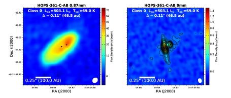
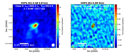
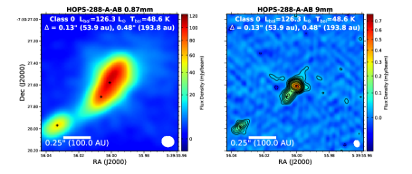
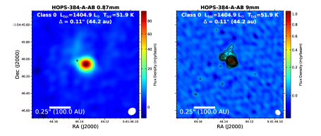
Figure 3: Multiple systems that are not detected by ALMA but are resolved by the VLA imaging. The lack of ALMA detections may be a combination of resolution and dust opacity. The VLA images are produced with robust=0 weighting. The contours start at 3$\sigma$, increase by 2$\sigma$ until 15$\sigma$, then increase by 5$\sigma$ until 30$\sigma$, and then increase by 10$\sigma$. The values for $\sigma$ are 10.8, 10.0, and 10.9 $\mu$Jy/beam for HOPS-361, HOPS-288, and HOPS-384, respectively. Black crosses mark the source positions from the Gaussian fitting to the VLA data. The ALMA and VLA beam sizes are $\sim$0$\farcs$11 and $\sim$0$\farcs$08, respectively.

HOPS-361-C (also known as NGC 2071 IRS3): Toward this protostar we detect two sources separated by $\sim$46.5 au (0$\farcs$108) only in the VLA 9 mm observations (Figure 3); the eastern source has a jet elongated nearly orthogonal to the position angle between the two components. The ALMA observations, on the other hand, detect only a large disk surrounding the two protostars, with some surface brightness variation. Extended emission from this disk is only visible at low S/N in the VLA data. It is unclear why the two protostars do not stand out within this disk, but the circumbinary disk could be optically thick at 0.87 mm, or the surface brightness of the circumbinary disk could be comparable to the intensity from the circumstellar disks around each protostar.

HOPS-361-E: This protostar also falls within the HOPS-361 region ($\sim$1140 au from HOPS-361-A) and only has its multiplicity detected by the VLA (Figure 3). This source was recognized as a multiple in further analysis of the NGC 2071 IR region by Cheng et al. (in prep.). Its separation of 0$\farcs$055 ($\sim$22 au) is too small to be resolved in our ALMA observations, and only the higher resolution afforded by the VLA observations enabled the system to be resolved. Thus, the compactness of this system resulted in it not being reported as a multiple in Paper I.

HOPS-288: We find another example of compact multiplicity toward this protostar, shown in Figure 3, where two continuum sources are clearly detected by both ALMA and the VLA and are separated by $\sim$220 au (0$\farcs$542). The brighter, western source is found to be extended in both ALMA and VLA images, but VLA imaging with higher resolution using a robust parameter of 0 (Briggs weighting) rather than Natural Weighting used in Paper I reveals that there are two point sources within the brighter source, separated by $\sim$54 au (0$\farcs$133). Imaging the ALMA data with lower values of the robust parameter to achieve higher resolution does not reveal the close companion source at 0.87 mm; this companion may also be obscured by optically thick continuum emission. This close companion is positioned along the expected axis of the disk of HOPS-288, orthogonal to the known molecular outflow from this protostar (Stanke et al., 2000; van Kempen et al., 2016).

HOPS-384: This is also a close multiple system that was only detected by the VLA (Figure 3). Similar to HOPS-288 and HOPS-361-C, HOPS-384 is also one of the highest luminosity HOPS protostars, as high as $\sim$1400 L_☉. The close companions are separated by 0$\farcs$11 in the VLA 9 mm image. The ALMA image at the highest resolution with superuniform weighting has a protuberance in the direction of the companion and detection may simply require higher resolution. There is a third companion to HOPS-384 located northwest by 3$\farcs$39 (not shown in Figure 3), but this source is not detected by the VLA and appears as a near edge-on disk in the ALMA 0.87 mm image (Tobin et al., 2020).

The next two sources are each in their own category. The first has companions detected by ALMA that were not subsequently detected by the VLA, and the second was not recognized as a separate protostellar system in Paper I, but is both a discrete protostellar system and a binary system.

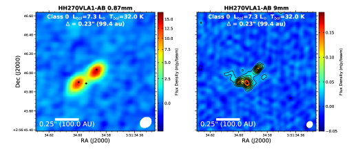
Figure 4: ALMA and VLA continuum images of multiples detected by VLA and ALMA, but not all sources are present at both wavelengths. Three sources of continuum emission are detected with ALMA for HOPS-56, but only two are detected by the VLA. All three are considered to be companions since the VLA is less sensitive to dust emission and the non-detection does not rule out one of the sources. For HH270VLA1 on the other hand, three sources are detected by the VLA and only 2 sources are detected by ALMA. The source not detected by ALMA is likely an outflow shock feature or a background AGN because of its strongly negative spectral index. The contours start at 3$\sigma$ and increase by 2$\sigma$ until 15$\sigma$, then increase by 5$\sigma$ until 30$\sigma$, and then increase by 10$\sigma$. The values for $\sigma$ are 8.1 and 8.5 $\mu$Jy/beam for HH270VLA1 and HOPS-56, respectively. The black crosses mark the source positions from Gaussian fitting to the VLA data for HH270VLA1 and the ALMA data for HOPS-56. The ALMA and VLA beam sizes for HH270VLA1 are $\sim$0$\farcs$11 and $\sim$0$\farcs$06, respectively, and for HOPS-56 the respective beam sizes are $\sim$0$\farcs$11 and $\sim$0$\farcs$08.

HOPS-56 has companions detected by ALMA but not by the VLA. It is detected as a close triple system in the ALMA image (Figure 4), both companions having separations of $\sim$0$\farcs$22. However, the VLA image toward HOPS-56 does not detect all three components, failing to detect HOPS-56-A-B, likely due to poorer dust mass sensitivity in the VLA data as compared to ALMA. Given the high-confidence detection of all three sources with ALMA, we consider all three of these sources as companions.

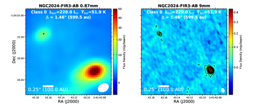
Figure 5: ALMA (left) and VLA (right) continuum images of the Class 0 system NGC 2024 FIR 3. The ALMA image was not observed by our program, but is an ALMA 1.3 mm image from van Terwisga et al. (2020). The contours start at 3$\sigma$ and increase by 2$\sigma$ until 15$\sigma$, then increasing by 5$\sigma$ until 30$\sigma$, and then increasing by 10$\sigma$. The value for $\sigma$ is 8.5 $\mu$Jy/beam. The black crosses mark the source positions from Gaussian fitting to the VLA data. The ALMA beam is $\sim$0$\farcs$25, and the VLA beam is $\sim$0$\farcs$08.

NGC 2024 FIR-3 was added to the sample in subsequent analysis of the data since the publication of Paper I. This source was detected in the VLA data toward HOPS-384 presented in Paper I, but it was not identified as a multiple system there because its nature was uncertain, and there were no ALMA data covering that region in our survey. An ALMA survey of the region by van Terwisga et al. (2020) associated the continuum at 1.3 mm emission with NGC 2024 FIR3, which was classified as a Class 0 system by Ren & Li (2016) with a bolometric luminosity of 220 L_☉. Given the association with a bonafide protostar system, we include this detection in our multiplicity statistics with a separation of 1$\farcs$46 ($\sim$586 au) and show the ALMA 1.3 mm image from van Terwisga et al. (2020) and the VLA images in Figure 5. While we zoom-in more closely on the source, the wider field image from van Terwisga et al. (2020) shows significant extended structure associated with the envelope.

The following three protostars have possible companions where tentative evidence is found in the VLA data but not the ALMA data. We do not include these companions in our multiplicity statistics given their tentative nature.

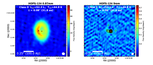
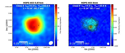
Figure 6: ALMA and VLA continuum images of possible multiples detected in VLA imaging but not in the ALMA imaging. These are classified as possible multiples due to the low amplitude of their peak intensity above the noise, so they are not included in the multiplicity statistics. In the case of HOPS-124 (top row), the possible companion is also detected in the outflow direction, corresponding to the near center of the crescent-shaped dust emission from the ALMA image. The ALMA HOPS-124 image is produced with superuniform weighting, while the VLA image is produced with robust=-1 and only for the 8.1 mm portion (the highest frequency half of the VLA data) of the data. The 0.87 mm continuum emission for HOPS-403 is likely optically thick (Karnath et al., 2020), which is probably the reason for the lack of detection toward the two peaks by ALMA. In the VLA images, the contours start at 3$\sigma$, increase by 2$\sigma$ until 15$\sigma$, then increase by 5$\sigma$ until 30$\sigma$, and then increase by 10$\sigma$. The values for $\sigma$ are 6 and 24 $\mu$Jy/beam for HOPS-403 and HOPS-124, respectively. The black crosses mark the source positions from Gaussian fitting to the VLA data. The ALMA and VLA beam sizes for HOPS-124 are $\sim$0$\farcs$09 and $\sim$0$\farcs$06, respectively, and for HOPS-403 the respective beam sizes are $\sim$0$\farcs$11 and $\sim$0$\farcs$07.

HOPS-124: This is a Class 0 protostar with a large disk that has asymmetric dust emission with an apparent gap (Sheehan et al., 2020). An obvious culprit that can produce such features is a companion star that formed within the disk. Images produced with Robust=-1 of only the highest frequency half of the VLA 9 mm dataset ($\lambda\sim$8.1 mm) detect a possible second source separated by $\sim$0$\farcs$08 (Figure 6). However, this possible second source is along the direction of the outflow and could be part of the jet since extended free-free emission associated with the jet is seen in Ka-band toward some sources (see Figure 3). We are therefore hesitant to claim this as a companion since it could also be an extension of the compact jet emission. This possible second source is also coincident with the bright dust ring that appears in the ALMA images and the VLA image produced with robust=2 weighting (Paper I; Sheehan et al., 2020). Therefore, this second source could instead be a clump of dust in the disk and not a true companion. Consequently, this possible source is not included in our multiplicity statistics.

HOPS-403: This is an extended source in both 0.87 mm and 9 mm dust continuum emission (Figure 6). This protostar is a member of a subset of the Class 0 protostars that are more deeply embedded than typical Class 0 protostars and may be one of the youngest protostars in Orion, which are known as PACS Bright Red Sources (PBRS; Stutz et al., 2013; Tobin et al., 2015; Karnath et al., 2020). The ALMA 0.87 mm image only shows a fairly smooth surface brightness distribution with a $\sim$1″ diameter, while VLA 9 mm data reveal further sub-structure, including a possible second point source with a separation of $\sim$0$\farcs$15, located west of the brighter source. However, its contrast with respect to the surrounding continuum emission is only $\sim$3$\sigma$. There is no evidence for this second source in the ALMA 0.87 mm data due to the optical depth of the continuum (Karnath et al., 2020). Thus, we are hesitant to definitively claim that this is a companion, and this source is not included in our multiplicity statistics.

HH270VLA1: Toward this Class 0 protostar, both VLA and ALMA detect two components separated by 0$\farcs$23 (Figure 4). However, there is a third component detected by the VLA at Ka-band. This third source has a radio spectral index of $\sim$-0.4, indicating non-thermal emission. Thus, this third source is either a shock in the outflow, similar to the extended jets observed toward HOPS-370 (Tobin et al., 2019; Osorio et al., 2017) and HOPS-361-C (Figure 3; (Carrasco-González et al., 2012, Cheng et al. in prep.)), or it is a background active galactic nucleus (AGN). The probability of a background AGN aligning so closely with a binary protostar is very small, $\sim$10^-5, see Tobin et al. (2016a). For this reason, we do not consider the third source, denoted HH270VLA1-C in Paper I, a companion.

3.4 Impact of Non-detections or Spurious Detections

Given that the total sample size is $\sim$300 protostars for Orion, and there are $\sim$100 in each protostellar class, the inclusion or exclusion of any particular source will impact the resulting MFs and CFs by $\pm$0.01. With the typical uncertainties of 0.03 to 0.05, we would have over or under count by $\sim$6 to 10 sources to end up with multiplicity statistics that are inconsistent by $>$1$\sigma$. Either way, if there are undetected companions by either ALMA or the VLA (see Section 3.6) or the seven possible transition disks detected by Sheehan et al. (2020) are really circumbinary disks, the statistics will be further underestimated.

3.5 Dynamic Range of Detected Systems

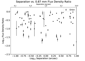
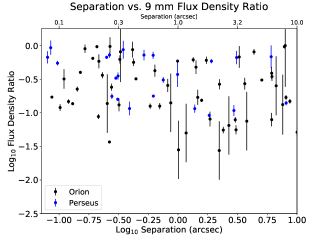
Figure 7: Flux density ratio versus separation for the companions observed at 0.87 mm (left) and 9 mm (right). It is not clear if there is an intrinsic contrast limit at smaller separations, and the contrast limits may be limited by the physical disk structures within an individual system, in addition to instrumental dynamic range limits. The uncertainties here are statistical only and do not include absolute flux calibration uncertainty. However, the vast majority of points plotted are within the same field of view and would not have absolute calibration that is systematically different.

We examined the companion flux density ratios as a function of separation in Figure 7. The flux density ratios are shown in separate panels for the ALMA 0.87 mm and VLA 9 mm. Tables The VLA/ALMA Nascent Disk and Multiplicity (VANDAM) Survey of Orion Protostars V. A Characterization of Protostellar Multiplicity and The VLA/ALMA Nascent Disk and Multiplicity (VANDAM) Survey of Orion Protostars V. A Characterization of Protostellar Multiplicity list the ratios corresponding to each system, but we only provide the ratios for individual source pairs and not when a source is paired with an existing multiple or when two multiple systems are joined. We find that there is no clear contrast limit for the detection of companions that is progressively lower as separation decreases. The majority of companions tend to have flux density ratios that are within a factor of 10. Only a few have ratios greater than a factor of 100, and those are only seen in the ALMA data for companions that have separations approaching 10″. Thus, it is not clear if dynamic range limits affect our ability to detect multiplicity in protostars with the current data. There are also additional factors to consider since we are detecting emission from extended dusty disks rather than stellar point sources. Source separation plays a role in defining the extent of their circumstellar disks (Artymowicz & Lubow, 1994). Then, the flux density that we observe is determined from a combination of dust mass and disk radial size (or simply surface density), both of which are related to the dust continuum opacity.

These flux density ratios have no relation to the underlying mass ratios of these systems because there are clear examples where the brightest dust continuum source in a system is not the most massive (e.g., L1448 IRS3B; Tobin et al., 2016b; Reynolds et al., 2021). The ratios could be interpreted as a dust mass ratio of the circumstellar disks around each component of a multiple system, with the caveat that the VLA data can have contributions from free-free emission. However, such comparisons can be misleading if a substantial amount of the dust is optically thick. We avoid over-interpreting the flux ratios, but provide them as a observational characteristic of the systems.

3.6 Near-infrared vs. ALMA/VLA Detections

The large sample of HOPS protostars observed with HST NICMOS and WFC3 (Kounkel et al., 2016; Habel et al., 2021) enables us to compare protostellar multiples that are detected from their direct stellar emission to those detected via their circumstellar dust emission. This allows us to determine how much incompleteness there might be in a particular type of observation. For the purposes of this analysis, we only consider multiples that would have been within the range of detection by both projects, which limits the analysis to separations between $10^{2}$ and $10^{3}$ au ($\sim$0$\farcs$25 to $\sim$2$\farcs$5). We emphasize that even if a companion is detected by HST and not ALMA/VLA, we do not add it back into our current analysis, leaving our analysis based on ALMA/VLA data alone.

There were a total of 274 HOPS protostars observed by both ALMA/VLA and HST at 1.6 $\mu$m Kounkel et al. (2016). Neither ALMA/VLA nor HST detect companions toward 235 protostars, both ALMA/VLA and HST detect the same companions toward 19 protostars (2 Class 0; 6 Class I, and 11 Flat Spectrum), ALMA/VLA alone detects a companion toward 12 (9 Class 0 and 3 Class I) protostars, and HST alone detects a companion toward 8 (4 Class I, and 4 Flat Spectrum) protostars. We consider four of the HST-only companions as tentative given that they are very faint (HOPS-5, HOPS-65, HOPS-86, and HOPS-281); HOPS-281 is also a tentative companion for the ALMA detection.

Between $10^{2}$ and $10^{3}$ au, we estimate a submillimeter/centimeter incompleteness of $\sim$20% (as given by 1-[Number of detected companions/Total companions]; Total companions is the millimeter plus infrared companions). Considering only Class I and Flat Spectrum protostars, the incompleteness rises to 29%. The infrared-only incompleteness is 31% if Class 0 protostars are included in the counting, but drops to $\sim$11% if only Class I and Flat spectrum protostars are included. Much of this incompleteness in the infrared is due to extinction; Class 0 protostars are rarely detected in the HST 1.6 $\mu$m data, while many Class Is are only detected in scattered light (Habel et al., 2021). The detection of companions in the HST data is primarily toward the $\sim$30% of the protostars that are visible as point sources (Kounkel et al., 2016). Thus, both techniques may have comparable levels of incompleteness depending on the class of protostar observed. However, submillimeter/millimeter observations are clearly superior for characterizing Class 0 multiplicity, while near-infrared observations appear superior for characterizing Class I and Flat Spectrum multiplicity at separations $>$100 au. On the other hand, separations $<$100 au may be problematic in the near-infrared for Class I protostars with significant envelopes due to significant scattered light confusion and dust opacity. Infrared observations at $<$100 au separations may be most effective for the more evolved Flat Spectrum protostars.

A weakness of the near-infrared observations is that they also have a greater likelihood of contamination as compared to submillimeter and millimeter observations. This is because contamination can come from foreground or background stars, and contamination becomes extremely problematic at projected separations $>10^{3}$ au (Kounkel et al., 2016). Submillimeter and millimeter observations are also susceptible to contamination, as described in Appendix A, but the requirement for them to have either dusty emission or free-free emission significantly reduces the number of possible contaminating sources relative to near-infrared.

4 Overall Multiplicity Characterization

We describe the overall multiplicity results from our observations in the following subsections. The Orion results are the main focus, but we also include details of Perseus where relevant and when the results are distinct from those of Tobin et al. (2016a).

4.1 Bolometric Luminosities and Temperatures

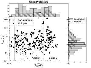
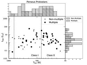
Figure 8: Bolometric temperature vs. bolometric luminosity plots for both Orion and Perseus. Single systems are represented by small points, while the large points represent the composite luminosity of each multiple system, with separations up to 10⁴ au. Histograms are shown along the top and right axes for the scatter plots along those directions. It is apparent that the T_bol distributions are quite similar for singles vs. multiple systems, while the luminosity distributions appear different. For Orion the median luminosities of single and multiple systems are 0.96 and 3.27 L_☉, respectively, and for Perseus the median luminosities for single and multiples systems are 0.97 and 3.06 L_☉, respectively. The difference between the two distributions (singles vs. multiples) is statistically significant for Orion, while for Perseus the difference is not quite statistically significant (see Section 4.1).

We start by examining T_bol vs. L_bol for the single systems vs. the multiple systems as shown in Figure 8. The figure shows all systems that are multiple from 20 to 10000 au. It is apparent that the luminosities of multiple systems, which implicitly includes the luminosities of all protostellar members, are systematically higher than the luminosities of systems that are single at our resolution limit. The median luminosities for singles and multiples in Orion are 0.96 and 3.27 L_☉, respectively, and for Perseus they are 0.97 and 3.06 L_☉, respectively. The difference is quite obvious in Orion and is also discernible by-eye in Perseus, despite a smaller sample size. We compared the L_bol distributions for single vs. multiples using the KS-test, and for Orion the null hypothesis that singles and multiples are drawn from the same parent distribution is ruled out with a likelihood of $<$ 0.01; the null hypothesis cannot be ruled-out at the same likelihood level for Perseus, where we find a likelihood of 0.025. For both Perseus and Orion, the T_bol distributions are consistent with having been drawn from the same sample. We further note that the median luminosity differences and inconsistency of the luminosity distributions persist for different separation ranges (20 to 500 au and 20 to 10³ au, in addition to the shown range of 20 to 10⁴ au).

The skew toward higher luminosities for the multiples could be related to the fact that multiple systems occur more frequently for higher-mass systems (e.g., Duchêne & Kraus, 2013). However, this is speculative given that the protostellar masses are not known for the majority of these multiple systems. But, in any event, two (or more) protostars accreting at similar rates will naturally have a higher luminosity than a single protostar accreting at the same rate.

4.2 Separation Distributions

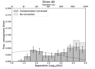
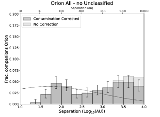
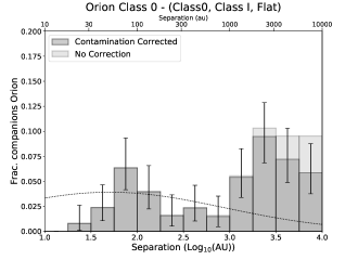
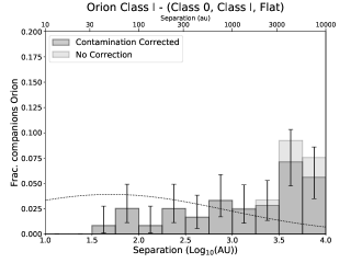
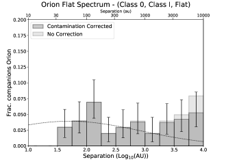
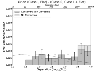
Figure 9: Histograms of companion separations for different selections from the Orion sample. The histograms specifying a particular protostar class only include separations from each protostar to the specified class. Separations that include protostars from different classes or more than one unclassified source are only shown in the panel labeled ‘All’. The lighter gray histograms do not include the companion probabilities as determined from the YSO surface density. This shows that contamination is likely only significant for separations greater than 3000 au. The thin dotted curve in each panel is the Gaussian fit to the separation distribution of solar-type field stars (Raghavan et al., 2010). The resolution limit for Orion and Perseus is $\sim$20 au (1.3 in log units). The error bars for each bin are computed using binomial statistics as discussed in Section 2.4.3. The number of separations contributing to each bin are then divided by the total number of singles and the total number of separations displayed in the plot.

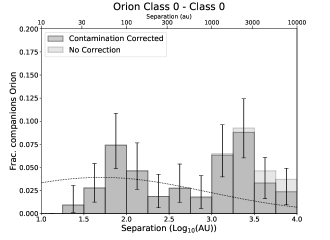
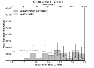
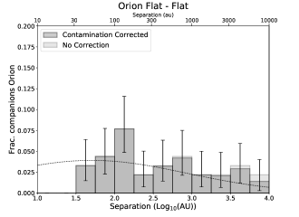
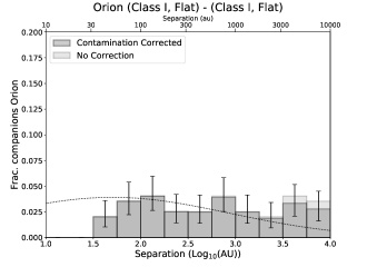
Figure 10: Same as Figure 9, but for histograms constructed only for protostars of the same class within Orion.

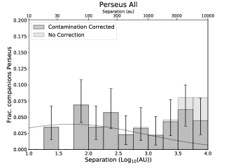
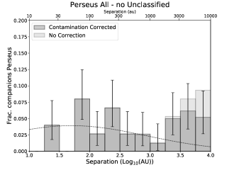
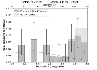
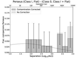
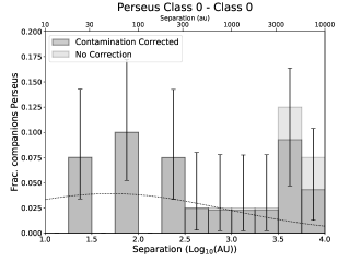
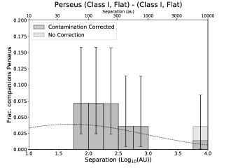
Figure 11: Same as Figure 9 but for Perseus.

A major goal of this study is to better determine the typical separations of companion stars, which can be connected to formation mechanism. We use the list of all separations measured (Tables The VLA/ALMA Nascent Disk and Multiplicity (VANDAM) Survey of Orion Protostars V. A Characterization of Protostellar Multiplicity and The VLA/ALMA Nascent Disk and Multiplicity (VANDAM) Survey of Orion Protostars V. A Characterization of Protostellar Multiplicity) following the analysis methods described in Section 2.4 and Appendix A to generate histograms and cumulative distributions for companion stars in different separation bins. These histograms are generated with bin sizes of 0.25 for the log₁₀ of the projected separation in au. The separation distribution histograms of the Orion results for the full sample, Class 0 protostars, Class I protostars, Flat Spectrum protostars, and Class I and Flat Spectrum protostars considered together are shown in Figure 9 . We then show the Orion separation distributions limited to only protostar separations of a particular class in Figure 10. Finally, the separation distributions for Perseus are shown in Figure 11. In this and the following sections, and in Tables 5 Orion and Perseus Multiplicity and Companion Fractions with Probabilities, 6 Combined Multiplicity and Companion Fractions with Probabilities, and 7 Multiplicity and Companion Fractions at High and Low YSO Surface Densities, we refer to the different multiple systems of protostars from different classes in the following manner, with the first class listed representing the majority classification of the system and the second item refers to the classes of the other system components. We use the following classifications:

• Class 0–Class 0,

• Class 0–(Class 0, Class I, Flat),

• Class I–Class I,

• Class I–(Class 0, Class I, Flat),

• (Class I, Flat)–(Class I, Flat),

• (Class I, Flat)–(Class 0, Class I, Flat),

• Flat–Flat

• Flat–(Class 0, Class I, Flat).

For example, Class 0–Class 0 specifically refers to multiple systems that are only composed of Class 0 protostars. These could be binaries, triples, or higher order, but all have the Class 0 classification. Then, Class 0–(Class 0, Class I, Flat) will include multiple systems that include protostars of all Classes and not just Class 0s; however, the primary classification of the system will be Class 0 due to a majority of its components being Class 0 (see Appendix A.3). This categorization does not result in double counting of multiples between systems that are composed of different Classes, but Class 0–Class 0 and Class 0–(Class 0, Class I, Flat) do overlap in their samples. However, one can see some differences visually in Figures 9 and 10 between homogeneously classified multiples and multiples with composite classification.

We note that some composite categories, like (Class I, Flat)–(Class I, Flat), are needed because the available Perseus classifications did not distinguish between Class I and the more evolved Flat Spectrum protostars. Thus, to compare with Orion, it is more appropriate to consider the composite category.

The histograms generated for the Orion protostars fill the range of parameter space from 20 au to $10^{4}$ au. The histogram for the full sample (see Figure 9) shows some structure with a peak at $\sim$75 au and another peak at $\sim$4000 au. Multiples exist between these two peaks, but there is a local minimum that is visually apparent at $\sim$300 au, and the histogram does not begin rising again until separations $\geq$10³ au. We note that the scheme for determining the probability of a detected continuum source to be a companion (Section 2.4.3) lowers the significance of the peak at large separations but does not affect the histograms significantly at less than $\sim$3000 au. The separation histograms for Perseus appear similar to those of Orion (Figure 11), with most of the histogram bins being within their 1$\sigma$ uncertainties.

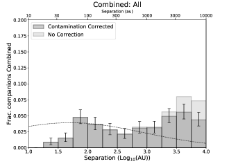
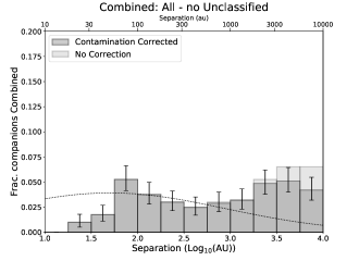
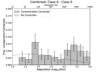
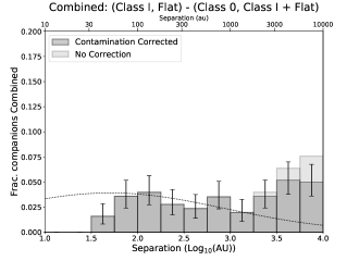
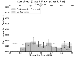
Figure 12: Same as Figure 9 and 11 but for histograms constructed from the combined sample of Orion and Perseus. Class I and Flat Spectrum are not differentiated here because the Perseus sample does not distinguish between Flat Spectrum and Class I sources.

The separation distributions for Class 0 protostars (for both homogeneous and composite systems) appear the most distinct relative to the separation distributions of Class I and Flat Spectrum protostars. The principal difference is the bimodal appearance of the Class 0 distributions, while the separation distributions of more evolved systems tend to be more flat and exhibit less structure. Thus, it is the Class 0 protostars that are primarily responsible for this bimodal appearance in the full sample (Figures 9 and 10). Because the trends in both regions are similar, we are motivated to combine the datasets to improve the statistics of the separation distributions. We show the separation distribution histograms for the combined Orion and Perseus samples in Figure 12. The combination of the samples results in a smoother distribution of separations due to the greater numbers, but is not fundamentally different from Orion and Perseus on their own.

4.3 Quantitative Separation Distribution Comparisons

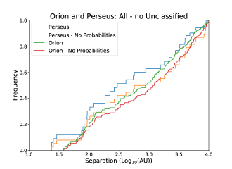
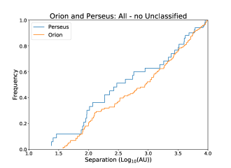
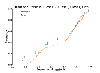
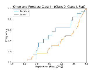
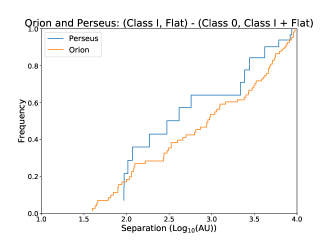
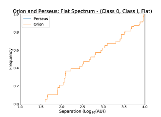
Figure 13: Cumulative separation distributions for Orion and Perseus protostars for different protostar classes. The samples for different protostar classes are all consistent with being drawn from the same parent distribution. The upper left panel shows the impact of our companion probabilities on the CDFs for the full sample.

The distributions of separations, as shown in the histograms in Figures 9, 10, 11, and 12, are illuminating, but they do not quantitatively demonstrate whether or not Perseus and Orion are statistically different or if analytic distributions are consistent with the observations. Statistical tests are necessary to determine if the observed populations are likely drawn from the same parent distribution. To evaluate this, we constructed (CDFs) from the separation distributions and used their respective companion probabilities to compare the distributions by randomly sampling the separation distribution CDFs 1000 times and comparing each of these randomly sampled CDFs using the KS test as described in the Appendix A.2. We only considered the full separation range (20 to 10⁴ au), because the separation distributions from 20 to 10³ au could not rule out the null hypothesis for any tests. Figure 13 shows the CDFs for Orion and Perseus; the upper left panel shows the effect of the companion probabilities on the CDFs for the full sample.

4.3.1 Orion and Perseus Comparisons

We first compared the Orion and Perseus separation distributions or all possible combinations of the same classes. The median likelihoods and their uncertainty (defined by quartiles) for the randomly sampled CDFs are used to evaluate the statistical tests. We find that the null hypothesis cannot be ruled out for any of the Orion and Perseus separation distributions, meaning that there is no statistical evidence for the Perseus and Orion separation distributions to be drawn from different samples. The sample with the lowest median likelihoods were Class I–Class I and (Class I, Flat)–(Class I, Flat).

4.3.2 Comparison Between Classes

In Section 4.2, we highlighted some visual differences between the separation distributions of different Orion protostar Classes. Here we now evaluate whether they are statistically significant. Out of all the classes, only comparisons between Class 0–(Class 0, Class I, Flat) vs. Flat–Flat and Class I–(Class 0, Class I, Flat) vs. Flat–Flat had median likelihoods that were $<$0.01 along with more than half of their realizations having likelihoods $<$ 0.01. One other comparison, Class 0–Class 0 vs. Class I–(Class0, Class I, Flat) nearly made the cutoff for a statistically significant difference with a median likelihood of 0.011. Thus, the most significant difference in separation distribution can be observed between the youngest multiple systems and the most-evolved multiple systems in Orion. The principal difference in the histograms shown in Figures 9 and 10 is that the Class 0–(Class 0, Class I, Flat) distribution has significantly more companions at separations $>$1000 au as compared to the Flat–Flat distribution.

We also compared the separation distributions of the combined Orion and Perseus samples. In this comparison we only find a statistically significant difference for Class 0–(Class 0, Class I, Flat) vs. (Class I, Flat)–(Class I, Flat), with a median likelihood of 0.002. Like the results from Orion only, we find a statistically significant difference between the youngest systems and those that are the most evolved.

4.3.3 Comparison with a Log-Flat Distribution

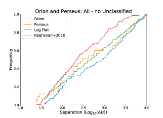
Figure 14: Cumulative separation distributions for Orion and Perseus protostars shown relative to a log-flat separation distribution and the separation distribution for solar-type field stars from (Raghavan et al., 2010). The log-flat distribution shown is calculated with respect to the Orion separations.

We also compared our separation distribution to an analytic distribution that is flat in $log$ separation space, a log-flat distribution, which is commonly referred to as Öpik’s law (Öpik, 1924) and has been found to describe populations of companion separations (e.g., Kouwenhoven et al., 2007). We show an example log-flat separation distribution in Figure 14. Comparing with a log-flat distribution also indirectly checks whether the bimodal appearance is statistically robust. We performed a one-sided KS-test with an analytic log-flat distribution. The results from 1000 KS-tests, sampling the source separation distribution according to the probabilities are comparable to using a 2-sample KS-test with a log-flat distribution with a sample size 100$\times$ the size of the input sample. Only the Orion Class 0–(Class 0, Class I, Flat) sample and the Class I–(Class 0, Class I, Flat) sample were able to reject the null hypothesis with a median likelihood $<$ 0.01.

The Perseus separation distributions were also tested against a log-flat separation distribution, but none of the Perseus sub-samples nor overall sample are able to reject the log-flat separation distribution with a likelihood $<$ 0.01. This is contrary to the result from Tobin et al. (2016a) which found evidence that a log-flat distribution could be ruled-out for the full sample, with a likelihood $<$ 0.1. However, in this study none of the Perseus samples are able to rule-out the null hypothesis even for likelihoods of 0.1. The sample that has the lowest likelihood is the Perseus Class 0–(Class 0, Class I, Flat) sample with a likelihood of 0.11. To investigate if our companion probability scheme is the cause of the difference, we also performed the comparison with a distribution of separations without probabilities (assuming all are companions), and the lowest likelihood was 0.135, also for Class 0–(Class 0, Class I, Flat) (see Appendix B). The reason why we do not find the same result as the previous study is because the separation distributions are constructed differently and use automated methods rather than manual associations. In this case, the main source of difference arises from the higher order systems whereas the previous study chose the primary and separations were all calculated with respect to the primary.

We also compared the combined sample of Orion and Perseus with the log-flat distribution. Similar to the case for Orion alone, both Class 0–(Class 0, Class I, Flat) and Class I–(Class 0, Class I, Flat) samples are able to reject a log-flat distribution, having median likelihoods $<$ 0.01. Ruling-out this commonly observed distribution of separations provides evidence that the structure in those separation distributions is real and is not the result of statistical uncertainty or histogram binning. In particular, for the Class 0–(Class 0, Class I, Flat) distribution, ruling-out the log-flat distribution suggests that the bimodal appearance may be real.

4.3.4 Comparison Field Solar-type Multiples

We next compared the observed separation distributions to the distribution of separations for field solar-type stars (Raghavan et al., 2010) using the KS test. We make use of the observed separation distribution from 24 to 10⁴ au from Raghavan et al. (2010), sampling the same range of separations for which we have detections. We show the distribution from Raghavan et al. (2010) along with the observations of the cumulative distribution for the full samples for Orion and Perseus in Figure 14. While the field solar-type stars are a well-characterized sample to compare with, it is important to highlight that most of the protostars in the HOPS sample are likely to become M-stars rather than F, G, or K-type stars that make up the Raghavan et al. (2010) sample.

For Perseus alone, we can only reject the null hypothesis for the Class 0–(Class 0, Class I, Flat) sample. Then, for Orion, the null hypothesis is ruled out for all Classes except for the Flat–Flat, Flat–(Class 0, Class I, Flat), and Class I–Class I samples. Only the separation distributions for the more evolved protostars in Orion cannot be distinguished from the separation distribution of field solar-type stars. The comparison of the Raghavan et al. (2010) distribution to the combined Orion and Perseus samples yields similar results to those for Orion alone.

4.4 Overall Multiplicity Statistics

We compute the MFs and CFs for the protostars in Orion, Perseus, and their combined sample. The statistics are examined for a variety of separation ranges to both illustrate the size scale on which most multiples are found and evaluate whether there are differences between classes for the different separation ranges. The MFs and CFs for Orion, Perseus, and their combined samples are provided in Tables 5 Orion and Perseus Multiplicity and Companion Fractions with Probabilities and 6 Combined Multiplicity and Companion Fractions with Probabilities and will contain information related to the formation mechanism(s) and the evolutionary paths of multiplicity.

The Orion and Perseus samples on scales from 20 au to 10⁴ au have MFs of 0.30$\pm$0.03 and 0.38$\pm$0.07, respectively. The respective CFs are then 0.44$\pm$0.03 and 0.57$\pm$0.07. For the separation range from 20 au to 10³ au, the MFs drop to 0.17$\pm$0.02 and 0.26${}^{+0.06}_{-0.05}$, and the CFs drop to 0.19$\pm$0.02 and 0.28$\pm$0.06, respectively. This shows numerically that about 1/3 of the multiples in Orion and Perseus are found at 10³ to 10⁴ au separations. The CFs are nearly identical to the MFs on 20 au to 10³ au scales because there are few triples and high-order multiples detected on these smaller scales. The MFs and CFs for the full samples of protostars in Orion and Perseus are consistent within their uncertainties. The MFs and CFs computed here for Perseus are lower than previously presented in Tobin et al. (2016a). These differences are largest for the MFs and CFs computed using the companion probabilities but are still present even if the companion probabilities are not taken into account (see Appendix A.5). Thus, the differences result from both the companion probabilities and our new method for associating multiples.

The typical architectures of the multiple systems are also found in Tables 5 Orion and Perseus Multiplicity and Companion Fractions with Probabilities and 6 Combined Multiplicity and Companion Fractions with Probabilities, where the number of systems that correspond to binaries, triples, quadruples, etc. is provided. For separations from 20 to 500 au and 20 to 1000 au, the most common architecture is binaries, outnumbering triples by a factor of $\sim$20 for separations between 20 and 500 au, and a factor of $\sim$15 for separations between 20 and 1000 au. Binaries are still the most common type of multiple system for separations between 20 and 10⁴ au, but the ratio of binaries to higher order systems is now only a factor of $\sim$4. In fact, some systems that were binaries at smaller separation ranges are part of higher-order systems when larger separations are considered. Systems higher order than triple are relatively uncommon and the number of triples found within the separation range between 20 and 10⁴ au, is comparable to the total number of all systems with 4 or more components. However, in Orion, the total number of individual components within quadruples or higher-order systems (44) is larger than the number of individual components in triples (27).

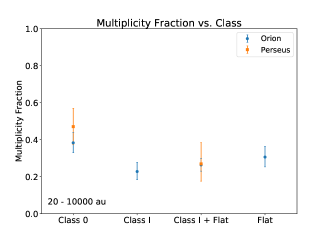
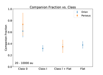
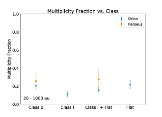
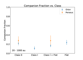
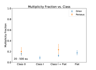
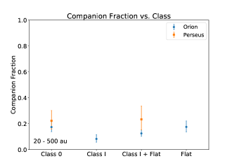
Figure 15: Plots of Multiplicity Fraction (left) and Companion Fraction (right) for different ranges of separations and plotted as a function of protostellar class for Orion and Perseus. The CFs on 20 to 10⁴ au scales for Class 0 protostars differ by $\geq$2$\sigma$, but less than 3$\sigma$, with respect the other Classes.

We plot the MFs and CFs as a function of protostellar class in Figure 15 for Orion and Perseus in three separation ranges: 20 to 10⁴ au, 20 to 10³ au, and 20 to 500 au. On the 20 to 10⁴ au range, the MFs and CFs for Class 0s are systematically higher than those for Class Is and Flat Spectrum protostars, similar to the results from previous studies (e.g., Chen et al., 2013; Tobin et al., 2016a). However, only the differences in the CF approach statistical significance in the separation range of 20 to 10⁴ au: 2.7$\sigma$ for Class 0s relative to Class I and 2.8$\sigma$ for Class 0s relative Class I and Flat Spectrum protostars. Then the difference is 2$\sigma$ for Class 0 to Flat Spectrum protostars, while the differences in the MFs and CFs between other classes are not statistically significant. This tells us that there are more higher-order companions to Class 0 protostars than more evolved protostars when separations out to 10⁴ au are considered. Our observed CFs for Class 0s are similar to those reported in Chen et al. (2013), but our MFs for Class 0 protostars are $\sim$30% lower than Chen et al. (2013). We suspect that this is due to sample bias in Chen et al. (2013), given that some of the archival data studied were previously known to be multiple systems and our larger samples are balanced both by detection of new multiples and also non-multiples.

The MFs and CFs computed in the 20 to 10³ au and 20 to 500 au ranges tell a somewhat different story. The overall MFs and CFs for both Perseus and Orion decrease, in part because continuum sources that are part of a multiple system at separations out to 10⁴ au are considered as independent, single sources for the 500 and 10³ au statistics. This increases the number of singles counted overall and for each class, resulting in a reduced MF and CF. Even if we did not count the singles in this way, the MFs and CFs would still decrease due to fewer multiples and higher-order multiples on these scales.

The overall trend in the MFs and CFs may show that multiplicity decreases from Class 0 to Class I and then rises from Class I to Flat Spectrum. However, this apparent trend is not statistically robust with the data in hand given that neither the MFs nor CFs have differences $>$3$\sigma$.

The differences in the CFs for Class 0 protostars with respect to Class I and Flat Spectrum protostars result from there being more companions at $>$1000 au toward Class 0 protostars than the Class I and Flat Spectrum protostars. The separation distributions of Class 0 protostars relative to Class I and Flat Spectrum protostars also show large differences at $>$1000 au, and some of the Class 0 separation distributions are statistically inconsistent with the distributions of more-evolved classes, see Section 4.3.2. These results imply that the principal change in multiplicity with protostellar evolution primarily affects companions with separations between 10³ and 10⁴ au because the MFs and CFs are comparable for Class 0 and Flat Spectrum protostars in the 20 to 10³ au and 20 to 500 au ranges.

The sizes of the Class I and Flat Spectrum samples in Orion are similar; thus, there is no clear sample bias that would produce a difference in the multiplicity statistics between Class 0 and more-evolved protostars. Flat Spectrum protostars are drawn from a parameter space that overlaps Class I protostars in terms of T_bol. The Orion Flat spectrum protostars have T_bol values that are skewed toward larger values of T_bol than typical Class I protostars (Paper I). Such a signature could not be searched for in Perseus due to a lack of necessary mid-infrared spectroscopy data from Spitzer toward the Perseus protostars as compared to the Orion protostars.

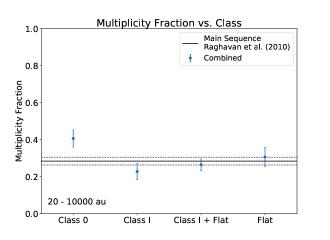
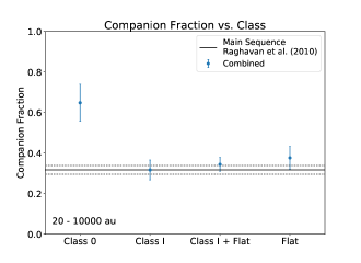
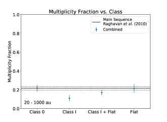
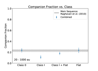
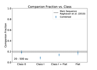
Figure 16: Same as Figure 15 but for the combined sample of Orion and Perseus. The MF and CF for solar-type field stars from Raghavan et al. (2010), calculated for the same ranges of separations as the protostar data, are also included for comparison. The Class 0 protostars are inconsistent with field stars for separations of 20 to 10⁴ au but are consistent for separations of 20 to 10³ au and 20 to 500 au. The most evolved protostars (Flat Spectrum) are consistent with the field at all ranges of separations.

We also examine the MFs and CFs for Orion and Perseus as a combined sample as a function of protostellar class and different ranges of separations in Figure 16. However, due to the lack of distinction between Class I and Flat spectrum in Perseus, the combined sample is only relevant for the full sample, Class 0, and Class I + Flat Spectrum samples. For Class I and Flat Spectrum, the combined statistics simply use those from Orion. Using the data from Raghavan et al. (2010), we calculate the field star MFs and CFs for system separations of 20 to 10⁴ au (0.28$\pm$0.02 and 0.32$\pm$0.02, respectively), 20 to 10³ au (0.22$\pm$0.02 and 0.23$\pm$0.02), and 20 to 500 au (0.19$\pm$0.02 and 0.20$\pm$0.02).

The MFs and CFs for the Class 0 and Flat Spectrum protostars for separations between 20 and 10³ au and 20 to 500 au are consistent with the field solar type stars. The Class I protostars have MF and CF values below that of the field solar-type stars within these two ranges of separations, but the differences are $<$ 2$\sigma$ for the 20 to 500 au separation range and are $\sim$2.3$\sigma$ for the 20 to 1000 au separation range. The Class I + Flat sample is also lower than that of the field stars but is consistent within the 2$\sigma$ uncertainties. At separations from 20 to 10⁴ au, only the Class 0 MF and CF disagree with those of solar-type field stars; the MF, however, has differences $<$2$\sigma$ but the CF difference is greater than 4.6$\sigma$. The higher multiplicity statistics of Class 0 protostars indicate both that stars form with higher multiplicity and that this early multiplicity also tends to comprise higher order systems. Based on the comparison of the MFs, CFs, and separation distributions in Section 4.3.3, the multiplicity properties of more evolved protostars tend to be the most similar to the field solar-type stars, and the Class 0 multiples tend to be the most dissimilar from those of field stars. We do note, however, that it is expected that most of the protostars studied in this work will not become solar-type stars based on the expected initial mass function.

4.5 Relationship Between Multiplicity and YSO Density

Previous multiplicity studies have examined the relationship between MF/CF and the local stellar density. In the Orion Nebula Cluster (ONC), Reipurth et al. (2007) found a deficit of companions within a separation range of 150 to 675 au relative to T Tauri associations (Reipurth & Zinnecker, 1993). However, in a study of Class I and Flat Spectrum protostellar multiplicity in the Orion A and B molecular clouds, Kounkel et al. (2016) found the opposite, in that protostars and pre-MS stars had larger CFs from 100 to 10³ au in regions with higher YSO density, where they adopted 45 pc^-2 as the boundary between low and high YSO density. It is important to point out that the YSO densities examined here and in Kounkel et al. (2016) are lower than those of the dense center of the ONC, where the Reipurth et al. (2007) study was conducted. It is thought that dynamical stripping of wide companions in the dense center of the ONC is responsible for the deficit.

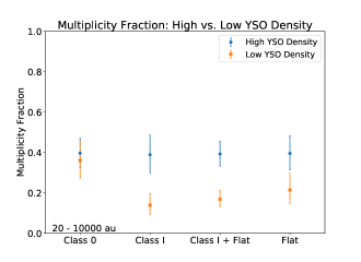
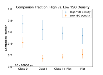
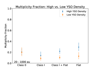
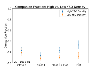
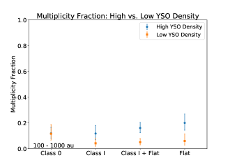
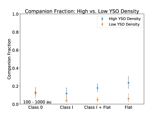
Figure 17: MFs and CFs on different scales as a function of protostar class for protostars residing at high ($\geq$30 pc^-2) and low ($<$30 pc^-2) YSO surface density. Regions with high YSO density have systematically larger CFs, and the MFs are also larger for Class I and Flat Spectrum protostars. For 20 to 10⁴ au separations, the MF differences between high and low YSO density are all $<$2$\sigma$, while the CF differences are $>$3$\sigma$ for Class I and Class I + Flat Spectrum and $\sim$1.8$\sigma$ for Class 0 and Flat Spectrum protostars. Class 0 protostars have comparable MFs and CFs for 20 to 10³ au and 100 to 10³ au, indicating primordial similarity of the multiplicity statistics in the Class 0 phase. The MFs and CFs are rising in the 20 to 10³ au and 100 to 10³ au ranges for the more-evolved protostars, which is interpreted as a sign of companion migration, see Section 4.5 and 5.3. However, the significance of the MF and CF differences are all $<$2$\sigma$ (see Sections 4.5 and 5.3).

We examined our Orion sample for differences in the multiplicity statistics between regions of high and low YSO density. YSO density is determined using YSO catalogs that are constructed from infrared samples (Megeath et al., 2012; Pokhrel et al., 2020) and completeness corrected using X-ray catalogs where available (Megeath et al., 2016). We set our boundary between low and high density regions at a YSO density of 30 pc^-2 such that there were comparable numbers of protostars in the regions assigned as high and low YSO densities. These MFs and CFs are listed in Table 7 Multiplicity and Companion Fractions at High and Low YSO Surface Densities, and we show them graphically for different ranges of separations in Figure 17. There are apparent differences in the MFs and CFs in the 20 to 10⁴ au separation range. The differences in the CFs between high and low YSO density regions are 1.8$\sigma$ for Class 0, 3$\sigma$ for Class I, 4$\sigma$ for Class I with Flat Spectrum, and 1.9$\sigma$ for Flat Spectrum on its own, while the differences in the MFs are not statistically significant. The difference in the CFs is also $>$3$\sigma$ when considering all classes together.

We now shift our focus to the smaller separation range between 100 to 10³ au in order to compare with Kounkel et al. (2016), although we also examine 20 to 10³ au because our data allow for smaller minimum separations. We find a tentative difference between the CFs for high and low YSO density regions for both the full sample and the combined Class I and Flat Spectrum sample. The Class I + Flat Spectrum sample has a 1.9$\sigma$ difference in the CFs between high and low YSO densities, while the difference in the CF for the Flat Spectrum sample alone is 1.5$\sigma$. The MF differences are less significant (at most 1.6$\sigma$) because the MFs are smaller than the CFs in this range of separations. If separations from 20 to 10³ au are instead considered, the differences are 1.4$\sigma$ and 1.8$\sigma$ for the Class I + Flat Spectrum and Flat Spectrum samples, respectively.

Finally, we note that only the Class 0 protostars do not exhibit significant differences in their MFs and CFs in separation ranges of 100 to 10³ au, 20 to 500 au, or 20 to 10³ au. Thus, the Class I and Flat Spectrum protostars are the only ones whose multiplicity properties may be to be sensitive to YSO density for the 100 to 10³ au separation range.

5 Discussion

The combined results for Orion and Perseus demonstrate the relative consistency for the same protostar classes. There are some differences in the separation distributions and MFs/CFs between protostar classes and with respect to high and low YSO densities. Furthermore, while not analyzed as part of this work, the MFs and CFs observed in Ophiuchus are found to be comparable to Orion and Perseus (Encalada et al., 2021). Characterization of the evolutionary classes in the Ophiuchus sample remains challenging, however (McClure et al., 2010), and there are substantially fewer Class 0 protostars compared to Orion and Perseus. Nevertheless, the consistency of multiplicity properties measured in different regions hints at common physical processes at work to give rise to the observed multiplicity, and the statistics afforded by these surveys enable further constraints on the evolution of multiplicity within the protostellar phase and the role multiplicity might play in protostellar evolution.

5.1 Formation Mechanisms of Multiple Systems

We detect multiple protostar systems with separations from 10s to 1000s of au (Figures 9 - 12), encompassing the range of physical scales where the disk ($\sim$10s to 100s of au) and infalling envelope (1000s of au) are the dominant physical structures. The most favored mechanisms for multiple star formation are disk fragmentation from gravitational instability (GI), operating on $\lesssim$500 au scales, and turbulent fragmentation operating on 100s of au scales and larger. Although turbulent fragmentation occurs on relatively larger scales, companions formed from this process can migrate from $\gtrsim$10³ au to less than 100 au in a few 100 kyr (Offner et al., 2010; Lee et al., 2019), and there is also evidence for smaller scale turbulent fragmentation in some numerical simulations (Bate, 2012). Thus, it is possible that both mechanisms produce companions with separations $\lesssim$500 au, while a single mechanism populates $\gtrsim$500 au. Dynamical interactions within higher order multiples can also contribute to substantial evolution of system separations (Kroupa, 1995; Bate et al., 2002; Sadavoy & Stahler, 2017; Cournoyer-Cloutier et al., 2021), either via the ejection of one component, or longer timescale secular mechanisms such as Kozai-Lidov oscillations (Fabrycky & Tremaine, 2007; Reipurth & Mikkola, 2012), though this is likely a smaller contribution (Moe & Kratter, 2018).

For the turbulent fragmentation and disk fragmentation mechanisms to operate, certain physical conditions are required. The main ingredients for turbulent fragmentation is dense gas and a turbulent velocity spectrum. The turbulence will create local regions of higher density, which can collapse to form stars if a region becomes becomes gravitationally bound and collapses. Simulations can produce this type of fragmentation in a variety of conditions with driven or decaying turbulence and in the presence or absence of magnetic fields (Offner et al., 2010; Bate, 2012; Li et al., 2018; Lee et al., 2019).

The fragmentation of disks to form companion stars broadly requires the presence of massive disks during the star formation process. The typical criterion used to describe disk stability is the Toomre Q parameter

$$Q=\frac{c_{s}\Omega}{\pi G\Sigma}.$$ (6)

Where $c_{s}$ is the sound speed of the gas, $\Omega$ is the angular velocity set by Keplerian rotation, $G$ is the gravitation constant, and $\Sigma$ is the gas surface density of the disk. Values of $Q$ near or below 1 have strong enough self-gravity relative to the sound speed and rotational shear that can lead to the formation of fragments in the disk as well as spiral arm formation (e.g., Kratter & Lodato, 2016). Also, Q is a function of radius, so portions of the disk can be unstable while other portions remain stable. Fragmentation will thus generally be most feasible in the outer disk where rotation is slower and the gas is cooler, so long as the surface density is not too low.

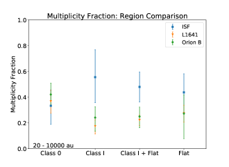
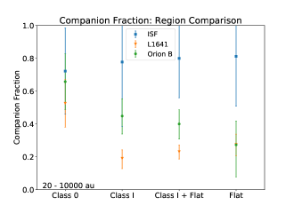
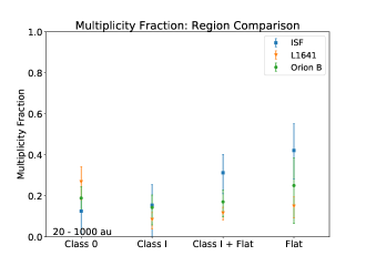
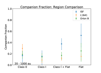
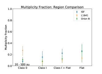
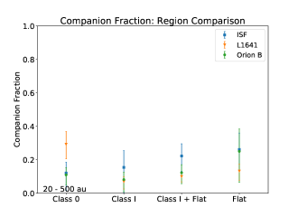
Figure 20: MFs and CFs on different scales as a function of protostar class for different regions within Orion. The MFs and CFs of the non-Class 0 protostars in the ISF are systematically higher than the other regions for separations 20 to 10⁴ au, but the differences are not statistically significant.

While turbulent fragmentation can produce multiples that are ultimately found on both large and small spatial scales, it is unclear whether this mechanism can create enough multiples that migrate to $<$500 au separations to reproduce the observations. Recent simulations by Lee et al. (2019) examined the formation of multiple systems from turbulent fragmentation and their subsequent evolution. The simulations did not have the resolution to resolve fragmentation within disks, but could track sink particle migration down to 10s of au scales. Thus, these simulations provide an estimate for the fraction of companions at $\lesssim$500 au separations formed via turbulent fragmentation with migration. Our observations for the combined Orion and Perseus samples find that the observed fraction of companions are $\sim$2-3 times larger on $\lesssim$500 au scales (depending on whether the full sample or only Class 0s are compared) than the fractions found in the simulations by Lee et al. (2019), see their Figure 20 vs. our Figure 12. Furthermore, studies by Cournoyer-Cloutier et al. (2021) with different models indicate that companions formed through dynamical capture in a forming cluster typically have separations $>$10³ au. This provides some evidence that at least half of the companions found on scales $\lesssim$500 au are likely to have formed via disk fragmentation. This agrees with $\sim$66% of close multiples in Perseus that were consistent with having formed via disk fragmentation based on their observed disk/envelope rotation on $<$500 au scales (Tobin et al., 2018).

While this comparison seems to suggest that disk fragmentation is important to forming multiples at $<$500 au, a simple characterization of gravitational instability for the disks in Orion in Paper I did not indicate a large number of Class 0 or Class I disks near the instability limit. Also, the average disk radius for Class 0 and I protostars in Orion is $\sim$40 au, rather than $\sim$100 au. This could pose a challenge to populate the $<$500 au multiples from disk fragmentation, unless gas masses were underestimated (which is certainly possible). Also, fragmentation can happen very quickly, on an orbital timescale ($\sim$10³ yr for $M_{*}$=1.0 M_☉ at 100 au). Therefore, the close multiples we observe could be the result of the disks that already fragmented, and the disks may not remain in a near-unstable state for long enough time to enable many of them to be discovered. For example, we did not detect obvious analogs to the fragmenting triple system L1448 IRS3B in Perseus (Tobin et al., 2016b; Reynolds et al., 2021) within Orion, and spatial resolution was too low to detect analogues to [BHB2007] 11 (Alves et al., 2019). We do note however that the instability calculations presented in Paper I made many simplifying assumptions to arrive at a disk-averaged limit, so those values should not be considered absolute.

As we discussed previously, contamination by chance alignments at large separations can artificially inflate the number of wide companions. This effect increases the apparent importance of turbulent fragmentation. Despite our attempts to mitigate the contribution of likely false associations (see light gray bars vs. dark gray bars in Figure 12), some contamination may still be present at large separations. The simulations from Lee et al. (2019) also characterize the number of true multiples versus the number of line of sight associations. They found that on scales $\geq$10³ au at least 50% of companions could be line of sight associations. Lee et al. (2019) note, however, that this result is partially due to a filamentary cloud that is oriented along one of the Cartesian axes, resulting in a large number of false associations, so 50% could be a worst case scenario. Furthermore, the numerical simulations did not have accompanying synthetic observations, but rather analyzed sink particle positions. Our observations here use the dusty circumstellar disks as signposts of multiplicity, which will not detect companions with 100% efficiency, as demonstrated in Section 3.6. Therefore, we expect that the simulations (when observational bias is not applied) will include more companions than observations detect. Consistent with this expectation, the histogram of separations from the Perseus protostars appears to agree well qualitatively with the Lee et al. distribution of true companions (see their Figure 20 on scales from $\sim$300 au to $\sim$3000 au.) Our estimates of contamination do not exceed $\sim$30% until separations $\gtrsim$3000 au (see Figures 9-12), and that contamination is not significant on scales $<$3000 au. This result is largely consistent with turbulent fragmentation simulations at these separations. Also, the use of dust continuum and free-free continuum as a probe of multiplicity implicitly creates a selection bias that may reduce our susceptibility to contamination by effectively requiring that protostars have a certain amount of circumstellar dust (or jet emission) to be detectable.

In summary, existing simulations of multiplicity originating from turbulent fragmentation alone do not produce sufficient numbers of companions at separations $<$ 500 au to explain the observations. Thus, we suggest that disk fragmentation is responsible for $\sim$50% of multiple systems with separations $<$ 500 au. Beyond 500 au separations, simulations of turbulent fragmentation are able to reproduce the observations. Therefore, we expect that the observed separation distributions result from both disk fragmentation and turbulent fragmentation, and disk fragmentation is expected to be most likely in the Class 0 phase when the disks have the most mass (Tobin et al., 2020).

5.2 Future Evolution of the Companions

The view of multiplicity obtained toward the protostars in our sample is a single snapshot in the evolution of these systems, and the separations of the observed systems will continue to evolve during protostellar evolution and beyond. Here we discuss the evolution that we expect to occur in the context of our observational knowledge of multiplicity in later stages of the star formation process and field stars.

5.2.1 Evolution within the Protostellar Phase

While our observed multiplicity properties may not have significant contamination from unrelated protostars at scales $<$3000 au, our observed distribution of separations for all protostar classes does not imply that all of these associated protostars are going to remain bound systems and/or at their current separations. The functional form of the separation distribution of field solar-type stars from Raghavan et al. (2010) is overlaid on the separation distributions in Figures 9 - 12 (also see Figure 14). The histograms of separations are quite inconsistent with the field solar-type stars on scales $\gtrsim$10³ au, and we can rule out that they are drawn from the same parent distribution for most protostar classes, except the most evolved sub-samples, see Section 4.3.4.

Thus, either a large number of the current protostellar companions between 10³ to 10⁴ au must migrate to smaller separations or they must become unbound. It is also important to point out that most protostars observed in this study will become M-stars rather than solar-type stars, and main-sequence M-stars (M$\sim$0.3 M_☉) have a separation distribution that is even more skewed to smaller separations. Solar-type stars have a mean separation of 50 au (Raghavan et al., 2010), while M-stars have a mean separation of $\sim$20 au (Winters et al., 2019). Therefore, it is likely that most of the systems that we study here–and remain multiples into the main sequence–will ultimately have a mean separation of $\sim$20 au.

It is noteworthy that the study by Lee et al. (2019) found a similar fraction of companions from $\sim$500 to 3000 au as our observations in Perseus, in addition to Orion. However, the companions studied in Lee et al. (2019) were indeed bound when only considering the sink particle mass and did not need to consider the surrounding gas mass potential. Thus, companions must either continue to evolve to smaller separations, become unbound through $\geq$3-body interactions, or have formed with unbound relative velocities. Lee et al. (2019) noted that only when the gas mass is comparable to or exceeding the sink mass was the boundedness affected by the surrounding gas potential. Class 0 protostars tend to have a larger number of companions separated by greater than 10³ au (Figures 12 and 16), and these systems are the most likely to have an envelope mass greater than the stellar mass. We therefore argue that in order for the separation distributions of Class 0 protostars to evolve toward the field solar-type distribution (Class I and Flat Spectrum as well), under the assumption that most companions from 500 to 3000 au are bound, two processes must be at work. First, protostellar multiples with current separations greater than 10³ au may have companions that are lost due to either being unbound or becoming dynamically unbound due to loss of gas mass by outflow expulsion or interactions (e.g., Offner & Arce, 2014; Sadavoy & Stahler, 2017). Second, many of those that do not become unbound must migrate to smaller separations. Some may migrate from $>$ 10³ au to $\sim$100s of au, while those that may have formed at $\sim$100 au can migrate to $<$ 30 au. The migration to $<$ 30 au is necessary to dilute the peak in separations at $\sim$100 au observed for Class 0 protostars and produce the larger number of multiples found toward main sequence stars at separations $<$ 50 au. The statistical significance in the difference of the separation distributions for Class 0 protostars with respect to the more evolved Flat Spectrum is further evidence that separations evolve with protostellar evolution (Figures 9 and 10 (Section 4.3.2). This will be discussed further in the following sections.

At present, it is unclear how quickly protostellar separations can evolve to $<$ 30 au given that our spatial resolution is limited to $\sim$20 au in Perseus and Orion. Companions with sub-au separation likely exist by the Class I phase from radial velocity observations of embedded sources (Viana Almeida et al., 2012) and of some exotic phenomena like pulsed accretion (Muzerolle et al., 2013), but statistics are clearly lacking. ALMA can probe scales $<$ 10 au at the distances to nearby star-forming regions, but such observations are only available for a handful of protostars.

Even with better spatial resolution, there are a number of complicating issues that may cause incompleteness in multiplicity characterization at $<$ 30 au scales when using observations of dust continuum. As companions with smaller separations are examined, the amount of dust mass that can reside in circumstellar disks decreases, rendering them less detectable due to disk truncation (Artymowicz & Lubow, 1994). Also, even if a small circumstellar disk has a high surface density, dust opacity will limit the emergent flux density, depending on wavelength. This could cause some circumstellar disks to blend with their circumbinary disks which could be the case of HOPS-361-C and HOPS-288 (Figure 3). Thus, centimeter wavelengths remain important given than they can pierce through highly obscuring dust, and free-free emission at these wavelengths can provide another signpost of multiplicity that will be useful toward smaller separations.

5.2.2 Evolution Beyond the Protostellar Phase

The results from this study as a whole, and the Class 0 protostars in particular, establish the starting point for multiplicity evolution as a bimodal distribution of separations. This distribution of separations for Class 0 protostars is inconsistent with solar-type field stars and more evolved Flat Spectrum protostars. However, it is not possible to rule out that Flat spectrum protostars are drawn from the same parent distribution as field stars, affirming that the log-normal fit to the Raghavan et al. (2010) sample appears similar to the most-evolved protostar samples. Furthermore, the MFs and CFs for the most evolved protostars on all scales are consistent with those of the field stars, while the CF of Class 0s is inconsistent by $>$ 3$\sigma$ (Figure 16).

Observational evidence from our survey alone therefore indicates that an initially bimodal distribution of separations can evolve toward the observed field distribution. Moreover, models that include prescriptions for turbulent fragmentation, disk fragmentation, gas-driven migration, and dynamical upheaval can reproduce the observed separation distribution of field multiples, when assuming an initially bimodal distribution of protostellar companions (Moe & Kratter, 2018; Tokovinin & Moe, 2020). Given that the most evolved protostars cannot be statistically distinguished from the field separation distribution, the question arises as to whether most of the multiplicity evolution occurs during the protostellar phase. If true, this implies that the presence of circum-multiple material is the primary driver of multiplicity evolution and once the gas is accreted or expelled, rapid reorganization is no longer possible and must occur via n-body interactions.

Thus, more evolved Class II and III YSOs represent the obvious population to study in order to answer the aforementioned question. For separations $<$10 au, Class II and Class III YSOs are consistent with the field star multiplicity (Kounkel et al., 2019). Such close systems cannot typically be detected toward protostars, aside from a few special cases (e.g., Ortiz-León et al., 2017; Maureira et al., 2020). For separations between $\sim$100 au to 1000 au, the MFs/CFs and separation distributions of most YSO populations agree well with the field (aside from Taurus-Auriga) (Reipurth et al., 2007; Kraus et al., 2011; King et al., 2012; Duchêne et al., 2018), and the MFs/CFs of protostars in our sample are also in good agreement for this range.

On the other hand, the MF and CF in the separation range of $\sim$10-60 au for YSOs in Orion can exceed those of the field by a factor of $\sim$2 (CF = 0.218${}^{+0.08}_{-0.051}$), with 1.7 to 2.7$\sigma$ significance relative to field solar-type stars and M-type stars, respectively (Duchêne et al., 2018). We note, however, that De Furio et al. (2019) did not confirm this result for M-stars in Orion. The separation distributions of YSOs in different star-forming regions sampled from 19 to 100 au may also not be statistically consistent with each other or the field (King et al., 2012). This range of separations is unique because systems with such separations will not be dynamically altered once the disk(s) has dissipated in all but the highest density cluster environments. Tables The VLA/ALMA Nascent Disk and Multiplicity (VANDAM) Survey of Orion Protostars V. A Characterization of Protostellar Multiplicity and The VLA/ALMA Nascent Disk and Multiplicity (VANDAM) Survey of Orion Protostars V. A Characterization of Protostellar Multiplicity show that there are only 13 multiples (10 Orion, 3 Perseus) with separations between 10 and 60 au (MF/CF=0.027 $\pm$ 0.01) and 34 (25 Orion, 9 Perseus) companions from 10 to 100 au (MF/CF=0.07 $\pm$ 0.01). Thus, from 10 to 60 au our observations are statistically inconsistent with those of Duchêne et al. (2018) at $>$3$\sigma$ significance, then compared to King et al. (2012) we are at most 2$\sigma$ different from the regions with the highest CFs. We did not compare separation distributions given the small number of separations for the protostar samples.

Taken at face value, the discrepancy between our survey and that of Duchêne et al. (2018) is quite large and could imply that more companions must migrate inward to 10 to 60 au separations following the Flat Spectrum phase. However, there are no extremely large excesses of companions in the separation distributions (Figures 9-11 for Class I and Flat spectrum protostars except beyond 3000 au and the migration timescales will likely not align with the evolution timescale from Flat Spectrum to Class II.

We instead argue that incompleteness in our survey between 10 and 60 au enhances the disagreement. Our raw angular resolution limit is $\sim$20-30 au and to reach the highest resolutions the noise is increased and the emission from companions must be bright enough to be detected. Thus, millimeter/centimeter measurements of multiplicity also likely suffer from a bias analogous to the Branch bias (Branch, 1976) known in visible-light studies where stellar twins are easier to detect and more complete than systems with fainter companions. But, unlike visible light studies, we cannot easily correct our data for this bias, because there is no expected distribution of companion flux densities. Also, at our observed resolution, many sources are marginally-resolved (Paper I) due to the dust emission probing their circumstellar disks), which will further reduce sensitivity to close companions. This is in addition to other mitigating factors discussed in Sections 3 and 5.1 which could limit our ability to detect companions at millimeter/centimeter wavelengths due to dust opacity and contrast of circumstellar emission to optically thick circumbinary emission. Further investigation is therefore required to determine if there is truly an inconsistency between our protostellar sample and more-evolved YSOs in the separation range 10 to 100 au.

5.3 Multiplicity Variation with YSO Density: A Sign of Migration?

The observed differences in the separation distributions, MFs, and CFs as a function of protostellar class, suggest that the number of (detectable) multiples and shape of the separation distributions evolve over time (Figures 9 - 12, 15, and 16). This implies that there may be more direct evidence for how and when companion migration occurs in our sample statistics. We specifically focus on the 100 to 10³ au separation range. This is the range of separations that must be traversed if companions formed at $>$10³ au separations migrate inward to further populate separations $<$100 au.

We then further examine the MFs and CFs as function of protostellar class separately for regions of high and low YSO density (Figure 17). Within the 100 to 10³ au separation range, there are higher MFs and CFs in Orion for the combined Class I + Flat Spectrum sample and the Flat Spectrum sample alone in regions of high YSO density versus low YSO density; however, we note that the significance the CF differences are only 1.9$\sigma$ and 1.5$\sigma$, respectively, and the MF differences are at most 1.6$\sigma$. Then Class 0s exhibit comparable MFs and CFs at both high and low YSO densities for the same separation range. This finding for Class I and Flat Spectrum protostars is consistent with a previous near-infrared study in Orion by Kounkel et al. (2016). The difference between Class I and Flat Spectrum MFs and CFs in regions of high vs. low YSO density, while the Class 0s statistics remain similar, may be a sign of migration.

The fact that the MFs or CFs for the Class 0 samples at high and low YSO densities are consistent in the separation ranges from 20 to 500 au, 20 to 10³ au, and 100 to 10³ au implies that the observed companions in these ranges are mostly primordial (Figure 17), meaning that they most likely formed near where we currently observe them. However, on 20 to 10⁴ au scales, the CF of Class 0 protostars is $>$2$\times$ higher at high YSO densities than at low YSO densities, with a 1.8$\sigma$ difference. This leads us to suggest that Class 0 protostars have a reservoir of young, higher-order companions that could migrate to smaller separations through the 100 to 10³ au separation range at later times, particularly in the regions of high YSO density.

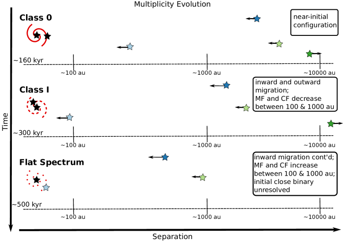
Figure 18: Illustration of our proposed scenario for migration to explain the MF and CF changes from Class 0 to Flat Spectrum on 100 to 1000 au separations as shown in Figure 17 for YSOs in regions with high YSO density. We begin with a Class 0 system at the top that forms an initial binary within its disk (black stars and red spiral), but in its vicinity another protostar formed between 100 and 1000 au and three more between 1000 and 10000 au. As an example, the three nearest protostars at $>$100 au have net inward velocities, while the outermost star (red) has an outward net velocity. By the Class I phase, after $\sim$160 kyr, the inner binary (black stars) has become closer and the protostar that was originally between 100 and 1000 au is now at $<$100 au. Then, two of the widely separated protostars have begun to migrate inward, but are still at $>$10³ au, and one protostar (red) has moved to $>$10⁴ au and is no longer considered a companion. This scenario could explain the slight drop in MF and CF between 100 and 10³ au for Class Is. Finally, by the Flat Spectrum phase, after $\sim$300 kyr, the initial inner binary shrunk to $<$30 au and is no longer resolved, but a companion that was previously between 100 and 10³ au is now orbiting the close binary. Then the two protostars that were initially $>$10³ au (but were migrating inward) are now located between 100 and 10³ au. Thus, this could explain the rise in MF and CF for Flat Spectrum protostars that are expected to be among the most evolved in our sample.

We suggest that the overall larger number of wide companions in high YSO density regions for Class 0 protostars results in larger MFs/CFs in the 100 to 10³ au separation range for Class I and Flat Spectrum protostars at high vs. low YSO density. This is only true for more evolved protostars because of the time lag between formation and migration to smaller separations. We provide a sketch of our proposed scenario in Figure 18. Thus, if our interpretation is correct, we can constrain the typical migration timescale to be longer than the Class 0 lifetime, but shorter than the lifetime of Class I and Flat Spectrum protostars. The Class 0 phase is only expected to last $\sim$160 kyr (Dunham et al., 2014), but it could be shorter (Kristensen & Dunham, 2018). Class I and Flat Spectrum protostars, on the other hand, are expected to be at least $\sim$100 to 300 kyr older than Class 0 protostars (Kristensen & Dunham, 2018; Dunham et al., 2014), allowing a longer timescale for migration to take place. Therefore, a typical timescale for migration from $>$10³ au to $<$10³ au is between $\sim$0.2 and 0.5 Myr. This proposed timescale based on the evolutionary classes is consistent with the migration timescale from $>$10³ au separation to $\lesssim$100 au predicted in numerical simulations by Offner et al. (2010), when magnetic fields were not included, and Lee et al. (2019) with magnetic fields. Both indicate that there would be too little time for significant migration from $>$10³ au during the Class 0 phase.

Finally, prior observations suggest that companions are also migrating to separations smaller than 20 au (separations below our resolution limit) during this timeframe (see Figure 18, and Muzerolle et al., 2013; Moe & Kratter, 2018; Kounkel et al., 2019). However, our results indicate that companions with separations between 100 to 10³ au are replenished via migration faster than they are depleted by migration to separations $<$ 20 au. We do not expect significant formation of companions in situ for Class I and Flat Spectrum protostars because their envelopes are significantly reduced in mass and density (Furlan et al., 2016), and their disks are systematically lower in mass, making disk fragmentation at the Class I and Flat Spectrum stage unlikely (Paper I). Thus, inward migration from initial separations $>$10³ au is a likely explanation for the increased MFs/CFs from 100 to 10³ au for Class I and Flat Spectrum protostars. This inward migration from $>$10³ au is primarily caused by dynamical friction with the gas surrounding the protostars (Lee et al., 2019). It is possible that close dynamical interactions may produce ejections from small separations to larger separations, but the small number of triples with separations $<$ 500 au makes this mechanism unlikely. Capture during dispersal of small clusters is also possible (Moeckel & Clarke, 2011; Cournoyer-Cloutier et al., 2021), but this mechanism is relatively inefficient, not likely to produce the increases in MF and CF observed in the Class I and Flat Spectrum protostars, and does not produce the separation distributions we observe. Finally, our previous analysis suggests the likelihood of contamination by non-physically associated sources in the 100 to 10³ au separation range is low, providing further evidence in favor of this interpretation.

Consequently, the increase in the MF and CF between 100 and 10³ au for the Class I+Flat Spectrum sample (and the full sample) for protostars found in regions of high YSO density versus low YSO density points to the fragmentation properties of the molecular cloud indirectly playing a role in setting the MF and CF on this spatial scale in particular. This is because regions of higher YSO density have a strong correlation with higher gas surface density (Gutermuth et al., 2011; Pokhrel et al., 2020). Then, turbulent fragmentation of this dense gas likely plays a role in creating YSOs that have initially wide separations ($\gtrsim$10³ au). This means that in regions of high YSO density, there will be more companions with wide separations with respect to regions with low YSO density. The regions with lower YSO density can be assumed to have had less dense gas, making those regions less susceptible to the formation of companions with initial separations $\gtrsim$10³ au (e.g., Padoan & Nordlund, 2002; Bate, 2012; Offner et al., 2016; Krumholz et al., 2016). Thus, there will then be a smaller population of $>$10³ au companions initially that would be able to migrate to smaller orbits in regions of low YSO density.

To summarize, Class 0 protostars in regions of high and low YSO density have similar multiplicity fractions, indicating that companions on scales less than 10³ au tend to form with the same frequency. There is little time for migration during the Class 0 phase, so the MFs and CFs are comparable in regions of high and low YSO density for separations $<$10³ au. However, the Class 0 CF from 20 to 10⁴ au at high YSO densities is $>$2$\times$ (and 1.8$\sigma$) larger than at low YSO densities (Figure 17). Then, the larger MFs and CFs for Class I and Flat Spectrum protostars for regions of high versus low YSO density (and the lack of variation for Class 0 MFs/CFs) suggest that the differences may arise during evolution (Figure 18). Furthermore, regions of high YSO density are more likely to form more higher-order systems with $>$10³ au initial separations than low YSO density regions, and the time it takes for these protostars to migrate to the 100 to 10³ au separation range is comparable to the expected age of protostars in the Class I and Flat Spectrum sample. Thus, the increase in MFs and CFs of Class I + Flat Spectrum protostars and Flat Spectrum Protostars alone at high vs. low YSO densities could be evidence that migration is occurring and populating the range of intermediate separations. We caution, however, that the CFs of these samples for high and low YSO density regions only differ by 1.9$\sigma$ and 1.5$\sigma$, while the MFs differ by $\sim$1$\sigma$ to 1.6$\sigma$. Thus, while the proposed scenario is plausible, better statistics are required to reach higher statistical confidence. Better statistics would likely require combining multiple star-forming regions, since the sample of Orion protostars is highly complete.

5.4 Multiplicity of Class I and Flat Spectrum Protostars and Impact on Class Lifetime

Throughout this paper we have discussed the multiplicity statistics of the different protostellar evolutionary classes, but we have not discussed whether multiplicity affects protostellar evolution between classes. We highlighted in Section 4.4 that Flat Spectrum protostars are more often found in binary or multiple systems than Class I protostars. The MFs and CFs of Orion Flat Spectrum protostars are all larger than those of Class Is at all ranges of separations. However, we do note that the differences are generally only 1-1.5$\sigma$, so the trend is not statistically robust. The more evolved Flat Spectrum protostars are not significantly different from the Class I protostars in terms of luminosity or 0.87 mm flux density (though they are slightly fainter systematically; Paper I). The classification of Perseus protostars does not distinguish between Class I and Flat Spectrum protostars (Enoch et al., 2009), so it is unclear whether the difference exists there as well, but the numbers are smaller in Perseus, so differences will be more uncertain.

Given the estimated total lifetime of the protostellar phase ($\sim$1 Myr; all class lifetimes combined), we do not expect that star formation conditions change significantly over this short timespan in a way that could affect the number of multiples formed for Class Is (younger) relative to Flat Spectrum (older). Therefore, we instead suggest that multiple star formation within a core itself and/or the likely migration of companions (Figure 18) could speed up the transition between classes, resulting in a later evolutionary class having more multiples than the earlier classes. This could happen in a few ways, some of which would happen separately and some could be happening simultaneously, compounding the effect. First, outflows from two protostars within a dense core will be able to entrain and expel the dense gas faster. Second, consider a protostar formed via turbulent fragmentation that migrates closer to a companion. If the two protostars have misaligned outflows (e.g., Yıldız et al., 2012; Offner et al., 2016; Lee et al., 2016; Tobin et al., 2018), the outflows can more efficiently clear envelope gas as their separation contracts. Furthermore, the interaction of companions migrating in this way may cause the outflows to change direction over time leading to even more rapid clearing of envelope material than two misaligned outflows whose directions are not changing. Third, protostars separated by a few $\times$ 100 au (whether formed there or migrated to that location) will accrete from a larger volume of the envelope, reducing the central envelope density more quickly than a single protostar. These protostars can also have misaligned outflows, even if they both formed near those locations originally. Indeed, the systematically higher luminosities for multiples (Figure 8) is evidence that accretion may be more rapid in multiple systems.

All these scenarios will impact the evolution of the gas distribution in the inner envelope, thereby reducing the material responsible for emission between $\sim$10 to $\sim$160 µm (from reprocessed shorter wavelength radiation from the protostar and accretion). SED modeling of all the HOPS protostars found that Flat Spectrum protostars have lower envelope densities than Class Is. Thus, the SED slope from the near-infrared to the mid-infrared of multiple protostar systems could be intrinsically more shallow. This may be true whether the components of the multiple systems are coeval or not (Murillo et al., 2016). We conclude by suggesting that multiplicity and the reorganization of multiple systems that likely follow the Class 0 phase causes the protostar system to more rapidly evolve through the Class I phase to become a Flat Spectrum protostar.

In addition to the impact the multiples have on the envelope, they will impact the disks as well. Harris et al. (2012) found that disks toward Taurus multiples are detected less frequently than toward single stars. Then, Akeson et al. (2019) find that binary Class II systems follow a similar dust disk mass to stellar mass relationship as single Class II systems, but this relationship is shifted to lower disk masses. Furthermore, the disk radii in close binaries are also found to be tidally truncated (Manara et al., 2019), consistent with theoretical predictions (e.g., Artymowicz & Lubow, 1994). These findings indicate that the presence of a companion will likely increase the rate of disk dispersal. Such a mechanism may explain the lack of detection by ALMA toward a small number of Class I and Flat Spectrum multiples that are detected by HST (see Section 3.6).

5.5 Coevality of Multiples

In this section, we examine the co-evality of multiple systems in Orion by considering systems composed of different protostellar classes. It is important to stress, however, that while class is used as a proxy for age, the absolute ages of protostar systems are unknown. Murillo et al. (2016) examined the coevality of multiples in Perseus, finding that 33% of multiple systems are likely non-coeval, as measured by the fraction of systems with mixed evolutionary classes. A limitation to this analysis, however, is that independent class identifications for individual members can only be made for multiples with separations $>$10³ au and companions $<$10³ au are assumed to be in the same class.

To estimate the number of systems with a non-coeval member, we count the relative number of multiple systems that contain members with different evolutionary classes and those that contain members of the same class (see Table 5 Orion and Perseus Multiplicity and Companion Fractions with Probabilities). Of the multiple systems identified, 42% of Class 0 multiple systems have a non-coeval member compared to 22% of Class I systems, and just 4% of Flat Spectrum systems have a non-coeval member. In total, the number of systems with a non-coveal member is 25%, which is comparable to results from Perseus.

One interesting point is that the majority of non-coeval systems are Class 0 systems. This implies that non-coeval systems are frequently associated with the most recent epoch of protostar formation, and hence, the presence of dense gas. However, the estimated lifetimes of the Class 0, I, and Flat Spectrum phases are $\sim$0.15, 0.35, 0.4 Myr (Dunham et al., 2014), so the estimated age difference between Class 0 and Flat Spectrum systems is not large. In Sections 5.1 and 5.2, we discussed in how turbulent fragmentation most likely forms widely separated systems, which migrate to different separations over time. Furthermore, the free-fall time of gas with a typical dense core density of $\sim$10^5-6 cm^-3 (Bergin & Tafalla, 2007) is $\sim$0.05-0.15 Myr. Thus, it is plausible for star formation to occur with asynchronicity over the size scale of a star-forming core due to turbulent fragmentation, which can lead to the appearance of non-coeval systems.

The apparent lack of non-coeval members within systems dominated by Flat Spectrum protostars can be understood in a couple ways. First, star formation in regions dominated by Flat Spectrum protostars may have largely finished. In addition, the Flat Spectrum lifetime is expected to be longer than the Class 0 lifetime, so the evolution of one member could catch up with the evolutionary state of other members. Another possibility is that Flat Spectrum protostars have more time to migrate away from their birth sites and are more likely to leave a particular system (e.g., Figure 18), potentially leaving systems with less Flat Spectrum members. Thus, the various outcomes of turbulent fragmentation can naturally explain both the formation of and the prevalence of apparent non-coeval systems in those dominated by Class 0 protostars, as well as the lack of non-coeval Flat Spectrum systems.

Overall, taking the class assignments of protostars at face-value, our data also seem to support the idea of non-coeval formation of companions. However, a combination of effects like gas configuration, envelope asymmetry, efficiency of gas removal by outflows, and relative inclinations/orientations can lead to systems appearing non-coeval, even when they are indeed coeval. Furthermore, accepting that some systems are indeed non-coeval, the absolute age differences that correspond of these systems are small compared to the expected lifetimes of the stars. So whether a multiple system was coeval or not (having the same evolutionary class at the observed time, by our definition) is not likely affect stellar evolution. Moreover, such small age differences, like the difference in expected ages between Class 0 and Flat Spectrum protostars ($\sim$0.35 Myr), will not impact later diagnostics of pre-main sequence age like Lithium abundances and differences in location on pre-main sequence evolutionary tracks will not be significant.

6 Conclusions

We have conducted a multiplicity analysis of protostars in the Orion A and B molecular clouds using data taken with ALMA (0.87 mm) and the VLA (9 mm) toward 328 protostars that have been classified with both Spitzer and Herschel. We have also reanalyzed previously obtained data from the Perseus molecular cloud (Tobin et al., 2016a) to enable a consistent comparison of these data and Orion. Our main results are as follows:

• We have characterized the multiplicity fractions (MFs) and companion fractions (CFs) for Orion, Perseus, and the two samples combined, we also sub-divide the MFs and CFs by separation and protostellar class. Using the full range of separations (20 to 10⁴ au) the MFs of Orion and Perseus are 0.30$\pm$0.03 and 0.38$\pm$0.07, respectively, and the CFs are 0.44$\pm$0.03 and 0.57$\pm$0.07, respectively. The combined MF and CF within the same separation range are 0.32$\pm$0.02 and 0.46$\pm$0.03, respectively.

• We find that MFs and CFs for 20 to 10⁴ au separations decrease from Class 0 to Class I, and Flat Spectrum protostars are consistent with Class I. However, at separations less than 10³ au Flat Spectrum protostars can have higher MFs and CFs relative to Class Is in Orion as a whole and in each sub-region of Orion, but the differences are only at the 1 to 1.5$\sigma$ level. If the difference is real this could be evidence that multiplicity speeds up evolution through Class I to Flat Spectrum.

• We characterize the separation distributions for Orion and Perseus, both as a whole and divided by protostellar class. The overall and Class 0 samples appear bimodal with peaks near $\sim$100 au and $\sim$3000 au. This bimodal appearance is driven by the Class 0 sample, since the Class I and Flat Spectrum samples do not appear bimodal on their own. Thus, Class 0 protostars have the most companions between 20 to 500 au separations and at $>$10³ au. A statistical comparison between the Orion and Perseus separation distributions does not reveal any statistically significant differences between the two regions.

• Statistical evidence shows that the separation distributions for Orion Class 0s and Orion Class Is [Class 0–(Class 0, Class I, Flat) and Class I–(Class 0, Class I, Flat)], are inconsistent with being drawn from a log-flat distribution of separations. Class 0 protostars [Class 0–Class 0 and Class 0–(Class 0, Class I, Flat)] are also statistically inconsistent with the separation distribution for field solar-type stars. This indicates that the bimodal separation distribution apparent in histograms may be robust and that significant evolution of these separation distributions is required to produce the field separation distributions for solar-type and M-type stars from the Class 0 separation distributions. The separation distributions for Flat Spectrum protostars, however, are statistically consistent with the separation distribution of field solar-type stars.

• We find that protostars with higher surrounding YSO densities have correspondingly higher MFs/CFs, in agreement with previous results from Kounkel et al. (2016). We find that the MF and CF for Class 0 protostars on 20 to 10⁴ au separations is higher relative to Class I and Flat Spectrum protostars at both high and low YSO densities. This is due the larger frequency of higher order multiples present in Class 0 protostars. However, the MF differences are only at the 1$\sigma$ level, while the CF differences are at the 1.5$\sigma$ to 1.9$\sigma$ level. Some of these companions at $>$10³ au are expected to migrate through the 100 to 10³ au range and contribute to the elevated MFs ($\sim$1$\sigma$ differences) and CFs (1.5$\sigma$ - 1.9$\sigma$ differences) observed toward Class I + Flat spectrum protostars and Flat Spectrum protostars alone on these scales in regions with high YSO densities. Also, the MFs and CFs for Class 0 protostars showed no differences between high and low YSO densities for the separation ranges of 20 to 500 au, 20 to 10³ au, and 100 to 10³ au. We therefore suggest that the Class 0 MFs and CFs within these ranges of separation are primordial and the MF/CF increase of Class I + Flat Spectrum and Flat Spectrum protostars for 100 to 10³ au separations could be due to migration.

• We find more companions with separations from 20 to 500 au than predicted by numerical simulations that form multiples only via turbulent fragmentation (e.g., Lee et al., 2019). This suggests that both disk fragmentation and turbulent fragmentation with migration are needed to produce the observed population of close multiple systems.

• The distribution of bolometric luminosities for single and multiple protostars are found to have statistically significant differences. The median luminosity of single protostars is found to be 0.96 L_☉, while the median luminosity of multiple protostars is 3.27 L_☉. The higher luminosities could result from both higher accretion rates in multiples and/or multiple protostars accreting at the same rate.

• We compare near-infrared and millimeter detection statistics for those multiple systems in Orion with overlapping observations with Hubble Space Telescope observations at 1.6 µm and ALMA and/or the VLA. Comparing the sample of protostars observed at both near-infrared and radio/sub-millimeter wavelengths and in the same 100 to 10³ au separation range. We find that the incompleteness of the millimeter-only studies is 20% for samples of Class 0, Class I, and Flat Spectrum protostars, and this rises to 29% if the sample is limited to Class I and Flat Spectrum protostars. The near-infrared is 31% incomplete for samples of Class 0, Class I, and Flat Spectrum protostars, but if only Class I and Flat Spectrum protostars are sampled, the incompleteness drops to 11%. This finding is in part due to the inability of HST to directly detect Class 0 protostars and many Class I protostars at 1.6 µmdue to their embedded nature.

• Dust opacity at millimeter/submillimeter wavelengths can play a role in the ability to detect companions with separations $<$200 au. We find that three systems only have VLA (9 mm) detections of their companions that were undetected by ALMA at 0.87 mm. The non-detection by ALMA is most likely due to the high optical depth of the surrounding dust emission, obscuring the companion at shorter wavelengths. There are further two tentative companions that are detected by the VLA but not by ALMA, likely for the same reason. Future studies must remain cognizant of this potential observational bias when observing at submillimeter and millimeter wavelengths.

The statistics on protostellar multiplicity from this survey have resulted in a robust characterization of the starting point for multiplicity evolution. The data indicate that similar processes produce the observed populations of protostellar multiples in Orion and Perseus; however, it remains to be seen if all nearby star-forming regions and isolated cores have consistent multiplicity properties. The most populous regions without comprehensive surveys are Serpens/Aquila and the California Molecular Cloud. In addition to obtaining greater statistics in the nearby regions at similar spatial scales, it is also important to probe closer separations in the protostellar phase in order to understand how close multiples form and evolve. ALMA, in addition to future instruments like the ngVLA, SKA, and 30 m class telescopes will be essential for characterizing multiplicity at the closer separations.

Appendix A Use of Companion Probabilities in Multiplicity Characterization

A.1 Probability of a Detected Source being a Companion

The multiple systems in our sample may be contaminated by chance alignments with other YSOs in the Orion cloud, with the probability of contamination increasing as separation increases and higher local YSO surface densities. We attempt to account for this effect in our algorithm as follows. We begin by estimating the typical YSO surface densities. We used the surface density of YSOs measured toward each protostar position, using the 11th nearest neighbor, and then dividing 10 by the area of a circle at the radius of the 11th nearest neighbor to determine the local YSO surface density ($\Sigma_{YSO}$; e.g., Gutermuth et al., 2005, 2011; Megeath et al., 2016). The protostar, whose surrounding $\Sigma_{YSO}$ is being measured, is not included in the count of the 11 nearest neighbors. This results in an uncertainty of 33% in the $\Sigma_{YSO}$ measurement (Casertano & Hut, 1985); equations describing the surface density estimator are provided in Megeath et al. (2016). The YSO surface densities for Orion and Perseus are provided with the input catalogs in Tables The VLA/ALMA Nascent Disk and Multiplicity (VANDAM) Survey of Orion Protostars V. A Characterization of Protostellar Multiplicity and 2 Perseus Catalog.

For the protostars in Orion, we used the catalog of probable YSOs from Megeath et al. (2012), and then for Perseus we used the YSO catalog of Perseus from the Spitzer Extended Solar Neighborhood Archive (SESNA) catalog (Pokhrel et al., 2020, Gutermuth et al. in prep.). If there was no source in the catalog within 2$\farcs$5 of an ALMA or VLA detection, the ALMA or VLA source was added to the catalog for computation of the YSO surface density. The YSO surface densities of Orion were corrected for completeness using X-ray catalogs when available (Megeath et al., 2016); the Perseus catalog did not undergo such a correction. For cases where a YSO was more isolated or did not have enough data of its surrounding region, we adopted the nearest measured YSO surface density value in our sample.

The YSO surface density toward each protostar provides an expectation value for the number of YSOs present within a given area around the protostar. Since nearly all the protostars in Perseus and Orion are contained within our samples, contamination is expected to come from disk-bearing YSOs. Based on our survey dust mass sensitivity of $\sim$1 M_⊕, compared to deeper surveys of YSOs in Lupus (Ansdell et al., 2016), we would detect 75% of disk-bearing YSOs. The detection probability follows a Poisson distribution

$$P(k)=\frac{\lambda^{k}e^{-\lambda}}{k!}$$ (A1)

where $\lambda$ = 0.75$\Sigma_{YSO}$ $\pi d^{2}$ and $k$ is the number of YSOs expected. $\Sigma_{YSO}$ is the number of YSOs per square parsec, and $d$ refers to the projected sky radius considered for calculating the probability of a random YSO. Thus, the probability of detecting $\geq$ 1 unassociated YSOs is 1 - P(0), where

$$P(\geq 1~{}YSO)=1.0-e^{-0.75\Sigma\pi d^{2}}.$$ (A2)

We ultimately need to determine the probability of whether a detected source is a companion or not. For this we make use of Bayes Theorem to determine

$$P(companion|detection)=\frac{P(detection|companion)P(companion)}{P(detection)}.$$ (A3)

Simply stated, given a detection, Equation A3 yields the probability of that detection being a companion. $P(detection|companion)$ refers to the probability that we would indeed detect a companion when there is one present. We assume that $P(detection|companion)$ = 0.75, because, as mentioned above, our sensitivity is expected to detect 75% of YSOs, which also applies to protostars, under the assumption that they are drawn from the same general population of dusty disks. We find that if we used values anywhere between 0.25 to 0.9, the probability of a given continuum detection being a companion is not significantly changed; in any event 0.75 is likely a reasonable estimate.

$P(detection)$ is the likelihood that we detect a source regardless of it being a companion or an unassociated source. Thus, we have

$$P(detection)=0.75~{}P(companion)+(1-e^{-0.75\Sigma\pi d^{2}})(1-0.75~{}P(companion)).$$ (A4)

The first part of the equation, $0.75~{}P(companion)$, is the probability of detecting a companion, while the latter part of the equation is the probability of finding a detection if there is no companion (i.e., an unassociated source). The factor of $(1-0.75~{}P(companion))$ is important, because this will balance the probability of detection in the event that $\Sigma$ is very large. If we did not include the 0.75 factor, $P(detection)$ would always be less than 1 when $\Sigma$ $\rightarrow$ $\inf$ and $P(companion)$ $>$ 0. We thus require an estimate of $P(companion)$, and we must use the companion fraction (CF) computed from our data to do this (see Section 2.4.3). Our data without accounting for contamination by unassociated YSOs will provide an overestimate of $P(companion)$, so we must then recompute $P(companion)$ using the CF derived with contamination taken into account. This is an iterative process since the CF will slightly decrease when contamination is considered, and we recompute our multiplicity statistics for both Orion and Perseus until the multiplicity fraction (MF) and CF (Section 2.4.3) are changing by less than 0.005 relative to the previous calculation. We find that running the multiplicity statistics three times is sufficient to reach convergence, such that the calculated MFs and CFs are no longer changing. $P(companion)$ depends on separation, so for separations less than 500, $10^{3}$, and $10^{4}$ au, $P(companion)$ = 0.14, 0.19 and 0.46, respectively; these values reflect the combined sample of Orion and Perseus. Only the value of $P(companion)$ for separations out to $10^{4}$ au changes with iteration because contamination does not significantly affect separations less than $10^{3}$ au.

We use the calculation of $P(companion|detection)$ as the probability of the companion being a real companion vs. a line of sight association. If a system has a probability below 0.001, then it is not included as a potential multiple because the probability is too low. The probabilities between 0.001 and 1.0 are also utilized in the histograms of companions versus separation and in the cumulative distributions. We also use the rounded sum of the probabilities for the entire multiple system to determine the degree of multiplicity (binary, triple, etc.), this is further described in Section 2.4.3.

A.2 Comparing Separation Distributions

The distribution of projected companion separations is one of the key observables from multiplicity studies of protostars. Thus, we compare the distributions of Orion and Perseus, sub-regions within Orion, and between evolutionary Classes to determine if they are inconsistent with each other. While histograms are used to create demonstrative plots of the separations where most companions are found, statistical tests are typically performed using cumulative distribution functions (CDFs). The CDFs we create in this paper use the companion probabilities described in the preceding section.

To create the CDFs with companion probabilities, we begin with a list of companion probabilities associated with the separation of each component in a multiple system defined as

$$[P_{A},P_{B},P_{C},...,P_{Z}].$$ (A5)

For the multiple system shown in Figure 1, we would have the following probabilities associated with each component

$$[P_{A},P_{B},P_{C},P_{D}]=[1.0,P_{A,B},(1.0\times P_{AB,CD}),(P_{C,D})\times P_{AB,CD})].$$ (A6)

Thus, for the three separations that are defined as part of this multiple system, they would have probabilities of

$$[P_{A,B},P_{C,D},P_{C,D}\times P_{AB,CD}]$$ (A7)

for the associated separations

$$[d_{A,B},d_{C,D},d_{AB,CD}].$$ (A8)

The CDF at separation $d$ is defined as

$$CDF(d)=\frac{\sum_{n=0}^{d}P_{n}}{\sum_{n=0}^{N}P_{n}}.$$ (A9)

The numerator is the cumulative sum of the companion probabilities for each companion within distance $d$ and the denominator is the sum of the probabilities for all separations. This method reduces to a standard CDF if all the probabilities are unity. While this creates a CDF that is appropriate for visualization, it is not appropriate for statistical comparison between different subsamples, or other CDFs (measured or analytic).

We statistically compare the distributions using a Kolmogorov-Smirnoff (KS) test. The KS test enables us test the null hypothesis that the two distributions being compared are drawn from the same parent distribution. However, due to each separation in the CDFs having a probability associated with it, we could not simply run a single KS test of our companion separations CDF against another sample or an analytic CDF. We instead construct a randomly sampled CDF from the full list of possible separations. For each separation in the full list, we draw a random number between 0 and 1 from a uniform distribution, and if a separation probability is greater than the random number, it is included in the CDF, otherwise it is excluded. The KS test is then run using the randomly sampled CDF and the reference CDF, then the likelihood is recorded. We then repeat this random CDF sampling and KS test 1000 times, recording the median likelihood, the quartiles of the distribution, and the fraction of realizations that have likelihoods in excess of our cutoff value for significant rejection of the null hypothesis that the two distributions are drawn from the same parent distribution. We consider low median likelihoods (p $\leq$ 0.01) resulting from the KS test to be evidence that the two populations of multiples are not drawn from the same parent distribution, rejecting the null hypothesis.

In the case of comparing an analytic CDF to an observed CDF, we made use of the one-sided KS test and we used the two-sided KS-test when directly comparing observed samples. We make use of the scipy implementation of the KS test. We also examined the results using a two-sided KS test for comparisons with an analytic function where we created our own CDF of the analytic function. The one-sided KS test agrees with the two-sided KS test when the number of samples in the analytic CDF are much larger.

A.3 Multiplicity Statistics Reporting Per Protostar Class

It is desirable to report our multiplicity statistics for several different subsets of sources, selecting on separation range, protostellar class, and region. As described in Section 2.4.1, we iteratively search for multiples from our resolution limit out to a maximum separation of 10⁴ au in evenly spaced logarithmic bins. At each step we compute the multiplicity statistics, the MF, and the CF, as well as breaking down the results by evolutionary class. We treat each continuum source as a discrete source if it has not been paired with another source on the separation range currently being tabulated. This is illustrated in Figure 1, where we show the number of singles, binaries, triples, and quadruples in each panel; refer to Section 2.4.3 for more detail on the multiplicity statistics. If this hypothetical system was a single HOPS source in our catalog, it would be counted as 4 singles if the maximum scale being examined was smaller than the separations of any pair of protostars. After A and B are paired the configuration is counted as 2 singles and 1 binary in the statistics, and for the largest separation range, it is considered a single quadruple system. The individual continuum sources that comprise a single HOPS or Perseus catalog entry will inherit the protostar class, $L_{bol}$, and $T_{bol}$ that they are associated with from the input catalog.

When considering higher order systems, especially when separations become wide, more than one source from the input catalog could be considered part of a multiple system. Thus, multiple systems may contain a mix of protostar classes and sometimes unclassified continuum sources. The class that has the largest number of components will determine which class group the statistics are added to. If there are equal numbers of a particular class, for example two Class 0s and two Class Is, then the earlier evolutionary classes will take precedence and the system would be considered Class 0. Because we report the statistics using the most common Class in the multiple system, adding up the numbers of components (e.g., N singles + 2$\times$Binaries, + 3$\times$ Triples) of each Class will not equal the combined number of components for all ranges of separations considered. Put simply, the total number of components listed in the multiplicity tabulation of Class 0 protostars from 20 to 10³ au will not be equivalent to the total number of Class 0 components from 20 to 10⁴ au because some of these may be considered Class I or Flat Spectrum protostars as a whole, depending on the classification and number of wide companions.

If a system has unclassified sources, we still include them in the per-class statistics if there is only a single unclassified source. Unclassified systems can come from regions that did not have valid infrared source detections due to confusion or high extinction. Systems that include more than one unclassified continuum source are left out of the per-class statistics, but these systems are still counted in the full sample statistics that include unclassified sources. The association of unclassified sources is fairly rare and the most substantial impact is in the field around HOPS-384 where numerous additional sources were detected by the VLA. The systems including HOPS-394, HOPS-370, HOPS-108, and HOPS 92 each have a single unclassified source associated with their higher-order systems. Then HOPS-56 and NGC2024 FIR3 both have two unclassified sources associated with them.

It is important to point out that these ‘unclassified’ sources are likely Class II or Class III YSOs and not background galaxies. Two background radio galaxies were in the VLA observations toward HOPS-173 and HOPS-168, but they clearly had negative spectral indices and had no associated emission from 1 to 24 µm. Class III YSOs can also be detected by the VLA at 9.1 mm from their free-free emission, which tends to have a flat spectral index rather than a negative spectral index, even if their dust emission is too weak to be detected by ALMA. Finally, the sources within OMC1N are listed as unclassified but are deeply embedded and are presumed to be Class 0 protostars. In any event, the OMC1N sources are only in close enough proximity to each other to yield pairs with sources also within OMC1N.

The separation distribution histograms (Figures 9-12) show all of the separations for each pairing of individual continuum sources and paired/grouped continuum sources (see Section 4.1). For the example shown in Figure 1, the histogram of separations and CDF would contain three source pairs with separations, d_AB, d_CD, and d_AB,CD. The same criteria mentioned in the previous paragraphs are also used here to determine the Class a particular separation belongs to. However, there is a bit more ambiguity in the distribution of separations, because when continuum sources are paired, their catalog entries are removed and replaced with a new catalog entry for the paired sources. Using the same example from Figure 1, if A is Class 0 and B is Class I, the combined entry AB is considered Class 0. Then if C and D are both Class I, their combined entry will be Class I. However, when AB and CD are paired, their separation would also be considered Class 0, even though this quadruple system is comprised of three Class Is and one Class 0. This situation of mixed evolutionary classes is common for separations $\gtrsim$ 3000 au and is an artifact of the preference we have for assigning class based on the youngest component. We tested creating our separation distributions where the more evolved Class was selected, rather then the less-evolved Class and the separation distributions do not change significantly.

A.4 Alternative calculation of MF and CF with Probabilities

In Section 2.4.3, we described our adopted method of calculating the multiplicity degree of a system by the rounded sum of probabilities for all components. We then use the degree of multiplicity for each system to calculate the MF and CF for the samples as a whole. However, we can also directly calculate the MF and CSF using the probabilities of each system without rounding using the methods described below.

We first need to calculate the number of multiples, which can be computed via

$$N_{multiples}=N_{P_{i}>2.0}+\sum_{i}^{N}(P_{i}(2>P_{i}>1)-1.0).$$ (A10)

$P_{i}$ refers to the sum of the probabilities for each multiple system, with the probabilities of the individual components determined as described in Appendix A.1, and $N_{P_{i}>2.0}$ is the total number of definite multiple systems, where the sum of the probabilities are greater than 2. Then systems whose companion probability sums are between 2 and 1, which could either be either a single or a multiple (see section 2.4.3), are accounted for by adding their excess probability above 1.0.

Then the total number of companions is expressed by

$$N_{companions}=\sum_{i}^{N}(P_{i}-1.0),$$ (A11)

because the CF counts the total number of companions in each system, which is equivalent to the total number of components, minus 1.

Finally, to arrive at the MF and CF the number of systems is equal to the number of singles plus the sum of the number of possible members in each system minus the sum of the probabilities for each system, thereby accounting for the low probability pairs in the total number of systems. This can be expressed as

$$N_{systems}=N_{singles}+\sum_{i}^{N}(N_{comps,i}-P_{i}),$$ (A12)

where $N_{comps,i}$ is the total number of possible components of a multiple system, and $P_{i}$ refers to the sum of the companion probabilities for each multiple system $\sum_{j}^{N_{comps,i}}$ $P_{j}$, where $N$ is the total number of components. Then we can compute the MF and CF for the chosen sample where MF = $N_{multiples}$/$N_{systems}$ and CF = $N_{companions}$/$N_{systems}$. When we compute the MF and CF from this method, the values are consistent with the method outlined Section 2.4.3 where we round to the nearest integer to count the number of components that make up a multiple system. Thus, we make use of that method given that it provides the degree of multiplicity for each system, comparable to previous work. However, the method described in this section provides a way to verify those results without the possible loss of information from rounding.

A.5 Multiplicity Statistics and Statistical Tests Without Companion Probabilities

In the main text, we described statistical tests performed on the cumulative distribution functions in Section 4.2. There were not significant differences between the statistical tests that used and those that did not use companion probabilities. Then, we also computed the MFs and CFs without considering the companion probabilities and list them in Tables 8 Orion and Perseus Multiplicity and Companion Fractions without Probabilities, and 9 Combined Multiplicity and Companion Fractions without Probabilities for reference. We only include the 20 to 10⁴ au separation ranges because the companion probabilities did not affect the 20 to 500 au and 20 to 10³ au ranges.

Appendix B Comparison of Regions Within the Orion Complex

The large sample of Orion protostars also enables analysis of multiplicity properties from distinct regions within the Orion Molecular cloud complex. We have divided the Orion sample into three regions based on Declination: the northern Integral-Shaped Filament (ISF) including OMC-1, OMC-2, and OMC-3 (-4.5° $>$ $\delta$ $>$ -5.5°), southern ISF and L1641 (hereafter L1641; $\delta$ $\leq$ -5.5°) both part of the filamentary Orion A cloud, and Orion B ($\delta$ $\geq$ -4.5°). Our sample contains 45 detected protostar systems in the ISF (17 Class 0, 12 Class I, and 17 Flat Spectrum), 168 detected protostar systems in L1641 (37 Class 0, 68 Class I, and 63 Flat Spectrum), and 75 detected protostar systems in Orion B (32 Class 0, 31 Class I, and 12 Flat Spectrum). This selection divides the Orion protostars a bit unevenly, since L1641 contains more protostars than Orion B and the ISF combined. However, the northern ISF stands out, since it has significantly higher protostellar density than anywhere else in Orion and hosts the Orion Nebula Cluster (e.g., Carpenter, 2000; Megeath et al., 2016). Orion B is notable for is low star formation efficiency, low fraction of high density filaments, and high fraction of Class 0 protostars (Stutz & Kainulainen, 2015; Megeath et al., 2016; Orkisz et al., 2019; Karnath et al., 2020). In comparison, the L1641 clouds contains primarily smaller groups and clusters of young stars and has a lower fraction of Class 0 protostars than the ISF, and has lower gas column densities (Allen et al., 2008; Hsu et al., 2013; Stutz & Kainulainen, 2015; Megeath et al., 2016). In total, these three regions sample very different environments.

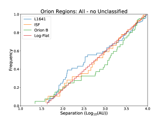
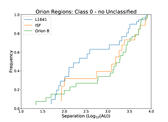
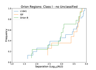
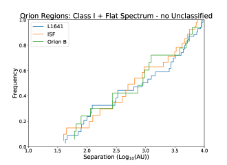
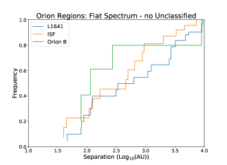
Figure 19: Cumulative separation distributions for the full samples of each region in Orion, and a log-flat distribution is also drawn for comparison for comparison to the full samples of companions. In each protostellar class, all the regions are consistent with being drawn from the same parent distribution, except for Class 0s in L1641 and Orion B.

We compared the probability-weighted cumulative separation distributions for the regions in Figure 19. For the full sample and samples divided by Class, only the Class 0–Class 0 separation distribution in L1641 vs. Orion B regions (separations $<$ 10⁴ au) reject the null hypothesis (that they are drawn from the same parent distribution) with p $<$ 0.01, other classes do not show statistically significant differences between regions. Also, when compared to a log-flat separation distribution, only the Orion B Class 0s are inconsistent with log-flat.

The MFs and CFs for the Orion regions are given in Table 10 Multiplicity and Companion Fractions for Orion Regions, and we show them graphically as a function of protostellar class in Figure 20. For separations of 20 to 10⁴ au, Class 0 protostars in all regions have MFs and CFs that are consistent within their uncertainties. Then, while the MFs of the ISF are systematically higher for more-evolved protostars, the differences are all $<$2$\sigma$ and not definitive. Then the CFs for the more evolved protostars in the ISF, the values are again systematically higher than the other regions, but are not statistically significant with all $<$2$\sigma$. If the full sample of the regions are considered, the difference between the CFs in the ISF and L1641 is $\sim$1.9$\sigma$. Thus, the elevated CFs in the ISF suggest a potential dependence of multiplicity difference between regions, but firm conclusions cannot be drawn.

In the 20 to 10³ au separation range, the MFs and CFs for the Class 0 protostars in the three regions are consistent within the uncertainties. The ISF does have elevated CF values for Class I + Flat Spectrum and Flat Spectrum protostars, but they are just beyond 1$\sigma$. The 20 to 500 au separation range tells a similar story, without statistically significant differences in the MFs and CFs for the different regions. However, there is a hint that the L1641 Class 0 protostars could have a higher MF and CF in this separation range, but the significance of this difference is only sightly greater than 1$\sigma$.

Overall, the only statistically significant difference between regions is found in the Class 0 separation distribution for L1641 vs. Orion B. There are no significant differences in the MFs or CFs between regions, however, the ISF MFs and CFs are systematically higher than those of other regions, providing a hint that it might have a difference. The main difference between the ISF and the other regions is YSO density, being much higher in the ISF, and we discussed in Sections 4.5 and 5.3 that regions with high YSO densities could be more favorable to the formation of multiples.

Figure 1: Graphical demonstration of the construction of multiple systems from our method. The size of the dot is proportional to the luminosity of a component, but this quantity is not used. Our modified nearest neighbor method iteratively searches for companions at progressively larger radii. Once a pair is created, the position is updated to be the average position and additional companions are searched for relative to the average position of the pair. The pairing AB is found first since they have the closest separation, then CD is found later, and finally, the average positions for AB and CD are found to be associated, forming a quadruple system ABCD. Thus, component D is part of the system, despite having a distance greater than 10⁴ au from A, because the average position of CD is within 10⁴ AU of AB. A more conventional approach would assign A to be the primary, creating pairings (A,B), and A,C); (A,D) would be ignored because the separation is greater than 10⁴ au. The S:B:T:Q at the bottom of each panel refers to how we could count the individual continuum sources in our multiplicity statistics (single, binary, triple, quadruple) that comprise this ’system’ depending on what separation range the statistics are being considered.

Table 1: Orion Catalog

Source	Main Source	RA	Decl.	Lbol	Tbol	Class	$\Sigma_{YSO}$	Distance
		(J2000)	(J2000)	(L☉)	(K)		(pc-2)	(pc)
HH270VLA1-A	HH270VLA1	05:51:34.587	+02:56:46.01	7.34	32.00	0	2.2	430.1
HH270VLA1-B	HH270VLA1	05:51:34.600	+02:56:45.88	7.34	32.00	0	2.2	430.1
HH270mms1-B	HH270mms1	05:51:22.632	+02:56:06.80	7.74	72.00	I	2.2	405.7
HH270mms1-A	HH270mms1	05:51:22.717	+02:56:04.98	7.74	72.00	I	2.2	405.7
HH270mms2	HH270mms2	05:51:22.572	+02:55:43.16	4.55	249.00	Flat	2.2	413.3

Note. — Table 1 is published in its entirety in the machine-readable format. A portion is shown here for guidance regarding its form and content.

Table 2: Perseus Catalog

Note. — Table 2 is published in its entirety in the machine-readable format. A portion is shown here for guidance regarding its form and content.

Note. — Classes are provided in abbreviated form: C0 - Class 0, CI - Class I, FS - Flat Spectrum, CII - Class II. Components classified as ‘N’ do not have a classification. Flux ratios are only provided for pairings of single components. The column labeled Prob. corresponds to the probability of the pairing being a true, bound pair and not a line of sight association, based on the YSO surface density. The overall probability of each member may be lower given the multiplicative nature of companion probabilities when pairing two binary (or higher order systems) together.

Note. — Classes are provided in abbreviated form: C0 - Class 0, CI - Class I, FS - Flat Spectrum, CII - Class II. Components classified as None do not have a classification. Flux ratios are only provided for pairings of single components. The column labeled Prob. corresponds to the probability of the pairing being a true, bound pair and not a line of sight association, based on the YSO surface density.

Table 5: Orion and Perseus Multiplicity and Companion Fractions with Probabilities

Note. — Note that the uncertainties are calculated assuming binomial statistics (Wilson score interval) for the MF and CF for CF $<$ 0.5. When the CF $>$ 0.5, we use Poisson uncertainties, see Section 2.4.2. The same uncertainties are applied for all tables in the text.

Table 6: Combined Multiplicity and Companion Fractions with Probabilities

Note. —

Table 7: Multiplicity and Companion Fractions at High and Low YSO Surface Densities

20 - 10000 112:31:0:1:0:0:0:0:0:0:0 0.22${}_{-0.04}^{+0.04}$ 0.24${}_{-0.04}^{+0.04}$ $<$ 30 pc^-2 All - no Unclassified 20 - 10000 112:30:0:1:0:0:0:0:0:0:0 0.22${}_{-0.04}^{+0.04}$ 0.23${}_{-0.04}^{+0.04}$ $<$ 30 pc^-2 Class 0 - (Class 0, Class I, Flat) 20 - 10000 23:12:0:1:0:0:0:0:0:0:0 0.36${}_{-0.09}^{+0.10}$ 0.42${}_{-0.09}^{+0.10}$ $<$ 30 pc^-2 Class I - (Class 0, Class I, Flat) 20 - 10000 56:9:0:0:0:0:0:0:0:0:0 0.14${}_{-0.04}^{+0.06}$ 0.14${}_{-0.04}^{+0.06}$ $<$ 30 pc^-2 Flat - (Class 0, Class I, Flat) 20 - 10000 33:9:0:0:0:0:0:0:0:0:0 0.21${}_{-0.07}^{+0.08}$ 0.21${}_{-0.07}^{+0.08}$ $<$ 30 pc^-2 (Class I, Flat) - (Class 0, Class I, Flat) 20 - 10000 89:18:0:0:0:0:0:0:0:0:0 0.17${}_{-0.04}^{+0.04}$ 0.17${}_{-0.04}^{+0.04}$ $<$ 30 pc^-2 All 20 - 1000 136:21:0:0:0:0:0:0:0:0:0 0.13${}_{-0.03}^{+0.03}$ 0.13${}_{-0.03}^{+0.03}$ $<$ 30 pc^-2 All - no Unclassified 20 - 1000 136:20:0:0:0:0:0:0:0:0:0 0.13${}_{-0.03}^{+0.03}$ 0.13${}_{-0.03}^{+0.03}$ $<$ 30 pc^-2 Class 0 - (Class 0, Class I, Flat) 20 - 1000 32:8:0:0:0:0:0:0:0:0:0 0.20${}_{-0.07}^{+0.08}$ 0.20${}_{-0.07}^{+0.08}$ $<$ 30 pc^-2 Class I - (Class 0, Class I, Flat) 20 - 1000 63:6:0:0:0:0:0:0:0:0:0 0.09${}_{-0.03}^{+0.05}$ 0.09${}_{-0.03}^{+0.05}$ $<$ 30 pc^-2 Flat - (Class 0, Class I, Flat) 20 - 1000 41:6:0:0:0:0:0:0:0:0:0 0.13${}_{-0.05}^{+0.07}$ 0.13${}_{-0.05}^{+0.07}$ $<$ 30 pc^-2 (Class I, Flat) - (Class 0, Class I, Flat) 20 - 1000 104:12:0:0:0:0:0:0:0:0:0 0.10${}_{-0.03}^{+0.04}$ 0.10${}_{-0.03}^{+0.04}$ $<$ 30 pc^-2 All 20 - 500 142:18:0:0:0:0:0:0:0:0:0 0.11${}_{-0.03}^{+0.03}$ 0.11${}_{-0.03}^{+0.03}$ $<$ 30 pc^-2 All - no Unclassified 20 - 500 141:17:0:0:0:0:0:0:0:0:0 0.11${}_{-0.03}^{+0.03}$ 0.11${}_{-0.03}^{+0.03}$ $<$ 30 pc^-2 Class 0 - (Class 0, Class I, Flat) 20 - 500 33:7:0:0:0:0:0:0:0:0:0 0.17${}_{-0.06}^{+0.08}$ 0.17${}_{-0.06}^{+0.08}$ $<$ 30 pc^-2 Class I - (Class 0, Class I, Flat) 20 - 500 65:5:0:0:0:0:0:0:0:0:0 0.07${}_{-0.03}^{+0.05}$ 0.07${}_{-0.03}^{+0.05}$ $<$ 30 pc^-2 Flat - (Class 0, Class I, Flat) 20 - 500 43:5:0:0:0:0:0:0:0:0:0 0.10${}_{-0.04}^{+0.06}$ 0.10${}_{-0.04}^{+0.06}$ $<$ 30 pc^-2 (Class I, Flat) - (Class 0, Class I, Flat) 20 - 500 108:10:0:0:0:0:0:0:0:0:0 0.08${}_{-0.03}^{+0.03}$ 0.08${}_{-0.03}^{+0.03}$ $<$ 30 pc^-2 All 100 - 1000 145:12:0:0:0:0:0:0:0:0:0 0.07${}_{-0.02}^{+0.03}$ 0.07${}_{-0.02}^{+0.03}$ $<$ 30 pc^-2 All - no Unclassified 100 - 1000 145:11:0:0:0:0:0:0:0:0:0 0.07${}_{-0.02}^{+0.03}$ 0.07${}_{-0.02}^{+0.03}$ $<$ 30 pc^-2 Class 0 - (Class 0, Class I, Flat) 100 - 1000 35:5:0:0:0:0:0:0:0:0:0 0.12${}_{-0.05}^{+0.07}$ 0.12${}_{-0.05}^{+0.07}$ $<$ 30 pc^-2 Class I - (Class 0, Class I, Flat) 100 - 1000 66:3:0:0:0:0:0:0:0:0:0 0.04${}_{-0.02}^{+0.04}$ 0.04${}_{-0.02}^{+0.04}$ $<$ 30 pc^-2 Flat - (Class 0, Class I, Flat) 100 - 1000 44:3:0:0:0:0:0:0:0:0:0 0.06${}_{-0.03}^{+0.06}$ 0.06${}_{-0.03}^{+0.06}$ $<$ 30 pc^-2 (Class I, Flat) - (Class 0, Class I, Flat) 100 - 1000 110:6:0:0:0:0:0:0:0:0:0 0.05${}_{-0.02}^{+0.03}$ 0.05${}_{-0.02}^{+0.03}$

Note. —

Table 8: Orion and Perseus Multiplicity and Companion Fractions without Probabilities

Note. — We only provide the 20 to 10⁴ au ranges here because it is the only range affected by the companion probabilities.

Table 9: Combined Multiplicity and Companion Fractions without Probabilities

Note. — We only provide the 20 to 10⁴ au ranges here because it is the only range affected by the companion probabilities.

Table 10: Multiplicity and Companion Fractions for Orion Regions

20 - 10000 57:23:2:0:2:0:0:0:0:1:0:0 0.33${}_{-0.05}^{+0.06}$ 0.52${}_{-0.10}^{+0.10}$ Orion B All - no Unclassified 20 - 10000 52:22:1:0:2:0:0:0:0:1:0:0 0.33${}_{-0.06}^{+0.06}$ 0.53${}_{-0.10}^{+0.10}$ Orion B Class 0 - (Class 0, Class I, Flat) 20 - 10000 22:14:1:0:0:0:0:0:0:1:0:0 0.42${}_{-0.09}^{+0.09}$ 0.66${}_{-0.17}^{+0.17}$ Orion B Class I - (Class 0, Class I, Flat) 20 - 10000 22:5:0:0:2:0:0:0:0:0:0:0 0.24${}_{-0.08}^{+0.11}$ 0.45${}_{-0.11}^{+0.11}$ Orion B Flat - (Class 0, Class I, Flat) 20 - 10000 8:3:0:0:0:0:0:0:0:0:0:0 0.27${}_{-0.15}^{+0.20}$ 0.27${}_{-0.15}^{+0.20}$ Orion B (Class I, Flat) - (Class 0, Class I, Flat) 20 - 10000 30:8:0:0:2:0:0:0:0:0:0:0 0.25${}_{-0.07}^{+0.09}$ 0.40${}_{-0.09}^{+0.09}$ Orion B All 20 - 1000 89:20:0:0:0:0:0:0:0:0:0:0 0.18${}_{-0.04}^{+0.04}$ 0.18${}_{-0.04}^{+0.04}$ Orion B All - no Unclassified 20 - 1000 82:18:0:0:0:0:0:0:0:0:0:0 0.18${}_{-0.04}^{+0.05}$ 0.18${}_{-0.04}^{+0.05}$ Orion B Class 0 - (Class 0, Class I, Flat) 20 - 1000 43:10:0:0:0:0:0:0:0:0:0:0 0.19${}_{-0.06}^{+0.07}$ 0.19${}_{-0.06}^{+0.07}$ Orion B Class I - (Class 0, Class I, Flat) 20 - 1000 30:5:0:0:0:0:0:0:0:0:0:0 0.14${}_{-0.06}^{+0.09}$ 0.14${}_{-0.06}^{+0.09}$ Orion B Flat - (Class 0, Class I, Flat) 20 - 1000 9:3:0:0:0:0:0:0:0:0:0:0 0.25${}_{-0.13}^{+0.18}$ 0.25${}_{-0.13}^{+0.18}$ Orion B (Class I, Flat) - (Class 0, Class I, Flat) 20 - 1000 39:8:0:0:0:0:0:0:0:0:0:0 0.17${}_{-0.06}^{+0.07}$ 0.17${}_{-0.06}^{+0.07}$ Orion B All 20 - 500 101:14:0:0:0:0:0:0:0:0:0:0 0.12${}_{-0.03}^{+0.04}$ 0.12${}_{-0.03}^{+0.04}$ Orion B All - no Unclassified 20 - 500 92:12:0:0:0:0:0:0:0:0:0:0 0.12${}_{-0.03}^{+0.04}$ 0.12${}_{-0.03}^{+0.04}$ Orion B Class 0 - (Class 0, Class I, Flat) 20 - 500 49:6:0:0:0:0:0:0:0:0:0:0 0.11${}_{-0.04}^{+0.06}$ 0.11${}_{-0.04}^{+0.06}$ Orion B Class I - (Class 0, Class I, Flat) 20 - 500 34:3:0:0:0:0:0:0:0:0:0:0 0.08${}_{-0.04}^{+0.07}$ 0.08${}_{-0.04}^{+0.07}$ Orion B Flat - (Class 0, Class I, Flat) 20 - 500 9:3:0:0:0:0:0:0:0:0:0:0 0.25${}_{-0.13}^{+0.18}$ 0.25${}_{-0.13}^{+0.18}$ Orion B (Class I, Flat) - (Class 0, Class I, Flat) 20 - 500 43:6:0:0:0:0:0:0:0:0:0:0 0.12${}_{-0.05}^{+0.07}$ 0.12${}_{-0.05}^{+0.07}$ Orion B All 100 - 1000 95:14:0:0:0:0:0:0:0:0:0:0 0.12${}_{-0.03}^{+0.04}$ 0.12${}_{-0.03}^{+0.04}$ Orion B All - no Unclassified 100 - 1000 88:12:0:0:0:0:0:0:0:0:0:0 0.11${}_{-0.03}^{+0.04}$ 0.11${}_{-0.03}^{+0.04}$ Orion B Class 0 - (Class 0, Class I, Flat) 100 - 1000 46:7:0:0:0:0:0:0:0:0:0:0 0.12${}_{-0.05}^{+0.06}$ 0.12${}_{-0.05}^{+0.06}$ Orion B Class I - (Class 0, Class I, Flat) 100 - 1000 32:3:0:0:0:0:0:0:0:0:0:0 0.08${}_{-0.04}^{+0.07}$ 0.08${}_{-0.04}^{+0.07}$ Orion B Flat - (Class 0, Class I, Flat) 100 - 1000 10:2:0:0:0:0:0:0:0:0:0:0 0.15${}_{-0.10}^{+0.17}$ 0.15${}_{-0.10}^{+0.17}$ Orion B (Class I, Flat) - (Class 0, Class I, Flat) 100 - 1000 42:5:0:0:0:0:0:0:0:0:0:0 0.10${}_{-0.04}^{+0.06}$ 0.10${}_{-0.04}^{+0.06}$ L1641 All 20 - 10000 118:35:5:1:0:0:0:0:0:0:0:0 0.26${}_{-0.04}^{+0.04}$ 0.30${}_{-0.04}^{+0.04}$ L1641 All - no Unclassified 20 - 10000 118:35:5:1:0:0:0:0:0:0:0:0 0.26${}_{-0.04}^{+0.04}$ 0.30${}_{-0.04}^{+0.04}$ L1641 Class 0 - (Class 0, Class I, Flat) 20 - 10000 24:9:4:1:0:0:0:0:0:0:0:0 0.37${}_{-0.09}^{+0.09}$ 0.53${}_{-0.15}^{+0.15}$ L1641 Class I - (Class 0, Class I, Flat) 20 - 10000 52:10:1:0:0:0:0:0:0:0:0:0 0.17${}_{-0.05}^{+0.06}$ 0.19${}_{-0.05}^{+0.06}$ L1641 Flat - (Class 0, Class I, Flat) 20 - 10000 42:16:0:0:0:0:0:0:0:0:0:0 0.28${}_{-0.06}^{+0.07}$ 0.28${}_{-0.06}^{+0.07}$ L1641 (Class I, Flat) - (Class 0, Class I, Flat) 20 - 10000 94:26:1:0:0:0:0:0:0:0:0:0 0.22${}_{-0.04}^{+0.04}$ 0.23${}_{-0.04}^{+0.04}$ L1641 All 20 - 1000 152:26:1:0:0:0:0:0:0:0:0:0 0.15${}_{-0.03}^{+0.03}$ 0.16${}_{-0.03}^{+0.03}$ L1641 All - no Unclassified 20 - 1000 152:26:1:0:0:0:0:0:0:0:0:0 0.15${}_{-0.03}^{+0.03}$ 0.16${}_{-0.03}^{+0.03}$ L1641 Class 0 - (Class 0, Class I, Flat) 20 - 1000 30:10:1:0:0:0:0:0:0:0:0:0 0.27${}_{-0.07}^{+0.09}$ 0.29${}_{-0.08}^{+0.09}$ L1641 Class I - (Class 0, Class I, Flat) 20 - 1000 65:6:0:0:0:0:0:0:0:0:0:0 0.08${}_{-0.03}^{+0.05}$ 0.08${}_{-0.03}^{+0.05}$ L1641 Flat - (Class 0, Class I, Flat) 20 - 1000 57:10:0:0:0:0:0:0:0:0:0:0 0.15${}_{-0.04}^{+0.06}$ 0.15${}_{-0.04}^{+0.06}$ L1641 (Class I, Flat) - (Class 0, Class I, Flat) 20 - 1000 122:16:0:0:0:0:0:0:0:0:0:0 0.12${}_{-0.03}^{+0.03}$ 0.12${}_{-0.03}^{+0.03}$ L1641 All 20 - 500 156:24:1:0:0:0:0:0:0:0:0:0 0.14${}_{-0.03}^{+0.03}$ 0.14${}_{-0.03}^{+0.03}$ L1641 All - no Unclassified 20 - 500 156:24:1:0:0:0:0:0:0:0:0:0 0.14${}_{-0.03}^{+0.03}$ 0.14${}_{-0.03}^{+0.03}$ L1641 Class 0 - (Class 0, Class I, Flat) 20 - 500 30:10:1:0:0:0:0:0:0:0:0:0 0.27${}_{-0.07}^{+0.09}$ 0.29${}_{-0.08}^{+0.09}$ L1641 Class I - (Class 0, Class I, Flat) 20 - 500 67:5:0:0:0:0:0:0:0:0:0:0 0.07${}_{-0.03}^{+0.04}$ 0.07${}_{-0.03}^{+0.04}$ L1641 Flat - (Class 0, Class I, Flat) 20 - 500 59:9:0:0:0:0:0:0:0:0:0:0 0.13${}_{-0.04}^{+0.05}$ 0.13${}_{-0.04}^{+0.05}$ L1641 (Class I, Flat) - (Class 0, Class I, Flat) 20 - 500 126:14:0:0:0:0:0:0:0:0:0:0 0.10${}_{-0.03}^{+0.03}$ 0.10${}_{-0.03}^{+0.03}$ L1641 All 100 - 1000 163:15:1:0:0:0:0:0:0:0:0:0 0.08${}_{-0.02}^{+0.03}$ 0.09${}_{-0.02}^{+0.03}$ L1641 All - no Unclassified 100 - 1000 163:15:1:0:0:0:0:0:0:0:0:0 0.08${}_{-0.02}^{+0.03}$ 0.09${}_{-0.02}^{+0.03}$ L1641 Class 0 - (Class 0, Class I, Flat) 100 - 1000 35:5:1:0:0:0:0:0:0:0:0:0 0.13${}_{-0.05}^{+0.07}$ 0.15${}_{-0.05}^{+0.07}$ L1641 Class I - (Class 0, Class I, Flat) 100 - 1000 67:4:0:0:0:0:0:0:0:0:0:0 0.05${}_{-0.03}^{+0.04}$ 0.05${}_{-0.03}^{+0.04}$ L1641 Flat - (Class 0, Class I, Flat) 100 - 1000 61:6:0:0:0:0:0:0:0:0:0:0 0.08${}_{-0.03}^{+0.05}$ 0.08${}_{-0.03}^{+0.05}$ L1641 (Class I, Flat) - (Class 0, Class I, Flat) 100 - 1000 128:10:0:0:0:0:0:0:0:0:0:0 0.07${}_{-0.02}^{+0.03}$ 0.07${}_{-0.02}^{+0.03}$

Note. —

References

- Adams et al. (1989) Adams, F. C., Ruden, S. P., & Shu, F. H. 1989, ApJ, 347, 959, doi: 10.1086/168187
- Akeson et al. (2019) Akeson, R. L., Jensen, E. L. N., Carpenter, J., et al. 2019, ApJ, 872, 158, doi: 10.3847/1538-4357/aaff6a
- Allen et al. (2008) Allen, T. S., Pipher, J. L., Gutermuth, R. A., et al. 2008, ApJ, 675, 491, doi: 10.1086/525241
- Alves et al. (2019) Alves, F. O., Caselli, P., Girart, J. M., et al. 2019, Science, 366, 90, doi: 10.1126/science.aaw3491
- André et al. (1993) André, P., Ward-Thompson, D., & Barsony, M. 1993, ApJ, 406, 122, doi: 10.1086/172425
- Ansdell et al. (2016) Ansdell, M., Williams, J. P., van der Marel, N., et al. 2016, ApJ, 828, 46, doi: 10.3847/0004-637X/828/1/46
- Artymowicz & Lubow (1994) Artymowicz, P., & Lubow, S. H. 1994, ApJ, 421, 651, doi: 10.1086/173679
- Astropy Collaboration et al. (2018) Astropy Collaboration, Price-Whelan, A. M., Sipőcz, B. M., et al. 2018, The Astropy Project: Building an Open-science Project and Status of the v2.0 Core Package, doi: 10.3847/1538-3881/aabc4f
- Bate (2012) Bate, M. R. 2012, MNRAS, 419, 3115, doi: 10.1111/j.1365-2966.2011.19955.x
- Bate et al. (2002) Bate, M. R., Bonnell, I. A., & Bromm, V. 2002, MNRAS, 336, 705, doi: 10.1046/j.1365-8711.2002.05775.x
- Benson & Myers (1989) Benson, P. J., & Myers, P. C. 1989, ApJS, 71, 89, doi: 10.1086/191365
- Bergin & Tafalla (2007) Bergin, E. A., & Tafalla, M. 2007, ARA&A, 45, 339, doi: 10.1146/annurev.astro.45.071206.100404
- Branch (1976) Branch, D. 1976, ApJ, 210, 392, doi: 10.1086/154841
- Brandeker et al. (2006) Brandeker, A., Jayawardhana, R., Khavari, P., Haisch, Karl E., J., & Mardones, D. 2006, ApJ, 652, 1572, doi: 10.1086/508483
- Carpenter (2000) Carpenter, J. M. 2000, AJ, 120, 3139, doi: 10.1086/316845
- Carrasco-González et al. (2012) Carrasco-González, C., Osorio, M., Anglada, G., et al. 2012, ApJ, 746, 71, doi: 10.1088/0004-637X/746/1/71
- Casertano & Hut (1985) Casertano, S., & Hut, P. 1985, ApJ, 298, 80, doi: 10.1086/163589
- Chen et al. (2013) Chen, X., Arce, H. G., Zhang, Q., et al. 2013, ApJ, 768, 110, doi: 10.1088/0004-637X/768/2/110
- Connelley et al. (2008) Connelley, M. S., Reipurth, B., & Tokunaga, A. T. 2008, AJ, 135, 2526, doi: 10.1088/0004-6256/135/6/2526
- Cournoyer-Cloutier et al. (2021) Cournoyer-Cloutier, C., Tran, A., Lewis, S., et al. 2021, MNRAS, 501, 4464, doi: 10.1093/mnras/staa3902
- De Furio et al. (2019) De Furio, M., Reiter, M., Meyer, M. R., et al. 2019, ApJ, 886, 95, doi: 10.3847/1538-4357/ab4ae3
- Duchêne et al. (2007) Duchêne, G., Bontemps, S., Bouvier, J., et al. 2007, A&A, 476, 229, doi: 10.1051/0004-6361:20077270
- Duchêne et al. (2004) Duchêne, G., Bouvier, J., Bontemps, S., André, P., & Motte, F. 2004, A&A, 427, 651, doi: 10.1051/0004-6361:20041209
- Duchêne & Kraus (2013) Duchêne, G., & Kraus, A. 2013, ARA&A, 51, 269, doi: 10.1146/annurev-astro-081710-102602
- Duchêne et al. (2018) Duchêne, G., Lacour, S., Moraux, E., Goodwin, S., & Bouvier, J. 2018, MNRAS, 478, 1825, doi: 10.1093/mnras/sty1180
- Dunham et al. (2014) Dunham, M. M., Stutz, A. M., Allen, L. E., et al. 2014, Protostars and Planets VI, 195, doi: 10.2458/azu_uapress_9780816531240-ch009
- Encalada et al. (2021) Encalada, F. J., Looney, L. W., Tobin, J. J., et al. 2021, ApJ, 913, 149, doi: 10.3847/1538-4357/abf4fd
- Enoch et al. (2009) Enoch, M. L., Evans, N. J., Sargent, A. I., & Glenn, J. 2009, ApJ, 692, 973, doi: 10.1088/0004-637X/692/2/973
- Fabrycky & Tremaine (2007) Fabrycky, D., & Tremaine, S. 2007, ApJ, 669, 1298, doi: 10.1086/521702
- Fischer et al. (2010) Fischer, W. J., Megeath, S. T., Ali, B., et al. 2010, A&A, 518, L122, doi: 10.1051/0004-6361/201014636
- Fischer et al. (2017) Fischer, W. J., Megeath, S. T., Furlan, E., et al. 2017, ApJ, 840, 69, doi: 10.3847/1538-4357/aa6d69
- Fisher (2004) Fisher, R. T. 2004, ApJ, 600, 769
- Furlan et al. (2016) Furlan, E., Fischer, W. J., Ali, B., et al. 2016, ApJS, 224, 5, doi: 10.3847/0067-0049/224/1/5
- Greenfield et al. (2013) Greenfield, P., Robitaille, T., Tollerud, E., et al. 2013. http://ascl.net/1304.002
- Grossman et al. (1987) Grossman, E. N., Masson, C. R., Sargent, A. I., et al. 1987, ApJ, 320, 356, doi: 10.1086/165549
- Gutermuth et al. (2005) Gutermuth, R. A., Megeath, S. T., Pipher, J. L., et al. 2005, ApJ, 632, 397, doi: 10.1086/432460
- Gutermuth et al. (2011) Gutermuth, R. A., Pipher, J. L., Megeath, S. T., et al. 2011, ApJ, 739, 84, doi: 10.1088/0004-637X/739/2/84
- Habel et al. (2021) Habel, N. M., Megeath, S. T., Booker, J. J., et al. 2021, ApJ, 911, 153, doi: 10.3847/1538-4357/abded8
- Harris et al. (2012) Harris, R. J., Andrews, S. M., Wilner, D. J., & Kraus, A. L. 2012, ApJ, 751, 115, doi: 10.1088/0004-637X/751/2/115
- Hsu et al. (2013) Hsu, W.-H., Hartmann, L., Allen, L., et al. 2013, ApJ, 764, 114, doi: 10.1088/0004-637X/764/2/114
- Karnath et al. (2020) Karnath, N., Megeath, S. T., Tobin, J. J., et al. 2020, ApJ, 890, 129, doi: 10.3847/1538-4357/ab659e
- King et al. (2012) King, R. R., Parker, R. J., Patience, J., & Goodwin, S. P. 2012, MNRAS, 421, 2025, doi: 10.1111/j.1365-2966.2012.20437.x
- Kirk et al. (2017) Kirk, H., Friesen, R. K., Pineda, J. E., et al. 2017, ApJ, 846, 144, doi: 10.3847/1538-4357/aa8631
- Kounkel et al. (2016) Kounkel, M., Megeath, S. T., Poteet, C. A., Fischer, W. J., & Hartmann, L. 2016, ApJ, 821, 52, doi: 10.3847/0004-637X/821/1/52
- Kounkel et al. (2017) Kounkel, M., Hartmann, L., Loinard, L., et al. 2017, ApJ, 834, 142, doi: 10.3847/1538-4357/834/2/142
- Kounkel et al. (2018) Kounkel, M., Covey, K., Suárez, G., et al. 2018, AJ, 156, 84, doi: 10.3847/1538-3881/aad1f1
- Kounkel et al. (2019) Kounkel, M., Covey, K., Moe, M., et al. 2019, AJ, 157, 196, doi: 10.3847/1538-3881/ab13b1
- Kouwenhoven et al. (2007) Kouwenhoven, M. B. N., Brown, A. G. A., Portegies Zwart, S. F., & Kaper, L. 2007, A&A, 474, 77, doi: 10.1051/0004-6361:20077719
- Kratter & Lodato (2016) Kratter, K., & Lodato, G. 2016, ARA&A, 54, 271, doi: 10.1146/annurev-astro-081915-023307
- Kratter et al. (2010) Kratter, K. M., Matzner, C. D., Krumholz, M. R., & Klein, R. I. 2010, ApJ, 708, 1585, doi: 10.1088/0004-637X/708/2/1585
- Kraus et al. (2011) Kraus, A. L., Ireland, M. J., Martinache, F., & Hillenbrand, L. A. 2011, ApJ, 731, 8, doi: 10.1088/0004-637X/731/1/8
- Kristensen & Dunham (2018) Kristensen, L. E., & Dunham, M. M. 2018, A&A, 618, A158, doi: 10.1051/0004-6361/201731584
- Kroupa (1995) Kroupa, P. 1995, MNRAS, 277, 1507, doi: 10.1093/mnras/277.4.1507
- Krumholz et al. (2016) Krumholz, M. R., Myers, A. T., Klein, R. I., & McKee, C. F. 2016, MNRAS, 460, 3272, doi: 10.1093/mnras/stw1236
- Kuiper (1935) Kuiper, G. P. 1935, PASP, 47, 121, doi: 10.1086/124573
- Lada (1987) Lada, C. J. 1987, in IAU Symp. 115: Star Forming Regions, ed. M. Peimbert & J. Jugaku, 1–17
- Lane et al. (2016) Lane, J., Kirk, H., Johnstone, D., et al. 2016, ApJ, 833, 44, doi: 10.3847/1538-4357/833/1/44
- Lee et al. (2019) Lee, A. T., Offner, S. S. R., Kratter, K. M., Smullen, R. A., & Li, P. S. 2019, ApJ, 887, 232, doi: 10.3847/1538-4357/ab584b
- Lee et al. (2016) Lee, K. I., Dunham, M. M., Myers, P. C., et al. 2016, ApJ, 820, L2, doi: 10.3847/2041-8205/820/1/L2
- Li et al. (2018) Li, P. S., Klein, R. I., & McKee, C. F. 2018, MNRAS, 473, 4220, doi: 10.1093/mnras/stx2611
- Looney et al. (2000) Looney, L. W., Mundy, L. G., & Welch, W. J. 2000, ApJ, 529, 477, doi: 10.1086/308239
- Machida et al. (2008) Machida, M. N., Tomisaka, K., Matsumoto, T., & Inutsuka, S. 2008, ApJ, 677, 327, doi: 10.1086/529133
- Manara et al. (2019) Manara, C. F., Tazzari, M., Long, F., et al. 2019, A&A, 628, A95, doi: 10.1051/0004-6361/201935964
- Maureira et al. (2020) Maureira, M. J., Pineda, J. E., Segura-Cox, D. M., et al. 2020, ApJ, 897, 59, doi: 10.3847/1538-4357/ab960b
- Maury et al. (2010) Maury, A. J., André, P., Hennebelle, P., et al. 2010, A&A, 512, A40, doi: 10.1051/0004-6361/200913492
- McClure et al. (2010) McClure, M. K., Furlan, E., Manoj, P., et al. 2010, ApJS, 188, 75, doi: 10.1088/0067-0049/188/1/75
- McMullin et al. (2007) McMullin, J. P., Waters, B., Schiebel, D., Young, W., & Golap, K. 2007, in Astronomical Society of the Pacific Conference Series, Vol. 376, Astronomical Data Analysis Software and Systems XVI, ed. R. A. Shaw, F. Hill, & D. J. Bell, 127
- Megeath et al. (2012) Megeath, S. T., Gutermuth, R., Muzerolle, J., et al. 2012, AJ, 144, 192, doi: 10.1088/0004-6256/144/6/192
- Megeath et al. (2016) —. 2016, AJ, 151, 5, doi: 10.3847/0004-6256/151/1/5
- Moe & Di Stefano (2017) Moe, M., & Di Stefano, R. 2017, ApJS, 230, 15, doi: 10.3847/1538-4365/aa6fb6
- Moe & Kratter (2018) Moe, M., & Kratter, K. M. 2018, ApJ, 854, 44, doi: 10.3847/1538-4357/aaa6d2
- Moeckel & Clarke (2011) Moeckel, N., & Clarke, C. J. 2011, MNRAS, 415, 1179, doi: 10.1111/j.1365-2966.2011.18731.x
- Murillo et al. (2016) Murillo, N. M., van Dishoeck, E. F., Tobin, J. J., & Fedele, D. 2016, A&A, 592, A56, doi: 10.1051/0004-6361/201628247
- Muzerolle et al. (2013) Muzerolle, J., Furlan, E., Flaherty, K., Balog, Z., & Gutermuth, R. 2013, Nature, 493, 378, doi: 10.1038/nature11746
- Offner & Arce (2014) Offner, S. S. R., & Arce, H. G. 2014, ApJ, 784, 61, doi: 10.1088/0004-637X/784/1/61
- Offner et al. (2016) Offner, S. S. R., Dunham, M. M., Lee, K. I., Arce, H. G., & Fielding, D. B. 2016, ApJ, 827, L11, doi: 10.3847/2041-8205/827/1/L11
- Offner et al. (2010) Offner, S. S. R., Kratter, K. M., Matzner, C. D., Krumholz, M. R., & Klein, R. I. 2010, ApJ, 725, 1485, doi: 10.1088/0004-637X/725/2/1485
- Öpik (1924) Öpik, E. 1924, Publications of the Tartu Astrofizica Observatory, 25, 1
- Orkisz et al. (2019) Orkisz, J. H., Peretto, N., Pety, J., et al. 2019, A&A, 624, A113, doi: 10.1051/0004-6361/201833410
- Ortiz-León et al. (2017) Ortiz-León, G. N., Loinard, L., Kounkel, M. A., et al. 2017, ApJ, 834, 141, doi: 10.3847/1538-4357/834/2/141
- Ortiz-León et al. (2018) Ortiz-León, G. N., Loinard, L., Dzib, S. A., et al. 2018, ApJ, 865, 73, doi: 10.3847/1538-4357/aada49
- Osorio et al. (2017) Osorio, M., Díaz-Rodríguez, A. K., Anglada, G., et al. 2017, ApJ, 840, 36, doi: 10.3847/1538-4357/aa6975
- Padoan & Nordlund (2002) Padoan, P., & Nordlund, Å. 2002, ApJ, 576, 870, doi: 10.1086/341790
- Pokhrel et al. (2020) Pokhrel, R., Gutermuth, R. A., Betti, S. K., et al. 2020, ApJ, 896, 60, doi: 10.3847/1538-4357/ab92a2
- Raghavan et al. (2010) Raghavan, D., McAlister, H. A., Henry, T. J., et al. 2010, ApJS, 190, 1, doi: 10.1088/0067-0049/190/1/1
- Reipurth et al. (2007) Reipurth, B., Guimarães, M. M., Connelley, M. S., & Bally, J. 2007, AJ, 134, 2272, doi: 10.1086/523596
- Reipurth & Mikkola (2012) Reipurth, B., & Mikkola, S. 2012, Nature, 492, 221, doi: 10.1038/nature11662
- Reipurth et al. (2002) Reipurth, B., Rodríguez, L. F., Anglada, G., & Bally, J. 2002, AJ, 124, 1045, doi: 10.1086/341172
- Reipurth & Zinnecker (1993) Reipurth, B., & Zinnecker, H. 1993, A&A, 278, 81
- Ren & Li (2016) Ren, Z., & Li, D. 2016, ApJ, 824, 52, doi: 10.3847/0004-637X/824/1/52
- Reynolds et al. (2021) Reynolds, N. K., Tobin, J. J., Sheehan, P., et al. 2021, ApJ, 907, L10, doi: 10.3847/2041-8213/abcc02
- Robitaille & Bressert (2012) Robitaille, T., & Bressert, E. 2012, APLpy: Astronomical Plotting Library in Python, Astrophysics Source Code Library. http://ascl.net/1208.017
- Sadavoy & Stahler (2017) Sadavoy, S. I., & Stahler, S. W. 2017, MNRAS, 469, 3881, doi: 10.1093/mnras/stx1061
- Sadavoy et al. (2014) Sadavoy, S. I., Di Francesco, J., André, P., et al. 2014, ApJ, 787, L18, doi: 10.1088/2041-8205/787/2/L18
- Sana & Evans (2011) Sana, H., & Evans, C. J. 2011, in IAU Symposium, Vol. 272, IAU Symposium, ed. C. Neiner, G. Wade, G. Meynet, & G. Peters, 474–485, doi: 10.1017/S1743921311011124
- Segura-Cox et al. (2018) Segura-Cox, D. M., Looney, L. W., Tobin, J. J., et al. 2018, ApJ, 866, 161, doi: 10.3847/1538-4357/aaddf3
- Sheehan et al. (2020) Sheehan, P. D., Tobin, J. J., Federman, S., Megeath, S. T., & Looney, L. W. 2020, ApJ, 902, 141, doi: 10.3847/1538-4357/abbad5
- Skrutskie et al. (2006) Skrutskie, M. F., Cutri, R. M., Stiening, R., et al. 2006, AJ, 131, 1163, doi: 10.1086/498708
- Stanke et al. (2000) Stanke, T., McCaughrean, M. J., & Zinnecker, H. 2000, A&A, 355, 639. https://arxiv.org/abs/astro-ph/0001133
- Stutz & Kainulainen (2015) Stutz, A. M., & Kainulainen, J. 2015, A&A, 577, L6, doi: 10.1051/0004-6361/201526243
- Stutz et al. (2013) Stutz, A. M., Tobin, J. J., Stanke, T., et al. 2013, ApJ, 767, 36, doi: 10.1088/0004-637X/767/1/36
- Teixeira et al. (2016) Teixeira, P. S., Takahashi, S., Zapata, L. A., & Ho, P. T. P. 2016, A&A, 587, A47, doi: 10.1051/0004-6361/201526807
- Tobin et al. (2015) Tobin, J. J., Looney, L. W., Wilner, D. J., et al. 2015, ApJ, 805, 125, doi: 10.1088/0004-637X/805/2/125
- Tobin et al. (2016a) Tobin, J. J., Looney, L. W., Li, Z.-Y., et al. 2016a, ApJ, 818, 73, doi: 10.3847/0004-637X/818/1/73
- Tobin et al. (2016b) Tobin, J. J., Kratter, K. M., Persson, M. V., et al. 2016b, Nature, 538, 483, doi: 10.1038/nature20094
- Tobin et al. (2018) Tobin, J. J., Looney, L. W., Li, Z.-Y., et al. 2018, ApJ, 867, 43, doi: 10.3847/1538-4357/aae1f7
- Tobin et al. (2019) Tobin, J. J., Megeath, S. T., van’t Hoff, M., et al. 2019, ApJ, 886, 6, doi: 10.3847/1538-4357/ab498f
- Tobin et al. (2020) Tobin, J. J., Sheehan, P. D., Megeath, S. T., et al. 2020, ApJ, 890, 130, doi: 10.3847/1538-4357/ab6f64
- Tohline (2002) Tohline, J. E. 2002, ARA&A, 40, 349, doi: 10.1146/annurev.astro.40.060401.093810
- Tokovinin & Moe (2020) Tokovinin, A., & Moe, M. 2020, MNRAS, 491, 5158, doi: 10.1093/mnras/stz3299
- van Kempen et al. (2016) van Kempen, T. A., Hogerheijde, M. R., van Dishoeck, E. F., et al. 2016, A&A, 587, A17, doi: 10.1051/0004-6361/201424725
- van Terwisga et al. (2020) van Terwisga, S. E., van Dishoeck, E. F., Mann, R. K., et al. 2020, A&A, 640, A27, doi: 10.1051/0004-6361/201937403
- Viana Almeida et al. (2012) Viana Almeida, P., Melo, C., Santos, N. C., et al. 2012, A&A, 539, A62, doi: 10.1051/0004-6361/201117703
- Ward-Duong et al. (2015) Ward-Duong, K., Patience, J., De Rosa, R. J., et al. 2015, MNRAS, 449, 2618, doi: 10.1093/mnras/stv384
- Wilson (1927) Wilson, E. B. 1927, Journal of the American Statistical Association, 22, 209, doi: 10.1080/01621459.1927.10502953
- Winters et al. (2019) Winters, J. G., Henry, T. J., Jao, W.-C., et al. 2019, AJ, 157, 216, doi: 10.3847/1538-3881/ab05dc
- Yıldız et al. (2012) Yıldız, U. A., Kristensen, L. E., van Dishoeck, E. F., et al. 2012, A&A, 542, A86, doi: 10.1051/0004-6361/201118368