On the evaluation of the

Appell $F_{2}$ double hypergeometric function

B. Ananthanarayan^a∗, Souvik Bera^a†, S. Friot^b,c‡, O. Marichev^d⋄ and Tanay Pathak^a⋆
a Centre for High Energy Physics, Indian Institute of Science,

Bangalore-560012, Karnataka, India

^b Université Paris-Saclay, CNRS/IN2P3, IJCLab, 91405 Orsay, France

^c Univ Lyon, Univ Claude Bernard Lyon 1, CNRS/IN2P3,

IP2I Lyon, UMR 5822, F-69622, Villeurbanne, France

^d Wolfram Research, Inc., 100 Trade Center Drive, Champaign, IL 61820-7237, USA

The transformation theory of the Appell $F_{2}(a,b_{1},b_{2};c_{1},c_{2};x,y)$ double hypergeometric function is used to obtain a set of series representations of $F_{2}$ which provide an efficient way to evaluate $F_{2}$ for real values of its arguments $x$ and $y$ and generic complex values of its parameters $a,b_{1},b_{2},c_{1}$ and $c_{2}$ (i.e. in the nonlogarithmic case). This study rests on a classical approach where the usual double series representation of $F_{2}$ and other double hypergeometric series that appear in the intermediate steps of the calculations are written as infinite sums of one variable hypergeometric series, such as the Gauss ${}_{2}F_{1}$ or the ${}_{3}F_{2}$, various linear transformations of the latter being then applied to derive known and new formulas. Using the three well-known Euler transformations of $F_{2}$ on these results allows us to obtain a total of 44 series which form the basis of the Mathematica package AppellF2, dedicated to the evaluation of $F_{2}$. A brief description of the package and of the numerical analysis that we have performed to test it are also presented.

$\ast$ anant@iisc.ac.in

$\dagger$ souvikbera@iisc.ac.in

$\ddagger$ samuel.friot@universite-paris-saclay.fr

$\diamond$ oleg@wolfram.com

$\star$ tanaypathak@iisc.ac.in

1 Introduction

The study of multiple hypergeometric functions, which appear in many domains of the physical and mathematical sciences, mainly began in 1880 with Appell who introduced the famous four double hypergeometric functions $F_{1},F_{2},F_{3}$ and $F_{4}$ that carry his name and are generalizations of the Gauss hypergeometric ${}_{2}F_{1}$ function. Since then, a huge development of this field, by the extensive study of many classes of multiple hypergeometric functions, led it to become a classical branch of mathematics. On the other hand, the implementation of the automatic evaluation of these multivariable functions in softwares dedicated to mathematics is a field of investigations which is nearly virgin. For instance, in Mathematica [1] only the Appell $F_{1}$ has been coded, and in Maple [2], the four Appell functions are the only hypergeometric functions of more than one variable that are in-built functions (since 2017).

One can point out several difficulties that may be at the origin of such a lack. One of them is that the integral representations of multiple hypergeometric functions are not always known and, when known, they are in general not valid for all values of the parameters of the hypergeometric functions that they represent. They can also be hard to compute numerically.

An alternative way to handle multiple hypergeometric functions is to consider their series representations and, using transformation theory [3, 4], to obtain other series representations converging in other regions of the space of their variables, giving thereby analytic continuations of the starting point series. One interest of this approach is that the convergence properties of multiple hypergeometric series are independent of the values of their parameters (exceptional values of the parameters being excluded). Thus, one can use these series representations for numerical purpose when the Euler integral representations (or other integral representations) are not defined, or are unknown. Another advantage is that it is often easier to numerically compute series than integrals. However, one has to point out that beyond the case of double series, the convergence regions of multivariable hypergeometric series can be difficult to obtain. Moreover, to our knowledge, there is no systematic approach to derive transformations of these series that can collectively provide an evaluation of the corresponding multiple hypergeometric functions for all the possible values of their variables.

In what concerns the analytic continuation of multiple hypergeometric series, a recent and important progress can be mentioned. In [5], two of the authors of the present paper have developed, with other collaborators, a very efficient and systematic approach to analytically compute multiple Mellin-Barnes (MB) integrals. It is well-known that MB integrals are intimately linked to hypergeometric functions [6, 7, 8]. Multiple MB integrals are in fact one of the possible starting points for the study of hypergeometric functions of several variables [9]. Therefore, by the study of appropriate classes of multiple MB integrals, the method of [5] opens promising horizons in hypergeometric functions theory and, in particular, for the determination of the analytic continuations of many classes of hypergeometric series, whatever the number of their variables is, in terms of others multivariable hypergeometric series. Obviously, a large number of applications can follow in physics, as already shown in the recent works [10] and [11] in the context of the study of Feynman integrals in quantum field theory.

Although many new results can be obtained from the powerful method developed in [5], it cannot, alone, fully solve the difficult problem of finding the relevant set of transformations of a multiple hypergeometric function that will allow to evaluate it for all values of its variables. Indeed, we have mentioned above some possible difficulties in the derivation of the convergence regions of the new series representations obtained from transformation theory. But another problem can be that some hypergeometric functions of several variables do not have an obvious MB representation. Moreover, even if the latter can be obtained, the evaluation of the MB integral in general shows that “white regions” (as called in [12]) appear in the multivariable space, where none of the obtained analytic continuations converges. Although some manipulations of the MB integral can lead to transformations and, thus, to other formulas (in addition to those obtained by a direct application of [5]), it is not clear that a systematic approach for these manipulations can be found. Therefore, in order to fully solve the problem of evaluating multivariable hypergeometric functions for all values of their variables, it may be necessary to rely on alternative approaches, in order to complete the results obtained from the MB approach.

A well-known example of such a situation in the context of quantum field theory involves the triple hypergeometric function of Lauricella $F_{C}$ type [13]. This particular function, which is the natural extension of the Appell $F_{4}$ double hypergeometric function, appears when one computes the two-loop sunset Feynman integral with four mass scales. It is easy to conclude from [13] that the analytic continuations of the $F_{C}$ triple series, derived from the Mellin-Barnes representation of the $F_{C}$ function, give access to a restricted region of its three variables space. Therefore, in order to obtain analytic expressions for the sunset outside this region, some transformations of the $F_{C}$ Lauricella series have been obtained in [14], using an alternative method. This method, which uses quadratic transformations of the Gauss ${}_{2}F_{1}$ hypergeometric series as intermediate steps in the derivation of new series representations for $F_{4}$ [15] (and, as a by product, for $F_{C}$) can be seen as an extension of a classical work of Olsson [16] which focused on the question of the analytic contination of the Appell $F_{1}$ series and of its $F_{D}$ multivariable generalisation, using linear transformations of ${}_{2}F_{1}$. The approach of [14, 15] can however not give the full answer to the problem of finding series representations that can be used to evaluate the $F_{C}$ function for all values of its variables.

Our aim in the present work is to explore Olsson’s approach more systematically, taking the simpler case of the Appell $F_{2}$ double hypergeometric function as a theoretical laboratory, having in mind, among others, to come back at a later stage to the case of the Lauricella $F_{C}$ and other multivariable hypergeometric functions.

The Appell $F_{2}$ double hypergeometric function is not an arbitrary choice, it has indeed a particular place in the set of the 14 complete double hypergeometric functions of order 2, which consist of the four Appell functions $F_{i},(i=1,...,4)$ and the ten Horn functions $G_{i},(i=1,..,3)$ and $H_{i},(i=1,...,7)$. Indeed, it has been noticed in [17] that, with the exception of $F_{4},H_{1}$ and $H_{5}$, the Appell $F_{2}$ function can be related to any of the other Horn and Appell functions. These links can be obtained from the transformation theory of $F_{2}$ and are summarized in Chapter 5 of [3]. Hence, in the present work, by studying the linear transformations of $F_{2}$ and by building the AppellF2 Mathematica package based on the obtained formulas and dedicated to its numerical evaluation, we provide the basis of a future Mathematica package for the evaluation of all the double series above [19], with the exception of $F_{4}$, $H_{1}$ and $H_{5}$. These three lacking series will be considered separately in subsequent publications.

The plan of the paper is as follows. In Section 2, we briefly list some of the well-known properties of the Appell $F_{2}$ function. In Section 3, we perform a first analytic continuation study of the Appell $F_{2}$ series from the Mellin-Barnes approach [5], which is completed in Section 4 following Olsson’s method. This analysis, which yields 11 series representations of $F_{2}$, can be extended with the use of the three Euler transformations of $F_{2}$, allowing us to obtain a total set of 43 linear transformations of $F_{2}$, out of which 17 are needed, in addition to the usual series definition of $F_{2}$, to cover the $(x,y)$ space of the $F_{2}$ variables for real values of the latter, with the exception of a few points. This subset of 18 series representations of $F_{2}$ are recapitulated in the appendix along with the figures showing their corresponding regions of convergence for real values of the arguments. The mathematical expressions and convergence regions of the remaining 26 series can be obtained from our AppellF2 package. These additional series increase the efficiency of the package from the convergence perspective by enlarging the possible ways to compute $F_{2}$. Section 5 is dedicated to the description of the AppellF2 package and its numerical tests, which are followed by the conclusions and the appendix.

2 The Appell $F_{2}$ function

The Appell $F_{2}$ double hypergeometric series is defined as [6]

$$F_{2}(a,b_{1},b_{2};c_{1},c_{2};x,y)=\sum_{m=0}^{\infty}\sum_{n=0}^{\infty}\frac{(a)_{m+n}(b_{1})_{m}(b_{2})_{n}}{(c_{1})_{m}(c_{2})_{n}m!n!}x^{m}y^{n}$$ (1)

where $(a)_{m}=\frac{\Gamma(a+m)}{\Gamma(a)}$ is the Pochhammer symbol. The series in the RHS of Eq.(1) converges for $|x|+|y|<1$ which is the region, shown in Fig. 1 (Left),

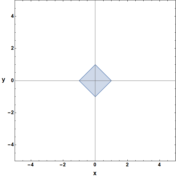
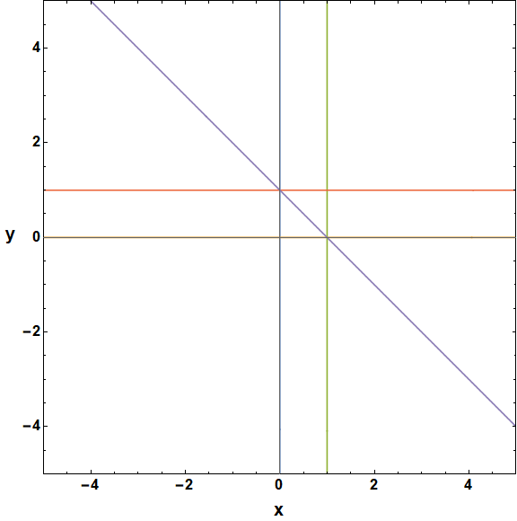
Figure 1: Left: Region of convergence (ROC) of the Appell $F_{2}$ series for real values of its arguments $x$ and $y$. Right: Singular curves of Eq.(7).

where the $F_{2}$ series coincides with the Appell $F_{2}$ function. Outside of this region, the Appell $F_{2}$ function can be defined by the integral representation of the Euler type

$$F_{2}(a,b_{1},b_{2};c_{1},c_{2};x,y)=$$

$$\frac{\Gamma(c_{1})\Gamma(c_{2})}{\Gamma(b_{1})\Gamma(b_{2})\Gamma(c_{1}-b_{1})\Gamma(c_{2}-b_{2})}\int_{0}^{1}du\int_{0}^{1}\ dv\ u^{b_{1}-1}v^{b_{2}-1}(1-u)^{c_{1}-b_{1}-1}(1-v)^{c_{2}-b_{2}-1}(1-ux-vy)^{-a}$$ (2)

subject to the constraints that $\text{Re}(b_{1}),\text{Re}(b_{2}),\text{Re}(c_{1}-b_{1})$ and $\text{Re}(c_{2}-b_{2})$ are positive numbers, or by

$$F_{2}(a,b_{1},b_{2};c_{1},c_{2};x,y)=\frac{\Gamma(c_{2})}{\Gamma(b_{2})\Gamma(c_{2}-b_{2})}\int_{0}^{1}dvv^{b_{2}-1}(1-vy)^{-a}(1-v)^{-b_{2}+c_{2}-1}{}_{2}F_{1}\left(a,b_{1};c_{1};\frac{x}{1-vy}\right)$$ (3)

Another well-known integral representation of $F_{2}$ is of the Mellin-Barnes type

$$F_{2}(a,b_{1},b_{2}; c_{1},c_{2};x,y)=$$

$$\frac{\Gamma(c_{1})\Gamma(c_{2})}{\Gamma(a)\Gamma(b_{1})\Gamma(b_{2})}\int_{-i\infty}^{+i\infty}ds\int_{-i\infty}^{+i\infty}dt\ (-x)^{s}(-y)^{t}\Gamma(-s)\Gamma(-t)\frac{\Gamma(a+s+t)\Gamma(b_{1}+s)\Gamma(b_{2}+t)}{\Gamma(c_{1}+s)\Gamma(c_{2}+t)}$$ (4)

where the integration contours are such that they separate the poles of $\Gamma(-s)$ and $\Gamma(-t)$ from those of $\Gamma(a+s+t)$, $\Gamma(b_{1}+s)$ and $\Gamma(b_{2}+t)$.

$F_{2}$ has the following symmetry

$$F_{2}(a,b_{1},b_{2};c_{1},c_{2};x,y)=F_{2}(a,b_{2},b_{1};c_{2},c_{1};y,x)$$ (5)

and from suitable changes of variables in Eq.(2), one can obtain its well-known Euler transformations [6]

$$F_{2}(a,b_{1},b_{2};c_{1},c_{2};x,y) =(1-x)^{-a}F_{2}\left(a,c_{1}-b_{1},b_{2};c_{1},c_{2};\frac{x}{x-1},\frac{y}{1-x}\right)$$

$$=(1-y)^{-a}F_{2}\left(a,b_{1},c_{2}-b_{2};c_{1},c_{2};\frac{x}{1-y},\frac{y}{y-1}\right)$$

$$=(1-x-y)^{-a}F_{2}\left(a,c_{1}-b_{1},c_{2}-b_{2};c_{1},c_{2};\frac{x}{x+y-1},\frac{y}{x+y-1}\right)$$ (6)

which will be useful in the following.

The system of partial differential equations satisfied by $F_{2}$ is given by [6]

$$x(1-x)r-xys+[c_{1}-(a+b_{1}+1)x]p-b_{1}yq-ab_{1}z=0$$

$$y(1-y)t-xys+[c_{2}-(a+b_{2}+1)y]q-b_{2}xp-ab_{2}z=0$$ (7)

where $r=z_{xx}$, $t=z_{yy}$, $s=z_{xy}$, $p=z_{x}$, $q=z_{y}$.

The singular curves of the above system are $x=0$, $y=0$, $x=1$, $y=1$, $x+y=1$. They are shown in Fig. 1 (Right).

We will now consider analytic continuations of the Appell $F_{2}$ series with the aim to evaluate it for generic values of its parameters $a,b_{1},b_{2},c_{1},c_{2}$ and for all possible real values of $x$ and $y$ except on these singular curves.

3 A first analytic continuation study based on the Mellin-Barnes representation of $F_{2}$

It is straightforward to derive two well-known analytic continuation formulas (and two related symmetrical expressions) of the Appell $F_{2}$ series from the Mellin-Barnes representation presented in Eq.(4). For this, one can use the method of [5] or, equivalently, of [20, 21, 9], which give

$$F_{2}(a,b_{1},b_{2};c_{1},c_{2};x,y)=\frac{\Gamma(c_{2})\Gamma(b_{2}-a)}{\Gamma(b_{2})\Gamma(c_{2}-a)}(-y)^{-a}F{}^{2:1;0}_{1:1;0}\left[\begin{array}[]{c@{{}:{}}c@{;{}}c}a,a-c_{2}+1&b_{1}&-\\[4.30554pt] a-b_{2}+1&c_{1}&{-}\mkern-7.0mu\cleaders\hbox{$\mkern-2.0mu-\mkern-2.0mu$}\hfill\mkern-7.0mu{-}\end{array}\;\middle|\;-\frac{x}{y},\frac{1}{y}\right]$$ (10)

$$+\frac{\Gamma(c_{2})\Gamma(a-b_{2})}{\Gamma(a)\Gamma(c_{2}-b_{2})}(-y)^{-b_{2}}\,H_{2}\left(a-b_{2},b_{1},b_{2},b_{2}-c_{2}+1;c_{1};x,-\frac{1}{y}\right)$$

and

$$F_{2}(a,b_{1},b_{2},c_{1},c_{2};x,y)=\frac{\Gamma(c_{2})\Gamma(b_{2}-a)}{\Gamma(b_{2})\Gamma(c_{2}-a)}(-y)^{-a}F{}^{2:1;0}_{1:1;0}\left[\begin{array}[]{c@{{}:{}}c@{;{}}c}a,a-c_{2}+1&b_{1}&{-}\mkern-7.0mu\cleaders\hbox{$\mkern-2.0mu-\mkern-2.0mu$}\hfill\mkern-7.0mu{-}\\[4.30554pt] a-b_{2}+1&c_{1}&{-}\mkern-7.0mu\cleaders\hbox{$\mkern-2.0mu-\mkern-2.0mu$}\hfill\mkern-7.0mu{-}\end{array}\;\middle|\;-\frac{x}{y},\frac{1}{y}\right]\\ +\frac{\Gamma(c_{2})\Gamma(a-b_{2})\Gamma(c_{1})\Gamma(b_{1}+b_{2}-a)}{\Gamma(a)\Gamma(c_{2}-b_{2})\Gamma(b_{1})\Gamma(c_{1}+b_{2}-a)}(-x)^{b_{2}-a}(-y)^{-b_{2}}\tilde{F}{}^{2:0;2}_{1:0;0}\left[\begin{array}[]{c@{{}:{}}c@{;{}}c}a-b_{2},a-b_{2}-c_{1}+1&{-}\mkern-7.0mu\cleaders\hbox{$\mkern-2.0mu-\mkern-2.0mu$}\hfill\mkern-7.0mu{-}&b_{2},b_{2}-c_{2}+1\\[4.30554pt] a-b_{1}-b_{2}+1&-&-\end{array}\;\middle|\;\frac{1}{x},\frac{x}{y}\right]\\ +\frac{\Gamma(c_{1})\Gamma(c_{2})\Gamma(a-b_{1}-b_{2})}{\Gamma(a)\Gamma(c_{2}-b_{2})\Gamma(c_{1}-b_{1})}(-x)^{-b_{1}}(-y)^{-b_{2}}F_{3}\Big{(}b_{1},b_{2},b_{1}-c_{1}+1,b_{2}-c_{2}+1,b_{1}+b_{2}-a+1;\frac{1}{x},\frac{1}{y}\Big{)}$$ (11)

where a commonly used notation for the Kampé de Fériet series is, with $(a_{p})\doteq a_{1},...,a_{p}$, [4]

$$F{}^{p:q;k}_{l:m;n}\left[\begin{array}[]{c@{{}:{}}c@{;{}}c}(a_{p})&(b_{q})&(c_{k})\\[4.30554pt] (\alpha_{l})&(\beta_{m})&(\gamma_{n})\end{array}\;\middle|\;x,y\right]=\sum_{r=0}^{\infty}\sum_{s=0}^{\infty}\frac{\prod_{j_{1}=1}^{p}(a_{j_{1}})_{r+s}\prod_{j_{2}=1}^{q}(b_{j_{2}})_{r}\prod_{j_{3}=1}^{k}(c_{j_{3}})_{s}}{\prod_{j_{4}=1}^{l}(\alpha_{j_{4}})_{r+s}\prod_{j_{5}=1}^{m}(\beta_{j_{5}})_{r}\prod_{j_{6}=1}^{n}(\gamma_{j_{6}})_{s}}\frac{x^{r}}{r!}\frac{y^{s}}{s!}$$ (14)

and where the $\tilde{F}$ double series is defined as

$$\tilde{F}{}^{p:q;k}_{l:m;n}\left[\begin{array}[]{c@{{}:{}}c@{;{}}c}(a_{p})&(b_{q})&(c_{k})\\[4.30554pt] (\alpha_{l})&(\beta_{m})&(\gamma_{n})\end{array}\;\middle|\;x,y\right]\doteq\sum_{r=0}^{\infty}\sum_{s=0}^{\infty}\frac{\prod_{j_{1}=1}^{p}(a_{j_{1}})_{r-s}\prod_{j_{2}=1}^{q}(b_{j_{2}})_{r}\prod_{j_{3}=1}^{k}(c_{j_{3}})_{s}}{\prod_{j_{4}=1}^{l}(\alpha_{j_{4}})_{r-s}\prod_{j_{5}=1}^{m}(\beta_{j_{5}})_{r}\prod_{j_{6}=1}^{n}(\gamma_{j_{6}})_{s}}\frac{x^{r}}{r!}\frac{y^{s}}{s!}$$ (17)

One will note that, as performed in Appendix C-2 of [22], $\tilde{F}$ can be transformed in terms of Kampé de Fériet series if necessary.

Eqs.(10) and (11) respectively match with Eq.(64) p.294 and Eq.(66) p.295 of [4].

It is easy to derive the convergence regions of these analytic continuations from the well-known convergence properties of the Appell $F_{3}$, Horn $H_{2}$ and Kampé de Fériet series, and by noting that, from the property of cancellation of opposite elements in the characteristic list of a hypergeometric series, $\tilde{F}$ in Eq.(11) has the same convergence properties as $H_{2}$ with the same arguments.

One then obtains for Eq.(10) the convergence region $|x|<1\wedge|-\frac{1}{y}|<1\wedge|-\frac{1}{y}|(1+|x|)<1$ shown in red in Fig. 2 (Left), for real values of $x$ and $y$. As for Eq.(11), the convergence region is $|\frac{1}{x}|<1\wedge|\frac{x}{y}|<1\wedge|\frac{x}{y}|(1+|\frac{1}{x}|)<1$, and it is shown in blue in the same figure.

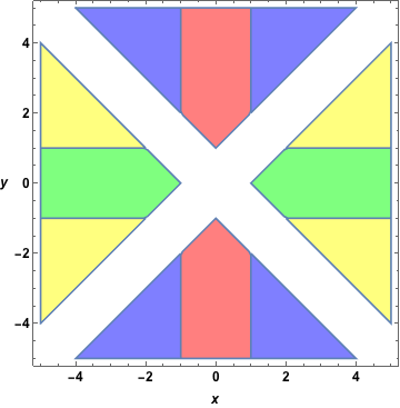
Figure 2: Left: Regions of convergence of the analytic continuations of the Appell $F_{2}$ series given in Eqs.(10) (in red) and (10) (in blue) and of the symmetrical relations obtained from them (in green and yellow respectively). Right: Same figure when one adds the ROC of Fig. 1 (Left) and when one applies the Euler transforms of $F_{2}$ given in Eq. (6) on all these results.

As mentioned above, two symmetrical relations can be computed from the Mellin-Barnes representation, which can also be obtained using the symmetry property of Eq.(5) applied to Eq.(10) and Eq.(11). These symmetrical analytic continuations converge in the green and yellow regions of Fig. 2 (Left).

With no further transformation of the MB integral one cannot obtain, from the latter, other series representations than those presented above. However, using the three Euler transformations shown in Eq.(6), it is possible to derive 12 other formulas, that we do not list here and which, alltogether, allow us to obtain the total convergence region of Fig. 2 (Right).

When added to the usual $F_{2}$ series definition and its three Euler transformations, these 16 linear transformations show that a good part of the $(x,y)$ real plane can be reached, but one can see on the plot that several regions are still missing. This is the aim of the rest of this paper to fill this gap, following an alternative method of analytic continuation.

4 Analytic continuation from Olsson’s method

In [16], Olsson obtained the complete set of solutions of the Appell $F_{1}$ system of partial differential equations, as well as the relations that connect them, thereby obtaining analytic continuation formulas of $F_{1}$ in the neighbourhood of any of its singularities. His method rests on the application of various transformations and analytic continuations of the ${}_{2}F_{1}$ Gauss hypergeometric series on the Appell $F_{1}$ written as an infinite sum of ${}_{2}F_{1}$. We follow this procedure below to derive analytic continuation formulas for $F_{2}$.

One will note that, except for the results of Section 3, which are briefly rederived following Olsson’s method in the beginning of subsection 4.2, the regions of convergence of all the analytic continuation formulas presented in Section 4 are trivial. They can be straightforwardly obtained as the intersections of the regions defined by the modulus, smaller than unity, of each of the arguments of the series involved in these formulas. This is due to the simple form of these series, as it is explictly shown in one example in Section 4.1.1.

4.1 Analytic continuation around (0,1)

We begin our study by the derivation of analytic continuations of the Appell $F_{2}$ series around the point $(0,1)$. Note that, still by the symmetry shown in Eq. (5), the final expressions can be used to obtain analytic continuations around the point $(1,0)$. Several different formulas will be necessary to cover the whole neighbourhood of these points.

4.1.1 A first analytic continuation

Rewriting $F_{2}$ as an infinite sum of ${}_{2}F_{1}$, one gets

$$F_{2}(a,b_{1},b_{2};c_{1},c_{2};x,y)=\sum_{m=0}^{\infty}\frac{(a)_{m}(b_{1})_{m}}{(c_{1})_{m}m!}x^{m}\,_{2}F_{1}(a+m,b_{2};c_{2};y)$$ (18)

where one can now use the well-known analytic continuation of ${}_{2}F_{1}(a,b,c;z)$ around $z=1$ given by

$${}_{2}F_{1}(a,b,c;z) =\frac{\Gamma(c)\Gamma(c-a-b)}{\Gamma(c-a)\Gamma(c-b)}\,_{2}F_{1}(a,b,a+b-c+1;1-z)$$

$$+\frac{\Gamma(c)\Gamma(a+b-c)}{\Gamma(a)\Gamma(b)}(1-z)^{c-a-b}\,_{2}F_{1}(c-a,c-b,c-a-b+1;1-z)$$ (19)

Substituting and simplifying, one obtains

$$F_{2}(a,b_{1},b_{2};c_{1},c_{2};x,y)=\frac{\Gamma(c_{2})\Gamma(c_{2}-b_{2}-a)}{\Gamma(c_{2}-a)\Gamma(c_{2}-b_{2})}F{}^{1:2;1}_{1:1;0}\left[\begin{array}[]{c@{{}:{}}c@{;{}}c}a&b_{1},1+a-c_{2}&b_{2}\\[4.30554pt] a+b_{2}-c_{2}+1&c_{1}&{-}\mkern-7.0mu\cleaders\hbox{$\mkern-2.0mu-\mkern-2.0mu$}\hfill\mkern-7.0mu{-}\end{array}\;\middle|\;x,1-y\right]$$ (22)

$$+\frac{\Gamma(c_{2})\Gamma(a+b_{2}-c_{2})}{\Gamma(a)\Gamma(b_{2})}(1-y)^{c_{2}-b_{2}-a}\,\tilde{F}{}^{1:1;2}_{1:0;1}\left[\begin{array}[]{c@{{}:{}}c@{;{}}c}c_{2}-a&c_{2}-b_{2}&b_{1},1+a-c_{2}\\[4.30554pt] 1+c_{2}-b_{2}-a&{-}\mkern-7.0mu\cleaders\hbox{$\mkern-2.0mu-\mkern-2.0mu$}\hfill\mkern-7.0mu{-}&c_{1}\end{array}\;\middle|\;1-y,\frac{x}{1-y}\right]$$ (25)

where we have used, for the Kampé de Fériet and $\tilde{F}$ series, the notation presented in the previous section.

As mentioned above, a simple look at the particular form of these series allows to straightforwardly conclude that the $F^{1:2;1}_{1:1;0}$ series converges for $|x|<1\wedge|1-y|<1$ (see Fig. 3 Left) and the $\tilde{F}{}^{1:1;2}_{1:0;1}$ series converges for $|\frac{x}{1-y}|<1\wedge|1-y|<1$ (see Fig. 3 Right). This is due to the fact that the convergence region of a hypergeometric series is independent of its parameters (exceptional values of the latter being excluded) which implies, in particular, that the cancellation of opposite elements in the characteristic list of this series does not affect its region of convergence [4]. In our present case of study, since the characteristic lists of the Kampé de Fériet and $\tilde{F}{}^{1:1;2}_{1:0;1}$ series are respectively $\{m+n,m,m,n,-(m+n),-m\}$ and $\{m-n,m,n,-(m-n),-n\}$, the cancellation property leads to a factorisation of these double series into single series whose convergence regions are trivial.

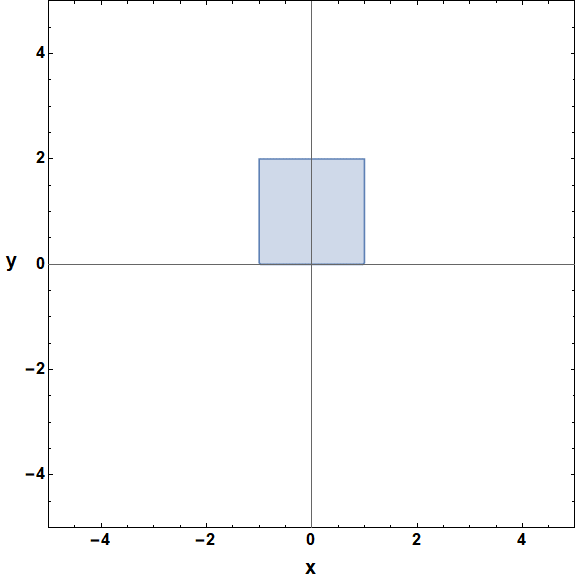
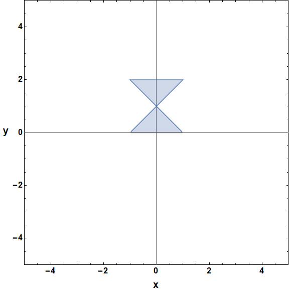
Figure 3: Left: ROC of $F^{1:2;1}_{1:1;0}$ in Eq.(25). Right: ROC of $\tilde{F}$ in Eq.(25).

Therefore, from Fig.3 one concludes that, for real values of $x$ and $y$, the ROC of the RHS of Eq. (25) is restricted to the region shown in Fig. 3 Right.
Using Eq.(5) we get the analytic continuation around (1,0) as

$$F_{2}(a,b_{1},b_{2};c_{1},c_{2};x,y)=\frac{\Gamma(c_{1})\Gamma(c_{1}-b_{1}-a)}{\Gamma(c_{1}-a)\Gamma(c_{1}-b_{1})}F{}^{1:2;1}_{1:1;0}\left[\begin{array}[]{c@{{}:{}}c@{;{}}c}a&b_{2},1+a-c_{1}&b_{1}\\[4.30554pt] a+b_{1}-c_{1}+1&c_{2}&{-}\mkern-7.0mu\cleaders\hbox{$\mkern-2.0mu-\mkern-2.0mu$}\hfill\mkern-7.0mu{-}\end{array}\;\middle|\;y,1-x\right]\\ \\ +\frac{\Gamma(c_{1})\Gamma(a+b_{1}-c_{1})}{\Gamma(a)\Gamma(b_{1})}(1-x)^{c_{1}-b_{1}-a}\tilde{F}{}^{1:1;2}_{1:0;1}\left[\begin{array}[]{c@{{}:{}}c@{;{}}c}c_{1}-a&c_{1}-b_{1}&b_{2},1+a-c_{1}\\[4.30554pt] 1+c_{1}-b_{1}-a&{-}\mkern-7.0mu\cleaders\hbox{$\mkern-2.0mu-\mkern-2.0mu$}\hfill\mkern-7.0mu{-}&c_{2}\end{array}\;\middle|\;1-x,\frac{y}{1-x}\right]$$ (26)

which now converges, still for real values of $x$ and $y$, in the region shown in Fig.4. One will note here that the regions shown in Fig.3 Right and Fig.4 are already covered by the formulas presented in Section 3.

Figure 4: ROC of the RHS of Eq.(26).

Looking at the ROC plots it is clear that the $\tilde{F}$ series prevents the analytic continuation in Eq.(25) (respectively Eq.(26)) to converge around the whole neighbourhood of $(0,1)$ (respectively $(1,0)$). More precisely, the constraint $|\frac{x}{1-y}|<1$ (respectively $|\frac{y}{1-x}|<1$) is responsible for that, which means that by going on with the analytic continuation process on its associated sum, one can probably derive another more interesting formula. This will be done in the next section where the obtained formula, in addition to reach the missing region around (0,1), will also be the starting point of another analytic continuation which is presented in Section 4.3.

4.1.2 A second analytic continuation

Since we have

$$\tilde{F}{}^{1:1;2}_{1:0;1}\left[\begin{array}[]{c@{{}:{}}c@{;{}}c}c_{2}-a&c_{2}-b_{2}&b_{1},1+a-c_{2}\\[4.30554pt] 1+c_{2}-b_{2}-a&{-}\mkern-7.0mu\cleaders\hbox{$\mkern-2.0mu-\mkern-2.0mu$}\hfill\mkern-7.0mu{-}&c_{1}\end{array}\;\middle|\;1-y,\frac{x}{1-y}\right]=\\ \sum_{m=0}^{\infty}\sum_{n=0}^{\infty}\frac{(c_{2}-a)_{m-n}(b_{1})_{n}(1+a-c_{2})_{n}(c_{2}-b_{2})_{m}}{(1+c_{2}-b_{2}-a)_{m-n}(c_{1})_{n}m!n!}(1-y)^{m}\Big{(}\frac{x}{1-y}\Big{)}^{n}$$ (27)

which can be rewritten as

$$\tilde{F}{}^{1:1;2}_{1:0;1}\left[\begin{array}[]{c@{{}:{}}c@{;{}}c}c_{2}-a&c_{2}-b_{2}&b_{1},1+a-c_{2}\\[4.30554pt] 1+c_{2}-b_{2}-a&{-}\mkern-7.0mu\cleaders\hbox{$\mkern-2.0mu-\mkern-2.0mu$}\hfill\mkern-7.0mu{-}&c_{1}\end{array}\;\middle|\;1-y,\frac{x}{1-y}\right]=\\ \sum_{m=0}^{\infty}\frac{(c_{2}-a)_{m}(c_{2}-b_{2})_{m}}{(1+c_{2}-b_{2}-a)_{m}m!}(1-y)^{m}\,_{3}F_{2}\left(\begin{matrix}a+b_{2}-c_{2}-m,&b_{1},&1+a-c_{2}\\ \\ &1+a-c_{2}-m,&c_{1}\end{matrix}\Bigg{|}{\frac{x}{1-y}}\right)$$ (28)

one can use the standard analytic continuation formula of ${}_{3}F_{2}$

$${}_{3}F_{2}\left(\begin{matrix}a_{1},&a_{2},&a_{3}\\ \\ &b_{1},&b_{2}\end{matrix}\Bigg{|}{z}\right) =\frac{\Gamma(b_{1})\Gamma(b_{2})\Gamma(a_{2}-a_{1})\Gamma(a_{3}-a_{1})}{\Gamma(a_{2})\Gamma(a_{3})\Gamma(b_{1}-a_{1})\Gamma(b_{2}-a_{1})}(-z)^{-a_{1}}\,_{3}F_{2}\left(\begin{matrix}a_{1},&1+a_{1}-b_{1},&1+a_{1}-b_{2}\\ \\ &1+a_{1}-a_{2},&1+a_{1}-a_{3}\end{matrix}\Bigg{|}{\frac{1}{z}}\right)$$ (29)

$$+\frac{\Gamma(b_{1})\Gamma(b_{2})\Gamma(a_{1}-a_{2})\Gamma(a_{3}-a_{2})}{\Gamma(a_{1})\Gamma(a_{3})\Gamma(b_{1}-a_{2})\Gamma(b_{2}-a_{2})}(-z)^{-a_{2}}\,_{3}F_{2}\left(\begin{matrix}a_{2},&1+a_{2}-b_{1},&1+a_{2}-b_{2}\\ \\ &1+a_{2}-a_{1},&1+a_{2}-a_{3}\end{matrix}\Bigg{|}{\frac{1}{z}}\right)$$

$$+\frac{\Gamma(b_{1})\Gamma(b_{2})\Gamma(a_{1}-a_{3})\Gamma(a_{2}-a_{3})}{\Gamma(a_{1})\Gamma(a_{2})\Gamma(b_{1}-a_{3})\Gamma(b_{2}-a_{3})}(-z)^{-a_{3}}\,_{3}F_{2}\left(\begin{matrix}a_{3},&1+a_{3}-b_{1},&1+a_{3}-b_{2}\\ \\ &1+a_{3}-a_{1},&1+a_{3}-a_{2}\end{matrix}\Bigg{|}{\frac{1}{z}}\right)$$

which allows to derive

$$\tilde{F}{}^{1:1;2}_{1:0;1}\left[\begin{array}[]{c@{{}:{}}c@{;{}}c}c_{2}-a&c_{2}-b_{2}&b_{1},1+a-c_{2}\\[4.30554pt] 1+c_{2}-b_{2}-a&{-}\mkern-7.0mu\cleaders\hbox{$\mkern-2.0mu-\mkern-2.0mu$}\hfill\mkern-7.0mu{-}&c_{1}\end{array}\;\middle|\;1-y,\frac{x}{1-y}\right]=$$ (32)

$$\left(\frac{x}{y-1}\right)^{-a-b_{2}+c_{2}}\frac{\Gamma\left(c_{1}\right)\Gamma\left(-a+b_{1}-b_{2}+c_{2}\right)}{\Gamma\left(b_{1}\right)\Gamma\left(-a-b_{2}+c_{1}+c_{2}\right)}\tilde{F}{}^{2:1;1}_{2:0;0}\left[\begin{array}[]{c@{{}:{}}c@{;{}}c}1-b_{2},-a+b_{1}-b_{2}+c_{2}&c_{2}-b_{2}&b_{2}\\[4.30554pt] -a-b_{2}+c_{2}+1,-a-b_{2}+c_{1}+c_{2}&{-}\mkern-7.0mu\cleaders\hbox{$\mkern-2.0mu-\mkern-2.0mu$}\hfill\mkern-7.0mu{-}&{-}\mkern-7.0mu\cleaders\hbox{$\mkern-2.0mu-\mkern-2.0mu$}\hfill\mkern-7.0mu{-}\end{array}\;\middle|\;x,\frac{1-y}{x}\right]$$ (35)

$$+\left(\frac{x}{y-1}\right)^{-b_{1}}\frac{\Gamma\left(c_{1}\right)\Gamma\left(a-b_{1}+b_{2}-c_{2}\right)}{\Gamma\left(c_{1}-b_{1}\right)\Gamma\left(a+b_{2}-c_{2}\right)}F{}^{1:1;2}_{1:0;1}\left[\begin{array}[]{c@{{}:{}}c@{;{}}c}-a+b_{1}+c_{2}&c_{2}-b_{2}&b_{1}-c_{1}+1,b_{1}\\[4.30554pt] -a+b_{1}-b_{2}+c_{2}+1&{-}\mkern-7.0mu\cleaders\hbox{$\mkern-2.0mu-\mkern-2.0mu$}\hfill\mkern-7.0mu{-}&-a+b_{1}+c_{2}\end{array}\;\middle|\;1-y,\frac{1-y}{x}\right]$$ (38)

Substituting this result back in Eq.(25) one gets

$$F_{2}(a,b_{1},b_{2};c_{1},c_{2};x,y)= \frac{\Gamma(c_{2})\Gamma(-a-b_{2}+c_{2})}{\Gamma(c_{2}-a)\Gamma(c_{2}-b_{2})}{F}{}^{1:2;1}_{1:1;0}\left[\begin{array}[]{c@{{}:{}}c@{;{}}c}a&a-c_{2}+1,b_{1}&b_{2}\\[4.30554pt] a+b_{2}-c_{2}+1&c_{1}&-\end{array}\;\middle|\;x,1-y\right]$$ (41)

$$+(1-y)^{-a-b_{2}+c_{2}}\left(\frac{x}{y-1}\right)^{-a-b_{2}+c_{2}}\frac{\Gamma(c_{1})\Gamma(c_{2})\Gamma(a+b_{2}-c_{2})\Gamma(-a+b_{1}-b_{2}+c_{2})}{\Gamma(a)\Gamma(b_{1})\Gamma(b_{2})\Gamma(-a-b_{2}+c_{1}+c_{2})}$$

$$\times\tilde{F}{}^{2:1;1}_{2:0;0}\left[\begin{array}[]{c@{{}:{}}c@{;{}}c}a+b_{2}-c_{2},a+b_{2}-c_{2}-c_{1}+1&b_{2}&c_{2}-b_{2}\\[4.30554pt] b_{2},a-b_{1}+b_{2}-c_{2}+1&-&-\end{array}\;\middle|\;\frac{1-y}{x},x\right]$$ (44)

$$+\left(\frac{x}{y-1}\right)^{-b_{1}}(1-y)^{-a-b_{2}+c_{2}}\frac{\Gamma(c_{1})\Gamma(c_{2})\Gamma(a-b_{1}+b_{2}-c_{2})}{\Gamma(a)\Gamma(b_{2})\Gamma(c_{1}-b_{1})}$$

$$\times{F}{}^{1:2;1}_{1:1;0}\left[\begin{array}[]{c@{{}:{}}c@{;{}}c}-a+b_{1}+c_{2}&b_{1},b_{1}-c_{1}+1&c_{2}-b_{2}\\[4.30554pt] -a+b_{1}-b_{2}+c_{2}+1&-a+b_{1}+c_{2}&-\end{array}\;\middle|\;\frac{1-y}{x},1-y\right]$$ (47)

which, trivially, converges in $|\frac{1-y}{x}|<1\wedge|x|<1\wedge|1-y|<1$ (see, for real values of $x$ and $y$, Fig. 5 Left).

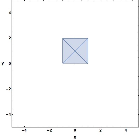
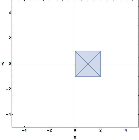
Figure 5: Left: ROC of the RHS of Eq.(41), Middle: Reached region around $(0,1)$, Right: Corresponding reached region around $(1,0)$.

Therefore, taking into account the results of Section 4.1.1, we are now able to reach the whole neighborhood of $(0,1)$ (see Fig.5 Middle) with the exception of the boundaries of the ROCs which will be considered later.

As before we can now straightforwardly get the corresponding continuation around $(1,0)$ using Eq.(5). Together with the previous symmetrical analytic continuation given in Eq.(26) we can then reach the whole neighborhood of $(1,0)$, except on the boundaries of the ROCs (see Fig.5 Right).

4.2 Analytic continuation around $(0,\infty)$ and $(\infty,\infty)$

Next we turn to the analytic continuation around the singular point $(0,\infty)$. This analytic continuation will then be used to find the analytic continuation around the singular point $(\infty,\infty)$. Moreover, as before, symmetry will give us the $(\infty,0)$ case. The corresponding formulas and their convergence regions have already been derived in Section 3, from the Mellin-Barnes representation of $F_{2}$, but for completeness we briefly show here how they can also be obtained from Olsson’s method (see also Chapter 9 of [4]).

To find the continuation around $(0,\infty)$ we start again with Eq.(18) and use the standard analytic continuation formula for ${}_{2}F_{1}$ given by

$${}_{2}F_{1}(a,b,c;z) =\frac{\Gamma(c)\Gamma(b-a)}{\Gamma(b)\Gamma(c-a)}(-z)^{-a}\,_{2}F_{1}\left(a,a-c+1,a-b+1;\frac{1}{z}\right)$$

$$+\frac{\Gamma(c)\Gamma(a-b)}{\Gamma(a)\Gamma(c-b)}(-z)^{-b}\,_{2}F_{1}\left(b,b-c+1,b-a+1;\frac{1}{z}\right)$$ (48)

This directly gives Eq.(10).

Then, in order to find the analytic continuation around $(\infty,\infty)$, we observe that we just need to continue the Horn $H_{2}$ series in Eq.(10), as the other series already converges around $(\infty,\infty)$. So, writing

$$H_{2}\Big{(}a-b_{2},b_{1},b_{2},b_{2}-c_{2}+1;c_{1};x,-\frac{1}{y}\Big{)}=\sum_{n=0}^{\infty}\frac{(a-b_{2})_{-n}(b_{2})_{n}(b_{2}-c_{2}+1)_{n}}{n!}\Big{(}-\frac{1}{y}\Big{)}^{n}\,_{2}F_{1}(a-b_{2}-n,b_{1},c_{1};x)$$ (49)

and using once more Eq.(48) we get

$$H_{2}\Big{(}a-b_{2},b_{1},b_{2},b_{2}-c_{2}+1;c_{1};x,-\frac{1}{y}\Big{)}=\\ \frac{\Gamma(c_{1})\Gamma(b_{1}+b_{2}-a)}{\Gamma(b_{1})\Gamma(c_{1}+b_{2}-a)}(-x)^{b_{2}-a}\tilde{F}{}^{2:0;2}_{1:0;0}\left[\begin{array}[]{c@{{}:{}}c@{;{}}c}a-b_{2},a-b_{2}-c_{1}+1&{-}\mkern-7.0mu\cleaders\hbox{$\mkern-2.0mu-\mkern-2.0mu$}\hfill\mkern-7.0mu{-}&b_{2},b_{2}-c_{2}+1\\[4.30554pt] a-b_{2}-b_{1}+1&{-}\mkern-7.0mu\cleaders\hbox{$\mkern-2.0mu-\mkern-2.0mu$}\hfill\mkern-7.0mu{-}&{-}\mkern-7.0mu\cleaders\hbox{$\mkern-2.0mu-\mkern-2.0mu$}\hfill\mkern-7.0mu{-}\end{array}\;\middle|\;\frac{1}{x},\frac{x}{y}\right]\\ \\ +\frac{\Gamma(c_{1})\Gamma(a-b_{1}-b_{2})}{\Gamma(a-b_{2})\Gamma(c_{1}-b_{1})}(-x)^{-b_{1}}F_{3}\Big{(}b_{1},b_{2},b_{1}-c_{1}+1,b_{2}-c_{2}+1,b_{1}+b_{2}-a+1;\frac{1}{x},\frac{1}{y}\Big{)}$$ (50)

Substituting the above back in Eq.(10) we get Eq.(11).

The regions of convergence of Eqs.(10) and (11) are ploted in Fig. 2 Left.

4.3 Analytic Continuation around $(\infty,1)$

Looking at the ROC of the second continuation around (0,1), Eq.(41), we note that $F{}^{1:2;1}_{1:1;0}(...;\frac{1-y}{x},1-y)$ converges in the entire neighborhood of $(\infty,1)$. Therefore, in order to derive an analytic continuation valid in this region, we only need to analytically continue the remaining two series of Eq.(41). Let us consider the first series which reads

$$F{}^{1:2;1}_{1:1;0}\left[\begin{array}[]{c@{{}:{}}c@{;{}}c}a&b_{1},1+a-c_{2}&b_{2}\\[4.30554pt] a+b_{2}-c_{2}+1&c_{1}&{-}\mkern-7.0mu\cleaders\hbox{$\mkern-2.0mu-\mkern-2.0mu$}\hfill\mkern-7.0mu{-}\end{array}\;\middle|\;x,1-y\right]=\\ \\ \sum_{n=0}^{\infty}\frac{(a)_{n}(b_{2})_{n}}{(a+b_{2}-c_{2}+1)_{n}n!}(1-y)^{n}\,_{3}F_{2}\left(\begin{matrix}a+n,&b_{1},&1+a-c_{2}\\ \\ &a+b_{2}-c_{2}+1+n,&c_{1}\end{matrix}\Bigg{|}{x}\right)$$ (51)

Applying Eq.(29) and simplifying we get

$$F{}^{1:2;1}_{1:1;0}\left[\begin{array}[]{c@{{}:{}}c@{;{}}c}a&b_{1},1+a-c_{2}&b_{2}\\[4.30554pt] a+b_{2}-c_{2}+1&c_{1}&{-}\mkern-7.0mu\cleaders\hbox{$\mkern-2.0mu-\mkern-2.0mu$}\hfill\mkern-7.0mu{-}\end{array}\;\middle|\;x,1-y\right]=$$ (54)

$$\frac{\Gamma(1+a-c_{2}-b_{1})\Gamma(c_{1})\Gamma(a-b_{1})\Gamma(a+b_{2}-c_{2}+1)}{\Gamma(1+a-c_{2})\Gamma(c_{1}-b_{1})\Gamma(a)\Gamma(a+b_{2}-b_{1}-c_{2}+1)}(-x)^{b_{1}}\tilde{F}{}^{1:2;1}_{1:1;0}\left[\begin{array}[]{c@{{}:{}}c@{;{}}c}b_{1}+c_{2}-a-b_{2}&1+b_{1}-c_{1},b_{1}&b_{2}\\[4.30554pt] 1-a+b_{1}&b_{1}+c_{2}-a&{-}\mkern-7.0mu\cleaders\hbox{$\mkern-2.0mu-\mkern-2.0mu$}\hfill\mkern-7.0mu{-}\end{array}\;\middle|\;\frac{1}{x},1-y\right]$$ (57)

$$+\frac{\Gamma(b_{1}+c_{2}-a-1)\Gamma(c_{1})\Gamma(c_{2}-1)\Gamma(a+b_{2}-c_{2}+1)}{\Gamma(b_{1})\Gamma(c_{1}+c_{2}-a-1)\Gamma(a)\Gamma(b_{2})}(-x)^{c_{2}-a-1}$$

$$\hskip 85.35826pt\times\tilde{F}{}^{1:2;1}_{1:1;0}\left[\begin{array}[]{c@{{}:{}}c@{;{}}c}1-b_{2}&2+a-c_{2}-c_{1},1+a-c_{2}&b_{2}\\[4.30554pt] 2-c_{2}&a-c_{2}-b_{1}+2&{-}\mkern-7.0mu\cleaders\hbox{$\mkern-2.0mu-\mkern-2.0mu$}\hfill\mkern-7.0mu{-}\end{array}\;\middle|\;\frac{1}{x},1-y\right]$$ (60)

$$+\frac{\Gamma(c_{1})\Gamma(b_{1}-a)\Gamma(1-c_{2})\Gamma(1+a+b_{2}-c_{2})}{\Gamma(b_{1})\Gamma(1+a-c_{2})\Gamma(1+b_{2}-c_{2})\Gamma(c_{1}-a)}(-x)^{-a}F{}^{2:1;1}_{2:0;0}\left[\begin{array}[]{c@{{}:{}}c@{;{}}c}a,1+a-c_{1}&c_{2}-b_{2}&b_{2}\\[4.30554pt] c_{2},1+a-b_{1}&{-}\mkern-7.0mu\cleaders\hbox{$\mkern-2.0mu-\mkern-2.0mu$}\hfill\mkern-7.0mu{-}&{-}\mkern-7.0mu\cleaders\hbox{$\mkern-2.0mu-\mkern-2.0mu$}\hfill\mkern-7.0mu{-}\end{array}\;\middle|\;\frac{1}{x},\frac{1-y}{x}\right]$$ (63)

This is sufficient for this series. Now, taking the third series in Eq.(41), which can also be written as an infinite sum of ${}_{3}F_{2}$ hypergeometric functions:

$$\tilde{F}{}^{2:1;0}_{2:0;0}\left[\begin{array}[]{c@{{}:{}}c@{;{}}c}a+b_{2}-c_{2},1+b_{2}+a-c_{1}-c_{2}&b_{2},c_{2}-b_{2}&{-}\mkern-7.0mu\cleaders\hbox{$\mkern-2.0mu-\mkern-2.0mu$}\hfill\mkern-7.0mu{-}\\[4.30554pt] 1+a+b_{2}-b_{1}-c_{2},b_{2}&{-}\mkern-7.0mu\cleaders\hbox{$\mkern-2.0mu-\mkern-2.0mu$}\hfill\mkern-7.0mu{-}&{-}\mkern-7.0mu\cleaders\hbox{$\mkern-2.0mu-\mkern-2.0mu$}\hfill\mkern-7.0mu{-}\end{array}\;\middle|\;\frac{1-y}{x},x\right]=\\ \\ \sum_{m=0}^{\infty}\frac{(a+b_{2}-c_{2})_{m}(1+b_{2}+a-c_{2}-c_{1})_{m}}{(1+a+b_{2}-b_{1}-c_{2})_{m}m!}\left(\frac{1-y}{x}\right)^{m}\\ \times\,_{3}F_{2}\left(\begin{matrix}c_{2}-b_{2},&1-b_{2}-m,&c_{2}+b_{1}-b_{2}-a-m\\ \\ &1+c_{2}-b_{2}-a-m,&c_{1}+c_{2}-a-b_{2}-m\end{matrix}\Bigg{|}{x}\right)$$ (64)

one has, using Eq.(29) once more,

$$\tilde{F}{}^{2:1;0}_{2:0;0} \left[\begin{array}[]{c@{{}:{}}c@{;{}}c}a+b_{2}-c_{2},1+b_{2}+a-c_{1}-c_{2}&b_{2},c_{2}-b_{2}&{-}\mkern-7.0mu\cleaders\hbox{$\mkern-2.0mu-\mkern-2.0mu$}\hfill\mkern-7.0mu{-}\\[4.30554pt] 1+a+b_{2}-b_{1}-c_{2},b_{2}&{-}\mkern-7.0mu\cleaders\hbox{$\mkern-2.0mu-\mkern-2.0mu$}\hfill\mkern-7.0mu{-}&{-}\mkern-7.0mu\cleaders\hbox{$\mkern-2.0mu-\mkern-2.0mu$}\hfill\mkern-7.0mu{-}\end{array}\;\middle|\;\frac{1-y}{x},x\right]=$$ (67)

$$(-x)^{b_{2}-c_{2}}\frac{\Gamma\left(1-c_{2}\right)\Gamma\left(b_{1}-a\right)\Gamma\left(-a-b_{2}+c_{2}+1\right)\Gamma\left(-a-b_{2}+c_{1}+c_{2}\right)}{\Gamma(1-a)\Gamma\left(1-b_{2}\right)\Gamma\left(c_{1}-a\right)\Gamma\left(-a+b_{1}-b_{2}+c_{2}\right)}$$

$$\times F{}^{2:1;1}_{2:0;0}\left[\begin{array}[]{c@{{}:{}}c@{;{}}c}a,a-c_{1}+1&c_{2}-b_{2}&b_{2}\\[4.30554pt] c_{2},a-b_{1}+1&{-}\mkern-7.0mu\cleaders\hbox{$\mkern-2.0mu-\mkern-2.0mu$}\hfill\mkern-7.0mu{-}&{-}\mkern-7.0mu\cleaders\hbox{$\mkern-2.0mu-\mkern-2.0mu$}\hfill\mkern-7.0mu{-}\end{array}\;\middle|\;\frac{1}{x},\frac{1-y}{x}\right]$$ (70)

$$+\frac{\Gamma(b_{1}+c_{2}-a-1)\Gamma(1+c_{2}-b_{2}-a)\Gamma(c_{1}+c_{2}-a-b_{2})\Gamma(c_{2}-1)}{\Gamma(c_{2}-a)\Gamma(c_{2}-b_{2})\Gamma(c_{1}+c_{2}-a-1)\Gamma(b_{1}+c_{2}-a-b_{2})}(-x)^{-1+b_{2}}$$

$$\times\tilde{F}{}^{1:2;1}_{1:1;0}\left[\begin{array}[]{c@{{}:{}}c@{;{}}c}1-b_{2}&2+a-c_{2}-c_{1},1+a-c_{2}&b_{2}\\[4.30554pt] 2-c_{2}&a-c_{2}-b_{1}+2&{-}\mkern-7.0mu\cleaders\hbox{$\mkern-2.0mu-\mkern-2.0mu$}\hfill\mkern-7.0mu{-}\end{array}\;\middle|\;\frac{1}{x},1-y\right]$$ (73)

$$+(-x)^{a-b_{1}+b_{2}-c_{2}}\frac{\Gamma\left(a-b_{1}\right)\Gamma\left(a-b_{1}-c_{2}+1\right)\Gamma\left(-a-b_{2}+c_{2}+1\right)\Gamma\left(-a-b_{2}+c_{1}+c_{2}\right)}{\Gamma\left(1-b_{1}\right)\Gamma\left(1-b_{2}\right)\Gamma\left(c_{1}-b_{1}\right)\Gamma\left(c_{2}-b_{2}\right)}$$

$$\times\tilde{F}{}^{1:2;1}_{1:1;0}\left[\begin{array}[]{c@{{}:{}}c@{;{}}c}-a+b_{1}-b_{2}+c_{2}&b_{1},b_{1}-c_{1}+1&b_{2}\\[4.30554pt] -a+b_{1}+1&-a+b_{1}+c_{2}&{-}\mkern-7.0mu\cleaders\hbox{$\mkern-2.0mu-\mkern-2.0mu$}\hfill\mkern-7.0mu{-}\end{array}\;\middle|\;\frac{1}{x},1-y\right]$$ (76)

Substituting the above two results in Eq.(41) and simplifying we get

$$F_{2}(a,b_{1},b_{2};c_{1},c_{2};x,y)=$$

$$\frac{\Gamma(c_{1})\Gamma(c_{2})\Gamma(a-b_{1})\Gamma(-a+b_{1}-b_{2}+c_{2})}{\Gamma(a)\Gamma(c_{1}-b_{1})\Gamma(c_{2}-b_{2})\Gamma(-a+b_{1}+c_{2})}\left(-x\right)^{-b_{1}}$$

$$\times\tilde{F}{}^{1:2;1}_{1:1;0}\left[\begin{array}[]{c@{{}:{}}c@{;{}}c}b_{1}+c_{2}-a-b_{2}&1+b_{1}-c_{1},b_{1}&b_{2}\\[4.30554pt] 1-a+b_{1}&b_{1}+c_{2}-a&{-}\mkern-7.0mu\cleaders\hbox{$\mkern-2.0mu-\mkern-2.0mu$}\hfill\mkern-7.0mu{-}\end{array}\;\middle|\;\frac{1}{x},1-y\right]$$ (79)

$$+\frac{\Gamma\left(c_{1}\right)\Gamma\left(b_{1}-a\right)}{\Gamma\left(b_{1}\right)\Gamma\left(c_{1}-a\right)}\left(-x\right)^{-a}F^{2:1;1}_{2:0;0}\left[\begin{array}[]{c@{{}:{}}c@{;{}}c}a,1+a-c_{1}&c_{2}-b_{2}&b_{2}\\[4.30554pt] c_{2},1+a-b_{1}&{-}\mkern-7.0mu\cleaders\hbox{$\mkern-2.0mu-\mkern-2.0mu$}\hfill\mkern-7.0mu{-}&{-}\mkern-7.0mu\cleaders\hbox{$\mkern-2.0mu-\mkern-2.0mu$}\hfill\mkern-7.0mu{-}\end{array}\;\middle|\;\frac{1}{x},\frac{1-y}{x}\right]$$ (82)

$$+\frac{\Gamma\left(c_{1}\right)\Gamma\left(c_{2}\right)\Gamma\left(a-b_{1}+b_{2}-c_{2}\right)}{\Gamma(a)\Gamma\left(b_{2}\right)\Gamma\left(c_{1}-b_{1}\right)}\left(-x\right)^{-b_{1}}(1-y)^{-a+b_{1}-b_{2}+c_{2}}$$

$$\times F{}^{1:2;1}_{1:1;0}\left[\begin{array}[]{c@{{}:{}}c@{;{}}c}c_{2}-a+b_{1}&b_{1},1+b_{1}-c_{1}&c_{2}-b_{2}\\[4.30554pt] 1+b_{1}+c_{2}-b_{2}-a&c_{2}-a+b_{1}&{-}\mkern-7.0mu\cleaders\hbox{$\mkern-2.0mu-\mkern-2.0mu$}\hfill\mkern-7.0mu{-}\end{array}\;\middle|\;\frac{1-y}{x},1-y\right]$$ (85)

where $\tilde{F}(...;\frac{1}{x},1-y)$ converges for $|\frac{1}{x}|<1\wedge|1-y|<1$ (see Fig.6 Left), $F^{2:1;1}_{2:0;0}(...;\frac{1}{x},\frac{1-y}{x})$ converges for $\Big{|}\frac{1}{x}\Big{|}<1\wedge|\frac{1-y}{x}|<1$ (see Fig.6 Middle) and $F^{1:2;1}_{1:1;0}(...;\frac{1-y}{x},1-y)$ converges for $|1-y|<1\wedge|\frac{1-y}{x}|<1$ (see Fig.6 Right).

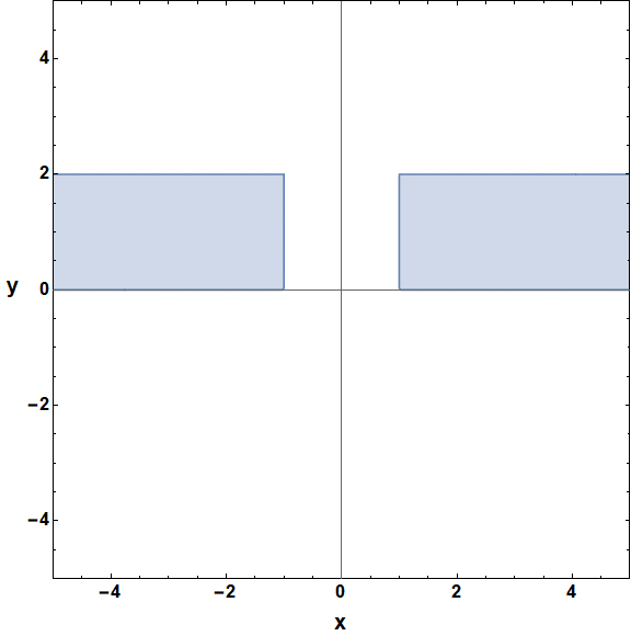
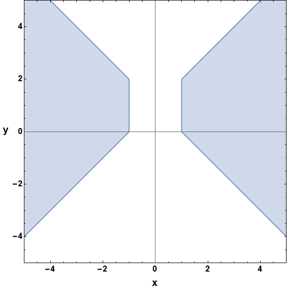
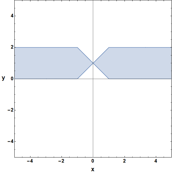
Figure 6: Left: ROC of $\tilde{F}(...;\frac{1}{x},1-y)$. Middle: ROC of $F^{2:1;1}_{2:0;0}(...;\frac{1}{x},\frac{1-y}{x})$. Right: ROC of $F^{1:2;1}_{1:1;0}(...;\frac{1-y}{x},1-y)$.

It is therefore clear that the analytic continuation in Eq.(85) converges in the region shown in Fig.6 (Left), for real values of $x$ and $y$.

Using Eq.(5) we get another analytic continuation around $(1,\infty)$ which converges in the region $|\frac{1}{y}|<1\wedge|1-x|<1\wedge|\frac{1-x}{y}|<1$, for real values of $x$ and $y$, see Fig.7 (Left).

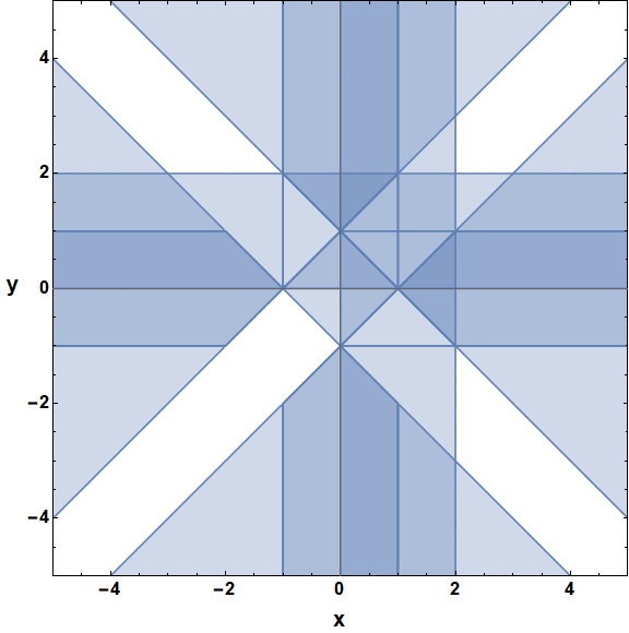
Figure 7: Left: See the text. Right: Regions covered using all the so far obtained analytic continuations.

4.4 Using Euler transformations

In the previous sections, we presented 10 different linear transformations of the Appell $F_{2}$ double hypergeometric series which analytically continue the latter in various regions of the $(x,y)$ space. Now, using these results, it is possible to derive many other analytic continuations. Indeed, if, instead of starting from the series definition of $F_{2}$, Eq.(1), one starts from the alternative series representation given by any of the three Euler transformations shown in Eq.(6), one can use the 10 formulas above to try 30 different ways to derive other analytic continuations. In the total of the various series representations that can be obtained by this exercise (which amounts to 44 if one includes the series definition of $F_{2}$ and its three Euler transformations), we noticed that 18 are sufficient to cover the whole $(x,y)$ space, except some particular points, namely $(1,0)$, $(0,1)$, $(1,1)$, $(-1,1)$, $(1,-1)$, and $(\frac{1}{2},\frac{1}{2})$. Adding the other analytic continuations does not help to reach the missing points. These 18 formulas are listed in the Appendix with plots of their convergence regions, and they form, with the remaining 26 series representations whose expressions are not given explicitly here to lighten the paper, the basis of the AppellF2 Mathematica package, presented in Section 5 and dedicated to the numerical evaluation of the Appell $F_{2}$ function.

5 The AppellF2 Mathematica package

Using the series representations of the Appell $F_{2}$ function derived above and listed in the Appendix, the package AppellF2 can find the numerical value of the Appell $F_{2}$ function, in nonlogarithmic situations (i.e. for generic values of the Pochhammer parameters), for arbitrary real values of $x$ and $y$ with the exception of the points that belong to the singular curves of Fig.1 Right for which the result cannot be obtained for all values of the Pochhammer parameters.

Let us demonstrate the working principle of the package AppellF2 below and apply it to some examples later in this section. AppellF2 can be used on Mathematica v11.3 and beyond.

5.1 Algorithm of AppellF2

The AppellF2 package works as follows:

1. Except if the given $(x,y)$ point of evaluation is any of the special points that belong to the singular curves of Fig.1 Right, which are “Pochhammer dependent”, all the series representations of $F_{2}$ that are valid at the given point are found by the package.

2. Although the same numerical result, for a given precision, will be obtained with any of these series if one sums enough terms, some series will converge faster than others (for instance if the point is not close to the boundary of their convergence region). Therefore, in order to improve the speed of the package, an experimental criterion has been implemented in the code in such a way that the “best” series representation, from the convergence point of view, is selected. The criterion is defined as follows.

   A typical series representation of $F_{2}$ consists of more than one series.

   $$F_{2}(a,b_{1},b_{2},c_{1},c_{2},x,y)=\sum_{i}U_{i}$$

   $$U_{i}=\sum_{m,n=0}^{\infty}V_{i}(a,b_{1},b_{2},c_{1},c_{2},x,y,m,n)$$

   For each $U_{i}$, the package calculates $r_{i}$ and $s_{i}$ as written below, for the given values of Pochhammer parameters and $x,y$ (for readibility we have suppressed the dependence of $V_{i}$ on the Pochhammer parameters and on $x$ and $y$):

   $$s_{i}=\left|\frac{V_{i}(m+1,n)}{V_{i}(m,n)}\right|_{m,n=100},\hskip 28.45274ptt_{i}=\left|\frac{V_{i}(m,n+1)}{V_{i}(m,n)}\right|_{m,n=100}$$

   The values of $m$ and $n$ have been experimentally chosen to be 100 here but some other values can be used.

   The rate of convergence for a series $U_{i}$ is chosen as $r_{i}=\sqrt{s_{i}^{2}+t_{i}^{2}}$. In general, all the series of a given series representation have different rates of convergence. We thus define the rate of convergence of that series representation to be the maximum of the rates of convergence of all of its involved series. Therefore, the rate of convergence of a series representation is

   $$R=\textrm{Max}\{r_{i}\}$$

   Thus, when comparing the various series representations that are valid at the same $(x,y)$ point, the one that has the smallest $R$ is selected.

3. The numerical evaluation is then performed using partial sums of the best series, for the chosen values of Pochhammer parameters and $x$ and $y$, upto a given number of terms. The output is returned at a given precision.

5.2 Demonstration

We now demonstrate the usage of the package AppellF2. After downloading the package in the same directory as the notebook, it is called as follows

     In[]:SetDirectory[NotebookDirectory[]];  In[]:=<<AppellF2.wl  AppellF2.wl v1.0  Authors : Souvik Bera & Tanay Pathak     

The command AppellF2, computing the numerical value of the $F_{2}$ function, can be called as,

     In[]:=AppellF2[a, b1, b2, c1, c2, x, y, p, terms, F2show->True]     Here, a,b1,b2,c1,c2 are the Pochhammer values given by the user, x,y is the point of evaluation, p is the required precision of the output (it gives the number of desired significant digits) and terms is the number of terms in the numerical summation for each summation index. F2show is an option with default value False. When it is made True, one can see the evaluation of the summation in real time.

As an example, the below command finds the value of $F_{2}$ upto $4$ significant digits at the point $(-2.311,5.322)$ with Pochhammer values $a=2.2345,b_{1}=3.363,b_{2}=0.242,c_{1}=8.3452$ and $c_{2}=0.657$ by evaluating the summation upto $100$ terms for both the summation indices.

     In[]:=AppellF2[2.2345, 3.363, 0.242, 8.3452, 0.657,-2.311, 5.322, 4, 100, F2show->False]     For this call, the package gives

     valid series:{{10},{15},{18},{26},{29},{43}}  convergence rates:{{0.59,10},{0.66,26},{0.68,18},{0.94,29},{0.95,43},{1.09,15}}  selected series: 10    Out[]=0.09334 - 0.06847 I     One can see that there are 6 series representations valid at the point $(-2.311,5.322)$ and that series $\#10$ is the best converging series that is chosen for the evaluation.

One will note that the specific command F2findall can be directly called to find which series are valid at a given point. For the example above,

     In[]:=F2findall[{-2.311, 5.322}]    Out[]={10, 15, 18, 26, 29, 43}     

In order to see the expression of any of the 44 series representations used in the package, and its region of convergence, the command F2expose can be used.

     In[]:=F2expose[15]    Out[]= {Abs[(-1 + x + y)/x]< 1&&Abs[x/(-1 + x)]<1,(1/(m! n!))((1-x)^{-a}) Gamma[c2]...}     The output above, which, due to its length, has been partly suppressed here, is a list containing the ROC of the series representation followed by the expression of the corresponding series (here $\#15$ which, from the correspondence Table 3 of the appendix, is $S_{7}$, see Eq.(124)).

The command F2ROC gives the plot of the ROC of the series representation #, along with the point (x,y), for a given range.

     F2ROC[{x,y}, #, range]     For instance, the call F2ROC[{-2.311, 5.322}, 15, {-6, 6}] gives the output shown in Fig. 8.

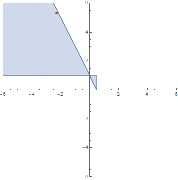
Figure 8: Output of F2ROC[{-2.311, 5.322}, 15, {-6, 6}]. The red dot is $(x,y)$=$(-2.311,5.322)$.

Finally, the user can chose which series representation he wants for the evaluation at a given point, using the command F2evaluate. For example,

     In[]:=F2evaluate[10, {2.2345, 3.363, 0.242, 8.3452, 0.657, -2.311, 5.322}, 10, 100]    Out[]=0.09333639793 - 0.06847416686 I     gives the values of $F_{2}(2.2345,3.363,0.242;8.3452,0.657;-2.311,5.322)$ derived from the series representation $\#10$ at 10 precision with 100 terms for each summation index.

5.3 Numerical tests

We have tested the AppellF2 package by computing 200 randomly generated points: 100 points with the ranges of random values of the Pochhammer parameters $a,b_{1},b_{2},c_{1}$ and $c_{2}$ and of the $x$ and $y$ variables being $[-7,7]$, and 100 points with random complex values of the Pochhammer parameters (with real and imaginary parts in the range $[-7,7]$).

For each of these 200 points, the series representations that are valid there all match numerically. As some of the series converge faster than others at a given point, it is sometimes necessary to increase the number of terms in the partial sums for those series that converge slowly.

We have also compared these results to the Maple inbuilt AppellF2 function. There is a very good agreement for 168 points. In the 32 remaining points there are 16 points for which Maple does not give a numerical result, and 16 points for which there is a discrepancy between Maple’s results and those obtained from the series of AppellF2 that are valid at those points. The problematic points with real values of the Pochhammer parameters are shown in Table LABEL:MapleVSAppellF2 (we do not show the points with complex Pochhammer parameters for lack of space). It is obvious that for points $\#2,\#8$ and $\#17$ in this table, Maple gives incorrect results, as the numerical evaluation of $F_{2}$ at these points should be real, whereas Maple gives a nonzero imaginary part. Indeed, points $\#2,\#8$ and $\#17$ lie in the convergence region of the third Euler transformation of $F_{2}$ (Eq.(94)) which asks for an evaluation of $F_{2}$ in the convergence region of its usual series definition, which has to be real. Furthermore, the prefactor of this Euler transformation is not evaluated on its branch cut for the corresponding $x$ and $y$ values and therefore does not yield an imaginary part. This analysis is corroborated for point $\#2$ by the numerical evaluation of the Euler integral representation of $F_{2}$ given in Eq.(3), which confirms the result obtained from AppellF2 (for points $\#8$ and $\#17$ the integral does not converge).

Further investigation is needed to better understand the discrepancies for the other 6 points of Table LABEL:MapleVSAppellF2.

Table 1: In the set of 100 randomly generated real points that we have carefully tested, these are those for which there is a discrepancy between Maple and AppellF2 (or no result from Maple). Each example, in the table above, is described by a set of values for $(a,b_{1},b_{2},c_{1},c_{2},x,y)$. The results from the package at these points are obtained from partial sums with 300 terms for each summation index $m$ and $n$, with precision of 15 significant digits (the results are however truncated with less significant digits in the table to improve its readability). It should also be noted that the order in which the series in the last column are given corresponds to the decreasing order of convergence rate.

Serial	Pochhammer parameters	Maple output	AppellF2 output	Series
no	and $x,y$			number
1	$a$= -4.49158729455734 $b_{1}$= 4.69491717746224 $b_{2}$= -2.67898515537678 $c_{1}$= 2.54939072003598 $c_{2}$= 1.89372308769086 $x$= -0.657865707164980 $y$ = 1.11972469394233	$183.83-0.00072i$	$183.83$	40 32 4 15 16
2	$a$= -5.87056003391116 $b_{1}$= 4.33993527730256 $b_{2}$= 1.44218908732163 $c_{1}$= 3.12652020729955 $c_{2}$=1.52984418542146 $x$= -6.55177221618387 $y$= -6.79935054310963	$1.171\times 10^{7}+0.019i$	$1.171\times 10^{7}$	34 26 16 35 36
3	$a$= 3.72583256450429 $b_{1}$= 2.11602255447865 $b_{2}$= -3.02238392715598 $c_{1}$= -4.73946336645648 $c_{2}$= 6.30095725032474 $x$= -2.59888480330968 $y$= 3.17343904351674	-	$-0.46-0.018i$	29 15 43 16 28
4	$a$= -2.88936562201761 $b_{1}$= 3.45488861254925 $b_{2}$= -5.90441801674065 $c_{1}$= 2.41900748028973 $c_{2}$= -4.22539504741494 $x$= 5.41515683798479 $y$= -3.96256437728474	-	$-0.25-0.055i$	44 11 27 17 16 28
5	$a$= 3.91112960454197 $b_{1}$= 0.943419234377764 $b_{2}$= -0.939723628477704 $c_{1}$= -6.05906265997090 $c_{2}$= -6.10615861109657 $x$= -2.12080578449250 $y$= 2.86626245522156	-	$5.99\times 10^{20}+4.67\times 10^{18}i$	29 15 43 16 28
6	$a$= 6.31031029746575 $b_{1}$= -4.81608319937911 $b_{2}$= 0.134215670834948 $c_{1}$= -2.75396269319432 $c_{2}$= -3.75042638259086 $x$= -4.08388732316032 $y$= 1.81702135884373	$2.03\times 10^{13}+6.45\times 10^{13}i$	$3.17\times 10^{12}-1.10\times 10^{11}i$	33 16 38 11 6 15
7	$a$= 4.14277514262421 $b_{1}$= -6.43436403118499 $b_{2}$= 1.60386793716277 $c_{1}$= -6.87730424656771 $c_{2}$= -5.67535554477487 $x$= -0.646110168140300 $y$= 0.817740014591525	$4.05\times 10^{19}+5.93\times 10^{12}i$	$4.05\times 10^{19}$	12 4 13 38 14
8	$a$= 3.35171139159466 $b_{1}$= -0.509725596574174 $b_{2}$= -0.913836915342344 $c_{1}$= -3.32588271257136 $c_{2}$= 0.168816510623319 $x$= -2.29531801533183 $y$ = -6.06415712186627	$-61.36+0.01i$	$-61.38$	26 10 18 34 35 19 36
9	$a$= -5.01240784115629 $b_{1}$= -4.94200818581766 $b_{2}$= 6.99477562102917 $c_{1}$= 6.65313744284692 $c_{2}$= -1.96099117581162 $x$= 2.92126097205082 $y$= -1.31245113310376	$6.00\times 10^{6}-0.00032i$	$6.00\times 10^{6}$	44 27 17 28 11 16
10	$a$= -0.981118466281753 $b_{1}$= 4.55280800772390 $b_{2}$= 1.43404196228123 $c_{1}$= 2.84087159624645 $c_{2}$= 6.00107528411102 $x$= -5.36758744763326 $y$= 6.61806381273987	-	$7.72+0.000027i$	43 15 29 10 26 18
11	$a$= 1.04079628966533 $b_{1}$= 0.999310189508378 $b_{2}$= 3.59329558885096 $c_{1}$= -6.25832679000047 $c_{2}$= -4.02905455852754 $x$= 1.81023829524087 $y$= 2.00777521482951	$-7.72\times 10^{16}+1.23\times 10^{18}i$	$-122497.46-140113.63i$	37 38 7 28
12	$a$= -3.26985266196408 $b_{1}$= 0.380743118208180 $b_{2}$= 2.02474976684470 $c_{1}$= -1.31514385444273 $c_{2}$= .83951473440144 $x$= 5.35725173812456 $y$= -4.07499617412362	-	$304.17+38.11i$	44 27 17 11 16 28
13	$a$= -6.17654955276504 $b_{1}$= 3.21556912170448 $b_{2}$= -2.26411156484076 $c_{1}$= 5.34290089035759 $c_{2}$= -2.32233932454304 $x$= 3.61217179206409 $y$= -2.53790197142651	-	$158.84+62.05i$	44 27 17 11 28 16
14	$a$= 2.31197860013321 $b_{1}$= -0.666975465151342 $b_{2}$= -5.24476192259412 $c_{1}$= -3.16508771091695 $c_{2}$= 6.55592102157901 $x$= 6.31953155096413 $y$= -6.36985521062664	-	$7322.40-12654.38i$	18 26 17 27
15	$a$= 1.16647934045583 $b_{1}$= -2.56252103706461 $b_{2}$= 5.52623207935986 $c_{1}$= 6.58905357119552 $c_{2}$= 5.53232577263389 $x$= -2.05715925643916 $y$= 3.15407000645672	-	$-0.23+0.13i$	43 15 29 10 18 26
16	$a$= 4.26170736723804 $b_{1}$= 2.41512776824820 $b_{2}$= -3.60520211982802 $c_{1}$= -2.44037707125234 $c_{2}$= -3.72147640617149 $x$= -2.08902304321602 $y$= 4.40568570030866	$-7.46\times 10^{13}+7.54\times 10^{13}i$	$-13729.68+34149.43i$	10 43 18 26 29 15
17	$a$= -3.36021432698409 $b_{1}$= 6.63749440272489 $b_{2}$= -6.58339249087694 $c_{1}$= -2.02579013838810 $c_{2}$= 6.18081281041145 $x$= -4.71272838790961 $y$= -6.11479355971970	$6.03\times 10^{9}+2.74\times 10^{9}i$	$-3.20\times 10^{6}$	34 26 10 18 35 36

6 Conclusions

The Appell $F_{2}$ is an important hypergeometric function of two variables, which can be linked to 10 of the 14 complete double hypergeometric functions of order two.

In this work, we have carried out a comprehensive analysis of this function and built its implementation for Mathematica in the form of the AppellF2 package presented in Section 5 and provided as an ancillary file to this paper. Our method starts from the original series definition of $F_{2}(a,b_{1},b_{2};c_{1},c_{2};x,y)$, which has a limited range of validity, on which we apply the transformation theory following Olsson’s approach [16]. In this way, we derived a set of 43 linear transformations for $F_{2}$. These formulas, which are valid for generic (i.e. for nonlogarithmic cases) complex values of the $a,b_{1},b_{2},c_{1},c_{2}$ parameters, can collectively cover the entire real $(x,y)$ space, as concluded from the study of their regions of convergence, except on a few particular points.

In fact, 18 formulas in this set of 44 series representations of $F_{2}$ are sufficient to cover the real $(x,y)$ space, but we have incorporated all the 44 in the AppellF2 package in order to improve its convergence efficiency. We have also carefully studied the behavior of these formulas on their branch cuts and we have given their expressions there in a consistent way.

The usage of the package has been explained in Section 5 where the numerical checks have also been carried out, as described in Section 5.3, to confirm the consistency of our results, internally and also by a comparison with the existing AppellF2 inbuilt function of Maple with which we find disagreement at several instances, as shown in Table LABEL:MapleVSAppellF2.

Let us note here that the AppellF2 package can be used to develop a Mathematica realization of the ten second order complete hypergeometric functions in two variables which $F_{2}$ is linked to, which is a work in progress [19]. As another extension of the present study, we will also consider, in a subsequent work, the logarithmic situation where some of the Pochhammer parameters can be identical.

Appendix: Series representations of the Appell $F_{2}$ function

We list in this Appendix the 18 series representations $S_{i},(i=1,...,18)$ of $F_{2}$ that can collectively cover the $(x,y)$ real space and we plot their regions of convergence. The remaining 26 series used in the package can be obtained from the latter by calling the F2expose[] command, as explained in Section 5.2. We refer the reader to Eqs.(14) and (17) for the notation of Kampé de Fériet series and their mirror partners used in the expressions presented in this appendix.

In the following 18 formulas (whose corresponding denomination in the AppellF2 package are listed in Table 3), which can also be seen as functional relations, the involved series appear in general multiplied by prefactors which have the form of powers of linear rational functions of $x$ and $y$ whose exponent can be fractional. It may happen that these prefactors, if not carefully considered when evaluated on their branch cuts, lead to inconsistencies between the different formulas that are valid at the same points. Therefore, to obtain a matching it is necessary to proceed to the rewriting of some of the prefactors (as this has been performed for the Gauss ${}_{2}F_{1}$ case in [23]) in a way which is equivalent everywhere except on the branch cuts where the rewriting gives the expected behavior, in agreement with the conventions of Mathematica.

To perform this rewriting of the prefactors, we have defined a conditional function, denoted by brackets, as follows:

$$\left\langle\left(f(x,y)\right)^{a}\right\rangle=\left\{\begin{array}[]{rcr}\left(f(x,y)\right)^{a}&\text{if}&\text{Condition}\\ \left(\frac{1}{f(x,y)}\right)^{-a}&\text{else}&\end{array}\right.$$ (88)

where $a$ is any linear combination of Pochhammer parameters. The conditions for all the prefactors that appear in the expressions of 44 series representations used in the AppellF2 package are summarized in Table 2:

Argument of the prefactor	Condition
$\frac{x}{y-1}$, $\frac{x+y-1}{y-1}$	$x-y+1>0$
$-\frac{y}{x+y-1}$, $\frac{x-1}{x+y-1}$	$x-y-1>0$
$\frac{y}{x-1}$, $\frac{x+y-1}{x-1}$	$-x+y+1>0$
$-\frac{x}{x+y-1}$, $\frac{y-1}{x+y-1}$	$-x+y-1>0$
$\frac{1}{1-x}$, $\frac{1}{1-y}$, $-\frac{x}{x-1}$, $-\frac{y}{y-1}$	False

Table 2: Conditions of rewriting of the possible prefactors that appear in the 44 series representations of $F_{2}$ used in the AppellF2 package.

As an example,

$$\left\langle\left(\frac{x}{y-1}\right)^{-a-b_{2}+c_{2}}\right\rangle=\left\{\begin{array}[]{rcr}\left(\frac{x}{y-1}\right)^{-a-b_{2}+c_{2}}&\text{if}&x-y+1>0\\ \left(\frac{y-1}{x}\right)^{a+b_{2}-c_{2}}&\text{else}&\end{array}\right.$$ (91)

Series representations in the appendix	Series representations $\#$ in the AppellF2 package
$S_{1}$	1
$S_{2}$	23
$S_{3}$	34
$S_{4}$	14
$S_{5}$	25
$S_{6}$	4
$S_{7}$	15
$S_{8}$	37
$S_{9}$	5
$S_{10}$	27
$S_{11}$	38
$S_{12}$	6
$S_{13}$	17
$S_{14}$	7
$S_{15}$	29
$S_{16}$	40
$S_{17}$	8
$S_{18}$	9

Table 3: Denomination of the 18 series of the appendix in the AppellF2 package.

Series representation $S_{1}$

$S_{1}$ is the original series

$$S_{1}=F_{2}(a,b_{1},b_{2};c_{1},c_{2};x,y)=\sum_{m=0}^{\infty}\sum_{n=0}^{\infty}\frac{(a)_{m+n}(b_{1})_{m}(b_{2})_{n}}{(c_{1})_{m}(c_{2})_{n}m!n!}x^{m}y^{n}$$ (92)

whose region of convergence is $|x|+|y|<1$ (see Fig. 9 left).

Series representation $S_{2}$

$S_{2}$ is one of the Euler transformations of $F_{2}$.

$$S_{2} =(1-y)^{-a}F_{2}\left(a,b_{1},c_{2}-b_{2};c_{1},c_{2};\frac{x}{1-y},\frac{y}{y-1}\right)$$ (93)

Region of convergence: $|\frac{x}{1-y}|+|\frac{y}{y-1}|<1$ (see Fig. 9 middle).

Series representation $S_{3}$

$S_{3}$ is another Euler transformation of $F_{2}$.

$$S_{3} =(1-x-y)^{-a}F_{2}\left(a,c_{1}-b_{1},c_{2}-b_{2};c_{1},c_{2};\frac{x}{x+y-1},\frac{y}{x+y-1}\right)$$ (94)

Region of convergence: $|\frac{x}{x+y-1}|+|\frac{y}{x+y-1}|<1$ (see Fig. 9 right).

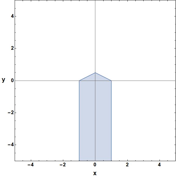
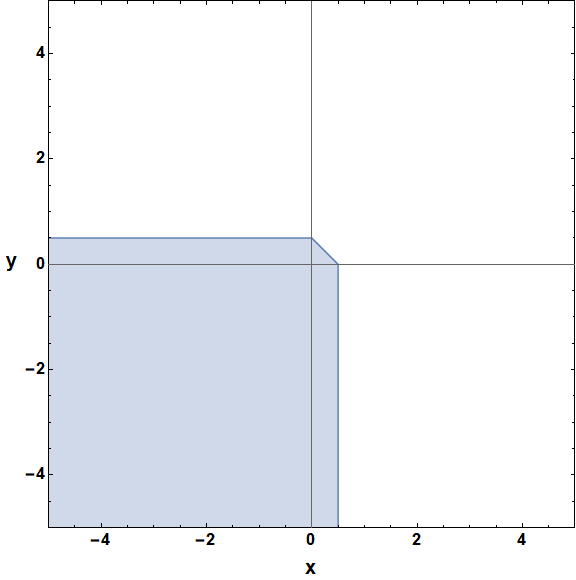
Figure 9: Convergence regions of $S_{1}$ (left), $S_{2}$ (middle) and $S_{3}$ (right) for real values of $x$ and $y$.

Series representation $S_{4}$

$S_{4}$ is obtained by applying Eq.(26) on the first Euler transformation of $F_{2}$ (first line of Eq.(6), i.e. $S_{2}$).

$$S_{4} =(1-x)^{-a}\left\langle\left(\frac{1}{1-x}\right)^{-a+b_{1}}\right\rangle\frac{\Gamma(c_{1})\Gamma(a-b_{1})}{\Gamma(a)\Gamma(c_{1}-b_{1})}\tilde{F}{}^{1:1;2}_{1:0;1}\left[\begin{array}[]{c@{{}:{}}c@{;{}}c}c_{1}-a&b_{1}&b_{2},a-c_{1}+1\\[4.30554pt] b_{1}-a+1&-&c_{2}\end{array}\;\middle|\;\frac{1}{1-x},y\right]$$ (97)

$$+(1-x)^{-a}\frac{\Gamma(c_{1})\Gamma(b_{1}-a)}{\Gamma(b_{1})\Gamma(c_{1}-a)}{F}{}^{1:1;2}_{1:0;1}\left[\begin{array}[]{c@{{}:{}}c@{;{}}c}a&c_{1}-b_{1}&b_{2},a-c_{1}+1\\[4.30554pt] a-b_{1}+1&-&c_{2}\end{array}\;\middle|\;\frac{1}{1-x},\frac{y}{1-x}\right]$$ (100)

Region of convergence: $|1-x|>1\land|y|<1$ (see Fig. 10 left).

Series representation $S_{5}$

$S_{5}$ is obtained by applying Eq.(26) on the second Euler transformation of $F_{2}$ (second line of Eq.(6)).

$$S_{5} =(1-y)^{-a}\frac{\Gamma(c_{1})\Gamma(-a-b_{1}+c_{1})}{\Gamma(c_{1}-a)\Gamma(c_{1}-b_{1})}{F}{}^{1:1;2}_{1:0;1}\left[\begin{array}[]{c@{{}:{}}c@{;{}}c}a&b_{1}&c_{2}-b_{2},a-c_{1}+1\\[4.30554pt] a+b_{1}-c_{1}+1&-&c_{2}\end{array}\;\middle|\;\frac{x+y-1}{y-1},\frac{y}{y-1}\right]$$ (103)

$$+(1-y)^{-a}\left\langle\left(\frac{x+y-1}{y-1}\right)^{-a-b_{1}+c_{1}}\right\rangle\frac{\Gamma(c_{1})\Gamma(a+b_{1}-c_{1})}{\Gamma(a)\Gamma(b_{1})}$$

$$\times\tilde{F}{}^{1:1;2}_{1:0;1}\left[\begin{array}[]{c@{{}:{}}c@{;{}}c}c_{1}-a&c_{1}-b_{1}&c_{2}-b_{2},a-c_{1}+1\\[4.30554pt] -a-b_{1}+c_{1}+1&-&c_{2}\end{array}\;\middle|\;\frac{x+y-1}{y-1},\frac{y}{x+y-1}\right]$$ (106)

Region of convergence: $|\frac{y}{x+y-1}|<1\land|\frac{x+y-1}{y-1}|<1$ (see Fig. 10 middle).

Series representation $S_{6}$

$S_{6}$ is Eq.(41).

$$S_{6} =\frac{\Gamma(c_{2})\Gamma(-a-b_{2}+c_{2})}{\Gamma(c_{2}-a)\Gamma(c_{2}-b_{2})}{F}{}^{1:2;1}_{1:1;0}\left[\begin{array}[]{c@{{}:{}}c@{;{}}c}a&a-c_{2}+1,b_{1}&b_{2}\\[4.30554pt] a+b_{2}-c_{2}+1&c_{1}&-\end{array}\;\middle|\;x,1-y\right]$$ (109)

$$+(1-y)^{-a-b_{2}+c_{2}}\left\langle\left(\frac{x}{y-1}\right)^{-a-b_{2}+c_{2}}\right\rangle\frac{\Gamma(c_{1})\Gamma(c_{2})\Gamma(a+b_{2}-c_{2})\Gamma(-a+b_{1}-b_{2}+c_{2})}{\Gamma(a)\Gamma(b_{1})\Gamma(b_{2})\Gamma(-a-b_{2}+c_{1}+c_{2})}$$

$$\times\tilde{F}{}^{2:1;1}_{2:0;0}\left[\begin{array}[]{c@{{}:{}}c@{;{}}c}a+b_{2}-c_{2},a+b_{2}-c_{2}-c_{1}+1&b_{2}&c_{2}-b_{2}\\[4.30554pt] b_{2},a-b_{1}+b_{2}-c_{2}+1&-&-\end{array}\;\middle|\;\frac{1-y}{x},x\right]$$ (112)

$$+\left\langle\left(\frac{x}{y-1}\right)^{-b_{1}}\right\rangle(1-y)^{-a-b_{2}+c_{2}}\frac{\Gamma(c_{1})\Gamma(c_{2})\Gamma(a-b_{1}+b_{2}-c_{2})}{\Gamma(a)\Gamma(b_{2})\Gamma(c_{1}-b_{1})}$$

$$\times{F}{}^{1:2;1}_{1:1;0}\left[\begin{array}[]{c@{{}:{}}c@{;{}}c}-a+b_{1}+c_{2}&b_{1},b_{1}-c_{1}+1&c_{2}-b_{2}\\[4.30554pt] -a+b_{1}-b_{2}+c_{2}+1&-a+b_{1}+c_{2}&-\end{array}\;\middle|\;\frac{1-y}{x},1-y\right]$$ (115)

Region of convergence: $|\frac{1-y}{x}|<1\land|x|<1$ (see Fig. 10 right).

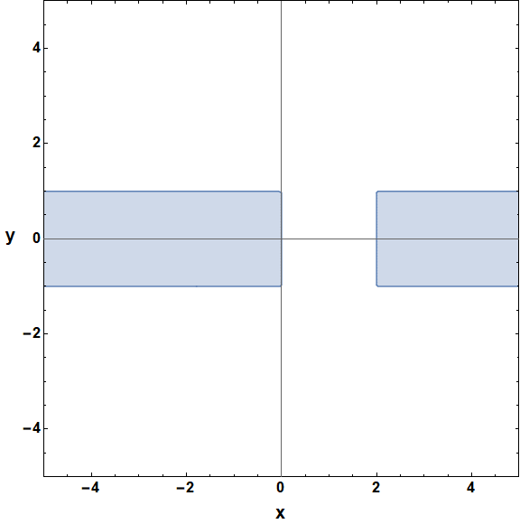
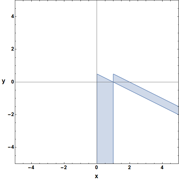
Figure 10: Convergence regions of $S_{4}$ (left), $S_{5}$ (middle) and $S_{6}$ (right) for real values of $x$ and $y$.

Series representation $S_{7}$

$S_{7}$ is obtained by applying Eq.(41), i.e. $S_{6}$, on the first Euler transformation of $F_{2}$ (first line of Eq.(6), i.e. $S_{2}$).

$$S_{7} =(1-x)^{-a}\frac{\Gamma(c_{2})\Gamma(-a-b_{2}+c_{2})}{\Gamma(c_{2}-a)\Gamma(c_{2}-b_{2})}{F}{}^{1:2;1}_{1:1;0}\left[\begin{array}[]{c@{{}:{}}c@{;{}}c}a&a-c_{2}+1,c_{1}-b_{1}&b_{2}\\[4.30554pt] a+b_{2}-c_{2}+1&c_{1}&-\end{array}\;\middle|\;\frac{x}{x-1},\frac{x+y-1}{x-1}\right]$$ (118)

$$+(1-x)^{-a}\left\langle\left(-\frac{x}{x+y-1}\right)^{-a-b_{2}+c_{2}}\right\rangle\left\langle\left(\frac{x+y-1}{x-1}\right)^{-a-b_{2}+c_{2}}\right\rangle\frac{\Gamma(c_{1})\Gamma(c_{2})\Gamma(a+b_{2}-c_{2})}{\Gamma(a)\Gamma(b_{2})\Gamma(c_{1}-b_{1})}$$

$$\times\frac{\Gamma(-a-b_{1}-b_{2}+c_{1}+c_{2})}{\Gamma(-a-b_{2}+c_{1}+c_{2})}\tilde{F}{}^{2:1;1}_{2:0;0}\left[\begin{array}[]{c@{{}:{}}c@{;{}}c}a+b_{2}-c_{2},a+b_{2}-c_{1}-c_{2}+1&b_{2}&c_{2}-b_{2}\\[4.30554pt] a+b_{1}+b_{2}-c_{1}-c_{2}+1,b_{2}&-&-\end{array}\;\middle|\;\frac{x+y-1}{x},\frac{x}{x-1}\right]$$ (121)

$$+(1-x)^{-a}\left\langle\left(\frac{x+y-1}{x-1}\right)^{-a-b_{2}+c_{2}}\right\rangle\left\langle\left(-\frac{x}{x+y-1}\right)^{b_{1}-c_{1}}\right\rangle\frac{\Gamma(c_{1})\Gamma(c_{2})\Gamma(a+b_{1}+b_{2}-c_{1}-c_{2})}{\Gamma(a)\Gamma(b_{1})\Gamma(b_{2})}$$

$$\times{F}{}^{1:2;1}_{1:1;0}\left[\begin{array}[]{c@{{}:{}}c@{;{}}c}-a-b_{1}+c_{1}+c_{2}&1-b_{1},c_{1}-b_{1}&c_{2}-b_{2}\\[4.30554pt] -a-b_{1}-b_{2}+c_{1}+c_{2}+1&-a-b_{1}+c_{1}+c_{2}&-\end{array}\;\middle|\;\frac{x+y-1}{x},\frac{x+y-1}{x-1}\right]$$ (124)

Region of convergence: $|\frac{x+y-1}{x}|<1\land|\frac{x}{x-1}|<1$ (see Fig. 11 left).

Series representation $S_{8}$

$S_{8}$ is obtained by applying Eq.(41), i.e. $S_{6}$, on the third Euler transformation of $F_{2}$ (third line of Eq.(6), i.e. $S_{3}$).

$$S_{8} =(-x-y+1)^{-a}\left\langle\left(-\frac{x}{x-1}\right)^{b_{2}-a}\right\rangle\left\langle\left(\frac{x-1}{x+y-1}\right)^{b_{2}-a}\right\rangle\frac{\Gamma(c_{1})\Gamma(c_{2})\Gamma(a-b_{2})\Gamma(-a-b_{1}+b_{2}+c_{1})}{\Gamma(a)\Gamma(c_{1}-b_{1})\Gamma(c_{2}-b_{2})\Gamma(-a+b_{2}+c_{1})}$$

$$\times\tilde{F}{}^{2:1;1}_{2:0;0}\left[\begin{array}[]{c@{{}:{}}c@{;{}}c}a-b_{2},a-b_{2}-c_{1}+1&c_{2}-b_{2}&b_{2}\\[4.30554pt] c_{2}-b_{2},a+b_{1}-b_{2}-c_{1}+1&-&-\end{array}\;\middle|\;\frac{x-1}{x},\frac{x}{x+y-1}\right]$$ (127)

$$+(-x-y+1)^{-a}\frac{\Gamma(c_{2})\Gamma(b_{2}-a)}{\Gamma(b_{2})\Gamma(c_{2}-a)}{F}{}^{1:2;1}_{1:1;0}\left[\begin{array}[]{c@{{}:{}}c@{;{}}c}a&a-c_{2}+1,c_{1}-b_{1}&c_{2}-b_{2}\\[4.30554pt] a-b_{2}+1&c_{1}&-\end{array}\;\middle|\;\frac{x}{x+y-1},\frac{x-1}{x+y-1}\right]$$ (130)

$$+(-x-y+1)^{-a}\left\langle\left(-\frac{x}{x-1}\right)^{b_{1}-c_{1}}\right\rangle\left\langle\left(\frac{x-1}{x+y-1}\right)^{b_{2}-a}\right\rangle\frac{\Gamma(c_{1})\Gamma(c_{2})\Gamma(a+b_{1}-b_{2}-c_{1})}{\Gamma(a)\Gamma(b_{1})\Gamma(c_{2}-b_{2})}$$

$$\times{F}{}^{1:2;1}_{1:1;0}\left[\begin{array}[]{c@{{}:{}}c@{;{}}c}-a-b_{1}+c_{1}+c_{2}&1-b_{1},c_{1}-b_{1}&b_{2}\\[4.30554pt] -a-b_{1}+b_{2}+c_{1}+1&-a-b_{1}+c_{1}+c_{2}&-\end{array}\;\middle|\;\frac{x-1}{x},\frac{x-1}{x+y-1}\right]$$ (133)

Region of convergence: $|\frac{x-1}{x}|<1\land|\frac{x}{x+y-1}|<1$ (see Fig. 9 middle).

Series representation $S_{9}$

$S_{9}$ is the symmetrical partner of Eq.(41) obtained from Eq.(5).

$$S_{9} =(1-x)^{-a-b_{1}+c_{1}}\left\langle\left(\frac{y}{x-1}\right)^{-b_{2}}\right\rangle\frac{\Gamma(c_{1})\Gamma(c_{2})\Gamma(a+b_{1}-b_{2}-c_{1})}{\Gamma(a)\Gamma(b_{1})\Gamma(c_{2}-b_{2})}$$

$$\times{F}{}^{1:1;2}_{1:0;1}\left[\begin{array}[]{c@{{}:{}}c@{;{}}c}-a+b_{2}+c_{1}&c_{1}-b_{1}&b_{2},b_{2}-c_{2}+1\\[4.30554pt] -a-b_{1}+b_{2}+c_{1}+1&-&-a+b_{2}+c_{1}\end{array}\;\middle|\;1-x,\frac{1-x}{y}\right]$$ (136)

$$+(1-x)^{-a-b_{1}+c_{1}}\left\langle\left(\frac{y}{x-1}\right)^{-a-b_{1}+c_{1}}\right\rangle\frac{\Gamma(c_{1})\Gamma(c_{2})\Gamma(a+b_{1}-c_{1})\Gamma(-a-b_{1}+b_{2}+c_{1})}{\Gamma(a)\Gamma(b_{1})\Gamma(b_{2})\Gamma(-a-b_{1}+c_{1}+c_{2})}$$

$$\times\tilde{F}{}^{2:1;1}_{2:0;0}\left[\begin{array}[]{c@{{}:{}}c@{;{}}c}1-b_{1},-a-b_{1}+b_{2}+c_{1}&c_{1}-b_{1}&b_{1}\\[4.30554pt] -a-b_{1}+c_{1}+1,-a-b_{1}+c_{1}+c_{2}&-&-\end{array}\;\middle|\;y,\frac{1-x}{y}\right]$$ (139)

$$+\frac{\Gamma(c_{1})\Gamma(-a-b_{1}+c_{1})}{\Gamma(c_{1}-a)\Gamma(c_{1}-b_{1})}{F}{}^{1:1;2}_{1:0;1}\left[\begin{array}[]{c@{{}:{}}c@{;{}}c}a&b_{1}&b_{2},a-c_{1}+1\\[4.30554pt] a+b_{1}-c_{1}+1&-&c_{2}\end{array}\;\middle|\;1-x,y\right]$$ (142)

Region of convergence: $|\frac{1-x}{y}|<1\land|y|<1$ (see Fig. 11 right).

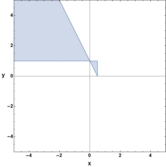
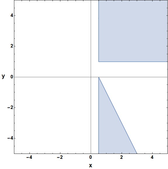
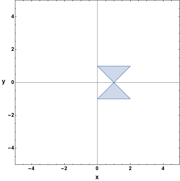
Figure 11: Convergence regions of $S_{7}$ (left), $S_{8}$ (middle) and $S_{9}$ (right) for real values of $x$ and $y$.

Series representation $S_{10}$

$S_{10}$ is obtained by applying the symmetrical partner Eq.(41), i.e. $S_{9}$, on the second Euler transformation of $F_{2}$ (second line of Eq.(6)).

$$S_{10} =(1-y)^{-a}\left\langle\left(-\frac{y}{x+y-1}\right)^{-a-b_{1}+c_{1}}\right\rangle\left\langle\left(\frac{x+y-1}{y-1}\right)^{-a-b_{1}+c_{1}}\right\rangle\frac{\Gamma(c_{1})\Gamma(c_{2})\Gamma(a+b_{1}-c_{1})}{\Gamma(a)\Gamma(b_{1})\Gamma(c_{2}-b_{2})}$$

$$\times\frac{\Gamma(-a-b_{1}-b_{2}+c_{1}+c_{2})}{\Gamma(-a-b_{1}+c_{1}+c_{2})}\tilde{F}{}^{2:1;1}_{2:0;0}\left[\begin{array}[]{c@{{}:{}}c@{;{}}c}1-b_{1},-a-b_{1}-b_{2}+c_{1}+c_{2}&c_{1}-b_{1}&b_{1}\\[4.30554pt] -a-b_{1}+c_{1}+1,-a-b_{1}+c_{1}+c_{2}&-&-\end{array}\;\middle|\;\frac{y}{y-1},\frac{x+y-1}{y}\right]$$ (145)

$$+(1-y)^{-a}\frac{\Gamma(c_{1})\Gamma(-a-b_{1}+c_{1})}{\Gamma(c_{1}-a)\Gamma(c_{1}-b_{1})}{F}{}^{1:1;2}_{1:0;1}\left[\begin{array}[]{c@{{}:{}}c@{;{}}c}a&b_{1}&a-c_{1}+1,c_{2}-b_{2}\\[4.30554pt] a+b_{1}-c_{1}+1&-&c_{2}\end{array}\;\middle|\;\frac{x+y-1}{y-1},\frac{y}{y-1}\right]$$ (148)

$$+(1-y)^{-a}\left\langle\left(\frac{x+y-1}{y-1}\right)^{-a-b_{1}+c_{1}}\right\rangle\left\langle\left(-\frac{y}{x+y-1}\right)^{b_{2}-c_{2}}\right\rangle\frac{\Gamma(c_{1})\Gamma(c_{2})\Gamma(a+b_{1}+b_{2}-c_{1}-c_{2})}{\Gamma(a)\Gamma(b_{1})\Gamma(b_{2})}$$

$$\times{F}{}^{1:1;2}_{1:0;1}\left[\begin{array}[]{c@{{}:{}}c@{;{}}c}-a-b_{2}+c_{1}+c_{2}&c_{1}-b_{1}&1-b_{2},c_{2}-b_{2}\\[4.30554pt] -a-b_{1}-b_{2}+c_{1}+c_{2}+1&-&-a-b_{2}+c_{1}+c_{2}\end{array}\;\middle|\;\frac{x+y-1}{y-1},\frac{x+y-1}{y}\right]$$ (151)

Region of convergence: $|\frac{x+y-1}{y}|<1\land|\frac{y}{y-1}|<1$ (see Fig. 12 left).

Series representation $S_{11}$

$S_{11}$ is obtained by applying the symmetrical partner Eq.(41), i.e. $S_{9}$, on the third Euler transformation of $F_{2}$ (third line of Eq.(6), i.e. $S_{3}$).

$$S_{11} =(-x-y+1)^{-a}\left\langle\left(\frac{y}{1-y}\right)^{b_{1}-a}\right\rangle\left\langle\left(\frac{y-1}{x+y-1}\right)^{b_{1}-a}\right\rangle\frac{\Gamma(c_{1})\Gamma(c_{2})\Gamma(a-b_{1})\Gamma(-a+b_{1}-b_{2}+c_{2})}{\Gamma(a)\Gamma(c_{1}-b_{1})\Gamma(c_{2}-b_{2})\Gamma(-a+b_{1}+c_{2})}$$

$$\times\tilde{F}{}^{2:1;1}_{2:0;0}\left[\begin{array}[]{c@{{}:{}}c@{;{}}c}b_{1}-c_{1}+1,-a+b_{1}-b_{2}+c_{2}&b_{1}&c_{1}-b_{1}\\[4.30554pt] -a+b_{1}+1,-a+b_{1}+c_{2}&-&-\end{array}\;\middle|\;\frac{y}{x+y-1},\frac{y-1}{y}\right]$$ (154)

$$+(-x-y+1)^{-a}\frac{\Gamma(c_{1})\Gamma(b_{1}-a)}{\Gamma(b_{1})\Gamma(c_{1}-a)}{F}{}^{1:1;2}_{1:0;1}\left[\begin{array}[]{c@{{}:{}}c@{;{}}c}a&c_{1}-b_{1}&a-c_{1}+1,c_{2}-b_{2}\\[4.30554pt] a-b_{1}+1&-&c_{2}\end{array}\;\middle|\;\frac{y-1}{x+y-1},\frac{y}{x+y-1}\right]$$ (157)

$$+(-x-y+1)^{-a}\left\langle\left(\frac{y}{1-y}\right)^{b_{2}-c_{2}}\right\rangle\left\langle\left(\frac{y-1}{x+y-1}\right)^{b_{1}-a}\right\rangle\frac{\Gamma(c_{1})\Gamma(c_{2})\Gamma(a-b_{1}+b_{2}-c_{2})}{\Gamma(a)\Gamma(b_{2})\Gamma(c_{1}-b_{1})}$$

$$\times{F}{}^{1:1;2}_{1:0;1}\left[\begin{array}[]{c@{{}:{}}c@{;{}}c}-a-b_{2}+c_{1}+c_{2}&b_{1}&1-b_{2},c_{2}-b_{2}\\[4.30554pt] -a+b_{1}-b_{2}+c_{2}+1&-&-a-b_{2}+c_{1}+c_{2}\end{array}\;\middle|\;\frac{y-1}{x+y-1},\frac{y-1}{y}\right]$$ (160)

Region of convergence: $|\frac{y-1}{y}|<1\land|\frac{y}{x+y-1}|<1$ (see Fig. 12 middle).

Series representation $S_{12}$

$S_{12}$ is Eq.(85).

$$S_{12} =(-x)^{-a}\frac{\Gamma(c_{1})\Gamma(b_{1}-a)}{\Gamma(b_{1})\Gamma(c_{1}-a)}{F}{}^{2:1;1}_{2:0;0}\left[\begin{array}[]{c@{{}:{}}c@{;{}}c}a,a-c_{1}+1&c_{2}-b_{2}&b_{2}\\[4.30554pt] c_{2},a-b_{1}+1&-&-\end{array}\;\middle|\;\frac{1}{x},\frac{1-y}{x}\right]$$ (163)

$$+(-x)^{-b_{1}}\frac{\Gamma(c_{1})\Gamma(c_{2})\Gamma(a-b_{1})\Gamma(-a+b_{1}-b_{2}+c_{2})}{\Gamma(a)\Gamma(c_{1}-b_{1})\Gamma(c_{2}-b_{2})\Gamma(-a+b_{1}+c_{2})}\tilde{F}{}^{1:2;1}_{1:1;0}\left[\begin{array}[]{c@{{}:{}}c@{;{}}c}-a+b_{1}-b_{2}+c_{2}&b_{1},b_{1}-c_{1}+1&b_{2}\\[4.30554pt] -a+b_{1}+1&-a+b_{1}+c_{2}&-\end{array}\;\middle|\;\frac{1}{x},1-y\right]$$ (166)

$$+(-x)^{-b_{1}}(1-y)^{-a+b_{1}-b_{2}+c_{2}}\frac{\Gamma(c_{1})\Gamma(c_{2})\Gamma(a-b_{1}+b_{2}-c_{2})}{\Gamma(a)\Gamma(b_{2})\Gamma(c_{1}-b_{1})}$$

$$\times{F}{}^{1:2;1}_{1:1;0}\left[\begin{array}[]{c@{{}:{}}c@{;{}}c}-a+b_{1}+c_{2}&b_{1},b_{1}-c_{1}+1&c_{2}-b_{2}\\[4.30554pt] -a+b_{1}-b_{2}+c_{2}+1&-a+b_{1}+c_{2}&-\end{array}\;\middle|\;\frac{1-y}{x},1-y\right]$$ (169)

Region of convergence: $|\frac{1}{x}|<1\land|1-y|<1$ (see Fig. 12 right).

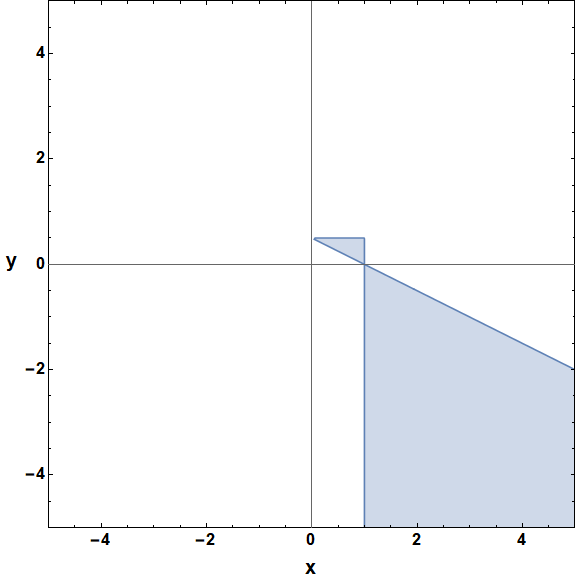
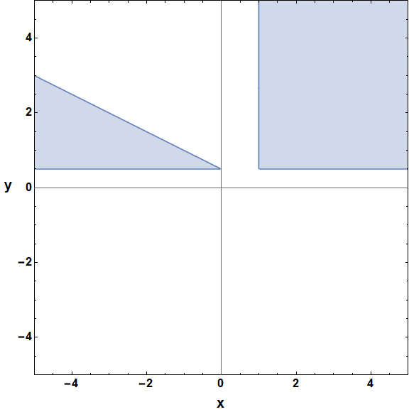
Figure 12: Convergence regions of $S_{10}$ (left), $S_{11}$ (middle) and $S_{12}$ (right) for real values of $x$ and $y$.

Series representation $S_{13}$

$S_{13}$ is obtained by applying Eq.(85), i.e. $S_{13}$, on the first Euler transformation of $F_{2}$ (first line of Eq.(6), i.e. $S_{2}$).

$$S_{13} =(1-x)^{-a}\left\langle\left(-\frac{x}{x-1}\right)^{-a}\right\rangle\frac{\Gamma(c_{1})\Gamma(-a-b_{1}+c_{1})}{\Gamma(c_{1}-a)\Gamma(c_{1}-b_{1})}{F}{}^{2:1;1}_{2:0;0}\left[\begin{array}[]{c@{{}:{}}c@{;{}}c}a,a-c_{1}+1&c_{2}-b_{2}&b_{2}\\[4.30554pt] c_{2},a+b_{1}-c_{1}+1&-&-\end{array}\;\middle|\;\frac{x-1}{x},\frac{x+y-1}{x}\right]$$ (172)

$$+(1-x)^{-a}\left\langle\left(-\frac{x}{x-1}\right)^{b_{1}-c_{1}}\right\rangle\frac{\Gamma(c_{1})\Gamma(c_{2})\Gamma(a+b_{1}-c_{1})\Gamma(-a-b_{1}-b_{2}+c_{1}+c_{2})}{\Gamma(a)\Gamma(b_{1})\Gamma(c_{2}-b_{2})\Gamma(-a-b_{1}+c_{1}+c_{2})}$$

$$\times\tilde{F}{}^{1:2;1}_{1:1;0}\left[\begin{array}[]{c@{{}:{}}c@{;{}}c}-a-b_{1}-b_{2}+c_{1}+c_{2}&1-b_{1},c_{1}-b_{1}&b_{2}\\[4.30554pt] -a-b_{1}+c_{1}+1&-a-b_{1}+c_{1}+c_{2}&-\end{array}\;\middle|\;\frac{x-1}{x},\frac{x+y-1}{x-1}\right]$$ (175)

$$+(1-x)^{-a}\left\langle\left(-\frac{x}{x-1}\right)^{b_{1}-c_{1}}\right\rangle\left\langle\left(\frac{x+y-1}{x-1}\right)^{-a-b_{1}-b_{2}+c_{1}+c_{2}}\right\rangle\frac{\Gamma(c_{1})\Gamma(c_{2})\Gamma(a+b_{1}+b_{2}-c_{1}-c_{2})}{\Gamma(a)\Gamma(b_{1})\Gamma(b_{2})}$$

$$\times{F}{}^{1:2;1}_{1:1;0}\left[\begin{array}[]{c@{{}:{}}c@{;{}}c}-a-b_{1}+c_{1}+c_{2}&1-b_{1},c_{1}-b_{1}&c_{2}-b_{2}\\[4.30554pt] -a-b_{1}-b_{2}+c_{1}+c_{2}+1&-a-b_{1}+c_{1}+c_{2}&-\end{array}\;\middle|\;\frac{x+y-1}{x},\frac{x+y-1}{x-1}\right]$$ (178)

Region of convergence: $|\frac{x-1}{x}|<1\land|\frac{x+y-1}{x-1}|<1$ (see Fig. 13 left).

Series representation $S_{14}$

$S_{14}$ is the symmetrical partner of Eq.(85) obtained from Eq.(5).

$$S_{14} =(-y)^{-a}\frac{\Gamma(c_{2})\Gamma(b_{2}-a)}{\Gamma(b_{2})\Gamma(c_{2}-a)}{F}{}^{2:1;1}_{2:0;0}\left[\begin{array}[]{c@{{}:{}}c@{;{}}c}a,a-c_{2}+1&b_{1}&c_{1}-b_{1}\\[4.30554pt] c_{1},a-b_{2}+1&-&-\end{array}\;\middle|\;\frac{1-x}{y},\frac{1}{y}\right]$$ (181)

$$+(-y)^{-b_{2}}\frac{\Gamma(c_{1})\Gamma(c_{2})\Gamma(a-b_{2})\Gamma(-a-b_{1}+b_{2}+c_{1})}{\Gamma(a)\Gamma(c_{1}-b_{1})\Gamma(c_{2}-b_{2})\Gamma(-a+b_{2}+c_{1})}\tilde{F}{}^{1:1;2}_{1:0;1}\left[\begin{array}[]{c@{{}:{}}c@{;{}}c}a-b_{2}&b_{1}&b_{2},b_{2}-c_{2}+1\\[4.30554pt] a+b_{1}-b_{2}-c_{1}+1&-&-a+b_{2}+c_{1}\end{array}\;\middle|\;1-x,\frac{1}{y}\right]$$ (184)

$$+(-y)^{-b_{2}}(1-x)^{-a-b_{1}+b_{2}+c_{1}}\frac{\Gamma(c_{1})\Gamma(c_{2})\Gamma(a+b_{1}-b_{2}-c_{1})}{\Gamma(a)\Gamma(b_{1})\Gamma(c_{2}-b_{2})}$$

$$\times{F}{}^{1:1;2}_{1:0;1}\left[\begin{array}[]{c@{{}:{}}c@{;{}}c}-a+b_{2}+c_{1}&c_{1}-b_{1}&b_{2},b_{2}-c_{2}+1\\[4.30554pt] -a-b_{1}+b_{2}+c_{1}+1&-&-a+b_{2}+c_{1}\end{array}\;\middle|\;1-x,\frac{1-x}{y}\right]$$ (187)

Region of convergence: $|1-x|<1\land|y|>1$ (see Fig. 13 middle).

Series representation $S_{15}$

$S_{15}$ is obtained by applying the symmetrical partner of Eq.(85), i.e. $S_{14}$, on the second Euler transformation of $F_{2}$ (second line of Eq.(6)).

$$S_{15} =(1-y)^{-a}\left\langle\left(-\frac{y}{y-1}\right)^{-a}\right\rangle\frac{\Gamma(c_{2})\Gamma(-a-b_{2}+c_{2})}{\Gamma(c_{2}-a)\Gamma(c_{2}-b_{2})}{F}{}^{2:1;1}_{2:0;0}\left[\begin{array}[]{c@{{}:{}}c@{;{}}c}a,a-c_{2}+1&b_{1}&c_{1}-b_{1}\\[4.30554pt] c_{1},a+b_{2}-c_{2}+1&-&-\end{array}\;\middle|\;\frac{x+y-1}{y},\frac{y-1}{y}\right]$$ (190)

$$+(1-y)^{-a}\left\langle\left(-\frac{y}{y-1}\right)^{b_{2}-c_{2}}\right\rangle\frac{\Gamma(c_{1})\Gamma(c_{2})\Gamma(a+b_{2}-c_{2})\Gamma(-a-b_{1}-b_{2}+c_{1}+c_{2})}{\Gamma(a)\Gamma(b_{2})\Gamma(c_{1}-b_{1})\Gamma(-a-b_{2}+c_{1}+c_{2})}$$

$$\times\tilde{F}{}^{1:1;2}_{1:0;1}\left[\begin{array}[]{c@{{}:{}}c@{;{}}c}a+b_{2}-c_{2}&b_{1}&1-b_{2},c_{2}-b_{2}\\[4.30554pt] a+b_{1}+b_{2}-c_{1}-c_{2}+1&-&-a-b_{2}+c_{1}+c_{2}\end{array}\;\middle|\;\frac{x+y-1}{y-1},\frac{y-1}{y}\right]$$ (193)

$$+(1-y)^{-a}\left\langle\left(-\frac{y}{y-1}\right)^{b_{2}-c_{2}}\right\rangle\left\langle\left(\frac{y-1}{x+y-1}\right)^{a+b_{1}+b_{2}-c_{1}-c_{2}}\right\rangle\frac{\Gamma(c_{1})\Gamma(c_{2})\Gamma(a+b_{1}+b_{2}-c_{1}-c_{2})}{\Gamma(a)\Gamma(b_{1})\Gamma(b_{2})}$$

$$\times{F}{}^{1:1;2}_{1:0;1}\left[\begin{array}[]{c@{{}:{}}c@{;{}}c}-a-b_{2}+c_{1}+c_{2}&c_{1}-b_{1}&1-b_{2},c_{2}-b_{2}\\[4.30554pt] -a-b_{1}-b_{2}+c_{1}+c_{2}+1&-&-a-b_{2}+c_{1}+c_{2}\end{array}\;\middle|\;\frac{x+y-1}{y-1},\frac{x+y-1}{y}\right]$$ (196)

Region of convergence: $|\frac{y-1}{y}|<1\land|\frac{x+y-1}{y-1}|<1$ (see Fig. 13 right).

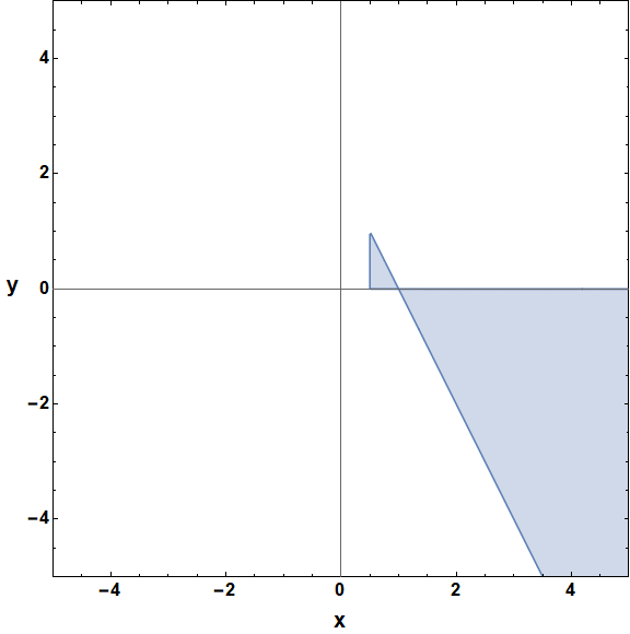
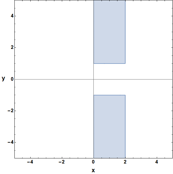
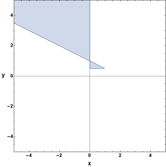
Figure 13: Convergence regions of $S_{13}$ (left), $S_{14}$ (middle) and $S_{15}$ (right) for real values of $x$ and $y$.

Series representation $S_{16}$

$S_{16}$ is obtained by applying the symmetrical partner of Eq.(85), i.e. $S_{14}$, on the third Euler transformation of $F_{2}$ (third line of Eq.(6), i.e. $S_{3}$).

$$S_{16} =(-x-y+1)^{-a}\left\langle\left(-\frac{y}{x+y-1}\right)^{-a}\right\rangle\frac{\Gamma(c_{2})\Gamma(-a-b_{2}+c_{2})}{\Gamma(c_{2}-a)\Gamma(c_{2}-b_{2})}$$

$$\times{F}{}^{2:1;1}_{2:0;0}\left[\begin{array}[]{c@{{}:{}}c@{;{}}c}a,a-c_{2}+1&c_{1}-b_{1}&b_{1}\\[4.30554pt] c_{1},a+b_{2}-c_{2}+1&-&-\end{array}\;\middle|\;\frac{y-1}{y},\frac{x+y-1}{y}\right]$$ (199)

$$+(-x-y+1)^{-a}\left\langle\left(-\frac{y}{x+y-1}\right)^{b_{2}-c_{2}}\right\rangle\frac{\Gamma(c_{1})\Gamma(c_{2})\Gamma(a+b_{2}-c_{2})\Gamma(-a+b_{1}-b_{2}+c_{2})}{\Gamma(a)\Gamma(b_{1})\Gamma(b_{2})\Gamma(-a-b_{2}+c_{1}+c_{2})}$$

$$\times\tilde{F}{}^{1:1;2}_{1:0;1}\left[\begin{array}[]{c@{{}:{}}c@{;{}}c}a+b_{2}-c_{2}&c_{1}-b_{1}&1-b_{2},c_{2}-b_{2}\\[4.30554pt] a-b_{1}+b_{2}-c_{2}+1&-&-a-b_{2}+c_{1}+c_{2}\end{array}\;\middle|\;\frac{y-1}{x+y-1},\frac{x+y-1}{y}\right]$$ (202)

$$+(-x-y+1)^{-a}\left\langle\left(-\frac{y}{x+y-1}\right)^{b_{2}-c_{2}}\right\rangle\left\langle\left(\frac{y-1}{x+y-1}\right)^{-a+b_{1}-b_{2}+c_{2}}\right\rangle\frac{\Gamma(c_{1})\Gamma(c_{2})\Gamma(a-b_{1}+b_{2}-c_{2})}{\Gamma(a)\Gamma(b_{2})\Gamma(c_{1}-b_{1})}$$

$$\times{F}{}^{1:1;2}_{1:0;1}\left[\begin{array}[]{c@{{}:{}}c@{;{}}c}-a-b_{2}+c_{1}+c_{2}&b_{1}&1-b_{2},c_{2}-b_{2}\\[4.30554pt] -a+b_{1}-b_{2}+c_{2}+1&-&-a-b_{2}+c_{1}+c_{2}\end{array}\;\middle|\;\frac{y-1}{x+y-1},\frac{y-1}{y}\right]$$ (205)

Region of convergence: $|\frac{x+y-1}{y}|<1\land|\frac{y-1}{x+y-1}|<1$ (see Fig. 14 left).

Series representation $S_{17}$

$S_{17}$ is Eq.(10).

$$S_{17} =(-y)^{-a}\frac{\Gamma(c_{2})\Gamma(b_{2}-a)}{\Gamma(b_{2})\Gamma(c_{2}-a)}F{}^{2:1;0}_{1:1;0}\left[\begin{array}[]{c@{{}:{}}c@{;{}}c}a,a-c_{2}+1&b_{1}&-\\[4.30554pt] a-b_{2}+1&c_{1}&{-}\mkern-7.0mu\cleaders\hbox{$\mkern-2.0mu-\mkern-2.0mu$}\hfill\mkern-7.0mu{-}\end{array}\;\middle|\;-\frac{x}{y},\frac{1}{y}\right]$$ (208)

$$+(-y)^{-b_{2}}\frac{\Gamma(c_{2})\Gamma(a-b_{2})}{\Gamma(a)\Gamma(c_{2}-b_{2})}\,H_{2}\left(a-b_{2},b_{1},b_{2},b_{2}-c_{2}+1;c_{1};x,-\frac{1}{y}\right)$$ (209)

Region of convergence: $|x|<1\land|-\frac{1}{y}|<1\land(|x|+1)|-\frac{1}{y}|<1$ (see Fig. 14 middle).

Series representation $S_{18}$

$S_{18}$ is the symmetrical partner of Eq.(10) obtained from Eq.(5).

$$S_{18} =(-x)^{-a}\frac{\Gamma(c_{1})\Gamma(b_{1}-a)}{\Gamma(b_{1})\Gamma(c_{1}-a)}F{}^{2:1;0}_{1:1;0}\left[\begin{array}[]{c@{{}:{}}c@{;{}}c}a,a-c_{1}+1&b_{2}&-\\[4.30554pt] a-b_{1}+1&c_{2}&{-}\mkern-7.0mu\cleaders\hbox{$\mkern-2.0mu-\mkern-2.0mu$}\hfill\mkern-7.0mu{-}\end{array}\;\middle|\;-\frac{y}{x},\frac{1}{x}\right]$$ (212)

$$+(-x)^{-b_{1}}\frac{\Gamma(c_{1})\Gamma(a-b_{1})}{\Gamma(a)\Gamma(c_{1}-b_{1})}\,H_{2}\left(a-b_{1},b_{2},b_{1},b_{1}-c_{1}+1;c_{2};y,-\frac{1}{x}\right)$$ (213)

Region of convergence: $|y|<1\land\frac{1}{|x|}<1\land\frac{|y|+1}{|x|}<1$ (see Fig. 14 right).

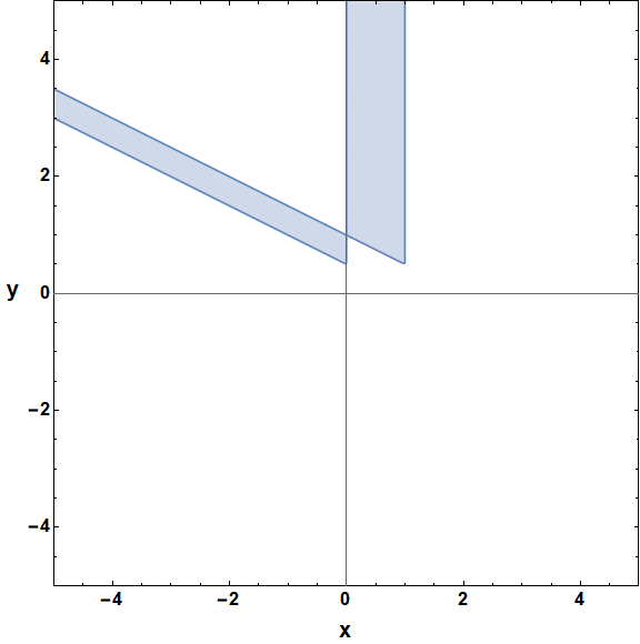
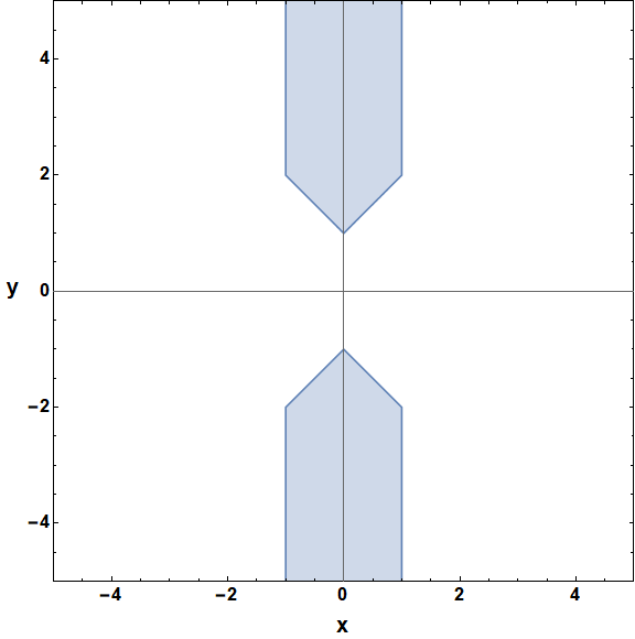
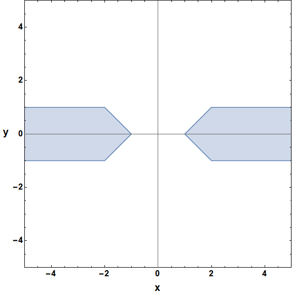
Figure 14: Convergence regions of $S_{16}$ (left), $S_{17}$ (middle) and $S_{18}$ (right) for real values of $x$ and $y$.

References

- [1] Wolfram Research, Inc., Mathematica, Version 12.3.1, Champaign, IL (2021).
- [2] Maplesoft, a division of Waterloo Maple Inc.. (2019). Maple. Waterloo, Ontario.
- [3] A. Erdelyi, W. Magnus, F. Oberhettinger and F. G. Tricomi, “Higher transcendental functions”, Bateman Project Vol. 1, McGraw-Hill Book Company (1953).
- [4] H. M. Srivastava and P. W. Karlsson “Multiple gaussian hypergeometric series”, Ellis Horwood Series in Mathematics and Its Applications, 1985.
- [5] B. Ananthanarayan, S. Banik, S. Friot and S. Ghosh, Phys. Rev. Lett. 127 (2021) no.15, 151601 doi:10.1103/PhysRevLett.127.151601 [arXiv:2012.15108 [hep-th]].
- [6] P. Appell and J. Kampé de Fériet, “Fonctions hypergéométriques et hypersphériques - Polynômes d’Hermite”, Gautiers-Villars et , 1926.
- [7] H. Exton, “Multiple hypergeometric functions and applications”, Ellis Horwood Series in Mathematics and Its Applications, 1976.
- [8] O. I. Marichev, “Handbook of integral transforms of higher transcendental functions: Theory and Algorithmic tables”, Ellis Horwood Series in Mathematics and Its Applications, 1983.
- [9] O. Zhdanov and A. Tsikh, Siberian Mathematical Journal 39, 245 (1998).
- [10] B. Ananthanarayan, S. Banik, S. Friot and S. Ghosh, Phys. Rev. D 102 (2020) no.9, 091901 doi:10.1103/PhysRevD.102.091901 [arXiv:2007.08360 [hep-th]].
- [11] B. Ananthanarayan, S. Banik, S. Friot and S. Ghosh, Phys. Rev. D 103 (2021) no.9, 096008 doi:10.1103/PhysRevD.103.096008 [arXiv:2012.15646 [hep-th]].
- [12] B. Ananthanarayan, S. Friot and S. Ghosh, Phys. Rev. D 101 (2020) no.11, 116008 doi:10.1103/PhysRevD.101.116008 [arXiv:2003.12030 [hep-ph]].
- [13] F. A. Berends, M. Buza, M. Bohm and R. Scharf, Z. Phys. C 63 (1994), 227-234 doi:10.1007/BF01411014.
- [14] B. Ananthanarayan, S. Friot and S. Ghosh, Eur. Phys. J. C 80 (2020) no.7, 606 doi:10.1140/epjc/s10052-020-8131-3 [arXiv:1911.10096 [hep-ph]].
- [15] B. Ananthanarayan, S. Friot, S. Ghosh and A. Hurier, [arXiv:2005.07170 [hep-th]].
- [16] P. O. M. Olsson, J. Math. Phys. 5, 420 (1964).
- [17] A. Erdélyi, Proc. Roy. Soc. Edinburgh Sect. A, 62 (1948), 378-385.
- [18] P. O. M. Olsson, J. Math. Phys. 18, 1285 (1977).
- [19] B. Ananthanarayan, Souvik Bera, S. Friot, O. Marichev and Tanay Pathak, work in progress.
- [20] S. Friot and D. Greynat, J. Math. Phys. 53, 023508 (2012) [arXiv:1107.0328 [math-th]].
- [21] M. Passare, A. K. Tsikh and A. A. Cheshel, Theor. Math. Phys. 109 (1997), 1544-1555 [arXiv:hep-th/9609215 [hep-th]].
- [22] V. Del Duca, C. Duhr, E. W. Nigel Glover and V. A. Smirnov, JHEP 01 (2010), 042 doi:10.1007/JHEP01(2010)042 [arXiv:0905.0097 [hep-th]].
- [23] W. Becken and P. Schmelcher, J. Comp. Appl. Math. Vol. 126, Issues 1-2, 449-478 (2000).