A $K$-function for inhomogeneous random measures with geometric features

Abstract

This paper introduces a $K$-function for assessing second-order properties of inhomogeneous random measures generated by marked point processes. The marks can be geometric objects like fibers or sets of positive volume, and the presented $K$-function takes into account geometric features of the marks, such as tangent directions of fibers. The $K$-function requires an estimate of the inhomogeneous density function of the random measure. We introduce parametric estimates for the density function based on parametric models that represent large scale features of the inhomogeneous random measure. The proposed methodology is applied to simulated fiber patterns as well as a three-dimensional data set of steel fibers in concrete.

Keywords: fiber process, germ-grain model, inhomogeneous, $K$-function, marked point process, random measure, tangent vector.

1 Introduction

The $K$-function (Ripley, 1976) continues to be a key tool for studying interactions in spatial point patterns. For a stationary point process, the $K$-function times the intensity gives for each distance the expected number of further points within that distance from a typical point. In Baddeley et al. (2000) the $K$-function was extended to inhomogeneous point processes with non-constant intensity functions but satisfying a certain second-order translational invariance (second-order intensity-reweighted stationarity). Point processes can be viewed as integer valued random measures and the $K$-function has been generalized to more general random measures corresponding to e.g. length measures for random patterns of fibers (Chiu et al., 2013) or area measures on germ-grain models with grains of positive area (Gallego et al., 2016). While the results in Chiu et al. (2013) are restricted to stationary fiber processes, Gallego et al. (2016) adopted ideas from Baddeley et al. (2000) to obtain a $K$-function for inhomogeneous random sets. Van Lieshout (2018) introduced a cross $K$-function for inhomogeneous bivariate random measures generalizing results for the stationary case in Stoyan and Ohser (1982).

The objective of the current paper is related to Gallego et al. (2016) in that we define a $K$-function for inhomogeneous random measures. The modeling framework for our results essentially corresponds to marked point process (germ-grain) models with observable marks (grains). This allows us to derive a simple expression for the proposed $K$-function under a null model of no interaction. This is in contrast to Gallego et al. (2016) who assume that only the union of grains can be observed. In some cases the assumption of observable grains is restrictive but it allows for further theoretical insight. Moreover, since 3D imaging is becoming more common, the assumption of observable grains becomes less restrictive. For instance, the overlap of objects in 2D images is often due to a planar projection of a 3D structure. While we define our $K$-function in a general setup for germ-grain type random measures, we pay special attention to the case of inhomogeneous fiber patterns.

When considering patterns of geometric objects more complex than points it is also relevant to consider local geometric features of the objects, e.g. tangent directions of fibers. Accordingly, our proposed $K$-function takes into account such geometric features. In the special case of fiber patterns, our work is related to Schwandtke (1988) who considers weighted second-order measures and reduced moment measures where the weights depend on geometric features of the fibers such as tangent directions. However, the theoretical results of Schwandtke (1988) are only obtained in a stationary setting. Similar to Gallego et al. (2016), Schwandtke (1988) considers the union of fibers where the applicability of our results relies on being able to distinguish fibers.

Our $K$-function requires knowledge of the first-order moment density of the random measure. Gallego et al. (2016) suggest kernel estimation of the density function and Van Lieshout (2018) also uses kernel estimation in the data example considered. In contrast, we construct new parametric estimators that are less susceptible to overfitting.

A different approach is considered in Hansen et al. (2021) who develop a mark-weighted $K$-function (Penttinen et al., 1992) for stationary fiber patterns. The so-called currents metric is used in Hansen et al. (2021) to measure the similarity of fibers both in terms of distance and tangent directions. This requires that fibers can be observed in their entirety. This can be a limitation due to edge effects when fibers extend outside the observation window. In contrast, in the context of fiber patterns, we only use local information and we can provide edge corrected versions of our proposed $K$-function.

Summarizing, we introduce a new $K$-function for inhomogeneous random measures with geometric features generated by germ-grain models. The $K$-function does not require knowledge of the germs and only uses local information about the grains in neighborhoods used to define the $K$-function. We also introduce novel parametric estimators for inhomogeneous first-order moment densities needed for the estimation of the $K$-function. We apply our new $K$-function to simulated data sets and a data example of a 3D fiber pattern.

2 Moment measures and $K$-function for inhomogeneous random measures with geometric features

Our basic framework for inhomogeneous random measures is a random countable collection $Z=\{m_{1},m_{2},\ldots\}$ of random measures $m_{i}$ taking values in some space $\mathbb{M}$ of finite measures on $\mathbb{R}^{d}\times\mathbb{S}$ where $\mathbb{S}$ is a metric space with metric $d_{\mathbb{S}}$. In applications, each $m_{i}$ will often be a measure associated to a geometric object in $\mathbb{R}^{d}$ with geometric features of the object represented by points in $\mathbb{S}$ as in the following example.

Example 2.1.

Let $\{\Gamma_{1},\Gamma_{2},\ldots\}$ be an oriented segment process. Each $\Gamma_{i}$ is a random line segment determined by its midpoint $u_{i}$, random direction $\Theta_{i}\in\mathbb{S}^{d-1}$, and random length $L_{i}$. Letting $\mathbb{S}=\mathbb{S}^{d-1}$ be the space of possible segment directions, there is an associated collection of random measures $\{m_{1},m_{2},\ldots\}$ given by

$$m_{i}(A\times S)=\int_{\Gamma_{i}}\mathds{1}[x\in A,\Theta_{i}\in S]\lambda(\mathrm{d}x)=\int_{-L_{i}/2}^{L_{i}/2}\mathds{1}[u_{i}+r\Theta_{i}\in A,\Theta_{i}\in S]\mathrm{d}r,$$

where $A\subseteq\mathbb{R}^{d}$, $S\subseteq\mathbb{S}$ and $\lambda$ denotes length measure on the segment.

We return to Example 2.1 in Section 3 where we also give specific constructions of $Z$. Other examples that fit our framework is when $m_{i}$ are volume measures on objects in $\mathbb{R}^{d}$ as in Gallego et al. (2016) or length measures on weighted fibers as suggested by Schwandtke (1988). The fiber case generalizes Example 2.1 and will be discussed further in Section 4.

We define a random measure $\Phi$ on $\mathbb{R}^{d}\times\mathbb{S}$ by

$$\Phi(A\times S)=\sum_{m\in Z}m(A\times S),\quad A\subseteq\mathbb{R}^{d},S\subseteq\mathbb{S}.$$ (1)

The first moment measure of $\Phi$ is

$$\mu(A\times S)={\mathbb{E}}\Phi(A\times S)$$ (2)

for $A\subseteq\mathbb{R}^{d}$ and $S\subseteq\mathbb{S}$. If $\mu$ has a density $\rho(\cdot,\cdot)$ with respect to Lebesgue measure times a reference measure $\nu$ on $\mathbb{S}$, then

$$\int_{\mathbb{R}^{d}\times\mathbb{S}}f(z,s)\mu({\rm d}z\times\mathrm{d}s) =\int_{\mathbb{R}^{d}\times\mathbb{S}}f(z,s)\rho(z,s)\mathrm{d}z\nu(\mathrm{d}s).$$

In the sequel we are going to assume that $\rho$ and hence $\mu$ are well-defined. Some examples where this is satisfied are given in Section 3.1. If $\rho(\cdot,\cdot)$ is constant we say that $\Phi$ is homogeneous and otherwise that $\Phi$ is inhomogeneous. Note that inhomogeneity can be due to spatial variation when $\rho$ varies as a function of its first argument as well as due to non-uniformity of the density $\rho(z,\cdot)$, $z\in\mathbb{R}^{d}$, as a function of the ‘geometric’ argument.

The second-order factorial type moment measure for $\Phi$ is defined as

$$\alpha^{(2)}(A\times S,B\times T)={\mathbb{E}}\sum_{m,m^{\prime}\in Z}^{\neq}m(A\times S)m^{\prime}(B\times T)$$

for $A,B\subseteq\mathbb{R}^{d}$ and $S,T\subseteq\mathbb{S}$. Here $\neq$ over the sum indicates that the sum is over pairs of distinct measures $m$ and $m^{\prime}$ in $Z$.

For simplicity of exposition, we here and in the following omit details of measurability. For example, when writing $A\subseteq\mathbb{R}^{d}$ it is understood that $A$ is a Borel measurable subset of $\mathbb{R}^{d}$. Moreover, we routinely use the standard measure-theoretical arguments that allows us to establish integral equalities involving general non-negative functions from the corresponding equalities involving indicator functions (i.e. passing from indicator functions to simple functions to increasing limits of simple functions). We use $f$ as generic notation for a non-negative measurable function where the domain of $f$ will be clear from the context.

2.1 Reweighted moment measures and $K$-function

Inspired by Baddeley et al. (2000), we consider density-reweighted versions of the first- and second-order moment measures. First note that the reweighted first-order measure

$$\mu_{w}(A\times S)={\mathbb{E}}\sum_{m\in Z}\int_{\mathbb{R}^{d}\times\mathbb{S}}\frac{\mathds{1}[x\in A,s\in S]}{\rho(x,s)}m(\mathrm{d}x\times\mathrm{d}s)$$

becomes stationary in the sense $\mu_{w}(A\times S)=\mu_{w}((A+h)\times S)$ for all $h\in\mathbb{R}^{d}$. Next, the reweighted second-order measure $\alpha^{(2)}_{w}$ is defined as

$$\alpha^{(2)}_{w}(A\times S,B\times T)$$

$$= {\mathbb{E}}\sum_{m,m^{\prime}\in Z}^{\neq}\int_{(\mathbb{R}^{d}\times\mathbb{S})^{2}}\!\!\!\!\!\!\!\!\!\frac{\mathds{1}[(x,s)\in A\times S,(y,t)\in B\times T]}{\rho(x,s)\rho(y,t)}m(\mathrm{d}x\times\mathrm{d}s)m^{\prime}(\mathrm{d}y\times\mathrm{d}t).$$ (3)

We say that $\alpha^{(2)}_{w}$ is stationary if

$$\alpha^{(2)}_{w}(A\times S,B\times T)=\alpha^{(2)}_{w}((A+h)\times S,(B+h)\times T)$$

for $h\in\mathbb{R}^{d}$. In that case a $K$-function can be defined as follows.

Definition 2.2.

For any observation window $W\subseteq\mathbb{R}^{d}$ of positive volume $|W|>0$, and $r_{1},r_{2}>0$ we define

$$K_{w}(r_{1},r_{2};W)$$ (4)

$$= \frac{1}{|W|}\mathbb{E}\!\!\!\sum_{m,m^{\prime}\in Z}^{\neq}\int_{(\mathbb{R}^{d}\times\mathbb{S})^{2}}\!\!\!\!\!\!\!\!\!\frac{\mathds{1}[x\in W,\|x-y\|\leq r_{1},d_{\mathbb{S}}(s,t)\leq r_{2}]}{\rho(x,s)\rho(y,t)}m({\rm d}x\times\mathrm{d}s)m^{\prime}({\rm d}y\times\mathrm{d}t)$$

$$= \frac{1}{|W|}\int_{W\times\mathbb{S}\times\mathbb{R}^{d}\times\mathbb{S}}\mathds{1}[\|x-y\|\leq r_{1},d_{\mathbb{S}}(s,t)\leq r_{2}]\alpha_{w}^{(2)}({\rm d}x\times{\rm d}s,{\rm d}y\times{\rm d}t).$$

If $\alpha^{(2)}_{w}$ is stationary, then $K(\cdot,\cdot;W)$ does not depend on $W$ and we define

$$K_{w}(r_{1},r_{2})=K_{w}(r_{1},r_{2};W)$$

for any choice of $W$.

In Section 3.3 below, we discuss when $\alpha_{w}^{(2)}$ is stationary and show that $K_{w}$ has a simple expression under the null model that the measures in $Z$ are independent.

Unfortunately, contrary to the case of the $K$-function for point processes, the above defined $K_{w}$ does not seem to have a simple interpretation in terms of Palm expectations. However, from the definition (4) it is clear that the $K_{w}$-function is a measure of similarity of pairs of random measures $m$ and $m^{\prime}$ in terms of spatial distance and geometric attributes of $m$ and $m^{\prime}$.

3 Results and examples based on marked point process representation

To construct specific models, it is convenient to represent $Z$ as a marked point process $X=\{(u,m)\}_{u\in Y}$ where $Y$ is a point process on $\mathbb{R}^{d}$ and the marks $m$ are the random measures in $Z$. This viewpoint is natural when $Z$ arises from a germ-grain model by letting $Y$ be the point process formed by the germs and the marks be the measures associated with the grains. For instance in Example 2.1, $Y$ would be the point process formed by the midpoints of line segments. We will often refer to the points in $Y$ as center points even if they do not need to have such an interpretation. We denote the intensity of $Y$ by $\rho_{Y}$.

In this section, we take this marked point process approach and provide details and examples regarding the moment measures $\mu$ and $\alpha^{(2)}$ and the $K_{w}$-function by exploiting properties of the marked point process $X$.

3.1 First moment measure

The first-order moment measure of the marked point process $X$ is

$$\mu_{X}(A\times F)={\mathbb{E}}\sum_{(u,m)\in X}\mathds{1}[u\in A,m\in F]$$

for $A\subseteq\mathbb{R}^{d},F\subseteq\mathbb{M}$. By disintegration we can express $\mu_{X}$ as

$$\mu_{X}(A\times F)=\int_{A}{\mathbb{E}}_{u}\mathds{1}[m\in F]\rho_{Y}(u)\mathrm{d}u,$$

where for a fixed $u$ we can view ${\mathbb{E}}_{u}$ as expectation for a marked point $(u,m)$ conditional on $u\in Y$. Then by standard arguments,

$${\mathbb{E}}\sum_{(u,m)\in X}f(u,m)=\int_{\mathbb{R}^{d}}{\mathbb{E}}_{u}f(u,m)\rho_{Y}(u)\mathrm{d}u.$$ (5)

Combining the definitions (1) and (2) of $\Phi$ and $\mu$ and (5),

$$\int_{\mathbb{R}^{d}\times\mathbb{S}}f(z,s)\mu({\rm d}z\times\mathrm{d}s) ={\mathbb{E}}\sum_{(u,m)\in X}\int_{\mathbb{R}^{d}\times\mathbb{S}}f(x,s)m(\mathrm{d}x\times\mathrm{d}s)$$

$$=\int_{\mathbb{R}^{d}}\mathbb{E}_{u}\int_{\mathbb{R}^{d}\times\mathbb{S}}f(x,s)m(\mathrm{d}x\times\mathrm{d}s)\rho_{Y}(u){\rm d}u.$$ (6)

We now explore a few examples regarding the nature of the density $\rho$.

Example 3.1.

Suppose ${\mathbb{E}}_{u}m(\cdot)$ has a density $\xi_{u}$ with respect to Lebesgue measure times $\nu$ where $\nu$ is a reference measure on $\mathbb{S}$ (e.g. surface measure when $\mathbb{S}$ is the unit sphere). Then

$${\mathbb{E}}_{u}m(A\times S)=\int_{\mathbb{R}^{d}\times\mathbb{S}}\mathds{1}[(x,s)\in A\times S]\xi_{u}(x,s)\mathrm{d}x\nu(\mathrm{d}s),\quad A\subseteq\mathbb{R}^{d},S\subseteq\mathbb{S}.$$

By (6),

$$\mu(A\times S)= \int_{\mathbb{R}^{d}\times\mathbb{R}^{d}\times\mathbb{S}}\mathds{1}[z\in A,s\in S]\xi_{u}(z,s)\mathrm{d}z\nu(\mathrm{d}s)\rho_{Y}(u)\mathrm{d}u$$

$$= \int_{\mathbb{R}^{d}\times\mathbb{S}}\mathds{1}[z\in A,s\in S]\int_{\mathbb{R}^{d}}\xi_{u}(z,s)\rho_{Y}(u)\mathrm{d}u\mathrm{d}z\nu(\mathrm{d}s)$$

meaning that $\mu$ has density

$$\rho(z,s)=\int_{\mathbb{R}^{d}}\xi_{u}(z,s)\rho_{Y}(u)\mathrm{d}u$$ (7)

with respect to Lebesgue measure times $\nu$. Note that (7) may not be finite, in which case the measure $\mu$ and density $\rho$ are not well-defined. A sufficient condition for $\rho$ to be finite is if $\rho_{Y}$ is bounded, $\xi_{u}(z,s)=\xi(z-u,s)$ for some density $\xi$ not depending on $u$, and

$$\int_{\mathbb{R}^{d}}\xi(z,s)\mathrm{d}z<\infty,\quad s\in\mathbb{S}.$$

The density $\xi_{u}$ may not always exist, as the next example shows, but a density for $\mu$ may still exist.

Example 3.2.

Consider the segment process in Example 2.1 and let $Y$ be the point process formed by segment midpoints. For a given $u\in Y$, the corresponding mark $m$ was

$$m(A\times S)=\int_{-L/2}^{L/2}\mathds{1}[u+r\Theta\in A,\Theta\in S]\mathrm{d}r.$$

Up to length, both the segment and its direction are uniquely determined by $\Theta$. Due to this degeneracy, a density for ${\mathbb{E}}_{u}$ with respect to Lebesgue measure on $\mathbb{R}^{d}$ times surface measure $\nu$ on $\mathbb{S}^{d-1}$ does not exist.

Nevertheless, assume that given $Y$, the pairs $(L_{i},\Theta_{i})$ are i.i.d. Moreover, assume that $L_{i}$ and $\Theta_{i}$ are independent and $\Theta_{i}$ has density $\eta$ with respect to $\nu$. In this case, we can still identify a density for $\mu$:

$$\rho(z,s)=\mathbb{E}\int_{-L/2}^{L/2}\eta(s)\rho_{Y}(z-rs)\mathrm{d}r.$$

Details are given in A.

3.2 Second moment measure

We define a second-order factorial type moment measure for $X$ by

$$\alpha_{X}^{(2)}(A\times F,B\times G)={\mathbb{E}}\sum_{(u,m),(u^{\prime},m^{\prime})\in X}^{\neq}\mathds{1}[u\in A,m\in F,u^{\prime}\in B,m^{\prime}\in G]$$

for $A,B\subseteq\mathbb{R}^{d}$ and $F,G\subseteq\mathbb{M}$. By disintegration and assuming existence of the pair correlation function of $Y$ (e.g.  Møller and Waagepetersen, 2004), we can express $\alpha_{X}^{(2)}$ as

$$\alpha_{X}^{(2)}(A\times F,B\times G)=\int_{A\times B}\rho_{Y}(u)\rho_{Y}(u^{\prime})g_{Y}(u,u^{\prime}){\mathbb{E}}_{u,u^{\prime}}\mathds{1}[m\in F,m^{\prime}\in G]\mathrm{d}u\mathrm{d}u^{\prime},$$

where $g_{Y}$ is the pair correlation function and ${\mathbb{E}}_{u,u^{\prime}}$ can be interpreted as mean with respect to the conditional distribution of $(m,m^{\prime})$ for marked points $(u,m)$ and $(u^{\prime},m^{\prime})$ given that $u,u^{\prime}\in Y$. By standard arguments,

$${\mathbb{E}}\!\!\!\!\!\!\sum_{\begin{subarray}{c}(u,m),\\ (u^{\prime},m^{\prime})\in X\end{subarray}}^{\neq}\!\!\!\!\!\!f(u,m,u^{\prime},m^{\prime})=\int_{\mathbb{R}^{2d}}\!\!\!\!\!\!\rho_{Y}(u)\rho_{Y}(u^{\prime})g_{Y}(u,u^{\prime}){\mathbb{E}}_{u,u^{\prime}}f(u,m,u^{\prime},m^{\prime})\mathrm{d}u\mathrm{d}u^{\prime}.$$ (8)

Assume ${\mathbb{E}}_{u,u^{\prime}}m(\cdot)m^{\prime}(\cdot)$ has density $\xi_{u,u^{\prime}}$, i.e.

$${\mathbb{E}}_{u,u^{\prime}}m(A\times S)m^{\prime}(B\times T)$$

$$= \int_{(\mathbb{R}^{d}\times\mathbb{S})^{2}}\mathds{1}[(x,s)\in A\times S,(y,t)\in B\times T]\xi_{u,u^{\prime}}((x,s),(y,t))\mathrm{d}x\mathrm{d}y\nu(\mathrm{d}s)\nu(\mathrm{d}t).$$ (9)

with $\nu$ a reference measure on $\mathbb{S}$ as in the previous section. Then

$$\alpha^{(2)}(A\times S,B\times T)$$

$$= \int_{(\mathbb{R}^{d})^{2}}\rho_{Y}(u)\rho_{Y}(u^{\prime})g_{Y}(u,u^{\prime})\int_{(\mathbb{R}^{d}\times\mathbb{S})^{2}}\mathds{1}[(x,s)\in A\times S,(y,t)\in B\times T]$$

$$\xi_{u,u^{\prime}}((x,s),(y,t))\mathrm{d}x\mathrm{d}y\nu(\mathrm{d}s)\nu(\mathrm{d}t)\mathrm{d}u\mathrm{d}u^{\prime}$$

$$= \int_{(\mathbb{R}^{d}\times\mathbb{S})^{2}}\mathds{1}[(z,s)\in A\times S,(z^{\prime},t)\in B\times T]$$

$$\int_{(\mathbb{R}^{d})^{2}}\rho_{Y}(u)\rho_{Y}(u^{\prime})g_{Y}(u,u^{\prime})\xi_{u,u^{\prime}}((z,s),(z^{\prime},t))\mathrm{d}u\mathrm{d}u^{\prime}\nu(\mathrm{d}s)\nu(\mathrm{d}t)\mathrm{d}z\mathrm{d}z^{\prime}.$$

It follows that $\alpha^{(2)}$ has density

$$\rho^{(2)}(z,s,z^{\prime},t)=\int_{\mathbb{R}^{d}\times\mathbb{R}^{d}}\rho_{Y}(u)\rho_{Y}(u^{\prime})g_{Y}(u,u^{\prime})\xi_{u,u^{\prime}}((z,s),(z^{\prime},t))\mathrm{d}u\mathrm{d}u^{\prime}.$$ (10)

We return to this expression in Section 3.3.

3.3 $K$-function under null model

Consider the null model that $Y$ is Poisson and that given $Y$, the marks are independent (but not necessarily identically distributed). Then the $K$-function has a simple expression:

Proposition 3.3.

Under the null model, $\alpha^{(2)}_{w}$ is stationary and

$$K_{w}(r_{1},r_{2})=K_{0}(r_{1},r_{2}):=|b(0,r_{1})|\nu^{2}((s,t)\in\mathbb{S}\times\mathbb{S}\,|\,d_{\mathbb{S}}(s,t)\leq r_{2}).$$ (11)

Proof.

Under the null model, $g_{Y}=1$ and ${\mathbb{E}}_{u,u^{\prime}}\mathds{1}[m\in F,m^{\prime}\in G]={\mathbb{E}}_{u}\mathds{1}[m\in F]{\mathbb{E}}_{u^{\prime}}\mathds{1}[m^{\prime}\in G]$. It follows from (8) that $\alpha^{(2)}_{w}=\mu_{w}\otimes\mu_{w}$. Hence

$$K_{w}(r_{1},r_{2}){} =\frac{1}{|W|}\int_{(\mathbb{R}^{d}\times\mathbb{S})^{2}}\mathds{1}[z\in W,\|z-z^{\prime}\|\leq r_{1},d_{\mathbb{S}}(s,t)\leq r_{2}]{\rm d}z{\rm d}z^{\prime}\nu({\rm d}s)\nu({\rm d}t)$$

$$=|b(0,r_{1})|\nu^{2}((s,t)\in\mathbb{S}\times\mathbb{S}\,|\,d_{\mathbb{S}}(s,t)\leq r_{1}).$$

∎

Apart from the null model, it is hard to identify specific models for which $\alpha_{w}^{(2)}$ is stationary. Assuming that $\alpha^{(2)}$ has density $\rho^{(2)}$, we may define

$$g(z,s,z^{\prime},t)=\frac{\rho^{(2)}(z,s,z^{\prime},t)}{\rho(z,s)\rho(z^{\prime},t)}$$

as a normalized version of $\rho^{(2)}$ in the spirit of the pair correlation function of a point process. Then stationarity of $\alpha_{w}^{(2)}$ becomes equivalent to

$$g(z,s,z^{\prime},t)=g(z+h,s,z^{\prime}+h,t),\quad h\in\mathbb{R}^{d}.$$ (12)

It is not easy in general to identify specific choices of $X$ for which (12) holds due to the expressions (7) and (10) for $\rho$ and $\rho^{(2)}$ that confound properties of $Y$ and the mark conditional densities.

Remark 3.4.

In the definition (4) of $K_{w}$, the sum is only taken over pairs of distinct measures $m$ and $m^{\prime}$. Taking the sum over all pairs instead would result in an extra term in (11) which in the marked point process setup is

$$\int_{\mathbb{R}^{d}}\rho_{Y}(u)\mathbb{E}_{u}\!\int_{(\mathbb{R}^{d}\times\mathbb{S})^{2}}\frac{\mathds{1}[x\in W,\|x-y\|\leq r_{1},d_{\mathbb{S}}(s,t)\leq r_{2}]}{\rho(x,s)\rho(y,t)}m({\rm d}x\times{\rm d}s)m({\rm d}y\times{\rm d}t){\rm d}u.$$

This depends on the actual mark distribution in a non-trivial way, so we no longer get a simple expression for the $K$-function under the null model. This is a well-known problem even in the stationary case, (see e.g. Ex. 8.4 in Chiu et al., 2013). Excluding identical pairs was suggested in Jensen et al. (1990) for the stationary case. However, it has been customary to include all pairs since this avoids the computational problem of distinguishing between different marks.

Remark 3.5.

Consider the marked point process setup. Then another way of defining a reweighted $K$-function is to replace the weights $\rho(x,s)$ by $w(u,x,s)=\xi_{u}(x,s)\rho_{Y}(u)$. This results in a larger class of models for which $\alpha^{(2)}_{w}$ is stationary and the $K$-function hence is well-defined, see the discussion in B. The resulting $K$-function under the null model is the same as in (11) up to a constant that depends on the support of $\xi_{u}$. However, this choice of weights has several drawbacks. It requires that the densities $\xi_{u}$ exist and have finite support. Explicit knowledge of the center points is also required, which may cause problems e.g. if some center points lie outside the observation window. Moreover, the estimation of $\xi_{u}$ is more involved, and since values of $\xi_{u}$ far from the center point may be small, using them for the $K$-function may be numerically unstable. We therefore do not consider these weights further in this paper.

4 Specialization to fibers

The case where $X$ is defined by a fiber process is an example of special interest for our later application in Section 7. So consider a fiber process, i.e. a marked point process $\{(u,\gamma)\}_{u\in Y}$ where for a marked point $(u,\gamma)$, $\gamma$ is a finite length smooth fiber with midpoint at $u$. In the case of oriented fibers, $\mathbb{S}$ is the space $\mathbb{S}^{d-1}$ of unit vectors in $\mathbb{R}^{d}$, and for unoriented fibers, we let $\mathbb{S}$ be a hemi-sphere in $\mathbb{R}^{d}$ such that a point $s\in\mathbb{S}$ uniquely identifies a line in $\mathbb{R}^{d}$ passing through the origin. To each fiber $\gamma$, we associate the measure

$$m(A\times S)=\int_{\gamma}\mathds{1}[x\in A,\tau(x)\in S]\lambda(\mathrm{d}x)$$ (13)

where $\tau(x)\in\mathbb{S}$ is a unit tangent vector at $x$ and $\lambda$ denotes the length measure on the fiber. The tangent vector $\tau(x)$ is not uniquely defined for unoriented fibers and we simply choose the one ($\tau(x)$ or $-\tau(x)$) belonging to the hemi-sphere $\mathbb{S}$. With a slight abuse of notation we use $X$ to denote both the fiber process $\{(u,\gamma)\}_{u\in Y}$ and the marked point process $\{(u,m)\}_{u\in Y}$ with marks given by (13). For simplicity of exposition, we consider only the case of oriented fibers below, the modification to the unoriented case being straightforward.

In the oriented case, $\mathbb{S}=\mathbb{S}^{d-1}$ is a metric space with a metric $d_{\angle}$ given by the angle between unit vectors

$$d_{\angle}(\tau_{1},\tau_{2})=\arccos(\tau_{1}^{\mbox{\scriptsize\sf T}}\tau_{2})$$

for $\tau_{1},\tau_{2}\in\mathbb{S}^{d-1}$. In the unoriented case, $\mathbb{S}$ has the metric $d$ given by

$$d(\tau_{1},\tau_{2})=\min\{d_{\angle}(\tau_{1},\tau_{2}),d_{\angle}(\tau_{1},-\tau_{2})\},$$

which can be interpreted as the angle between the lines determined by $\tau_{1}$ and $\tau_{2}$. The measure $\nu$ on $\mathbb{S}$ is the surface area measure normalized so that $\nu(\mathbb{S})=1$.

The $K$-function from Section 2.1 becomes

$$K_{w}(r_{1},r_{2};W)$$

$$= \frac{1}{|W|}\mathbb{E}\sum_{\begin{subarray}{c}(u,\gamma),\\ (u^{\prime},\gamma^{\prime})\in X\end{subarray}}^{\neq}\int_{\gamma}\int_{\gamma^{\prime}}\frac{\mathds{1}[x\in W,\|x-y\|\leq r_{1},d_{\mathbb{S}}(\tau(x),\tau(y))\leq r_{2}]}{\rho(x,\tau(x))\rho(y,\tau(y))}\lambda(\mathrm{d}y)\lambda(\mathrm{d}x).$$

The value of the $K$-function under the null model is

$$K_{0}(r_{1},r_{2})=|b(0,r_{1})|\nu(\tau\in\mathbb{S}\mid d_{\mathbb{S}}(\tau,e_{1})\leq r_{2}),$$

where $e_{1}\in\mathbb{S}$ is the north pole. In the oriented case, for $d=2$,

$$K_{0}(r_{1},r_{2})=r_{1}^{2}r_{2},\quad r_{1}\geq 0,\,r_{2}\in[0,\pi],$$

and for $d=3$,

$$K_{0}(r_{1},r_{2}){} =\frac{2\pi}{3}r_{1}^{3}(1-\cos r_{2})\quad r_{1}\geq 0,\,r_{2}\in[0,\pi].$$

In the unoriented case, $K_{0}$ is twice of $K_{0}$ in the oriented case for $r_{1}\geq 0,r_{2}\in[0,\pi/2]$.

5 Estimation

In this section we discuss estimation of $K_{w}$ given an observation of $Z$ restricted to a bounded observation window $W$. We first consider the case of a known density $\rho$ and next we consider estimation of $\rho$ based on $\Phi$ restricted to $W$.

5.1 Estimation of $K_{w}$

Let $W$ be a bounded observation window of positive volume. For $m\in Z$, suppose we only observe the restriction of $m$ to $W\times\mathbb{S}$. Assume for now that the density $\rho$ is known. We then estimate the $K$-function by

$$\hat{K}_{w}(r_{1},r_{2};W)$$

$$= \frac{1}{|W|}\sum_{m,m^{\prime}\in Z}^{\neq}\int_{(\mathbb{R}^{d}\times\mathbb{S})^{2}}\frac{\mathds{1}[x\in W,y\in W]}{\rho(x,s)\rho(y,t)}e(x,y)m(\mathrm{d}x\times\mathrm{d}s)m(\mathrm{d}y\times\mathrm{d}t)$$ (14)

where $e(x,y)$ is an edge correction factor. Compared to the definition (4) we only include locations $y$ that are observed within $W$. Therefore an edge correction $e$ is introduced to ensure unbiasedness of the estimate. Different types of edge corrections are possible but we use here

$$e(x,y)=\frac{|W|}{|W\cap W_{y-x}|}$$

where $W_{y-x}$ is $W$ translated by the vector $y-x$. These edge corrections make (14) unbiased whenever $\alpha_{w}^{(2)}$ is stationary and they are easily evaluated when $W$ is a hyper rectangle.

5.1.1 The fiber case

Assume that we observe a fiber process $X$ inside an observation window $W$, i.e. we observe $\cup_{(u,\gamma)\in X}\gamma\cap W$. The estimator (14) then becomes

$$\hat{K}_{w}(r_{1},r_{2};W)$$

$$= \frac{1}{|W|}\sum_{\begin{subarray}{c}(u,\gamma),\\ (u^{\prime},\gamma^{\prime})\in X\end{subarray}}^{\neq}\int_{\gamma}\int_{\gamma^{\prime}}\frac{\mathds{1}[x\in W,y\in W,\|x-y\|\leq r_{1},d_{\mathbb{S}}(\tau(x),\tau(y))\leq r_{2}]}{\rho(x,\tau(x))\rho(y,\tau(y))}$$

$$\cdot e(x,y)\lambda(\mathrm{d}y)\lambda(\mathrm{d}x).$$ (15)

In practice line integrals are replaced by Monte Carlo estimates,

$$\int_{\gamma}f(x,\tau(x))\lambda(\mathrm{d}x)\approx\frac{1}{\phi}\sum_{x\in X_{\gamma}}f(x,\tau(x))$$ (16)

where $X_{\gamma}$ is a point process on $\gamma$ of intensity $\phi$.

In applications, $\rho$ is typically not known and must be estimated. We consider estimation of $\rho$ in the next section.

5.2 Estimating $\rho$

Given a single realization of an inhomogeneous random measure $\Phi$ it is not possible to uniquely decompose variation in the pattern into ‘systematic’ or ‘large scale’ variation represented by the density $\rho$ and random ‘local’ variation quantified by the $K_{w}$-function. The use of kernel smoothing for estimation of the density $\rho$ is therefore problematic because an arbitrary proportion of the total variation can be absorbed into a kernel estimate of $\rho$ depending on the level of smoothing applied. This is a well-known problem for estimation of $K$-functions for inhomogeneous point processes, see e.g. Baddeley et al. (2000) or Shaw et al. (2020). In these papers it is shown that the use of a kernel intensity estimate leads to bias in the subsequent estimation of the $K$-function. Due to these considerations we propose to use a simple parametric model for the density $\rho$ which is confined to capture large scale variation in $\Phi$.

5.2.1 Parametric model for $\rho$

We consider a model for $\rho(z,s)$ of the form

$$\rho(z,s;\beta)=\rho(z;\beta)\eta(s)$$ (17)

where $\eta(\cdot)$ is a probability density on $\mathbb{S}$ with respect to the measure $\nu$ and $\rho(\cdot;\beta)$ is a linear or log-linear regression model.

Suppose for instance $\rho_{Y}(u)=\beta_{0}+\beta^{\mbox{\scriptsize\sf T}}u$ is a linear trend model and assume that $\xi_{u}$ exists and is reflection invariant around $u$ in the sense $\xi_{u}(z,s)=\xi(z-u,s)$ for a density $\xi$ with $\xi(-z,s)=\xi(z,s)$. Then, as shown in C, $\rho(z,s)$ has the form (17) with $\rho(z;\beta)=l\rho_{Y}(z)$ for some positive constant $l$. More generally, if $\rho_{Y}$ is a smooth function and $\xi_{u}(\cdot,s)$, $u\in\mathbb{R}^{d}$, is of bounded support and reflection invariant, then $\rho(z,s)$ is well approximated by the right hand side of (17), see C for details. For the segment process models used for simulations in Section 6, an expression for $\rho(z,s)$ of the form (17) is also obtained, see Example 3.2, A and D.

The density $\eta$ can be estimated directly from the observed marks as demonstrated in Section 7. In the next section we propose estimating equations for the parameter $\beta$.

5.2.2 Estimating equation for $\beta$

Assume $\Phi$ is observed on $W$. Inspired by composite likelihood methods for point processes (see e.g. the review in Møller and Waagepetersen, 2017), we may consider an estimating function of the form

$$e(\beta) =\int_{\mathbb{R}^{d}\times\mathbb{S}}\mathds{1}[x\in W]f(x,s;\beta)\Phi(\mathrm{d}x\times\mathrm{d}s)$$

$$-\int_{\mathbb{R}^{d}\times\mathbb{S}}\mathds{1}[z\in W]f(z,s;\beta)\rho(z,s;\beta)\mathrm{d}z\nu(\mathrm{d}s)$$

for some appropriate choice of $f$. Note that this type of estimating function is applicable for general $\Phi$ not necessarily of the form (1). In terms of $Z$,

$$\int_{\mathbb{R}^{d}\times\mathbb{S}}\mathds{1}[x\in W]f(x,s;\beta)\Phi(\mathrm{d}x\times\mathrm{d}s)=\sum_{m\in Z}\int_{\mathbb{R}^{d}\times\mathbb{S}}\mathds{1}[x\in W]f(x,s;\beta)m(\mathrm{d}x\times\mathrm{d}s).$$

In case of the linear intensity

$$\rho(z,s;\beta)=\eta(s)(1,z^{\mbox{\scriptsize\sf T}})\beta,$$

we might use $f(z,s;\beta)=\eta(s)^{-1}\mathrm{d}\rho(z,s;\beta)/\mathrm{d}\beta=(1,z^{\mbox{\scriptsize\sf T}})^{\mbox{\scriptsize\sf T}}$ so that

$$e(\beta)=\int_{\mathbb{R}^{d}\times\mathbb{S}}\mathds{1}[x\in W](1,x^{\mbox{\scriptsize\sf T}})^{\mbox{\scriptsize\sf T}}\Phi(\mathrm{d}x\times\mathrm{d}s)-\int_{\mathbb{R}^{d}}\mathds{1}[z\in W](1,z^{\mbox{\scriptsize\sf T}})^{\mbox{\scriptsize\sf T}}(1,z^{\mbox{\scriptsize\sf T}})\mathrm{d}z\beta.$$

Letting

$$R=\int_{\mathbb{R}^{d}}\mathds{1}[z\in W](1,z^{\mbox{\scriptsize\sf T}})^{\mbox{\scriptsize\sf T}}(1,z^{\mbox{\scriptsize\sf T}})\mathrm{d}z\text{ and }L=\int_{\mathbb{R}^{d}\times\mathbb{S}}\mathds{1}[x\in W](1,x^{\mbox{\scriptsize\sf T}})^{\mbox{\scriptsize\sf T}}\Phi(\mathrm{d}x\times\mathrm{d}s)$$

we obtain

$$\hat{\beta}=R^{-1}L$$

provided $R$ is invertible.

For instance, in the case $d=3$ and $W=[0,a]\times[0,b]\times[0,c]$, $R$ has the simple expression

$$R=|W|\begin{bmatrix}1&a/2&b/2&c/2\\ a/2&a^{2}/3&ab/4&ac/4\\ b/2&ab/4&b^{2}/3&bc/4\\ c/2&ac/4&bc/4&c^{2}/3\end{bmatrix}.$$

5.2.3 The fiber case

A fiber $\gamma$ will in practice be represented by points $X_{\gamma}$ sampled randomly on $\gamma$ with intensity $\phi$. Thereby we obtain the unbiased estimate

$$\hat{L}=\frac{1}{\phi}\sum_{(u,\gamma)\in X}\sum_{x\in X_{\gamma}}\mathds{1}[x\in W](1,x^{\mbox{\scriptsize\sf T}})^{\mbox{\scriptsize\sf T}}$$

of $L$. The resulting estimating function $\hat{L}-R\beta$ can then be viewed as a first-order estimating function based on the point process $\cup_{(u,\gamma)\in X}X_{\gamma}$ of intensity $\phi\rho(\cdot;\beta)$. We then obtain the unbiased estimate $\hat{\beta}=R^{-1}\hat{L}$.

If $\rho(\cdot;\beta)$ is a log-linear model, we can use composite likelihood methods (for example Waagepetersen, 2007; Møller and Waagepetersen, 2007) for the point process $\cup_{(u,\gamma)\in X}X_{\gamma}$ to estimate $\phi\rho(\cdot;\beta)$. In practice, this can be done using the spatstat (Baddeley et al., 2015) procedure ppm.

6 Simulation studies

We have studied the performance of the $K$-function using simulations of fiber patterns in two settings: the null model and a model with dependency between fiber directions.

6.1 The null model

We first considered 10,000 simulations under a null model (see Section 3.3 and A) for fiber patterns with independent fibers. We simulated the patterns on a window of size $20\times 20$ where the fibers were generated as i.i.d. line segments having midpoint at the origin with random uniform orientation and random uniform length between 0 and 2. The fibers were then translated to have midpoints on an inhomogeneous Poisson process with intensity decreasing linearly from 3.5 to 0.5 from left to right. An example of such a fiber pattern is given in the top left plot of Figure 1.

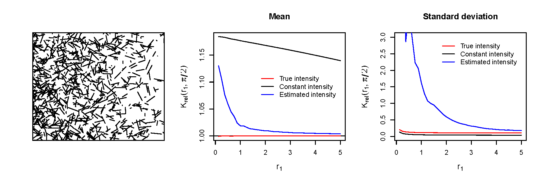
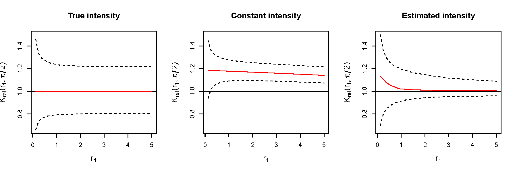
Figure 1: Top left: an example of a simulated fiber pattern. Top middle/right: mean/standard deviation of 10,000 estimates of the relative $K$-function (18) when the intensity is either known, assumed constant, or estimated linear. Lower row: mean (red curve) and 95% probability bands (dashed curves) for estimates of the relative $K$-function for the three choices of intensity functions.

For each simulation, we estimated the $K_{w}$-function by (15) using for $\rho$ either 1) the true theoretical linear expression as given in A, 2) an estimate assuming a constant intensity, or 3) the linear expression with $\beta$ estimated as described in Section 5.2.2 and with $\eta$ the true uniform density. The pointwise means, standard deviations, and 95% probability bands for the relative $K$-function

$$K_{\text{rel}}(r_{1},r_{2})=\frac{K_{w}(r_{1},r_{2})}{K_{0}(r_{1},r_{2})}$$ (18)

with $r_{2}=\tfrac{\pi}{2}$ are shown in Figure 1. We see that using the true intensity, the estimator becomes unbiased, as expected by theory. Estimating the intensity linearly results in a small positive bias, while using a constant intensity yields a larger bias of around 0.15. This bias arises because large scale variation in $\rho$ is picked up as random interaction by the $K_{w}$-function when a constant intensity is assumed.

The probability bands show that when the intensity is estimated, the resulting curves are typically closer to the mean than when the intensity is known. This phenomenon is also known from $K$-functions for point processes, see e.g. Waagepetersen and Guan (2009). Although most curves are close to the mean when the intensity is estimated linearly, a few outliers occur which is reflected in the standard deviations. This is most pronounced for small values of $r_{1}$ where estimated values of $K_{rel}(r_{1},\tfrac{\pi}{2})$ range from $-200$ to $1000$. This happens because for a few simulations, the estimated intensity comes close to zero, or even below zero, resulting in very small estimates of $\rho(z,s)$ for some $z$.

6.2 Dependent fibers

Next, we simulated 1000 realizations from a model with dependent fibers on the same window as before and using the same inhomogeneous Poisson process $Y$ for the fiber center points. To obtain dependent fibers we simulated two independent Gaussian random fields with exponential correlation function and evaluated these at the points of $Y$. For each $u$ in $Y$, the associated values of the Gaussian fields give the $x$- and $y$-coordinates of one endpoint of a centered line segment while the negation of this point forms the other endpoint resulting in a fiber symmetric around the origin. The centered fiber is next translated to have midpoint $u$. The random fields are scaled to obtain a mean fiber length of 1 as in the simulations with independent fibers. This model is described in more detail in D where it is shown that this model has $\rho$ of the form (17) with $\eta$ a uniform density and $\rho(\cdot;\beta)$ a linear model.

An example of a resulting simulated fiber pattern is shown to the left in Figure 2. Visually, it is not easy to determine exactly what is the nature of the difference between the simulations from the null model and from the model with dependent fibers. This is, however, reflected in the $K_{w}$-function. For the estimation, we replaced the unknown density function with an estimate as in option 3) for the null model in Section 6.1. The mean of the estimated relative $K$-function is shown in the right plot of Figure 2. The mean estimated $K_{rel}(r_{1},\tfrac{\pi}{2})$ does not deviate much from the value under the null model. However, the smaller the value of $r_{2}$, the larger the $K_{w}$-function becomes compared to the null model. This suggests that while the amount of fibers around a point on a given fiber is the same as under independence, fibers tend to be more aligned than under the null model. This effect is present for all $r_{1}$, but most pronounced for small values, suggesting that the correlation mainly is present on shorter scales.

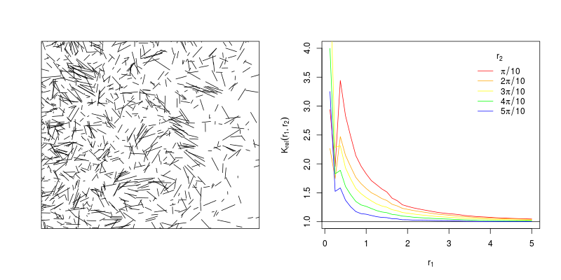
Figure 2: Left: a simulation of an inhomogeneous fiber pattern with correlated fibers. Right: the mean of the estimated relative $K$-function (18) as a function of $r_{1}$ for selected values of $r_{2}$.

7 Data example

In this section we apply our $K$-function to a 3D fiber pattern, shown in Figure 3, of steel fibers in ultra high performance fiber-reinforced concrete. The fiber pattern was extracted from a series of micro computed tomography images kindly provided by the authors of Maryamh et al. (2021). The objective in Maryamh et al. (2021) is to study the relationship between production parameters of the fiber-reinforced concrete, the spatial distribution and orientation of the steel fibers, and mechanical properties of the concrete (results of bending tests applied to concrete specimens). More specifically, the data set considered here was obtained by imaging a $160\times 40\times 40$mm block of concrete with a fiber volume percentage of 1% and with fibers of length 12.5mm and of diameter 0.3mm. Each image voxel was of sidelength 0.0906mm. Ideally, for maximal bending strength, the fibers should be aligned with the long axis of the block. Due to sedimentation, spatial inhomogeneity of the fibers is possible although the degree of inhomogeneity depends on the viscosity of the concrete used for casting the concrete block, see Maryamh et al. (2021) who considered several blocks produced with varying production parameters. Maryamh et al. (2021) studied the spatial variation in fiber density using area fraction profiles obtained from the microscope images. For the directions of fibers they obtained partial derivatives of the gray scale images and considered eigenvectors of the resulting orientation matrices. For these approaches it is not necessary to identify individual fibers. To take the analysis a step further we identified the individual fibers in order to apply our new $K_{w}$-function.

Figure 3: 3D image of a subblock of the fiber-reinforced concrete dataset.

7.1 Fiber segmentation

Since pairs of fibers are often quite close, an initial segmentation mask failed to separate all fibers. To correct this, a manual separation was performed using the ImageJ (Schneider et al., 2012) software by removing pixels that connected fibers. Each fiber was then represented by a cloud of pixel center points and the fiber cloud points were assigned fiber specific labels using a connected component algorithm implemented in the Python package SciPy (Virtanen et al., 2020). Some clouds contained very small numbers of fiber points and were discarded as artefacts of noise (in total 8% of the fiber points were discarded). To represent each fiber as a curve in space, we next obtained a least squares fit of a vector function $p(t)=(p_{x}(t),p_{y}(t),p_{z}(t))^{\mbox{\scriptsize\sf T}}$ to each fiber point cloud. Here the functions $p_{x},p_{y},p_{z}$ were chosen to be third order polynomials. As mentioned in Section 5.1.1, in practice we approximate integration along fibers with Monte Carlo integration. Specifically, we randomly generated a point process of equispaced points on each fiber. The spacing was 0.906mm corresponding to 10 image voxel side lenghts. Figure 4 shows an example of a fiber point cloud, the fitted curve, and the Monte Carlo points on the fiber curve. Tangent directions were computed at each Monte Carlo point by normalizing the derivative of $p(t)$. Since fibers are unoriented we, following Section 4, represented tangents by points on be the hemi-sphere $\mathbb{S}$ with north pole at $(0,1,0)$. Due to strong edge effects in each end of the block, we follow Maryamh et al. (2021) and discard data from the first and last (referring to the long axis) 2 cm of the block.

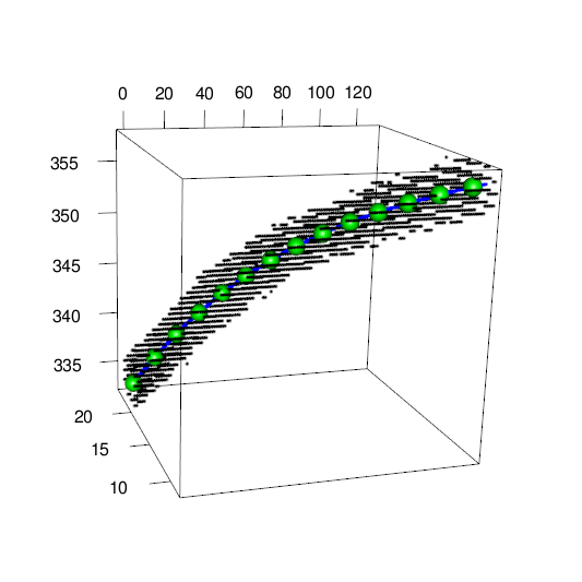
Figure 4: Example of a fiber point set, the fitted fiber curve (blue) and Monte Carlo sample points (green).

7.2 Estimation of the density function

The density function $\rho$ was fitted following the approach in Section 5.2 using the model (17) with a linear model for the space component $\rho(u;\beta)=(1,u^{\mbox{\scriptsize\sf T}})^{\mbox{\scriptsize\sf T}}\beta$, $u\in\mathbb{R}^{3}$, $\beta\in\mathbb{R}^{4}$, as suggested by C. Following Section 5.2.3, we obtained the estimate $\hat{\beta}=(1.82,0.0027,-0.0061,-0.045)^{\mbox{\scriptsize\sf T}}$. Relative to the intercept, the slopes are of moderate magnitude meaning that the volume density of the fibers is only varying moderately over space (e.g. an estimated increase in intensity of 0.32 (120 times 0.0027) across the block in the $x$-direction).

For the probability density $\eta$ for tangent directions on the hemi-sphere $\mathbb{S}$, we converted each unit tangent vector $\tau=(\tau_{1},\tau_{2},\tau_{3})$ into cylindrical coordinates $(h,\phi)=(\tau_{1},\arctan(\tau_{3}/\tau_{2}))\in[-1,1]\times[-\pi/2,\pi/2]$ (with $\arctan(0/0)=0$ and $\arctan(\pm\infty)=\pm\pi/2$.) An exploratory analysis of the height and angle cylindrical coordinates suggested to treat these as outcomes of independent random variables and assume a height distribution symmetric around zero. We hence modelled the joint density of heights and angles as a product of densities that were non-parametrically estimated by histograms, see Figure 5. Finally, the Jacobian of the mapping from the unit hemi-sphere to cylindrical coordinates is one, so the density $\eta$ is simply estimated by the estimated joint density of height and angle.

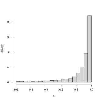
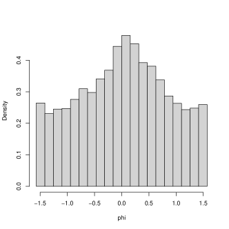
Figure 5: Left: histogram of absolute values of $x$-coordinates of unit tangent vectors. Right: angle-components (in $(y,z)$-plane) of cylindrical coordinates of unit tangent vectors.

The histograms show that the distribution of angles in the $(y,z)$ plane is roughly symmetric around 0 with moderate deviation from the uniform distribution while the distribution of heights assigns most mass at heights ($x$-coordinate of unit tangent vectors) close to one. This means that the fiber tangents are in general aligned with the $x$ direction as desired for high strength of the concrete.

7.3 The $K$-function for the concrete data

We estimated the inhomogeneous $K_{w}$-function by (15)–(16) using the intensity estimate described in Section 7.2 as weights. For comparison, we also estimated the $K_{w}$-function assuming a constant estimated intensity. The results are shown in Figure 6.

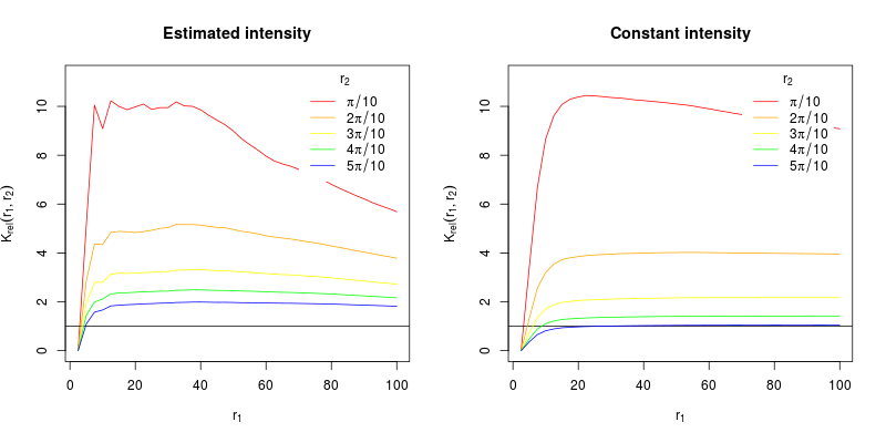
Figure 6: Relative $K$-function (18) for the concrete data set as a function of $r_{1}$ for five different values of $r_{2}$. Left: with non-constant estimated intensity. Right: with constant estimated intensity.

For the smallest angle $r_{2}=\pi/10$, the $K_{w}$-function is up to 10 times that of the null model. As $r_{2}$ increases, the $K_{w}$-function comes closer to the null model. This suggests that fiber directions tend to be locally more similar than under the null model. If we do not correct for inhomogeneity, we see the same effect. However, in this case, we cannot tell whether it is due to first-order inhomogeneity or the local alignment of fibers. For the $K_{w}$-function taking into account inhomogeneity, the deviation from the null model seems to decrease with $r_{1}$, suggesting that fiber alignment is strongest over small distances. This effect is not nearly as pronounced when constant intensity is used, possibly because the preferred fiber direction is present at all distances.

To investigate whether deviations from the null model could be due to chance, we simulated 39 fiber patterns from the null model by generating fiber midpoints from a Poisson point process with spatial intensity $\rho_{Y}$ estimated from the original dataset. To estimate $\rho_{Y}$, we assumed a linear model as in C and used (20) to obtain $\rho_{Y}(u)$ as $\eta(s)^{-1}l^{-1}\rho(u,s;\beta)$ where for $\rho$ and $\eta$ we used the estimates from Section 7.2 and for $l$ the average fiber length. For each midpoint, a fiber was sampled with replacement from the fibers in the original dataset. To compute the $K_{w}$-function, we reestimated $\rho$ by the same procedure as used for the actual dataset. The pointwise minimum and maximum values provide pointwise 95% envelopes for the relative $K$-function, see Figure 7. The relative $K$-function estimated from data is clearly outside the envelope for all the displayed values of $r_{2}=\pi/10,3\pi/10,\pi/2$, suggesting a deviation from the null model.

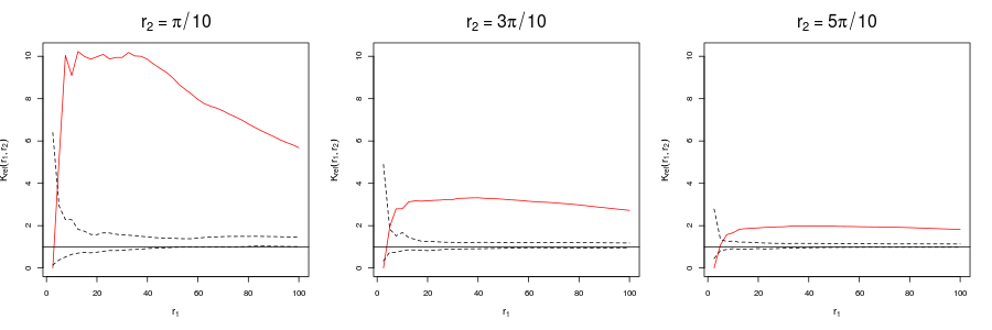
Figure 7: The relative $K$-function (18) (red curves) for three different values of $r_{2}$ with pointwise 95% envelopes (dashed curves).

8 Discussion

In this paper we developed a new $K_{w}$-function for studying random measures of the germ-grain type allowing to take geometrical features of grains into account. In particular, we considered the case of fiber patterns with associated fiber tangents. The idea of using geometrical information in second-order analyses of spatial patterns is not new (Schwandtke, 1988) but to the best of our knowledge, this idea has not before materialized in analyses of simulated and real data. In contrast to Schwandtke (1988), we moreover allow for an inhomogeneous density of the random measure. As demonstrated by our simulation studies and data example, taking into account inhomogeneity (be it spatially or with respect to the distribution of the geometrical features) may have profound implications for the interpretation of estimated $K_{w}$-functions. In contrast to Gallego et al. (2016), our assumption of distinguishable components of the random measures allow us to precisely characterize our $K_{w}$-function under the null model of independent germ-grains. This is useful as a benchmark for interpreting an estimated $K_{w}$-function.

Although we use a germ-grain/marked point process framework for our mathematical derivations, we emphasize that only knowledge of the grains/marks are required for our methodology. If the germs/points were known one might consider alternatives such as the mark-weighted $K$-function (Penttinen et al., 1992) that could be generalized to the case with an inhomogeneous density for the points. However, in addition to requiring observation of the points this would also require full observation of the marks which can be problematic due to edge effects.

Regarding estimation of first-order properties of inhomogeneous random measures, we constructed new estimating functions for fitting parametric models for the first order density $\rho$. This methodology is in fact applicable to general inhomogeneous random measures not necessarily of the germ-grain type considered in this paper.

A practical issue in relation to applying our $K_{w}$-function is that identifying the individual grains (e.g. fibers) from image data may not be straightforward. For our data, this required a substantual amount of manual work and there is certainly scope for research in improved image processing algorithms. A theoretical topic for future research is to widen the catalogue of specific models for which the reweighted second-order measure $\alpha_{w}^{(2)}$ is known to be stationary.
Acknowledgments Hans J. T. Stephensen was supported by QIM - Center for Quantification of Imaging Data from MAX IV. The concrete fiber data and Figure 3 was kindly provided by Claudia Redenbach, Technische Universität Kaiserslautern. The concrete fiber data is a result of joint work by Kasem Maryamh (sample), Technische Universität Kaiserslautern, Franz Schreiber (imaging), Fraunhofer ITWM, and Konstantin Hauch (binarization), Technische Universität Kaiserslautern.

Appendix A A simple fiber model

A random line segment $\Gamma$ generates the random measure

$$m(A\times S)=\int_{\Gamma}\mathds{1}[x\in A,\tau(x)\in S]\lambda(\mathrm{d}x),A\subseteq\mathbb{R}^{d},S\subseteq\mathbb{S}^{d-1}.$$

If $\Gamma$ is centered at the origin, of random length $L$, and of randomly distributed orientation $\Theta\in\mathbb{S}^{d-1}$, then

$$m(A\times S)=\int_{-L/2}^{L/2}\mathds{1}[r\Theta\in A,\Theta\in S]\mathrm{d}r.$$

Assuming moreover that $L$ and $\Theta$ are independent and $\Theta$ has a density $\eta$ with respect to $\nu$, we obtain

$${\mathbb{E}}m(A\times S)=\int_{\mathbb{S}^{d-1}}\mathbb{E}\int_{-L/2}^{L/2}\eta(\theta)\mathds{1}[r\theta\in A,\theta\in S]\mathrm{d}r\nu(\mathrm{d}\theta).$$

Consider a fiber process where, given the underlying point process $Y$, the marks are line segments identically distributed as $\Gamma$ translated to have midpoints in $Y$. Then,

$$\mu(A\times S)= \int_{\mathbb{R}^{d}}\rho_{Y}(u){\mathbb{E}}[m((A-u)\times S)]\mathrm{d}u$$

$$= \int_{\mathbb{S}^{d-1}}\mathds{1}[\theta\in S]\int_{\mathbb{R}^{d}}\rho_{Y}(u)\mathbb{E}\int_{-L/2}^{L/2}\eta(\theta)\mathds{1}[r\theta+u\in A]\mathrm{d}r\mathrm{d}u\nu(\mathrm{d}\theta)$$

$$= \int_{\mathbb{S}^{d-1}}\int_{\mathbb{R}^{d}}\mathds{1}[z\in A,\theta\in S]\mathbb{E}\int_{-L/2}^{L/2}\eta(\theta)\rho_{Y}(z-r\theta)\mathrm{d}r\mathrm{d}z\nu(\mathrm{d}\theta).$$

Hence $\mu$ has density

$$\rho(z,s)=\eta(s)\mathbb{E}\int_{-L/2}^{L/2}\rho_{Y}(z-rs)\mathrm{d}r.$$

Suppose $\rho_{Y}$ is given in terms of a linear model $\rho_{Y}(u)=\beta_{0}+\beta^{\mbox{\scriptsize\sf T}}u$. Then

$$\rho(z,s)=\eta(s)\mathbb{E}\int_{-L/2}^{L/2}[\beta_{0}+\beta^{\mbox{\scriptsize\sf T}}(z-rs)]\mathrm{d}r=\eta(s)l(\beta_{0}+\beta^{\mbox{\scriptsize\sf T}}z),$$

where $l=\mathbb{E}L$.

Appendix B An alternative choice of weights

For the weights $w(u,x,s)=\xi_{u}(x,s)\rho_{Y}(u)$ suggested in Remark 3.5 assume that $\xi_{u}(\cdot,s)$ has a bounded support $u+C$ where $C$ does not depend on $u$ or $s$. Then $\mu_{w}(A\times S)=|A|\nu(S)|C|$. Assuming that $\xi_{u,u^{\prime}}$ exists, define

$$g_{u,u^{\prime}}(x,s,y,t)=\frac{\xi_{u,u^{\prime}}(x,s,y,t)}{\xi_{u}(x,s)\xi_{u^{\prime}}(y,t)}\mathds{1}[x-u,y-u^{\prime}\in C].$$

By (8) and (9),

$${\mathbb{E}}\sum_{(u,m),(u^{\prime},m^{\prime})\in X}^{\neq}\int_{(\mathbb{R}^{d}\times\mathbb{S})^{2}}f(x,s,y,t)m(\mathrm{d}x\times\mathrm{d}s)m^{\prime}(\mathrm{d}y\times\mathrm{d}t)$$

$$= \int_{(\mathbb{R}^{d}\times\mathbb{S})^{2}}f(x,s,y,t)\int_{\mathbb{R}^{d}\times\mathbb{R}^{d}}\rho_{Y}(u)\rho_{Y}(u^{\prime})g_{Y}(u,u^{\prime})\xi_{u,u^{\prime}}((x,s),(y,t))$$

$$\mathrm{d}u\mathrm{d}u^{\prime}\mathrm{d}x\mathrm{d}y\nu(\mathrm{d}s)\nu(\mathrm{d}t).$$

We thus have the following expression for $K_{w}$:

$$K_{w}(r_{1},r_{2};W)$$

$$= \frac{1}{|W|}\int_{\mathbb{R}^{d}\times\mathbb{R}^{d}}\int_{(C+u)\times(C+u^{\prime})\times\mathbb{S}^{2}}\mathds{1}[x\in W]\mathds{1}[\|x-y\|\leq r_{1},d_{\mathbb{S}}(s,t)\leq r_{2}]$$

$$\cdot g_{u,u^{\prime}}(x,s,y,t)g_{Y}(u,u^{\prime})\mathrm{d}x\mathrm{d}y\nu(\mathrm{d}s)\nu(\mathrm{d}t)\mathrm{d}u\mathrm{d}u^{\prime}.$$

Stationarity of $\alpha_{w}^{(2)}$ is obtained if for all $h\in\mathbb{R}^{d}$

$$g_{Y}(u,u^{\prime})=g_{Y}(u+h,u^{\prime}+h)\,\,\text{and}\,\,g_{u,u^{\prime}}(x,s,y,t)=g_{u+h,u^{\prime}+h}(x+h,s,y+h,t).$$ (19)

In this case,

$$K_{w}(r_{1},r_{2};W)= \int_{\mathbb{R}^{d}\times(C\times\mathbb{S})^{2}}\mathds{1}[\|x-y-l\|\leq r_{1},d_{\mathbb{S}}(s,t)\leq r_{2}]$$

$$\cdot g_{0,l}(x,s,y+l,t)g_{Y}(0,l)\mathrm{d}x\mathrm{d}y\nu(\mathrm{d}s)\nu(\mathrm{d}t)\mathrm{d}l.$$

The first condition in (19) requires that $Y$ is second-order intensity reweighted stationary which is a fairly weak requirement, see Baddeley et al. (2000). The second requirement is for instance satisfied if $\xi_{u}(x,s)=\xi(x-u,s)$ for a common $\xi$ not depending on $u$ and if, similarly, $\mathbb{E}_{u,u^{\prime}}m(\cdot)m^{\prime}(\cdot)$ is translation invariant, $\mathbb{E}_{u,u^{\prime}}m(\cdot)m^{\prime}(\cdot)=\mathbb{E}_{u+h,u^{\prime}+h}m(\cdot+h)m^{\prime}(\cdot+h)$, $h\in\mathbb{R}^{d}$. This is for instance the case for the model with dependent fibers used for simulation in Section 6.

Under the null model, $g_{Y}=1$ and $\xi_{u,u^{\prime}}=\xi_{u}\xi_{u^{\prime}}$. Then $g_{0,l}(x,s,y,t)g_{Y}(0,l)=\mathds{1}[x,y\in C]$ and

$$K_{w}(r_{1},r_{2})=K_{0}(r_{1},r_{2})|C|^{2},$$

where $K_{0}$ is as in (11). In practice $|C|$ is not known. Given an estimate $\hat{K}_{w}$ we might consider the ratio $\hat{K}_{w}(r_{1},r_{2})/K_{0}(r_{1},r_{2})$ which should be close to a constant over $r_{1}$ and $r_{2}$ under the null model.

For more general models, if $g_{u,u^{\prime}}(x,s,y,t)\leq(\geq)1$ and $g_{Y}(u,u^{\prime})\leq(\geq)1$ for all $u,u^{\prime}\in\mathbb{R}^{d}$ and all $(x,s,y,t)\in(C\times\mathbb{R}^{d})^{2}$, then $K_{w}(r_{1},r_{2})\leq(\geq)K_{0}(r_{1},r_{2})|C|^{2}$ for all $r_{1},r_{2}$.

Appendix C A model with reflection invariant mean mark density

Suppose that $\xi_{u}(x,s)=\xi(x-u,s)$ where $\xi$ satisfies $\xi(x,s)=\xi(-x,s)$. This is for example satisfied is $\xi(\cdot,s)$ is a density with elliptical contours centered at the origin. With

$$\rho_{Y}(u)=\beta_{0}+\beta^{\mbox{\scriptsize\sf T}}u$$

and defining

$$\tilde{\xi}(s)=\int_{\mathbb{R}^{d}}\xi(x,s)\mathrm{d}x,$$

we obtain

$$\rho(z,s)= \frac{1}{2}\int_{\mathbb{R}^{d}}(\xi(x,s)+\xi(-x,s))(\beta_{0}+\beta^{\mbox{\scriptsize\sf T}}[z-x])\mathrm{d}x$$

$$= (\beta_{0}+\beta^{\mbox{\scriptsize\sf T}}z)\int_{\mathbb{R}^{d}}\xi(x,s)\mathrm{d}x+\frac{1}{2}\int_{\mathbb{R}^{d}}\xi(x,s)\beta^{\mbox{\scriptsize\sf T}}[-x+x]\mathrm{d}x$$

$$= (\beta_{0}+\beta^{\mbox{\scriptsize\sf T}}z)\tilde{\xi}(s).$$

Defining

$$l=\int_{\mathbb{S}^{d-1}}\tilde{\xi}(s)\nu(\mathrm{d}s)$$

and the probability density

$$\eta(s)=\tilde{\xi}(s)/l,$$

we obtain

$$\rho(z,s)=\eta(s)l\rho_{Y}(z).$$ (20)

Suppose now that $\rho_{Y}(z)$ is non-linear in $z$, that $\xi(\cdot,\cdot)$ has bounded support $C$ with respect to the first argument, and that $\rho_{Y}(\cdot)$ is well approximated by its tangent plane on $C+z$. The convolution

$$\rho(z,s)=\int_{\mathbb{R}^{d}}\xi(z-u,s)\rho_{Y}(u)\mathrm{d}u$$

only involves $\rho_{Y}(u)$ for $u\in C+z$. Hence we obtain

$$\rho(z,s)\approx\eta(s)l\rho_{Y}(z)$$

following the arguments leading to (20).

Appendix D A model with dependent fibers

We now describe the model used for simulation of dependent fibers in Section 6. We again choose $Y$ as a Poisson process and generate independent stationary zero-mean Gaussian fields $X_{1},\ldots,X_{d}$ such that ${\mathbb{V}\mathrm{ar}}X_{i}(u)={\mathbb{V}\mathrm{ar}}X_{j}(u)$, $u\in\mathbb{R}^{d}$, $i,j=1,\ldots,d$. For a location $u$, we further let $X(u)=(X_{1}(u),\ldots,X_{d}(u))$, $L_{u}=\|X(u)\|$ and $T_{u}=X(u)/L_{u}$. Then $T_{u}$ has uniform density $\eta$ on $\mathbb{S}^{d-1}$ and is independent of $L_{u}$. Each point $u\in Y$ is marked by the line segment $\Gamma_{u}$ from $-X(u)$ to $X(u)$ translated by $u$. The fiber measure $m$ associated to $\Gamma_{u}$ is

$$m(A\times S)=\int_{\Gamma_{u}}\mathds{1}[z\in A,T_{u}\in S]\lambda(\mathrm{d}z)=L_{u}\int_{-1}^{1}\mathds{1}[u+tT_{u}L_{u}\in A,T_{u}\in S]\mathrm{d}t.$$

Since the distribution of $\Gamma_{u}$ is independent of $u$, we get from A that $\mu$ has density

$$\rho(z,s)=\eta(s)\int_{-L_{u}}^{L_{u}}{\mathbb{E}}[\rho_{Y}(z-rs)]\mathrm{d}r$$

and if $\rho_{Y}$ is linear $\rho_{Y}(u)=\beta_{0}+\beta^{\mbox{\scriptsize\sf T}}u,$ then

$$\rho(z,s)=\eta(s)l(\beta_{0}+\beta^{\mbox{\scriptsize\sf T}}z)$$

with $l=2{\mathbb{E}}L_{u}$.

References

- Baddeley et al. (2015) Baddeley, A., Rubak, E. and Turner, R. (2015) Spatial Point Patterns: Methodology and Applications with R. London: Chapman and Hall/CRC Press.
- Baddeley et al. (2000) Baddeley, A. J., Møller, J. and Waagepetersen, R. (2000) Non- and semi-parametric estimation of interaction in inhomogeneous point patterns. Statistica Neerlandica, 54, 329–350.
- Chiu et al. (2013) Chiu, S., Stoyan, D., Kendall, W. and Mecke, J. (2013) Stochastic Geometry and Its Applications. Wiley Series in Probability and Statistics. Wiley.
- Gallego et al. (2016) Gallego, M. A., Ibáñez, M. V. V. and Simó, A. (2016) Inhomogeneous -function for germ–grain models. Spatial Statistics, 18, 489 – 504.
- Hansen et al. (2021) Hansen, P. E. H., Waagepetersen, R., Svane, A. M., Sporring, J., Stephensen, H. J. T., Hasselholt, S. and Sommer, S. (2021) Generalizations of Ripley’s -function with application to space curves. In Proceedings of the GSI’21.
- Jensen et al. (1990) Jensen, E., Kiêu, K. and Gundersen, H. (1990) On the stereological estimation of reduced moment measures. Ann Inst Stat Math, 42, 445–461.
- Van Lieshout (2018) Van Lieshout, M. N. M. (2018) Nonparametric indices of dependence between components for inhomogeneous multivariate random measures and marked sets. Scandinavian Journal of Statistics, 45, 985–1015.
- Maryamh et al. (2021) Maryamh, K., Hauch, K., Redenbach, C. and Schnell, J. (2021) Influence of production parameters on the fiber geometry and the mechanical behavior of ultra high performance fiber-reinforced concrete. Structural Concrete, 22, 361–375.
- Møller and Waagepetersen (2017) Møller, J. and Waagepetersen, R. (2017) Some recent developments in statistics for spatial point processes. Annual Review of Statistics and its Applications, 4, 317–342.
- Møller and Waagepetersen (2004) Møller, J. and Waagepetersen, R. P. (2004) Statistical Inference and Simulation for Spatial Point Processes. Boca Raton: CRC Press.
- Møller and Waagepetersen (2007) — (2007) Modern statistics for spatial point processes. Scandinavian Journal of Statistics, 34, 643–684.
- Penttinen et al. (1992) Penttinen, A., Stoyan, D. and Henttonen, H. M. (1992) Marked point processes in forest statistics. Forest Science, 38, 806–824.
- Ripley (1976) Ripley, B. D. (1976) The second-order analysis of stationary point processes. Journal of Applied Probability, 13, 255–266.
- Schneider et al. (2012) Schneider, C. A., Rasband, W. S. and Eliceiri, K. W. (2012) NIH image to ImageJ: 25 years of image analysis. Nature Methods, 9, 671–675.
- Schwandtke (1988) Schwandtke, A. (1988) Second-order quantities for stationary weighted fibre processes. Mathematische Nachrichten, 139, 321–334.
- Shaw et al. (2020) Shaw, T., Møller, J. and Waagepetersen, R. (2020) Globally intensity-reweighted estimators for - and pair correlation functions. Australian and New Zealand Journal of Statistics, 63, 93–118.
- Stoyan and Ohser (1982) Stoyan, D. and Ohser, J. (1982) Correlations between planar random structures with an ecological application. Biometrical Journal, 24, 631–647.
- Virtanen et al. (2020) Virtanen, P., Gommers, R., Oliphant, T. E., Haberland, M., Reddy, T., Cournapeau, D., Burovski, E., Peterson, P., Weckesser, W., Bright, J., van der Walt, S. J., Brett, M., Wilson, J., Millman, K. J., Mayorov, N., Nelson, A. R. J., Jones, E., Kern, R., Larson, E., Carey, C. J., Polat, İ., Feng, Y., Moore, E. W., VanderPlas, J., Laxalde, D., Perktold, J., Cimrman, R., Henriksen, I., Quintero, E. A., Harris, C. R., Archibald, A. M., Ribeiro, A. H., Pedregosa, F., van Mulbregt, P. and SciPy 1.0 Contributors (2020) SciPy 1.0: Fundamental Algorithms for Scientific Computing in Python. Nature Methods, 17, 261–272.
- Waagepetersen (2007) Waagepetersen, R. (2007) An estimating function approach to inference for inhomogeneous Neyman-Scott processes. Biometrics, 63, 252–258.
- Waagepetersen and Guan (2009) Waagepetersen, R. and Guan, Y. (2009) Two-step estimation for inhomogeneous spatial point processes. Journal of the Royal Statistical Society, Series B, 71, 685–702.