The Cut-and-Play Algorithm: Computing Nash Equilibria via Outer Approximations

Abstract

We introduce the Cut-and-Play, an efficient algorithm for computing equilibria in simultaneous non-cooperative games where players solve nonconvex and possibly unbounded optimization problems. Our algorithm exploits an intrinsic relationship between the equilibria of the original nonconvex game and the ones of a convexified counterpart. In practice, Cut-and-Play formulates a series of convex approximations of the original game and refines them with techniques from integer programming, for instance, cutting planes and branching operations. We test our algorithm on two families of challenging nonconvex games involving discrete decisions and bilevel programs, and we empirically demonstrate that it efficiently computes equilibria and outperforms existing game-specific algorithms.

1 Introduction

Decision-making is hardly an individual task; instead, it often involves the mutual interaction of several self-driven decision-markers, or players, and their heterogeneous preferences. The most natural framework to model each player’s decision problem is often an optimization problem whose solutions, or strategies, provide prescriptive recommendations on the best course of action. However, in contrast with optimization, the solution to the game involves the concept of stability, i.e., a condition ensuring that the players are playing mutually-optimal strategies. In two seminal papers, Nash [43, 42] formalized a solution concept for finite non-cooperative games, namely, the concept of Nash equilibrium. Nash equilibria are stable solutions, as no rational and self-driven decision-maker can unilaterally and profitably defect them.

Historically, convexity played a central role in shedding light on the existence and computation of Nash equilibria (e.g., see Facchinei and Pang [28], Daskalakis [19] and the references therein). Indeed, von Neumann [58] proved that 2-player zero-sum games always admit a Nash equilibrium if the players’ cost (payoff) functions are convex (concave) in their strategies, and the conditions yielding Nash equilibria are essentially equivalent to linear-programming duality [18]. However, the plausibility of the Nash equilibrium also stems from the availability of algorithms to compute it. As Roth [51] argued in his claim “economists as engineers”, computing Nash equilibria plays a central role in designing markets and deriving pragmatic insights. For instance, from the perspective of an external regulator, Nash equilibria are invaluable tools for understanding how to design and intervene in markets to balance the agents’ individual interests with societal goals. However, markets and their mathematical models rarely satisfy well-structured convexity assumptions: nonconvexities often model complex operational requirements and are vital to accurately represent reality and extract valid conclusions. Although there is a wealth of methodologies to compute Nash equilibria for finite games described, for example, in normal-form and, generally, for games satisfying convexity assumptions, little is known about the computation of equilibria in nonconvex settings [19]. This gap represents the core motivation of this work.

This paper presents an efficient method for computing equilibria in non-cooperative games where players solve nonconvex optimization problems. The nonconvexities may stem from, for instance, integer variables modeling indivisible quantities and logical conditions, bilevel constraints rendering hierarchical relationships among decision-makers, and from several other nonconvexities naturally associated with physical phenomena, e.g., water distribution and signal processing [47, 31]. Because of their extreme practical interest, several methodologies in optimization have made certain nonconvexities tractable, at least from a computational perspective. Although some recent papers focused on games with specific types of nonconvexities (e.g., integer variables [39, 52, 17, 55, 31, 8, 23, 10] and bilevel [46, 9, 56, 35]), to date, there is no general-purpose algorithm to compute Nash equilibria in games where different nonconvexities arise.

Our Contributions.

This paper presents an efficient algorithm to compute equilibria for a large class of games where players decide by solving parametrized optimization problems with nonconvex feasible regions. Specifically, we assume each player optimizes a separable function in its variables, i.e., a function expressed as a weighted sum-of-products function in the player’s variables [27, 26, 57]. We summarize our contributions as follows:

1. We prove that when the player’s objective functions (i.e., payoffs) are separable, the game admits an equivalent convex representation, even if the players’ feasible sets are inherently nonconvex. We present this equivalence in terms of a novel correspondence between the Nash equilibria of the original game and those of a convexified game where each player’s feasible set gets replaced by its (closed) convex hull.

2. We introduce Cut-and-Play (CnP), a cutting plane algorithm to compute Nash equilibria for a large family of simultaneous and non-cooperative $n$-player nonconvex games. In essence, this algorithm exploits a sequence of convexifications of the original nonconvex game and involves a well-crafted mix of Mixed-Integer Programming (MIP) techniques; for instance, it blends concepts such as relaxation (approximation), valid inequalities, disjunctive programming, and branching along with complementarity problems. The algorithm finds an exact Nash equilibrium or proves its non-existence, and it resembles the iterative refinement of approximations (or, more precisely, relaxations) that a branch-and-cut algorithm would perform on an optimization problem. To our knowledge, this is the first approach exploiting outer approximations to compute Nash equilibria.

3. Our algorithm is general and problem-agnostic as it supports several types of nonconvexities. Compared to the previous works, CnP possesses several distinctive elements. Specifically, our algorithm does not: (a.) require that the players’ optimization problems are convex or continuous (b.) compute only pure (i.e., deterministic) equilibria (c.) change with respect to the type of nonconvexities, or (d.) rely on alternative or weaker concepts of equilibria . Finally, our algorithm does not require the players to have a finite number of strategies, e.g., as in normal-form games; on the contrary, it supports uncountable strategy sets and can also certify the non-existence of equilibria.

4. We present an extensive set of computational results on two important families of challenging nonconvex games: Integer Programming Games (IPGs) and Nash games among Stackelberg Players (NASPs), i.e., a class of simultaneous games among players solving integer and bilevel programs, respectively. In both cases, our algorithm outperforms the baselines in terms of computing times and solution quality.

Outline.

We structure the paper as follows. Section 2 provides a literature review, and Section 3 formalizes the background definitions and our notation. Sections 4 and 5 present the principles behind our approach and introduce the CnP algorithm and its practical implementation. Section 6 details how to customize CnP when some of the game’s structure is known, and it showcases a comprehensive set of computational results. Finally, we present our conclusions in Section 7.

2 Literature Review

Nash [43, 42] formalized the concept of stability in non-cooperative simultaneous games through the Nash equilibrium. We distinguish between two types of equilibria: Pure Nash Equilibria (PNEs), where players employ deterministic strategies, and Mixed Nash Equilibria (MNEs), where players randomize over their strategies. If the game is finite, i.e., there are finitely many players and strategies, Nash proved that an MNE always exists. Glicksberg [32] extended the result, proving that an MNE always exists when players have continuous payoff functions and compact strategy sets. Although MNEs are guaranteed to exist under some assumptions, an equilibrium may not exist in the general case. For instance, in IPGs and other nonconvex games, deciding if an MNE exists is $\Sigma^{p}_{2}$-complete [6, 8, 9], i.e., it is at the second level of the polynomial hierarchy of complexity [60]. Besides existence, computing equilibria or certifying their non-existence pose significant algorithmic challenges [20].

Equilibria in Finite Games.

Most algorithmic approaches for computing Nash equilibria deal with finite games represented in normal form, i.e., through payoff matrices describing the outcome under any combination of the players’ strategies. Besides duality for 2-player zero-sum games [58], the first algorithm for computing equilibria in $2$-player normal-form games is the Lemke-Howson [41]. Although Wilson [59] and Rosenmüller [50] extended the Lemke-Howson to $n$-player normal-form games, their methods often require the solution of a series of nonlinear systems. More recently, Sandholm et al. [54] and Porter et al. [49] proposed two algorithms for 2-player normal-form games exploiting the idea of support enumeration, i.e., the idea of computing an equilibrium by guessing the strategies played with strictly positive probability in an equilibrium. Porter et al. [49] solve a system of inequalities (nonlinear for more than $2$ players) to determine whether a given support (i.e., a subset of pure strategies for each player) leads to an equilibrium. Sandholm et al. [54] avoid an (explicit) support enumeration by modeling the same idea via a MIP problem. In contrast to the above literature, we focus on a broader class of games (containing 2-player normal-form games), where the number of pure strategies can be exponential, perhaps uncountable, in the input size of the game. Therefore, the above approaches are impractical, as an explicit enumeration of pure strategies would be inefficient.

Equilibria in Continuous Games.

If each player’s optimization problem is convex and continuous in its strategies, equilibrium programming methods can often determine a Nash equilibrium by: 1. reformulating the game as a complementarity or variational inequality problem [15], and 2. employing globally-convergent Jacobi or Gauss-Seidel algorithms [28]. On the one hand, these reformulations require restrictive convexity assumptions on the players’ optimization problems and may not otherwise guarantee convergence. Besides a few exceptions (e.g., Sagratella [52]), to date, the majority of equilibrium programming methods require convexity and, otherwise, develop weaker concepts of equilibrium, for instance, quasi Nash equilibria [47, 44]. On the other hand, they generally have the advantage of being extremely scalable and efficient under convexity. CnP exploits this efficiency by solving, at each iteration, a convexified game via a complementarity problem.

Equilibria and Integer Nonconvexities.

In the particular case of integer nonconvexities, Köppe et al. [39] introduced the taxonomy of IPGs, i.e., non-cooperative games where each player solves a parametrized integer program. IPGs generalize any finite game and implicitly describe the set of strategies via constraints, as opposed to the explicit description of, for instance, normal-form games. Arguably, IPGs represent the most prominent emerging family of nonconvex games and have several application domains, for instance, cyber-security [25], kidney exchange markets [5], transportation [53], and facility location [7, 40, 16, 17]. Several authors recently developed algorithms to compute IPGs’ Nash equilibria with a variety of different assumptions [52, 55, 8, 17, 23, 34]; we refer the reader to the tutorial Carvalho et al. [10] and the references therein for a detailed survey. Compared to IPGs algorithms, CnP handles other nonconvexities besides integer ones. Furthermore, as opposed to the majority of the algorithms besides the Sample Generation Method (SGM) of [8] for IPGs, CnP considers the more general concept of MNE, instead of PNE.

3 The Problem and Our Assumptions

3.1 Separable-Payoff Games

As a standard game-theory notation, let the operator $(\cdot{})^{-i}$ represent the elements of $(\cdot{})$ but the $i$-th element. We focus on nonconvex Separable-Payoff Games (SPGs), a large family of games where each player’s objective takes a sum-of-products form [27, 26, 57], as formalized in Definition 1.

Definition 1 (Separable-Payoff Game).

An SPG $G=(P^{1},\dots,P^{n})$ is a non-cooperative, complete-information, and simultaneous game among $n$ players with each player $i=1,2,\dots,n$ solving the optimization problem

$$\min_{x^{i}}\{f^{i}(x^{i};x^{-i}):=(c^{i})^{\top}x^{i}+\sum_{j=1}^{m_{i}}g^{i}_{j}(x^{-i})x^{i}_{j}\quad\text{ subject to }\quad x^{i}\in\mathcal{X}^{i}\subseteq\mathbb{R}^{m_{i}}\}, P^{i}$$ ()

where, for each player $i$, $\mathcal{X}^{i}\neq\emptyset$ is the set of player $i$’s strategies, $c^{i}$ is a real-valued vector, and $g^{i}_{j}(x^{-i})$ is of the form $g^{i}_{j}(x^{-i})=\prod_{\begin{subarray}{c}k=1,k\neq i\end{subarray}}^{n}h^{i}_{jk}(x^{k})$ with $h^{i}_{jk}$ being an affine function. An SPG is polyhedrally representable if, for each $i$, $\operatorname{cl}\operatorname{conv}(\mathcal{X}^{i})$ (i.e., the closure of the convex hull of $\mathcal{X}^{i}$) is a polyhedron.

From Definition 1, the optimization problem $P^{i}$ of player $i$ is parametrized in its opponent choices $x^{-i}$. When we say the game has complete information, we mean that all the parameters of the players’ optimization problems (i.e., $c^{i},g^{i}_{j}$, and $\mathcal{X}^{i}$ for each $i$ and $j=1,\dots,m_{i}$) are shared knowledge. By simultaneous, we mean that the players decide simultaneously without knowing their opponents’ choices. For each player $i$, we call $x^{i}\in\mathcal{X}^{i}$ a pure strategy, $\mathcal{X}^{i}$ the feasible set (or set of strategies), and $f^{i}(x^{i};x^{-i})$ the payoff of $i$ under $x=(x^{i},x^{-i})$.

Remark 1 (Linear Form).

Without loss of generality, in Definition 1, we present SPGs in a linear form, i.e., we let $c^{i}$ be a vector and $h^{i}_{jk}(x^{k})$ be affine functions. If the objective of player $i$ is instead $s_{i}(x^{i})+\sum_{j=1}^{m_{i}}g^{i}_{j}(x^{-i})q^{i}_{j}(x^{i})$, where $s^{i}$ and $q^{i}_{j}$-s are nonlinear functions, and $g^{i}_{j}(x^{-i})$ is the product of nonlinear functions $h^{i}_{jk}(x^{k})$ for $k=1,2,\dots,(i-1),(i+1),\dots,n$, we can always reformulate the game so that each payoff has the form of Definition 1. To this end, we can introduce 1. the auxiliary variables $\gamma^{i}$, $\psi^{i}_{j}$ and the constraints $\gamma^{i}=s^{i}(x^{i})$, $\psi^{i}_{j}=q^{i}_{j}(x^{i})$ in $P^{i}$, and 2. for each $j=1,\dots,m_{i}$ and $k$, an auxiliary variable $\delta^{i}_{jk}$ and a constraint $\delta^{i}_{jk}=h^{i}_{jk}(x^{k})$ in $P^{k}$. Thus, the payoff of player $i$ becomes $\gamma^{i}+\sum_{j-1}^{m_{i}}\left(\prod_{k\neq i}\delta^{i}_{jk}\right)x^{i}_{j}$, which is in linear form. Furthermore, if $s^{i}(x^{i})$ is convex, we can write the convex constraint $\gamma^{i}\geq s^{i}(x^{i})$ instead of the equality version. Finally, we remark that SPGs can represent broad classes of games, for instance, any normal-form game and separable game (which, in addition to separable payoffs, requires $\mathcal{X}^{i}$ to be a compact set).

Mixed Strategies and Equilibria.

For each player $i$, $\sigma^{i}$ is a mixed strategy, or simply a strategy, if it is a probability distribution over the pure strategies $\mathcal{X}^{i}$. Let $\Delta^{i}$ be the space of atomic probability distributions over $\mathcal{X}^{i}$ such that $\sigma^{i}\in\Delta^{i}$. Let $\operatorname{supp}(\sigma^{i}):=\{x^{i}\in\mathcal{X}^{i}:\sigma^{i}(x^{i})>0\}$ be the support of the strategy $\sigma^{i}$, where $\sigma^{i}(x^{i})$ is the probability of playing $x^{i}$ in $\sigma^{i}$. If a mixed strategy $\sigma^{i}$ has singleton support, i.e., $|\operatorname{supp}(\sigma^{i})|=1$, then it is also a pure strategy. We denote $\sigma^{-i}\in\prod_{j=1,i\neq j}^{n}\Delta^{j}$ the other players’ strategies, a probability distribution over the strategies of $i$’s opponents. If $\mathcal{X}^{i}$ is a compact set, any mixed-strategy $\sigma^{i}$ of an SPG has an equivalent finitely supported mixed-strategy $\widehat{\sigma}^{i}$ [57]; here, the equivalence means that each player $i$’s expected payoff under $\sigma^{i}$ is equal to the one under $\widehat{\sigma}^{i}$. This result extends to SPGs, with $\mathcal{X}^{i}$ possibly non-compact, as long as the support of $\sigma^{i}$ is a compact set; this is why we define $\Delta^{i}$ via atomic distributions over $\mathcal{X}^{i}$. The expected payoff for $i$ for the mixed strategy profile $\sigma=(\sigma^{1},\dots,\sigma^{n})$ is

$$\mathbb{E}_{\begin{subarray}{c}X\sim\sigma\end{subarray}}\left[f^{i}(X^{i};X^{-i})\right]\quad= \quad f^{i}(\sigma^{i};\sigma^{-i})\quad=$$

$$\quad= \sum_{x^{i}\in\operatorname{supp}(\sigma^{i})}(c^{i})^{\top}x^{i}\sigma^{i}(x^{i})+\sum_{x\in\operatorname{supp}(\sigma)}\left(\sigma^{i}(x^{i})\sum_{j=1}^{m_{i}}g^{i}_{j}(\sigma^{-i}(x^{-i})x^{-i})x^{i}_{j}\right).$$ (1)

For simplicity, we will refer to Section 3.1 as $f^{i}(\sigma^{i};\sigma^{-i})$. A strategy $\overline{\sigma}^{i}$ is a best response for player $i$ given its opponents’ strategies $\overline{\sigma}^{-i}$ if $f^{i}(\overline{\sigma}^{i};\overline{\sigma}^{-i})\leq f^{i}(\widehat{\sigma}^{i};\overline{\sigma}^{-i})$ for any possible deviation $\widehat{\sigma}^{i}\in\Delta^{i}$; in practice, we can restrict the search of deviations $\widehat{\sigma}^{i}$ to pure strategies. A strategy profile $\overline{\sigma}=(\overline{\sigma}^{1},\dots,\overline{\sigma}^{n})$ is an MNE if, for each player $i$ and strategy $\widehat{\sigma}^{i}\in\Delta^{i}$, then $f^{i}(\overline{\sigma}^{i};\overline{\sigma}^{-i})\leq f^{i}(\widehat{\sigma}^{i};\overline{\sigma}^{-i})$.

3.2 Polyhedral Representability

Our algorithmic framework hinges on the assumption of polyhedral representability. In other words, for any player $i$, we assume that $\operatorname{cl}\operatorname{conv}(\mathcal{X}^{i})$, i.e., the closure of the convex hull of the set of feasible strategies $\mathcal{X}^{i}$, is a polyhedron. For instance, $\mathcal{X}^{i}$ could be a set of linear inequalities and integrality requirements or the feasible set of a linear bilevel program. Whenever $\operatorname{cl}\operatorname{conv}(\mathcal{X}^{i})$ is polyhedral for every player $i$, we prove that our algorithm terminates with either an MNE or a proof of its non-existence. Naturally, if $\mathcal{X}^{i}$ is either a polyhedron or a union of polyhedra, then $\operatorname{cl}\operatorname{conv}(\mathcal{X}^{i})$ is polyhedral; otherwise, as we illustrate in Examples 1, 2 and 3, the game can still be polyhedrally representable even if $\mathcal{X}^{i}$ is not polyhedral.

Example 1 (Conic Player).

Consider a player $i$, and let $\mathcal{X}^{i}=\{x^{i}\in\mathbb{R}^{3}:(x^{i}_{1})^{2}+(x^{i}_{2})^{2}\geq x^{i}_{3},-x^{i}_{3}\leq x^{i}_{1},x^{i}_{2}\leq x^{i}_{1},x^{i}_{3}\geq 0\}$. The closure of the convex-hull of $\mathcal{X}^{i}$ is the polyhedron $\operatorname{cl}\operatorname{conv}(\mathcal{X}^{i})=\{-x^{i}_{3}\leq x^{i}_{1},x^{i}_{2}\leq x^{i}_{3},x^{i}_{3}\geq 0\}$.

Example 2 (Integer-Linear Bilevel Player).

Consider a player $i$, and let

$$\mathcal{X}^{i}=\big{\{}A^{i}x^{i}+B^{i}y^{i}\geq b^{i},x^{i}\in\mathbb{Z}^{m_{i}},y^{i}\in\arg\min_{y^{i}}\{(d^{i})^{\top}y^{i}:D^{i}y^{i}+E^{i}x^{i}\geq o^{i},y^{i}\geq 0\}\big{\}},$$

where $A^{i}$, $B^{i}$, $D^{i}$, $E^{i}$, and $b^{i}$, $o^{i}$ are matrices and vectors of appropriate dimensions. By explicitly writing the optimality conditions of the inner minimization problem, we reformulate $\mathcal{X}^{i}$ as

$$\big{\{}A^{i}x^{i}+B^{i}y^{i}\geq b^{i},D^{i}y^{i}+E^{i}x^{i}\geq o^{i},x^{i}\in\mathbb{Z}^{m_{i}},y^{i}\geq 0,\lambda^{i}\geq 0,(D^{i})^{\top}\lambda^{i}\leq d^{i},(\lambda^{i})^{\top}(D^{i}y^{i}+E^{i}x^{i}-o^{i})=0\big{\}},$$

i.e., as a union of polyhedra. Therefore, $\mathcal{X}^{i}$ is polyhedrally representable.

Example 3 (Reverse-Convex Sets).

Let $H^{i}\subseteq\mathbb{R}^{m_{i}}$ be a polyhedron, and $\overline{H^{i}}\subseteq\mathbb{R}^{m_{i}}$ be an open convex-set. The set $\mathcal{X}^{i}=H^{i}\backslash\overline{H^{i}}$ is a so-called reverse-convex set, and $\operatorname{cl}\operatorname{conv}(\mathcal{X}^{i})$ is always a polyhedron [36]. Reverse-convex sets arise in several optimization problems with disconnected feasible regions, e.g., mixed-integer nonlinear and bilevel programming.

Besides the assumption of polyhedral representability, our approach is general as it does not leverage any game-specific structure, and it can compute an MNE or certify the non-existence in any polyhedrally-representable SPG.

4 Algorithmic Scheme

This section outlines CnP and its conceptual components. The underlying idea behind our algorithm is to compute an MNE by solving a series of convex (outer) approximations of the original game. In principle, solving these convex approximations is computationally more tractable than solving the original nonconvex game. Nevertheless, building an efficient and convergent algorithm poses several algorithmic-design challenges we will discuss in this section.

Notation.

Let $\overline{K}\subseteq\mathbb{R}^{k}$ be a closed convex set, and $\operatorname{rec}(\overline{K})$ and $\operatorname{ext}(\overline{K})$ the set of its recession directions and extreme points, respectively. An inequality $\pi^{\top}x\leq\pi_{0}$ is valid for $\overline{K}$ if it holds for any $x\in\overline{K}$. Given $\overline{K}$ and a point $\overline{x}\notin\overline{K}$, we say $\pi^{\top}x\leq\pi_{0}$ is a cut if it is valid for $\overline{K}$ and $\pi^{\top}\overline{x}>\pi_{0}$. We say $O\subseteq\mathbb{R}^{k}$ is an outer approximation of $\overline{K}$ if $\overline{K}\subseteq O$, and $O$ is polyhedral if $O$ is a polyhedron. Conversely, a (polyhedral) set $I\subseteq\mathbb{R}^{k}$ is a (polyhedral) inner approximation of $\overline{K}$ if $I\subseteq\overline{K}$.

4.1 Convex Reformulation

Our approach is based on the fact that if the players’ objectives are separable, the game admits an equivalent convex representation. Specifically, in Theorem 1, we establish a correspondence between finding an MNE in a polyhedrally-representable SPG instance $G$ and finding a PNE in a convexified instance $\overline{G}$ where the feasible set for each player’s optimization problem is $\operatorname{cl}\operatorname{conv}(\mathcal{X}^{i})$ instead of $\mathcal{X}^{i}$. Our result generalizes Carvalho et al. [9, theorem 4] by letting players have separable payoff functions and arbitrary nonconvex strategy sets.

Theorem 1.

Let $G$ be a polyhedrally-representable SPG where each player $i$ solves $\min_{x^{i}}\{f^{i}(x^{i};x^{-i}):x^{i}\in\mathcal{X}^{i}\}$. Let $\overline{G}$ be a convexified version of $G$ where each player $i$ solves $\min_{x^{i}}\{f^{i}(x^{i};x^{-i}):x^{i}\in\operatorname{cl}\operatorname{conv}(\mathcal{X}^{i})\}$. For any PNE $\overline{x}$ of $\overline{G}$, there exists an MNE $\widehat{\sigma}$ of $G$ such that $f^{i}(\overline{x}^{i};\overline{x}^{-i})=f^{i}(\widehat{\sigma}^{i};\widehat{\sigma}^{-i})$ for any player $i$. Furthermore, if $\overline{G}$ has no PNE, then $G$ has no MNE.

Proof of Theorem 1..

First, we show that if $G$ has an MNE $\widehat{\sigma}=(\widehat{\sigma}^{1},\dots,\widehat{\sigma}^{n})$, then the convexified game $\overline{G}$ has a PNE where each player $i$ plays a strategy in $\operatorname{cl}\operatorname{conv}(\mathcal{X}^{i})$. For each player $i$, we interpret $\widehat{\sigma}^{i}$ as the mixed (equilibrium) strategy of playing $x^{i^{\ell}}$ with probability $p_{\ell}$ for $\ell=1,\dots,\kappa_{i}$. We claim that the strategy $\overline{x}^{i}:=\sum_{\ell=1}^{\kappa_{i}}p_{\ell}x^{i^{\ell}}$ is feasible in $\overline{G}$ and a PNE of $\overline{G}$. Feasibility follows from the fact that $\overline{x}^{i}$ is a convex combination of points in $\mathcal{X}^{i}$, and hence $\overline{x}^{i}\in\operatorname{cl}\operatorname{conv}(\mathcal{X}^{i})$. Furthermore, the corresponding strategy profile $\overline{x}=(\overline{x}^{1},\dots,\overline{x}^{n})$ is a PNE of $\overline{G}$ because, for each player $i$, $\overline{x}$ and $\widehat{\sigma}$ induce the same payoffs in $\overline{G}$ and $G$, respectively. This is because

$$\mathbb{E}_{X\sim\widehat{\sigma}}\left(f^{i}(X^{i};X^{-i})\right)\quad =\quad\mathbb{E}_{X\sim\widehat{\sigma}}\left((c^{i})^{\top}X^{i}+\sum_{j=1}^{\kappa_{i}}\left(\prod_{k\neq i}h^{i}_{jk}(X^{k})\right)X^{i}_{j}\right)$$ (2a)

$$=\quad\mathbb{E}_{X^{i}\sim\widehat{\sigma}^{i}}\left((c^{i})^{\top}X^{i}\right)+\mathbb{E}_{X\sim\widehat{\sigma}}\left(\sum_{j=1}^{\kappa_{i}}\left(\prod_{k\neq i}h^{i}_{jk}(X^{k})\right)X^{i}_{j}\right)$$ (2b)

$$=\quad(c^{i})^{\top}\mathbb{E}_{X^{i}\sim\widehat{\sigma}^{i}}\left(X^{i}\right)+\sum_{j=1}^{\kappa_{i}}\left(\prod_{k\neq i}\mathbb{E}_{X^{k}\sim\widehat{\sigma}^{k}}[h^{i}_{jk}(X^{k})]\right)\mathbb{E}_{X^{i}\sim\widehat{\sigma}^{i}}(X^{i}_{j})$$ (2c)

$$=\quad(c^{i})^{\top}\mathbb{E}_{X^{i}\sim\widehat{\sigma}^{i}}\left(X^{i}\right)+\sum_{j=1}^{\kappa_{i}}\left(\prod_{k\neq i}h^{i}_{jk}\left(\mathbb{E}_{X^{k}\sim\widehat{\sigma}^{k}}(X^{k})\right)\right)\mathbb{E}_{X^{i}\sim\widehat{\sigma}^{i}}(X^{i}_{j})$$ (2d)

$$=\quad{c^{i}}^{\top}\overline{x}^{i}+\sum_{j=1}^{\kappa_{i}}\left(\prod_{k\neq i}h^{i}_{jk}\left(\overline{x}^{k}\right)\right)\overline{x}^{i}_{j}.$$ (2e)

Equation 2a holds because the SPG is in linear form, and 2b holds because of the linearity of the expectations. Equation 2c holds because $\widehat{\sigma}^{i}$ and $\widehat{\sigma}^{k}$ are independent probability distributions of two distinct players $i$ and $k$; thus, the expectation of the product of the random variables following such distributions is equivalent to the product of the expectations of the random variables. Equation 2d holds due to the linearity of $h^{i}_{jk}$, and Equation 2e holds by the definition of $\overline{x}^{i}$. Equations 2a, 2b, 2c, 2d and 2e show we can always construct a PNE of $\overline{G}$ for any MNE of $G$. The same reasoning holds in reverse order, proving that we can also construct an MNE of $G$ given a PNE of $\overline{G}$. ∎

4.2 Building Convex Approximations

Intuitively, Theorem 1 proves that any SPG has an equivalent convex representation where each player $i$ optimizes its payoff (parametrized in $x^{-i}$) over the convexified set $\operatorname{cl}\operatorname{conv}(\mathcal{X}^{i})$. Therefore, simultaneously satisfying the optimality conditions of each player’s optimization problem in $\overline{G}$ yields an MNE for $G$ and a PNE for $\overline{G}$. Finding a PNE in $\overline{G}$ (if any) is then equivalent to solving an Nonlinear Complementarity Problem (NCP) expressing the Karush–Kuhn–Tucker conditions in the form of complementarity conditions [15].

Approximate Game.

From a practical perspective, however, the description of each $\operatorname{cl}\operatorname{conv}(\mathcal{X}^{i})$ may be challenging to characterize explicitly; for instance, the description of $\operatorname{cl}\operatorname{conv}(\mathcal{X}^{i})$ may often be exponentially large in the number of variables or constraints (e.g., mixed-integer programming sets) and, therefore, formulating the game $\overline{G}$ by employing $\operatorname{cl}\operatorname{conv}(\mathcal{X}^{i})$ for any $i$ is practically prohibitive. Starting from this consideration, we devise the concept of approximate game, a more tractable convex game where each player $i$’s feasible set is an outer approximation of $\operatorname{cl}\operatorname{conv}(\mathcal{X}^{i})$.

Definition 2 (Approximate Game).

Let $G$ be an SPG where each player $i$ solves $\min_{x^{i}}\{f^{i}(x^{i};x^{-i}):x^{i}\in\mathcal{X}^{i}\}$. Then, $\widetilde{G}$ is an approximate SPG of $G$ if each player $i$ solves $\min_{x^{i}}\{f^{i}(x^{i};x^{-i}):x^{i}\in\widetilde{\mathcal{X}}^{i}\}$ with $\widetilde{\mathcal{X}}^{i}\supseteq\mathcal{X}^{i}$. Furthermore, $\widetilde{G}$ is a Polyhedrally-Approximated Game (PAG) of $G$ if $\widetilde{\mathcal{X}}^{i}$ is a polyhedron for each player $i$.

4.2.1 Optimization, Relaxations, and Games.

In optimization, a feasible solution to the original problem is feasible for its relaxations. However, this relationship may not hold when dealing with games and Nash equilibria; for instance, a game’s approximation may admit an MNE, whereas the original game may not, or vice versa. We illustrate this phenomenon in Example 4.

Example 4.

Consider an SPG $G$ with $n=2$, where player $1$ solves $\min_{x}\{\xi x:x\in\mathbb{R},x\geq 1\}$ and player $2$ solves $\min_{\xi}\{x\xi:\xi\in\mathbb{R},\xi\in[1,2]\}$. This game admits the MNE $(x,\xi)=(1,1)$. Let $\widetilde{G}$ be PAG where the players’ feasible regions are $\mathcal{\widetilde{X}}^{1}=\operatorname{cl}\operatorname{conv}(\mathcal{X}^{1})$ and $\mathcal{\widetilde{X}}^{2}=\{\xi\in\mathbb{R}:\xi\in[-1,2]\}$, respectively. Despite $\widetilde{G}$ has no MNE, $G$ admits an MNE. If player $2$’s objective changes to $-x\xi$, then $G$ does not have an MNE, whereas $\widetilde{G}$ admits the MNE $(x,\xi)=(1,2)$.

An MNE for $G$ may not be an MNE for one of its PAGs as the latter can introduce a destabilizing strategy for $i$ in the associated approximation $\widetilde{\mathcal{X}}^{i}$, i.e., a strategy that does not belong to $\operatorname{cl}\operatorname{conv}(\mathcal{X}^{i})$ but prevents the existence of that equilibrium in $\widetilde{G}$. This issue is even more accentuated when $\mathcal{X}^{i}$ is unbounded or uncountable, as an MNE to the original game may not exist.

4.2.2 Computing Approximations’ Equilibria

In Definition 2, we let $\widetilde{\mathcal{X}}^{i}$ be an outer approximation of $\operatorname{cl}\operatorname{conv}(\mathcal{X}^{i})$, namely, $\widetilde{\mathcal{X}}^{i}$ enlarges the feasible set of player $i$. Suppose the approximate game $\widetilde{G}$ is a PAG; we can still formulate an NCP encompassing the optimality conditions associated with each player’s optimization problem in $\widetilde{G}$ to determine a PNE for $\widetilde{G}$. Let $\widetilde{\mathcal{X}}^{i}_{t}=\{\widetilde{A}^{i}_{t}x^{i}\leq\widetilde{b}^{i}_{t},x^{i}\geq 0\}$ be the increasingly-accurate polyhedral approximation of $\operatorname{cl}\operatorname{conv}(\mathcal{X}^{i})$ at some step (iteration) $t$ for player $i$ in a PAG $\widetilde{G}$. Let $\sigma^{i}$ and $\mu^{i}$ be the primal and dual variables of each player’s problem in $\widetilde{G}$, respectively. We compute a PNE of $\widetilde{G}$ at step $t$ by solving the NCP

$$0\leq\sigma^{i}\perp(c^{i}+\sum_{j=1}^{m_{i}}g^{i}_{j}(x^{-i})+\widetilde{A}^{i\top}_{t}\mu^{i})\geq 0,\quad 0\leq\mu^{i}\perp(\widetilde{b}^{i}_{t}-\widetilde{A}^{i}\sigma^{i})\geq 0 \qquad i=1,2,\dots,n,$$ (3)

where $\clubsuit\perp\spadesuit$ is equivalent to $\clubsuit^{\top}\spadesuit=0$. Any solution $\sigma=(\sigma^{1},\dots,\sigma^{n})$ of 3 is a PNE for the PAG $\widetilde{G}$ at step $t$; although a solution to 3 includes both $\sigma$ and $\mu$, we omit $\mu$ as we are interested in $\sigma$. If $\widetilde{\mathcal{X}}^{i}=\operatorname{cl}\operatorname{conv}(\mathcal{X}^{i})$ for any $i$, $\widetilde{G}$ is the exact convex representation of $G$ (i.e., $\widetilde{G}=\overline{G}$), and the solutions to 3 are all the MNEs of $G$.

4.3 The Cut-and-Play Algorithm

The workhorse of CnP is the NCP problem 3 associated with each PAG. Starting from a game $G$, CnP computes the PNEs for a finite sequence $t=0,1,2,\dots$ of PAGs by repeatedly solving 3, and determines whether their solutions are MNEs for the original game $G$. If not, the algorithm will refine at least one $\widetilde{\mathcal{X}}^{i}_{t}$, for some player $i$, via either cutting or branching operations. For cutting, we intend the addition of valid inequalities for $\operatorname{cl}\operatorname{conv}(\mathcal{X}^{i})$ to $\widetilde{\mathcal{X}}^{i}$ excluding the previously-computed PNE of $\widetilde{G}$; in other words, inequalities that do not exclude any point from $\operatorname{cl}\operatorname{conv}(\mathcal{X}^{i})$ but remove the infeasible equilibrium from the approximation. For branching, we borrow the term from MIP and refer to the inclusion of a general disjunction over one or more variables of a player’s problem, for instance, its integer variables. The algorithm evokes the same scheme one would use to solve a MIP via a branch-and-cut algorithm [45], where, instead of a game and an approximate game, one considers a MIP and its relaxation.

In Algorithm 1, we present the general version of CnP. Although the scheme is problem-agnostic, we will customize it for specific SPGs in Section 6. The input of Algorithm 1 is a polyhedrally-representable SPG instance $G$ and a small numerical tolerance $\epsilon$, whereas the output is either an MNE $\widehat{\sigma}$ or a certificate (i.e., a cutting plane proof) of the non-existence of MNEs. We assume to have access to an initial PAG $\widetilde{G}$, where, for any player $i$, $\widetilde{\mathcal{X}}^{i}_{0}$ is the starting approximation of the feasible region of player $i$ at iteration $t=0$; for instance, if player $i$ solves a parametrized integer program, $\widetilde{\mathcal{X}}^{i}_{0}$ can be its linear relaxation (i.e., the integer program without the integrality requirements). We determine if $\widetilde{G}$ has PNEs $\widetilde{\sigma}$ by solving the NCP 3 induced by $\widetilde{G}$ at iteration $t$. If $\widetilde{G}$ has no PNE, we cannot infer that $G$ has no MNE (see, e.g., Example 4). This non-existence condition may appear when at least one $\widetilde{\mathcal{X}}^{i}_{t}$ is unbounded for some player $i$. The only viable option is to refine $\widetilde{G}$ by refining at least one $\widetilde{\mathcal{X}}^{i}_{t}$ with the Branch-or-Cut subroutine.

Data: An SPG instance $G$ and a numerical tolerance $\epsilon$

Result: An MNE $\widehat{\sigma}=(\widehat{\sigma}^{1},\dots,\widehat{\sigma}^{n})$ for $G$ or $\emptyset$ (i.e., no MNE exists)

1 $t\leftarrow 0,\;\widetilde{\mathcal{X}}^{i}_{0}\leftarrow\{\widetilde{A}^{i}x^{i}\leq\widetilde{b}^{i},x^{i}\geq 0\}$ for each player $i=1,\ldots,n$

2 repeat

3       $\widetilde{G}\leftarrow$ PAG where each player $i$ solves $\min_{x^{i}}\{f^{i}(x^{i};x^{-i}):x^{i}\in\widetilde{\mathcal{X}}^{i}_{t}\}$

4       $\widetilde{\sigma}\leftarrow$ PNE deriving from the NCP 3

5       if no PNE in $\widetilde{G}$ then

6             if no Branch-or-Cut candidates for any $i$  then  return $\emptyset$

7             else

8                   Branch-or-Cut: (i.) find a disjunction in terms of $Y^{i}_{t+1},Z^{i}_{t+1}$ for $\mathcal{X}^{i}$ in $G$, and let $\widetilde{\mathcal{X}}^{i}_{t+1}\leftarrow\operatorname{cl}\operatorname{conv}(Y^{i}_{t+1}\cup Z^{i}_{t+1})$, or (ii.) add a valid inequality for $\operatorname{cl}\operatorname{conv}(\mathcal{X}^{i})$

9            

10      else if there exists a PNE $\widetilde{\sigma}$ for $\widetilde{G}$  then

11             for each player $i=1,2,\dots,n$ do

12                   $A\leftarrow$EnhancedSeparationOracle$\big{(}\widetilde{\sigma}^{i},\mathcal{X}^{i},\epsilon,f^{i}((\cdot{});\widetilde{\sigma}^{-i})\big{)}$

13                   if $A$ is no then

                         $\widetilde{\mathcal{X}}^{i}_{t+1}\leftarrow\widetilde{\mathcal{X}}^{i}_{t}\cap\{\overline{\pi}^{\top}x^{i}\leq\overline{\pi}_{0}\}$ /* $\pi,\pi_{0}$ from the EnhancedSeparationOracle */

14                        

15                  

16            if $A$ returned yes for every player $i$ then  return $\widetilde{\sigma}$

17            

18      $t\leftarrow t+1$

19

Algorithm 1 Cut-and-Play for SPGs

The Branch-or-Cut Subroutine.

In Algorithm 1, CnP calls the Branch-or-Cut subroutine. This subroutine simulates branching by refining the approximation with disjunctive inequalities. If, at an iteration $t$, we need to refine our approximation of $\widetilde{\mathcal{X}}^{i}_{t}$, then it is because there exists a $\widetilde{\sigma}^{i}\in\widetilde{\mathcal{X}}^{i}_{t}\backslash\operatorname{cl}\operatorname{conv}(\mathcal{X}^{i})$ and, hence, the branching operation accounts to finding two sets $Y^{i}_{t+1}\subseteq\widetilde{\mathcal{X}}^{i}_{t}$ and $Z^{i}_{t+1}\subseteq\widetilde{\mathcal{X}}^{i}_{t}$ such that $\widetilde{\sigma}^{i}\notin\widetilde{\mathcal{X}}^{i}_{t+1}=\operatorname{cl}\operatorname{conv}(Y^{i}_{t+1}\cup Z^{i}_{t+1})$, with $\widetilde{\mathcal{X}}^{i}_{t+1}\subseteq\widetilde{\mathcal{X}}^{i}_{t}$. This subroutine boils down to the computation of $\widetilde{\mathcal{X}}^{i}_{t+1}$ through Balas’ theorem for the union of polyhedra [2, 1] as the union of a two-sided disjunction. In addition (or instead) of branching, Algorithm 1 can add a valid inequality for $\operatorname{cl}\operatorname{conv}(\mathcal{X}^{i})$ to the approximation $\widetilde{\mathcal{X}}^{i}_{t}$ to further refine the PAG. If, however, $\widetilde{\mathcal{X}}^{i}_{t}=\operatorname{cl}\operatorname{conv}(\mathcal{X}^{i})$ for any $i$, i.e., there are no branch-or-cut candidates, then no MNE for $G$ exists; this is a direct consequence of Theorem 1.

If $\widetilde{G}$ admits a PNE $\widetilde{\sigma}=(\widetilde{\sigma}^{1},\dots,\widetilde{\sigma}^{n})$ (Algorithm 1), the question is whether $\widetilde{\sigma}$ is an MNE for $G$; the Enhanced Separation Oracle (ESO), a routine we detail in the next section, will answer this question. Given $\widetilde{\sigma}^{i}$, a tolerance $\epsilon$ and $\mathcal{X}^{i}$, the ESO can either answer yes if $\widetilde{\sigma}^{i}\in\operatorname{cl}\operatorname{conv}(\mathcal{X}^{i})$ or no and provide an hyperplane separating $\widetilde{\sigma}^{i}$ from $\operatorname{cl}\operatorname{conv}(\mathcal{X}^{i})$. On the one hand, if it outputs at least one no for a given player $i$, i.e., it certifies that the strategy $\widetilde{\sigma}^{i}$ is infeasible and it is not a best-response to $\widetilde{\sigma}^{-i}$; then, there exists a valid inequality for $\operatorname{cl}\operatorname{conv}(\mathcal{X}^{i})$ that does not hold for $\widetilde{\sigma}^{i}$, i.e., an inequality $\overline{\pi}^{\top}\widetilde{\sigma}^{i}\leq\overline{\pi}_{0}$ that refines $\widetilde{\mathcal{X}}^{i}_{t}$ to $\widetilde{\mathcal{X}}^{i}_{t+i}$. In addition, we can further refine the approximations with branching on a general disjunction. On the other hand, if the ESO outputs yes for every player, then $\widetilde{\sigma}$ is an MNE for $G$ (Algorithm 1). Figure 1 illustrates the flow of CnP.

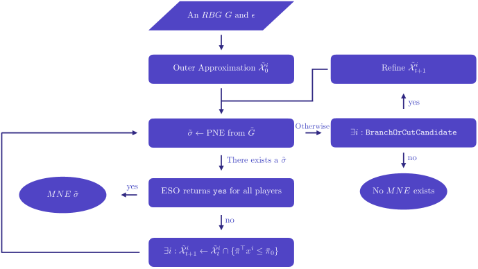
Figure 1: A graphical representation of CnP

4.3.1 Branching may not be enough

The ESO’s cuts of Algorithm 1 are essential for the convergence of CnP. Specifically, a pure branching algorithm (i.e., without cutting) cannot guarantee the separation of an infeasible strategy $\widetilde{\sigma}^{i}$ of $\widetilde{G}$ from $\operatorname{cl}\operatorname{conv}(\mathcal{X}^{i})$. Consider, for instance, the incumbent PNE $\widetilde{\sigma}$ of $\widetilde{G}$ at iteration $t$; the associated strategy $\widetilde{\sigma}^{i}$ of player $i$ may not be an extreme point of $\widetilde{\mathcal{X}}^{i}_{t}$ and, on the contrary, it can be in the interior of $\widetilde{\mathcal{X}}^{i}_{t}$. In this case, the branching operation may not be able to exclude $\widetilde{\sigma}^{i}$ from the refined $\widetilde{\mathcal{X}}^{i}_{t+1}$ (Figure 2). Indeed, finding the correct branching strategy that excludes infeasible strategies may be a hard problem. Consequently, a pure and naive branching-only algorithm might not separate the incumbent PNE of $\widetilde{G}$ from the players’ approximations.

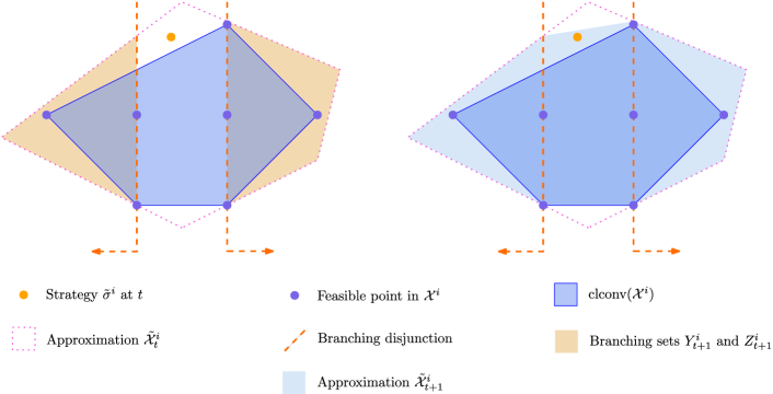
Figure 2: At iteration $t$, branching might not exclude an infeasible PNE from $\widetilde{\mathcal{X}}^{i}_{t+1}$. Given $\widetilde{\sigma}^{i}$ in the interior of $\widetilde{\mathcal{X}}^{i}_{t}$, the branching operation results in a refined $\widetilde{\mathcal{X}}^{i}_{t+1}=\operatorname{cl}\operatorname{conv}(Y^{i}_{t+1}\cup Z^{i}_{t+1})$ that does not exclude $\widetilde{\sigma}^{i}$.

4.3.2 Convergence

We show that CnP terminates in a finite number of iterations with an MNE (or a proof of its non-existence) as long as we can computationally retrieve the description of $\operatorname{cl}\operatorname{conv}(\mathcal{X}^{i})$, for any $i$, in finite time. We formalize this idea in Definition 3.

Definition 3 (Computational Convexifiability).

A set $\mathcal{X}\subseteq\mathbb{R}^{k}$ is computationally convexifiable if either $\mathcal{X}$ is convex or

1. the ESO terminates in a finite number of iterations, and

2. given any initial outer approximation $\widetilde{\mathcal{X}}_{0}\supseteq\mathcal{X}$, we can obtain $\operatorname{cl}\operatorname{conv}(\mathcal{X})$ with a finite sequence of branching steps. In other words, there exists a sequence of approximations $\widetilde{\mathcal{X}}_{0},\widetilde{\mathcal{X}}_{1},\dots,\widetilde{\mathcal{X}}_{T}$ such that $\widetilde{\mathcal{X}}_{t}=\operatorname{cl}\operatorname{conv}\left({Y_{t}}\cup{Z_{t}}\right)$ and ${Y_{t}},\,{Z_{t}}\subseteq\widetilde{\mathcal{X}}_{t-1}$ for any $t>0$, and $\widetilde{\mathcal{X}}_{T}=\operatorname{cl}\operatorname{conv}\left(\mathcal{X}\right)$.

The concept of computational convexifiability formalizes the class of sets for which we can implement an ESO that can compute the sets’ convex hulls; for instance, Examples 2 and 1 deal with computationally-convexifiable sets. If the players’ feasible sets are computationally-convexifiable, we prove, in Theorem 2, that CnP converges; we provide the full proof in the electronic companion.

Theorem 2.

Let $G$ be a polyhedrally-representable SPG. If $\mathcal{X}^{i}$ is computationally convexifiable for each player $i$, then Algorithm 1 terminates in a finite number of steps and 1. if it returns $\widehat{\sigma}=(\widehat{\sigma}^{1},\dots,\widehat{\sigma}^{n})$, then $\widehat{\sigma}$ is an MNE for $G$, and 2. if it returns $\emptyset$, then $G$ has no MNE .

5 The Enhanced Separation Oracle

Let $\mathcal{X}\subseteq\mathbb{R}^{d}$ and $\overline{x}\in\mathbb{R}^{d}$, and assume to have access to an oracle (i.e., a black-box) to optimize a linear function over $\mathcal{X}$ in a computationally-efficient manner. The ESO is an algorithm that, given a point $\overline{x}$, the set $\mathcal{X}$, a numerical tolerance $\epsilon$ and a vector $c\in\mathbb{R}^{d}$:

1. outputs yes and $(V,\alpha)$ if $\overline{x}\in\operatorname{cl}\operatorname{conv}(\mathcal{X})$, with $V\subseteq\mathcal{X}$, and $\alpha\in\mathbb{R}^{|V|}$ being the coefficients of the convex combination of elements in $V$ (i.e., $\overline{x}\in\operatorname{conv}(V)\subseteq\operatorname{cl}\operatorname{conv}(\mathcal{X})$), or

2. outputs no and a tuple $(\overline{\pi},\overline{\pi}_{0})$ so that $\overline{\pi}^{\top}x\leq\overline{\pi}_{0}$ is a cutting plane for $\overline{x}$ and $\operatorname{cl}\operatorname{conv}(\mathcal{X})$, i.e., $\overline{\pi}^{\top}x\leq\overline{\pi}_{0}$ for any $x\in\operatorname{cl}\operatorname{conv}(\mathcal{X})$ and $\overline{\pi}^{\top}\overline{x}>\overline{\pi}_{0}$.

In the above definition, when the ESO outputs no, we separate $\overline{x}$ from $\operatorname{cl}\operatorname{conv}(\mathcal{X})$ via an inequality. Due to Theorem 1, this separation task also has the following game-theoretic interpretation if applied to SPGs; given a set of pure strategies $\mathcal{X}^{i}$ and a point $\widetilde{\sigma}^{i}$, if the ESO returns yes, then $\widetilde{\sigma}^{i}$ is a mixed strategy and $\operatorname{supp}(\widetilde{\sigma}^{i})=V$ with $\alpha$ being the vector of probabilities associated with the strategies in $V$. A theoretical version of this ESO would include polynomially-many runs of the ellipsoid algorithm, which is theoretically viable yet impractical. Therefore, compared to an ellipsoid-based separation oracle [33, 37, 4, 11], we require the numerical tolerance $\epsilon$ and provide a practical implementation. Furthermore, compared to a standard separation oracle, the yes answer from the ESO also describes $\overline{x}$ as a convex combination of points in $\operatorname{cl}\operatorname{conv}(\mathcal{X})$. This last requirement is itself a hard task and, therefore, further motivates the definition of the ESO. Finally, to improve the ESO’s applicability to SPGs, we require the vector $c$ to perform an optimization test that provides a sufficient condition for the ESO to return a no through the idea of value cuts.

5.1 Value Cuts

We start from the concept of equality of payoffs [43, 42], i.e., the concept that, for each player, the payoff of any single pure strategy in the support of an MNE strategy must be equal to the MNE’s payoff. Formally, let $\sigma^{i}$ be a (mixed) best-response for player $i$ given $\sigma^{-i}$. Then, $f^{i}(\sigma^{i};\sigma^{-i})=f^{i}(x^{i};\sigma^{-i})$ for any $x^{i}\in\operatorname{supp}(\sigma^{i})$. We develop an optimization-based test to diagnose the infeasibility of a given strategy in $\widetilde{G}$ with respect to the original SPG $G$. Let $\widetilde{\sigma}=(\widetilde{\sigma}^{1},\dots,\widetilde{\sigma}^{n})$ for $\widetilde{G}$ be the solution to $\widetilde{G}$ at a given CnP iteration. Let $\min_{x^{i}}\{f^{i}(x^{i};\widetilde{\sigma}^{-i}):x^{i}\in\mathcal{X}^{i}\}$ be the best-response problem of $i$ given $\widetilde{\sigma}^{-i}$, and let $\overline{z}^{i}$ be its optimal value. If $\overline{z}^{i}>f^{i}(\widetilde{\sigma}^{i};\widetilde{\sigma}^{-i})$, then $\widetilde{\sigma}^{i}\notin\operatorname{cl}\operatorname{conv}(\mathcal{X}^{i})$, and a valid separating hyperplane for $\operatorname{cl}\operatorname{conv}(\mathcal{X}^{i})$ and $\widetilde{\sigma}^{i}$ is $f^{i}(x^{i};\widetilde{\sigma}^{-i})\geq\overline{z}^{i}$. This follows from the equality of payoffs and that $\overline{z}^{i}$ is the best payoff $i$ can achieve among any pure strategy in $\mathcal{X}^{i}$. We call these separating hyperplanes value cuts. In Proposition 1, we prove such inequalities are valid for the $\operatorname{cl}\operatorname{conv}(\mathcal{X}^{i})$; we provide the proof in the electronic companion.

Proposition 1.

Consider an SPG $G$ and an arbitrary game approximation $\widetilde{G}$ of $G$. Then, for each player $i$ and feasible strategy $\widetilde{\sigma}=(\widetilde{\sigma}^{1},\dots,\widetilde{\sigma}^{n})$ in $\widetilde{G}$, $f^{i}(x^{i};\widetilde{\sigma}^{-i})\geq\inf_{x^{i}}\{f^{i}(x^{i};\widetilde{\sigma}^{-i}):x^{i}\in\mathcal{X}^{i}\}$ is a valid inequality for $\operatorname{cl}\operatorname{conv}(\mathcal{X}^{i})$ if $\inf_{x^{i}}\{f^{i}(x^{i};\widetilde{\sigma}^{-i}):x^{i}\in\mathcal{X}^{i}\}=z^{i}<\infty$. If $z^{i}>f^{i}(\widetilde{\sigma}^{i};\widetilde{\sigma}^{-i})$, we call the inequality a value cut for $\operatorname{cl}\operatorname{conv}(\mathcal{X}^{i})$ and $\widetilde{\sigma}^{i}$.

Finally, because we are outer approximating $\operatorname{cl}\operatorname{conv}(\mathcal{X}^{i})$ for each $i$ and $\widetilde{\sigma}^{i}$ generally comes from the PAG $\widetilde{G}$, it is not possible to have that $z^{i}<f^{i}(\widetilde{\sigma}^{i};\widetilde{\sigma}^{-i})$. In other words, $\widetilde{\sigma}^{i}$ is always a best-response to $\widetilde{\sigma}^{-i}$ in $\widetilde{G}$, yet, it may be infeasible in $G$.

5.2 Implementing the Enhanced Separation Oracle

We provide an implementation of the ESO where we require $\operatorname{cl}\operatorname{conv}(\mathcal{X})$ to be a polyhedron. Our implementation decomposes $\operatorname{cl}\operatorname{conv}(\mathcal{X})$ as a conic combination of its rays $\operatorname{rec}(\operatorname{cl}\operatorname{conv}(\mathcal{X}))$ and convex combination of its extreme points $\operatorname{ext}(\operatorname{cl}\operatorname{conv}(\mathcal{X}))$, i.e., it exploits the so-called $\mathcal{V}$-polyhedral representation of $\mathcal{X}$. The ESO iteratively builds an inner approximation of $\operatorname{cl}\operatorname{conv}(\mathcal{X})$ by keeping track of the rays and vertices. At each ESO’s call, if the input point $\overline{x}$ cannot be expressed by the incumbent inner approximation of $\operatorname{cl}\operatorname{conv}(\mathcal{X})$, the ESO will either improve the inner approximation by including new vertices and rays or output a no. This implementation will also return, in case of a yes, the rays $R$ and the associated conic multipliers $\beta$; in Section 5.3, we will show how to eliminate the conic multipliers and write $\overline{x}$ exclusively as a convex combination of points $\mathcal{X}$.

Data: A point $\overline{x}$, a set $\mathcal{X}$, a tolerance $\epsilon$, a storage of $V,R$, and optionally a vector $c$

Result: Either: (i.) yes and $(V,R,\alpha,\beta)$ if $\overline{x}\in\operatorname{cl}\operatorname{conv}(\mathcal{X})$, or (ii.) no and a separating hyperplane $\overline{\pi}^{\top}x\leq\overline{\pi}_{0}$ for $\operatorname{cl}\operatorname{conv}(\mathcal{X}$) and $\overline{x}$

1 if $c$ was provided  then

2       $\widetilde{x}\leftarrow\arg\min_{x}\{c^{\top}x:x\in\mathcal{X}\}$, with $\overline{z}=c^{\top}\widetilde{x}$

3       if $c^{\top}\overline{x}<\overline{z}$ then  return no and $-c^{\top}x\leq-\overline{z}$

4       if $\|\overline{x}-\widetilde{x}\|<\epsilon$ then  return yes and $(\{\overline{x}\},\emptyset,(1),())$

5      

6 repeat

7       $\mathcal{W}\leftarrow\operatorname{conv}(V)+\operatorname{cone}(R)$. Solve Section 5.2 to determine if $\overline{x}\in\mathcal{W}$ (up to the tolerance $\epsilon$)

8      if $\overline{x}\in\mathcal{W}$  then  return yes and $(V,R,\alpha,\beta)$

9       else

10             $\overline{\pi}^{\top}x\leq\overline{\pi}_{0}$ is a separating hyperplane for $\overline{x}$ and $\mathcal{W}$

11             Let $\mathcal{G}$ be the optimization problem $\max_{x}\{\overline{\pi}^{\top}x:x\in\mathcal{X}\}$

12             if $\mathcal{G}$ is unbounded then  $R\leftarrow R\cup\{r\}$, where $r$ is an extreme ray of $\mathcal{G}$

13             else if $\mathcal{G}$ admits an optimal solution $\nu$ then

14                  

15                  if $\overline{\pi}^{\top}\nu<\overline{\pi}^{\top}\overline{x}$ then  return no and $\overline{\pi}^{\top}x\leq\overline{\pi}^{\top}\nu$

16                   else  $\nu\leftarrow\arg\max_{x}\{\overline{\pi}^{\top}x:x\in\mathcal{X}\}$, and $V\leftarrow V\cup\{\nu\}$

17                  

18            

19      

20

Algorithm 2 Enhanced Separation Oracle

The Algorithm.

Algorithm 2 introduces the implementation of the ESO. This implementation may be warm started with a real-valued vector $c$ to perform the test of Proposition 1; for instance, Algorithm 1 of Algorithm 1 calls the ESO with $c=c^{i}+(C^{i})^{\top}\widetilde{\sigma}^{-i}$, the set $\mathcal{X}^{i}$ of $i$, $\overline{x}=\widetilde{\sigma}^{i}$, and $\epsilon$. As a first step, if $c$ is provided, the algorithm checks if there is any violated value cut by solving the optimization problem $\overline{z}=\min_{x}\{c^{\top}x:x\in\mathcal{X}\}$ of Algorithm 2; specifically, the ESO compares the value of $c^{\top}\overline{x}$ to that of $\overline{z}$. Let $\widetilde{x}$ be the minimizer yielding $\overline{z}$. If 1. $c^{\top}\overline{x}<\overline{z}$(up to the tolerance $\epsilon$), then the ESO returns a value cut (Algorithm 2), or 2. $\|\overline{x}-\widetilde{x}\|<\epsilon$, then the ESO returns yes (Algorithm 2) . Otherwise, let $V$ and $R$ be a set of vertices and rays of $\mathcal{X}$ that the algorithm can store across its iterations. We define $\mathcal{W}$ (Algorithm 2) as the $\mathcal{V}$-polyhedral inner approximation of $\operatorname{cl}\operatorname{conv}(\mathcal{X})$ such that $\mathcal{W}=\operatorname{conv}(V)+\operatorname{cone}(R)$. The central question is then to determine if $\overline{x}\in\mathcal{W}\subseteq\operatorname{cl}\operatorname{conv}(\mathcal{X})$.

The Point-Ray Separator.

To decide if $\overline{x}\in\mathcal{W}$, we formulate a linear program expressing $\overline{x}$ as a convex combination of points in $V$ plus a conic combination of rays in $R$. Let $\alpha$ ($\beta$) be the convex (conic) coefficients for the elements in $V$ ($R$); if $\overline{x}\in\mathcal{W}$, there exists a solution $(\alpha,\beta)$ to

$$\sum_{v\in V}v^{\top}\alpha_{v}+\sum_{r\in R}r^{\top}\beta_{r}=\overline{x},\quad\sum_{v\in|V|}\alpha_{v}=1,\quad\alpha\in\mathbb{R}_{+}^{|V|},\quad\beta\in\mathbb{R}_{+}^{|R|},$$ (4)

where $v$ and $r$ are vertices and rays in $V$, $R$, respectively, and $\alpha_{v}$ and $\beta_{r}$ are their respective convex and conic multipliers. By linear programming duality, 4 has no solution if there exists $(\overline{\pi},\overline{\pi}_{0})$ such that $\overline{\pi}^{\top}\overline{x}-\overline{\pi}_{0}>0$, and

$$\pi v^{\top}-\pi_{0}\leq 0,\quad\pi r^{\top}\leq 0,\quad\forall v\in V,\;\;\forall r\in R.$$ (5)

Practically, we also aim to maximize the violation $\overline{x}^{\top}\pi-\pi_{0}$, and normalize the coefficients $\pi$ so that $||\pi||_{1}=1$. We can equivalently formulate the above requirements as π,π_0, τ_1≥0, τ_2≥0¯x^⊤π-π_0 πv^⊤- π_0≤0  ∀v ∈V,      (α) πr^⊤≤0  ∀r ∈R,      (β) π+τ_1 -τ_2 = 0,    τ_1+τ_2=1 Inspired from Perregaard and Balas [48], Chvátal et al. [11], we define the above program as the Point-Ray Linear Program (PRLP). Each vertex $v\in V$ (resp., ray $r\in R$) requires a constraint as in Section 5.2 (resp., Section 5.2), and the non-negative variables $\tau_{1}$, $\tau_{2}$ represent the $L_{1}$-norm of $\pi$ via Section 5.2. As the program may be unbounded, the normalization constraint Section 5.2 truncates the cone of the PRLP by requiring the $L_{1}$-norm of $\pi$ to be $1$.

Let $\overline{\pi},\overline{\pi}_{0}$ be the optimal values of $\pi,\pi_{0}$. On the one hand, if PRLP admits an optimal solution with an objective of $0$, the oracle returns yes (Algorithm 2) as $\overline{x}\in\mathcal{W}\subseteq\operatorname{cl}\operatorname{conv}(\mathcal{X})$. The convex multipliers $\alpha$ (resp., conic multipliers $\beta$) are the dual values of Section 5.2 (resp., Section 5.2). On the other hand, if $\overline{x}^{\top}\overline{\pi}-\overline{\pi}_{0}>0$ (up to the tolerance $\epsilon$), then $\overline{\pi}^{\top}x\leq\overline{\pi}_{0}$ is a separating hyperplane for $\overline{x}$ and $\mathcal{W}$. To determine if $\overline{\pi}^{\top}x\leq\overline{\pi}_{0}$ is also a separating hyperplane for $\overline{x}$ and $\operatorname{cl}\operatorname{conv}(\mathcal{X})$, the ESO optimizes $\overline{\pi}^{\top}x$ over $\mathcal{X}$ (Algorithm 2). If $\mathcal{G}=\max_{x}\{\overline{\pi}^{\top}x:x\in\mathcal{X}\}$ is unbounded, then its extreme ray $r$ is a new ray for the set $R$. Conversely, if $\mathcal{G}$ admits an optimal solution $\nu$, the latter is a new vertex for the set $V$ (Algorithm 2). Furthermore, if $\overline{\pi}^{\top}\nu<\overline{\pi}^{\top}\overline{x}$, then $\overline{x}$ is infeasible. In practice, this means $\overline{x}$ is separated from $\operatorname{cl}\operatorname{conv}(\mathcal{X})$ by $\overline{\pi}^{\top}x\leq\overline{\pi}^{\top}\nu$, and the ESO returns no. If this is not the case, the ESO identified a new vertex (or ray), and the process restarts from Algorithm 2. We represent Algorithm 2 in Figure 3.

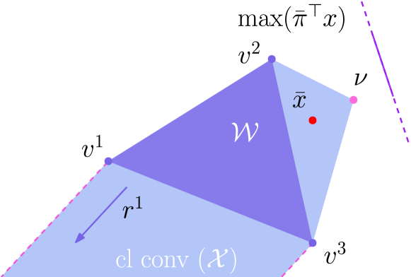
(a) $\nu\notin\mathcal{W}$. Optimizing $\overline{\pi}^{\top}x$ over $\mathcal{X}$ yields $\nu$. In the next iteration, the ESO will returns yes, as $\overline{\pi}^{\top}\nu>\overline{\pi}^{\top}\overline{x}$.

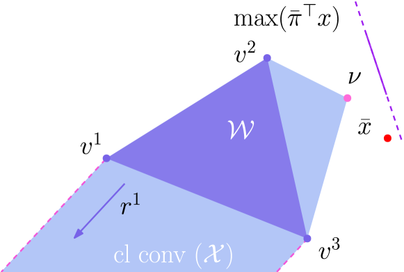
(b) $\nu\notin\mathcal{W}$. Optimizing $\overline{\pi}^{\top}x$ over $\mathcal{X}$ yields $\nu$. In the next iteration, the ESO will return no and $\overline{\pi}^{\top}\nu<\overline{\pi}^{\top}\overline{x}$.

Figure 3: A 2-dimensional example of Algorithm 2 separating $\overline{x}$ from $\operatorname{cl}\operatorname{conv}(\mathcal{X})$. Here, $\mathcal{X}=\{\operatorname{conv}(\{v^{2},\nu\})\}\bigcup\{\operatorname{conv}(\{v^{1},v^{3}\})+\operatorname{cone}(\{r^{1}\})\}$. The set $\operatorname{cl}\operatorname{conv}(\mathcal{X})$ is the light-blue region, whereas its inner approximation $\mathcal{W}=\operatorname{conv}(\{v^{1},v^{2},v^{3}\})$ is in purple.

Practical Considerations.

First, similarly to Perregaard and Balas [48], we can modify Algorithm 2 of Algorithm 2 to retrieve multiple vertices and rays violating $\overline{\pi}^{\top}x\leq\overline{\pi}_{0}$, and subsequently add them in Algorithm 2 and Algorithm 2. In this way, the inner approximation $\mathcal{W}$ tends to build faster without significantly impacting the computational overhead. Second, the normalizations of the PRLP in Section 5.2 are practically pivotal as they affect the algorithm’s overall stability (and convergence) through the generated cutting planes. Because normalizations tend to affect the generators’ performance significantly (see, e.g., Dey et al. [21], Fischetti et al. [30], Bixby [3], Perregaard and Balas [48]), we normalize Section 5.2 with Section 5.2. Finally, in Theorem 3, we show that our implementation of the ESO terminates in a finite number of steps; we defer the proof to the electronic companion.

Theorem 3.

The ESO terminates in a finite number of steps if $\operatorname{cl}\operatorname{conv}(\mathcal{X})$ is a polyhedron.

5.3 Eliminating the Conic Coefficients

In Theorem 1, we interpret any convex combination of strategies in $\mathcal{X}^{i}$ in a game-theoretic fashion, i.e., as a mixed strategy for player $i$, where each element in the convex combination is a pure strategy whose probability of being played is given by the associated convex combination’s coefficient. However, Algorithm 2 returns, whenever the answer is yes, a proof of inclusion $(V,R,\alpha,\beta)$ that also includes a conic combination of the extreme rays in $R$. As the game-theoretic interpretability of the solution given by CnP is fundamental, especially when players solve unbounded problems, we provide a simple algorithm to repair a proof of inclusion $(V,R,\alpha,\beta)$ to a proof of inclusion $(V,\alpha)$ that does not include any conic combination. We illustrate its intuition in Figure 4.

Example 5 (Conic Combinations).

Consider the example in Figure 4, and assume that Algorithm 2 returns yes, and a proof of inclusion $(V,R,\alpha,\beta)$. Let $V$ be $\{v^{1},v^{2}\}$, $R$ be $\{r^{1}\}$, and $\mathcal{W}$ be $\operatorname{conv}(V)+\operatorname{cone}(R)$. Let $\mathcal{X}$ be made by the points $\{v^{1},v^{2},v^{3}\}$ and the sequence of points $v^{3,1},v^{3,2},\dots$ along $r^{1}$. Although the proof of inclusion of $\overline{x}$ employs the ray $r^{1}$, we can equivalently express $\overline{x}$ as a convex combination of $v^{1}$, $v^{2}$ and $v^{3,1}$ without resorting to $r^{1}$.

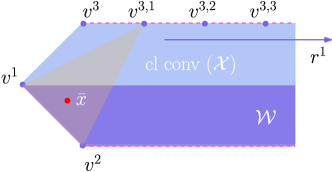
Figure 4: Rewriting $\overline{x}$ as a convex combination of $v^{1}$, $v^{2}$ and $v^{3,2}$ (orange area).

A Repair Algorithm.

If CnP terminates with an MNE that includes rays, Algorithm 3 provides the repairing routine that eliminates the rays from the proof of inclusion of each player $i$. Algorithm 3 requires the point $\overline{x}\in\operatorname{cl}\operatorname{conv}(\mathcal{X})$, the set $\mathcal{X}$, a numerical tolerance $\epsilon$, an arbitrarily-large constant $B\in\mathbb{R}$ and the proof of inclusion $(V,R,\alpha,\beta)$ from the ESO of Algorithm 2. Algorithm 3 iteratively attempts to express $\overline{x}$ as a convex combination of points in $V$ by augmenting $V$ with some points (not necessarily extreme points) of $\mathcal{X}$. Initialize $\widetilde{V}$ as $V$. At each iteration, the algorithm augments $\widetilde{V}$ with the optimal solutions of $\max_{x}\{r^{\top}x:x\in\mathcal{X},r^{\top}x\leq B\}$ for any $r\in R$ (Algorithm 3). If $\overline{x}\in\widetilde{V}$ due to the PRLP of Algorithm 3, then the algorithm returns $(\widetilde{V},\widetilde{\alpha})$, where $\widetilde{\alpha}$ are the dual variables of the PRLP. Otherwise, the algorithm increments $B$ and keeps iterating. We remark that Algorithm 3 terminates in a finite number of iterations, as $x\in\operatorname{cl}\operatorname{conv}(\mathcal{X})$, and there exists a $B^{\prime}$ such that $r^{\top}x\leq B^{\prime}$ for any $r\in R$ and $x\in\mathcal{X}$.

Data: A point $\overline{x}$, $\mathcal{X}$, a tolerance $\epsilon$, a large $B\in\mathbb{R}$, and $(V,R,\alpha,\beta)$ from Algorithm 2

Result: A proof of inclusion $(V,\alpha)$

1 repeat

2       $\widetilde{V}\leftarrow V$

3       for $r\in R$ do  $\nu\leftarrow\arg\max_{x}\{r^{\top}x:x\in\mathcal{X},r^{\top}x\leq B\}$, and $\widetilde{V}\leftarrow\widetilde{V}\cup\{\nu\}$

4       Solve the PRLP Section 5.2 to determine if $\overline{x}\in\operatorname{conv}(\widetilde{V})$ (up to the tolerance $\epsilon$)

5       if $\overline{x}\in\operatorname{conv}(\widetilde{V})$ then  return yes and $(\widetilde{V},\widetilde{\alpha})$ else increase $B$

6      

7

Algorithm 3 Repairing Algorithm

6 Applications

In this section, we evaluate CnP on two challenging nonconvex games, demonstrate the algorithm’s effectiveness and establish a solid computational benchmark against the literature. We consider IPGs and NASPs, i.e., two classes of games among players solving integer and bilevel problems. In both cases, determining the existence of an equilibrium is generally $\Sigma^{p}_{2}$-hard; therefore, we expect the computation of an equilibrium, or the determination of its non-existence, to be challenging. We compare CnP against the most advanced problem-specific algorithms and empirically demonstrate that our algorithm is scalable and efficient and can also exploit problem-specific structures.

Reciprocally-bilinear Games.

In our tests, we focus on Reciprocally-Bilinear Games (RBGs), a subclass of SPG where each player’s payoff function is linear in its variables.

Definition 4 (Reciprocally-Bilinear Game).

An RBG is an SPG where each player $i$’s payoff function is reciprocally-bilinear, i.e., $f^{i}(x^{i};x^{-i}):=(c^{i})^{\top}x^{i}+(x^{-i})^{\top}C^{i}x^{i}$ and $C^{i}$ is a real-valued matrix.

Compared to SPG, determining if a PAG $\widetilde{G}$ admits an MNE in a RBG is equivalent to solving an Linear Complementarity Problem (LCP), as opposed to an NCP. Although there are specialized LCP solvers (e.g., PATH from Dirkse and Ferris [22], Ferris and Munson [29]), there are also well-known MIP reformulations [38]. Despite a MIP reformulation does not exploit the underlying complementarity structure, MIP solvers can optimize several computationally-tractable functions over the set of the LCP’s solutions and, therefore, select an MNE in the PAG $\widetilde{G}$ that maximizes a given objective function. In this sense, CnP supports heuristic equilibria selection and enables the user to select the preferred balance between equilibrium quality (i.e., given a function that measures its quality) with the time required for its computation. In our tests, we employ Gurobi 9.2 as MIP solver and PATH as an LCP solver. We report all the time-related results as shifted geometric means with a shift of $10$ seconds.

6.1 Integer Programming Games

We consider a class of IPGs where each player $i$ solves the parametrized integer program

$$\max_{x^{i}}\big{\{}(c^{i})^{\top}x^{i}+(x^{-i})^{\top}C^{i}x^{i}\quad\text{subject to}\quad A^{i}x^{i}\leq b^{i},\quad x^{i}\geq 0,\quad x^{i}_{j}\in\mathbb{Z}\quad\forall j\in\mathcal{I}^{i}\big{\}}.$$ (6)

The matrix $A^{i}$ and the vector $b^{i}$ have rational entries for any $i$, and $\mathcal{I}^{i}$ contains the indexes of the integer-constrained variables. Reciprocally-bilinear IPGs have applications in several domains, e.g., revenue management, healthcare, cybersecurity, and sustainability [17, 25, 5], and can also represent any 2-player normal-form game; we refer to Carvalho et al. [10] for a tutorial.

Customizing CnP.

We tailor Algorithm 1 as follows:

1. The set $\operatorname{cl}\operatorname{conv}(\mathcal{X}^{i})$ is the so-called perfect formulation of $\mathcal{X}^{i}$ [13], and any family of valid inequalities for an integer program is also valid for each player $i$’s $\operatorname{cl}\operatorname{conv}(\mathcal{X}^{i})$. In our tests, we customize CnP by employing some families of MIP cutting planes. Specifically, we use Gomory Mixed-Integer (GMIs), Mixed-Integer Rounding (MIRs), and Knapsack Cover (KPs) inequalities through the software CoinOR Cgl [12]. We refer the reader to [14] for a description of these inequalities. Finally, at iteration $t=0$ of CnP, we let each $\widetilde{\mathcal{X}}^{i}_{0}$ be the associated linear relaxation.

2. If the ESO in Algorithm 1 returns no at iteration $t$, we add an additional valid inequalities to refine $\widetilde{\mathcal{X}}^{i}_{t+1}$. Furthermore, whenever the value cuts do not exhibit a well-behaved numerical behavior (e.g., fractional coefficients with several decimal digits), we attempt to replace them with a valid inequality from (i.).

6.1.1 Computational Tests

Instances and Parameters.

We compare CnP with the SGM algorithm of Carvalho et al. [8], the most efficient algorithm to compute an MNE in IPG with mixed-integer variables. We employ the popular instances of the knapsack game, where each player $i$ solves a knapsack problem with $m$ items; namely, each player $i$ has a set of strategies $\mathcal{X}^{i}=\big{\{}w^{i}x^{i}\leq\overline{w}^{i},\;\;x^{i}\in\{0,1\}^{m}\big{\}}$. The parameters $c^{i}\in\mathbb{Z}^{m}$ and $w^{i}\in\mathbb{Z}^{m}_{+}$ are integer vectors representing the profits and weights of player $i$, respectively; The parameter $\overline{w}^{i}$ is the knapsack capacity, whereas $C^{i}\in\mathbb{Z}^{m\times(n-1)m}$ is a diagonal matrix. The elements on the diagonal are the so-called interaction coefficients associated with each of the $(n-1)$ other players in the game and their $m$ decision items (in the lexicographic order given by each player’s index). Thus, players interact only when selecting corresponding items, i.e., $x^{i}_{j}$ and $x^{o}_{j}$ for $i,o\in\{1,\dots,n\}$. We remark that the entries of $C^{i}$ are integer-valued but not necessarily positive, i.e., the interaction for a given item can be positive or negative, and $C^{i}$ are different among players.

Because, in any PAG, players optimize convex functions over convex and compact feasible regions, any PAG admits a PNE and CnP purely acts as a cutting plane algorithm. We solve the LCPs in 3 with either: 1. PATH, thus computing a feasible MNE for each PAG, or 2. Gurobi, by optimizing the quadratic social welfare function $SW(\sigma)=\sum_{i=1}^{n}f^{i}(\sigma^{i};\sigma^{-i})$, i.e., the sum of the players’ payoffs. When optimizing the social welfare, we aim to find equilibria exhibiting desirable properties from the perspective of a regulator, i.e., we aim to heuristically select the equilibria that favor the players and a hypothetical third-party regulator the most. Finally, we set $\epsilon=3\times 10^{-5}$, a time limit of $300$ seconds, and we employ the $70$ instances from Carvalho et al. [8], where $n\in\{2,3\}$ and $10\leq m\leq 100$.

Results.

Table 1 provides an aggregate overview of the results by categorizing the instances in two sets: the small instances (i.e., $mn\leq 80$) in rows $2-8$, and the large ones (i.e., $mn>80$) in rows $9-15$. The first column reports the algorithm, where, for CnP, we specify whether we use Gurobi or PATH (resp., CnP-Gurobi and CnP-PATH). Column O is the objective type, either F for feasibility or Q when CnP optimizes $SW$ while solving each PAG. Column C reports the aggressiveness of the additional MIP inequalities generated. Specifically C can be: 1. $-1$if CnP do not use MIP cuts, or 2. $0$if it adds MIP cuts to replace numerically-unstable value cuts, or 3. $1$if it concurrently adds MIP cuts on top of numerically-stable value cuts. The columns Time and #TL report the time in seconds and the number of time limit hits, respectively. Column MinMax reports the absolute difference (in seconds) between the maximum and the minimum computing time. Column SW% reports the average social welfare improvement compared to the MNE computed by SGM. Finally, in the remaining columns, we report the average number of iterations (#It), cuts added (Cuts), and MIP cuts (MIPCuts). We remark that Cuts includes any cut from the ESO (including value cuts) and the MIP cuts.

Discussion.

CnP always computes equilibria with remarkably modest computing times. Furthermore, CnP improves the average social welfare compared to SGM; this is mainly due to the algorithm’s approximation structure: whereas SGM approximates the player’s strategy sets from the inside, CnP outer approximates them and thus has a larger search space. The social welfare improves when CnP leverages a MIP solver, with the average welfare values almost doubling. However, this improvement tends to increase the computing times as MIP solvers cannot exploit the structure of 3. When CnP uses PATH, there are dramatic computing time improvements over the whole set of instances. Furthermore, the more MIP cuts, the fewer iterations are required to converge to an MNE. When combining CnP with MIP cuts, we generally observe a reduction in the computing time and a lower MinMax value. Finally, we remark that despite our instances being as large as the ones considered in Dragotto and Scatamacchia [23], Carvalho et al. [8], Crönert and Minner [17], CnP exhibits limited computing times.

Algorithm	O	C	Time (s)	MinMax	#TL	SW%	#It	Cuts	MIPCuts
SGM			0.73	21.43	0	0.0%	8.43	-	-
CnP-MIP	Q	-1	6.58	287.52	0	13.5%	7.80	9.57	0.00
CnP-MIP	Q	0	6.13	287.01	0	12.9%	5.73	6.47	2.30
CnP-MIP	Q	1	6.31	287.52	0	13.3%	3.50	9.60	7.47
CnP-PATH	F	-1	0.36	10.54	0	1.8%	7.60	10.2	0.00
CnP-PATH	F	0	0.05	0.19	0	2.9%	5.27	5.90	2.07
CnP-PATH	F	1	0.04	0.19	0	4.9%	3.23	8.87	7.10
SGM			20.86	300.00	6	0.0%	18.58	-	-
CnP-MIP	Q	-1	61.08	294.50	0	22.5%	13.70	17.00	0.00
CnP-MIP	Q	0	57.85	299.45	1	19.6%	11.62	12.62	3.45
CnP-MIP	Q	1	68.20	299.04	0	22.3%	9.48	16.80	10.32
CnP-PATH	F	-1	6.68	80.89	0	15.7%	13.55	16.35	0.00
CnP-PATH	F	0	4.48	74.37	0	15.7%	9.62	10.25	2.42
CnP-PATH	F	1	4.32	75.88	0	15.9%	8.22	14.35	8.43

Table 1: IPGs results on the knapsack game. Extended results are available in the electronic companion.

6.2 Nash Games Among Stackelberg Players

NASPs [9] are SPGs where each player $i$ solves a bilevel problem, i.e., a multi-level optimization problem. This family of games is instrumental in energy and pricing, as it represents complex systems of hierarchical interaction and combines simultaneous and sequential interactions. In a NASP, each player $i$ solves

$$\min_{x^{i}}\quad x^{i}(c^{i})^{\top}x^{i}+\sum_{o=1,o\neq i}^{n}(x^{o})^{\top}Q^{i}_{o}x^{i}$$ (7a)

subject to $$A^{i}x^{i}\leq b^{i},\quad x^{i}\geq 0,\quad\;x^{i}=(w^{i},\widehat{y}^{i}),\quad\widehat{y}^{i}\in\text{SOL}(w^{i}),$$ (7b)

where $x^{i}$ is partitioned into the leader’s variables $w^{i}$, and the followers’ variables $y^{i}$. For each player $i$, there are $u_{i}$ followers controlling the variables $y^{i,j}$ with $j=1,\dots,u_{i}$ and solving a convex quadratic optimization problem in $y^{i,j}$ parametrized in $w^{i}$. The set $\text{SOL}(w^{i})$ in 7b represents the solutions $y^{i}=(y^{i,1},\dots,y^{i,u_{i}})$ to the $i$-th player lower-level simultaneous game. Therefore, the feasible set $\mathcal{X}^{i}$ for each player is given by a set of linear constraints 7b plus the optimality of the followers’ game 7b. The feasible region $\mathcal{X}^{i}$ of each player is a finite union of polyhedra [9], and thus NASPs are polyhedrally-representable RBGs. Indeed, we can express $\mathcal{X}^{i}$ as

$$\mathcal{X}^{i}=\underbrace{\{A^{i}x^{i}\leq b^{i},z^{i}=M^{i}x^{i}+q^{i},x^{i}\geq 0,z^{i}\geq 0\}}_{\mathcal{X}^{i}_{0}}\bigcap_{j\in\mathcal{C}^{i}}(\{z^{i}_{j}=0\}\cup\{x^{i}_{j}=0\}),$$ (8)

where $\mathcal{C}^{i}$ is a set of indexes for the complementarity equations that equivalently express $\text{SOL}(w^{i})$. For any player $i$, we refer to $\mathcal{X}^{i}_{0}$ in 8 as its polyhedral relaxation. In other words, $\mathcal{X}^{i}_{0}$ is the polyhedron containing the leader constraints, the definitions for $z^{i}$, and the non-negativity constraints. Because $\operatorname{cl}\operatorname{conv}(\mathcal{X}^{i})$ may be unbounded, an MNE in NASPs might not exist.

Customizing CnP.

We express each player’s program by reformulating $\mathcal{X}^{i}$ as in 8. In CnP, the initial relaxation of Algorithm 1 is the polyhedral relaxation $\widetilde{\mathcal{X}}^{i}_{0}$ for each player $i$, i.e., the feasible region where we omit all the complementarity constraints. As the description of 8 only needs a finite number of complementarity conditions in $\mathcal{C}^{i}$, the branching step account for finding the disjunction associated with the complementarity condition $z^{i}_{j}=0$ or $x^{i}_{j}=0$. Let $J^{i}_{t}$ be the set of disjunctions added at iteration $t$ of the algorithm. Then, Algorithm 1 will include in $\widetilde{\mathcal{X}}^{i}_{t+1}$ at least one complementarity $j$ for some player $i$ so that $j\in\mathcal{C}^{i}\backslash J^{i}_{t}$. This boils down to the computation of $\widetilde{\mathcal{X}}^{i}_{t+1}$ as the union of a two-sided disjunction $\{\widetilde{\mathcal{X}}^{i}_{t}\cap x^{i}_{j^{i}}\leq 0\}$ and $\{\widetilde{\mathcal{X}}^{i}_{t}\cap z^{i}_{j^{i}}\leq 0\}$, where $x^{i}_{j^{i}}$,$z^{i}_{j^{i}}$ are the terms involved in the $j$-th complementarity of $i$. If, at some iteration $t$, $J^{i}_{t}=\mathcal{C}^{i}$ for any $i$, then $\operatorname{cl}\operatorname{conv}(\mathcal{X}^{i})=\widetilde{\mathcal{X}}^{i}_{t}$ and the algorithm terminates. Furthermore, we develop two custom branching rules for NASPs. Assume a PAG admits an MNE $\widetilde{\sigma}$ at iteration $t-1$ and needs to determine the best branching candidate in $\mathcal{C}^{i}\backslash J^{i}_{t}$ at iteration $t$; we propose two branching rules:

1. Hybrid branching. For any candidate set $\mathcal{C}^{i}\backslash J^{i}_{t}$, we would like to select the candidate $j$ that minimizes the distance between $\widetilde{\sigma}^{i}$ and the set $\widetilde{\mathcal{X}}^{i}_{t+1}$ that includes the $j$-th complementarity. Therefore, we select $j$ by solving $\min_{\lambda^{i}}\{(\lambda^{i})^{2}:\widetilde{\sigma}^{i}\in\operatorname{cl}\operatorname{conv}(\{\widetilde{\mathcal{X}}^{i}_{t}\cap x^{i}_{j^{i}}\leq 0\}\cup\{\widetilde{\mathcal{X}}^{i}_{t}\cap z^{i}_{j^{i}}\leq 0\})\}$, where $\lambda$ is the vector of violations associated with each constraint in $\widetilde{\mathcal{X}}^{i}_{t}$ plus the disjunctions on the $j$-th complementarity candidate.

2. Deviation branching. We solve the best-response problem of $i$ given $\widetilde{\sigma}^{-i}$, and compute an optimal solution $\widetilde{x}^{i}$. Then, we select the first (given an arbitrary order) candidate $j$ that encodes the polyhedron containing $\widetilde{x}^{i}$.

6.2.1 Computational Tests

Instance and Parameters.

We set $\epsilon=10^{-5}$, and consider a time limit of $300$ seconds. We employ the $50$ instances InstanceSet B from Carvalho et al. [9], where each instance has $7$ players with up to $3$ followers each, and compare against the problem-specific (sequential) inner approximation algorithm (Inn-S) from Carvalho et al. [9]. We also introduce $50$ harder instances H7 with $7$ players with $7$ followers each. Large NASPs instances, such as the H7 set, are generally numerically badly scaled and thus helpful to perform stress tests on the numerical stability of algorithms.

Results and Discussion.

We report the aggregated results in Table 2. The first column reports the type of algorithm: the baseline (Inn-S) or CnP with either the hybrid (HB) or deviation (DB) branching. Furthermore, we test Inn-S-1 and Inn-S-3, two configurations of the inner approximation algorithm (we refer to the original paper for a detailed description). The second columns report the instance set (Inst), i.e., either B or H7. The three subsequent pairs of columns report the average computing time (Time) and the number of instances (#) for which the algorithm either: 1. found an MNE (EQ), or 2. proved that no MNE exists (NO_EQ), or 3. terminated with either an MNE or a proof of its non-existence without exhibiting numerical issues (ALL) . The last two columns report the number of numerical issues (#NI) and time limit hits (#TL) each algorithm encountered. The baseline Inn-S-1 systematically fails on the set H7 due to the size of the descriptions of $\operatorname{cl}\operatorname{conv}(\mathcal{X}^{i})$. Indeed, Inn exhibits significant numerical issues in the set H7, even though the former is a problem-specific algorithm. On the contrary, CnP performs consistently and is especially effective in the hard set H7. The running times of both algorithms are comparable in the smaller instance set B, and CnP is competitive with Inn while not being a problem-specific algorithm.

Table 2: NASPs results.

Algo	Inst	Time (s)	#	Time (s)	#	Time (s)	#N	#NI	#TL
		EQ		NO_EQ		ALL
Inn-S-1	B	6.22	49	69.76	1	6.56	50	0	0
Inn-S-3	B	4.94	49	23.96	1	5.12	50	0	0
CnP-HB	B	7.47	46	29.37	1	7.71	47	3	0
CnP-DB	B	9.45	46	11.81	1	9.50	47	3	0
Inn-S-1	H7	-	0	-	0	300.00	46	4	46
Inn-S-3	H7	-	0	-	0	-	0	50	0
CnP-HB	H7	53.79	41	-	0	73.45	50	0	9
CnP-DB	H7	52.58	35	-	0	88.92	50	0	15

7 Concluding Remarks

In this work, we presented CnP, an efficient algorithm for computing Nash equilibria in SPGs, a large class of non-cooperative games where players solve nonconvex optimization problems. We showed that nonconvex SPGs admit equivalent convex formulations where the players’ feasible sets are the closure of the convex hulls of their original nonconvex feasible regions. Starting from this result, we designed CnP, a cutting-plane algorithm to compute exact MNEs in SPGs or certify their non-existence. We defined the concept of game approximation and employed it through CnP by building an increasingly accurate sequence of convex approximations converging to an equilibrium or a certificate of its non-existence. Our algorithm is exact, problem-agnostic, and exhibits solid computational performance. Although CnP is a general-purpose algorithm, we also demonstrated how to tailor it to exploit the structure of specific classes of games.

Given the generality of our algorithm, we prudently believe improvement opportunities lie ahead. We hope our contribution can inspire future methodological development in equilibria computation in nonconvex games. Among those, we foresee an extension of our methodology beyond the assumption of polyhedral representability. Finally, as Nash equilibria play a pivotal role in designing and regulating economic markets, we hope our algorithm will enable economists and optimizers to design complex markets stemming from sophisticated economic models.

Electronic Companion

8 Proof of Theorem 2.

Proof of Theorem 2..

Finite Termination. We show that CnP terminates in a finite number of iterations. The calls to solve the NCP in Algorithm 1, and to the ESO in Algorithm 1 terminate in a finite number of steps because we assume the players’ feasible sets are computationally-convexifiable. The only loop that could potentially not terminate is the repeat starting in Algorithm 1.

First, we restrict to the case where the set $\mathcal{X}^{i}$ is bounded or finite for any player $i$. Any PAG $\widetilde{G}$ will necessarily admit a PNE if the approximations $\widetilde{\mathcal{X}}^{i}_{t}$ are also bounded; therefore, the algorithm will never trigger Algorithm 1. Thus, Algorithm 1 is the only step refining the sets $\widetilde{\mathcal{X}}^{i}_{t}$ for some player $i$. As $\mathcal{X}^{i}$ is computationally-convexifiable for every player $i$, the ESO can, in a finite number of steps, refine the approximations $\widetilde{\mathcal{X}}^{i}_{t}$ to $\operatorname{cl}\operatorname{conv}(\mathcal{X}^{i})$. As a consequence, the algorithm converges (in the worst case) to $\overline{G}$ (i.e., the exact convex approximation), and the correctness of the resulting MNE follows from Theorem 1.

Second, if $\mathcal{X}^{i}$ is unbounded for some player $i$, then a PNE for a given PAG $\widetilde{G}$ may not exist, and the algorithm may enter Algorithm 1. However, because $\mathcal{X}^{i}$ is computationally-convexifiable for every player $i$, the branching step and the ESO can refine, in a finite number of steps, the approximations $\widetilde{\mathcal{X}}^{i}_{t}$ to $\operatorname{cl}\operatorname{conv}(\mathcal{X}^{i})$. Therefore, even in the unbounded case, the algorithm correctly returns an MNE, similarly to the bounded case.

Proof of statements (i) and (ii). We show that $\widehat{\sigma}$ is an MNE for $G$. If the algorithm returns $\widehat{\sigma}$, there exists an approximate game $\widetilde{G}$ in Algorithm 1 with a PNE $\widetilde{\sigma}=\widehat{\sigma}$. Let the iteration associated with $\widetilde{G}$ having a PNE $\widehat{\sigma}$ be denoted with $t=\theta$, and, for each player $i$, let $\widetilde{\mathcal{X}}^{i}_{\theta}$ be the associated feasible region $i$. Then, for any player $i$ and $\overline{\sigma}^{i}\in\widetilde{\mathcal{X}}^{i}_{\theta}$, it follows that $f^{i}(\widehat{\sigma}^{i};\widehat{\sigma}^{-i})\leq f^{i}(\overline{\sigma}^{i};\widehat{\sigma}^{-i})$, i.e., no player $i$ has the incentive to deviate from $\widehat{\sigma}^{i}$ to any other strategy $\overline{\sigma}^{i}\in\widetilde{\mathcal{X}}^{i}_{\theta}$ in $\widetilde{G}$. Because $\operatorname{cl}\operatorname{conv}(\mathcal{X}^{i})\subseteq\widetilde{\mathcal{X}}^{i}_{\theta}$ for any $i$, then the previous inequality holds for any $\overline{\sigma}^{i}\in\operatorname{cl}\operatorname{conv}(\mathcal{X}^{i})$. Moreover, by construction, $\widehat{\sigma}^{i}\in\operatorname{cl}\operatorname{conv}(\mathcal{X}^{i})$; otherwise, the ESO would have returned no for player $i$. ∎

9 Proof of Theorem 3.

Proof of Theorem 3..

The ESO inner approximates the polyhedron $\operatorname{cl}\operatorname{conv}(\mathcal{X})$ with its $\mathcal{V}$-representation, which is made of finitely many extreme rays and vertices. Hence, we have to prove that the ESO will never find, at any step, a vertex $\nu$ (ray $r$) in Algorithm 2 (Algorithm 2) so that $\nu$ is already in $V$ ($r$ is already in $R$). This implies that the repeat loop in Algorithm 2 terminates.

The inequality in Algorithm 2 is valid for $\mathcal{W}$ if and only if $\overline{\pi}^{\top}v\leq\overline{\pi}_{0}$ for any $v\in V$, and $\overline{\pi}^{\top}r\leq 0$ for any $r\in R$ as of Section 5.2 and Section 5.2. Also, because the latter inequality is a separating hyperplane between $\mathcal{W}$ and $\overline{x}$, then $\overline{\pi}^{\top}\overline{x}>\overline{\pi}_{0}$; however, it may not necessarily be a valid inequality for any element in $\operatorname{ext}(\operatorname{cl}\operatorname{conv}(\mathcal{X}))$ and $\operatorname{rec}(\operatorname{cl}\operatorname{conv}(\mathcal{X}))$. Therefore, we must consider the optimization problem $\mathcal{G}$ in Algorithm 2. On the one hand, if $\mathcal{G}$ is bounded, let $\nu$ be its optimal solution. Then, either 1. $\overline{\pi}^{\top}\nu<\overline{\pi}^{\top}\overline{x}$, with $\overline{\pi}^{\top}x\leq\overline{\pi}^{\top}\nu$ being a separating hyperplane between $\operatorname{cl}\operatorname{conv}(\mathcal{X})$ and $\overline{x}$, and the algorithm terminates and returns no, or 2. $\overline{\pi}^{\top}\nu\geq\overline{\pi}^{\top}\overline{x}$, $\nu$ is necessarily a vertex of $\operatorname{ext}(\operatorname{cl}\operatorname{conv}(\mathcal{X}))\backslash V$ violating $\overline{\pi}^{\top}x\leq\overline{\pi}_{0}$, and the algorithm updates $V\leftarrow V\cup\{\nu\}$ . On the other hand, if $\mathcal{G}$ is unbounded, then there exists an extreme ray $r$ so that $\overline{\pi}^{\top}r>0$. Then, $r$ is necessarily in $\operatorname{rec}(\operatorname{cl}\operatorname{conv}(\mathcal{X}))\backslash R$, $\overline{\pi}^{\top}r>\overline{\pi}_{0}$, and the algorithm updates $R\leftarrow R\cup\{r\}$ and returns to Algorithm 2. As there are finitely many extreme rays and vertices, the algorithm will then terminate. ∎

10 Proof of Proposition 1

Proof of Proposition 1..

If the infimum is attained at a finite value $z^{i}$, this implies that player $i$ cannot achieve a payoff strictly less than $z^{i}$ given the other players’ strategies $\widetilde{\sigma}^{-i}$; in other words, $z^{i}$ is the payoff associated with the best response of $i$ to $\widetilde{\sigma}^{-i}$. Consider the problem

$$\inf_{x^{i}}\{f^{i}(x^{i};\widetilde{\sigma}^{-i}):x^{i}\in\operatorname{cl}\operatorname{conv}(\mathcal{X}^{i})\}.$$ (9)

The above problem attains a finite infimum because $z^{i}$ is finite. Let $\overline{v}^{i}$ be an optimal solution, i.e., a best response, and $\overline{z}^{i}$ be the finite optimal value of 9, respectively. We claim that $z^{i}=\overline{z}^{i}$ for any $\overline{v}^{i}\in\operatorname{cl}\operatorname{conv}(\mathcal{X}^{i})$ that solves 9. On the one hand, assume that $\overline{z}^{i}<z^{i}$. Note that $\overline{v}^{i}\in\operatorname{cl}\operatorname{conv}(\mathcal{X}^{i})$ is a convex combination of points in $\mathcal{X}^{i}$, and $f^{i}(x^{i};\widetilde{\sigma}^{-i})$ is linear in $x^{i}$. Then, any point $\widehat{v}^{i}$ involved in the convex combination resulting in $\overline{v}^{i}$ belongs to $\mathcal{X}^{i}$; this also imply that $z^{i}$ is not the optimal value of $\inf_{x^{i}}\{f^{i}(x^{i};\widetilde{\sigma}^{-i}):x^{i}\in\mathcal{X}^{i}\}$, resulting in a contradiction. On the other hand, assume that $\overline{z}^{i}>z^{i}$. Because the solutions to $\inf_{x^{i}}\{f^{i}(x^{i};\widetilde{\sigma}^{-i}):x^{i}\in\mathcal{X}^{i}\}$ are also feasible for 9, $\overline{v}^{i}$ cannot be a minimizer of 9. ∎

11 IPGs Results

Tables 3 and 4 presents the full computational results for our experiments. The column names are analogous to those of Table 1, with the addition of a few columns. Specifically, we report the value of the social welfare in SW and the average numbers of: 1. cuts from the ESO excluding value cuts (ESOCuts), 2. value cuts from the ESO (VCuts). Finally, in the time column, we report in parenthesis the time the algorithm spent to compute the first MNE; this is relevant when CnP optimizes the social welfare function via a MIP solver.

Table 3: IPGs complete results, first set.

Algorithm	O	C	Time (s)	#TL	SW	#It	Cuts	ESOCuts	VCuts	MIPCuts
n=3 m=10
SGM	-	-	2.11	0	632.99	10.00	-	-	-	-
CnP-MIP	Q	-1	0.47 (0.23)	0	812.48	4.50	5.0	2.0	3.0	0.0
CnP-MIP	Q	0	0.31 (0.14)	0	812.98	4.60	4.8	2.0	1.1	1.7
CnP-MIP	Q	1	0.20 (0.08)	0	820.71	2.60	7.2	0.5	1.1	5.6
CnP-PATH	F	-1	0.02	0	706.66	5.00	5.9	2.0	3.9	0.0
CnP-PATH	F	0	0.02	0	718.13	4.50	4.9	2.0	1.5	1.4
CnP-PATH	F	1	0.03	0	742.87	2.00	5.4	0.3	0.7	4.4
n=2 m=20
SGM	-	-	0.01	0	658.31	5.40	-	-	-	-
CnP-MIP	Q	-1	0.96 (0.25)	0	684.19	6.40	6.3	4.4	1.9	0.0
CnP-MIP	Q	0	0.93 (0.29)	0	683.91	6.10	5.9	3.0	1.2	1.7
CnP-MIP	Q	1	0.75 (0.18)	0	682.69	3.70	7.6	1.4	0.9	5.3
CnP-PATH	F	-1	0.05	0	645.44	5.30	5.5	3.1	2.4	0.0
CnP-PATH	F	0	0.04	0	664.44	4.90	4.7	1.8	1.2	1.7
CnP-PATH	F	1	0.03	0	656.44	3.10	6.2	1.2	0.4	4.6
n=3 m=20
SGM	-	-	0.20	0	1339.98	9.90	-	-	-	-
CnP-MIP	Q	-1	29.74 (1.49)	0	1488.96	12.50	17.4	7.0	10.4	0.0
CnP-MIP	Q	0	27.22 (0.66)	0	1473.46	6.50	8.7	4.0	1.2	3.5
CnP-MIP	Q	1	29.61 (0.61)	0	1476.85	4.20	14.0	2.0	0.5	11.5
CnP-PATH	F	-1	1.04	0	1327.47	12.50	19.2	6.3	12.9	0.0
CnP-PATH	F	0	0.08	0	1325.23	6.40	8.1	3.4	1.6	3.1
CnP-PATH	F	1	0.07	0	1361.74	4.60	15.0	2.2	0.5	12.3
n=2 m=40
SGM	-	-	1.26	0	1348.56	13.70	-	-	-	-
CnP-MIP	Q	-1	27.87 (5.11)	0	1433.13	16.70	21.9	11.1	10.8	0.0
CnP-MIP	Q	0	25.58 (3.53)	0	1434.09	12.80	13.4	8.2	1.1	4.1
CnP-MIP	Q	1	29.72 (2.16)	0	1405.30	10.50	18.7	6.4	0.7	11.6
CnP-PATH	F	-1	0.89	0	1355.26	16.80	20.7	9.5	11.2	0.0
CnP-PATH	F	0	0.70	0	1355.01	10.00	9.9	7.1	0.8	2.0
CnP-PATH	F	1	0.62	0	1355.21	7.80	14.1	5.1	0.3	8.7
n=3 m=40

Table 4: IPGs complete results, second set.

Algorithm	O	C	Time (s)	#TL	SW	#It	Cuts	ESOCuts	VCuts	MIPCuts
n=3 m=10
SGM	-	-	2.11	0	632.99	10.00	-	-	-	-
CnP-MIP	Q	-1	0.47 (0.23)	0	812.48	4.50	5.0	2.0	3.0	0.0
CnP-MIP	Q	0	0.31 (0.14)	0	812.98	4.60	4.8	2.0	1.1	1.7
CnP-MIP	Q	1	0.20 (0.08)	0	820.71	2.60	7.2	0.5	1.1	5.6
CnP-PATH	F	-1	0.02	0	706.66	5.00	5.9	2.0	3.9	0.0
CnP-PATH	F	0	0.02	0	718.13	4.50	4.9	2.0	1.5	1.4
CnP-PATH	F	1	0.03	0	742.87	2.00	5.4	0.3	0.7	4.4
n=2 m=20
SGM	-	-	0.01	0	658.31	5.40	-	-	-	-
CnP-MIP	Q	-1	0.96 (0.25)	0	684.19	6.40	6.3	4.4	1.9	0.0
CnP-MIP	Q	0	0.93 (0.29)	0	683.91	6.10	5.9	3.0	1.2	1.7
CnP-MIP	Q	1	0.75 (0.18)	0	682.69	3.70	7.6	1.4	0.9	5.3
CnP-PATH	F	-1	0.05	0	645.44	5.30	5.5	3.1	2.4	0.0
CnP-PATH	F	0	0.04	0	664.44	4.90	4.7	1.8	1.2	1.7
CnP-PATH	F	1	0.03	0	656.44	3.10	6.2	1.2	0.4	4.6
n=3 m=20
SGM	-	-	0.20	0	1339.98	9.90	-	-	-	-
CnP-MIP	Q	-1	29.74 (1.49)	0	1488.96	12.50	17.4	7.0	10.4	0.0
CnP-MIP	Q	0	27.22 (0.66)	0	1473.46	6.50	8.7	4.0	1.2	3.5
CnP-MIP	Q	1	29.61 (0.61)	0	1476.85	4.20	14.0	2.0	0.5	11.5
CnP-PATH	F	-1	1.04	0	1327.47	12.50	19.2	6.3	12.9	0.0
CnP-PATH	F	0	0.08	0	1325.23	6.40	8.1	3.4	1.6	3.1
CnP-PATH	F	1	0.07	0	1361.74	4.60	15.0	2.2	0.5	12.3

References

- Balas [1985] Egon Balas. Disjunctive programming and a hierarchy of relaxations for discrete optimization problems. SIAM Journal on Algebraic Discrete Methods, 6(3):466–486, 1985. ISSN 0196-5212, 2168-345X.
- Balas [1998] Egon Balas. Disjunctive programming: properties of the convex hull of feasible points. Discrete Applied Mathematics, 89(1-3):3–44, 1998. ISSN 0166218X.
- Bixby [2002] Robert E. Bixby. Solving real-world linear programs: a decade and more of progress. Operations Research, 50(1):3–15, 2002. ISSN 0030-364X, 1526-5463.
- Boyd [1994] E. Andrew Boyd. Fenchel cutting planes for integer programs. Operations Research, 42(1):53–64, 1994. ISSN 0030-364X, 1526-5463.
- Carvalho et al. [2017] Margarida Carvalho, Andrea Lodi, João Pedro Pedroso, and Ana Viana. Nash equilibria in the two-player kidney exchange game. Mathematical Programming, 161(1-2):389–417, 2017. ISSN 0025-5610, 1436-4646.
- Carvalho et al. [2018a] Margarida Carvalho, Andrea Lodi, and João Pedro Pedroso. Existence of Nash equilibria on integer programming games. In A. Ismael F. Vaz, João Paulo Almeida, José Fernando Oliveira, and Alberto Adrego Pinto, editors, Operational Research, volume 223, pages 11–23. Springer International Publishing, Cham, 2018a. ISBN 978-3-319-71582-7 978-3-319-71583-4. series title: Springer Proceedings in Mathematics & Statistics.
- Carvalho et al. [2018b] Margarida Carvalho, João Pedro Pedroso, Claudio Telha, and Mathieu Van Vyve. Competitive uncapacitated lot-sizing game. International Journal of Production Economics, 204:148–159, 2018b. ISSN 0925-5273.
- Carvalho et al. [2022] Margarida Carvalho, Andrea Lodi, and João Pedro Pedroso. Computing equilibria for integer programming games. European Journal of Operational Research, 303(3):1057–1070, 2022. ISSN 0377-2217.
- Carvalho et al. [2023a] Margarida Carvalho, Gabriele Dragotto, Felipe Feijoo, Andrea Lodi, and Sriram Sankaranarayanan. When Nash meets Stackelberg. Management Science, (forthcoming), 2023a.
- Carvalho et al. [2023b] Margarida Carvalho, Gabriele Dragotto, Andrea Lodi, and Sriram Sankaranarayanan. Integer programming games: a gentle computational overview. INFORMS Tutorials in Operations Research, (forthcoming), 2023b.
- Chvátal et al. [2013] Vašek Chvátal, William Cook, and Daniel Espinoza. Local cuts for mixed-integer programming. Mathematical Programming Computation, 5(2):171–200, 2013. ISSN 1867-2949, 1867-2957.
- Coin-OR [2023] Coin-OR. The COIN-OR cut generation library. https://github.com/coin-or/Cgl, 2023. Accessed: 2021-05-20.
- Conforti et al. [2010] Michele Conforti, Gérard Cornuéjols, and Giacomo Zambelli. Extended formulations in combinatorial optimization. 4OR, 8(1):1–48, 2010. ISSN 1619-4500, 1614-2411.
- Conforti et al. [2014] Michele Conforti, Gérard Cornuéjols, and Giacomo Zambelli. Integer Programming, volume 271 of Graduate Texts in Mathematics. Springer International Publishing, Cham, 2014. ISBN 978-3-319-11007-3 978-3-319-11008-0.
- Cottle et al. [2009] Richard Cottle, Jong-Shi Pang, and Richard E. Stone. The linear complementarity problem. Number 60 in Classics in applied mathematics. Society for Industrial and Applied Mathematics, Philadelphia, SIAM ed. edition, 2009. ISBN 978-0-89871-686-3.
- Crönert and Minner [2021] Tobias Crönert and Stefan Minner. Location selection for hydrogen fuel stations under emerging provider competition. Transportation Research Part C: Emerging Technologies, 133:103426, 2021. ISSN 0968-090X.
- Crönert and Minner [2022] Tobias Crönert and Stefan Minner. Equilibrium identification and selection in finite games. Operations Research, 2022. ISSN 0030-364X, 1526-5463.
- Dantzig [1951] George B Dantzig. A proof of the equivalence of the programming problem and the game problem. Activity analysis of production and allocation, 13, 1951.
- Daskalakis [2022] Constantinos Daskalakis. Non-concave games: a challenge for game theory’s next 100 years. Nobel Symposium “One Hundred Years of Game Theory: Future Applications and Challenges”, 2022.
- Daskalakis et al. [2009] Constantinos Daskalakis, Paul W. Goldberg, and Christos H. Papadimitriou. The complexity of computing a Nash equilibrium. Communications of the ACM, 52(2):89–97, 2009. ISSN 0001-0782, 1557-7317.
- Dey et al. [2015] Santanu S. Dey, Marco Molinaro, and Qianyi Wang. Approximating polyhedra with sparse inequalities. Mathematical Programming, 154(1-2):329–352, 2015. ISSN 0025-5610, 1436-4646.
- Dirkse and Ferris [1995] Steven P. Dirkse and Michael C. Ferris. The PATH solver: a nommonotone stabilization scheme for mixed complementarity problems. Optimization Methods and Software, 5(2):123–156, 1995. ISSN 1055-6788, 1029-4937.
- Dragotto and Scatamacchia [2023] Gabriele Dragotto and Rosario Scatamacchia. The zero regrets algorithm: optimizing over pure Nash equilibria via integer programming. INFORMS Journal on Computing, (forthcoming), 2023.
- Dragotto et al. [2021] Gabriele Dragotto, Sriram Sankaranarayanan, Margarida Carvalho, and Andrea Lodi. ZERO: playing mathematical programming games. arXiv, abs/2111.07932, 2021.
- Dragotto et al. [2023] Gabriele Dragotto, Amine Boukhtouta, Andrea Lodi, and Mehdi Taobane. The critical node game. arXiv, abs/2303.05961, 2023.
- Dresher and Karlin [1953] M Dresher and S Karlin. Solutions of convex games as fixed points. In Harold W. Kuhn and Albert W. Tucker, editors, Contributions to the Theory of Games, volume II, pages 75–86. Princeton University Press, 1953. ISBN 9780691079356.
- Dresher et al. [1952] M. Dresher, S. Karlin, and L. S. Shapley. Polynomial games. In Harold W. Kuhn and Albert W. Tucker, editors, Contributions to the Theory of Games, volume I, pages 161–180. Princeton University Press, 1952. ISBN 9780691079349.
- Facchinei and Pang [2003] Francisco Facchinei and Jong-Shi Pang. Finite-Dimensional Variational Inequalities and Complementarity Problems. Springer series in operations research. Springer, New York, 2003. ISBN 978-0-387-95580-3 978-0-387-95581-0.
- Ferris and Munson [1999] Michael C. Ferris and Todd S. Munson. Interfaces to PATH 3.0: design, implementation and usage. Computational Optimization and Applications, 12(1/3):207–227, 1999. ISSN 09266003.
- Fischetti et al. [2011] Matteo Fischetti, Andrea Lodi, and Andrea Tramontani. On the separation of disjunctive cuts. Mathematical Programming, 128(1-2):205–230, 2011. ISSN 0025-5610, 1436-4646.
- Fuller and Pirnia [2022] J. David Fuller and Mehrdad Pirnia. Nonconvex multicommodity near equilibrium models: energy markets perspective. Operations Research Perspectives, 9:100243, 2022. ISSN 22147160.
- Glicksberg [1952] I. L. Glicksberg. A further generalization of the Kakutani fixed point theorem, with application to Nash equilibrium points. Proceedings of the American Mathematical Society, 3(1):170, 1952. ISSN 00029939.
- Grötschel et al. [1981] M. Grötschel, L. Lovász, and A. Schrijver. The ellipsoid method and its consequences in combinatorial optimization. Combinatorica, 1(2):169–197, 1981. ISSN 0209-9683, 1439-6912.
- Harks and Schwarz [2021] Tobias Harks and Julian Schwarz. Generalized Nash equilibrium problems with mixed-integer variables. arXiv preprint arXiv:2107.13298, 2021.
- Hu and Ralph [2007] Xinmin Hu and Daniel Ralph. Using EPECs to model bilevel games in restructured electricity markets with locational prices. Operations Research, 55(5):809–827, 2007. ISSN 0030-364X, 1526-5463.
- Jacobsen [2008] Stephen E. Jacobsen. Reverse Convex Optimization: Reverse convex programming. In Christodoulos A. Floudas and Panos M. Pardalos, editors, Encyclopedia of Optimization, pages 3295–3300. Springer US, Boston, MA, 2008. ISBN 978-0-387-74758-3 978-0-387-74759-0.
- Karp and Papadimitriou [1982] R Karp and C Papadimitriou. On linear characterizations of combinatorial optimization problems. SIAM Journal on Computing, 11(4):620–632, 1982.
- Kleinert and Schmidt [2023] Thomas Kleinert and Martin Schmidt. Why there is no need to use a big-M in linear bilevel optimization: a computational study of two ready-to-use approaches. Computational Management Science, 20(1):3, 2023. ISSN 1619-697X, 1619-6988.
- Köppe et al. [2011] Matthias Köppe, Christopher Thomas Ryan, and Maurice Queyranne. Rational generating functions and integer programming games. Operations Research, 59(6):1445–1460, 2011. ISSN 0030-364X, 1526-5463.
- Lamas and Chevalier [2018] Alejandro Lamas and Philippe Chevalier. Joint dynamic pricing and lot-sizing under competition. European Journal of Operational Research, 266(3):864–876, 2018. ISSN 0377-2217.
- Lemke and Howson [1964] C. E. Lemke and J. T. Howson, Jr. Equilibrium points of bimatrix games. Journal of the Society for Industrial and Applied Mathematics, 12(2):413–423, 1964. ISSN 0368-4245, 2168-3484.
- Nash [1951] John Nash. Non-cooperative games. Annals of mathematics, 54(2):286–295, 1951. ISSN 0003486X.
- Nash [1950] John F. Nash. Equilibrium points in -person games. Proceedings of the National Academy of Sciences of the United States of America, 36(1):48–49, 1950.
- Nowak [2021] Daniel Nowak. Nonconvex Nash games: solution concepts and algorithms. PhD Thesis, Technische Universität, Darmstadt, 2021.
- Padberg and Rinaldi [1991] Manfred Padberg and Giovanni Rinaldi. A branch-and-cut algorithm for the resolution of large-scale symmetric traveling salesman problems. SIAM Review, 33(1):60–100, 1991.
- Pang and Fukushima [2005] Jong-Shi Pang and Masao Fukushima. Quasi-variational inequalities, generalized Nash equilibria, and multi-leader-follower games. Computational Management Science, 2(1):21–56, 2005. ISSN 1619-697X, 1619-6988.
- Pang and Scutari [2011] Jong-Shi Pang and Gesualdo Scutari. Nonconvex games with side constraints. SIAM Journal on Optimization, 21(4):1491–1522, 2011. ISSN 1052-6234, 1095-7189.
- Perregaard and Balas [2001] Michael Perregaard and Egon Balas. Generating cuts from multiple-term disjunctions. In Gerhard Goos, Juris Hartmanis, Jan van Leeuwen, Karen Aardal, and Bert Gerards, editors, Integer Programming and Combinatorial Optimization, volume 2081, pages 348–360. Springer Berlin Heidelberg, Berlin, Heidelberg, 2001. ISBN 978-3-540-42225-9 978-3-540-45535-6. series title: Lecture Notes in Computer Science.
- Porter et al. [2008] Ryan Porter, Eugene Nudelman, and Yoav Shoham. Simple search methods for finding a Nash equilibrium. Games and Economic Behavior, 63(2):642–662, 2008. ISSN 08998256.
- Rosenmüller [1971] J. Rosenmüller. On a generalization of the Lemke–Howson algorithm to noncooperative -person games. SIAM Journal on Applied Mathematics, 21(1):73–79, 1971. ISSN 0036-1399, 1095-712X.
- Roth [2002] Alvin E. Roth. The economist as engineer: game theory, experimentation, and computation as tools for design economics. Econometrica, 70(4):1341–1378, 2002. ISSN 0012-9682, 1468-0262.
- Sagratella [2016] Simone Sagratella. Computing all solutions of Nash equilibrium problems with discrete strategy sets. SIAM Journal on Optimization, 26(4):2190–2218, 2016. ISSN 1052-6234, 1095-7189.
- Sagratella et al. [2020] Simone Sagratella, Marcel Schmidt, and Nathan Sudermann-Merx. The noncooperative fixed charge transportation problem. European Journal of Operational Research, 284(1):373–382, 2020. ISSN 03772217.
- Sandholm et al. [2005] Thomas Sandholm, Andrew Gilpin, and Vincent Conitzer. Mixed-integer programming methods for finding Nash equilibria. In Proceedings of the 20th National Conference on Artificial Intelligence - Volume 2, AAAI’05, pages 495–501. AAAI Press, 2005. ISBN 1-57735-236-X.
- Schwarze and Stein [2022] Stefan Schwarze and Oliver Stein. A branch-and-prune algorithm for discrete Nash equilibrium problems. Optimization Online, Preprint ID 2022-03-8836:27, 2022.
- Sherali [1984] Hanif D Sherali. A multiple leader Stackelberg model and analysis. Operations Research, 32(2):390–404, 1984.
- Stein et al. [2008] Noah D. Stein, Asuman Ozdaglar, and Pablo A. Parrilo. Separable and low-rank continuous games. International Journal of Game Theory, 37(4):475–504, 2008. ISSN 0020-7276, 1432-1270.
- von Neumann [1928] J von Neumann. Zur theorie der gesellschaftsspiele. Mathematische annalen, 100(1):295–320, 1928.
- Wilson [1971] Robert Wilson. Computing equilibria of -person games. SIAM Journal on Applied Mathematics, 21(1):80–87, 1971. ISSN 0036-1399, 1095-712X.
- Woeginger [2021] Gerhard J Woeginger. The trouble with the second quantifier. 4OR, 19(2):157–181, 2021.