A Hierarchy of Network Models Giving Bistability Under Triadic Closure

Abstract

Triadic closure describes the tendency for new friendships to form between individuals who already have friends in common. It has been argued heuristically that the triadic closure effect can lead to bistability in the formation of large-scale social interaction networks. Here, depending on the initial state and the transient dynamics, the system may evolve towards either of two long-time states. In this work, we propose and study a hierarchy of network evolution models that incorporate triadic closure, building on the work of Grindrod, Higham and Parsons [Internet Mathematics, 8, 2012, 402–423]. We use a chemical kinetics framework, paying careful attention to the reaction rate scaling with respect to the system size. In a macroscale regime, we show rigorously that a bimodal steady state distribution is admitted. This behavior corresponds to the existence of two distinct stable fixed points in a deterministic mean-field ODE. The macroscale model is also seen to capture an apparent metastability property of the microscale system. Computational simulations are used to support the analysis.

1 Motivation and Background

Network science is built on the study of pairwise interactions between individual elements in a system. However, it is becoming more widely recognized that higher-order motifs involving groups of elements are also highly relevant [2, 3, 31]. In this work we focus on the formation of triangles—connected triples of nodes—over time.

Naturally-occurring networks are often observed to have an over-abundance of triangles [22, 23]. In the case of social networks, where nodes represent people and interactions describe friendships, triadic closure is widely regarded as a key triangle-forming mechanism. The concept of triadic closure dates back to the work of Simmel [29] and gained attention after the widely cited article [18]. Suppose two people, B and C, are not currently friends but have a friend, A, in common. The triadic closure principle states that the existence of the edges A-B and A-C increases the likelihood that the edge B-C will form at some future time. In other words, having a friend in common increases the chance of two people becoming friends. As discussed in [9, Chapter 2], there are three reasons why the chance of the B-C connection increases. First, B and C both socialize with A and hence have a greater opportunity to meet. Second, A can vouch for B and C and hence raise the level of trust between them. Third, A may be incentivized to encourage the B-C friendship if maintaining a single triadic friendship is viewed as more efficient than maintaining a separate pair of dyadic friendships with B and C separately. Building on these ideas it is also natural, as in [11, 20], to argue that the increased likelihood that B and C will become connected via triadic closure grows in proportion to the number of friends they have in common.

With the advent of large-scale time-stamped data sets that record online human interactions, it has become possible to test for the presence of triadic closure [2, 22, 25]. Moreover, the triadic closure principle can be used as the basis of link prediction algorithms, which attempt to anticipate the appearance of new edges over time [2, 10, 24, 32].

A time-dependent random graph model that incorporates triadic closure was proposed and analysed in [20], and also calibrated to real cellphone data. The model, of the general form defined in [19], takes the form of a discrete-time Markov chain where edges may appear or disappear independently at random over each time step. Numerical simulations revealed bistable dynamics—different paths of the same stochastic process were observed to evolve towards either a sparse regime or a rich, well-triangulated regime. A heuristic, deterministic mean-field approximation was put forward to explain the behavior.

In this work, our aim is to develop and study a hierarchy of time-dependent network models that incorporate triadic closure and admit bistable behavior. We use a chemical kinetics framework to describe the system at a microscale level and then consider macroscale approximations. This allows us to clarify the assumptions that go into the micro-to-macro step and to be clear about the scaling of the model parameters with respect to system size. At the macroscale level, the resulting process can be shown rigorously to admit bistable behavior, in the sense of possessing a bimodal steady state distribution for a particular choice of model parameters. The macroscale steady state also give insights into the apparent metastability behavior observed in the microscale simulations for large system size; where the switching time between sparse and well-triangulated regimes becomes extremely long. We study this effect by computing the mean time to transition between regimes. We also introduce the corresponding diffusion, or Langevin, model and compute its mean transition times. Here, reaction rate theory [28] gives a good approximation to the observed growth in mean passage time with respect to system size. Finally, we show that the underlying deterministic reaction rate ODE, arising in the thermodynamic limit, gives a continuous-time analogue of the mean field equation in [20].

The rest of the manuscript is organized as follows. In section 2 we set up the notation and define the microscale model. We also report on computational experiments that motivate the subsequent material. In section 3 we derive a macroscopic approximation and analyze its steady states and mean exit times. Section 4 introduces the corresponding Langevin and ODE models. We finish with a brief discussion in Section 5.

2 Microscopic Model

We suppose now that a network has a fixed set of $n$ nodes, which at each point in time may be connected by undirected edges. For example, the nodes may represent individuals in an online social media platform and the edges may represent mutual friendships. To be concrete, we assume that the nodes are labelled from $1$ to $n$, and we let $N=n(n-1)/2$ denote the total number of edges that may be present at any time. We are interested in the case where $n$ is large, say $n\geq 30$, and we find it useful to think of a one-parameter family of models, parameterized by $N$.

Our modelling framework allows edges to be created or deleted in continuous time. We will use a chemical kinetics setting where the creation or deletion of an edge is represented as a reaction between “edge” and “no edge” molecules. To be precise, consider any pair of distinct nodes, $i$ and $j$. Without loss of generality, we take $i<j$. Then, for the corresponding undirected edge between nodes $i$ and $j$ we associate two species, $E_{ij}$ and $O_{ij}$. Existence of $E_{ij}$ represents the presence of the edge connecting nodes $i$ and $j$ and existence of $O_{ij}$ represents the absence of this edge. So exactly one of $E_{ij}$ and $O_{ij}$ exists at any given time $t$.

The mechanisms governing the edge evolution will be modelled as the following set of reactions, with rate constants $c_{1}$, $c_{2}$ and $\widehat{c}_{3}$:

$$O_{ij} \stackrel{{\scriptstyle c_{1}}}{{\rightarrow}} E_{ij},$$ (1)

$$E_{ij} \stackrel{{\scriptstyle c_{2}}}{{\rightarrow}} O_{ij},$$ (2)

$$O_{ij}+E_{jk}+E_{ik} \stackrel{{\scriptstyle\widehat{c}_{3}}}{{\rightarrow}} E_{ij}+E_{jk}+E_{ik},\qquad\text{where~{}}i,j,k\text{~{}are distinct}.$$ (3)

Here, reactions (1) and (2) represent spontaneous edge birth and spontaneous edge death, respectively. The third reaction, (3), captures the triadic closure effect: if $i$ and $j$ are not currently connected, then for every instance where there is a node $k$ connected to both $i$ and $j$, there is chance that $i$ and $j$ will become connected via triadic closure. Hence, we use the same principle as [20]: the overall chance of an edge arising from triadic closure is linearly proportional to the number of new triangles that this event would create.

We refer to (1)–(3) as the microscopic model. For the purpose of our work, this microscopic model is regarded as an exact description of the network evolution. Our aim is to study this model, and in later sections we will introduce approximations that allow us to gain insights.

In principle, we could apply the stochastic simulation algorithm (SSA), also known as Gillespie’s algorithm, to this system [13, 14]. The state vector, which records the number of $E_{ij}$ and $O_{ij}$ “molecules” at each time point will have $2N$ components. There are $N$ reactions of type (1), $N$ reactions of type (2) and $N(N-1)$ reactions of type (3). Hence, the stochiometric vectors would have dimension $N(N+1)$. Given an initial state vector, at each step of the SSA we draw two random numbers: one to determine time of the next reaction and one to determine which reaction takes place.

Because exactly one of $E_{ij}$ and $O_{ij}$ can exist, the propensity functions for reactions (1)–(3) have simple forms:

• for reaction (1), the propensity function is $c_{1}$ if $O_{ij}$ exists and zero otherwise,

• for reaction (2), the propensity function is $c_{2}$ if $E_{ij}$ exists and zero otherwise,

• for reaction (3), the propensity function is $\widehat{c}_{3}$ if $O_{ij}$, $E_{jk}$ and $E_{ik}$ exist and zero otherwise.

We note that reactions (1) and (2) involve individual edges, and it is reasonable to assume that the rate constants $c_{1}$ and $c_{2}$ do not depend on the system size. Reaction (3), however, involves interactions between edges, and the question of how $\widehat{c}_{3}$ depends on the system size could be viewed as a modelling issue. We will argue in section 3 that $\widehat{c}_{3}$ should scale like $1/n$, since this produces systems where the triadic closure mechanism remains present but does not overwhelm the spontaneous birth and death of edges. More precisely, we will let

$$\widehat{c}_{3}=\frac{c_{3}}{n-2},$$ (4)

for a fixed constant $c_{3}$ (independent of $n$).

From the SSA perspective, we can reduce the size of the stoichiometric vectors, and thereby save considerably on storage and bookkeeping, by exploiting the special structure of this system. To do this, we draw three random numbers at each step: one to determine time of the next reaction, one to determine which class of reaction takes place and one to pick a reaction from within this class. In this way, the computation can be performed directly with the symmetric adjacency matrix, $A(t)\in\mathbb{R}^{N\times N}$, where $(A(t))_{ij}=1$ if the edge connecting $i$ and $j$ is present at time $t$ and $(A(t))_{ij}=0$ otherwise. (It would be sufficient to work with just the upper triangle of $A(t)$, but we find it more natural to use the whole matrix when describing the algorithm.)

To summarize this approach, we introduce the class-level propensities

$$a_{\text{birth}} = c_{1}\sum_{i<j}\sum_{j}(1-A(t)_{ij}),$$ (5)

$$a_{\text{death}} = c_{2}\sum_{i<j}\sum_{j}A(t)_{ij},$$ (6)

$$a_{\text{triadic}} = \widehat{c}_{3}\sum_{i<j}\sum_{j}A_{\text{triadic}}(t)_{ij},$$ (7)

where $A_{\text{triadic}}(t)\in\mathbb{R}^{N\times N}$ is defined as

$$A_{\text{triadic}}(t)_{ij}=(A^{2}(t))_{ij}(1-A(t)_{ij}).$$ (8)

In (5) we form the product of the rate constant $c_{1}$ and the total number of missing edges. Similarly, in (6) we form the product of the rate constant $c_{2}$ and the total number of current edges. To understand (7), note that the term $(A^{2}(t))_{ij}$ counts the number of nodes that are connected to both $i$ and $j$. Hence, in (7) we form the product of the rate constant $\widehat{c}_{3}$ and the total number of opportunities for triadic closure.

A step of SSA may then be performed as follows:

1.

Compute $a_{\text{birth}}$, $a_{\text{death}}$, $a_{\text{triadic}}$ and form $a_{\text{sum}}=a_{\text{death}}+a_{\text{birth}}+a_{\text{triadic}}$.

2.

Choose the time until the next reaction from an exponential distribution with parameter $a_{\text{sum}}$.

3.

Choose the class of reaction: death, birth or triadic, with probability proportional to $a_{\text{death}}$, $a_{\text{birth}}$ and $a_{\text{triadic}}$, respectively.

4a.

If the class is death, choose one of the nonzeros from the upper triangle of $A(t)$ uniformly at random, and set it to zero.

4b.

If the class is birth, choose one of the zeros from the upper triangle of $A(t)$ uniformly at random, and set it to one.

4c.

If the class is triadic, choose one of the nonzeros from the upper triangle of the matrix $A_{\text{triadic}}(t)_{ij}$ with probability proportional to its value, and set it to one.

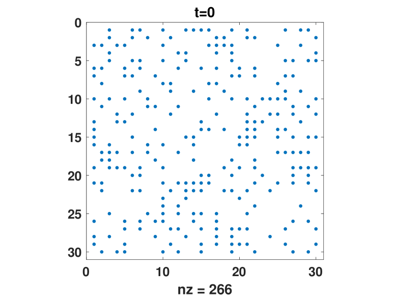
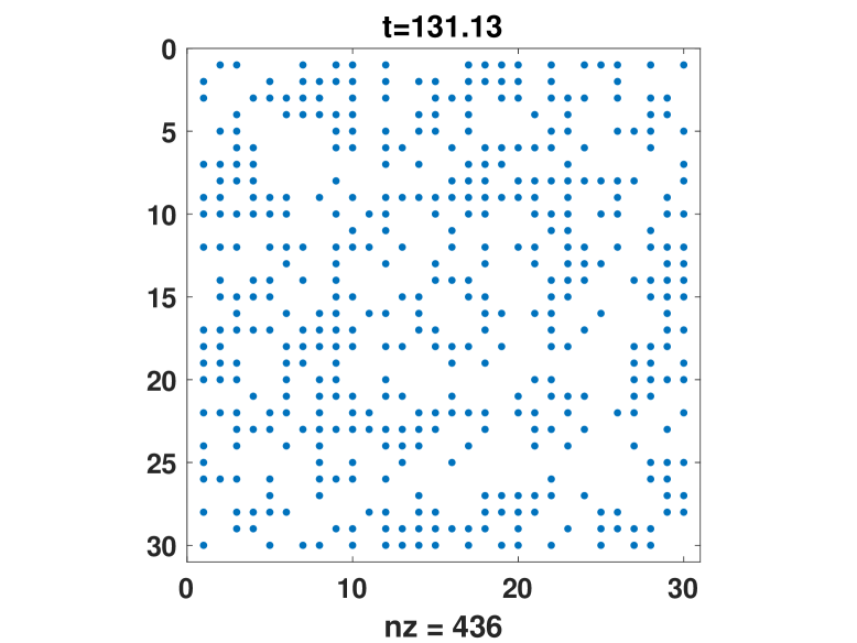
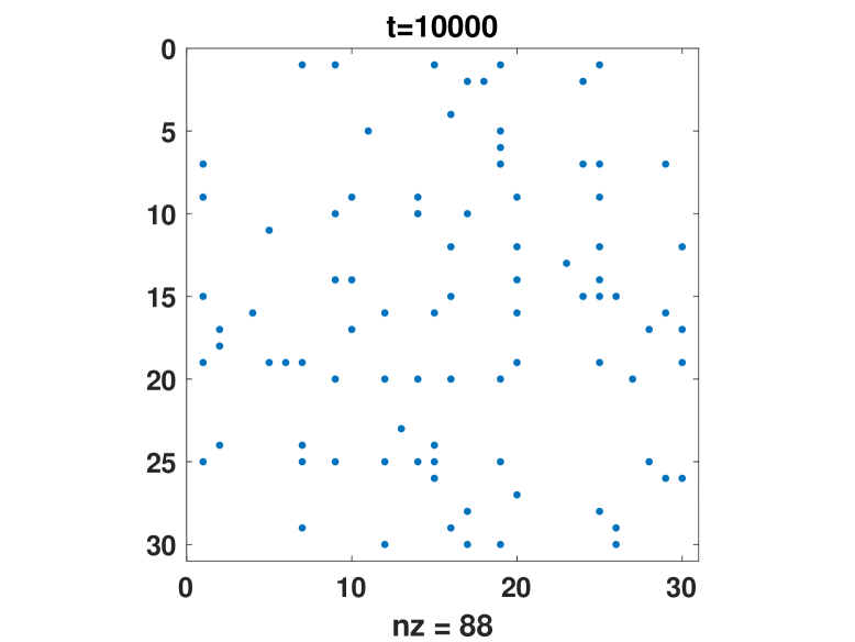
Figure 1: Time evolution of the adjacency matrix $A(t)$. Nonzeros are represented by dots. We show the connectivity at the initial time (upper left), at time of low density (upper right), a time of high density (lower left) and a later time where the density is again low (lower right). Here, we have $n=30$ nodes and nnz denotes the number of nonzeros in the adjacency matrix.

It is worth pointing out here that the elements of the adjacency matrix represent chemical species, and they can only take the value $0$ or $1$. However, given that there exist $N$ of them (using the fact that the adjacency matrix is symmetric) the Markov chain simulated by the algorithm described above has a state space of dimension $2^{N}$ (all the possible symmetric graphs with $n$-nodes). This in turn implies that as the number of nodes $n$ increases the computational cost of the algorithm will become a severe limiting factor in understanding the dynamics of the system. One possible way of accelerating the simulation is to use the $\tau$-leaping algorithm [17]. In the case $\tau=1$, this would essentially reduce to the model in [20].

We visualise in Figure 1 the adjacency matrix $A(t)$ at different time instances along a path computed by the SSA algorithm described above. Here a dot in the picture corresponds to the existence of an edge. We used reaction rate coefficients

$$c_{1}=0.025,\quad c_{2}=0.25,\quad c_{3}=0.91,$$ (9)

with $\widehat{c}_{3}$ defined in (4). Here, the initial configuration was a sample from the Erdős-Rényi class with parameter $p=0.3$, i.e., every edge has independent probability $p$ to exist at $t=0$. As $t$ increases the system is seen to transition between states of low and high connectivity. We can summarize the overall connectivity by the edge density

$$q(t):=\frac{1}{N}\sum_{i<j}\sum_{j}A(t)_{ij}.$$ (10)

In Figure 1, the upper and lower right states have edge density of around $0.18$ and $0.1$, respectively, and the lower left state has edge density of around $0.5$. The transitioning becomes clearer in Figure 2, where we plot the evolution of $q(t)$ for a range of different system sizes, again using an Erdős-Rényi initial condition with $p=0.3$. As $n$ is increased from $30$ to $50$, the edge density spends longer periods of time around each level. For $n=80$ and $n=100$, switching does not take place over the interval $0\leq t\leq 10^{4}$. We will return to these observations in the next section, where we construct and study an explanatory macroscopic approximation.

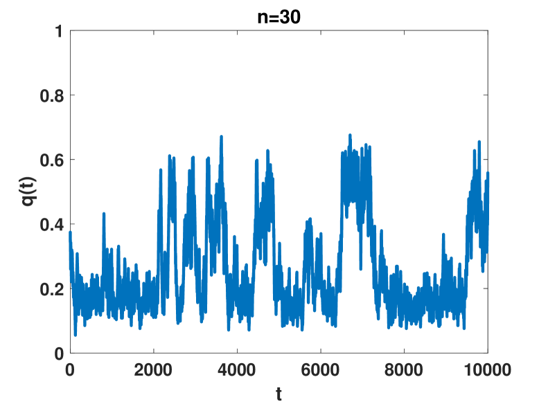
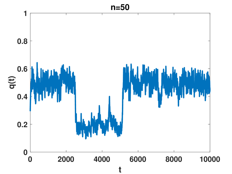
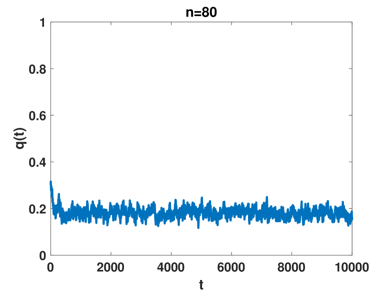
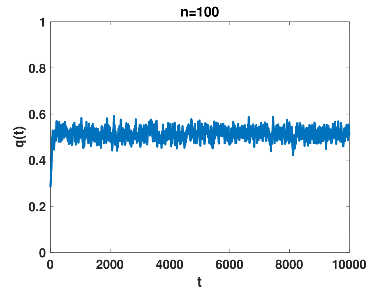
Figure 2: Evolution of edge density for $n=30,50,80,100$, up to time $t=10^{4}$.

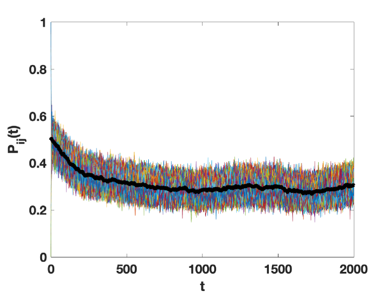
Figure 3: Time evolution of all $P_{ij}(t)$, the probability that the edge $i\leftrightarrow j$ exists at time $t$. Thick black line is the mean of $P_{ij}(t)$ over all $i$ and $j$.

Given that the overall edge density is a macroscopic quantity, it is natural to ask if it captures the effective behavior of the system. To investigate this issue, let $P_{ij}(t)$ denote the probability that the edge connecting $i$ and $j$ exists at time $t$. In Figure 3 we superimpose all the individual values $P_{ij}(t)$ for the case $n=30$. Here, we used a Monte Carlo approach to estimate each $P_{ij}(t)$ by applying SSA to compute $250$ independent paths. For each path, an initial state was chosen where half of the edges exist. We see that after a fast transient all probabilities fluctuate around a value that lies between the low and high edge density regimes that were seen in Figures 1 and 2. (The mean of $P_{ij}(t)$ over all $i$ and $j$ is superimposed as a thick black line.) This implies that after the initial transient the topology of the network is homogeneous in the sense that no nodes have distinguishable behavior.

3 Macroscopic Model

We saw in section 2 that after an initial transient the specific topology of the network appears to be homogeneous. Motivated by this observation we now define a simplified stochastic model. In this macroscopic model we do not retain any information about the topological structure of the network; we simply keep track of the number of edges. This reduces the size of the state space dramatically; in the microscopic model there are $2^{N}$ distinct networks. In this macroscopic model the scalar edge count ranges between $0$ and $N$. The simpler model allows long-time numerical simulation to be performed more efficiently, and, as we show in subsection 3.3, it is also amenable to rigorous analysis.

3.1 Macroscopic Regime

Our simplified, macroscopic version of the microscale system (1)–(3) involves two species: $E$ represents an edge and $O$ represents a missing edge. The species undergo three types of reaction, representing birth, death and triadic closure respectively:

$$O \rightarrow E,$$ (11)

$$E \rightarrow O,$$ (12)

$$O+E+E \rightarrow E+E+E.$$ (13)

The state vector may be written $X(t)\in\mathbb{R}^{2}$, where $X_{1}(t)$ and $X_{2}(t)$ record the number of edges (species $E$) and missing edges (species $O$), respectively. Notice that $X_{1}(t)+X_{2}(t)=N$ for all $t\geq 0$. The stoichiometric vectors for the three reactions are

$$\mbox{\boldmath$\nu$}_{1}=\left[\begin{array}[]{r}1\\ -1\end{array}\right],\quad\mbox{\boldmath$\nu$}_{2}=\left[\begin{array}[]{r}-1\\ 1\end{array}\right],\quad\mbox{\boldmath$\nu$}_{3}=\left[\begin{array}[]{r}1\\ -1\end{array}\right].$$

Reactions (11) and (12) are first order reactions that model spontaneous birth and death of edges. These effects are independent of the network structure, and hence we reproduce the corresponding birth and death behavior from the microscale model exactly by taking propensity functions $a_{1}(X(t))=c_{1}X_{2}(t)$, and $a_{2}(X(t))=c_{2}X_{1}(t)$, where $c_{1}$ and $c_{2}$ are the rate constants from (1) and (2). For the reaction (13) representing triadic closure, we must introduce simplifying assumptions, because the macroscale regime does not keep track of individual node and edge labels. Based on our observation in section 2, we suppose that at the current time $t$ edges are uniformly and independently distributed among the nodes—every possible edge $i\leftrightarrow j$ (with $i<j$) has a chance $X_{1}(t)/N$ of existing. (We note that this is effectively the mean field assumption used in [20].) Our aim is now to approximate the number of open wedges; that is, node triples $i,j,k$ such that edges $i\leftrightarrow j$ and $i\leftrightarrow k$ are present and edge $j\leftrightarrow k$ is absent. This quantity records the number of opportunities for the microscale reaction (3) to take place, and hence will be used in forming the propensity function at the macroscale level in (13).

To derive this approximation, we first note there are $X_{1}(t)$ ways to choose an edge $i\leftrightarrow j$. Then, fixing this $i$ and $j$, for every other node $k$ there is a chance of $\approx(X_{1}(t)-1)/N$ that the edge $i\leftrightarrow k$ also exists. So, taking into account all $n-2$ nodes, there are $\approx(n-2)X_{1}(t)(X_{1}(t)-1)/N$ chains of the form $j\leftrightarrow i\leftrightarrow k$. For any such chain, the chance of the third edge, $j\leftrightarrow k$, being absent is $\approx X_{2}(t)/N$. So the overall number of open wedges is $\approx(n-2)X_{1}(t)(X_{1}(t)-1)X_{2}(t)/N^{2}$. Hence, we find that a suitable propensity function for reaction (13) is

$$a_{3}(X(t))=\widehat{c}_{3}(n-2)X_{2}(t)X_{1}(t)(X_{1}(t)-1)/N^{2},$$ (14)

where $\widehat{c}_{3}$ is the rate constant in (3).

Since $X_{1}(t)+X_{2}(t)=N$, the macroscopic model (11)–(13) may be written as a scalar, continuous-time birth and death process for which $X_{1}(t)$ takes integer values between $0$ and $N$. Using $\lambda_{i}$ and $\mu_{i}$ to denote the overall birth and death rates, we have the general form

$$\mathbb{P}\left(X_{1}(t+\delta t)=i+1|X(t)=i\right) = \lambda_{i}\,\delta t+o(\delta t),\text{~{}for~{}}i=0,\ldots,N-1,$$ (15)

$$\mathbb{P}\left((X_{1}(t+\delta t)=i-1|X(t)=i\right) = \mu_{i}\,\delta t+o(\delta t),\text{~{}for~{}}i=1,\ldots,N.$$ (16)

Based on the arguments above, these birth and death rates take the form

$$\lambda_{i} = c_{1}(N-i)+\frac{\widehat{c}_{3}\,(n-2)}{N^{2}}(N-i)i(i-1),$$ (17)

$$\mu_{i} = c_{2}\,i.$$ (18)

Using the scaling (4), we obtain the birth rate

$$\lambda_{i}=N\left[c_{1}\left(1-\frac{i}{N}\right)+c_{3}\left(1-\frac{i}{N}\right)\left(\frac{i}{N}\right)\left(\frac{i-1}{N}\right)\right].$$ (19)

We then rewrite the death rate (18) as

$$\mu_{i}=Nc_{2}\,\frac{i}{N}.$$ (20)

We note in particular that the $\widehat{c}_{3}\propto 1/\sqrt{N}$ scaling from (4) has balanced the size of the separate terms in the birth and death rates (19) and (20).

We emphasize that $c_{1}$, $c_{2}$ and $c_{3}$ are regarded as positive constants and we have a family of birth and death processes parametrized by the system size, $N$, representing the number of edges.

3.2 Comparison between the Macroscopic and Microscopic Models

Having derived an approximation to the microscopic model in the previous subsection it is natural to compare individual paths of the two stochastic models. We will choose two sets of reaction constants $c_{1},c_{2},c_{3}$. From now on, and for reasons that will become apparent, we will refer to the parameters in (9) as the bistable regime, and we will also use a second set of parameters with a larger birth rate, $c_{1}$, given by

$$c_{1}=0.25,\quad c_{2}=0.25,\quad c_{3}=0.91.$$ (21)

We will refer to (21) as the monostable regime.

The behavior of paths in the monostable regime can be seen in the upper plots of Figure 4, for $n=30$ on the left and $n=100$ on the right. The initial state was an Erdős-Rényi sample with parameter $p=0.2$. For both values of $n$, we see that the microscopic and macroscopic models are behaving in the same way, namely having the edge density increasing towards a high value and oscillating around it. Additionally, we superimpose in these plots the solution of the deterministic mean field model in [20] (see also the discussion in Section 4). As we can see, both models agree closely with the mean field approximation, with the size of fluctuations becoming smaller for larger $n$.

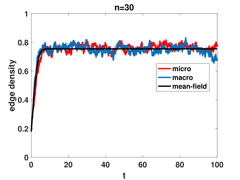
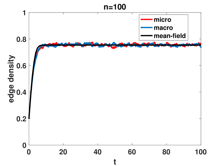
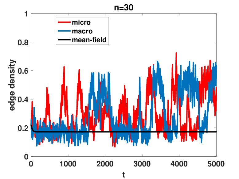
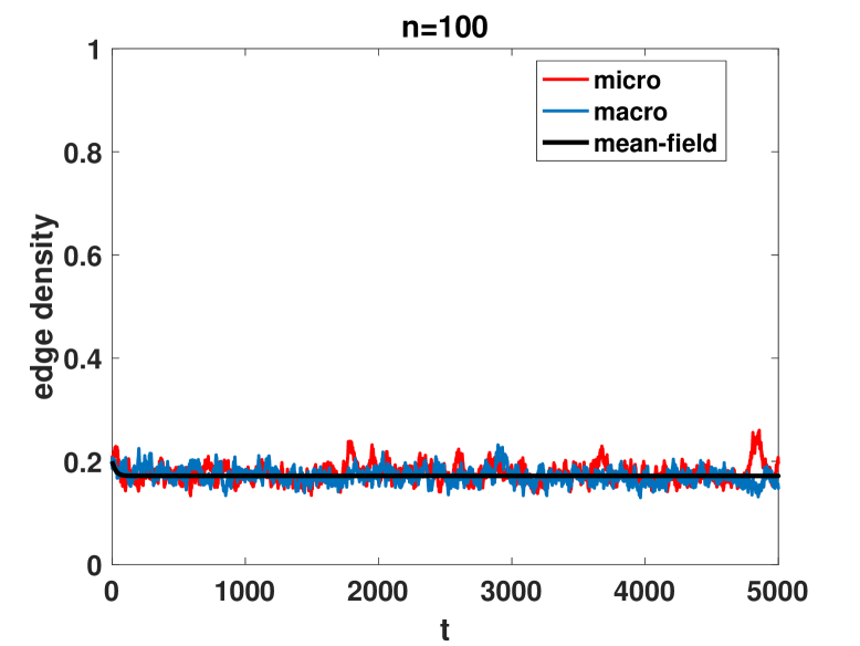
Figure 4: Comparison between the microscopic, the macroscopic and the mean field model. Erdős-Rényi initial configuration with $p=0.2$ using $n=30$ (left) and $n=100$ (right). Upper plots: monostable regime (21). Lower plots: bistable regime (9).

The behavior of the paths in the bistable parameter regime (9) can be seen in the lower plots of Figure 4. Again we have $n=30$ on the left and $n=100$ on the right and we used an Erdős-Rényi initial configuration with $p=0.2$. We see again there is excellent qualitative agreement between the microscopic and macroscopic paths. However, unlike the monostable regime, for $n=30$ the paths now do not agree with the mean field model, which, by its deterministic nature, does not switch between the low and high density regimes.

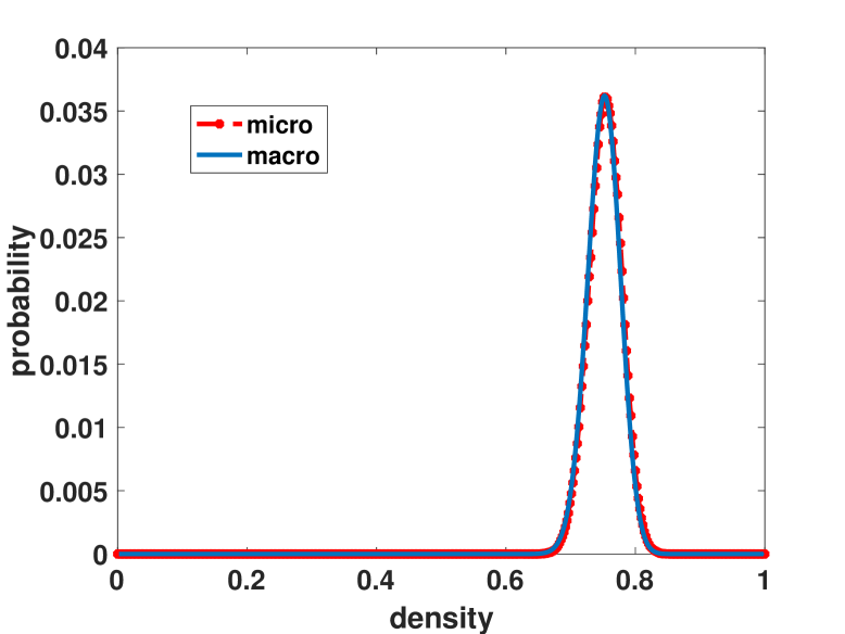
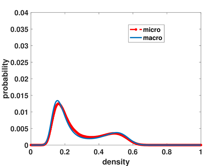
Figure 5: Comparison between the steady states of the microscopic and macroscopic models in the monostable (left, parameter set (21)) and bistable (right, parameter set (9)) regimes for $n=30$.

Our second comparison of the two models concerns their long time behavior. In the case of the macroscopic model, we will see in the next section that it is possible to obtain an analytic expression for the steady state. For the microscopic model it is not possible to derive an analytic expression for the steady state, so we used a long-time simulation ($T=5\times 10^{6}$ in the bistable case, $T=10^{4}$ in the monostable case). We plot this comparison in Figure 5. Here, the horizontal axis represents the scaled state values $0,1/N,2/N,\ldots,1$. We observe excellent agreement between the two steady states both in the monostable and bistable regime.

3.3 Steady State of Macroscopic Model

We now show that the bistable behavior observed in Figures 1 and 4 can be explained by analysing the long term behavior of the macroscopic model. Standard theory [30] shows that in our ergodic setting a process of the form (15)–(16) has a stationary distribution

$$\pi_{j}=\mathbb{P}\left(\lim_{t\to\infty}X_{1}(t)=j\right),\quad j=0,1,\ldots,N,$$

that satisfies

$$\pi_{j}=\displaystyle\frac{\prod_{i=0}^{j-1}\lambda_{i}}{\prod_{i=1}^{j}\mu_{j}}\pi_{0}.$$ (22)

In Figure 6 we show the steady state distribution in the bistable regime (9) when the number of nodes is $n=30$, $50$, $80$, and $100$. This figure may be compared with Figure 2. For internal consistency we have regarded these four curves as continuous-valued probability density functions over $[0,1]$, thereby normalizing them to have unit area. We see in Figure 6 that the bimodal steady state distribution has peaks at around $0.2$ and $0.5$, in agreement with the low and high connectivity regimes seen in Figure 2. We also see that although the location of the two peaks seems to be fixed, their relative heights vary. For $n=30$, the lower mode in Figure 6 captures more probability, which is consistent with the trajectory of $q(t)$ in Figure 2 spending more time in the lower connectivity regime. As $n$ increases the higher connectivity regime begins to dominate, and indeed the bimodality is barely visible for $n=100$ in Figure 6. This is consistent with the less frequent switching observed in Figure 2.

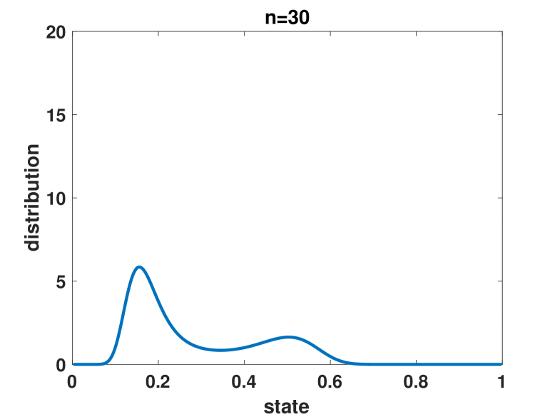
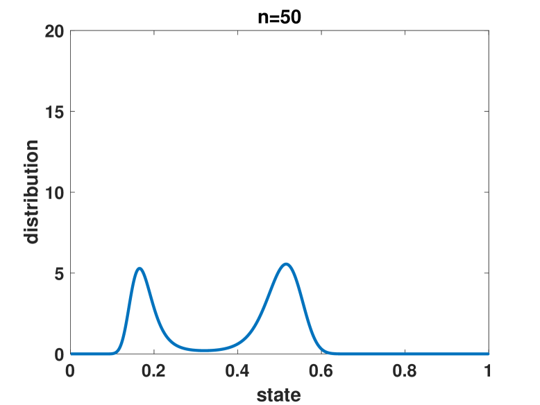
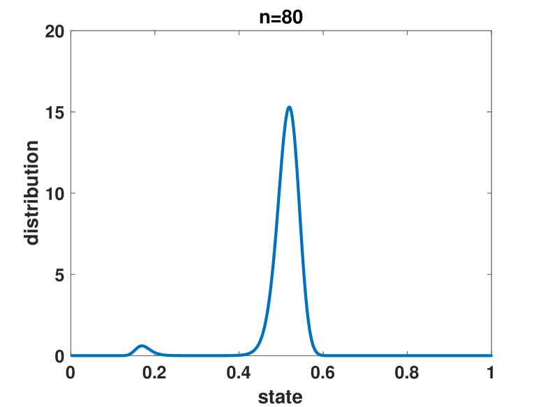
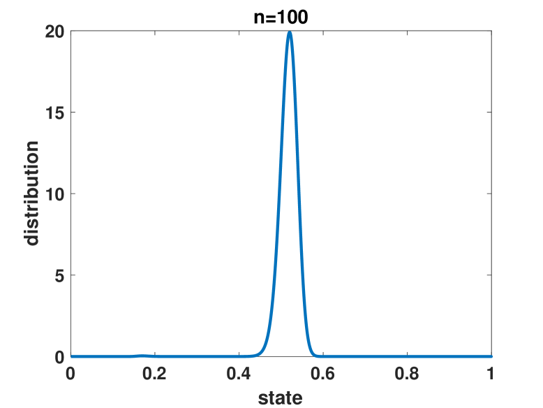
Figure 6: Steady state distribution of the macroscopic model (15)–(16) for $n=30,50,80,100$ in the bistable regime (9).

The following result shows that the bimodality of the macroscopic steady state is connected to the roots of the cubic equation (23), which depend only on $c_{1}$, $c_{2}$ and $c_{3}$. We note that these roots are $p_{1}^{\star}\approx 0.17$, $p_{2}^{\star}\approx 0.31$ and $p_{3}^{\star}\approx 0.52$ for the bistable regime used in Figures 2 and 6. (We also note that the cubic equation (23) has a single real root of $p^{\star}\approx 0.75$ in the monostable regime (21) used in the upper plots of Figure 4.)

Theorem 3.1.

Consider the scalar cubic equation

$$(1-p)(c_{1}+c_{3}p^{2})-c_{2}p=0,$$ (23)

for which any real root must necessarily lie in $(0,1)$. Then

(a)

the cubic equation has one real root $0<p^{\star}<1$ if and only if for sufficiently large $N$ the family of birth and death processes (15)–(16) with (19) and (20) has a unimodal steady state with maximum probability at state $j$, where $j/N=p^{\star}+O(1/N)$,

(b)

the cubic equation has three real roots $0<p_{1}^{\star}<p_{2}^{\star}<p_{3}^{\star}<1$ if and only if for sufficiently large $N$ the family of birth and death processes (15)–(16) with (19) and (20) has a bimodal steady state with locally maximum probability at state $j_{1}$, where $j_{1}/N=p_{1}^{\star}+O(1/N)$ and at state $j_{3}$, where $j_{3}/N=p_{3}^{\star}+O(1/N)$, and with locally minimum probability at state $j_{2}$ where $j_{2}/N=p_{2}^{\star}+O(1/N)$.

Proof.

Let

$$f(p)=\frac{(1-p)(c_{1}+c_{3}p^{2})}{c_{2}},$$ (24)

so a root of (23) corresponds to $f(p)=p$. Because $f(p)>0$ for $p<0$ and $f(p)<0$ for $p>1$, we see that any real root must lie in $(0,1)$. We know from (22) that $\pi_{j+1}/\pi_{j}=\lambda_{j}/\mu_{j+1}$. Hence, from (19), (20) and (24), we see that that for any $j=0,1,\ldots,N-1$,

$$\left|\frac{\pi_{j+1}}{\pi_{j}}-\frac{f(j/N)}{j/N}\right|\leq\frac{C}{N},$$ (25)

where $C$ is a constant that is uniform in $j$.

For case (a), suppose that the cubic has one root $p^{\star}$ in $(0,1)$. Then, by construction,

$$\frac{f(p)}{p}>1\text{~{}for~{}}p\in(0,p^{\star})\quad\text{and}\quad\frac{f(p)}{p}<1\text{~{}for~{}}p\in(p^{\star},1).$$

Let $j^{\star}$ be the largest $j$ such that $j/N\leq p^{\star}$. Then, for sufficiently large $N$, we see from (25) that

$$\frac{\pi_{j+1}}{\pi_{j}}>1\text{~{}for~{}}j<j^{\star}\quad\text{and}\quad\frac{\pi_{j+1}}{\pi_{j}}<1\text{~{}for~{}}j>j^{\star}.$$

Hence, $\pi_{0}<\pi_{1}<\cdots<\pi_{j^{\star}}$ and $\pi_{j^{\star}+1}>\pi_{j^{\star}+2}>\cdots>\pi_{N}$. So one or both of $\pi_{j^{\star}}$ and $\pi_{j^{\star}+1}$ give a maximum value.

On the other hand, suppose we have a unimodal distribution, that is, $\pi_{0}<\pi_{1}<\cdots<\pi_{j^{\star}}$ and $\pi_{j^{\star}+1}>\pi_{j^{\star}+2}>\cdots>\pi_{N}$. Then, by (25),

$$\frac{f(p)}{p}+O(1/N)>1\text{~{}for~{}}p=\frac{j}{N}\text{~{}with~{}}p<p^{\star}$$

and

$$\frac{f(p)}{p}+O(1/N)<1\text{~{}for~{}}p=\frac{j}{N}\text{~{}with~{}}p>p^{\star}.$$

For this to be true for all sufficiently large $N$, by continuity we must have a unique root in $(0,1)$ at $p^{\star}$.

Case (b) may be proved in a similar manner. ∎

3.4 Exit Times

Figures 2 and 6 suggest that for large $n$ there is a metastability effect, where the process spends a long time in a one regime before eventually switching to another. It is, of course, extremely challenging to verify such behavior by directly simulating a trajectory [5]. To gain further understanding of this type of behavior, we will study the expected time taken to move between modes in the bimodal case of the macroscopic model.

Let $G\in\mathbb{R}^{(N+1)\times(N+1)}$ be the tridiagonal matrix

$$\begin{bmatrix}-\lambda_{0}&\lambda_{0}&0&\dots&0\\ \\ \mu_{1}&-(\lambda_{1}+\mu_{1})&\lambda_{1}&\ddots&\vdots\\ \\ 0&\mu_{2}&-(\lambda_{2}+\mu_{2})&\lambda_{2}&\vdots\\ \\ \vdots&\ddots&\ddots&\ddots&\lambda_{N-1}\\ \\ 0&\dots&\dots&\mu_{N}&-\mu_{N}\end{bmatrix},$$ (26)

and, given $0\leq i\leq N$, let $Q^{[i]}\in\mathbb{R}^{N\times N}$ be the matrix obtained from $G$ by neglecting the $i$-th row and column, where we index from $0$ to $N$. Denote by $1_{N}$ the vector in $\mathbb{R}^{N}$ of all ones, and consider the linear system

$$Q^{[i]}\tau^{[i]}=-1_{N}.$$ (27)

The component $\tau^{[i]}_{j}$ then gives the mean time spent by the process (15)–(16) to reach the state $i$ starting from state $j$; that is,

$$\tau^{(i)}_{j}=\mathbb{E}\left[t:X(t)=i|X(0)=j\right],\quad j=0,\dots,N,\quad j\neq i.$$

Let $\lfloor\cdot\rfloor$ denote the integer flooring operation. In the case where the cubic (23) has three real roots, $0<p_{1}^{\star}<p_{2}^{\star}<p_{3}^{\star}$, and for a fixed value $n$, and hence $N$, we let $N_{1}=\lfloor p_{1}^{\star}N\rfloor$, $N_{2}=\lfloor p_{2}^{\star}N\rfloor$ and $N_{3}=\lfloor p_{3}^{\star}N\rfloor$. Hence, by Theorem 3.1, $N_{1}$ and $N_{3}$ are the state values corresponding to the peaks of the bimodal density, and $N_{2}$ corresponds to the trough in between. In Figure 7, on the left, by repeatedly solving appropriate systems of the form (27), we show the mean time taken for the process to move from $N_{1}$ to $N_{2}$ (dashed line) and from $N_{3}$ to $N_{2}$ (solid line), as a function of $n$. This characterizes for a specific system size $n$ how long it takes on average to switch between the two regimes. Note that both axes in Figure 7 are logarithmically scaled. We see that as the system size increases, the time to transition between the two modes increases dramatically. Moreover, for small $n$, the $N_{1}\to N_{2}$ transition takes longer than the $N_{3}\to N_{2}$ transition, whereas this relation changes over as $n$ increases. In Figure 7, on the right, we show the ratio of the $N_{1}\to N_{2}$ and $N_{3}\to N_{2}$ mean exit times. This behavior is consistent with the steady state plots in Figure 6, where for small (respectively, large) $n$ there is more probability mass around $N_{1}$ (respectively, $N_{3}$).

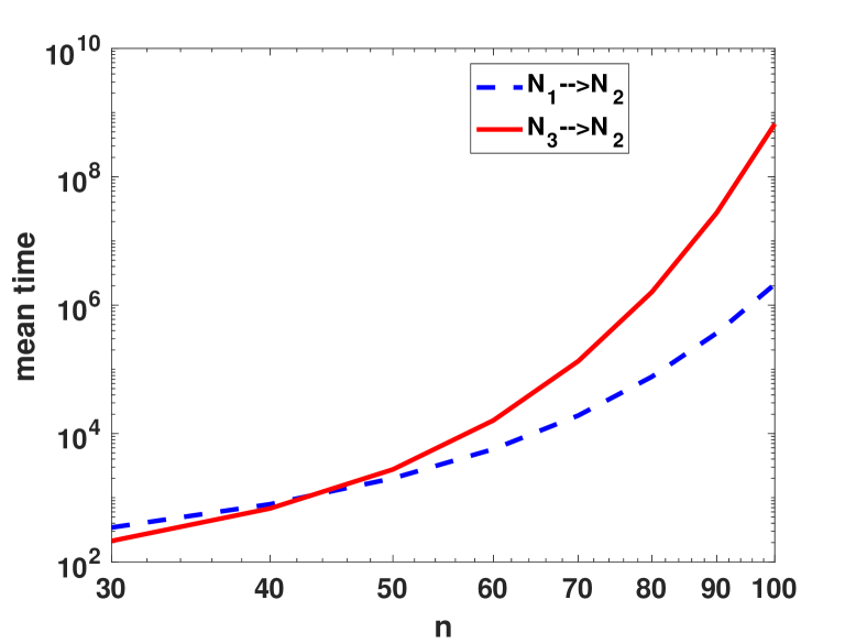
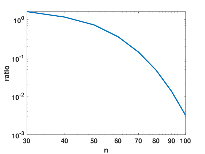
Figure 7: Bistable regime: mean time for the macroscale model to reach the central trough of the steady state, $N_{2}$, starting from each peak, $N_{1}$ and $N_{3}$ (left). Ratio between correspondent times (right).

4 Langevin and Deterministic ODE Models

The macroscale model (15)–(16) with (19) and (20) may be viewed as part of a hierarchy of models that includes a stochastic differential equation (SDE), or Langevin process, and a deterministic reaction rate ODE. We will first look at the Langevin version and test whether it retains the metastable behavior observed earlier.

Using standard arguments [15, 16] the Langevin equation may be written as an Ito SDE of the form

$$dy(t) = \mu(y(t))dt+\beta(y(t))d\mathbf{W}(t),$$ (28a)

$$\mu(y) = c_{1}\left(1-y\right)-c_{2}y+c_{3}(1-y)y^{2},$$ (28b)

$$\beta(y) = \frac{1}{\sqrt{N}}[\sqrt{c_{1}(1-y)},-\sqrt{c_{2}y},\sqrt{c_{3}(1-y)y^{2}}],$$ (28c)

where $\mathbf{W}(t)=[W_{1}(t),W_{2}(t),W_{3}(t)]^{T}$ is formed of three independent Brownian motions. Here the scalar, real-valued, random variable $y(t)$ represents the edge density at time $t$. Because of the presence of the square roots in (28c), the process becomes ill-defined when $y(t)$ leaves the interval $[0,1]$. This circumstance is common in Langevin formulations; intuitively, it arises from the fact that the approximations used to transfer between Poisson and diffusion processes break down when the molecule count for any species becomes small. Many approaches have been proposed to overcome this issue, see, for example, [1, 8, 26] and the references therein. We will avoid this difficulty by focusing on the mean first passage time for the SDE with a reflecting boundary at one end, thereby considering only paths that do not leave $[0,1]$. Letting

$$\sigma^{2}(y)=\frac{1}{N}\left(c_{1}\left(1-y\right)+c_{2}y+c_{3}(1-y)y^{2}\right),$$

we may then define the following partial differential operator

$$Lu:=\mu(y)\frac{du}{dy}+\frac{1}{2}\sigma^{2}(y)\frac{d^{2}u}{dy^{2}},$$ (29)

and the corresponding boundary value problem in the interval $(a,b)$

$$LT=-1,$$ (30)

subject to one of the two following pairs of boundary conditions:

$$T^{\prime}(0) = 0,\quad T(b)=0,$$ (31a)

$$T(a) = 0,\quad T^{\prime}(1)=0.$$ (31b)

The solution $T(x)$ with boundary conditions (31a) gives the mean time for paths of (28) starting from $x$ to reach the value $b$ when the SDE has a reflecting boundary condition at $y(t)=0$ [12]. Similarly, with the boundary conditions (31b), $T(x)$ gives the mean time for the SDE paths to reach $a$ starting from $x$ when there is a reflecting boundary condition at $y(t)=1$.

In the manner of Figure 7, in Figure 8 we show the mean times taken for the Langevin process to reach the central trough of the steady state distrubution (scaled to represent edge count rather than edge density) from each peak. The curves were obtained by numerically solving the relevant boundary value problems. Based on separate computations, not reported here, we believe that it is very unlikely for an SDE path to leave the interval $[0,1]$ over any reasonable timescale, and hence the reflecting boundary condition, which is introduced to avoid the technical issue of ill-defined square roots, has little effect on the results.

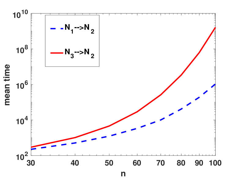
Figure 8: Analogues of the mean exit times in Figure 7 for the Langevin equation (28).

For further comparison, in Figure 9 we superimpose the mean exit times from Figure 7 (on the left) for the macroscale model and the mean first passage times from Figure 8 for the Langevin process. Here, we have plotted $n^{2}$ on the horizontal axis against the logarithm of the mean time on the vertical axis. We see that the SDE captures the extreme rate observed for the macroscale model, and for both models the mean time appears to scale like $\exp(n^{2})$, in line with the reaction rate theory of Kramers [21, 28]. It would, of course, be of interest to pursue the rigorous analysis of (28) with respect to long term behavior as the system size increases.

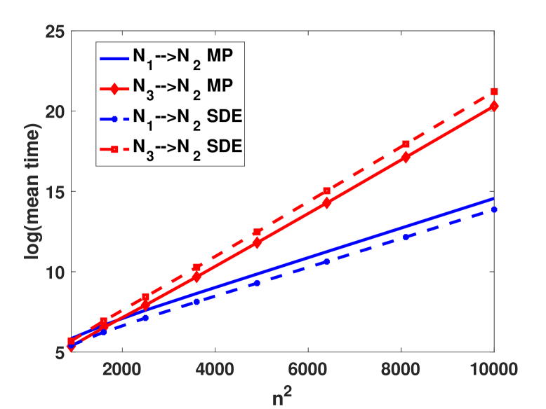
Figure 9: Comparison between mean exit times for the SDE (28) (as in Figure 8) and the macroscale Markov process (15)–(16) with (19) and (20) (as in Figure 7).

4.1 Deterministic Model

The reaction rate ODE arising from (28) takes the form $dy/dt=\mu(y(t))$. We note that $\mu$ coincides with the cubic in (23), and hence the edge densities $p^{\star}$ in part (a) of Theorem 3.1 and $p_{1}^{\star},p_{2}^{\star},p_{3}^{\star}$ in part (b) of Theorem 3.1 coincide with fixed points of this ODE. We also note that the deterministic mean field from [20] is essentially an Euler discretization of this ODE with unit stepsize. In the upper plots of Figure 4 we see that, in the monostable regime, the deterministic mean field approximation captures the long term behavior of the macro-level edge density. In the lower plots, corresponding to the bistable regime, the deterministic approximation is not able to switch, and hence settles on one of the two stable fixed points, $p_{1}^{\star}$ or $p_{3}^{\star}$, depending on the initial condition.

5 Discussion

Our aim in this work was to perform multiscale stochastic modeling and analysis to add insights to the bistability effect observed in [20]. A major objective was to develop simplified stochastic models that (a) reproduce the switching and metastability behavior observed for the full microscale model, (b) make long-term simulation feasible, and (c) offer the potential for rigorous analysis. A key step in this work was to set up a suitable scaling for the triadic closure reaction rate as a function of system size, i.e., the total number of possible edges, $N$. Returning to the original microscale model (1)–(3), we note that $\widehat{c}_{3}$ is the rate constant for each individual triadic closure reaction. So the chance of reaction (3) happening is $\widehat{c}_{3}$ if each of $O_{ij}$, $E_{jk}$ and $E_{ik}$ exist, and zero otherwise. Based on the way our macroscale approximations arose, it was then natural for $\widehat{c}_{3}$ to have the scaling $\widehat{c}_{3}\propto 1/\sqrt{N}$ in (4). Here, the chance of any individual triadic closure event taking place decreases as the system size grows. This scaling is necessary if we wish to be in a regime where spontaneous birth, spontaneous death and triadic closure all coexist for large system size. In particular, keeping $\widehat{c}_{3}$ constant as $N$ grows would lead to a system where triadic closure dominates, in general.

There are several directions in which this work could be pursued. For example, we note that although online social networking has the potential to increase the number of friendships an individual may form, there is evidence of an upper limit of around 150 in practice [4, 7]. This “Dunbar number” effect can be explained in part by cognitive constraints and in part by the time costs of maintaining relationships [6, 7]. In our model, in a bistable regime the low and high connectivity levels ($p_{1}^{\star}N$ and $p_{2}^{\star}N$ in Figure 6) lead to nodal degrees that become arbitrarily large in terms of $N$. Hence, in the case of very large networks it would be reasonable to investigate models that incorporate some sort of saturation or carrying capacity effect in order to limit the maximum number of friendships a person may maintain.

Furthermore, it is of course possible to move from triadic closure to more general mechanisms that encourage cliques [27] or other motifs to form in a network. Here new challenges include the incorporation of appropriate higher order matrix-level nonlinearities in expressions such as (7), and the justification of mean field approximations across longer-range interactions. Finally, it would be of interest to develop calibration methods along the lines of [25] in order to fit parameters to real data and search for bistability effects.

References

- [1] D. F. Anderson, D. J. Higham, S. C. Leite, and R. J. Williams, On constrained Langevin equations and (bio)chemical reaction networks, Multiscale Modeling and Simulation (SIAM), 17 (2019), pp. 1–30.
- [2] A. R. Benson, R. Abebe, M. T. Schaub, A. Jadbabaie, and J. Kleinberg, Simplicial closure and higher-order link prediction, Proceedings of the National Academy of Sciences, 115 (2018), pp. E11221–E11230.
- [3] A. R. Benson, D. F. Gleich, and J. Leskovec, Higher-order organization of complex networks, Science, 353 (2016), pp. 163–166.
- [4] J. Boase, J. B. Horrigan, B. Wellman, and L. Rainie, The strength of internet ties, in Pew Internet and American Life Project, 2006.
- [5] J. Carr, D. B. Duncan, and C. Walshaw, Numerical approximation of a metastable system, IMA Journal of Numerical Analysis, 15 (1995), pp. 505–521.
- [6] R. I. M. Dunbar, Neocortex size as a constraint on group size in primates, Journal of Human Evolution, 22 (1992), pp. 469–493.
- [7] , Do online social media cut through the constraints that limit the size of offline social networks?, R. Soc. Open Sci., 3 (2016), p. 3150292.
- [8] A. Duncan, R. Erban, and K. Zygalakis, Hybrid framework for the simulation of stochastic chemical kinetics, Journal of Computational Physics, 326 (2016), pp. 398–419.
- [9] D. Easley and J. Kleinberg, Networks, Crowds, and Markets: Reasoning About a Highly Connected World, Cambridge University Press, 2010.
- [10] E. Estrada and F. Arrigo, Predicting triadic closure in networks using communicability distance functions, SIAM Journal on Applied Mathematics, 75 (2015), pp. 1725–1744.
- [11] J. Fox, T. Roughgarden, C. Seshadhri, F. Wei, and N. Wein, Finding cliques in social networks: A new distribution-free model, SIAM J. Comput., 49 (2020), pp. 448–464.
- [12] C. W. Gardiner, Handbook of Stochastic Methods, for Physics, Chemistry and the Natural Sciences, Springer-Verlag, third ed., 2004.
- [13] D. T. Gillespie, A general method for numerically simulating the stochastic time evolution of coupled chemical reactions, J. Comp. Phys., 22 (1976), pp. 403—434.
- [14] , Exact stochastic simulation of coupled chemical reactions, J. Phys. Chem., 81 (1977), pp. 2340–2361.
- [15] D. T. Gillespie, Markov Processes: An Introduction for Physical Scientists, Academic Press, San Diego, 1991.
- [16] D. T. Gillespie, The chemical Langevin equation, J. Chem. Phys., 113 (2000), pp. 297–306.
- [17] , Approximate accelerated stochastic simulation of chemically reacting systems, Journal of Chemical Physics, 115 (2001), pp. 1716–1733.
- [18] M. S. Granovetter, The strength of weak ties, The American Journal of Sociology, 78 (1973), pp. 1360–1380.
- [19] P. Grindrod and D. J. Higham, Models for evolving networks: with applications in telecommunication and online activities, The IMA Journal of Management Mathematics, 23 (2012), pp. 1–16.
- [20] P. Grindrod, D. J. Higham, and M. C. Parsons, Bistability through triadic closure, Internet Math., 8 (2012), pp. 402–423.
- [21] P. Hänggi, P. Talkner, and M. Borkovec, Reaction-rate theory: fifty years after Kramers, Rev. Mod. Phys., 62 (1990), pp. 251–341.
- [22] J. Kim and J. Diesner, Over-time measurement of triadic closure in coauthorship networks, Social Network Analysis and Mining, 7 (2017).
- [23] T. G. Kolda, A. Pinar, T. Plantenga, C. Seshadhri, and C. Task, Counting triangles in massive graphs with MapReduce, SIAM Journal on Scientific Computing, 36 (2014), pp. S44–S77.
- [24] T. Lou, J. Tang, J. Hopcroft, Z. Fang, and X. Ding, Learning to predict reciprocity and triadic closure in social networks, ACM Trans. Knowl. Discov. Data, 7 (2013).
- [25] A. V. Mantzaris and D. J. Higham, Infering and calibrating triadic closure in a dynamic network, in Temporal Networks, P. Holme and J. Saramaki, eds., Springer, 2013, pp. 265–282.
- [26] M. Merritt, A. Alexanderian, and P. A. Gremaud, Multiscale global sensitivity analysis for stochastic chemical systems, Multiscale Modeling and Simulation (SIAM), (2021), pp. 440–459.
- [27] K. Pattiselanno, J. K. Dijkstra, C. Steglich, W. Vollebergh, and R. Veenstra, Structure matters: The role of clique hierarchy in the relationship between adolescent social status and aggression and prosociality, Journal of Youth and Adolescence, 44 (2015), pp. 2257–2274.
- [28] G. A. Pavliotis, Stochastic Processes and Applications: Diffusion Processes, the Fokker-Planck and Langevin Equations, Springer, Berlin, 2014.
- [29] G. Simmel, Soziologie: Untersuchungen über die Formen der Vergesellschaftung, Suhrkamp Verlag, Frankfurt, 1992 (Original work published in 1908).
- [30] H. M. Taylor and S. Karlin, An Introduction To Stochastic Modeling, Academic Press, San Diego, third edition ed., 1998.
- [31] L. Torres, A. Sizemore Blevins, D. S. Bassett, and T. Eliassi-Rad, The why, how, and when of representations for complex systems, SIAM Review, 63 (2021), pp. 435–485.
- [32] H. Yin, A. R. Benson, and J. Ugander, Measuring directed triadic closure with closure coefficients, Network Science, (2020), pp. 1–23.