Efficient Neural Network Training via
Forward and Backward Propagation Sparsification

Abstract

Sparse training is a natural idea to accelerate the training speed of deep neural networks and save the memory usage, especially since large modern neural networks are significantly over-parameterized. However, most of the existing methods cannot achieve this goal in practice because the chain rule based gradient (w.r.t. structure parameters) estimators adopted by previous methods require dense computation at least in the backward propagation step. This paper solves this problem by proposing an efficient sparse training method with completely sparse forward and backward passes. We first formulate the training process as a continuous minimization problem under global sparsity constraint. We then separate the optimization process into two steps, corresponding to weight update and structure parameter update. For the former step, we use the conventional chain rule, which can be sparse via exploiting the sparse structure. For the latter step, instead of using the chain rule based gradient estimators as in existing methods, we propose a variance reduced policy gradient estimator, which only requires two forward passes without backward propagation, thus achieving completely sparse training. We prove that the variance of our gradient estimator is bounded. Extensive experimental results on real-world datasets demonstrate that compared to previous methods, our algorithm is much more effective in accelerating the training process, up to an order of magnitude faster.

1 Introduction

In the last decade, deep neural networks (DNNs) [38, 13, 41] have proved their outstanding performance in various fields such as computer vision and natural language processing. However, training such large-sized networks is still very challenging, requiring huge computational power and storage. This hinders us from exploring larger networks, which are likely to have better performance. Moreover, it is a widely-recognized property that modern neural networks are significantly overparameterized, which means that a fully trained network can always be sparsified dramatically by network pruning techniques [12, 10, 27, 49, 22] into a small sub-network with negligible degradation in accuracy. After pruning, the inference efficiency can be greatly improved. Therefore, a natural question is can we exploit this sparsity to improve the training efficiency?

The emerging technique called sparse network training [11] is closely related with our question, which can obtain sparse networks by training from scratch. We can divide existing methods into two categories, i.e., parametric and non-parametric, based on whether they explicitly parameterize network structures with trainable variables (termed structure parameters). Empirical results [26, 37, 47, 25] demonstrate that the sparse networks they obtain have comparable accuracy with those obtained from network pruning. However, most of them narrowly aim at finding a sparse subnetwork instead of simultaneously sparsifying the computation of training by exploiting the sparse structure. As a consequence, it is hard for them to effectively accelerate the training process in practice on general platforms, e.g., Tensorflow [1] and Pytorch [33]. Detailed reasons are discussed below:

• Non-parametric methods find the sparse network by repeating a two-stage procedure that alternates between weight optimization and pruning [11, 8], or by adding a proper sparsity-inducing regularizer on the weights to the objective [24, 44]. The two-stage methods prune the networks in weight space and usually require retraining the obtained subnetwork from scratch every time when new weights are pruned, which makes training process even more time-consuming. Moreover, the computation of regularized methods is dense since the gradients of a zero-valued weights/filters are still nonzero.

• All the parametric approaches estimate the gradients based on chain rule. The gradient w.r.t. the structure parameters can be nonzero even when the corresponding channel/weight is pruned. Thus, to calculate the gradient via backward propagation, the error has to be propagated through all the neurons/channels. This means that the computation of backward propagation has to be dense. Concrete analysis can be found in Section 3.

We notice that some existing methods [5, 30] can achieve training speedup by careful implementation. For example, the dense to sparse algorithm [30] removes some channels if the corresponding weights are quite small for a long time. However, these methods always need to work with a large model at the beginning epochs and consume huge memory and heavy computation in the early stage. Therefore, even with such careful implementations, the speedups they can achieve are still limited.

In this paper, we propose an efficient channel-level parametric sparse neural network training method, which is comprised of completely sparse (See Remark 1) forward and backward propagation. We adopt channel-level sparsity since such sparsity can be efficiently implemented on the current training platforms to save the computational cost. In our method, we first parameterize the network structure by associating each filter with a binary mask modeled as an independent Bernoulli random variable, which can be continuously parameterized by the probability. Next, inspired by the recent work [50], we globally control the network size during the whole training process by controlling the sum of the Bernoulli distribution parameters. Thus, we can formulate the sparse network training problem into a constrained minimization problem on both the weights and structure parameters (i.e., the probability). The main novelty and contribution of this paper lies in our efficient training method called completely sparse neural network training for solving the minimization problem. Specifically, to fully exploit the sparse structure, we separate training iteration into two parts, i.e., weight update and structure parameter update. For weight update, the conventional backward propagation is used to calculate the gradient, which can be sparsified completely because the gradients of the filters with zero valued masks are also zero. For structure parameter update, we develop a new variance reduced policy gradient estimator (VR-PGE). Unlike the conventional chain rule based gradient estimators (e.g., straight through[3]), VR-PGE estimates the gradient via two forward propagations, which is completely sparse because of the sparse subnetwork. Finally, extensive empirical results demonstrate that our method can significantly accelerate the training process of neural networks.

The main contributions of this paper can be summarized as follows:

• We develop an efficient sparse neural network training algorithm with the following three appealing features:

  • In our algorithm, the computation in both forward and backward propagations is completely sparse, i.e., they do not need to go through any pruned channels, making the computational complexity significantly lower than that in standard training.

  • During the whole training procedure, our algorithm works on small sub-networks with the target sparsity instead of follows a dense-to-sparse scheme.

  • Our algorithm can be implemented easily on widely-used platforms, e.g., Pytorch and Tensorflow, to achieve practical speedup.

• We develop a variance reduced policy gradient estimator VR-PGE specifically for sparse neural network training, and prove that its variance is bounded.

• Experimental results demonstrate that our methods can achieve significant speed-up in training sparse neural networks. This implies that our method can enable us to explore larger-sized neural networks in the future.

Remark 1.

We call a sparse training algorithm completely sparse if both its forward and backward propagation do not need to go through any pruned channels. For such algorithms, the computational cost in forward and backward propagation cost can be roughly reduced to $\rho^{2}*100\%$, with $\rho$ being the ratio of remaining unpruned channels.

2 Related Work

In this section, we briefly review the studies on neural network pruning, which refers to the algorithms that prune DNNs after fully trained, and the recent works on sparse neural network training.

2.1 Neural Network Pruning

Network Pruning [11] is a promising technique for reducing the model size and inference time of DNNs. The key idea of existing methods [11, 10, 49, 22, 29, 15, 51, 43, 46, 35, 18] is to develop effective criteria (e.g, weight magnitude) to identify and remove the massive unimportant weights contained in networks after training. To achieve practical speedup on general devices, some of them prune networks in a structured manner, i.e., remove the weights in a certain group (e.g., filter) together, while others prune the weights individually. It has been reported in the literature [10, 27, 49, 22] that they can improve inference efficiency and reduce memory usage of DNNs by orders of magnitudes with minor loss in accuracy, which enables the deployment of DNNs on low-power devices.

We notice that although some pruning methods can be easily extended to train sparse networks, they cannot accelerate or could even slow down the training process. One reason is they are developed in the scenario that a fully trained dense network is given, and cannot work well on the models learned in the early stage of training. Another reason is after each pruning iteration, one has to fine tune or even retrain the network for lots of epoch to compensate the caused accuracy degradation.

2.2 Sparse Neural Network Training

The research on sparse neural network training has emerged in the recent years. Different from the pruning methods, they can find sparse networks without pre-training a dense one. Existing works can be divided into four categories based on their granularity in pruning and whether the network structures are explicitly parameterized. To the best of our knowledge, no significant training speedups achieved in practice are reported in the literature. Table 1 summarizes some representative works.

Table 1: Some representative works in sparse neural network training.

granularity	non-parametric	parametric
weight-level	[6, 8, 51, 24, 20, 31, 42, 32, 5]	[45, 40, 28, 50, 20]
channel-level	[44, 14]	[21, 26, 47, 28, 18]

Weight-level non-parametric methods, e.g., [8, 11, 51, 31, 32], always adopt a two-stage training procedure that alternates between weight optimization and pruning. They differ in the schedules of tuning the prune ratio over training and layers. [11] prunes the weights with the magnitude below a certain threshold and [51, 8] gradually increase the pruning rate during training. [32, 6] automatically reallocate parameters across layers during training via controlling the global sparsity.

Channel-level non-parametric methods [14, 44] are proposed to achieve a practical acceleration in inference. [44] is a structured sparse learning method, which adds a group Lasso regularization into the objective function of DNNs with each group comprised of the weights in a filter. [14] proposes a soft filter pruning method. It zeroizes instead of hard pruning the filters with small $\ell_{2}$ norm, after which these filters are treated the same with other filters in training. It is obvious that these methods cannot achieve significant speedup in training since they need to calculate the full gradient in backward propagation although the forward propagation could be sparsified if implemented carefully.

Parametric methods multiply each weight/channel with a binary [50, 47, 40, 45] or continuous [26, 28, 21, 20] mask, which can be either deterministic [26, 45] or stochastic [50, 47, 28, 40, 21, 20]. The mask is always parameterized via a continuous trainable variable, i.e., structure parameter. The sparsity is achieved by adding sparsity-inducing regularizers on the masks. The novelties of these methods lie in estimating the gradients w.r.t structure parameters in training. To be precise,

• Deterministic Binary Mask. [45] parameterizes its deterministic binary mask as a simple step function and estimates the gradients via sigmoid straight through estimator (STE) [3].

• Deterministic Continuous Mask. [26] uses the linear coefficients of batch normalization (BN) as a continuous mask and enforces most of them to 0 by penalizing the objective with $\ell_{1}$ norm of the coefficients. [20] defines the mask as a soft threshold function with learnable threshold. These methods can estimate the gradients via standard backward propagation.

• Stochastic Binary Mask. [47, 40] model the mask as a bernoulli random variable and the gradients w.r.t. the parameters of bernoulli distributions are estimated via STE. [50] estimates the gradients via Gumbel-Softmax trick [17], which is more accurate than STE.

• Stochastic Continuous Mask. [28, 21] parameterize the mask as a continuous function $g(c,\epsilon)$, which is differentiable w.r.t. $c$, and $\epsilon$ is a parameter free noise, e.g., Gaussian noise $\mathcal{N}(0,1)$. In this way, the gradients can be calcuated via conventional backward propagation.

Therefore, we can see that all of these parametric methods estimate the gradients of the structure parameters based on the chain rule in backward propagation. This makes the training iteration cannot be sparsified by exploiting the sparse network structure. For the details, please refer to Section 3.

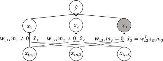
Figure 1: A fully connected network. $\boldsymbol{w}$ is the weight matrix of $1$st layer, $m_{i}$ is the mask of $i$-th neuron; $\hat{y}$, $\hat{\boldsymbol{x}}_{in}$ and $\hat{x}_{i}$ are the output, input and preactivation. The $3$rd neuron (in grey) is pruned.

3 Why Existing Parameteric Methods Cannot Achieve Practical Speedup?

In this section, we reformulate existing parametric channel-level methods into a unified framework to explain why they cannot accelerate the training process in practice.

Notice that convolutional layer can be viewed as a generalized fully connected layer, i.e., viewing the channels as neurons and convolution of two matrices as a generalized multiplication (see [9]). Hence, for simplicity, we consider the fully connected network in Figure 1. Moreover, since the channels in CNNs are corresponding to the neurons in fully connected networks, we consider neuron-level instead of weight-level sparse training in our example.

As discussed in Section 2, existing methods parameterize the 4 kinds of mask in the following ways:

$$\textup{(i): }m_{i}=\phi(s_{i});\quad \textup{(ii): }m_{i}=\psi(s_{i});\quad\textup{(iii): }m_{i}=g(s_{i},\epsilon),\epsilon\sim\mathcal{N}(0,1);\quad\textup{(iv): }m\sim\textup{Bern}(p_{i}(s)),$$

where the function $\phi(s_{i})$ is binary, e.g., step function; $\psi(s_{i})$ is a continuous function; $g(s_{i},\epsilon)$ is differentiable w.r.t. $s_{i}$. All existing methods estimate the gradient of the loss $\ell(\hat{y},y)$ w.r.t. $s_{i}$ based on chain rule, which can be formulated into a unified form below.

Specifically, we take the pruned neuron $x_{3}$ in Figure 1 as an example, the gradient is calculated as

$$\nabla_{s_{3}}\ell(\hat{y},y)=\underbrace{\frac{\partial{\ell(\hat{y},y)}}{\partial\hat{x}_{3}}}_{a}\underbrace{\left(\boldsymbol{w}^{\top}_{:,3}\boldsymbol{x}_{in}\right)}_{forward}\frac{\partial m_{3}}{\partial s_{3}}.$$ (1)

Existing parametric methods developed different ways to estimate $\frac{\partial m_{3}}{\partial s_{3}}$. Actually, for cases (ii) and (iii), the gradients are well-defined and thus can be calculated directly. STE is used to estimate the gradient in case (i) [45]. For cases (iv), [47, 40, 50] adopt STE and Gumbel-Softmax.

In Eqn.(1), the term (a) is always nonzero especially when $\hat{x}_{3}$ is followed by BN. Hence, we can see that even for the pruned neuron $x_{3}$, the gradient $\frac{\partial m_{3}}{\partial s_{3}}$ can be nonzero in all four cases. This means the backward propagation has to go though all the neurons/channels, leading to dense computation.

At last, we can know from Eqn.(1) that forward propagation in existing methods cannot be completely sparse. Although $\boldsymbol{w}^{\top}_{:,3}\boldsymbol{x}_{in}$ can be computed sparsely as in general models $\boldsymbol{x}_{in}$ could be a sparse tensor of a layer with some channels being pruned, we need to calculate it for each neuron via forward propagation to calculate RHS of Eqn.(1). Thus, even if carefully implemented, the computational cost of forward propagation can only be reduced to $\rho*100\%$ instead of $\rho^{2}*100\%$ as in inference.

That’s why we argue that existing methods need dense computation at least in backward propagation. So they cannot speed up the training process effectively in practice.

Remark 2.

The authors of GrowEfficient [47] confirmed that actually they also calculated the gradient of $q_{c}$ w.r.t, $\boldsymbol{s}_{c}$ in their Eqn.(6) via STE even if $q_{c}=0$. Thus need dense backward propagation.

4 Channel-level Completely Sparse Neural Network Training

Below, we present our sparse neural network training framework and the efficient training algorithm.

4.1 Framework of Channel-level Sparse Training

Given a convolutional network $f(x;\boldsymbol{w})$, let $\{\mathcal{F}_{c}:c\in\mathcal{C}\}$ be the set of filters with $\mathcal{C}$ being the set of indices of all the channels. To parameterize the network structure, we associate each $\mathcal{F}_{c}$ with a binary mask $m_{c}$, which is an independent Bernoulli random variable. Thus, each channel is computed as

$${\small\boldsymbol{x}_{\text{out, c}}=\boldsymbol{x}_{in}*\left(\mathcal{F}_{c}m_{c}\right),}$$

with $*$ being the convolution operation. Inspired by [50], to avoid the problems, e.g., gradient vanishing, we parameterize $m_{c}$ directly on the probability $s_{c}$, i.e., $m_{c}$ equals to 1 and 0 with the probabilities $s_{c}$ and $1-s_{c}$, respectively. Thus, we can control the channel size by the sum of $s_{c}$. Following [50], we can formulate channel-level sparse network training into the following framework:

$$\min_{\boldsymbol{w},\boldsymbol{s}}~{}\mathbb{E}_{p(\boldsymbol{m}|\boldsymbol{s})}~{}\mathcal{L}(\boldsymbol{w},\boldsymbol{m}):=\frac{1}{N}\sum_{i=1}^{N}\ell\left(f\left(\mathbf{x}_{i};\boldsymbol{w},\boldsymbol{m}\right),\mathbf{y}_{i}\right)$$ (2)

$$s.t.~{}\boldsymbol{w}\in\mathbb{R}^{n},\boldsymbol{s}\in\mathcal{S}:=\{\boldsymbol{s}\in[0,1]^{|\mathcal{C}|}:\boldsymbol{1}^{\top}\boldsymbol{s}\leq K\},$$

where $\left\{\left(\mathbf{x}_{i},\mathbf{y}_{i}\right)\right\}_{i=1}^{N}$ is the training dataset, $\boldsymbol{w}$ is the weights of the original network, $f\left(\cdot;\cdot,\cdot\right)$ is the pruned network, and $\ell(\cdot,\cdot)$ is the loss function, e.g, cross entropy loss. $K=\rho|\mathcal{C}|$ controls the remaining channel size with $\rho$ being the remaining ratio of the channels.

Discussion. We’d like to point out that although our framework is inspired by [50], our main contribution is the efficient solver comprised of completely sparse forward/backward propagation for Problem (2). Moreover, our framework can prune the weights in fully connected layers together, since we can associate each weight with an independent mask.

4.2 Completely Sparse Training with Variance Reduced Policy Gradient

Now we present our completely sparse training method, which can solve Problem (2) via completely sparse forward and backward propagation. The key idea is to separate the training iteration into filter update and structure parameter update so that the sparsity can be fully exploited.

4.2.1 Filter Update via Completely Sparse Computation

It is easy to see that the computation of the gradient w.r.t. the filters can be sparsified completely. To prove this point, we just need to clarify the following two things:

• We do not need to update the filters corresponding to the pruned channels. Consider a pruned channel $c$, i.e., $m_{c}=0$, then due to the chain rule, we can have

  $$\frac{\partial\ell\left(f\left(\mathbf{x}_{i};\boldsymbol{w},\boldsymbol{m}\right)\right)}{\partial\mathcal{F}_{c}}=\frac{\partial\ell\left(f\left(\mathbf{x}_{i};\boldsymbol{w},\boldsymbol{m}\right)\right)}{\partial\boldsymbol{x}_{out,c}}\frac{\partial\boldsymbol{x}_{out,c}}{\partial\mathcal{F}_{c}}\equiv 0,$$

  the last equation holds since $\boldsymbol{x}_{out,c}\equiv 0$. This indicates that the gradient w.r.t the pruned filter $\mathcal{F}_{c}$ is always 0, and thus $\mathcal{F}_{c}$ does not need to be updated.

• The error cannot pass the pruned channels via backward propagation. Consider a pruned channel $c$, we denote its output before masking as $\hat{\boldsymbol{x}}_{out,c}=\boldsymbol{x}_{in}*\mathcal{F}_{c}$, then the error propagating through this channel can be computed as

  $$\frac{\partial\ell\left(f\left(\mathbf{x}_{i};\boldsymbol{w},\boldsymbol{m}\right)\right)}{\partial\hat{\boldsymbol{x}}_{out,c}}=\frac{\partial\ell\left(f\left(\mathbf{x}_{i};\boldsymbol{w},\boldsymbol{m}\right)\right)}{\partial\boldsymbol{x}_{out,c}}\frac{\partial\boldsymbol{x}_{out,c}}{\hat{\boldsymbol{x}}_{out,c}}\equiv 0.$$

  This demonstrates that to calculate the gradient w.r.t. the unpruned filters, the backward propagation does not need to go through any pruned channels.

Therefore, the filters can be updated via completely sparse backward propagation.

4.2.2 Structure Parameter Update via Variance Reduced Policy Gradient

We notice that policy gradient estimator (PGE) can estimate the gradient via forward propagation, avoiding the pathology of chain rule based estimators as dicussed in Section 3. For abbreviation, we denote $\mathcal{L}(\boldsymbol{w},\boldsymbol{m})$ as $\mathcal{L}(\boldsymbol{m})$ since $\boldsymbol{w}$ can be viewed as a constant here. The objective can be written as

$$\Phi(\boldsymbol{s})=\mathbb{E}_{p(\boldsymbol{m}|\boldsymbol{s})}~{}\mathcal{L}(\boldsymbol{m}),$$

which can be optimized using gradient descent:

$$\boldsymbol{s}\leftarrow\boldsymbol{s}-\eta\nabla\Phi(\boldsymbol{s}).$$

with learning rate $\eta$. One can obtain a stochastic unbiased estimate of the gradient $\nabla\Phi(\boldsymbol{s})$ using PGE:

$$\nabla\Phi(\boldsymbol{s})=\mathbb{E}_{p(\boldsymbol{m}|\boldsymbol{s})}~{}\mathcal{L}(\boldsymbol{m})\nabla_{\boldsymbol{s}}\ln{p(\boldsymbol{m}|\boldsymbol{s})},$$ (PGE)

leading to Policy Gradient method, which may be regarded as a stochastic gradient descent algorithm:

$$\boldsymbol{s}\leftarrow\boldsymbol{s}-\eta\mathcal{L}(\boldsymbol{m})\nabla_{\boldsymbol{s}}\ln{p(\boldsymbol{m}|\boldsymbol{s})}.$$ (3)

In Eqn.(3), $\mathcal{L}(\boldsymbol{m})$ can be computed via completely sparse forward propagation and the computational cost of $\nabla_{\boldsymbol{s}}\ln{p(\boldsymbol{m}|\boldsymbol{s})}=\frac{\boldsymbol{m}-\boldsymbol{s}}{\boldsymbol{s}(1-\boldsymbol{s})}$ is negligible, therefore PGE is computationally efficient.

However, in accordance with the empirical results reported in [36, 17], we found that standard PGE suffers from high variance and does not work in practice. Below we will develop a Variance Reduced Policy Gradient Estimator (VR-PGE) starting from theoretically analyzing the variance of PGE.

Firstly, we know that this variance of PGE is

$$\mathbb{E}_{p(\boldsymbol{m}|\boldsymbol{s})}~{}\mathcal{L}^{2}(\boldsymbol{m})\|\nabla_{\boldsymbol{s}}\ln{p(\boldsymbol{m}|\boldsymbol{s})}\|_{2}^{2}-\|\nabla\Phi(\boldsymbol{s})\|_{2}^{2},$$

which can be large because $\mathcal{L}(\boldsymbol{m})$ is large.

Mean Field theory [39] indicates that, while $\mathcal{L}(\boldsymbol{m})$ can be large, the term $\mathcal{L}(\boldsymbol{m})-\mathcal{L}(\boldsymbol{m}^{\prime})$ is small when $\boldsymbol{m}$ and $\boldsymbol{m^{\prime}}$ are two independent masks sampled from a same distribution$p(\boldsymbol{m}|\boldsymbol{s})$ (see the appendix for the details). This means that we may consider the following variance reduced preconditioned policy gradient estimator:

$$\mathbb{E}_{\boldsymbol{m}^{\prime}\sim p(\boldsymbol{m}^{\prime}|\boldsymbol{s})}\mathbb{E}_{\boldsymbol{m}\sim p(\boldsymbol{m}|\boldsymbol{s})}~{}\left(\mathcal{L}(\boldsymbol{m})-\mathcal{L}(\boldsymbol{m}^{\prime})\right)H^{\alpha}(\boldsymbol{s})\nabla_{\boldsymbol{s}}\ln{p(\boldsymbol{m}|\boldsymbol{s})},$$ (VR-PGE)

where $H^{\alpha}(\boldsymbol{s})$ is a specific diagonal preconditioning matrix

$$H^{\alpha}(\boldsymbol{s})=\textup{diag}\left(\boldsymbol{s}\circ(1-\boldsymbol{s})\right)^{\alpha},$$ (4)

with $\alpha\in(0,1)$ and $\circ$ being the element-wise product. It plays a role as adaptive step size and it is shown that this term can reduce the variance of the stochastic PGE term $\nabla_{\boldsymbol{s}}\ln{p(\boldsymbol{m}|\boldsymbol{s})}$. The details can be found in the appendix. Thus $\Phi(\boldsymbol{s})$ can be optimized via:

$$\boldsymbol{s}\leftarrow\boldsymbol{s}-\eta\left(\mathcal{L}\left(\boldsymbol{m}\right)-\mathcal{L}\left(\boldsymbol{m}^{\prime}\right)\right)H^{\alpha}(\boldsymbol{s})\nabla_{\boldsymbol{s}}\ln{p(\boldsymbol{m}|\boldsymbol{s})}.$$ (5)

In our experiments, we set $\alpha$ to be $\frac{1}{2}$ for our estimator VR-PGE. The theorem below demonstrates that VR-PGE can have bounded variance.

Theorem 1.

Suppose $\boldsymbol{m}$ and $\boldsymbol{m^{\prime}}$ are two independent masks sampled from the Bernoulli distribution $p(\boldsymbol{m}|\boldsymbol{s})$, then for any $\alpha\in[\frac{1}{2},1)$ and $\boldsymbol{s}\in(0,1)^{|\mathcal{C}|}$, the variance is bounded for

$$\left(\mathcal{L}(\boldsymbol{m})-\mathcal{L}(\boldsymbol{m}^{\prime})\right)H^{\alpha}(\boldsymbol{s})\nabla_{\boldsymbol{s}}\ln{p(\boldsymbol{m}|\boldsymbol{s})}$$

Finally, we provide a complete view of our sparse training algorithm in Algorithm 1, which is essentially a projected stochastic gradient descent equipped with our efficient gradient estimators above. The projection operator in Algorithm 1 can be computed efficiently using Theorem 1 of [50].

Algorithm 1 Completely Sparse Neural Network Training

0: target remaining ratio $\rho$, a dense network $\boldsymbol{w}$, the step size $\eta$, and parameter $\alpha$ in (4) .

1: Initialize $\boldsymbol{w}$, let $\boldsymbol{s}=\rho\mathbf{1}$.

2: for training epoch $t=1,2\ldots T$ do

3:    for each training iteration do

4:       Sample mini batch of data $\mathcal{B}=\left\{\left(\mathbf{x}_{1},\mathbf{y}_{1}\right),\ldots,\left(\mathbf{x}_{B},\mathbf{y}_{B}\right)\right\}$.

5:       Sample $\boldsymbol{m}^{(i)}$ from $p(\boldsymbol{m}|\boldsymbol{s})$, $i=1,2$.

6:       Update $\boldsymbol{s}$ and $\boldsymbol{w}$ $\boldsymbol{s}\leftarrow\operatorname{proj}_{\mathcal{S}}(\boldsymbol{z})\mbox{ with }\boldsymbol{z}=\boldsymbol{s}-\eta\left(\mathcal{L}_{\mathcal{B}}(\boldsymbol{w},\boldsymbol{m}^{(1)})-\mathcal{L}_{\mathcal{B}}(\boldsymbol{w},\boldsymbol{m}^{(2)})\right)H^{\alpha}(\boldsymbol{s})\frac{\boldsymbol{m}^{(1)}-\boldsymbol{s}}{\boldsymbol{s}(1-\boldsymbol{s})},$$\boldsymbol{w}\leftarrow\boldsymbol{w}-\eta\nabla_{\boldsymbol{w}}\mathcal{L}_{\mathcal{B}}\left(\boldsymbol{w},\boldsymbol{m}^{(1)}\right)$

7:    end for

8: end for

9: return  A pruned network $\boldsymbol{w}\circ\boldsymbol{m}$ by sampling a mask $\boldsymbol{m}$ from the distribution $p(\boldsymbol{m}|\boldsymbol{s})$.

Discussion. In our algorithm, benefited from our constraint on $\boldsymbol{s}$, the channel size of the neural network during training can be strictly controlled. This is in contrast with GrowEfficient [47], which ultilizes regularizer term to control the model size and has situations where model size largely drift away from desired. This will have larger demand for the GPU memory storage and have more risk that memory usage may explode, especially when we utilize sparse learning to explore larger models. Moreover, our forward and backward propagations are completely sparse, i.e., they do not need to go through any pruned channels. Therefore, the computational cost of each training iteration can be roughly reduced to $\rho^{2}*100\%$ of the dense network.

5 Experiments

In this section, we conduct a series of experiments to demonstrate the outstanding performance of our method. We divide the experiments into five parts. In part one, we compare our method with several state-of-the-art methods on CIFAR-10 [19] using VGG-16 [38], ResNet-20 [13] and WideResNet-28-10 [48] to directly showcase the superiority of our method. In part two, we directly compare with state-of-the-art method GrowEfficient [47] especially on extremely sparse regions, and on two high capacity networks VGG-19 [38] and ResNet-32 [13] on CIFAR-10/100 [19]. In part three, we conduct experiments on a large-scale dataset ImageNet [4] with ResNet-50 [13] and MobileNetV1 [16] and compare with GrowEfficient [47] across a wide sparsity region. In part four, we present the train-computational time as a supplementary to the conceptual train-cost savings to justify the applicability of sparse training method into practice. In part five, we present further analysis on epoch-wise train-cost dynamics and experimental justification of variance reduction of VR-PGE. Due to the space limitation, we postpone the experimental configurations, calculation schemes on train-cost savings and train-computational time and additional experiments into appendix.

5.1 VGG-16, ResNet-20 and WideResNet-28-10 on CIFAR-10

Table 2: Comparison with the channel pruning methods L1-Pruning [22], SoftNet [14], ThiNet [29], Provable [23] and one channel sparse training method GrowEfficient [47] on CIFAR-10.

Model	Method	Val Acc(%)	Params(%)	FLOPs(%)	Train-Cost Savings($\times$)
VGG-16	Original	92.9	100	100	1$\times$
	L1-Pruning	91.8	19.9	19.9	-
	SoftNet	92.1	36.0	36.1	-
	ThiNet	90.8	36.0	36.1	-
	Provable	92.4	5.7	15.0	-
	GrowEfficient	92.5	5.0	13.6	1.22$\times$
	Ours	92.5	4.4	8.7	8.69$\times$
ResNet-20	Original	91.3	100	100	1$\times$
	L1-Pruning	90.9	55.6	55.4	-
	SoftNet	90.8	53.6	50.6	-
	ThiNet	89.2	67.1	67.3	-
	Provable	90.8	37.3	54.5	-
	GrowEfficient	90.91	35.8	50.2	1.13$\times$
	Ours	90.93	35.1	36.1	2.09$\times$
WRN-28-10	Original	96.2	100	100	1$\times$
	L1-Pruning	95.2	20.8	49.5	-
	GrowEfficient	95.3	9.3	28.3	1.17$\times$
	Ours	95.6	8.4	7.9	9.39$\times$

Table 2 presents Top-1 validation accuracy, parameters, FLOPs and train-cost savings comparisons with channel pruning methods L1-Pruning [22], SoftNet [14], ThiNet [29], Provable [23] and sparse training method GrowEfficient [47]. SoftNet can train from scratch but requires completely dense computation. Other pruning methods all require pretraining of dense model and multiple rounds of pruning and finetuning, which makes them slower than vanilla dense model training. Therefore the train-cost savings of these methods are below 1$\times$ and thus shown as ("-") in Table 2.

GrowEfficient [47] is a recently proposed state-of-the-art channel-level sparse training method showing train-cost savings compared with dense training. As described in Section 3, GrowEfficient features completely dense backward and partially sparse forward pass, making its train-cost saving limited by $\frac{3}{2}$. By contrast, the train-cost savings of our method is not limited by any constraint. The details of how train-cost savings are computed can be found in appendix.

Table 2 shows that our method generally exhibits better performance in terms of validation accuracy, parameters and particularly FLOPs. In terms of train-cost savings, our method shows at least 1.85$\times$ speed-up against GrowEfficient [47] and up to 9.39$\times$ speed-up against dense training.

5.2 Wider Range of Sparsity on CIFAR-10/100 on VGG-19 and ResNet-32

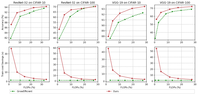
Figure 2: Comparison of Top-1 Validation Accuracy and Train-cost Savings on CIFAR-10/100.

In this section, we explore sparser regions of training efficiency to present a broader comparision with state-of-the-art channel sparse training method GrowEfficient [47].

We plot eight figures demonstrating the relationships between the Top-1 validation accuracy, FLOPs and train-cost savings. We find that our method generally achieves higher accuracy under same FLOPs settings. To be noted, the train-cost savings of our method is drastically higher than GrowEfficient [47], reaching up to 58.8$\times$ when sparisty approches 1.56% on ResNet-32 on CIFAR-100, while the speed-up of GrowEfficient is limited by $\frac{3}{2}$.

Table 3: Comparison with the channel pruning methods L1-Pruning [22], SoftNet [14], Provable [23] and one channel sparse training method GrowEfficient [47] on ImageNet-1K.

Model	Method	Val Acc(%)	Params(%)	FLOPs(%)	Train-Cost Savings($\times$)
ResNet-50	Original	77.0	100	100	1$\times$
	L1-Pruning	74.7	85.2	77.5	-
	SoftNet	74.6	-	58.2	-
	Provable	75.2	65.9	70.0	-
	GrowEfficient	75.2	61.2	50.3	1.10$\times$
	Ours	76.0	48.2	46.8	1.60$\times$
	Ours	73.5	27.0	24.7	3.02$\times$
	Ours	69.3	10.8	10.1	7.36$\times$

5.3 ResNet-50 and MobileNetV1 on ImageNet-1K

In this section, we present the performance boost obtained by our method on ResNet-50 and MobileNetV1 on ImageNet-1K [4]. Our method searches a model with 76.0% Top-1 accuracy, 48.2% parameters and 46.8% FLOPs beating all compared state-of-the-art methods. The train-cost saving comes up to 1.60$\times$ and is not prominent due to the accuracy constraint to match up with compared methods. Therefore we give a harder limit to the channel size and present sparser results on the same Table 3, reaching up to 7.36$\times$ speed-up while still preserving 69.3% Top-1 accuracy. For the already compact model MobileNetV1, we plot two figures in Figure 3 comparing with GrowEfficient [47]. We find that our method is much stabler in sparse regions and obtains much higher train-cost savings.

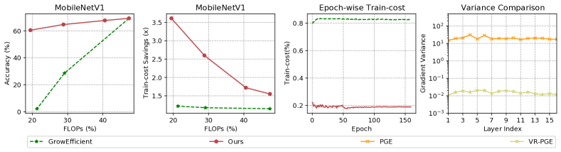
Figure 3: Top-1 Validation Accuracy and Train-cost Savings on MobileNetV1 on ImageNet. Epoch-wise Train-cost and Variance Comparison on VGG-19 on CIFAR-10.

5.4 Actual Training Computational Time Testing

In this section, we provide actual training computational time on VGG-19 and CIFAR-10. The GPU in test is RTX 2080 Ti and the deep learning framework is Pytorch [33]. The intent of this section is to justify the feasibility of our method in reducing actual computational time cost, rather than staying in conceptual training FLOPs reduction. The computational time cost is measured by wall clock time, focusing on forward and backward propagation. We present training computational time in Table 4 with varying sparsity as in Figure 2. It shows that the computational time savings increases steadily with the sparisty. We also notice the gap between the savings in FLOPS and computational time. The gap comes from the difference between FLOPs and actual forward/backward time. More specifically, forward/backward time is slowed down by data-loading processes and generally affected by hardware latency and throughput, network architecture, etc. At extremely sparse regions, the pure computational time of sparse networks only occupies little of the forward/backward time and the cost of data management and hardware latency dominates the wall-clock time. Despite this gap, it can be expected that our train-cost savings can be better translated into real speed-up in exploring large models where the pure computational time dominates the forward/backward time, which promises a bright future for making training infeasibly large models into practice.

Table 4: Train-computational Time on VGG-19 with CIFAR-10. The computational time saving is not as prominent as train-cost savings while still achieving nearly an order of reduction, preserving 87.97% accuracy.

Model	Val Acc(%)	Params(%)	FLOPs(%)	Train-Cost Savings($\times$)	Train-Computational Time(min)
VGG-19	93.84	100.00	100.00	1.00$\times$	21.85 (1.00$\times$)
	93.46	23.71	28.57	2.64$\times$	14.04 (1.55$\times$)
	93.11	12.75	19.33	3.89$\times$	10.43 (2.09$\times$)
	92.23	6.69	10.27	7.30$\times$	6.83 (3.20$\times$)
	90.82	3.06	4.94	15.28$\times$	4.86 (4.50$\times$)
	87.97	0.80	1.70	44.68$\times$	2.95 (7.41$\times$)

5.5 Further Analysis

[Epoch-wise Train-cost Dynamics of Sparse Training Process] We plot the train-cost dynamics in Figure 3. The vertical label is the ratio of train-cost to dense training, the inverse of train-cost savings. This demonstrates huge difference between our method and GrowEfficient [47]. The model searched by our method exhibits 92.73% Top-1 accuracy, 16.68% parameters, 14.28% FLOPs with 5.28$\times$ train-cost savings, while the model searched by GrowEfficient exhibits 92.47% Top-1 accuracy, 18.08% parameters, 22.74% FLOPs with 1.21$\times$ train-cost savings.

[Experimental Verification of Variance Reduction of VR-PGE against PGE] We plot the mean of variance of gradients of channels from different layers. The model checkpoint and input data are selected randomly. The gradients are calculated in two approaches, VR-PGE and PGE. From the rightmost graph of Figure 3, we find that the VR-PGE reduces variance significantly, up to 3 orders of magnitude.

6 Conclusion

This paper proposes an efficient sparse neural network training method with completely sparse forward and backward passes. A novel gradient estimator named VR-PGE is developed for updating structure parameters, which estimates the gradient via two sparse forward propagation. We theoretically proved that VR-PGE has bounded variance. In this way, we can separate the weight and structure update in training and making the whole training process completely sparse. Emprical results demonstrate that the proposed method can significantly accelerate the training process of DNNs in practice. This enables us to explore larger-sized neural networks in the future.

Appendix A Proof of Theorem 1

A.1 Properties of Overparameterized Deep Neural Networks

Before giving the detailed proof, we would like to present the following two properties of overparameterized deep neural networks, which are implied by the latest studies based on the mean field theory. We will empirically verify these properties in this section and adopt them as assumptions in our proof.

Property 1.

Given the probability $\boldsymbol{s}$ and the weights $\boldsymbol{w}$ for an overparameterized deep neural network, then for two independent masks $\boldsymbol{m}$ and $\boldsymbol{m}^{\prime}$ sampled from $p(\cdot|\boldsymbol{s})$, $\mathcal{L}(\boldsymbol{m})-\mathcal{L}(\boldsymbol{m}^{\prime})$ is always small. That is

$$V(\boldsymbol{s}):=\mathbb{E}_{\boldsymbol{m}\sim p(\cdot|\boldsymbol{s})}\mathbb{E}_{\boldsymbol{m}^{\prime}\sim p(\cdot|\boldsymbol{s})}\left(\mathcal{L}(\boldsymbol{m})-\mathcal{L}(\boldsymbol{m}^{\prime})\right)^{2}$$ (6)

is small.

The mean field theory based studies [39, 7] proved that discrete deep neural networks can be viewed as sampling neurons/channels from continuous networks according to certain distributions. As the numbers of neurons/channels increase, the output of discrete networks would converge to that of the continuous networks (see Theorem 3 in [39] and Theorem 1 in [7]). Although in standard neural networks we do not have the scaling operator as [39, 7] for computing the expectation, due to the batch normalization layer, the affect caused by this difference can largely be eliminated. The subnetworks $\boldsymbol{m}$ and $\boldsymbol{m}^{\prime}$ here can be roughly viewed as sampled from a common continuous network. Therefore, $\mathcal{L}(\boldsymbol{m})-\mathcal{L}(\boldsymbol{m}^{\prime})$ would be always small. That’s why Property 1 holds.

Property 2.

Given the probability $\boldsymbol{s}$ and the weights $\boldsymbol{w}$ for an overparameterized deep neural network, consider a mask $\boldsymbol{m}$ sampled from $p(\cdot|\boldsymbol{s})$, if we flip one component of $\boldsymbol{m}$, then the network would not change too much. Combined with Property 1, this can be stated as: for any $j\in\mathcal{C}$, we denote $\boldsymbol{m}_{-j}$ and $\boldsymbol{s}_{-j}$ to be all the components of $\boldsymbol{m}$ and $\boldsymbol{s}$ except the $j$-th component, and define

$$V_{\max}(\boldsymbol{s}):=\max_{\boldsymbol{m}_{j}\in\{0,1\},j\in\mathcal{C}}\mathbb{E}_{\boldsymbol{m}_{-j}\sim p(\cdot|\boldsymbol{s}_{-j})}\mathbb{E}_{\boldsymbol{m}^{\prime}\sim p(\cdot|\boldsymbol{s})}\left(\mathcal{L}(\boldsymbol{m})-\mathcal{L}(\boldsymbol{m}^{\prime})\right)^{2},$$

then

$$V_{\max}(\boldsymbol{s})\approx V(\boldsymbol{s}).$$ (7)

In the mean field based studies [39, 7], they model output of a neuron/channel as a expectation of weighted sum of the neurons/channels in the previous layer w.r.t. a certain distribution. Therefore, the affect of flipping one component of the mask on expectation is negligible. Therefore Property 2 holds.

A.2 Detailed Proof

Proof.

In this proof, we denote

$$\left(\mathcal{L}(\boldsymbol{m})-\mathcal{L}(\boldsymbol{m}^{\prime})\right)H^{\alpha}(\boldsymbol{s})\nabla_{\boldsymbol{s}}\ln{p(\boldsymbol{m}|\boldsymbol{s})}$$

as $\mathcal{G}^{\alpha}(\boldsymbol{m},\boldsymbol{m}^{\prime}|\boldsymbol{s})$. Note that the total variance

$$\mbox{Var}(\mathcal{G}^{\alpha}(\boldsymbol{m},\boldsymbol{m}^{\prime}|\boldsymbol{s}))$$

$$= \mathbb{E}_{\boldsymbol{m}\sim p(\cdot|\boldsymbol{s})}\mathbb{E}_{\boldsymbol{m}^{\prime}\sim p(\cdot|\boldsymbol{s})}\|\mathcal{G}^{\alpha}(\boldsymbol{m},\boldsymbol{m}^{\prime}|\boldsymbol{s})\|_{2}^{2}-\|\mathbb{E}_{\boldsymbol{m}\sim p(\cdot|\boldsymbol{s})}\mathbb{E}_{\boldsymbol{m}^{\prime}\sim p(\cdot|\boldsymbol{s})}\mathcal{G}^{\alpha}(\boldsymbol{m},\boldsymbol{m}^{\prime}|\boldsymbol{s})\|_{2}^{2},$$

we only need to prove that the term $\mathbb{E}_{\boldsymbol{m}\sim p(\cdot|\boldsymbol{s})}\mathbb{E}_{\boldsymbol{m}^{\prime}\sim p(\cdot|\boldsymbol{s})}\|\mathcal{G}^{\alpha}(\boldsymbol{m},\boldsymbol{m}^{\prime}|\boldsymbol{s})\|_{2}^{2}$ is bounded.

We let $\boldsymbol{m}_{-j}$ and $\boldsymbol{s}_{-j}$ be all the components of $\boldsymbol{m}$ and $\boldsymbol{s}$ except the $j$-th component with $j\in\mathcal{C}$. We consider the $j$-th component of $\mathcal{G}^{\alpha}(\boldsymbol{m},\boldsymbol{m}^{\prime}|\boldsymbol{s})$, i.e., $\mathcal{G}_{j}^{\alpha}(\boldsymbol{m},\boldsymbol{m}^{\prime}|\boldsymbol{s})$, then $\mathbb{E}_{\boldsymbol{m}\sim p(\cdot|\boldsymbol{s})}\mathbb{E}_{\boldsymbol{m}^{\prime}\sim p(\cdot|\boldsymbol{s})}\|\mathcal{G}_{j}^{\alpha}(\boldsymbol{m},\boldsymbol{m}^{\prime}|\boldsymbol{s})\|_{2}^{2}$ can be estimated as

$$\mathbb{E}_{\boldsymbol{m}\sim p(\cdot|\boldsymbol{s})}\mathbb{E}_{\boldsymbol{m}^{\prime}\sim p(\cdot|\boldsymbol{s})}\left(\mathcal{G}_{j}^{\alpha}(\boldsymbol{m},\boldsymbol{m}^{\prime}|\boldsymbol{s})\right)^{2}$$

$$= \mathbb{E}_{\boldsymbol{m}\sim p(\cdot|\boldsymbol{s})}\mathbb{E}_{\boldsymbol{m}^{\prime}\sim p(\cdot|\boldsymbol{s})}\left(\mathcal{L}(\boldsymbol{m})-\mathcal{L}(\boldsymbol{m}^{\prime})\right)^{2}[H^{\alpha}(\boldsymbol{s})\nabla_{\boldsymbol{s}}\ln{p(\boldsymbol{m}|\boldsymbol{s})}]_{j}^{2}$$

$$= \mathbb{E}_{\boldsymbol{m}\sim p(\cdot|\boldsymbol{s})}\mathbb{E}_{\boldsymbol{m}^{\prime}\sim p(\cdot|\boldsymbol{s})}\left(\mathcal{L}(\boldsymbol{m})-\mathcal{L}(\boldsymbol{m}^{\prime})\right)^{2}\left(\boldsymbol{s}_{j}^{2\alpha}(1-\boldsymbol{s}_{j})^{2\alpha}\frac{(\boldsymbol{m}_{j}-\boldsymbol{s}_{j})^{2}}{\boldsymbol{s}^{2}_{j}(1-\boldsymbol{s}_{j})^{2}}\right)$$ (8)

$$= \mathbb{E}_{\boldsymbol{m}\sim p(\cdot|\boldsymbol{s})}\mathbb{E}_{\boldsymbol{m}^{\prime}\sim p(\cdot|\boldsymbol{s})}\left(\mathcal{L}(\boldsymbol{m})-\mathcal{L}(\boldsymbol{m}^{\prime})\right)^{2}\left(\boldsymbol{s}_{j}^{2(\alpha-1)}(1-\boldsymbol{s}_{j})^{2(\alpha-1)}(\boldsymbol{m}_{j}-\boldsymbol{s}_{j})^{2}\right)$$

$$= \mathbb{E}_{\boldsymbol{m}_{j}\sim p(\cdot|\boldsymbol{s}_{j})}\left(\mathbb{E}_{\boldsymbol{m}_{-j}\sim p(\cdot|\boldsymbol{s}_{-j})}\mathbb{E}_{\boldsymbol{m}^{\prime}\sim p(\cdot|\boldsymbol{s})}\left(\mathcal{L}(\boldsymbol{m})-\mathcal{L}(\boldsymbol{m}^{\prime})\right)^{2}\right)\left(\boldsymbol{s}_{j}^{2(\alpha-1)}(1-\boldsymbol{s}_{j})^{2(\alpha-1)}(\boldsymbol{m}_{j}-\boldsymbol{s}_{j})^{2}\right)$$

$$\mathop{\leq}_{\eqref{eqn:property-flip}} V_{\max}(\boldsymbol{s})\mathbb{E}_{\boldsymbol{m}_{j}\sim p(\cdot|\boldsymbol{s}_{j})}\left(\boldsymbol{s}_{j}^{2(\alpha-1)}(1-\boldsymbol{s}_{j})^{2(\alpha-1)}(\boldsymbol{m}_{j}-\boldsymbol{s}_{j})^{2}\right)$$ (9)

$$= \left(\boldsymbol{s}_{j}^{2\alpha}(1-\boldsymbol{s}_{j})^{(2\alpha-1)}+\boldsymbol{s}_{j}^{2\alpha-1}(1-\boldsymbol{s}_{j})^{2\alpha}\right)V_{\max}(\boldsymbol{s}).$$ (10)

Thus $\mathbb{E}_{\boldsymbol{m}\sim p(\cdot|\boldsymbol{s})}\mathbb{E}_{\boldsymbol{m}^{\prime}\sim p(\cdot|\boldsymbol{s})}\|\mathcal{G}^{\alpha}(\boldsymbol{m},\boldsymbol{m}^{\prime}|\boldsymbol{s})\|_{2}^{2}$ can be estimated as follows:

$$\mathbb{E}_{\boldsymbol{m}\sim p(\cdot|\boldsymbol{s})}\mathbb{E}_{\boldsymbol{m}^{\prime}\sim p(\cdot|\boldsymbol{s})}\|\mathcal{G}^{\alpha}(\boldsymbol{m},\boldsymbol{m}^{\prime}|\boldsymbol{s})\|_{2}^{2}$$

$$= \sum_{j\in\mathcal{C}}\mathbb{E}_{\boldsymbol{m}\sim p(\cdot|\boldsymbol{s})}\mathbb{E}_{\boldsymbol{m}^{\prime}\sim p(\cdot|\boldsymbol{s})}\left(\mathcal{G}_{j}^{\alpha}(\boldsymbol{m},\boldsymbol{m}^{\prime}|\boldsymbol{s})\right)^{2}$$

$$\leq V_{\max}(\boldsymbol{s})\sum_{j\in\mathcal{C}}\boldsymbol{s}_{j}^{2\alpha}(1-\boldsymbol{s}_{j})^{(2\alpha-1)}+\boldsymbol{s}_{j}^{2\alpha-1}(1-\boldsymbol{s}_{j})^{2\alpha}.$$ (11)

Thus, when $\alpha\in[\frac{1}{2},1)$, we have

$$\mathbb{E}_{\boldsymbol{m}\sim p(\cdot|\boldsymbol{s})}\mathbb{E}_{\boldsymbol{m}^{\prime}\sim p(\cdot|\boldsymbol{s})}\|\mathcal{G}^{\alpha}(\boldsymbol{m},\boldsymbol{m}^{\prime}|\boldsymbol{s})\|_{2}^{2}$$

$$\leq V_{\max}(\boldsymbol{s})\sum_{j\in\mathcal{C}}\boldsymbol{s}_{j}^{2\alpha}(1-\boldsymbol{s}_{j})^{(2\alpha-1)}+\boldsymbol{s}_{j}^{2\alpha-1}(1-\boldsymbol{s}_{j})^{2\alpha}$$

$$\leq |\mathcal{C}|V_{\max}(\boldsymbol{s}).$$

The last inequality holds since the term $\boldsymbol{s}_{j}^{2\alpha}(1-\boldsymbol{s}_{j})^{(2\alpha-1)}+\boldsymbol{s}_{j}^{2\alpha-1}(1-\boldsymbol{s}_{j})^{2\alpha}$ is monotonically decreasing w.r.t. $\alpha\in[\frac{1}{2},1)$.

Therefore, from Property 1 and 2, we can see that the variance is bounded for any $\boldsymbol{s}$.

∎

Remark 3.

Eqn. (8) and (9) indicate that $H^{\alpha}(\boldsymbol{\boldsymbol{s}})$ is introduced to reduce the variance of the stochastic PGE term $\nabla_{\boldsymbol{s}}\ln{p(\boldsymbol{m}|\boldsymbol{s})}$. Without $H^{\alpha}(\boldsymbol{\boldsymbol{s}})$ (i.e., $\alpha=0$), from Eqn.(11), we can see that the total variance bound would be

$$V_{\max}(\boldsymbol{s})\sum_{j\in\mathcal{C}}\frac{1}{(1-\boldsymbol{s}_{j})}+\frac{1}{\boldsymbol{s}_{j}}.$$

Because of the sparsity constraints, lots of $\boldsymbol{s}_{j}$ would be close to $0$. Hence, the total variance in this case could be very large.

Remark 4.

Our preconditioning matrix $H^{\alpha}(\boldsymbol{s})$ plays a role as adaptive step size. The hyper-parameter $\alpha$ can be used to tune its effect on variance reduction. For a large variance $\nabla_{\boldsymbol{s}}\ln{p(\boldsymbol{m}|\boldsymbol{s})}$ we can use a large $\alpha$. In our experiments, we find that simply letting $\alpha=\frac{1}{2}$ works well.

A.3 Convergence of Our Method

For the weight update, the convergence can be guaranteed since we use the standard stochastic gradient descent with the gradient calculated via backward propagation.

For the parameter $\boldsymbol{s}$, as stated in Section 4.2.2, we update it as:

$$\boldsymbol{s}\leftarrow\boldsymbol{s}-\eta\left(\mathcal{L}\left(\boldsymbol{m}\right)-\mathcal{L}\left(\boldsymbol{m}^{\prime}\right)\right)H^{\alpha}(\boldsymbol{s})\nabla_{\boldsymbol{s}}\ln{p(\boldsymbol{m}|\boldsymbol{s})}.$$ (12)

Let $\Delta\boldsymbol{s}(\boldsymbol{m},\boldsymbol{m}^{\prime}|\boldsymbol{s})$ be $\left(\mathcal{L}\left(\boldsymbol{m}\right)-\mathcal{L}\left(\boldsymbol{m}^{\prime}\right)\right)H^{\alpha}(\boldsymbol{s})\nabla_{\boldsymbol{s}}\ln{p(\boldsymbol{m}|\boldsymbol{s})}$, we can have

$$\mathbb{E}_{\boldsymbol{m}\sim p(\cdot|\boldsymbol{s})}\mathbb{E}_{\boldsymbol{m}^{\prime}\sim p(\cdot|\boldsymbol{s})}\Delta\boldsymbol{s}(\boldsymbol{m},\boldsymbol{m}^{\prime}|\boldsymbol{s})$$

$$= \mathbb{E}_{\boldsymbol{m}\sim p(\cdot|\boldsymbol{s})}\mathbb{E}_{\boldsymbol{m}^{\prime}\sim p(\cdot|\boldsymbol{s})}\left(\mathcal{L}\left(\boldsymbol{m}\right)-\mathcal{L}\left(\boldsymbol{m}^{\prime}\right)\right)H^{\alpha}(\boldsymbol{s})\nabla_{\boldsymbol{s}}\ln{p(\boldsymbol{m}|\boldsymbol{s})}$$

$$= \mathbb{E}_{\boldsymbol{m}\sim p(\cdot|\boldsymbol{s})}\mathcal{L}\left(\boldsymbol{m}\right)H^{\alpha}(\boldsymbol{s})\nabla_{\boldsymbol{s}}\ln{p(\boldsymbol{m}|\boldsymbol{s})}-\mathbb{E}_{\boldsymbol{m}\sim p(\cdot|\boldsymbol{s})}\mathbb{E}_{\boldsymbol{m}^{\prime}\sim p(\cdot|\boldsymbol{s})}\mathcal{L}\left(\boldsymbol{m}^{\prime}\right)H^{\alpha}(\boldsymbol{s})\nabla_{\boldsymbol{s}}\ln{p(\boldsymbol{m}|\boldsymbol{s})}$$

$$= H^{\alpha}(\boldsymbol{s})\mathbb{E}_{\boldsymbol{m}\sim p(\cdot|\boldsymbol{s})}\mathcal{L}\left(\boldsymbol{m}\right)\nabla_{\boldsymbol{s}}\ln{p(\boldsymbol{m}|\boldsymbol{s})}-H^{\alpha}(\boldsymbol{s})\mathbb{E}_{\boldsymbol{m}^{\prime}\sim p(\cdot|\boldsymbol{s})}\mathcal{L}\left(\boldsymbol{m}^{\prime}\right)\underbrace{\mathbb{E}_{\boldsymbol{m}\sim p(\cdot|\boldsymbol{s})}\nabla_{\boldsymbol{s}}\ln{p(\boldsymbol{m}|\boldsymbol{s})}}_{I}$$

$$= H^{\alpha}(\boldsymbol{s})\mathbb{E}_{\boldsymbol{m}\sim p(\cdot|\boldsymbol{s})}\mathcal{L}\left(\boldsymbol{m}\right)\nabla_{\boldsymbol{s}}\ln{p(\boldsymbol{m}|\boldsymbol{s})}$$ (13)

$$= H^{\alpha}(\boldsymbol{s})\nabla_{\boldsymbol{s}}\mathbb{E}_{\boldsymbol{m}\sim p(\cdot|\boldsymbol{s})}\mathcal{L}\left(\boldsymbol{m}\right),$$

where Eqn.(13) holds since term $I=\nabla_{\boldsymbol{s}}\mathbb{E}_{\boldsymbol{m}\sim p(\cdot|\boldsymbol{s})}\boldsymbol{1}\equiv 0$.

Therefore, we can see that $\Delta\boldsymbol{s}(\boldsymbol{m},\boldsymbol{m}^{\prime}|\boldsymbol{s})$ is an unbiased gradient estimator associated with an adaptive step size, i.e., our VR-PGE is a standard preconditioned stochastic gradient descent method. Thus, the convergence can be guaranteed.

A.4 Experiments Verfiying Properties 1 and 2 in A.1

Figure 4 presents the values of $\mathbb{E}_{\boldsymbol{m}\sim p(\cdot|\boldsymbol{s})}\mathcal{L}^{2}(\boldsymbol{m})$, $V(\boldsymbol{s})$ and $V_{\max}(\boldsymbol{s})$ during the training process of ResNet-32 on CIFAR-10. We can see that $V(\boldsymbol{s})$ and $V_{\max}(\boldsymbol{s})$ are very close during the whole training process and they are smaller than $\mathbb{E}_{\boldsymbol{m}\sim p(\cdot|\boldsymbol{s})}\mathcal{L}^{2}(\boldsymbol{m})$ by four orders of magnitude. This verifies our Property 1 and 2.

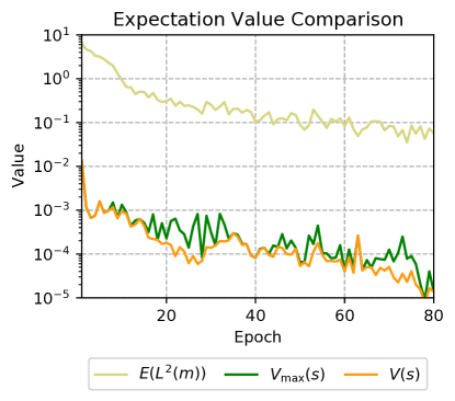
Figure 4: Experiments on ResNet32 on CIFAR-10. $V(\boldsymbol{s})$ and $V_{\max}(\boldsymbol{s})$ are very close during the whole training process and they are smaller than $\mathbb{E}_{\boldsymbol{m}\sim p(\cdot|\boldsymbol{s})}\mathcal{L}^{2}(\boldsymbol{m})$ by four orders of magnitude.

Appendix B Experimental Configurations

[CIFAR-10/100 Experiments] GPUs: 1 for VGG and ResNet and 2 for WideResNet. Batch Size: 256. Weight Optimizer: SGD. Weight Learning Rate: 0.1. Weight Momentum: 0.9. Probability Optimizer: Adam. Probability Learning Rate: 12e-3. WarmUp: ✗. Label Smoothing: ✗.

[ImageNet-1K Experiments] GPUs: 4. Batch Size: 256. Weight Optimizer: SGD. Weight Learning Rate: 0.256. Weight Momentum: 0.875. Probability Optimizer: Adam. Probability Learning Rate: 12e-3. WarmUp: ✓. Label Smoothing: 0.1.

Remark 5.

The bold-face probability learning rate 12e-3 is the only hyperparameter obtained by grid search on CIFAR-10 experiments and applied directly to larger datasets and networks. Other hyperparameters are applied following the same practice of previous works [34, 20, 27, 51]. The channels of ResNet32 for CIFAR experiments are doubled following the same practice of [42].

Table 5: Forward/backward time of dense/sparse networks and accompanying properties.

Model	Val Acc(%)	Params(%)	Forward(min)	Backward(min)	Train-Computational Time(min)
VGG-19	93.84	100.00	6.89	14.96	21.85 (1.00$\times$)
	93.46	23.71	6.41	7.63	14.04 (1.55$\times$)
	93.11	12.75	4.89	5.54	10.43 (2.09$\times$)
	92.23	6.69	3.10	3.73	6.83 (3.20$\times$)
	90.82	3.06	2.15	2.71	4.86 (4.50$\times$)
	87.97	0.80	1.27	1.68	2.95 (7.41$\times$)

Appendix C Calculation Schemes on Train-cost Savings and Train-computational Time

C.1 Train-cost Savings

The train-cost of vanilla dense training can be computed as two parts: in forward propagation, calculating the loss of weights and in backward propagation, calculating the gradient of weights and gradient of the activations of the previous layers. The FLOPs of backward propagation is about 2$\sim$3 times of forward propagation [2]. In the following calculation, we calculate the FLOPs of forward propagation concretely and consider FLOPs of backward propagation 2 times of forward propagation for simplicity.

[GrowEfficient] The forward propagation of dense network is $f_{D}$. The forward propagation of GrowEfficient is partially sparse with FLOPs being $f_{S}$ and backward propagation is dense. Therefore the train-cost saving is computed as $\frac{f_{D}+2f_{D}}{f_{S}+f_{D}}=\frac{3}{2+f_{S}/f_{D}}$, upper-bounded by $\frac{3}{2}$.

[Ours] The forward propagation of dense network is $f_{D}$. The forward propagation and backward propagation is totally sparse. The FLOPs of forward propagation is $f_{S}$ and the FLOPs of backward propagation is $2*f_{S}$. The forward propagation has to be computed two times. Therefore the train-cost saving is computed as $\frac{f_{D}+2*f_{D}}{2*f_{S}+2*f_{S}}=\frac{3}{4f_{S}/f_{D}}$. Actually, $f_{S}/f_{D}$ is roughly equal to $\rho^{2}$, leading to drastically higher train-cost savings.

C.2 Train-computational Time

The calculation of train-computational time focuses on the forward and backward propagation of dense/sparse networks. For both of the dense and sparse networks, we sum up the computation time of all the forward and backward propagation in the training process as the train-computational time. The detailed time cost is presented in Table 5. We can see that we can achieve significant speedups in computational time.

Appendix D Potentials and Limitations of This Work

[On Computational Cost Saving] Although our method needs two forward propagation in each iteration, we have to point out that our method can achieve significant computational cost saving. The reason is that our forward and backward is completely sparse, whose computational complexity is roughly $\rho^{2}*100\%$ of the conventional training algorithms with $\rho$ being the remain ratio of the channels.

[On Exploring Larger Networks] About the potential of our method in exploring larger networks, we’d like to clarify the following three things:

• The memory cost of the structure parameters $\boldsymbol{s}$ is negligible compared with the original weight $\boldsymbol{w}$ as each filter is associated with only one structure parameter, therefore our $\boldsymbol{s}$ would hardly increase the total memory usage.

• Although in our method, we need to store the parameter of the full model, this would not hinder us from exploring larger networks. The reason is that, in each iteration, we essentially perform forward and backward propagation on the sparse subnetwork. More importantly, we find that reducing the frequency of sampling subnetwork, e.g., sample a new subnetwork for every 50 iterations, during training would not affect the final accuracy. In this way, we can store the parameters of the full model on CPU memory and store the current subnetwork on GPU, and synchronize the parameters’ updates to the full model only when we need to resample a new subnetwork. Hence, our method has great potentials in exploring larger deep neural networks. We left such engineering implements as the future work and we also welcome the engineers in the community to implement our method more efficiently.

• In exploring larger networks, the channel remain ratio $\rho$ can be much smaller than the one in the experiments in the main text. Notice that our method can reduce the computational complexity to $\rho^{2}*100\%$ of the full network. It implies that, in this scenario, the potential of our method can be further stimulated. We left this evaluation as future work after more efficient implementation as discussed above.

References

- Abadi et al. [2016] Martín Abadi, Paul Barham, Jianmin Chen, Zhifeng Chen, Andy Davis, Jeffrey Dean, Matthieu Devin, Sanjay Ghemawat, Geoffrey Irving, Michael Isard, et al. Tensorflow: A system for large-scale machine learning. In 12th USENIX symposium on operating systems design and implementation (OSDI 16), pages 265–283, 2016.
- Baydin et al. [2018] Atilim Gunes Baydin, Barak A Pearlmutter, Alexey Andreyevich Radul, and Jeffrey Mark Siskind. Automatic differentiation in machine learning: a survey. Journal of machine learning research, 18, 2018.
- Bengio et al. [2013] Yoshua Bengio, Nicholas Léonard, and Aaron Courville. Estimating or propagating gradients through stochastic neurons for conditional computation. arXiv preprint arXiv:1308.3432, 2013.
- Deng et al. [2009] Jia Deng, Wei Dong, Richard Socher, Li-Jia Li, Kai Li, and Li Fei-Fei. Imagenet: A large-scale hierarchical image database. In 2009 IEEE conference on computer vision and pattern recognition, pages 248–255. Ieee, 2009.
- Dettmers and Zettlemoyer [2019] Tim Dettmers and Luke Zettlemoyer. Sparse networks from scratch: Faster training without losing performance. arXiv preprint arXiv:1907.04840, 2019.
- Evci et al. [2020] Utku Evci, Trevor Gale, Jacob Menick, Pablo Samuel Castro, and Erich Elsen. Rigging the lottery: Making all tickets winners. In International Conference on Machine Learning, pages 2943–2952. PMLR, 2020.
- Fang et al. [2019] Cong Fang, Yihong Gu, Weizhong Zhang, and Tong Zhang. Convex formulation of overparameterized deep neural networks. arXiv preprint arXiv:1911.07626, 2019.
- Frankle et al. [2019] Jonathan Frankle, Gintare Karolina Dziugaite, Daniel M Roy, and Michael Carbin. Stabilizing the lottery ticket hypothesis. arXiv preprint arXiv:1903.01611, 2019.
- Gu et al. [2020] Yihong Gu, Weizhong Zhang, Cong Fang, Jason D Lee, and Tong Zhang. How to characterize the landscape of overparameterized convolutional neural networks. In Advances in Neural Information Processing Systems, volume 33, pages 3797–3807, 2020.
- Guo et al. [2016] Yiwen Guo, Anbang Yao, and Yurong Chen. Dynamic network surgery for efficient dnns. In Advances in neural information processing systems, pages 1379–1387, 2016.
- Han et al. [2015] Song Han, Jeff Pool, John Tran, and William Dally. Learning both weights and connections for efficient neural network. In Advances in neural information processing systems, pages 1135–1143, 2015.
- Han et al. [2016] Song Han, Huizi Mao, and William J Dally. Deep compression: Compressing deep neural networks with pruning, trained quantization and huffman coding. International Conference on Learning Representations, 2016.
- He et al. [2016] Kaiming He, Xiangyu Zhang, Shaoqing Ren, and Jian Sun. Deep residual learning for image recognition. In Proceedings of the IEEE conference on computer vision and pattern recognition, pages 770–778, 2016.
- He et al. [2018] Y He, G Kang, X Dong, Y Fu, and Y Yang. Soft filter pruning for accelerating deep convolutional neural networks. In IJCAI International Joint Conference on Artificial Intelligence, 2018.
- He et al. [2017] Yihui He, Xiangyu Zhang, and Jian Sun. Channel pruning for accelerating very deep neural networks. In Proceedings of the IEEE International Conference on Computer Vision, pages 1389–1397, 2017.
- Howard et al. [2017] Andrew G Howard, Menglong Zhu, Bo Chen, Dmitry Kalenichenko, Weijun Wang, Tobias Weyand, Marco Andreetto, and Hartwig Adam. Mobilenets: Efficient convolutional neural networks for mobile vision applications. arXiv preprint arXiv:1704.04861, 2017.
- Jang et al. [2017] Eric Jang, Shixiang Gu, and Ben Poole. Categorical reparameterization with gumbel-softmax. International Conference on Learning Representations, 2017.
- Kang and Han [2020] Minsoo Kang and Bohyung Han. Operation-aware soft channel pruning using differentiable masks. In International Conference on Machine Learning, pages 5122–5131. PMLR, 2020.
- Krizhevsky [2009] A Krizhevsky. Learning multiple layers of features from tiny images. Master’s thesis, University of Tront, 2009.
- Kusupati et al. [2020] Aditya Kusupati, Vivek Ramanujan, Raghav Somani, Mitchell Wortsman, Prateek Jain, Sham Kakade, and Ali Farhadi. Soft threshold weight reparameterization for learnable sparsity. In Proceedings of the International Conference on Machine Learning, July 2020.
- Lemaire et al. [2019] Carl Lemaire, Andrew Achkar, and Pierre-Marc Jodoin. Structured pruning of neural networks with budget-aware regularization. In Proceedings of the IEEE/CVF Conference on Computer Vision and Pattern Recognition, pages 9108–9116, 2019.
- Li et al. [2017] Hao Li, Asim Kadav, Igor Durdanovic, Hanan Samet, and Hans Peter Graf. Pruning filters for efficient convnets. International Conference on Learning Representations, 2017.
- Liebenwein et al. [2019] Lucas Liebenwein, Cenk Baykal, Harry Lang, Dan Feldman, and Daniela Rus. Provable filter pruning for efficient neural networks. In International Conference on Learning Representations, 2019.
- Liu et al. [2015] Baoyuan Liu, Min Wang, Hassan Foroosh, Marshall Tappen, and Marianna Pensky. Sparse convolutional neural networks. In Proceedings of the IEEE conference on computer vision and pattern recognition, pages 806–814, 2015.
- Liu et al. [2021] Shiwei Liu, Tianlong Chen, Xiaohan Chen, Zahra Atashgahi, Lu Yin, Huanyu Kou, Li Shen, Mykola Pechenizkiy, Zhangyang Wang, and Decebal Constantin Mocanu. Sparse training via boosting pruning plasticity with neuroregeneration. arXiv preprint arXiv:2106.10404, 2021.
- Liu et al. [2017] Zhuang Liu, Jianguo Li, Zhiqiang Shen, Gao Huang, Shoumeng Yan, and Changshui Zhang. Learning efficient convolutional networks through network slimming. In Proceedings of the IEEE International Conference on Computer Vision, pages 2736–2744, 2017.
- Liu et al. [2018] Zhuang Liu, Mingjie Sun, Tinghui Zhou, Gao Huang, and Trevor Darrell. Rethinking the value of network pruning. In International Conference on Learning Representations, 2018.
- Louizos et al. [2018] Christos Louizos, Max Welling, and Diederik P Kingma. Learning sparse neural networks through l_0 regularization. In International Conference on Learning Representations, 2018.
- Luo et al. [2017] Jian-Hao Luo, Jianxin Wu, and Weiyao Lin. Thinet: A filter level pruning method for deep neural network compression. In Proceedings of the IEEE international conference on computer vision, pages 5058–5066, 2017.
- Lym et al. [2019] Sangkug Lym, Esha Choukse, Siavash Zangeneh, Wei Wen, Sujay Sanghavi, and Mattan Erez. Prunetrain: fast neural network training by dynamic sparse model reconfiguration. In Proceedings of the International Conference for High Performance Computing, Networking, Storage and Analysis, pages 1–13, 2019.
- Mocanu et al. [2018] Decebal Constantin Mocanu, Elena Mocanu, Peter Stone, Phuong H Nguyen, Madeleine Gibescu, and Antonio Liotta. Scalable training of artificial neural networks with adaptive sparse connectivity inspired by network science. Nature communications, 9(1):1–12, 2018.
- Mostafa and Wang [2019] Hesham Mostafa and Xin Wang. Parameter efficient training of deep convolutional neural networks by dynamic sparse reparameterization. In International Conference on Machine Learning, pages 4646–4655. PMLR, 2019.
- Paszke et al. [2019] Adam Paszke, Sam Gross, Francisco Massa, Adam Lerer, James Bradbury, Gregory Chanan, Trevor Killeen, Zeming Lin, Natalia Gimelshein, Luca Antiga, et al. Pytorch: An imperative style, high-performance deep learning library. Advances in neural information processing systems, 32:8026–8037, 2019.
- Ramanujan et al. [2020] Vivek Ramanujan, Mitchell Wortsman, Aniruddha Kembhavi, Ali Farhadi, and Mohammad Rastegari. What’s hidden in a randomly weighted neural network? In Proceedings of the IEEE/CVF Conference on Computer Vision and Pattern Recognition, pages 11893–11902, 2020.
- Renda et al. [2019] Alex Renda, Jonathan Frankle, and Michael Carbin. Comparing rewinding and fine-tuning in neural network pruning. In International Conference on Learning Representations, 2019.
- Rezende et al. [2014] Danilo Jimenez Rezende, Shakir Mohamed, and Daan Wierstra. Stochastic backpropagation and approximate inference in deep generative models. In International conference on machine learning, pages 1278–1286. PMLR, 2014.
- Savarese et al. [2020] Pedro Savarese, Hugo Silva, and Michael Maire. Winning the lottery with continuous sparsification. Advances in Neural Information Processing Systems, 33, 2020.
- Simonyan and Zisserman [2015] Karen Simonyan and Andrew Zisserman. Very deep convolutional networks for large-scale image recognition. International Conference on Learning Representations, 2015.
- Song et al. [2018] Mei Song, Andrea Montanari, and P Nguyen. A mean field view of the landscape of two-layers neural networks. Proceedings of the National Academy of Sciences, 115:E7665–E7671, 2018.
- Srinivas et al. [2017] Suraj Srinivas, Akshayvarun Subramanya, and R Venkatesh Babu. Training sparse neural networks. In Proceedings of the IEEE Conference on Computer Vision and Pattern Recognition Workshops, pages 138–145, 2017.
- Vaswani et al. [2017] Ashish Vaswani, Noam Shazeer, Niki Parmar, Jakob Uszkoreit, Llion Jones, Aidan N Gomez, Ł ukasz Kaiser, and Illia Polosukhin. Attention is all you need. In Advances in Neural Information Processing Systems, 2017.
- Wang et al. [2019] Chaoqi Wang, Guodong Zhang, and Roger Grosse. Picking winning tickets before training by preserving gradient flow. In International Conference on Learning Representations, 2019.
- Wang et al. [2020] Ziheng Wang, Jeremy Wohlwend, and Tao Lei. Structured pruning of large language models. In Proceedings of the 2020 Conference on Empirical Methods in Natural Language Processing (EMNLP), pages 6151–6162, 2020.
- Wen et al. [2016] Wei Wen, Chunpeng Wu, Yandan Wang, Yiran Chen, and Hai Li. Learning structured sparsity in deep neural networks. In Advances in neural information processing systems, pages 2074–2082, 2016.
- Xiao et al. [2019] Xia Xiao, Zigeng Wang, and Sanguthevar Rajasekaran. Autoprune: Automatic network pruning by regularizing auxiliary parameters. In Advances in Neural Information Processing Systems, pages 13681–13691, 2019.
- Ye et al. [2020] Mao Ye, Chengyue Gong, Lizhen Nie, Denny Zhou, Adam Klivans, and Qiang Liu. Good subnetworks provably exist: Pruning via greedy forward selection. In International Conference on Machine Learning, pages 10820–10830. PMLR, 2020.
- Yuan et al. [2020] Xin Yuan, Pedro Henrique Pamplona Savarese, and Michael Maire. Growing efficient deep networks by structured continuous sparsification. In International Conference on Learning Representations, 2020.
- Zagoruyko and Komodakis [2016] Sergey Zagoruyko and Nikos Komodakis. Wide residual networks. In British Machine Vision Conference 2016. British Machine Vision Association, 2016.
- Zeng and Urtasun [2019] Wenyuan Zeng and Raquel Urtasun. MLPrune: Multi-layer pruning for automated neural network compression, 2019. URL https://openreview.net/forum?id=r1g5b2RcKm.
- Zhou et al. [2021] Xiao Zhou, Weizhong Zhang, Hang Xu, and Tong Zhang. Effective sparsification of neural networks with global sparsity constraint. In Proceedings of the IEEE/CVF Conference on Computer Vision and Pattern Recognition, pages 3599–3608, 2021.
- Zhu and Gupta [2017] Michael Zhu and Suyog Gupta. To prune, or not to prune: exploring the efficacy of pruning for model compression. arXiv preprint arXiv:1710.01878, 2017.