A coupling strategy for a 3D-1D model of the cardiovascular system to study the effects of pulse wave propagation on cardiac function

Abstract

The impact of increased stiffness and pulsatile load on the circulation and their influence on heart performance have been documented not only for cardiovascular events but also for ventricular dysfunctions. For this reason, computer models of cardiac electromechanics (EM) have to integrate effects of the circulatory system on heart function to be relevant for clinical applications. Currently it is not feasible to consider three-dimensional (3D) models of the entire circulation. Instead, simplified representations of the circulation are used, ensuring a satisfactory trade-off between accuracy and computational cost. In this work, we propose a novel and stable strategy to couple a 3D EM model of the heart to a one-dimensional (1D) model of blood flow in the arterial system. A personalised coupled 3D-1D model of LV and arterial system is built and used in a numerical benchmark to demonstrate robustness and accuracy of our scheme over a range of time steps. Validation of the coupled model is performed by investigating the coupled system’s physiological response to variations in the arterial system affecting pulse wave propagation, comprising aortic stiffening, aortic stenosis or bifurcations causing wave reflections. Our results show that the coupled 3D-1D model is robust, stable and correctly replicates known physiology. In comparison with standard coupled 3D-0D models, additional computational costs are negligible, thus facilitating the use of our coupled 3D-1D model as a key methodology in studies where wave propagation effects are under investigation.

1 Introduction

Computational modelling of cardiac EM is increasingly proposed and pursued as an effective tool for investigating cardiac physiology and numerous pathological conditions [1, 2]. Computer models have been used for quantitative analysis, since they have the potential to assess valuable diagnostic information and represent a strong predictive tool for analysing the patient-specific response to a given treatment [3]. However, this is a very open and challenging field of research, since cardiac function relies on complex biophysical aspects that are strongly interlinked [4]. Indeed, the muscle contraction is stimulated by electrical activation and strongly interacts with intraventricular blood and the circulatory system to transport nutrients and clear waste products. As a consequence, efficient computational tools are required that account for the complex physiology and multiphysics of the heart and can be practically implemented and integrated into the clinic [5]. In this context, numerous mathematical models have been reported in the literature that aim to model the effect of the circulatory system on cardiac function. These range from simple lumped zero-dimensional (0D) Windkessel-type models [6, 7, 8], to more refined 1D models [9, 10, 11]. While 0D models are suitable as global models of afterload, providing a simple way to evaluate global cardiovascular dynamics, they do not consider any effects due to pulse wave transmission and thus are unable to predict important markers such as pulse wave velocity. In contrast, 1D blood flow models enable an efficient representation of the effects of pulse wave propagation and reflection in the circulation. Consequently, 1D models may be preferred over 0D models when local vascular changes or distributed properties, e.g., vessel branching, tapering, stenoses, and their effect on central pressure waveforms are studied and when pulse wave transmission effects are under investigation [12]. To date, most 3D computational models of the heart proposed in the literature consider lumped 0D models as boundary conditions to model the circulation [13, 14, 15, 1, 16, 17] for ease of implementation and calibration. To the best of our knowledge, no studies propose an effective and stable method to couple a 3D cardiac model to a 1D description of the circulation, which can provide new insights into the physiology and analyse the effects of disrupted wave propagation on cardiovascular dynamics. This is clinically relevant, since the impact of increased stiffness and pulsatile load on the circulation and cardiac performance have been clinically documented not only for cardiovascular events, but also for left and right ventricle dysfunctions [18]. In order to address this need, in this methodological paper we present a novel in silico model based on a multidimensional approach, namely a 3D EM model of cardiac function together with a 1D model of the human circulation. The building blocks of the coupled model and the main aspects of model parameterisation are thoroughly described in the text. The coupling strategy is inspired by recent methods proposed for 3D-0D models [13, 19] and is based on the solution of a saddle-point problem for the volume and pressure in the cardiac cavity. A personalised 3D EM model of the LV [1] coupled to a 1D circulatory model [20] is built and employed in numerical test cases to demonstrate robustness and stability of the numerical scheme. The physiological response of the coupled model is investigated in different conditions affecting pulse wave transmission, such as aortic stiffening, aortic narrowing and complex vessel networks involving numerous bifurcations. We show the ability of the coupled 3D-1D model to correctly replicate known physiological behaviours related to pulse wave propagation. The computational cost of our coupled 3D-1D model is comparable to that of standard 3D-0D models, suggesting the use of our 3D-1D model in clinical applications where wave transmission effects are investigated.

2 Methodology

2.1 3D Electromechanical cardiac model

Cardiac tissue is modelled as a hyperelastic, anisotropic, nearly incompressible material endowed with a nonlinear stress-strain relationship [21]. Stresses associated with active contraction are characterised as orthotropic, and it is assumed that full contractile force acts along the myocyte fibre orientation, whereas 40% contractile force is directed along the sheet orientation [22]. Active stress generation is represented based on a simplified phenomenological contractile model [23]. Active stresses in this model are only length-dependent, and dependence on fibre velocity is neglected. A recent reaction-eikonal (R-E) model [24] is considered for the generation of the electrical activation sequences that trigger active stress generation in the tissue. The hybrid R-E model is a combination of a standard reaction-diffusion model (based on the monodomain equation) and an eikonal model. Spatio-temporal discretisation of all PDEs and the solvers for the resulting systems of equations are based on the Cardiac Arrhythmia Research Package (CARPentry) [1, 24, 25], built upon extensions of the freely available openCARP EP framework (http://www.opencarp.org). Further information on the EM model of cardiac function can be retrieved in A. For numerical details on the finite element discretisation, we refer the reader to E.1.

2.2 Circulatory system

The circulatory system imposes a load on the heart and, therefore, affects its mechanical activity. However, the interaction between the heart and the circulatory system is bidirectional, i.e., the outflow of blood from a heart cavity and pressure in the cavity depend on the current state of the circulatory system, and pressure and flow in the cardiovascular system are determined by the current state of the cavity itself. The full physics of this interaction is most accurately posed as a fluid-structure interaction (FSI) problem where pressure, $p({\mathbf{X}})$, and flow velocity, ${\mathbf{v}}({\mathbf{X}})$, of the fluid are the coupling variables [26, 27, 28]. Any perturbation in blood flow velocity and pressure changes the state of deformation of the heart and attached vessels. As a result, this change in strain implies a change in stress within the myocardial muscle. Conversely, any change in strain or compliance of the attached vessel or the heart changes the pressure and flow of the fluid. Even though such a distributed PDE-based approach may accurately describe this interaction, at the level of the whole circulatory system it is hardly feasible, for computational and structural reasons. In fact, a multi-beat simulation using a 3D FSI model solution would be inconvenient for clinical application. Moreover, the use of 3D models of haemodynamics would require the identification of a much larger number of parameters, that is not easily attainable within clinical constraints. A reduced-order approximation of the circulatory system is used instead in this work, which based on a 1D model for the circulatory system and is particularly suitable for simulating blood flow in the aorta and the major arteries. The parameters in the circulatory model are identified and constrained by imaging-based measurements of the heart and blood flow and invasive blood pressure measurements. In this framework the nonlinear PDE EM model of the heart is coupled to the 1D model of the circulatory system using the lumped hydrostatic pressure $p_{\mathrm{cav}}$ in the cardiac cavity and the flow $q_{\mathrm{cav}}$ out of the cavity into the circulatory system as coupling variables.

2.2.1 1D mathematical model of the blood flow circulation in the arterial system

The 1D equations of blood flow in the human circulation can be derived from the Navier-Stokes equations after assuming axisymmetric flow in a cylindrical tube with thin wall [9]. In this work, we only take into account the arterial circulation and we consider a Voigt-type visco-elastic constitutive law for the arterial wall [20]. A three-element Windkessel lumped parameter model is employed as a terminal boundary condition to simulate the effect of peripheral vessels on pulse wave propagation in larger arteries. The numerical discretisation of the resulting system of equations relies upon a FEM discretisation (discontinuous Galerkin) in space and finite difference (explicit second-order Adams-Bashforth) in time [20]. The numerical solution of the resulting hyperbolic system of equations is performed with the solver Nektar1D (http://haemod.uk/nektar). We refer the reader to B for more information on 1D blood flow modelling. The arterial network is connected to the left ventricle (LV) cavity through a model of aortic valve (AV) dynamics, based on Bernoulli’s equation [29]. See C for further details on the valve dynamics model.

3 3D-1D coupling

Following the approach for 3D-0D coupling proposed in Augustin et al. [30] and inspired by Gurev et al. [31], Kerckhoffs et al. [14], the coupling condition between an EM model of the heart cavities and a reduced-order circulatory model imposes that the volume change in each cavity (left ventricle LV, right ventricle RV, left atrium LA and right atrium RA) is balanced with the volume change in the attached circulatory system. For the sake of generality, we cast in what follows the general framework to couple a four-chamber heart model with a closed-loop circulatory system. Let us consider that approximately, at a given time-point, we have constant pressures in each cavity $p_{c}$, with $c\in\{\mathrm{LV,RV,LA,RA}\}$. Then, the following equations are the starting point of the method:

$$V_{c}^{\mathrm{heart}}({\mathbf{u}})-V_{c}^{\mathrm{CS}}(p_{c})=0,$$ (1)

where $V_{c}^{\mathrm{heart}}({\mathbf{u}})$ is the cavity volume computed with the deformation using Eq. (2), and $V_{c}^{\mathrm{CS}}(p_{c})$ is the volume as predicted by the blood flow model for the intra-cavitary pressure $p_{c}$. We write $\underline{p}_{c}={[p_{c}]}_{c\in\{\mathrm{LV,RV,LA,RA}\}}$ for the vector of up to $1\leq N_{\mathrm{cav}}\leq 4$ pressure unknowns. Note, however, that in a purely EM simulation framework the fluid domain is not explicitly modelled. Therefore, the cavitary volume $V_{c}^{\mathrm{heart}}({\mathbf{u}})$ is not discretised. Instead, only the surface enclosing the cavitary volume is known. Nonetheless, if we assume that the entire surface of the cavitary volume is available, including the faces representing the valves, then we can compute for each instant $t$ of the cardiac cycle the enclosed volume $V^{\mathrm{heart}}_{c}({\mathbf{u}})$ from the surface $\Gamma_{c}$ by means of the divergence theorem

$$V^{\mathrm{heart}}_{c}({\mathbf{u}})=\frac{1}{3}\int_{\Gamma_{c}}{\mathbf{u}}(t)\cdot{\mathbf{n}}\,\mathrm{d}\Gamma_{c}.$$ (2)

Then, the approach used to evolve the full system of equations of nonlinear elasticity Eq.(1) together with the coupling condition Eq.(2) is based on the resolution of a saddle-point problem in the variables $({\mathbf{u}},\underline{p})$, corresponding to the displacement and the pressure in the cavity:

$$\begin{split}\langle\mathcal{A}_{0}({\mathbf{u}}),{\mathbf{v}}\rangle_{\Omega_{0}}-\langle\mathcal{F}_{0}({\mathbf{u}},p_{c}),{\mathbf{v}}\rangle_{\Omega_{0}}&={\mathbf{0}}\\ \langle V_{c}^{\mathrm{heart}}({\mathbf{u}}),q\rangle_{\Omega_{0}}-\langle V_{c}^{\mathrm{CS}}(p_{c}),q\rangle_{\Omega_{0}}&=0,\end{split}$$ (3)

which is valid for all vector fields ${\mathbf{v}}$ smooth enough and satisfying the given boundary conditions, test functions $q$ that are $1$ for the cavity $c$ and $0$ otherwise, the duality pairing $\langle\cdot,\cdot\rangle_{\Omega_{0}}$, and cavities $c\in\{\mathrm{LV,RV,LA,RA}\}$. Note that $\langle A_{0}({\mathbf{u}}),{\mathbf{v}}\rangle_{\Omega_{0}}$ can be physically interpreted as the rate of internal mechanical work, whereas $\langle{\mathbf{\mathcal{F}}}_{0}({\mathbf{u}},p_{c}),{\mathbf{v}}\rangle_{\Omega_{0}}$ takes into account the contribution of pressure loads. Using a Galerkin discretisation and the Newton method, the problem to be solved at each Newton–Raphson step becomes a block system in order to find $\delta\underline{u}\in\mathbbm{R}^{3N}$ and $\delta\underline{p}\in\mathbbm{R}^{N_{\mathrm{cav}}}$ such that:

$$\begin{pmatrix}(\bm{\mathbf{A}}^{\prime}-\bm{\mathbf{M}}^{\prime})(\underline{u}^{k},\underline{p}_{c}^{k})&\bm{\mathbf{B}}^{\prime}_{\mathrm{p}}(\underline{u}^{k})\\ \bm{\mathbf{B}}^{\prime}_{{\mathbf{u}}}(\underline{u}^{k})&\bm{\mathbf{C}}^{\prime}(\underline{p}_{c}^{k})\\ \end{pmatrix}\begin{pmatrix}\delta\underline{u}\\ \delta\underline{p}_{c}\end{pmatrix}=-\begin{pmatrix}\underline{A}(\underline{u}^{k})-\underline{B}_{\mathrm{p}}(\underline{u}^{k},\underline{p}_{c}^{k})\\ \underline{V}_{c}^{\mathrm{heart}}(\underline{u}^{k})-\underline{V}_{c}^{\mathrm{CS}}(\underline{p}_{c}^{k})\end{pmatrix},\\$$ (4)

with the updates

$$\underline{u}^{k+1}=\underline{u}^{k}+\delta\underline{u},\quad\underline{p}_{c}^{k+1}=\underline{p}_{c}^{k}+\delta\underline{p}_{c},$$ (5)

and the solution vectors $\underline{u}^{k}\in\mathbbm{R}^{3N}$ and $\underline{p}_{c}^{k}\in\mathbbm{R}^{N_{\mathrm{cav}}}$ at the $k$-th Newton step. In particular, we can retrieve the expression of $\bm{\mathbf{C}}^{\prime}(\underline{p}_{c}^{k})$ and $\underline{V}^{\mathrm{CS}}(\underline{p}_{c}^{k})$ from the equations of the circulatory model, whereas the term $\bm{\mathbf{B}}^{\prime}_{\mathrm{u}}(\underline{u}^{k})$ only depends on the contribution of the EM model of the heart. In more detail, $\bm{\mathbf{C}}^{\prime}(\underline{p}_{c}^{k})$ is approximated by a discrete derivative (finite difference) of the volume $\operatorname{V}^{\mathrm{CS}}$ with respect to the cavity pressure. We refer the reader to D and E for further information on the coupling strategy and finite element formulation, respectively.

4 Simulation setup

4.1 Numerical framework

The coupling scheme and a C++ circulatory system module have been embedded in CARPentry, based on the software Nektar1D, in order to preserve computational efficiency and strong scalability. A Schur complement approach (see F) is considered to cast the coupling problem in a pure displacement formulation, in order to use solver methods already implemented [1]. A generalised minimal residual method (GMRES) with an relative error reduction of $\epsilon=10^{-8}$ is employed. The library PETSc [32] and the incorporated solver suite hypre/BoomerAMG [33] are used for efficient preconditioning. A generalised-$\alpha$ scheme is considered for time integration, with spectral radius $\rho_{\infty}=0$ and damping parameters $\beta_{\mathrm{mass}}=$0.1$$, $\beta_{\mathrm{stiff}}=$0.1$$, see [30] for further information.

4.2 Model parameterisation

In order to guarantee the stability of the coupled system, the solution of the arterial 1D model is initialised until a periodic solution is reached. This is achieved by performing 20 cycles of the circulatory model alone prior to coupling with the heart model, with a flow or pressure profile provided as an inlet boundary condition. For example, a flow or pressure waveform clinically measured at the aortic root can be used as a boundary condition, if available. Otherwise, analytical functions can be prescribed [34]. For the current study, we considered two different choices: an invasively-recorded pressure measurement at the aorta and an analytical function of flow waveform calibrated to match measured peak flow, opening, maximum and closing pressure at the aorta. The coupled system is solved using a fully converging Newton method with maximal number of steps $k_{\max}=10$ and an absolute $\ell_{2}$ norm error reduction of the residual of $\epsilon=10^{-6}$. To illustrate the performance of the coupling method we consider a system consisting of a 3D EM model of the LV and for the 1D arterial model we analyse different geometries, either consisting of a single arterial segment or composed by more complex networks including the major vessels. To reproduce a realistic case, the LV computational domain is adapted from a patient-specific 3D-whole-heart-MRI scan collected and post-processed in a previous study, see Figure 1.

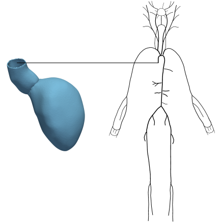
Figure 1: Left: Computational mesh of LV derived from patient-specific image-based clinical data. Right: 1D arterial network.

The biomechanical parameters of the solid and fluid models under baseline conditions have been calibrated to match a patient-specific set of in vivo measurements at specific instants of the cardiac cycle for the same subject, see [35] for further information. The same pressure-volume data is used as for the initialisation of the 3D EM model. All parameters used for the baseline case are summarised in Table 1.

5 Results

5.1 Stability assessment of the coupling method

To analyse the stability of the proposed approach, we compared the results of simulations with a varying time resolution for the 1D blood flow scheme or the 3D LV model, respectively. Taking into account the intrinsic time-step limitation necessary to ensure stability of the 1D blood flow scheme, associated with a CFL condition [36], we did not consider a time step $\mathrm{dt1D}$ higher than $110-3\text{\,}\mathrm{s}$. In more detail, in the first test case we considered $\mathrm{dt1D}\in\{$510-4\text{\,}\mathrm{s}$,$110-4\text{\,}\mathrm{s}$,$510-5\text{\,}\mathrm{s}$\}$, while keeping the time resolution for the 3D LV model constant at $\mathrm{dt3D}=$110-3\text{\,}\mathrm{s}$$. The circulatory system is represented in this case by one vessel segment of $200\text{\,}\mathrm{mm}$ and an RCR Windkessel model for terminal boundary conditions. We emphasise that the coupling is always performed at the time resolution of the 3D EM model. Figure 2 demonstrates that solutions remain unchanged when considering a different time discretisation of the circulatory model. Therefore, our results indicate that we consider the lowest temporal resolution ensuring stability of the 1D numerical scheme.

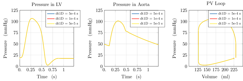
Figure 2: Illustration of model predictions. Comparison of model predictions considering different time resolutions dt1D for the 1D circulation model. Left: Pressure trace in the LV and at the inlet of the aorta. Right: Pressure-volume loop in the LV.

As a second example, we performed two simulations considering a varying time resolution for the 3D heart model, $\mathrm{dt3D}\in\{$110-3\text{\,}\mathrm{s}$,$510-4\text{\,}\mathrm{s}$\}$, keeping the same temporal resolution $\mathrm{dt1D}=$110-4\text{\,}\mathrm{s}$$ for the 1D circulatory model. Figure 3 shows that, also in this case, solutions remain unchanged when considering a different time discretisation of the 3D heart model. Thus, we will consider $\mathrm{dt3D}=$110-3\text{\,}\mathrm{s}$$ in what follows. We refer to [1] for a more detailed convergence testing of the cardiac model alone.

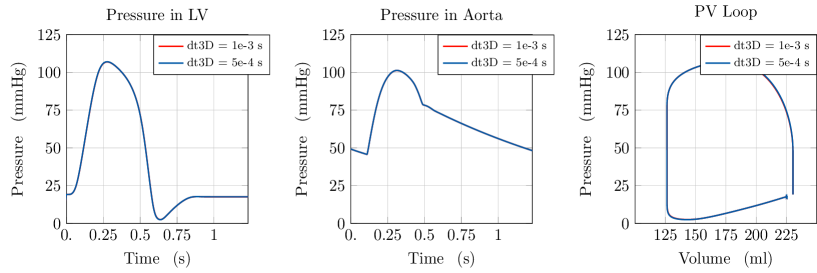
Figure 3: Illustration of model predictions. Comparison of model predictions considering different time resolutions dt3D for the 3D cardiac model. Left: Pressure trace in the LV and at the inlet of the aorta. Right: Pressure-volume loop in the LV.

5.2 Prediction of pulse wave propagation effects on cardiac function

To test the ability of the coupled model to predict the effect of pulse wave propagation on cardiac electromechanics we consider three test cases, ranging from an idealised aortic segment with a constant radius to a pathological condition called aortic coarctation and a network composed of 116 arteries.

5.2.1 Idealised aortic segment with constant radius

The first example illustrates the effect of vessel stiffening on haemodynamics and LV function. In particular, we considered a 3D LV solid model coupled to a vessel segment with constant radius and a length of $126\text{\,}\mathrm{mm}$ with lumped terminal boundary conditions. For the baseline case we set the vessel wall stiffness described by the Young modulus to $E=$0.25106\text{\,}\mathrm{Pa}$$. For two test cases with increased stiffness we set the Young modulus $E$ to $0.50106\text{\,}\mathrm{Pa}$ and $0.75106\text{\,}\mathrm{Pa}$, respectively. The 1D blood flow model was initialised using an inflow boundary condition. For the simulations in this test case we fixed $\mathrm{dt1D}=$110-4\text{\,}\mathrm{s}$$. Simulation results of the coupled model are shown in Figure 4, where the pressure trace in the LV and at the inlet of the aortic segment is compared for the different stiffness values. It can be observed that an increase in $E$ produced an increase in peak pressure and a substantial change in the shape of the pressure trace. This is due to the fact that the stiffening of the vessel wall affects pulse wave propagation in the vessel itself. In particular, the increase of aortic stiffness is associated with a premature rise and decay of the pressure wave and the well-known phenomenon of peak pressure augmentation [37]. The increased stiffness of the aortic vessel has a significant impact on LV function, see the PV loop in Figure 4 and  Figure 5. The stiffening of the arterial vessel is associated with an increase in end-systolic volume (ESV) at unchanged end-diastolic volume (EDV), leading to a reduction of stroke volume (SV)

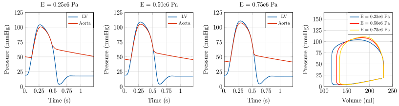
Figure 4: Illustration of model predictions. Test case 1: Idealised aortic segment with constant radius. Left: Pressure trace in the LV and at the inlet of the aorta. Right: Pressure-volume loop in the LV. Comparison of model predictions considering different Young’s modulus $E$ in the 1D blood flow model.

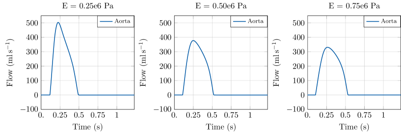
Figure 5: Illustration of model predictions. Test case 1: Idealised aortic segment with constant radius. Flow trace in the LV and at the inlet of the aorta. Comparison of model predictions considering different Young’s modulus $E$ in the 1D blood flow model.

5.2.2 Stenotic aortic segment

As a second example, we considered a pathological configuration of aortic coarctation, that is a congenital defect consisting of a local narrowing of the aortic lumen (most commonly in the aortic arch). To this end, we considered an arterial segment of $126\text{\,}\mathrm{mm}$ endowed with a stenosis model [38], with a 30% stenosis halfway of its length. Terminal boundary conditions are given by an RCR Windkessel model. In order to explore the effect of stiffening of the vessel in this configuration, we considered a baseline case with $E=$0.25106\text{\,}\mathrm{Pa}$$ and two test cases with $E$ equal to $0.50106\text{\,}\mathrm{Pa}$ and $0.75106\text{\,}\mathrm{Pa}$, respectively. For the simulations in this test case we set $\mathrm{dt1D}=$110-5\text{\,}\mathrm{s}$$ for stability considerations. Also in this example, an increase in aortic stiffness is reflected in an augmentation of peak pressure and a variation in the pressure profile, see Figure 6. The effect of vessel stiffness on LV function is shown in the PV loop of Figure 6 consists in a reduction in SV caused by an increase of the ESV.

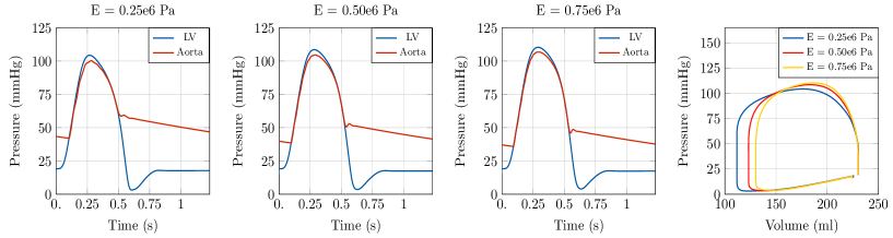
Figure 6: Illustration of model predictions. Test case 2: Aortic segment with coarctation. Left: Pressure trace in the LV and at the inlet of the aorta. Right: Pressure-volume loop in the LV. Comparison of model predictions considering different Young’s modulus $E$ in the 1D blood flow model.

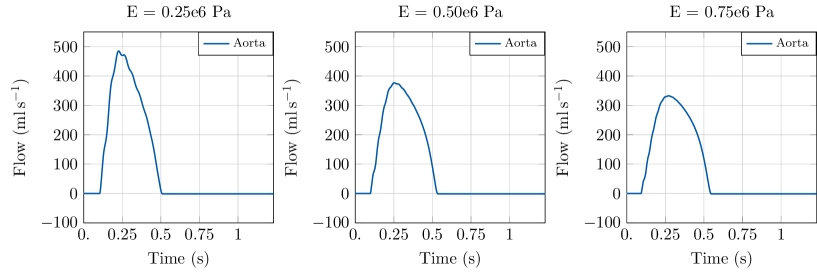
Figure 7: Illustration of model predictions. Test case 2: Aortic segment with coarctation. Flow trace in the LV and at the inlet of the aorta. Comparison of model predictions considering different Young’s modulus $E$ in the 1D blood flow model.

For the sake of completeness we show the variation of pressure and flow signals along the distance of the 1D vessel for the case $E=$0.25106\text{\,}\mathrm{Pa}$$. In particular, we show the model predictions of the 3D-1D coupled model in Figure 8.

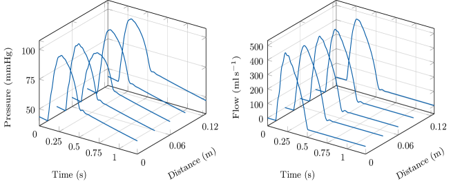
Figure 8: Illustration of model predictions. Test case 2: Aortic segment with coarctation. Pressure and flow profile in the aortic segment. Young’s modulus $E=$0.25106\text{\,}\mathrm{Pa}$$.

5.2.3 116 aortic segments

In order to explore the effect of bifurcations on pulse wave reflections and their impact on LV function the 3D EM model of the LV was coupled to a more complex model of the arterial system. To this end, as a third example we coupled the 3D model to a network consisting of 116 arterial vessels. Moreover, we explored two different physiological configurations for the 1D model, corresponding to a 25 year-old subject and a 65 year-old subject. We refer to [39] for further detail on the 1D networks considered. Concerning the 3D heart model, we considered the same parameter values as in the previous test cases, listed in Table 1, with some exceptions. In particular, the heart cycle period was set to $800\text{\,}\mathrm{ms}$ in both configurations, and the parameters of the active stress law were adapted according to the new heart cycle period. We set $\mathrm{dt1D}=$110-5\text{\,}\mathrm{s}$$ in this test case as well. Also in this example, the increase in aortic stiffness and systemic vascular resistance associated with healthy ageing is reflected in an augmentation of the peak pressure and a variation in the pressure profile, see Figure 9. The effect of ageing on LV function is also striking, as shown in  Figures 9 and 10. In particular, we can see a reduction in SV caused by an increase of the ESV. For this test case we can show the effect of pulse pressure amplification, i.e. the amplification in pulse pressure signal towards more distal locations, associated with reflections at bifurcation sites. For the sake of illustration, in Figure 11 we consider the change in pressure trace from the aortic root to the right brachial artery. As expected, pulse pressure amplification was more pronounced in the younger subject than in the 65-yo subject.

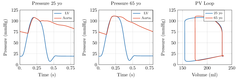
Figure 9: Illustration of model predictions. Test case 3: Network with 116 vessels. Left: Pressure trace in the LV and at the inlet of the aorta. Right: Pressure-volume loop in the LV. Comparison of model predictions considering different cardiovascular properties in the 1D blood flow model corresponding to a 25 yo and a 65 yo subject, respectively.

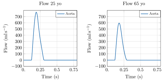
Figure 10: Illustration of model predictions. Test case 3: Network with 116 vessels. Flow trace in the LV and at the inlet of the aorta. Comparison of model predictions considering different cardiovascular properties in the 1D blood flow model corresponding to a 25 yo and a 65 yo subject, respectively.

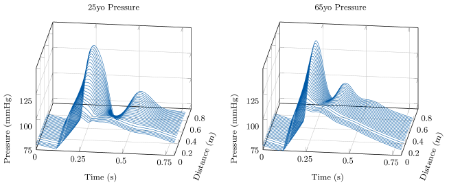
Figure 11: Illustration of model predictions. Test case 3: Network with 116 vessels. Change in pressure trace from the aortic root to the right brachial artery (in the arm). Comparison of model predictions considering different cardiovascular properties in the 1D blood flow model corresponding to a 25 yo and a 65 yo subject, respectively.

6 Discussion

In this methodological study we have developed a numerical scheme that allows to couple an advanced 3D EM model of cardiac function to a 1D model of the human circulation. First, we have demonstrated the feasibility of the proposed approach by coupling a patient-specific 3D LV model to a 1D model of the aorta and shown the ability of the model to correctly predict known physiological behaviours associated with arterial wall stiffening both in a healthy case and in the pathological case of aortic coarctation. Furthermore, we have shown an application to the coupling of the 3D LV model with a complex network composed by 116 arteries, in order to study the effect of bifurcations on pulse wave reflections and their impact on cardiovascular function.

6.1 Prediction of pulse wave propagation effects on cardiac function

The results in Section 5 show an augmentation of peak pressure in the LV and pulse pressure in the aorta and a substantial variation in the shape of the pressure trace as a consequence of stiffer vessel walls. Peak pressure in the LV increases with increasing E, since there is a higher afterload. In the aorta, the pulse pressure increases with increasing Young’s modulus E, since the aortic model becomes less compliant. Physiologically, the pulse pressure trace is composed of two additive components: first, a forward propagating wave generated by LV contraction and second, a backward propagating wave from the periphery. From this, the behaviour observed in the simulations is to be expected as the increased aortic stiffness generates a faster pulse wave propagation. Hence, this causes a premature arrival of the forward propagating wave and, in turn, of the backward propagating wave, entailing peak pressure augmentation [37].
In addition, the stiffening of the arterial vessel is related to an increase in ESV. The main reason for this effect is that a lower compliance of the vessel, i.e., its ability to distend and increase volume with increasing transmural pressure, is responsible for a reduction of blood ejected by the heart chamber, thus producing a greater ESV. Since EDV is influenced by the cardiac passive behaviour and preload rather than by afterload, this volume does not vary when the aortic vessel properties change. Hence, the stiffening of the aortic vessel leads to a reduction in SV. We have shown that the proposed 3D-1D model is capable to reproduce the impact of increased stiffness and pulsatile load in the circulation and their effect on heart performance. These results confirm that such models are particularly suited to explore the effects of changes in pulse wave propagation, which can hardly be captured using lumped parameter models [20]. Also, effects of these interactions are very complex to study in vivo due to the need for high fidelity and simultaneous measurements of cardiac function and circulation at several locations, together with the capability to assess chamber interactions [40]. Hence, 3D-1D models are of high relevance to investigate interactions between vascular waves and cardiac chamber function. Overall, a coupling to 1D models should be preferred over a coupling to lumped parameter models for clinical applications that are profoundly influenced by disrupted blood flow propagation, e.g., aortic coarctation pathologies and pulmonary arterial hypertension.

6.2 Numerical aspects

Computationally, the 3D-1D approach is comparable to 3D-0D models, as the extra cost of solving the 1D model is essentially negligible compared to the cost of the 3D model. As such, whenever wave transmission effects are to be investigated, the 3D-1D model is preferable as it can be used instead of a 3D-0D model as in [30] without any computational penalties. Further, we emphasise that the implementation of the coupling framework is not constrained to the specific choice of the 1D solver used for the solution of the blood flow equations in the circulatory system. In personalised applications the extra cost of identifying parameters of a distributed 1D system must be factored in though.

6.3 Limitations

An extension of the study is the use of more complex biventricular and four-chamber EM cardiac models [41], in order to consider the interactions among the heart chambers and thus provide more physiological simulations of the cardiac function. Also, it is well known that cardiac preload is mainly affected by venous return. As a consequence, in order to study more accurately the feedback of circulation (including venous return) on the cardiac function, the use of a 1D global model of the human circulation is more appropriate. Thus, another future perspective consists in coupling the 3D EM cardiac model with closed-loop global 1D blood flow models, e.g. [42], in order to explore the effect of circulation on preload as well. We emphasise that the coupling strategy holds for a general framework consisting of multiple cardiac cavities and is prone to different discretisations and geometries for the circulatory model, therefore such extensions are feasible. Third, this study did not specifically focus on the parameterisation of the coupled model to patient-specific data. However, the personalisation of cardiovascular models is of crucial importance for their predictive role, since the circulatory system has a complex network structure and shows a significant inter-individual variability. Owing to their distributed nature, 1D models of blood flow involve a larger amount of parameters that must be calibrated than lumped parameter models, related to geometric aspects, elastic properties and peripheral impedances of the network [10, 43]. This poses serious limitations on the applicability of the use of detailed 1D circulatory models in clinical applications. Nonetheless, there are numerous contributions in the scientific literature to cope with this problem, in terms of simplification of the geometry and reduction of the parameter set, together with the application of optimisation methods and robust inverse problem strategies. For example, the topological complexity of the arterial tree can be optimised by effectively reducing the number of arterial segments included in the 1D model, still preserving the key characteristics of flow and pressure waveforms [44, 45]. Common approaches also contemplate the rescaling of distal properties and vessel geometry based on allometric scales and global descriptors related to the geometry and properties of the network that are easy to measure, such as pulse wave velocity, body size, and biological age [46]. The level of detail of the network representing the circulatory system should be carefully considered taking into account the specific clinical application under study.
In addition, recent parameter estimation methods based on data assimilation techniques, i.e., algorithms combining mathematical models with available measurements to improve the accuracy of model predictions and estimate patient-specific parameters, have provided promising results in cardiovascular applications [47, 48, 49].

7 Conclusion

We developed a stable strategy to perform a coupling between a 3D EM model of the heart and a 1D blood flow model of the arterial system, based on the resolution of a saddle-point problem for the volume and pressure in the cavity. We built a personalised coupled 3D-1D model of LV and arterial system and showed robustness and accuracy of our scheme in a numerical benchmark. We demonstrated the ability of the coupled system to efficiently simulate physiological response to alterations in features of the circulatory system influencing pulse wave transmission, including aortic stiffening, aortic stenosis and bifurcations causing wave reflections. The additional computational costs associated with the use of 1D models instead of standard 0D models in the coupled system are negligible. As a consequence, the use of our coupled 3D-1D model is beneficial for a broad spectrum of clinical applications where wave transmission effects are under study, such as aortic coarctation and pulmonary arterial hypertension.

Appendix A Electromechanical PDE model

This section is devoted to the description of the mathematical models considered to describe the most fundamental aspects of cardiovascular function, comprising electrophysiology, passive and active mechanics and haemodynamics.

A.1 Electrophysiology

A recently developed R-E model [24] is considered for the generation of electrical activation sequences serving as a trigger for active stress generation in cardiac tissue. This hybrid R-E model combines a standard R-D model based on the monodomain equation with an eikonal model. In more detail, we consider the eikonal equation given as

$$\left\{\begin{array}[]{rcll}\sqrt{\nabla_{{\mathbf{X}}}t_{\mathrm{a}}^{\top}\,\bm{\mathbf{V}}\,\nabla_{{\mathbf{X}}}t_{\mathrm{a}}}&=&1&\text{in }\Omega_{0},\\ t_{\mathrm{a}}&=&t_{0}&\text{on }\Gamma_{0}^{\ast},\end{array}\right.$$ (6)

where $(\nabla_{{\mathbf{X}}})$ is the gradient with respect to the end-diastolic reference configuration $\Omega_{0}$, $t_{\mathrm{a}}$ is a positive function that describes the wavefront arrival time at location ${\mathbf{X}}\in\Omega_{0}$, and $t_{0}$ denote the initial activations at locations $\Gamma_{0}^{\ast}\subseteq\Gamma_{0,\mathrm{N}}$. The symmetric positive definite $3\times 3$ tensor $\bm{\mathbf{V}}({\mathbf{X}})$ contains the squared velocities $\left(v_{{\mathbf{f}}}({\mathbf{X}}),v_{{\mathbf{s}}}({\mathbf{X}}),v_{{\mathbf{n}}}({\mathbf{X}})\right)$ associated with the tissue’s eigenaxes ${\mathbf{f}}_{0}$, ${\mathbf{s}}_{0}$, and ${\mathbf{n}}_{0}$. Then, the arrival time function $t_{\mathrm{a}}({\mathbf{X}})$ is used in a modified monodomain R-D model given as

$$\beta C_{\mathrm{m}}\frac{\partial V_{\mathrm{m}}}{\partial t}=\nabla_{{\mathbf{X}}}\cdot\bm{\sigma}_{\mathrm{i}}\nabla_{{\mathbf{X}}}V_{\mathrm{m}}+I_{\mathrm{foot}}-\beta I_{\mathrm{ion}},$$ (7)

where an arrival time dependent foot current, $I_{\mathrm{foot}}(t_{\mathrm{a}})$, is added, in order to mimic sub-threshold electrotonic currents and produce a physiological foot of the action potential. The key advantage of this R-E model is that it enables to compute activation sequences at much coarser spatial resolutions without being afflicted by the spatial undersampling artefacts leading to conduction slowing or even numerical conduction blocks that are observed in standard R-D models. The tenTusscher–Noble–Noble–Panfilov model of the human ventricular myocyte [50] is employed to model Ventricular EP.

Parameter	Value	Unit	Description
Passive biomechanics
$\rho_{0}$	$1060.0$	$\mathrm{k}\mathrm{g}\mathrm{/}\mathrm{m}\mathrm{{}^{3}}$	tissue density
$\kappa$	650	$\mathrm{kPa}$	bulk modulus
$a$	0.8	$\mathrm{kPa}$	stiffness scaling
$b_{\mathrm{ff}}$	5.0	[-]	fibre strain scaling
$b_{\mathrm{ss}}$	6.0	[-]	cross-fibre in-plain strain scaling
$b_{\mathrm{nn}}$	3.0	[-]	radial strain scaling
$b_{\mathrm{fs}}$	10.0	[-]	shear strain in fibre-sheet plane scaling
$b_{\mathrm{fn}}$	2.0	[-]	shear strain in fibre-radial plane scaling
$b_{\mathrm{ns}}$	2.0	[-]	shear strain in transverse plane scaling
Active biomechanics
$\lambda_{0}$	0.7	$\mathrm{ms}$	onset of contraction
$V_{\mathrm{m,Thresh}}$	-60.0	$\mathrm{mV}$	membrane potential threshold
$t_{\mathrm{emd}}$	15.0	$\mathrm{ms}$	EM delay
$S_{\mathrm{peak}}$	60	$\mathrm{kPa}$	peak isometric tension
$t_{\mathrm{dur}}$	575.0	$\mathrm{ms}$	duration of active contraction
$\tau_{c_{0}}$	105.0	$\mathrm{ms}$	baseline time constant of contraction
$\tau_{\mathrm{r}}$	90.0	$\mathrm{ms}$	time constant of relaxation
$\mathrm{ld}$	35.0	[-]	degree of length-dependence
$\mathrm{ld}_{\mathrm{up}}$	100.0	$\mathrm{ms}$	length-dependence of upstroke time
Electrophysiology
$t_{\mathrm{cycle}}$	$1.231$	$\mathrm{s}$	cycle time ($=1/\mathrm{heartrate}$)
AA delay	20.0	$\mathrm{ms}$	inter-atrial conduction delay
AV delay	100.0	$\mathrm{ms}$	atrioventricular conduction delay
VV delay	0.0	$\mathrm{ms}$	inter-ventricular conduction delay
$(v_{\mathrm{f}},v_{\mathrm{s}},v_{\mathrm{n}})$	(0.6, 0.4, 0.2)	$\mathrm{m}\mathrm{/}\mathrm{s}$	conduction velocities
$(g_{\mathrm{f}},g_{\mathrm{s}},g_{\mathrm{n}})$	(0.44, 0.54, 0.54)	$\mathrm{m}\mathrm{/}\mathrm{s}$	conductivities in LV
$\beta$	1/1400	$\mathrm{c}\mathrm{m}^{-1}$	membrane surface-to-volume ratio
$C_{\mathrm{m}}$	1	$\mathrm{\SIUnitSymbolMicro}\mathrm{F}\mathrm{/}\mathrm{c}\mathrm{m}^{2}$	membrane capacitance

Table 1: Input parameters for the 3D PDE model of the left ventricle (lv). Adjusted to match patient-specific data.

A.2 Passive mechanics of the heart

The deformation of the heart is governed by imposed external loads such as pressure in the cavities or from surrounding tissue and active stresses intrinsically generated during contraction. The cardiac tissue is characterised as a hyperelastic, nearly incompressible, anisotropic material with a nonlinear stress-strain relationship. Mechanical deformation is described by Cauchy’s equation of motion leading to a boundary value problem

$$\rho_{0}\,\ddot{{\mathbf{u}}}(t,{\mathbf{X}})-\nabla_{{\mathbf{X}}}\cdot\mathbf{F}\mathbf{S}({\mathbf{u}},{\mathbf{X}})={\mathbf{b}}_{0}({\mathbf{X}})\quad\mbox{in }\Omega_{0},$$ (8)

for $t\in[0,T]$, where $\rho_{0}$ is the density in the Lagrange reference configuration, ${\mathbf{u}}(t,{\mathbf{X}})$ is the unknown nodal displacement, $\dot{{\mathbf{u}}}(t,{\mathbf{X}})$ is the nodal velocity, $\ddot{{\mathbf{u}}}(t,{\mathbf{X}})$ is the nodal acceleration, $\mathbf{F}({\mathbf{u}},{\mathbf{X}})$ is the deformation gradient, $\mathbf{S}({\mathbf{u}},{\mathbf{X}})$ is the second Piola–Kirchhoff stress tensor, ${\mathbf{b}}_{0}({\mathbf{X}})$ represents the body forces and $(\nabla_{{\mathbf{X}}}\;\cdot)$ denotes the divergence operator in the reference configuration. We consider as initial conditions

$${\mathbf{u}}(0,{\mathbf{X}})={\mathbf{0}},\quad\dot{{\mathbf{u}}}(0,{\mathbf{X}})={\mathbf{0}},$$

and we set ${\mathbf{b}}_{0}({\mathbf{X}})={\mathbf{0}}$ for the sake of simplicity. The boundary of the left ventricular model is decomposed in three components, i.e., $\partial\Omega_{0}=\overline{\Gamma}_{\mathrm{endo},0}\cup\overline{\Gamma}_{\mathrm{epi},0}\cup\overline{\Gamma}_{\mathrm{base},0}$, where $\overline{\Gamma}_{\mathrm{endo},0}$ denotes the endocardium, $\overline{\Gamma}_{\mathrm{epi},0}$ the epicardium, and $\overline{\Gamma}_{\mathrm{base},0}$ the base of the ventricle. At the endocardium normal stress boundary conditions are imposed:

$$\bm{\mathbf{F}}\bm{\mathbf{S}}({\mathbf{u}},{\mathbf{X}})\,{{\mathbf{n}}^{\mathrm{out}}_{0}}({\mathbf{X}})=-p(t)J\bm{\mathbf{F}}^{-\top}{{\mathbf{n}}^{\mathrm{out}}_{0}}({\mathbf{X}})\quad\text{on}\quad{\Gamma}_{\mathrm{endo},0}\times(0,T)$$ (9)

with ${{\mathbf{n}}^{\mathrm{out}}_{0}}$ the outer normal vector. Omni-directional spring type boundary conditions constrain the ventricle at the basal cut plane $\overline{\Gamma}_{\mathrm{base},0}$ [51], and spatially varying normal Robin boundary conditions are applied at the epicardium $\overline{\Gamma}_{\mathrm{epi},0}$ [52] to simulate the pericardial mechanical constrains.
We consider the following decomposition of the total stress $\mathbf{S}$:

$$\mathbf{S}=\mathbf{S}_{\mathrm{pas}}+\mathbf{S}_{\mathrm{act}},$$ (10)

where $\mathbf{S}_{\mathrm{pas}}$ and $\mathbf{S}_{\mathrm{act}}$ denote the passive and active stresses, respectively. Passive stresses are modelled according to the constitutive law

$$\mathbf{S}_{\mathrm{pas}}=2\frac{\partial\Psi(\mathbf{C})}{\partial\mathbf{C}}$$ (11)

with $\Psi$ an invariant-based strain-energy function used to model the anisotropic behaviour of cardiac tissue. Numerous constitutive models have been developed in the literature, ranging from simpler transversely-isotropic models to more complex orthotropic laws. In this article, we consider a hyper-elastic and transversely isotropic strain-energy function $\Psi$

$$\Psi_{\mathrm{Guc}}(\mathbf{C})=\frac{\kappa}{2}{\left(\log\,J\right)}^{2}+\frac{C_{\mathrm{Guc}}}{2}\left[\exp(\mathcal{Q})-1\right]$$ (12)

proposed by Guccione et al. [21]. Here, the term in the exponent is

$$\begin{split}\mathcal{Q}=\;&b_{\mathrm{f}}{({\mathbf{f}}_{0}\cdot\overline{\mathbf{E}}\,{\mathbf{f}}_{0})}^{2}+b_{\mathrm{t}}\left[{({\mathbf{s}}_{0}\cdot\overline{\mathbf{E}}\,{\mathbf{s}}_{0})}^{2}+{({\mathbf{n}}_{0}\cdot\overline{\mathbf{E}}\,{\mathbf{n}}_{0})}^{2}+2{({\mathbf{s}}_{0}\cdot\overline{\mathbf{E}}\,{\mathbf{n}}_{0})}^{2}\right]+\\ &2b_{\mathrm{fs}}\left[{({\mathbf{f}}_{0}\cdot\overline{\mathbf{E}}\,{\mathbf{s}}_{0})}^{2}+{({\mathbf{f}}_{0}\cdot\overline{\mathbf{E}}\,{\mathbf{n}}_{0})}^{2}\right]\end{split}$$ (13)

and $\overline{\mathbf{E}}=\frac{1}{2}(\overline{\mathbf{C}}-\mathbf{I})$ is the modified isochoric Green–Lagrange strain tensor, where $\overline{\mathbf{C}}:=J^{-2/3}\mathbf{C}$ with $J=\det\mathbf{F}$. Default values of $b_{\mathrm{f}}=18.48$, $b_{\mathrm{t}}=3.58$, and $b_{\mathrm{fs}}=1.627$ are used. The parameter $C_{\mathrm{Guc}}$ is used to fit the LV model to an empirical Klotz relation [53] by a combined unloading and re-inflation procedure. The bulk modulus $\kappa$, which serves as a penalty parameter to enforce nearly incompressible material behaviour, is set as $\kappa=$650\text{\,}\mathrm{kPa}$$.

Mechanics boundary conditions at the LV

The different BCs applied to the LV models are summarised in Fig. 12. The springs attached to the aortic rim and at the pericardium are shown in Fig. 12A, as well as the pressure BC in the cavity at the endocardial surface. The pericardial springs penalise displacement only in normal direction and are gradually scaled from the apex to the base. Therefore, the distance in apico-basal direction is used to create a penalty map, see Fig. 12A. To avoid non-physiological rotation, further springs are attached to the septum, see Fig. 12B. The location of the septal springs is selected automatically by constructing a local coordinate system spanned by the centres of the apical region, the MV and the AV.

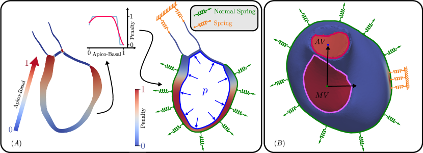
Figure 12: Boundary conditions applied to the LV models.

A.3 Active mechanics

Following the approach proposed by [22, 54], we assume that stresses due to active contraction are orthotropic, with full contractile force along the myocyte fibre orientation ${\mathbf{f}}_{0}$ and $40\text{\,}\%$ contractile force along the sheet orientation ${\mathbf{s}}_{0}$. In more detail, we define the active stress tensor $\bm{\mathbf{S}}_{\mathrm{a}}$ as

$$\bm{\mathbf{S}}_{\mathrm{a}}=S_{\mathrm{a}}{\left({\mathbf{f}}_{0}\cdot\bm{\mathbf{C}}{\mathbf{f}}_{0}\right)}^{-1}{\mathbf{f}}_{0}\otimes{\mathbf{f}}_{0}+$0.4$\,S_{\mathrm{a}}{\left({\mathbf{s}}_{0}\cdot\bm{\mathbf{C}}{\mathbf{s}}_{0}\right)}^{-1}{\mathbf{s}}_{0}\otimes{\mathbf{s}}_{0},$$ (14)

with $S_{\mathrm{a}}$ the scalar active stress that describes the contractile force. Active stress generation is modelled using a simplified phenomenological contractile model [23]. Owing to its small number of parameters and its direct relation to clinically measurable quantities such as peak pressure and the maximum rate of rise of pressure, this model is easy to fit and thus suitable for being used in clinical EM modelling studies. In particular, the active stress transient is defined as

$$S_{\mathrm{a}}(t,\lambda)=S_{\mathrm{peak}}\,\phi(\lambda)\,\tanh^{2}\left(\frac{t_{s}}{\tau_{\mathrm{c}}}\right)\,\tanh^{2}\left(\frac{t_{\mathrm{dur}}-t_{\mathrm{s}}}{\tau_{\mathrm{r}}}\right),\qquad\text{for }0<t_{\mathrm{s}}<t_{\mathrm{dur}},$$ (15)

where

$$\phi=\tanh(\mathrm{ld}(\lambda-\lambda_{0})),\quad\tau_{\mathrm{c}}=\tau_{\mathrm{c_{0}}}+\mathrm{ld}_{\mathrm{up}}(1-\phi),\quad t_{\mathrm{s}}=t-t_{\mathrm{a}}-t_{\mathrm{emd}}$$ (16)

and $t_{\mathrm{s}}$ is the onset of contraction, $\phi(\lambda)$ is a nonlinear length-dependent function in which $\lambda$ is the fibre stretch and $\lambda_{0}$ is the lower limit of fibre stretch below which no further active tension is generated, $t_{\mathrm{a}}$ is the local activation time from Eq. (6), $t_{\mathrm{emd}}$ is the EM delay between the onsets of electrical depolarisation and active stress generation, $S_{\mathrm{peak}}$ is the peak isometric tension, $t_{\mathrm{dur}}$ is the duration of active stress transient, $\tau_{\mathrm{c}}$ is time constant of contraction, $\tau_{\mathrm{c_{0}}}$ is the baseline time constant of contraction, $\mathrm{ld}_{\mathrm{up}}$ is the length-dependence of $\tau_{\mathrm{c}}$, $\tau_{\mathrm{r}}$ is the time constant of relaxation, and $\mathrm{ld}$ is the degree of length dependence. Thus, active stresses are only length-dependent in this simplified model, but dependence on fibre velocity $\dot{\lambda}$ is neglected.

Appendix B Circulatory system: 1D PDE model

In what follows, the main mathematical aspects of 1D blood flow modelling in the human circulation are detailed.

B.1 Some features of 1D blood flow modelling

The 1D equations of blood flow can be derived by integrating the Navier-Stokes equations of a generic section of the tube (after assuming axisymmetric flow in a cylindrical tube of radius $R$), obtaining

$$\begin{cases}\displaystyle\frac{\partial A}{\partial t}+\frac{\partial Q}{\partial x}=0\\[6.0pt] \displaystyle\frac{\partial Q}{\partial t}+\frac{\partial}{\partial x}\Big{(}\alpha\frac{Q^{2}}{A}\Big{)}+\frac{A}{\rho}\frac{\partial P}{\partial x}=\frac{f}{\rho},\end{cases}$$ (17)

where $A(x,t)$ is the cross-sectional area of the lumen, $Q(x,t)$ is the average flux and $P(x,t)$ is the average internal pressure over the cross-section. Note that in the momentum balance a momentum flux correction factor $\alpha$ (also known as Coriolis coefficient) is introduced, defined as

$$\alpha=\frac{1}{A\,\bar{u}^{2}}\int_{S(x,t)}u_{x}^{2}(x,t)\,\mathrm{d}\sigma$$

An energy inequality that bounds a measure of the energy of the hyperbolic system was derived in [55]. Alternatively, it is possible to rewrite the system in terms of the variables $(A,u)$. In more detail, if we assume a flat velocity profile, i.e. $\alpha=1$, we obtain the system

$$\begin{cases}\displaystyle\frac{\partial A}{\partial t}+\frac{\partial(Au)}{\partial x}=0\\[6.0pt] \displaystyle\frac{\partial u}{\partial t}+u\frac{\partial u}{\partial x}+\frac{1}{\rho}\frac{\partial P}{\partial x}=\frac{f}{\rho A},\end{cases}$$ (18)

where $A(x,t)$ is the cross-sectional area of the lumen, $u(x,t)$ is the average axial velocity and $P(x,t)$ is the average internal pressure over the cross-section.

Figure 13: Description of a 1D compliant arterial segment with properties described by a single axial coordinate x.

For a constant velocity profile satisfying the no-slip condition, the friction force per unit length is $f(x,t)=-\eta\,u(x,t)$, where $\eta$ is a coefficient depending on the blood viscosity and the average axial velocity. As System (18) is composed by two equations and three unknowns ($A,u,P$), a closure condition is needed, namely the so-called tube law:

$$P(x,t)=P_{ext}(x,t)+K\,\phi\bigl{(}A(x,t),A_{0}(x)\bigr{)}+G\,\Psi\bigl{(}A(x,t)\bigr{)},$$ (19)

where $K$ and $G$ are parameters depending on the wall stiffness and the wall viscosity, respectively.
A simple, purely elastic tube law consists in defining

$$\phi=\frac{\sqrt{A}-\sqrt{A_{0}}}{A_{0}},\ K=\frac{4}{3}\sqrt{\pi}Eh,\ \text{and}\ \Psi=0,$$

with $E$ the Young modulus and $h$ the wall thickness of the vessel. A more complex tube law is obtained when visco-elastic effects are considered, e.g., by setting

$$\Psi=\frac{1}{A_{0}\sqrt{A}}\frac{\partial A}{\partial t},\ G=\frac{2}{3}\sqrt{\pi}\varphi h,$$

with $\varphi(x)$ the wall viscosity. In what follows we consider a visco-elastic tube law, see table 2 for more detail.
In the first test cases proposed in this work we consider an arterial network consisting of a segment of the human upper thoracic aorta, equipped with a 3-element Windkessel model as a terminal boundary condition. A more complex network of vessels is also considered in Section 5.2.3, and it is taken from [39].

Parameter	Value	Unit	Description
$\rho_{0}$	$1060.0$	$\mathrm{k}\mathrm{g}\mathrm{/}\mathrm{m}\mathrm{{}^{3}}$	fluid density
$\nu$	4e-3	$\mathrm{Pa}\text{\,}\mathrm{s}$	blood flow viscosity
$\alpha$	1.1	[-]	Coriolis coefficient (momentum equation)
$G$	1	$\mathrm{kPa}$	vessel wall viscosity

Table 2: Input parameters for the 1D PDE model of the arterial circulation.

B.1.1 Boundary conditions

Standard inlet boundary conditions for 1D blood flow models consist of lumped 0D models of the heart or, alternatively, pressure or flow profiles [9, 20, 42, 43]. Every arterial 1D model must be truncated after a certain number of generations of bifurcations, since the relative size of red blood cells to vessel diameter increases, therefore the assumption made in 1D modelling that blood is a continuum and a Newtonian fluid fails. Moreover, contrary to large arteries, fluid resistance dominates over wall compliance and fluid inertia in smaller vessels. For these reasons, linear lumped parameter models are commonly employed to simulate the effect of peripheral vessels on pulse wave propagation in larger arteries [20, 56]. Such models are obtained by averaging Eq. (18) over the length of a vessel and considering some simplifying hypotheses, such as neglecting the convective term in the momentum equation. A suitable lumped parameter model for our purposes is composed of one capacitor and two resistors [57]. In more detail, the first resistance $Z$ corresponds to the characteristic aortic impedance. This is connected in series with a parallel combination of the peripheral arterial resistance $R$ and compliance $C$. We define $P_{out}$ as the pressure at which flow in the microcirculation is equal to zero. The resulting model is governed by

$$Q\Big{(}1+\frac{Z}{R}\Big{)}+C\,Z\frac{\partial{Q}}{\partial{t}}=\frac{P-P_{out}}{R}+C\frac{\partial{P_{e}}}{\partial{t}}.$$ (20)

B.1.2 Numerical implementation

Numerous models have been proposed in recent years for the numerical discretisation of the resulting system of hyperbolic equations, relying on different discretisation approaches mainly based on the finite element method (FEM) [9, 58] or finite volume method [42]. A recent benchmark study on six commonly used numerical schemes for 1D blood flow modelling [34] showed a good agreement among these schemes and their capability to capture the main characteristics of flow and pressure waveforms in the large arteries. In this study we used the solver Nektar1D [20], which is based on a FEM discretisation (discontinuous Galerkin) in space and finite difference (explicit second-order Adams–Bashforth) in time of Equations (18) and (19).

Appendix C Valve dynamics models

The EM model of the heart is coupled to the arterial network via the cardiac valves. Flow through these valves is basically triggered by a positive difference pressure between the two compartments. However, several models can be considered for modelling the dynamics of these valves, ranging from simple diode-like models to more sophisticated approaches, that are able to contemplate pathological conditions such as a stenosis or regurgitation. In the literature there are three basic approaches, ranging from simple diode-like models to more complex valve models [46], simulating a simplified valve dynamics without explicitly modelling the valve leaflets. However, when it is necessary to capture more complex flow dynamics inside the ventricles that are induced by valve pathologies, it may be required to explicitly model the shape and dynamics of the leaflets. Several approaches have been proposed [59], but this is still a very open and demanding field of research. The simplest model to simulate the action of a valve corresponds to a diode associated with a resistance (characteristic of the valve), with instant opening and closing depending on the pressure gradient upstream and downstream the valve. This model has a physiological basis, since cardiac valves open and close very rapidly (in a few milliseconds). However, it does not take into account any dynamics on $Q$, and it is not possible to model pathological conditions. As a consequence, for this work we considered a more accurate model, namely a lumped parameter model of valve dynamics proposed in [29]. Its peculiarity consists in a smooth opening and closing dynamics of the valves using a simple approach. In particular, this model is derived from the Bernoulli equation, after neglecting Poiseuille-type viscous losses (proportional to $Q$), since they are small:

$$\Delta P=B\,Q\,|Q|+L\,\dot{Q}.$$ (21)

The Bernoulli resistance $B$ is associated with the pressure difference $\Delta P$ related to convective acceleration and dynamic pressure losses caused by the diverging flow field downstream to the vena contracta, and it reads

$$B=\frac{\rho}{2\,A_{\mathrm{eff}}^{2}},$$ (22)

where $\rho$ is the blood density (usually set equal to $1060\,$\mathrm{kg}\text{\,}{\mathrm{m}}^{-3}$$) and $A_{\mathrm{eff}}$ is an effective cross-sectional area. The blood inertance $L$ is related to the pressure difference associated with blood acceleration and it is governed by the following equation:

$$L=\frac{\rho\,l_{\mathrm{eff}}}{A_{\mathrm{eff}}},$$ (23)

with $l_{\mathrm{eff}}$ an effective length, and it is here taken equal to the diameter of $A_{\mathrm{eff}}$. In order to consider valve dynamics, $A_{\mathrm{eff}}$ is a state variable and depends on an index of valve state $\xi\in[0,1]$ ($\xi=0$: closed valve, $\xi=1$: open valve) such that

$$A_{\mathrm{eff}}(t)=\big{(}A_{\mathrm{eff},\max}(t)-A_{\mathrm{eff},\min}(t)\big{)}\xi(t)+A_{\mathrm{eff},\min}(t).$$ (24)

Note that, in order to avoid division by zero in Equations (22) and (23), the valve state $\xi$ must be always strictly positive in practice. In order to consider pathological conditions like valve regurgitation, stenosis and varying annulus area $A_{\mathrm{ann}}$, the maximum $A_{\mathrm{eff},\max}$ and minimum $A_{\mathrm{eff},\min}$ effective areas can be expressed as

$$A_{\mathrm{eff},\max}(t)=M_{\mathrm{st}}A_{\mathrm{ann}}(t),\quad A_{\mathrm{eff},\min}(t)=M_{\mathrm{rg}}A_{\mathrm{ann}}(t).$$ (25)

In this study, $A_{\mathrm{ann}}$ is considered constant. The coefficients $M_{\mathrm{st}}$ and $M_{\mathrm{rg}}$ range within $[0,1]$, with $M_{\mathrm{rg}}=0$ and $M_{\mathrm{st}}=1$ in case of a healthy valve, whereas $M_{\mathrm{rg}}>0$ indicates a regurgitant valve and $M_{\mathrm{st}}<1$ stands for a stenosed valve. Finally, $M_{\mathrm{rg}}=1$ corresponds to an absent valve (unobstructed conduit), whereas $M_{\mathrm{st}}=0$ stands for an atretic valve.
The rate of valve opening and closing only depends on two factors, i.e., the instantaneous pressure difference across the valve $\Delta P$ and the current state $\xi$ of the valve. In particular, it is assumed that the valve opens when $\Delta P$ exceeds a threshold $\Delta P_{\mathrm{open}}$, and that the rate of opening is governed by

$$\frac{\mathrm{d}\xi}{\mathrm{d}t}=(1-\xi)K_{\mathrm{vo}}(\Delta P-\Delta P_{\mathrm{open}}),$$ (26)

with $K_{\mathrm{vo}}$ a rate coefficient for valve opening (in ${\mathrm{Pa}}^{-1}\text{\,}{\mathrm{s}}^{-1}$). On the other hand, it is assumed that the valve closes when $\Delta P$ is lower than a threshold $\Delta P_{\mathrm{close}}$, and that the rate of closing is governed by

$$\frac{\mathrm{d}\xi}{\mathrm{d}t}=\xi\,K_{\mathrm{vc}}(\Delta P-\Delta P_{\mathrm{close}}),$$ (27)

where $K_{vc}$ is a rate coefficient for valve closing (in ${\mathrm{Pa}}^{-1}\text{\,}{\mathrm{s}}^{-1}$). Model parameters are depicted in Table 3.

Parameter	Value	Unit	Description
Aortic Valve
$K_{\mathrm{vo}}$	2	${\mathrm{Pa}}^{-1}\text{\,}{\mathrm{s}}^{-1}$	rate coefficient for valve opening
$\Delta P_{\mathrm{open}}$	0	$\mathrm{Pa}$	threshold pressure difference for valve opening
$K_{\mathrm{vc}}$	1.2	${\mathrm{Pa}}^{-1}\text{\,}{\mathrm{s}}^{-1}$	rate coefficient for valve closing
$\Delta P_{\mathrm{close}}$	0	$\mathrm{Pa}$	threshold pressure difference for valve closing
$M_{\mathrm{st}}$	1	[-]	valve stenosis coefficient
$M_{\mathrm{rg}}$	0	[-]	valve regurgitation coefficient
Mitral Valve
$K_{\mathrm{vo}}$	0.2	${\mathrm{Pa}}^{-1}\text{\,}{\mathrm{s}}^{-1}$	rate coefficient for valve opening
$\Delta P_{\mathrm{open}}$	0	$\mathrm{Pa}$	threshold pressure difference for valve opening
$K_{\mathrm{vc}}$	0.2	${\mathrm{Pa}}^{-1}\text{\,}{\mathrm{s}}^{-1}$	rate coefficient for valve closing
$\Delta P_{\mathrm{close}}$	0	$\mathrm{Pa}$	threshold pressure difference for valve closing
$M_{\mathrm{st}}$	1	[-]	valve stenosis coefficient
$M_{\mathrm{rg}}$	0	[-]	valve regurgitation coefficient

Table 3: Input parameters for the valve dynamics model. Adjusted to match patient-specific data.

Appendix D Coupling strategy

Various approaches can be envisaged to perform the coupling between a (3D) cardiac model and a circulatory model. In practice, the problem consists in finding the new state of deformation ${\mathbf{u}}^{n+1}$ as a function of the pressure $p^{n+1}$ in the cavity applied as a Neumann boundary condition at the cavitary surface. This unknown pressure needs to be appropriately determined. Two configurations need to be captured by the model:

• When all valves are closed, the cavity is in an isovolumetric state, i.e., the muscle enclosing the cavity may deform, but the volume has to remain constant. Consequently, during an isovolumetric phase the pressure $p^{n+1}$ in the cavity needs to adjust to the variation over time of active stresses, in order to maintain the cavitary volume constant.

• When one valve is open or regurging, there is a change in cavitary volume. In this configuration the pressure $p^{n+1}$ is regulated by the state of the circulatory system or of a connected cavity. Therefore, $p^{n+1}$ needs to be estimated by matching mechanical deformation and state of the system. In fact, pressure $p^{n+1}$ in the cardiovascular system depends on flow, which depends in turn by cardiac deformation. As a consequence, the heart and circulatory models are tightly bidirectionally coupled.

From a mathematical perspective, this coupling can be performed in two ways. The simplest approach is to prescribe $p^{n+1}$ explicitly. Then, the coupling is performed during the ejection phase by updating flow and flow rate based on the current prediction on the change in the state of deformation associated with the currently predicted pressure $p^{n+1}$. In particular, the pressure boundary condition in each nonlinear solver step is modified within each iteration ${\nu}$. Note that the new prediction $p^{n+1}_{\nu+1}$ is then explicitly prescribed as a Neumann boundary condition. Therefore, this explicit and partitioned approach may introduce some inaccuracies during ejection phases and can lead to instabilities during isovolumetric phases. Such instabilities arise from the difficulty of estimating the change in pressure necessary to keep the volume constant. In fact, a knowledge on cavitary elastance is required to know the $p-V$ relation of the cavity at this given point in time, that is not available. Therefore, iterative estimates are needed to gradually inflate or deflate a cavity to its prescribed volume. However, since the elastance properties of the cavities are highly nonlinear, an overestimation may induce oscillations, whereas an underestimation may induce very slow convergence and prohibitively large numbers of Newton iterations. A more sophisticated approach consists in treating $p^{n+1}$ as an unknown. Thus, an additional equation is required to close the system, leading to a saddle point formulation and a block system to be solved (monolithic approach).

Isovolumetric Phases

During the isovolumetric phases we can state that

$$\operatorname{V}^{\mathrm{heart}}_{c}({\mathbf{u}})-V_{0}=0,$$

i.e., the volume of each cavity ${V}^{\mathrm{heart}}_{c}({\mathbf{u}})$ equals an initial volume $V_{0}$ and does not change during the isovolumetric phase. Hence, in system (4) the matrix $\bm{\mathbf{C}}^{\prime}(\underline{p}_{k})=\bm{\mathbf{0}}$ and $V^{\mathrm{CS}}(\underline{p}_{k})=V_{0}$.

Appendix E Finite Element Formulation

E.1 Variational Formulation

For the sake of simplicity of formulation, we neglect here the acceleration term in Eq. (3) in this section and consider at the stationary counterpart of the boundary value problem (8–9) with (1). Please refer to [30] for further detail on the full nonlinear elastodynamics problem. The boundary value problem (8–9) with (1) can be formally expressed in terms of the equations

$$\langle\mathcal{A}_{0}({\mathbf{u}}),{\mathbf{v}}\rangle_{\Omega_{0}}-\langle\mathcal{F}_{0}({\mathbf{u}},p_{c}),{\mathbf{v}}\rangle_{\Omega_{0}} ={\mathbf{0}},$$ (28)

$$\langle V_{c}^{\mathrm{heart}}({\mathbf{u}}),q\rangle_{\Omega_{0}}-\langle V_{c}^{\mathrm{CS}}(p_{c}),q\rangle_{\Omega_{0}} =0,$$ (29)

which is valid for all vector fields ${\mathbf{v}}$ smooth enough and vanishing on the Dirichlet boundary ${\Gamma}_{0,\mathrm{D}}$, test functions $q$ that are $1$ for the cavity $c\in\{\mathrm{LV,RV,LA,RA}\}$ and $0$ otherwise, with the duality pairing $\langle\cdot,\cdot\rangle_{\Omega_{0}}$. The first term on the left hand side of the variational Eq. (28) represents the rate of internal mechanical work and is defined as

$$\langle\mathcal{A}_{0}({\mathbf{u}}),{\mathbf{v}}\rangle_{\Omega_{0}}:=\int_{\Omega_{0}}\bm{\mathbf{S}}({\mathbf{u}}):\bm{\mathbf{\Sigma}}({\mathbf{u}},{\mathbf{v}})\,\mathrm{d}{\mathbf{X}},$$ (30)

where $\bm{\mathbf{S}}$ denotes the second Piola–Kirchhoff stress tensor, see (10), and $\bm{\mathbf{\Sigma}}({\mathbf{u}},{\mathbf{v}})$ is the directional derivative of the Green–Lagrange strain tensor, see [1, 60]. The second term on the left hand side denotes the weak form of the contribution of pressure loads (28) and is computed using (9)

$$\langle\mathcal{F}_{0}({\mathbf{u}},p_{c}),{\mathbf{v}}\rangle_{\Omega_{0}}=-p_{c}\int\limits_{\Gamma_{0,\mathrm{N}}}J\,\bm{\mathbf{F}}^{-\top}({\mathbf{u}})\,{{\mathbf{n}}^{\mathrm{out}}_{0}}\cdot{\mathbf{v}}\,\,\mathrm{d}s_{{\mathbf{X}}}.$$ (31)

The first term of the coupling equation (29) is obtained from (2) using Nanson’s formula and ${\mathbf{x}}={\mathbf{X}}+{\mathbf{u}}$ by

$$\langle V_{c}^{\mathrm{heart}}({\mathbf{u}}),q\rangle_{\Omega_{0}}=\frac{1}{3}\int\limits_{\Gamma_{0,\mathrm{N}}}({\mathbf{X}}+{\mathbf{u}})\cdot J\bm{\mathbf{F}}^{-\top}{{\mathbf{n}}^{\mathrm{out}}_{0}}\,q\,\mathrm{d}s_{{\mathbf{X}}}.$$ (32)

The second term of (29) is computed using the 1D blood flow model, see B, for $c\in\{\mathrm{LV,RV,LA,RA}\}$.

E.2 Consistent Linearisation

A Newton–Raphson scheme is employed to solve the nonlinear variational equations (28)–(29), with a finite element approach see [61]. Let us consider a nonlinear and continuously differentiable operator $F\colon X\to Y$. Then, a solution to $F(x)=0$ can be approximated by

$$x^{k+1} =x^{k}+\Delta x,$$

$$\left.\frac{\partial F}{\partial x}\right|_{x=x^{k}}\Delta x =-F(x^{k}),$$

which is evaluated until convergence. In our approach, we assume $X=\left[H^{1}(\Omega_{0},\Gamma_{0,\mathrm{D}})\right]^{3}\times\mathbb{R}$, $Y=\mathbbm{R}^{2}$, $\Delta x={(\Delta{\mathbf{u}},\Delta p_{c})}^{\top}$, $x^{k}={({\mathbf{u}}^{k},p_{c}^{k})}^{\top}$, and $F={(R_{{\mathbf{u}}},R_{\mathrm{p}})}^{\top}$. Thus, we obtain the following linearised saddle-point problem for each $({\mathbf{u}}^{k},p_{c}^{k})\in\left[H^{1}(\Omega_{0},\Gamma_{0,\mathrm{D}})\right]^{3}\times\mathbb{R}$, find $(\Delta{\mathbf{u}},\Delta p_{c})\in\left[H^{1}_{0}(\Omega_{0})\right]^{3}\times\mathbb{R}$ such that

$$\langle\Delta{\mathbf{u}},A_{0}^{\prime}({\mathbf{u}}^{k})\,{\mathbf{v}}\rangle_{\Omega_{0}}+\langle\Delta{\mathbf{u}},\mathcal{F}_{0}^{\prime}({\mathbf{u}}^{k},p_{c}^{k})\,{\mathbf{v}}\rangle_{\Omega_{0}}$$

$$+\langle\Delta p_{c},\mathcal{F}_{0}^{\prime}({\mathbf{u}}^{k},p_{c}^{k})\,{\mathbf{v}}\rangle_{\Omega_{0}} =-\langle R_{{\mathbf{u}}}({\mathbf{u}}^{k},p_{c}^{k}),{\mathbf{v}}\rangle_{\Omega_{0}},$$ (33)

$$\langle\Delta{\mathbf{u}},V_{c}^{\mathrm{heart}}({\mathbf{u}}^{k})\,q\rangle_{\Omega_{0}}-\langle\Delta p_{c},V_{c}^{\mathrm{CS}}(p_{c}^{k})\,q\rangle_{\Omega_{0}} =-\langle R_{\mathrm{p}}({\mathbf{u}}^{k},p_{c}^{k}),q\rangle_{\Omega_{0}},$$ (34)

with the updates

$${\mathbf{u}}^{k+1} ={\mathbf{u}}^{k}+\Delta{\mathbf{u}},$$ (35)

$$p_{c}^{k+1} =p_{c}^{k}+\Delta p_{c}.$$ (36)

The Gâteaux derivative of (28) with respect to the displacement change update $\Delta{\mathbf{u}}$ yields the first term in (E.2)

$$\langle\Delta{\mathbf{u}},A_{0}^{\prime}({\mathbf{u}}^{k})\,{\mathbf{v}}\rangle_{\Omega_{0}}: =\left.D_{\Delta{\mathbf{u}}}\langle\mathcal{A}_{0}({\mathbf{u}}),{\mathbf{v}}\rangle_{\Omega_{0}}\right|_{{\mathbf{u}}={\mathbf{u}}^{k}}$$

$$=\int\limits_{\Omega_{0}}\bm{\mathbf{S}}_{k}:\bm{\mathbf{\Sigma}}(\Delta{\mathbf{u}},{\mathbf{v}})\,\mathrm{d}{\mathbf{X}}+\int\limits_{\Omega_{0}}\bm{\mathbf{\Sigma}}({\mathbf{u}}^{k},\Delta{\mathbf{u}}):\mathbbm{C}_{k}:\bm{\mathbf{\Sigma}}({\mathbf{u}}^{k},{\mathbf{v}})\,\mathrm{d}{\mathbf{X}},$$ (37)

and the second term in (E.2), that is given by

$$\langle\Delta{\mathbf{u}},\mathcal{F}_{0}^{\prime}({\mathbf{u}}^{k},p_{c}^{k})\,{\mathbf{v}}\rangle_{\Omega_{0}}: =\left.D_{\Delta{\mathbf{u}}}\langle\mathcal{F}_{0}({\mathbf{u}},p_{c}),{\mathbf{v}}\rangle_{\Omega_{0}}\right|_{{\mathbf{u}}={\mathbf{u}}^{k},p_{c}=p_{c}^{k}}$$

$$=p^{k}_{c}\int_{\Gamma_{0,\mathrm{N}}}J_{k}\bm{\mathbf{F}}_{k}^{-\top}\operatorname{Grad}^{\top}\!\Delta{\mathbf{u}}\,\bm{\mathbf{F}}_{k}^{-\top}{{\mathbf{n}}^{\mathrm{out}}_{0}}\cdot{\mathbf{v}}\,\,\mathrm{d}s_{{\mathbf{X}}}$$

$$-p^{k}_{c}\int_{\Gamma_{0,\mathrm{N}}}J_{k}(\bm{\mathbf{F}}_{k}^{-\top}:\operatorname{Grad}\Delta{\mathbf{u}})\,\bm{\mathbf{F}}_{k}^{-\top}{{\mathbf{n}}^{\mathrm{out}}_{0}}\cdot{\mathbf{v}}\,\,\mathrm{d}s_{{\mathbf{X}}},$$ (38)

where we have defined, for the sake of simplicity:

$$\bm{\mathbf{F}}_{k} :=\bm{\mathbf{F}}({\mathbf{u}}^{k}),\ J_{k}:=\det(\bm{\mathbf{F}}^{k}),\ \bm{\mathbf{S}}_{k}:=\left.\bm{\mathbf{S}}\right|_{{\mathbf{u}}={\mathbf{u}}^{k}},\ \mathbbm{C}_{k}:=\left.\mathbbm{C}\right|_{{\mathbf{u}}={\mathbf{u}}^{k}}.$$

The third term in (E.2) is defined using the Gâteaux derivative of (28) with respect to the pressure change update $\Delta p_{c}$:

$$\langle\Delta p_{c},\mathcal{F}_{0}^{\prime}({\mathbf{u}}^{k},p_{c}^{k})\,{\mathbf{v}}\rangle_{\Omega_{0}}: =\left.D_{\Delta p_{c}}\langle\mathcal{F}_{0}({\mathbf{u}},p_{c}),{\mathbf{v}}\rangle_{\Omega_{0}}\right|_{{\mathbf{u}}={\mathbf{u}}^{k},p_{c}=p_{c}^{k}}$$

$$=-\Delta p_{c}\int_{\Gamma_{0,\mathrm{N}}}J_{k}\,\bm{\mathbf{F}}_{k}^{-\top}\,{{\mathbf{n}}^{\mathrm{out}}_{0}}\cdot{\mathbf{v}}\,\,\mathrm{d}s_{{\mathbf{X}}}.$$ (39)

The right hand side of (E.2) depends on the residual $R_{{\mathbf{u}}}$, and it is defined as

$$\langle R_{{\mathbf{u}}}({\mathbf{u}}^{k},p_{c}^{k}),{\mathbf{v}}\rangle_{\Omega_{0}}:=\langle A_{0}({\mathbf{u}}^{k}),{\mathbf{v}}\rangle_{\Omega_{0}}-\langle{\mathbf{\mathcal{F}}}_{0}({\mathbf{u}}^{k},p_{c}^{k}),{\mathbf{v}}\rangle_{\Omega_{0}}.$$ (40)

From (32), using the known relations [60],

$$\frac{\partial J}{\partial\bm{\mathbf{F}}}:\operatorname{Grad}\Delta{\mathbf{u}} =J\bm{\mathbf{F}}^{-\top}:\operatorname{Grad}\Delta{\mathbf{u}}$$

$$\frac{\partial\bm{\mathbf{F}}^{-\top}}{\partial\bm{\mathbf{F}}}:\operatorname{Grad}\Delta{\mathbf{u}} =-\bm{\mathbf{F}}^{-\top}{(\operatorname{Grad}\Delta{\mathbf{u}})}^{\top}\bm{\mathbf{F}}^{-\top}$$

we can define the first term of (34) as the Gâteaux derivative with respect to the update $\Delta{\mathbf{u}}$

$$\langle\Delta{\mathbf{u}},V_{c}^{\mathrm{heart}}({\mathbf{u}}^{k})\,q\rangle_{\Omega_{0}}: =\left.D_{\Delta{\mathbf{u}}}\langle V_{c}^{\mathrm{heart}}({\mathbf{u}}),q\rangle_{\Omega_{0}}\right|_{{\mathbf{u}}={\mathbf{u}}^{k}}$$

$$=D_{\Delta{\mathbf{u}}}\frac{1}{3}\int_{\Gamma_{0,\mathrm{N}}}\left({\mathbf{X}}+{\mathbf{u}}^{k}\right)\cdot J_{k}\bm{\mathbf{F}}_{k}^{-\top}{{\mathbf{n}}^{\mathrm{out}}_{0}}\,q\,\mathrm{d}s_{{\mathbf{X}}}$$

$$=\frac{1}{3}\int_{\Gamma_{0,\mathrm{N}}}J_{k}(\bm{\mathbf{F}}_{k}^{-\top}:\operatorname{Grad}\Delta{\mathbf{u}}){\mathbf{x}}\cdot\bm{\mathbf{F}}_{k}^{-\top}{{\mathbf{n}}^{\mathrm{out}}_{0}}\,q\,\mathrm{d}s_{{\mathbf{X}}}$$

$$\quad-\frac{1}{3}\int_{\Gamma_{0,\mathrm{N}}}J_{k}{\mathbf{x}}\cdot\bm{\mathbf{F}}_{k}^{-\top}{(\operatorname{Grad}\Delta{\mathbf{u}})}^{\top}\bm{\mathbf{F}}_{k}^{-\top}{{\mathbf{n}}^{\mathrm{out}}_{0}}\,q\,\mathrm{d}s_{{\mathbf{X}}}$$

$$\quad+\frac{1}{3}\int_{\Gamma_{0,\mathrm{N}}}J_{k}\Delta{\mathbf{u}}\cdot\bm{\mathbf{F}}_{k}^{-\top}{{\mathbf{n}}^{\mathrm{out}}_{0}}\,q\,\mathrm{d}s_{{\mathbf{X}}},$$ (41)

where $q$ is a test function with value $1$ for the surface $\Gamma_{0,c}$ of cavity $c$, and $0$ otherwise.

The second term of (34) is defined as the numerical derivative

$$\langle\Delta p_{c},V_{c}^{\mathrm{CS}}(p_{c}^{k})\,q\rangle_{\Omega_{0}}: =\left.D_{\Delta p_{c}}\langle V_{c}^{\mathrm{CS}}(p_{c})\,q\rangle_{\Omega_{0}}\right|_{p_{c}=p_{c}^{k}}$$

$$=\frac{1}{\epsilon}\left(V_{c}^{\mathrm{CS}}(p_{c}^{k}+\epsilon)-V_{c}^{\mathrm{CS}}(p_{c}^{k})\right)q,$$ (42)

with $\epsilon=p_{c}^{k}\sqrt{\epsilon_{\mathrm{m}}}$ chosen according to [62, Chapter 5.7], and $\epsilon_{\mathrm{m}}=2^{-52}\approx 2.2*10^{-16}$ is the machine accuracy.

Finally, the right hand side of (34), is defined based on the residual $R_{\mathrm{p}}$ and reads

$$\langle R_{\mathrm{p}}({\mathbf{u}}^{k},p_{c}^{k}),q\rangle_{\Omega_{0}}:=\langle V_{c}^{\mathrm{heart}}({\mathbf{u}}),q\rangle_{\Omega_{0}}-\langle V_{c}^{\mathrm{CS}}(p_{c}),q\rangle_{\Omega_{0}}.$$ (43)

Assembling of the block matrices

The finite element method (FEM) relies on the definition of an admissible decomposition of the computational domain $\Omega\subset\mathbbm{R}^{3}$ into $M$ tetrahedral elements $\tau_{j}$ and the introduction of a conformal finite element space

$$X_{h}\subset H^{1}(\Omega_{0}),\ N=\text{dim}\,X_{h}$$

of piecewise polynomial continuous basis functions $\varphi_{i}$. After linearising the variational problem (E.2)–(34) and considering a Galerkin finite element discretisation, we obtain a block system to be solved. The problem then reads: find $\delta\underline{u}\in\mathbbm{R}^{3N}$ and $\delta\underline{p}_{c}\in\mathbbm{R}^{N_{\mathrm{cav}}}$ such that

$$\begin{pmatrix}(\bm{\mathbf{A}}^{\prime}-\bm{\mathbf{M}}^{\prime})(\underline{u}^{k},\underline{p}_{c}^{k})&\bm{\mathbf{B}}^{\prime}_{\mathrm{p}}(\underline{u}^{k})\\ \bm{\mathbf{B}}^{\prime}_{{\mathbf{u}}}(\underline{u}^{k})&\bm{\mathbf{C}}^{\prime}(\underline{p}_{c}^{k})\\ \end{pmatrix}\begin{pmatrix}\delta\underline{u}\\ \delta\underline{p}_{c}\end{pmatrix} =-\begin{pmatrix}\underline{A}(\underline{u}^{k})-\underline{B}_{\mathrm{p}}(\underline{u}^{k},\underline{p}_{c}^{k})\\ \underline{V}_{c}^{\mathrm{heart}}(\underline{u}^{k})-\underline{V}_{c}^{\mathrm{CS}}(\underline{p}_{c}^{k})\end{pmatrix},$$ (44)

$$\underline{u}^{k+1} =\underline{u}^{k}+\delta\underline{u},$$ (45)

$$\underline{p}_{c}^{k+1} =\underline{p}_{c}^{k}+\delta\underline{p}_{c}$$ (46)

with the solution vectors $\underline{u}^{k}\in\mathbbm{R}^{3N}$ and $\underline{p}_{c}^{k}\in\mathbbm{R}^{N_{\mathrm{cav}}}$ at the $k$-th Newton step. The tangent stiffness matrix $\bm{\mathbf{A}}^{\prime}\in\mathbbm{R}^{3N\times 3N}$ is computed from (37) as follows:

$$\bm{\mathbf{A}}^{\prime}(\underline{u}^{k})[j,i]:=\langle\bm{\varphi}_{i},\mathcal{A}_{0}^{\prime}({\mathbf{u}}^{k})\,\bm{\varphi}_{j}\rangle_{\Omega_{0}}.$$ (47)

The mass matrix $\bm{\mathbf{M}}^{\prime}\in\mathbbm{R}^{3N\times 3N}$ is calculated from (38) and reads

$$\bm{\mathbf{M}}^{\prime}(\underline{u}^{k},\underline{p}_{c}^{k})[j,i]:=\langle\bm{\varphi}_{i},\mathcal{F}_{0}^{\prime}({\mathbf{u}}^{k},p_{c}^{k})\,\bm{\varphi}_{j}\rangle_{\Omega_{0}}.$$ (48)

The off-diagonal matrices $\bm{\mathbf{B}}^{\prime}_{{\mathbf{u}}}\in\mathbbm{R}^{3N\times N_{\mathrm{cav}}}$ and $\bm{\mathbf{B}}^{\prime}_{\mathrm{p}}\in\mathbbm{R}^{N_{\mathrm{cav}}\times 3N}$ in (44) are assembled using (41)

$$\bm{\mathbf{B}}^{\prime}_{{\mathbf{u}}}(\underline{u}^{k},\underline{p}_{c}^{k})[i,j]=\langle\underline{\varphi}_{j},V_{c}^{\mathrm{heart}}({\mathbf{u}}^{k})\hat{\varphi_{i}}\rangle_{\Omega_{0}},\quad i=1,\dots,N_{\mathrm{cav}}$$ (49)

and (39)

$$\bm{\mathbf{B}}^{\prime}_{\mathrm{p}}(\underline{u}^{k},\underline{p}_{c}^{k})[i,j]=\langle\hat{\varphi_{j}},\mathcal{F}_{0}^{\prime}({\mathbf{u}}^{k},p_{c}^{k})\bm{\varphi}_{i}\rangle_{\Omega_{0}},\quad j=1,\dots,N_{\mathrm{cav}},$$ (50)

where the constant shape functions have value $\hat{\varphi_{j}}=1$ if $\tau_{j}\in\Gamma_{0,c}$ and $\hat{\varphi_{j}}=0$ if $\tau_{j}\notin\Gamma_{0,c}$ for $c\in\{\mathrm{LV,RV,LA,RA}\}$.

Considering the approach described in [63, Sect. 4.2], this assembling procedure can be simplified for closed cavities such that

$$\bm{\mathbf{B}}^{\prime}_{\mathrm{p}}(\underline{u}^{k},\underline{p}_{c}^{k})={\left[\bm{\mathbf{B}}^{\prime}_{{\mathbf{u}}}(\underline{u}^{k},\underline{p}_{c}^{k})\right]}^{\top}.$$

Then, the circulatory compliance matrix $\bm{\mathbf{C}}^{\prime}(\underline{p}_{c}^{k})\in\mathbbm{R}^{N_{\mathrm{cav}}\times N_{\mathrm{cav}}}$ is computed from (42) as

$$\bm{\mathbf{C}}^{\prime}(\underline{p}_{c}^{k})[i,j]=\langle\hat{\varphi_{j}},V_{c}^{\mathrm{CS}}(p_{c}^{k})\,\hat{\varphi_{i}}\rangle_{\Omega_{0}},\quad i,j=1,\dots,N_{\mathrm{cav}},$$ (51)

with the constant shape function $\hat{\varphi_{j}}=1$ if $\tau_{j}\in\Gamma_{0,c}$ and $\hat{\varphi_{j}}=0$ if $\tau_{j}\notin\Gamma_{0,c}$ for $c\in\{\mathrm{lv,rv,la,ra}\}$, leading to a diagonal matrix. The terms on the right hand side $\underline{A}\in\mathbbm{R}^{3N}$, $\underline{B}_{\mathrm{p}}\in\mathbbm{R}^{3N}$ are constructed using (40) and read

$$\underline{A}(\underline{u}^{k})[i]:=\langle\mathcal{A}_{0}({\mathbf{u}}^{k}),\bm{\varphi}_{i}\rangle_{\Omega_{0}}$$ (52)

and

$$\underline{B}_{\mathrm{p}}(\underline{u}^{k},\underline{p}_{c}^{k})[i]:=\langle\mathcal{F}_{0}({\mathbf{u}}^{k},p_{c}^{k}),\bm{\varphi}_{i}\rangle_{\Omega_{0}},$$ (53)

see also [1, 60]. Finally, the terms $\underline{V}_{c}^{\mathrm{heart}}\in\mathbbm{R}^{N_{\mathrm{cav}}}$ and $\underline{V}_{c}^{\mathrm{CS}}\in\mathbbm{R}^{N_{\mathrm{cav}}}$ in lower right hand side in (44) are assembled from (43) and are given by:

$$\underline{V}_{c}^{\mathrm{heart}}(\underline{u}^{k})[i]=\langle V_{c}^{\mathrm{heart}}({\mathbf{u}}),\hat{\varphi_{i}}\rangle_{\Omega_{0}},\quad i=1,\dots,N_{\mathrm{cav}},$$ (54)

and

$$\underline{V}_{c}^{\mathrm{CS}}(\underline{p}_{c}^{k})[i]=\langle V_{c}^{\mathrm{CS}}(p_{c}),\hat{\varphi_{i}}\rangle_{\Omega_{0}},\quad i=1,\dots,N_{\mathrm{cav}}.$$ (55)

Appendix F Direct Schur Complement Solver for a Small Number of Constraints

Let us consider the block system $\bm{\mathbf{K}}\in\mathbbm{R}^{n\times n}$, $\bm{\mathbf{C}}\in\mathbbm{R}^{m\times m}$

$$\begin{pmatrix}\bm{\mathbf{K}}&\bm{\mathbf{A}}\\ \bm{\mathbf{B}}&\bm{\mathbf{C}}\end{pmatrix}\begin{pmatrix}\underline{u}\\ \underline{p}\end{pmatrix}=-\begin{pmatrix}\underline{f}\\ \underline{g}\end{pmatrix}$$

with

$$\bm{\mathbf{A}}=\begin{pmatrix}\underline{a}_{1}&\!\!\!\vrule\!\!\!&\cdots&\!\!\!\vrule\!\!\!&\underline{a}_{m}\end{pmatrix}\in\mathbbm{R}^{n\times m},\quad\bm{\mathbf{B}}=\begin{pmatrix}\underline{b}_{1}&\!\!\!\vrule\!\!\!&\cdots&\!\!\!\vrule\!\!\!&\underline{b}_{m}\end{pmatrix}^{\top}\in\mathbbm{R}^{m\times n}.$$

We can write the Schur complement system as

$$(\bm{\mathbf{B}}\bm{\mathbf{K}}^{-1}\bm{\mathbf{A}}-\bm{\mathbf{C}})\underline{p} =\underline{g}-\bm{\mathbf{B}}\bm{\mathbf{K}}^{-1}\underline{f}$$

$$\underline{u} =\bm{\mathbf{K}}^{-1}\underline{f}-\bm{\mathbf{K}}^{-1}\bm{\mathbf{A}}\underline{p}.$$

With

$$\underline{r}=\bm{\mathbf{K}}^{-1}\underline{f},\quad\bm{\mathbf{S}}=\bm{\mathbf{K}}^{-1}\underline{A}=\begin{pmatrix}\underline{s}_{1}&\!\!\!\vrule\!\!\!&\cdots&\!\!\!\vrule\!\!\!&\underline{s}_{m}\end{pmatrix}\in\mathbbm{R}^{n\times m},\ \underline{s}_{i}=\bm{\mathbf{K}}^{-1}\underline{a}_{i},\ i=1,\dots,m$$ (56)

we obtain

$$(\bm{\mathbf{B}}\bm{\mathbf{S}}-\bm{\mathbf{C}})\underline{p} =\underline{g}-\bm{\mathbf{B}}\underline{r}$$

$$\underline{u} =\underline{r}-\bm{\mathbf{S}}\underline{p}.$$ (57)

The realisation of (57) involves $m+1$ solves and the inversion of an $m\times m$ matrix. As $m$ is generally small, this can be done symbolically.

$${[\bm{\mathbf{B}}\bm{\mathbf{S}}]}_{ij}=\underline{b}_{i}\cdot\underline{s}_{j},\ \mbox{for}\ i,j=1,\dots,m.$$

References

- Augustin et al. [2016] C. M. Augustin, A. Neic, M. Liebmann, A. J. Prassl, S. A. Niederer, G. Haase, G. Plank, Anatomically accurate high resolution modeling of human whole heart electromechanics: a strongly scalable algebraic multigrid solver method for nonlinear deformation, Journal of Computational Physics 305 (2016) 622–646.
- Niederer et al. [2019] S. A. Niederer, J. Lumens, N. A. Trayanova, Computational models in cardiology, Nature Reviews Cardiology 16 (2) (2019) 100–111.
- Diaz-Zuccarini et al. [2013] V. Diaz-Zuccarini, M. Viceconti, V. Stroetmann, D. Kalra, Roadmap for the digital patient, The Digital Patient Community and the Discipulus Consortium: EU Project Discipulus .
- Chabiniok et al. [2016] R. Chabiniok, V. Y. Wang, M. Hadjicharalambous, L. Asner, J. Lee, M. Sermesant, E. Kuhl, A. A. Young, P. Moireau, M. P. Nash, et al., Multiphysics and multiscale modelling, data–model fusion and integration of organ physiology in the clinic: ventricular cardiac mechanics, Interface focus 6 (2) (2016) 20150083.
- Corral-Acero et al. [2020] J. Corral-Acero, F. Margara, M. Marciniak, C. Rodero, F. Loncaric, Y. Feng, A. Gilbert, J. F. Fernandes, H. A. Bukhari, A. Wajdan, et al., The Digital Twin to enable the vision of precision cardiology, European heart journal 41 (48) (2020) 4556–4564.
- Westerhof et al. [2009] N. Westerhof, J.-W. Lankhaar, B. E. Westerhof, The arterial windkessel, Medical & biological engineering & computing 47 (2) (2009) 131–141.
- Segers et al. [2003] P. Segers, N. Stergiopulos, N. Westerhof, P. Wouters, P. Kolh, P. Verdonck, Systemic and pulmonary hemodynamics assessed with a lumped-parameter heart-arterial interaction model, J Eng Math 47 (3-4) (2003) 185–199.
- Segers et al. [2008] P. Segers, E. Rietzschel, M. De Buyzere, N. Stergiopulos, N. Westerhof, L. Van Bortel, T. Gillebert, P. Verdonck, Three-and four-element Windkessel models: assessment of their fitting performance in a large cohort of healthy middle-aged individuals, Proc Inst Mech Eng H 222 (4) (2008) 417–428.
- Formaggia et al. [2003] L. Formaggia, D. Lamponi, A. Quarteroni, One-dimensional models for blood flow in arteries, Journal of Engineering Mathematics 47 (2003) 251–276.
- Reymond et al. [2011] P. Reymond, Y. Bohraus, F. Perren, F. Lazeyras, N. Stergiopulos, Validation of a patient-specific one-dimensional model of the systemic arterial tree, American Journal of Physiology - Heart and Circulatory Physiology 301 (3) (2011) H1173–H1182, ISSN 0363-6135.
- Manganotti et al. [2021] J. Manganotti, F. Caforio, F. Kimmig, P. Moireau, S. Imperiale, Coupling reduced-order blood flow and cardiac models through energy-consistent strategies: modeling and discretization, Advanced Modeling and Simulation in Engineering Sciences 8 (1) (2021) 21.
- Van de Vosse and Stergiopulos [2011] F. N. Van de Vosse, N. Stergiopulos, Pulse wave propagation in the arterial tree, Annual Review of Fluid Mechanics 43 (2011) 467–499.
- Sainte-Marie et al. [2006] J. Sainte-Marie, D. Chapelle, R. Cimrman, M. Sorine, Modeling and estimation of the cardiac electromechanical activity, Computers & structures 84 (28) (2006) 1743–1759.
- Kerckhoffs et al. [2007] R. C. Kerckhoffs, M. L. Neal, Q. Gu, J. B. Bassingthwaighte, J. H. Omens, A. D. McCulloch, Coupling of a 3D finite element model of cardiac ventricular mechanics to lumped systems models of the systemic and pulmonic circulation, Annals of biomedical engineering 35 (1) (2007) 1–18.
- Nordsletten et al. [2011] D. Nordsletten, S. Niederer, M. Nash, P. Hunter, N. Smith, Coupling multi-physics models to cardiac mechanics, Progress in biophysics and molecular biology 104 (1-3) (2011) 77–88.
- Hirschvogel et al. [2017] M. Hirschvogel, M. Bassilious, L. Jagschies, S. M. Wildhirt, M. W. Gee, A monolithic 3D-0D coupled closed-loop model of the heart and the vascular system: Experiment-based parameter estimation for patient-specific cardiac mechanics, International journal for numerical methods in biomedical engineering 33 (8) (2017) e2842.
- Regazzoni et al. [2020] F. Regazzoni, M. Salvador, P. C. Africa, M. Fedele, L. Dede, A. Quarteroni, A cardiac electromechanics model coupled with a lumped parameters model for closed-loop blood circulation. Part I: model derivation, arXiv preprint arXiv:2011.15040 .
- Stevens et al. [2012] G. R. Stevens, A. Garcia-Alvarez, S. Sahni, M. J. Garcia, V. Fuster, J. Sanz, RV dysfunction in pulmonary hypertension is independently related to pulmonary artery stiffness, JACC: Cardiovascular Imaging 5 (4) (2012) 378–387.
- Gurev et al. [2015] V. Gurev, P. Pathmanathan, J.-L. Fattebert, H.-F. Wen, J. Magerlein, R. A. Gray, D. F. Richards, J. J. Rice, A high-resolution computational model of the deforming human heart, Biomechanics and modeling in mechanobiology 14 (4) (2015) 829–849.
- Alastruey et al. [2012] J. Alastruey, K. H. Parker, S. J. Sherwin, Arterial pulse wave haemodynamics, BHR Group - 11th International Conferences on Pressure Surges (2012) 401–442.
- Guccione et al. [1995] J. M. Guccione, K. D. Costa, A. D. McCulloch, Finite element stress analysis of left ventricular mechanics in the beating dog heart, Journal of biomechanics 28 (10) (1995) 1167–1177.
- Genet et al. [2014] M. Genet, L. C. Lee, R. Nguyen, H. Haraldsson, G. Acevedo-Bolton, Z. Zhang, L. Ge, K. Ordovas, S. Kozerke, J. M. Guccione, Distribution of normal human left ventricular myofiber stress at end diastole and end systole: a target for in silico design of heart failure treatments, Journal of Applied Physiology 117 (2) (2014) 142–152.
- Niederer et al. [2011] S. A. Niederer, G. Plank, P. Chinchapatnam, M. Ginks, P. Lamata, K. S. Rhode, C. A. Rinaldi, R. Razavi, N. P. Smith, Length-dependent tension in the failing heart and the efficacy of cardiac resynchronization therapy, Cardiovascular Research 89 (2) (2011) 336.
- Neic et al. [2017] A. Neic, F. O. Campos, A. J. Prassl, S. A. Niederer, M. J. Bishop, E. J. Vigmond, G. Plank, Efficient computation of electrograms and ECGs in human whole heart simulations using a reaction-eikonal model, Journal of Computational Physics 346 (2017) 191–211.
- Vigmond et al. [2008] E. J. Vigmond, R. Weber dos Santos, A. J. Prassl, M. Deo, G. Plank, Solvers for the cardiac bidomain equations., Prog Biophys Mol Biol 96 (1-3) (2008) 3–18.
- Karabelas et al. [2018] E. Karabelas, M. A. Gsell, C. M. Augustin, L. Marx, A. Neic, A. J. Prassl, L. Goubergrits, T. Kuehne, G. Plank, Towards a computational framework for modeling the impact of aortic coarctations upon left ventricular load, Frontiers in physiology 9 (2018) 538.
- Fernández et al. [2007] M. A. Fernández, J.-F. Gerbeau, C. Grandmont, A projection semi-implicit scheme for the coupling of an elastic structure with an incompressible fluid, International Journal for Numerical Methods in Engineering 69 (4) (2007) 794–821.
- Gerbeau [2012] J. Gerbeau, P. Moireau, N. Xiao, M. Astorino, CA Figueroa, D. Chapelle, CA Taylor, Biomech Model Mechanobiol 11 (2012) 1–18.
- Mynard et al. [2012] J. P. Mynard, M. R. Davidson, D. J. Penny, J. J. Smolich, A simple, versatile valve model for use in lumped parameter and one-dimensional cardiovascular models, International Journal for Numerical Methods in Biomedical Engineering 28 (6-7) (2012) 626–641.
- Augustin et al. [2021] C. M. Augustin, M. A. Gsell, E. Karabelas, E. Willemen, F. W. Prinzen, J. Lumens, E. J. Vigmond, G. Plank, A computationally efficient physiologically comprehensive 3D–0D closed-loop model of the heart and circulation, Computer Methods in Applied Mechanics and Engineering 386 (2021) 114092.
- Gurev et al. [2011] V. Gurev, T. Lee, J. Constantino, H. Arevalo, N. A. Trayanova, Models of cardiac electromechanics based on individual hearts imaging data, Biomechanics and modeling in mechanobiology 10 (3) (2011) 295–306.
- Balay et al. [2018] S. Balay, S. Abhyankar, M. F. Adams, J. Brown, P. Brune, K. Buschelman, L. Dalcin, A. Dener, V. Eijkhout, W. D. Gropp, D. Kaushik, M. G. Knepley, a. Dave A. M, L. C. McInnes, R. T. Mills, T. Munson, K. Rupp, P. Sanan, B. F. Smith, S. Zampini, H. Zhang, H. Zhang, PETSc Users Manual, Tech. Rep. ANL-95/11 - Revision 3.10, Argonne National Laboratory, 2018.
- Henson and Yang [2002] V. E. Henson, U. M. Yang, BoomerAMG: A parallel algebraic multigrid solver and preconditioner, in: Applied Numerical Mathematics, 2002.
- Boileau et al. [2015] E. Boileau, P. Nithiarasu, P. J. Blanco, L. O. Müller, F. E. Fossan, L. R. Hellevik, W. P. Donders, W. Huberts, M. Willemet, J. Alastruey, A benchmark study of numerical schemes for one-dimensional arterial blood flow modelling, International journal for numerical methods in biomedical engineering 31 (10) (2015) e02732.
- Marx et al. [2020] L. Marx, M. A. Gsell, A. Rund, F. Caforio, A. J. Prassl, G. Toth-Gayor, T. Kuehne, C. M. Augustin, G. Plank, Personalization of electro-mechanical models of the pressure-overloaded left ventricle: fitting of Windkessel-type afterload models, Philosophical Transactions of the Royal Society A 378 (2173) (2020) 20190342.
- Vos et al. [2010] P. E. Vos, S. J. Sherwin, R. M. Kirby, From h to p efficiently: Implementing finite and spectral/hp element methods to achieve optimal performance for low-and high-order discretisations, Journal of Computational Physics 229 (13) (2010) 5161–5181.
- Nichols et al. [1991] W. Nichols, M. O’Rourke, W. L. Kenney, McDonald’s Blood Flow in Arteries: Theoretical, Experimental and Clinical Principles, ed. 3, 1991.
- Jin and Alastruey [2021] W. Jin, J. Alastruey, Arterial pulse wave propagation across stenoses and aneurysms: assessment of one-dimensional simulations against three-dimensional simulations and in vitro measurements, Journal of the Royal Society Interface 18 (177) (2021) 20200881.
- Charlton et al. [2019] P. H. Charlton, J. Mariscal Harana, S. Vennin, Y. Li, P. Chowienczyk, J. Alastruey, Modeling arterial pulse waves in healthy aging: a database for in silico evaluation of hemodynamics and pulse wave indexes, American Journal of Physiology-Heart and Circulatory Physiology 317 (5) (2019) H1062–H1085.
- Mynard and Smolich [2015] J. P. Mynard, J. J. Smolich, One-Dimensional Haemodynamic Modeling and Wave Dynamics in the Entire Adult Circulation, Annals of Biomedical Engineering (2015) 1–18.
- Strocchi et al. [2020a] M. Strocchi, C. M. Augustin, M. A. Gsell, E. Karabelas, A. Neic, K. Gillette, O. Razeghi, A. J. Prassl, E. J. Vigmond, J. M. Behar, et al., A publicly available virtual cohort of four-chamber heart meshes for cardiac electro-mechanics simulations, PloS one 15 (6) (2020a) e0235145.
- Müller and Toro [2014] L. O. Müller, E. F. Toro, A global multiscale mathematical model for the human circulation with emphasis on the venous system, International journal for numerical methods in biomedical engineering 30 (7) (2014) 681–725.
- Blanco et al. [2015] P. J. Blanco, S. M. Watanabe, M. R. F. Passos, P. A. Lemos, R. A. Feijóo, An anatomically detailed arterial network model for one-dimensional computational hemodynamics, IEEE Transactions on Biomedical Engineering 62 (2) (2015) 736–753.
- Epstein et al. [2015] S. Epstein, M. Willemet, P. J. Chowienczyk, J. Alastruey, Reducing the number of parameters in 1D arterial blood flow modeling: less is more for patient-specific simulations, American Journal of Physiology-Heart and Circulatory Physiology 309 (1) (2015) H222–H234.
- Fossan et al. [2018] F. E. Fossan, J. Mariscal-Harana, J. Alastruey, L. R. Hellevik, Optimization of topological complexity for one-dimensional arterial blood flow models, Journal of the Royal Society Interface 15 (149) (2018) 20180546.
- Quarteroni et al. [2017] A. Quarteroni, T. Lassila, S. Rossi, R. Ruiz-Baier, Integrated Heart–Coupling multiscale and multiphysics models for the simulation of the cardiac function, Computer Methods in Applied Mechanics and Engineering 314 (2017) 345–407.
- Lombardi [2014] D. Lombardi, Inverse problems in 1D hemodynamics on systemic networks: a sequential approach, Int. J. Numer. Method Biomed. Eng. 30 (2) (2014) 160–179.
- Caiazzo et al. [2017] A. Caiazzo, F. Caforio, G. Montecinos, L. O. Muller, P. J. Blanco, E. F. Toro, Assessment of reduced-order unscented Kalman filter for parameter identification in 1-dimensional blood flow models using experimental data, International journal for numerical methods in biomedical engineering 33 (8) (2017) e2843.
- Müller et al. [2018] L. O. Müller, A. Caiazzo, P. J. Blanco, Reduced-order unscented Kalman filter with observations in the frequency domain: application to computational hemodynamics, IEEE Transactions on Biomedical Engineering 66 (5) (2018) 1269–1276.
- ten Tusscher et al. [2004] K. H. W. J. ten Tusscher, D. Noble, P. J. Noble, A. V. Panfilov, A model for human ventricular tissue., American Journal of Physiology. Heart and Circulatory Physiology 286 (2004) H1573–H1589.
- Land and Niederer [2018] S. Land, S. A. Niederer, Influence of atrial contraction dynamics on cardiac function, International journal for numerical methods in biomedical engineering 34 (3) (2018) e2931.
- Strocchi et al. [2020b] M. Strocchi, M. A. Gsell, C. M. Augustin, O. Razeghi, C. H. Roney, A. J. Prassl, E. J. Vigmond, J. M. Behar, J. S. Gould, C. A. Rinaldi, M. J. Bishop, G. Plank, S. A. Niederer, Simulating ventricular systolic motion in a four-chamber heart model with spatially varying robin boundary conditions to model the effect of the pericardium, Journal of Biomechanics 101 (2020b) 109645.
- Klotz et al. [2007] S. Klotz, M. L. Dickstein, D. Burkhoff, A computational method of prediction of the end-diastolic pressure-volume relationship by single beat, Nat Protoc 2 (9) (2007) 2152–8.
- Walker et al. [2005] J. C. Walker, M. B. Ratcliffe, P. Zhang, A. W. Wallace, B. Fata, E. W. Hsu, D. Saloner, J. M. Guccione, MRI-based finite-element analysis of left ventricular aneurysm, American Journal of Physiology-Heart and Circulatory Physiology 289 (2) (2005) H692–H700.
- Formaggia et al. [2001] L. Formaggia, J.-F. Gerbeau, F. Nobile, A. Quarteroni, On the Coupling of 3D and 1D Navier-Stokes equations for Flow Problems in Compliant Vessels, Comp. Meth. Appl. Mech. Engrg. 191 (6-7) (2001) 561–582.
- Westerhof et al. [1971] N. Westerhof, G. Elzinga, P. Sipkema, An artificial arterial system for pumping hearts., Journal of applied physiology 31 (5) (1971) 776–781.
- Alastruey et al. [2008] J. Alastruey, K. H. Parker, J. Peiró, S. J. Sherwin, Lumped Parameter Outflow Models for 1-D Blood Flow Simulations: Effect on Pulse Waves and Parameter Estimation, Communications in Computational Physics 4 (2008) 317–336.
- Blanco et al. [2014] P. J. Blanco, S. M. Watanabe, E. A. Dari, M. R. F. Passos, R. A. Feijóo, Blood flow distribution in an anatomically detailed arterial network model: criteria and algorithms, Biomech. Model Mechanobiol. 13 (6) (2014) 1303–1330.
- Votta et al. [2013] E. Votta, T. B. Le, M. Stevanella, L. Fusini, E. G. Caiani, A. Redaelli, F. Sotiropoulos, Toward patient-specific simulations of cardiac valves: state-of-the-art and future directions, Journal of biomechanics 46 (2) (2013) 217–228.
- Holzapfel [2000] G. A. Holzapfel, Nonlinear Solid Mechanics. A Continuum Approach for Engineering, John Wiley & Sons Ltd, Chichester, 2000.
- Deuflhard [2011] P. Deuflhard, Newton methods for nonlinear problems: affine invariance and adaptive algorithms, vol. 35, Springer Science & Business Media, 2011.
- Press et al. [2007] W. H. Press, S. A. Teukolsky, W. T. Vettering, B. P. Flannery, NUMERICAL RECIPES The Art of Scientific Computing Third Edition, 2007.
- Rumpel and Schweizerhof [2003] T. Rumpel, K. Schweizerhof, Volume-dependent pressure loading and its influence on the stability of structures, International Journal for Numerical Methods in Engineering 56 (2) (2003) 211–238.