Properties of the $\eta$ and $\eta^{\prime}$ mesons: Masses, decay constants and gluonic matrix elements

Abstract

We present results for the $\eta$ and $\eta^{\prime}$ masses and their four independent decay constants at the physical point as well as their anomalous gluonic matrix elements $a_{\eta^{(\prime)}}$. The chiral and continuum limit extrapolation is performed on twenty-one $N_{f}=2+1$ Coordinated Lattice Simulations (CLS) ensembles with non-perturbatively improved Wilson fermions at four different lattice spacings and along two trajectories in the quark mass plane, including one ensemble very close to physical quark masses. For the first time the decay constants are determined directly from the axialvector matrix elements without model assumptions. This allows us to study their QCD scale dependence and to determine all low-energy constants contributing at next-to-leading order in large-$N_{c}$ ChPT at a well defined QCD renormalization scale. We also discuss higher excited states in the $1400\,\mathrm{MeV}$ region.

1 Introduction

Within the SU(3) nonet of pseudoscalar mesons, the $\eta$ and $\eta^{\prime}$ particles play a special role. Resorting to a state mixing picture, based on an effective Lagrangian, these can be viewed as mixtures between octet and singlet components. While the former as a pseudo-Goldstone boson of SU(3) flavour symmetry breaking is expected to be light, the singlet component becomes heavy due to the anomalous breaking of the axial U(1) symmetry. In the chiral effective field theory (chiral perturbation theory, ChPT), this fact can be taken into account by simultaneously expanding around small quark masses and the large-$N_{c}$ limit where the anomaly vanishes [1, 2, 3, 4]. This approach, in combination with experimental input, often at an unknown, low scale, enables the prediction of many properties like the decay constants, see, e.g. [5, 6]. However, using such input necessitates one to neglect the QCD-scale dependence of some of the low-energy constants (LECs). This can be motivated in part by the Okubo-Zweig-Iizuka (OZI) suppression of scale-dependent contributions [5]. The extent of validity of this approximation and of the large-$N_{c}$ ChPT expansion itself, however, has not been established from first principles.

Flavour diagonal mesons are difficult to study on the lattice for a variety of reasons: Firstly, disconnected quark line diagrams contribute substantially to the correlation functions which, as a result, are noisy and therefore computationally demanding. Secondly, the $\eta$ and $\eta^{\prime}$ mesons are no flavour eigenstates and require a set of multiple interpolators to create them efficiently. In the literature this is often referred to as the “mixing” of flavour octet and singlet “states” (although there is no mixing in QCD of mass eigenstates). A careful analysis and sophisticated methods are required to isolate the respective ground state contributions in the presence of higher excited states from the resulting matrix of correlation functions. Only a precise knowledge of the resulting linear combinations of interpolators enables us to compute matrix elements, where these states are destroyed by axial and pseudoscalar local quark bilinears or by local gluonic operators and to determine the decay constants and anomaly matrix elements.

Although there have been previous lattice determinations of the masses [7, 8, 9, 10, 11, 12, 13, 14, 15, 16, 17, 18, 19, 20, 21, 22, 23] and pseudoscalar matrix elements [24, 25, 19, 26] that can be related to the decay constants within certain model assumptions, a thorough physical point determination of the decay constants and anomalous matrix elements has only recently been published by the present authors [27]. Here we summarize these results that have been obtained, carefully extrapolating to the continuum limit and employing next-to-leading-order (NLO) large-$N_{c}$ ChPT in the continuum. In addition we discuss the role of higher lying states whose structure in terms of singlet and octet contributions is not well known phenomenologically.

2 Lattice Setup

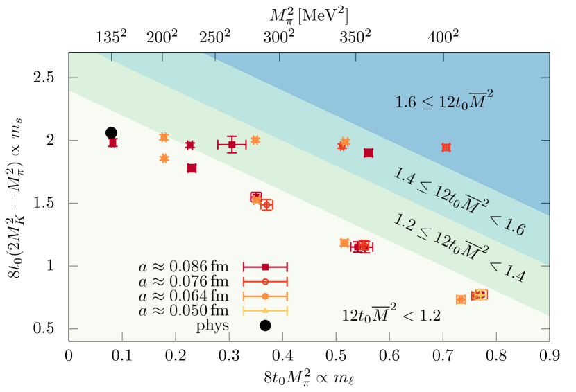
Figure 1: The positions of the analysed CLS ensembles in the quark mass plane. Both trajectories intersect close to the physical point (black circle) and one ensemble (D150) is very close to that point. Shading represent cuts on the average pseudoscalar meson mass $12t_{0}\overline{M}^{2}=4t_{0}(2M_{K}^{2}+M_{\pi}^{2})$ that we impose during our chiral extrapolation procedure. Symbols encode the four lattice spacings.

We employ twenty-one CLS gauge ensembles generated with $N_{f}=2+1$ non-perturbatively $\mathcal{O}(a)$ improved Wilson fermions. For details, see [28]. Two mass trajectories were realized that both lead to the physical point. Along one trajectory the average quark mass is held fixed [28], along the other trajectory the strange quark mass is kept approximately constant [29]. All ensembles have large volumes with $L_{s}>2.2\,{\rm fm}$ and $L_{s}M_{\pi}>4$ on most of them. To have full control over the continuum limit extrapolation, we incorporate four lattice spacings, $0.050\,{\rm fm}\leq a\leq 0.086\,{\rm fm}$.

On every configuration, we compute a matrix of correlation functions,

$$C_{ij}(\vec{p},t)=\frac{1}{N_{t_{\mathrm{in}}}}\sum_{t_{\mathrm{in}}}\left\langle\Omega\left|\mathcal{B}_{i}(\vec{p},t+t_{\mathrm{in}})\mathcal{B}^{\dagger}_{j}(-\vec{p},t_{\mathrm{in}})\right|\Omega\right\rangle,$$ (1)

where $|\Omega\rangle$ is the vacuum and $N_{t_{\mathrm{in}}}$ denotes the number of source time slices that we average over. We mostly use open boundary conditions and in these cases we sum only over the bulk of the lattice where boundary effects are negligible.

The interpolators $\mathcal{B}_{i}$ are octet and singlet combinations of spatially smeared pseudoscalar quark-antiquark interpolating operators,

$$\mathcal{P}^{8} =\frac{1}{\sqrt{6}}\left(\mathcal{P}^{u}+\mathcal{P}^{d}-2\mathcal{P}^{s}\right)=\frac{1}{\sqrt{3}}\mathcal{P}^{\ell}-\sqrt{\frac{2}{3}}\mathcal{P}^{s},$$ (2)

$$\mathcal{P}^{0} =\frac{1}{\sqrt{3}}\left(\mathcal{P}^{u}+\mathcal{P}^{d}+\mathcal{P}^{s}\right)=\sqrt{\frac{2}{3}}\mathcal{P}^{\ell}+\frac{1}{\sqrt{3}}\mathcal{P}^{s}$$ (3)

with $\mathcal{P}^{q}=\overline{q}\gamma_{5}q$, $q\in\{u,d,s\}$ and $\mathcal{P}^{\ell}=\frac{1}{\sqrt{2}}\left(\overline{u}\gamma_{5}u+\overline{d}\gamma_{5}d\right)$. To extract matrix elements, we also use corresponding (partially $\mathcal{O}(a)$-improved) local axialvector $A_{\mu}^{a}=\bar{\psi}t^{a}\gamma_{\mu}\gamma_{5}\psi+ac_{A}\partial_{\mu}P^{a}$ ($\bar{\psi}=(\bar{u},\bar{d},\bar{s})$), and pseudoscalar currents $P^{a}=\bar{\psi}t^{a}\gamma_{5}\psi$ at the sink. Note that this normalization differs from that of eqs. (2)–(3) by a factor $1/\sqrt{2}$. The disconnected loops entering the correlators are estimated using 96 stochastic sources. To keep near-neighbour noise under control we subtract the (for our action and operator) maximum possible number of terms of the hopping parameter expansion [30] from the propagator and place the stochastic sources at every fourth timeslice (dilution, partitioning [31]) at a time. This corresponds to about 300 to 600 thousand solutions of the Wilson-Dirac equation per ensemble. For the extended interpolators, we employ two different levels of smearing. The matrix of correlators is usually built from $\mathcal{B}_{i}\in\{\mathcal{P}^{\ell},\mathcal{P}^{s},\mathcal{P}^{8}\}$ at two different smearing levels, except at the symmetric $m_{s}=m_{\ell}$ point, where the Wick contraction between singlet and octet currents vanishes and yields a block-diagonal matrix. This enables us to split the problem into two parts and to analyse pure octet and singlet correlation matrices separately.

Instead of solving the generalized eigenvalue problem [32, 33], we directly fit to the Euclidean time derivative to improve the signal [34, 35],

$$\partial_{t}C(t)\sim Z\left(\partial_{t}D(t)\right)Z^{\intercal},$$ (4)

where $\partial_{t}C(t)=\left(C(t+a)-C(t-a)\right)/(2a)$ is the symmetric discretized derivative and

$$\partial_{t}D(t)=-\mathrm{diag}\left[E_{n}\exp\left(-E_{n}t\right)\right]$$ (5)

for open boundaries. For periodic boundaries the back-propagating part is taken into account. All time-dependence is contained in the diagonal matrix of eigenvalues, $D$, while the amplitudes are encoded in the matrix $Z_{in}=\langle\mathcal{B}_{i}|n\rangle/\sqrt{2E_{n}V_{3}}$, where $|n\rangle$ is the eigenstate corresponding to the $n$-th energy level $E_{n}$ and $V_{3}$ is the spatial volume.

To improve the stability of the multi-exponential fit and to increase the sensitivity to the $\eta^{\prime}$ state, we include a generalized version of the effective mass into our fully correlated fit,

$$\partial_{t}\log C(t)= (\partial_{t}C(t))C^{-1}(t)\approx\left({Z}\partial_{t}{D}(t){Z}^{\intercal}\right)\left({Z}{D}(t){Z}^{\intercal}\right)^{-1}=-Z\,\mathrm{diag}_{n=0}^{N-1}(E_{n})\,Z^{-1},$$ (6)

which is constant in time (up to excited states corrections and statistical noise). We further improve the signal by including data at the first non-zero momentum into our combined fit, employing the continuum dispersion relation, $E_{n}(\vec{p})=\sqrt{M_{n}^{2}+a^{2}\vec{p}^{2}}$. We show the results on the individual ensembles together with a comparison to other lattice determinations in fig. 2

Figure 2: Recent $N_{f}=2+1(+1)$ lattice results for the masses of the $\eta$ and $\eta^{\prime}$ mesons. Most points have been simulated at approximately physical strange quark masses (open symbols), whereas in this work we also include an additional trajectory along which the average of the quark masses is kept constant (filled symbols). The three sets of points in the shaded regions left of the physical point (dashed line) correspond to the continuum and chirally extrapolated results of JLQCD [20] (who do not give an estimate of $M_{\eta}$), ETMC [26] and this work.

Having extracted energies and eigenstates of the $\eta$ and $\eta^{\prime}$ mesons, we are in a position to compute decay constants,

$$Z_{A}^{a}(a,\mu)\left\langle\Omega\left|A_{\mu}^{a}\right|\mathcal{M}(p)\right\rangle=iF^{a}_{\mathcal{M}}p_{\mu},$$ (7)

where $Z_{A}^{a}(\mu)$ is a renormalization factor. While $Z_{A}=Z_{A}^{8}$ is scale-independent, the singlet renormalization factor $Z_{A}^{s}(\mu)=Z_{A}^{0}(\mu)$ depends on the scale. The normalization $A_{\mu}^{a}=\bar{\psi}t^{a}\gamma_{\mu}\gamma_{5}\psi$ that we adopt corresponds to $F_{\pi^{0}}^{3}\approx 92\,$MeV. Note that there are two decay constants each for $\mathcal{M}\in\{\eta,\eta^{\prime}\}$: singlet ($a=0$) and octet ($a=8$). These are often parametrized in terms of two decay constant parameters $F^{0}$ and $F^{8}$ and two angles $\theta_{8}$ and $\theta_{0}$,

$$\begin{pmatrix}F_{\eta}^{8}&F_{\eta}^{0}\\ F_{\eta^{\prime}}^{8}&F_{\eta^{\prime}}^{0}\end{pmatrix}=\begin{pmatrix}F^{8}\cos\theta_{8}&-F^{0}\sin\theta_{0}\\ F^{8}\sin\theta_{8}&F^{0}\cos\theta_{0}\end{pmatrix}.$$ (8)

3 Physical point results for masses and decay constants

We perform a combined continuum limit and chiral extrapolation of both masses and the four decay constants, employing large-$N_{c}$ ChPT to NLO [36, 6]. This allows us to describe the quark mass dependence of these six observables in the continuum theory by a common set of six low-energy constants: the pion decay constant in the chiral limit, $F$, the large-$N_{c}$ versions of the familiar SU(3) LECs $L_{5}$ and $L_{8}$, as well as the LECs $M_{0}^{2}$, $\Lambda_{1}$ and $\Lambda_{2}$. The singlet mass $M_{0}(\mu)$ in the chiral limit is related to the topological susceptibility and depends on the QCD scale $\mu$. The remaining two OZI suppressed parameters $\Lambda_{1}(\mu)$ and $\Lambda_{2}(\mu)$ depend on the QCD renormalization scale too. This is due to the anomalous dimension of the singlet axialvector current. Since this vanishes at leading order, in the limit $\mu\rightarrow\infty$, the singlet renormalization factor $Z_{A}^{s}(\infty)$ remains finite and we perform our fits in that limit. If needed, the results can then be evolved back to lower energy scales. The difference between the singlet and the non-singlet renormalization factors for our lattice action is known perturbatively to two loops [37] and we use the non-perturbatively determined $Z_{A}$ [38] for the non-singlet current. Note that chiral logs only appear at NNLO in the large-$N_{c}$ ChPT power counting. Therefore, all NLO LECs are independent of the ChPT renormalization scale (but some depend on the QCD scale $\mu$).

In order to account for the lattice spacing dependence, we include parameterizations of three unknown linear improvement coefficients of the singlet and one of the octet current into our fit, while setting the remaining coefficients to their literature values [39]. In this way, full $\mathcal{O}(a)$ improvement is achieved with four additional fit parameters. We then add systematically $\mathcal{O}(a^{2}\Lambda^{2})$, $\mathcal{O}(a^{2}\Lambda(2m_{\ell}+m_{s}))$ and $\mathcal{O}(a^{2}\Lambda(m_{s}-m_{\ell}))$ terms to all observables and subsequently remove those that we cannot determine.

In this way, we carried out 17 different fits that all gave acceptable $\chi^{2}$ values. The systematic error associated with the continuum limit is computed from the central 68.5 % range of the scatter of these results. On every ensemble we take into account the correlations between the non-singlet quark masses (the arguments of the fit functions) and the observables using Orear’s method [40]. The best fit gives $\chi^{2}/N_{\rm df}\approx 1.47$ and we quote its result as central values. We plot all our results at non-physical quark masses and their extrapolations to the physical point in fig. 3.

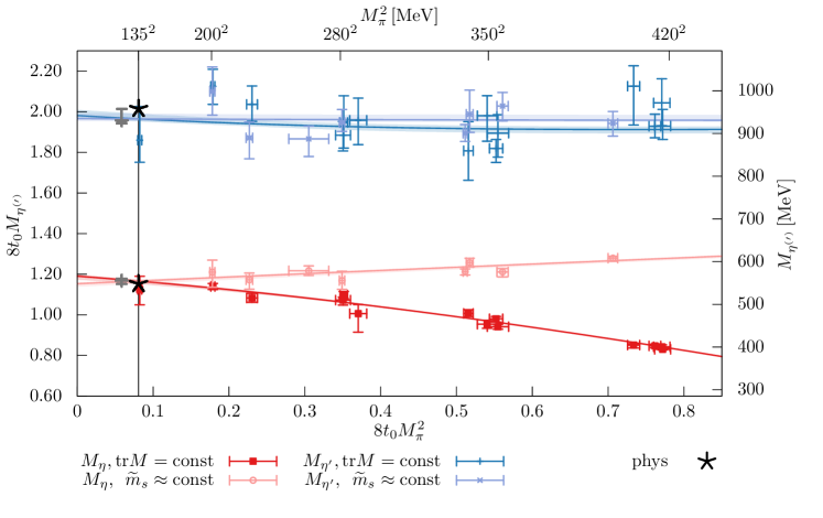
Figure 3: Chiral extrapolation of the masses (top) and decay constants (bottom) as a function of $M_{\pi}^{2}$. The two analyzed trajectories meet at the physical point.

To estimate the systematic uncertainties from the chiral extrapolation we follow a similar approach and remove ensembles with large average squared non-singlet pseudoscalar masses $12t_{0}\overline{M}^{2}=4t_{0}(2M_{K}^{2}+M_{\pi}^{2})$, see fig. 1. We also repeat fits for different initial energy scales $\mu_{0}\in\{a^{-1}/2,a^{-1},2a^{-1}\}$ from which we start the evolution of the scale-dependent singlet renormalization factor to $\mu=\infty$.

	no priors	exp. masses as priors
$L_{5}$	$\phantom{-}1.58\left(\begin{subarray}{c}17\\ 7\end{subarray}\right)_{\mathrm{stat}}\left(\begin{subarray}{c}0\\ 22\end{subarray}\right)_{a}\left(\begin{subarray}{c}20\\ 9\end{subarray}\right)_{\chi}\cdot 10^{-3}$	$\phantom{-}1.66\left(\begin{subarray}{c}12\\ 9\end{subarray}\right)_{\mathrm{stat}}\left(\begin{subarray}{c}0\\ 26\end{subarray}\right)_{a}\left(\begin{subarray}{c}13\\ 8\end{subarray}\right)_{\chi}\cdot 10^{-3}$
$L_{8}$	$\phantom{-}0.96\left(\begin{subarray}{c}15\\ 6\end{subarray}\right)_{\mathrm{stat}}\left(\begin{subarray}{c}0\\ 14\end{subarray}\right)_{a}\left(\begin{subarray}{c}16\\ 7\end{subarray}\right)_{\chi}\cdot 10^{-3}$	$\phantom{-}1.08\left(\begin{subarray}{c}11\\ 6\end{subarray}\right)_{\mathrm{stat}}\left(\begin{subarray}{c}0\\ 12\end{subarray}\right)_{a}\left(\begin{subarray}{c}3\\ 10\end{subarray}\right)_{\chi}\cdot 10^{-3}$
$M_{0}(\mu=\infty)$	$\phantom{-}1.67\left(\begin{subarray}{c}2\\ 6\end{subarray}\right)_{\mathrm{stat}}\left(\begin{subarray}{c}1\\ 2\end{subarray}\right)_{a}\left(\begin{subarray}{c}0\\ 1\end{subarray}\right)_{\chi}\left(\begin{subarray}{c}3\\ 2\end{subarray}\right)_{\mathrm{renorm}}\left(8t_{0}^{\chi}\right)^{-1/2}$	$\phantom{-}1.62\left(\begin{subarray}{c}2\\ 4\end{subarray}\right)_{\mathrm{stat}}\left(\begin{subarray}{c}3\\ 1\end{subarray}\right)_{a}\left(\begin{subarray}{c}3\\ 0\end{subarray}\right)_{\chi}\left(\begin{subarray}{c}2\\ 1\end{subarray}\right)_{\mathrm{renorm}}\left(8t_{0}^{\chi}\right)^{-1/2}$
	$=785\left(\begin{subarray}{c}9\\ 28\end{subarray}\right)_{\mathrm{stat}}\left(\begin{subarray}{c}15\\ 14\end{subarray}\right)_{\mathrm{syst}}(12)_{t_{0}}\,\mathrm{MeV}$	$=761\left(\begin{subarray}{c}13\\ 21\end{subarray}\right)_{\mathrm{stat}}\left(\begin{subarray}{c}18\\ 11\end{subarray}\right)_{\mathrm{syst}}(11)_{t_{0}}\,\mathrm{MeV}$
$F$	$\phantom{-}0.1890\left(\begin{subarray}{c}27\\ 37\end{subarray}\right)_{\mathrm{stat}}\left(\begin{subarray}{c}36\\ 0\end{subarray}\right)_{a}\left(\begin{subarray}{c}21\\ 38\end{subarray}\right)_{\chi}\left(8t_{0}^{\chi}\right)^{-1/2}$	$\phantom{-}0.1866\left(\begin{subarray}{c}26\\ 29\end{subarray}\right)_{\mathrm{stat}}\left(\begin{subarray}{c}54\\ 0\end{subarray}\right)_{a}\left(\begin{subarray}{c}19\\ 16\end{subarray}\right)_{\chi}\left(8t_{0}^{\chi}\right)^{-1/2}$
	$=88.83\left(\begin{subarray}{c}1.27\\ 1.74\end{subarray}\right)_{\mathrm{stat}}\left(\begin{subarray}{c}1.96\\ 1.79\end{subarray}\right)_{\mathrm{syst}}(1.32)_{t_{0}}\,\mathrm{MeV}$	$=87.71\left(\begin{subarray}{c}1.44\\ 1.57\end{subarray}\right)_{\mathrm{stat}}\left(\begin{subarray}{c}2.69\\ 81\end{subarray}\right)_{\mathrm{syst}}(1.31)_{t_{0}}\,\mathrm{MeV}$
$\Lambda_{1}(\mu=\infty)$	$-0.22\left(\begin{subarray}{c}1\\ 5\end{subarray}\right)_{\mathrm{stat}}\left(\begin{subarray}{c}0\\ 3\end{subarray}\right)_{a}\left(\begin{subarray}{c}0\\ 3\end{subarray}\right)_{\chi}\left(\begin{subarray}{c}6\\ 3\end{subarray}\right)_{\mathrm{renorm}}$	$-0.25\left(\begin{subarray}{c}1\\ 4\end{subarray}\right)_{\mathrm{stat}}\left(\begin{subarray}{c}3\\ 1\end{subarray}\right)_{a}\left(\begin{subarray}{c}1\\ 1\end{subarray}\right)_{\chi}\left(\begin{subarray}{c}5\\ 2\end{subarray}\right)_{\mathrm{renorm}}$
$\Lambda_{2}(\mu=\infty)$	$-0.1\left(\begin{subarray}{c}8\\ 4\end{subarray}\right)_{\mathrm{stat}}\left(\begin{subarray}{c}0\\ 10\end{subarray}\right)_{a}\left(\begin{subarray}{c}14\\ 8\end{subarray}\right)_{\chi}\left(\begin{subarray}{c}5\\ 3\end{subarray}\right)_{\mathrm{renorm}}$	$\phantom{-}0.11\left(\begin{subarray}{c}5\\ 5\end{subarray}\right)_{\mathrm{stat}}\left(\begin{subarray}{c}0\\ 9\end{subarray}\right)_{a}\left(\begin{subarray}{c}6\\ 5\end{subarray}\right)_{\chi}\left(\begin{subarray}{c}3\\ 2\end{subarray}\right)_{\mathrm{renorm}}$

Table 1: Large-$N_{c}$ LECs parametrizing the continuum limit of our results on the masses and decay constants. The left column is obtained from a unconstrained but fully correlated fit to all 21 ensembles. The right column is a fit to the same data but adding the physical masses (11) as a prior and gives very similar results. The conversion to physical unit was done using $(8t_{0}^{\chi})^{-1/2}=470(7)\,\mathrm{MeV}$ in the chiral limit [28, 41, 27].

Our central fit is parameterized in the continuum by the LECs listed in the left column of tab. 1 and yields for the masses at the physical point,

$$M_{\eta} =1.168\left(\begin{subarray}{c}8\\ 14\end{subarray}\right)_{\mathrm{stat}}\left(\begin{subarray}{c}1\\ 0\end{subarray}\right)_{a}\left(\begin{subarray}{c}5\\ 6\end{subarray}\right)_{\chi}(8t_{0}^{\rm ph})^{-1/2}=554.7\left(\begin{subarray}{c}4.0\\ 6.6\end{subarray}\right)_{\mathrm{stat}}\left(\begin{subarray}{c}2.4\\ 2.7\end{subarray}\right)_{\mathrm{syst}}(7.0)_{t_{0}}\,\mathrm{MeV}\quad\text{and}$$ (9)

$$M_{\eta^{\prime}} =1.958\left(\begin{subarray}{c}27\\ 13\end{subarray}\right)_{\mathrm{stat}}\left(\begin{subarray}{c}0\\ 6\end{subarray}\right)_{a}\left(\begin{subarray}{c}48\\ 3\end{subarray}\right)_{\chi}(8t_{0}^{\rm ph})^{-1/2}=929.9\left(\begin{subarray}{c}12.9\\ 6.0\end{subarray}\right)_{\mathrm{stat}}\left(\begin{subarray}{c}22.9\\ 3.3\end{subarray}\right)_{\mathrm{syst}}(11.7)_{t_{0}}\,\mathrm{MeV},$$ (10)

using the Wilson flow scale at the physical point $(8t_{0}^{\rm ph})^{-1/2}=475(6)\,\mathrm{MeV}$ [42] to convert to physical units. We find reasonably good agreement when comparing these results of $N_{f}=2+1$ QCD with the known experimental masses,

$$\text{PDG\,\cite[cite]{[\@@bibref{Number}{PDG}{}{}]}}:\qquad M^{\mathrm{ph}}_{\eta}=547.862(17)\,\mathrm{MeV}\quad\text{and}\quad M^{\mathrm{ph}}_{\eta^{\prime}}=957.78(6)\,\mathrm{MeV}.$$ (11)

The masses are 0.7 standard errors above and one standard error below the experimental values for the $\eta$ and $\eta^{\prime}$, respectively. We also carry out a second fit incorporating the knowledge of the physical masses by adding them as priors to the $\chi^{2}$ function and obtain similar results for the LECs listed in the right column of tab. 1. Using this second set of LECs, we obtain for the decay constants in the angle representation, eq. (8),

$$F^{8} =0.2421\left(\begin{subarray}{c}22\\ 26\end{subarray}\right)_{\mathrm{stat}}\left(\begin{subarray}{c}8\\ 50\end{subarray}\right)_{a}\left(\begin{subarray}{c}32\\ 12\end{subarray}\right)_{\chi}\,(8t_{0}^{\rm ph})^{-1/2}=115.0\left(\begin{subarray}{c}1.1\\ 1.2\end{subarray}\right)_{\mathrm{stat}}\left(\begin{subarray}{c}1.6\\ 2.4\end{subarray}\right)_{\mathrm{syst}}(1.5)_{t_{0}}\,\mathrm{MeV},$$ (12)

$$\theta_{8} =-0.450\left(\begin{subarray}{c}21\\ 36\end{subarray}\right)_{\mathrm{stat}}\left(\begin{subarray}{c}24\\ 0\end{subarray}\right)_{a}\left(\begin{subarray}{c}29\\ 0\end{subarray}\right)_{\chi}\left(\begin{subarray}{c}1\\ 5\end{subarray}\right)_{\mathrm{renorm}}=-25.8\left(\begin{subarray}{c}1.2\\ 2.1\end{subarray}\right)_{\mathrm{stat}}\left(\begin{subarray}{c}2.2\\ 0.3\end{subarray}\right)_{\mathrm{syst}}^{\circ},$$ (13)

$$F^{0}(\mu=2\,\mathrm{GeV}) =0.2108\left(\begin{subarray}{c}14\\ 40\end{subarray}\right)_{\mathrm{stat}}\left(\begin{subarray}{c}12\\ 25\end{subarray}\right)_{a}\left(\begin{subarray}{c}30\\ 8\end{subarray}\right)_{\chi}\left(\begin{subarray}{c}50\\ 26\end{subarray}\right)_{\mathrm{renorm}}\,(8t_{0}^{\rm ph})^{-1/2}$$

$$=100.1\left(\begin{subarray}{c}7\\ 1.9\end{subarray}\right)_{\mathrm{stat}}\left(\begin{subarray}{c}2.0\\ 2.7\end{subarray}\right)_{\mathrm{syst}}(1.3)_{t_{0}}\,\mathrm{MeV},$$ (14)

$$\theta_{0} =-0.141\left(\begin{subarray}{c}18\\ 20\end{subarray}\right)_{\mathrm{stat}}\left(\begin{subarray}{c}0\\ 27\end{subarray}\right)_{a}\left(\begin{subarray}{c}27\\ 0\end{subarray}\right)_{\chi}=-8.1\left(\begin{subarray}{c}1.0\\ 1.1\end{subarray}\right)_{\mathrm{stat}}\left(\begin{subarray}{c}1.5\\ 1.5\end{subarray}\right)_{\mathrm{syst}}^{\circ}.$$ (15)

In comparison to the frequently used flavour representation, the octet/singlet representation has the advantage that only the singlet decay constants depend on the renormalization scale. We refer to tabs. 24 and 25 of [27] for results at several scales and in different parameterizations.

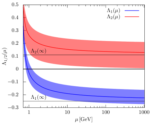
Figure 4: Scale dependence of the large-$N_{c}$ ChPT LECs $\Lambda_{1}$ and $\Lambda_{2}$.

The QCD scale-dependence cannot be determined from phenomenological fits to experimental low-energy data. Therefore, only scale-independent combinations of the large-$N_{c}$ ChPT LECs $M_{0}^{2},\Lambda_{1}$ and $\Lambda_{2}$ [4] are accessible, unless additional assumptions are made. The most prominent framework is the Feldmann-Kroll-Stech (FKS) model [5, 44, 45] which uses the fact that in the flavour basis the difference between the light and strange mixing angles is OZI suppressed and proportional to $\Lambda_{1}$. This reduces the number of independent parameters for the four decay constants to three, setting $\phi_{\ell}=\phi_{s}$ and assuming $\Lambda_{1}=0$. Our analysis shows that the latter approximation indeed holds at low energy scales ($\mu\approx 1\,\mathrm{GeV}$), see fig. 4, and that the FKS model works to a reasonable accuracy. Therefore, our results are in good agreement with [45] and many other phenomenological determinations.

4 Pseudoscalar states above the $\eta^{\prime}$

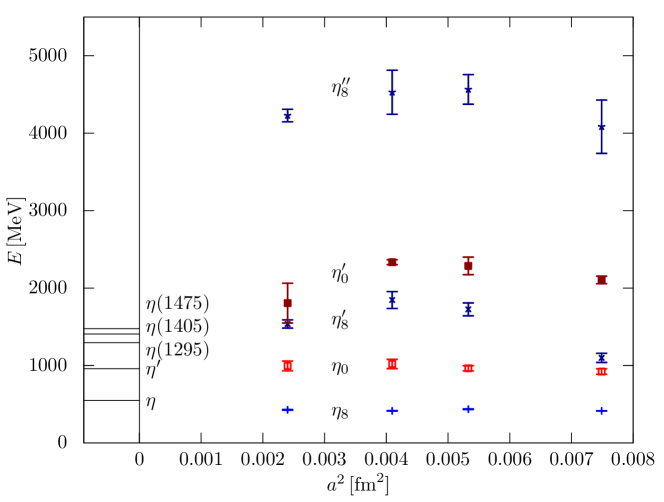
Figure 5: The octet (blue) and singlet (red) energy levels at the $m_{s}=m_{\ell}$ point versus the squared lattice spacing. For orientation also the experimental resonances (at physical quark masses) are shown.

We usually analyse a $3\times 3$ matrix of correlation functions to extract the lowest two energy levels, the $\eta$ and the $\eta^{\prime}$. The higher excitations are not resolved but effectively described by a third energy level. At the $N_{f}=3$ symmetric point the matrix of correlation functions is block diagonal regarding the singlet and octet sectors. Therefore, at this point, we can resolve higher excitations. In experiment several resonances with the same quantum numbers are relatively close to the $\eta^{\prime}$, namely the $\eta(1295)$, $\eta(1405)$ and the $\eta(1475)$. The first state decays mostly into $\eta\pi\pi$. This may indicate that the octet component dominates. In contrast, $\eta(1405)$ and $\eta(1475)$ decay into $K\bar{K}\pi$, $a_{0}\pi$ etc. The $\eta(1405)$ which, unlike the $\eta(1475)$, has not been observed to decay into $\gamma\gamma$ has even been postulated to be a glueball [46], however, unlike the $\eta(1475)$ and like the $\eta(1295)$, it also decays into $\eta\pi\pi$.

On our $m_{s}=m_{\ell}$ ensembles we use a $2\times 2$ matrix of smeared singlet interpolators for the $\eta^{\prime}=\eta_{0}$ and in case of the octet we include the local current in addition, resulting in a $3\times 3$ matrix. This enables us to determine the first excited singlet and the first two excited octet states, see fig. 5. At $a=0$ we have included the experimental spectrum for orientation. One should keep in mind, however, that this refers to the physical point and not to $m_{s}=m_{\ell}$. We observe large cutoff effects that have a similar shape for all the excited states. In contrast, for the ground states we are unable to resolve any lattice spacing dependence. The third octet state is around 4 GeV, indicating that the first excitation becomes the $\eta(1295)$ at the physical point and that the $\eta(1405)$ and $\eta(1475)$ may have large singlet components, although we are unable to resolve more than one singlet state within this energy region within our statistical accuracy.

5 Gluonic matrix elements

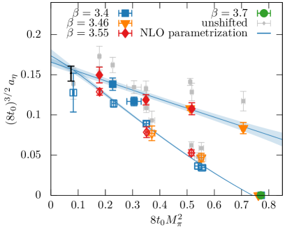
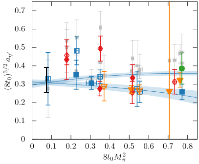
Figure 6: The anomalous gluonic matrix element $a_{\eta}$ (left) and $a_{\eta^{\prime}}$ (right) determined via the singlet AWI from fermionic matrix elements, eq. (18). The coloured points have been adjusted for lattice spacing effects, while the grey points indicate the unshifted data. The two curves correspond to the NLO large-$N_{c}$ ChPT parametrization derived in [27] for trajectories with a constant average quark mass and a constant strange quark mass. The black error bars indicate the final results at the physical point including statistical and systematic errors.

After constructing interpolators that create the $\eta$ and $\eta^{\prime}$ mesons, based on the overlap factors $Z_{in}$ of eq. (4), we may also compute local matrix elements other than the decay constants. The singlet axial Ward identity connects axial and pseudoscalar quark bilinear currents with the topological charge density $\omega(x)=-\tfrac{1}{32\pi^{2}}F_{\mu\nu}^{a}(x)\widetilde{F}_{\mu\nu}^{a}(x)$,

$$\partial_{\mu}\widehat{A}^{a}_{\mu}=\widehat{\left(\overline{\psi}\gamma_{5}\{M,t^{a}\}\psi\right)}+\sqrt{6}\delta^{a0}\widehat{\omega},$$ (16)

where $M=\mathrm{diag}(m_{\ell},m_{\ell},m_{s})$ is the quark mass matrix, $a\in\{0,\ldots,8\}$ labels the generators of U(3), $t^{a}=\lambda^{a}/2$ and $t^{0}=\mathds{1}/\sqrt{6}$. Hats denote renormalized quantities. For the determination of the topological charge density we evolve the gauge fields to a gradient flow time $\sqrt{8t}=\sqrt{8t_{0}^{*}}\approx 0.413\,\mathrm{fm}$. Under renormalization $\omega$ mixes with $\partial_{\mu}A_{\mu}^{0}$,

$$\hat{\omega}=Z_{\omega}\omega+Z_{\omega A}\partial_{\mu}A_{\mu}^{0},$$ (17)

and the renormalization factors are unknown. We therefore start by constructing the anomalous matrix elements $a_{\eta^{(\prime)}}=2\langle\Omega|\hat{\omega}|\eta^{(\prime)}\rangle$ by combining axialvector and pseudoscalar matrix elements,

$$a_{\mathcal{M}}(\mu)=\sqrt{\frac{2}{3}}Z_{A}^{s}(\mu)\partial_{\mu}\left\langle\Omega\left|A_{\mu}^{0}\right|\mathcal{M}\right\rangle+\frac{2\sqrt{2}}{\sqrt{3}}Z_{A}\left[\frac{\sqrt{2}}{3}\delta\widetilde{m}\left\langle\Omega\left|P^{8}\right|\mathcal{M}\right\rangle-r_{P}\overline{\widetilde{m}}\left\langle\Omega\left|P^{0}\right|\mathcal{M}\right\rangle\right].$$ (18)

The PCAC masses $\overline{\widetilde{m}}=(2\widetilde{m}_{\ell}+\widetilde{m}_{s})/3$ and $\delta\widetilde{m}=\widetilde{m}_{s}-\widetilde{m}_{\ell}$ are determined from the non-singlet PCAC relations (e.g., $a=1$ and $a=4$) and we set $r_{P}=Z_{P}^{s}/Z_{P}=1$ since the difference $Z_{P}^{s}-Z_{P}=\mathcal{O}(g^{6})$ for Wilson quarks. We then attempt a combined fit to the $a_{\eta}$ and $a_{\eta^{\prime}}$ data, again parameterizing all four additional unknown pseudoscalar $\mathcal{O}(a)$ improvement coefficients within the fit. We derived the full NLO ChPT continuum expression in [27]. To this order no LECs enter other than those that we already have determined above. In view of the limited statistical accuracy, we do not attempt to parameterize higher lattice artifacts and set priors on the six LEC, keeping them close to the central fit results in tab. 1. From this fit with $\chi^{2}/N_{\rm df}\approx 1.09$, we obtain at the physical point

$$a_{\eta}(\mu=\infty)=0.1564\left(\begin{subarray}{c}37\\ 63\end{subarray}\right)_{\rm stat}(45)_{\rm syst}(8t_{0}^{\rm ph})^{-3/2}=0.01676\left(\begin{subarray}{c}40\\ 67\end{subarray}\right)_{\rm stat}\left(48\right)_{\rm syst}\left(65\right)_{t_{0}}\,\mathrm{GeV}^{3},$$ (19)

$$a_{\eta^{\prime}}(\mu=\infty)=0.308\left(\begin{subarray}{c}16\\ 17\end{subarray}\right)_{\rm stat}(80)_{\rm syst}(8t_{0}^{\rm ph})^{-3/2}=0.0330\left(\begin{subarray}{c}18\\ 17\end{subarray}\right)_{\rm stat}\left(80\right)_{\rm syst}\left(16\right)_{t_{0}}\,\mathrm{GeV}^{3}.$$ (20)

The systematic error is taken as the difference between the results of this fit and the NLO prediction using the previously determined LECs alone. The fit and the physical point results are shown in fig. 6. Results at lower renormalization scales can be found in tab. 19 of [27].

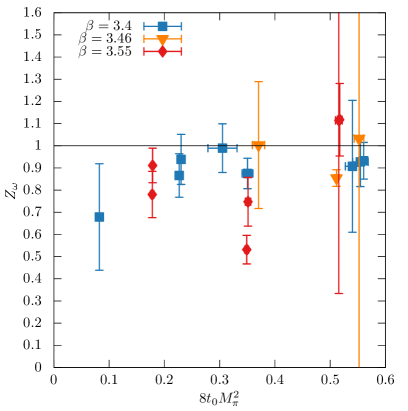
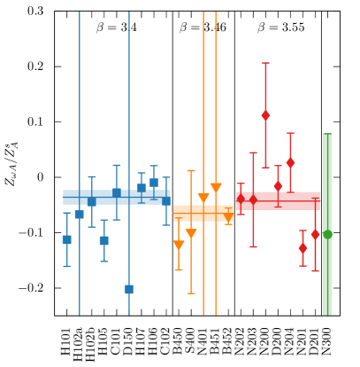
Figure 7: (Left) $Z_{\omega}$ from solving eq. (21). The $m_{s}=m_{\ell}$ points are not shown since in these cases $F_{\eta}^{0}=0$ and the equation system is singular. (Right) Values of $Z_{\omega A}/Z_{A}^{s}$ from solving eq. (21), assuming $Z_{\omega}=1$.

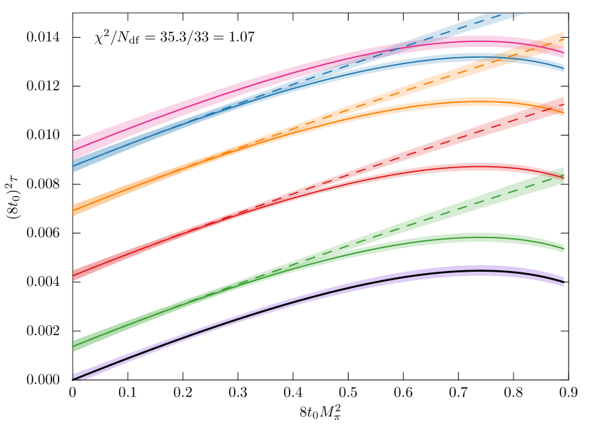
Figure 8: Topological susceptibility for many of the CLS ensembles described in [41]. Filled symbols mark ensembles that are simulated with a constant sum of quark masses (solid lines), open symbols correspond to ensembles with the strange quark mass fixed to approximately the physical value (dashed lines). Lines and shaded regions are the result of a fit to eq. (22), adding $a^{2}$, $a^{3}$ and $a^{4}$ coefficients. The continuum limit result (black lines) is very close to both the fit result at $\beta=3.85$ as well as the leading order expectation (grey lines), when using $\sqrt{8t_{0}}F=0.1866$, see tab. 1 and setting $Z_{\omega}=1$.

To establish the consistency between the above fermionic definition of the matrix elements $a_{\mathcal{M}}$ and a direct gluonic determination, we investigate the mixing under renormalization eq. (17). We start by solving the set of linear equations

$$a_{\mathcal{M}}(\mu)=2\,Z_{\omega}\langle\Omega|\omega|\mathcal{M}\rangle+2\frac{Z_{\omega A}}{Z_{A}^{s}}M_{\mathcal{M}}^{2}F_{\mathcal{M}}^{0}(\mu),$$ (21)

for the unknown renormalization factors using the fermionic definition of $a_{\mathcal{M}}$ for $\mathcal{M}=\eta$ and $\mathcal{M}=\eta^{\prime}$. The result for $Z_{\omega}$ is plotted on the left panel of fig. 7 and is consistent with $Z_{\omega}=1$, which we expect when using flowed gauge fields. We confirm this observation by fitting the topological susceptibility on many CLS ensembles to the leading order ChPT continuum expectation for the $N_{f}=2+1$ theory [1, 47],

$$\hat{\tau}=\frac{F^{2}}{2}\left(\frac{1}{2M_{K}^{2}-M_{\pi}^{2}}+\frac{2}{M_{\pi}^{2}}\right)^{-1},$$ (22)

where we parameterize the sizable cutoff effects with quadratic, cubic and quartic terms in the lattice spacing. Data and fit are shown in fig. 8. We obtain $F\sqrt{8t_{0}^{\chi}}/Z_{\omega}=0.190(13)$, which agrees with $F\sqrt{8t_{0}^{\chi}}=0.1866(48)$ from the parametrization of the masses and decay constants (see tab. 1) if we set $Z_{\omega}=1$, which demonstrates that indeed $Z_{\omega}\approx 1$ with the gradient flow definition of $\omega$.

Assuming $Z_{\omega}=1$ and using the fermionic definition of $a_{\mathcal{M}}$, we isolate the ratio $Z_{\omega A}/Z_{A}^{s}$ in eq. (21), that only depends on the coupling parameter but not on the scale. We plot this in the right panel of fig. 7. Using weighted averages for each lattice coupling, this determines the second renormalization factor and enables a comparison between the fermionic (eq. (18)) and gluonic (eq. (21)) definitions of the anomalous matrix elements, see the scatter plot fig. 9. We also show the anomalous matrix elements without taking the mixing into account ($Z_{\omega A}=0$). In this case, one would have underestimated $a_{\eta^{(\prime)}}$ by about 30%, using the gluonic definition.

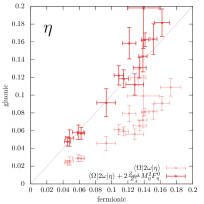
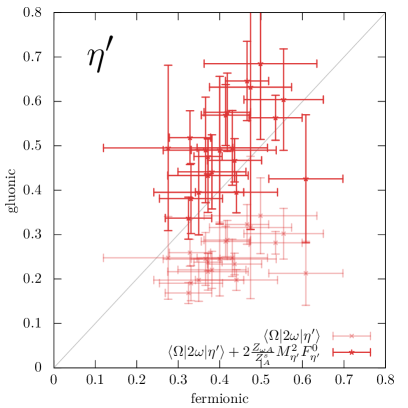
Figure 9: Scatter plot of the fermionic (eq. (18), horizontally) and gluonic (eq. (21), vertically) determinations of the gluonic matrix elements $a_{\eta^{(\prime)}}$. The mixing with the derivative of the axialvector current is non-negligible: the unrenormalized lattice matrix elements (pale red points) do not agree with the fermionic definition.

6 Summary

In these proceedings we summarized our computation of the masses, the complete set of decay constants and the anomalous matrix elements for the $\eta$ and $\eta^{\prime}$ states that we recently published in [27]. The interested reader is referred to that publication for more technical detail and comparison to literature values. The decay constants and anomalous matrix elements were determined for the first time from first principles. Our physical point extrapolation is facilitated by using twenty-one CLS ensembles on two mass trajectories and four lattice spacings. We employed NLO large-$N_{c}$ ChPT to describe the continuum limit mass dependence. The results are well parameterized by this ansatz, including the anomalous matrix elements and we determined all six NLO LECs. The scale dependence has been studied and shows that the FKS approximation [5, 44, 45] works surprisingly well at low energies, which is a consequence of $\Lambda_{1}(1\,\mathrm{GeV})\approx 0$. In addition to the already published results, we determined masses of higher excitations for $m_{\ell}=m_{s}$, see fig. 5. We found a very large mass for the second excited octet state while the first excited octet state has a smaller mass than the first excited singlet state.

Acknowledgments. This work was supported by the Deutsche Forschungsgemeinschaft (SFB/TRR-55 and FOR 2926) and the European Union’s Horizon 2020 research and innovation programme under the Marie Skłodowska-Curie grant agreement no. 813942 (ITN EuroPLEx) and grant agreement no. 824093 (STRONG-2020). We thank our colleagues in CLS [http://wiki-zeuthen.desy.de/CLS/CLS]. The authors gratefully acknowledge the Gauss Centre for Supercomputing (GCS) for providing computing time through the John von Neumann Institute for Computing (NIC) on JUQUEEN, JUWELS [48] and in particular JURECA-Booster [49] at Jülich Supercomputing Centre (JSC).

References

- [1] P. Di Vecchia and G. Veneziano, Chiral dynamics in the large limit, Nucl. Phys. B 171 (1980) 253.
- [2] K. Kawarabayashi and N. Ohta, The problem of in the large limit: Effective Lagrangian approach, Nucl. Phys. B 175 (1980) 477.
- [3] P. Di Vecchia, F. Nicodemi, R. Pettorino and G. Veneziano, Large , chiral approach to pseudoscalar masses, mixings and decays, Nucl. Phys. B 181 (1981) 318.
- [4] H. Leutwyler, On the expansion in chiral perturbation theory, Nucl. Phys. B Proc. Suppl. 64 (1998) 223 [hep-ph/9709408].
- [5] T. Feldmann, P. Kroll and B. Stech, Mixing and decay constants of pseudoscalar mesons, Phys. Rev. D 58 (1998) 114006 [hep-ph/9802409].
- [6] P. Bickert, P. Masjuan and S. Scherer, - Mixing in Large- Chiral Perturbation Theory, Phys. Rev. D 95 (2017) 054023 [1612.05473].
- [7] Y. Kuramashi, M. Fukugita, H. Mino, M. Okawa and A. Ukawa, meson mass in lattice QCD, Phys. Rev. Lett. 72 (1994) 3448.
- [8] L. Venkataraman and G. Kilcup, The meson with staggered fermions, hep-lat/9711006.
- [9] W.A. Bardeen, A. Duncan, E. Eichten and H. Thacker, Anomalous chiral behavior in quenched lattice QCD, Phys. Rev. D 62 (2000) 114505 [hep-lat/0007010].
- [10] TL collaboration, Flavor singlet pseudoscalar masses in QCD, Phys. Rev. D 63 (2001) 074503 [hep-lat/0010005].
- [11] UKQCD collaboration, The and ’ mesons in QCD, Phys. Lett. B 491 (2000) 123 [hep-lat/0006020].
- [12] SESAM, TL collaboration, Quark mass effects on the topological susceptibility in QCD, Phys. Rev. D 64 (2001) 054502 [hep-lat/0102002].
- [13] CP-PACS collaboration, Flavor singlet meson mass in the continuum limit in two flavor lattice QCD, Phys. Rev. D 67 (2003) 074503 [hep-lat/0211040].
- [14] K. Hashimoto and T. Izubuchi, meson from two flavor dynamical domain wall fermions, Prog. Theor. Phys. 119 (2008) 599 [0803.0186].
- [15] ETM collaboration, The meson from lattice QCD, Eur. Phys. J. C 58 (2008) 261 [0804.3871].
- [16] N.H. Christ, C. Dawson, T. Izubuchi, C. Jung, Q. Liu, R.D. Mawhinney et al., The and mesons from Lattice QCD, Phys. Rev. Lett. 105 (2010) 241601 [1002.2999].
- [17] J.J. Dudek, R.G. Edwards, B. Joo, M.J. Peardon, D.G. Richards and C.E. Thomas, Isoscalar meson spectroscopy from lattice QCD, Phys. Rev. D 83 (2011) 111502 [1102.4299].
- [18] UKQCD collaboration, A study of the and mesons with improved staggered fermions, Phys. Rev. D 86 (2012) 014504 [1112.4384].
- [19] G.S. Bali, S. Collins, S. Dürr and I. Kanamori, semileptonic decay form factors with disconnected quark loop contributions, Phys. Rev. D 91 (2015) 014503 [1406.5449].
- [20] JLQCD collaboration, meson mass from topological charge density correlator in QCD, Phys. Rev. D 92 (2015) 111501 [1509.00944].
- [21] W. Sun, L.-C. Gui, Y. Chen, M. Gong, C. Liu, Y.-B. Liu et al., Glueball spectrum from lattice QCD study on anisotropic lattices, Chin. Phys. C 42 (2018) 093103 [1702.08174].
- [22] P. Dimopoulos et al., Topological susceptibility and meson mass from lattice QCD at the physical point, Phys. Rev. D 99 (2019) 034511 [1812.08787].
- [23] CSSM/QCDSF/UKQCD collaboration, State mixing and masses of the , and mesons from lattice QCD+QED, 2110.11533.
- [24] ETM collaboration, and mesons from twisted mass lattice QCD, JHEP 11 (2012) 048 [1206.6719].
- [25] ETM collaboration, and mixing from Lattice QCD, Phys. Rev. Lett. 111 (2013) 181602 [1310.1207].
- [26] ETM collaboration, Flavor-singlet meson decay constants from twisted mass lattice QCD, Phys. Rev. D 97 (2018) 054508 [1710.07986].
- [27] RQCD collaboration, Masses and decay constants of the and ’ mesons from lattice QCD, JHEP 08 (2021) 137 [2106.05398].
- [28] M. Bruno et al., Simulation of QCD with N 2 1 flavors of non-perturbatively improved Wilson fermions, JHEP 02 (2015) 043 [1411.3982].
- [29] RQCD collaboration, Lattice simulations with improved Wilson fermions at a fixed strange quark mass, Phys. Rev. D 94 (2016) 074501 [1606.09039].
- [30] G.S. Bali, S. Collins and A. Schäfer, Effective noise reduction techniques for disconnected loops in Lattice QCD, Comput. Phys. Commun. 181 (2010) 1570 [0910.3970].
- [31] S. Bernardson, P. McCarty and C. Thron, Monte Carlo methods for estimating linear combinations of inverse matrix entries in lattice QCD, Comput. Phys. Commun. 78 (1993) 256.
- [32] C. Michael, Adjoint sources in lattice gauge theory, Nucl. Phys. B 259 (1985) 58.
- [33] M. Lüscher and U. Wolff, How to calculate the elastic scattering matrix in two-dimensional quantum field theories by numerical simulation, Nucl. Phys. B 339 (1990) 222.
- [34] X. Feng, K. Jansen and D.B. Renner, The scattering length from maximally twisted mass lattice QCD, Phys. Lett. B 684 (2010) 268 [0909.3255].
- [35] T. Umeda, A constant contribution in meson correlators at finite temperature, Phys. Rev. D 75 (2007) 094502 [hep-lat/0701005].
- [36] J. Gasser and H. Leutwyler, Chiral Perturbation Theory: Expansions in the mass of the strange quark, Nucl. Phys. B 250 (1985) 465.
- [37] M. Constantinou, M. Hadjiantonis, H. Panagopoulos and G. Spanoudes, Singlet versus nonsinglet perturbative renormalization of fermion bilinears, Phys. Rev. D 94 (2016) 114513 [1610.06744].
- [38] J. Bulava, M. Della Morte, J. Heitger and C. Wittemeier, Nonperturbative renormalization of the axial current in lattice QCD with Wilson fermions and a tree-level improved gauge action, Phys. Rev. D 93 (2016) 114513 [1604.05827].
- [39] G.S. Bali, K.G. Chetyrkin, P. Korcyl and J. Simeth, Non-perturbative determination of quark-mass independent improvement coefficients in lattice QCD, in preparation (2021) .
- [40] J. Orear, Least squares when both variables have uncertainties, Am. J. Phys. 50 (1982) 912.
- [41] RQCD collaboration, Scale setting and the light hadron spectrum in QCD with Wilson fermions, in preparation .
- [42] M. Bruno, T. Korzec and S. Schaefer, Setting the scale for the CLS flavor ensembles, Phys. Rev. D 95 (2017) 074504 [1608.08900].
- [43] Particle Data Group collaboration, Review of Particle Physics, PTEP 2020 (2020) 083C01.
- [44] T. Feldmann, P. Kroll and B. Stech, Mixing and decay constants of pseudoscalar mesons: The sequel, Phys. Lett. B 449 (1999) 339 [hep-ph/9812269].
- [45] T. Feldmann, Quark structure of pseudoscalar mesons, Int. J. Mod. Phys. A 15 (2000) 159 [hep-ph/9907491].
- [46] H.-Y. Cheng, H.-n. Li and K.-F. Liu, Pseudoscalar glueball mass from mixing, Phys. Rev. D 79 (2009) 014024 [0811.2577].
- [47] H. Leutwyler and A.V. Smilga, Spectrum of Dirac operator and role of winding number in QCD, Phys. Rev. D 46 (1992) 5607.
- [48] Jülich Supercomputing Centre, JUWELS: Modular Tier-0/1 Supercomputer at the Jülich Supercomputing Centre, Journal of Large-Scale Research Facilities 5 (2019) A135.
- [49] Jülich Supercomputing Centre, JURECA: Modular supercomputer at Jülich Supercomputing Centre, Journal of Large-Scale Research Facilities 4 (2018) A132.