Parameter-robust methods for the Biot-Stokes interfacial coupling without Lagrange multipliers

Abstract

In this paper we advance the analysis of discretizations for a fluid-structure interaction model of the monolithic coupling between the free flow of a viscous Newtonian fluid and a deformable porous medium separated by an interface. A five-field mixed-primal finite element scheme is proposed solving for Stokes velocity-pressure and Biot displacement-total pressure-fluid pressure. Adequate inf-sup conditions are derived, and one of the distinctive features of the formulation is that its stability is established robustly in all material parameters. We propose robust preconditioners for this perturbed saddle-point problem using appropriately weighted operators in fractional Sobolev and metric spaces at the interface. The performance is corroborated by several test cases, including the application to interfacial flow in the brain.

1 Introduction

1.1 Scope

We address the construction of appropriate monolithic solvers for multiphysics fluid-poromechanical couplings interacting through an interface. Particular attention is payed to tracking parameter dependence of the continuous and discrete formulations so that the resulting numerical methods are robust with respect to typical scales in material constants spanning over many orders of magnitude. We adopt a multi-domain approach, where appropriate conditions for the coupling through the shared interface need to be imposed. We use the conditions proposed in [1] (although, other forms and dedicated phenomena could be incorporated without much effort, such as fluid entry resistance [2, 3]). The recent literature contains various numerical methods for (Navier-)Stokes/Biot interface formulations including mixed, double mixed, monolithic, segregated, conforming, non-conforming, and DG discretizations [4, 5, 6, 7, 8, 9, 10, 11, 12, 13, 14, 15].

In [12, 16] (and starting from the Biot-Stokes equations advanced in [5, 17]) the authors rewrite the poroelasticity equations using displacement, fluid pressure and total pressure (also as in the poromechanics formulations from [18, 19, 20]). Since fluid pressure in the poroelastic domain has sufficient regularity, no Lagrange multipliers are needed to enforce the coupling conditions, which resembles the different formulations for Stokes-Darcy advanced in [21, 22, 23, 24]. Another advantage of the three-field Biot formulation is its robustness with respect to the Lamé constants of the poroelastic structure. This robustness is of particular importance when we test the flow response to changes in the material properties of the skeleton and when the solid is nearly incompressible. The work [12] focuses on the stability analysis and its precise implications on the asymptotics of the interface conditions when the permeability depends on porosity heterogeneity, whereas [16] addresses the stability of the semi- and fully discrete problems, and the application to interfacial flow in the eye. Here, we extend these works by concentrating on deriving robust stability, on designing efficient block preconditioners (robust with respect to all material parameters) following the general theoretical formalism from [25], and on the simulation of free flow interacting with interstitial flow in the brain. In such a context (and in the wider class of problems we consider in this paper), tissue permeability is of the order of 10^-15m², and the incorporation of tangential interface transmission conditions usually involves terms that scale inversely proportional to the square root of permeability. Moreover, the solid is nearly incompressible, making the first Lamé parameter significantly larger than the other mechanical parameters and exhibiting volumetric locking for some types of displacement-based formulations. Other flow regimes that are challenging include low-storage cases [26]. It is then important that the stability and convergence of the numerical approximations are preserved within the parameter ranges of interest.

Here we follow [27, 28, 20, 29] and use parameter-weighted norms to achieve robustness. However, as we will see, combining proper preconditioners for Stokes and Biot single-physics problems is not sufficient for the interface coupled problem. In fact, the condition number of the preconditioned system, although robust in mesh size, grows like the square root of the ratio between fluid viscosity and permeability. This phenomenon is demonstrated in Example 2.1, below. That is, the efficiency of seemingly natural preconditioners varies with the material parameters. In order to regain stability with respect to all parameters, we include both an additional fractional term involving the pressure and a metric term coupling the tangential fluid velocity and solid displacement at the interface, hereby increasing the regularity at the interface in a proper parameter dependent manner. This strategy draws inspiration from similar approaches employed in the design of robust solvers for Darcy and Stokes-Darcy couplings [30, 21, 23].

1.2 Outline

We have organised the contents of this paper in the following manner. The remainder of this section contains preliminaries on notation and functional spaces to be used throughout the manuscript. Section 2 outlines the main details of the balance equations, stating typical interfacial and boundary conditions, and restricting the discussion to the steady Biot-Stokes coupled problem. There we also include the weak formulation and demonstrate that simple diagonal preconditioners based on standard norms do not lead to robustness over the whole parameter range. This issue is addressed in Section 3 where we show well-posedness of the system using a global inf-sup argument with parameter weighted operators in fractional spaces, which in turn assist in the design of robust solvers by operator preconditioning. Section 4 discusses finite element discretization of the coupled problem using both conforming and non-conforming elements; and it also contains numerical experiments demonstrating robustness of the fractional preconditioner and its feasibility for simplified simulations of interfacial flow in the brain.

1.3 Preliminaries

Let us consider a spatial domain $\Omega\subset\mathbb{R}^{d}$, where $d=2,3$, disjointly split into $\Omega_{F}$ and $\Omega_{P}$. These subdomains respectively represent the region filled with an incompressible fluid and the elastic porous medium (a deformable solid matrix or an array of solid particles). We will denote by $\boldsymbol{n}$ the unit normal vector on the boundary $\partial\Omega$, and by $\Sigma=\partial\Omega_{F}\cap\partial\Omega_{P}$ the interface between the two subdomains, which is assumed sufficiently regular. We adopt the convention that on $\Sigma$ the normal vector points from $\Omega_{F}$ to $\Omega_{P}$. We also define the boundaries $\Gamma_{F}=\partial\Omega_{F}\setminus\Sigma$ and $\Gamma_{P}=\partial\Omega_{P}\setminus\Sigma$. The sub-boundary $\Gamma_{F}$ is further decomposed between $\Gamma_{F}^{\boldsymbol{u}}$ and $\Gamma_{F}^{\boldsymbol{\sigma}}$ where we impose, respectively, no slip velocities and zero normal total stresses. Similarly, we split $\Gamma_{P}$ into $\Gamma_{P}^{p_{P}}$ and $\Gamma_{P}^{\boldsymbol{d}}$ where we prescribe zero traction and clamped boundaries, respectively. For the analysis, the setup of trace spaces needs that $\mathrm{dist}(\Sigma,\Gamma_{P}^{p_{P}})>0$ and that $\mathrm{dist}(\Sigma,\Gamma_{F}^{\boldsymbol{\sigma}})>0$, which can be satisfied if the interface meets the boundary at the Biot displacement and Stokes velocity boundaries (see Figure 1.1, left), where $\Gamma_{P}^{\boldsymbol{d}}=\Gamma_{1,P}^{\boldsymbol{d}}\cup\Gamma_{2,P}^{\boldsymbol{d}}$ and $\Gamma_{F}^{\boldsymbol{u}}=\Gamma_{1,F}^{\boldsymbol{u}}\cup\Gamma_{2,F}^{\boldsymbol{u}}$. Our numerical tests will also include cases where the interface intersects boundaries $\Gamma_{F}^{\boldsymbol{\sigma}}$ and $\Gamma_{P}^{p_{P}}$ on the Stokes and Biot sides, respectively.

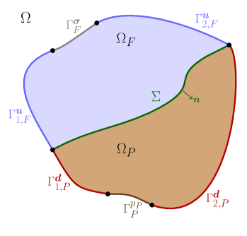
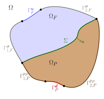
Figure 1.1: A configuration of subdomains and boundary partition for the Biot-Stokes coupled problem. (Left) Setup assumed for the analysis in Theorem 3.1. (Right) Example of another configuration investigated by some of the numerical experiments in Section 4.4.

For generic Sobolev spaces $X,Y$ and a scalar $\zeta>0$, the weighted space $\zeta X$ refers to $X$ endowed with the norm $\zeta\|\cdot\|_{X}$. The intersection $X\cap Y$ provided with the norm $\|v\|^{2}_{X\cap Y}=\|v\|^{2}_{X}+\|v\|_{Y}^{2}$, is a Hilbert space [30, 31].

Vector fields and vector-valued spaces will be written in boldface. In addition, by $L^{2}(\Omega)$ we will denote the usual Lebesgue space of square integrable functions and $H^{m}(\Omega)$ denotes the usual Sobolev space with weak derivatives of order up to $m$ in $L^{2}(\Omega)$, and $\mathbf{H}^{m}(\Omega)$ denotes its vector counterpart. In addition, $\mathbf{L}_{\boldsymbol{t}}^{2}(\Sigma)$ will denote the space of functions $\boldsymbol{z}:\Omega_{i}\to\mathbb{R}^{d}$, $i\in\{F,P\}$, such that $\boldsymbol{z}-\boldsymbol{n}(\boldsymbol{z}\cdot\boldsymbol{n})\in\mathbf{L}^{2}(\Sigma)$.

An $L^{2}(\Omega)$ (as well as $\mathbf{L}^{2}(\Omega)$) inner product over a generic bounded domain $\Omega$ is denoted as $(\cdot,\cdot)_{\Omega}$. The symbol $\langle\cdot,\cdot\rangle_{\Sigma}$ will denote the pairing between the trace functional space $H^{1/2}(\Sigma)$ and its dual $H^{-1/2}(\Sigma)$, and we will also write $\langle\cdot,\cdot\rangle$ to denote other, more general, duality pairings. Moreover, for $\boldsymbol{z}\in\mathbf{H}^{1}(\Omega_{i})\cap\mathbf{L}^{2}_{\boldsymbol{t}}(\Sigma)$, its normal and tangential traces defined by bounded surjective maps, will be denoted by $T_{\boldsymbol{n}}\boldsymbol{z}\in H^{1/2}(\Sigma)$ and $T_{\boldsymbol{t}}\boldsymbol{z}\in\mathbf{L}^{2}(\Sigma)$, respectively [23]. We also remark that, while $H^{1/2}(\Sigma)$ is a subspace of $L^{2}(\Sigma)$ as a set, the tangential trace of $\boldsymbol{z}\in\zeta_{1}\mathbf{H}^{1}(\Omega_{i})\cap\zeta_{2}\mathbf{L}^{2}_{\boldsymbol{t}}(\Sigma)$ is in $\zeta_{1}\mathbf{H}^{1/2}(\Sigma)\cap\zeta_{2}\mathbf{L}^{2}(\Sigma)$ and that in our setting it is important to track the parameter dependence for the sake of robustness.

Pertaining to the poroelastic domain, and assuming momentarily that $|\Gamma^{\boldsymbol{d}}_{P}|=0$, we recall from [32, Section 2.4.2] the definition of the space

$$H_{00}^{1/2}(\Sigma)=\{\eta\in H^{1/2}(\Sigma):\ E_{00}(\eta)\in H^{1/2}(\partial\Omega_{P})\},$$ (1.1)

supplied with the norm

$$\|\eta\|_{1/2,00,\Sigma}:=\|E_{00}(\eta)\|_{1/2,\partial\Omega_{P}},$$

where $E_{00}:H^{1/2}(\Sigma)\to H^{1/2}(\partial\Omega_{P})$ denotes the extension-by-zero operator

$$E_{00}(\eta)=\begin{cases}\eta&\text{on $\Sigma$},\\ 0&\text{on $\partial\Omega_{P}\setminus\Sigma$},\end{cases}\qquad\forall\eta\in H^{1/2}(\Sigma).$$

Furthermore, the restriction of $\psi\in H^{-1/2}(\partial\Omega_{P})$ to $\Sigma$, defined as

$$\langle\psi|_{\Sigma},\eta\rangle_{\Sigma}=\langle\psi,E_{00}(\eta)\rangle_{\partial\Omega_{P}}\quad\forall\eta\in H^{1/2}_{00}(\Sigma),$$

belongs to the dual $[H_{00}^{1/2}(\Sigma)]^{\prime}$ of $H_{00}^{1/2}(\Sigma)$. Its norm is

$$\|\psi|_{\Sigma}\|_{-1/2,00,\Sigma}:=\sup_{0\neq\eta\in H_{00}^{1/2}(\Sigma)}\frac{\langle\psi|_{\Sigma},\eta\rangle_{\Sigma}}{\|\eta\|_{1/2,00,\Sigma}}=\sup_{0\neq\eta\in H_{00}^{1/2}(\Sigma)}\frac{\langle\psi,E_{00}(\eta)\rangle_{\partial\Omega_{P}}}{\|E_{00}(\eta)\|_{1/2,\partial\Omega_{P}}}.$$ (1.2)

The boundary setup in Figure 1.1 is such that $|\Gamma^{\boldsymbol{d}}_{P}|\cdot|\Gamma^{p_{P}}_{P}|>0$, and therefore a modification of (1.1)-(1.2) is required. With that purpose, we note that any $\eta\in H^{1/2}(\Sigma)$ can be continuously extended to $\varphi$ in the space

$$H_{01}^{1/2}(\Sigma):=\{\eta\in H^{1/2}(\Sigma):E_{01}(\eta)\in H^{1/2}(\Gamma_{1})\},$$ (1.3)

where $\bar{\Gamma}_{1}:=\bar{\Sigma}\cup\bar{\Gamma}_{1,P}^{\boldsymbol{d}}\cup\bar{\Gamma}_{2,P}^{\boldsymbol{d}}$ (see Figure 1.1, left), and

$$E_{01}(\eta)=\begin{cases}\eta&\text{on $\Sigma$},\\ 0&\text{on $\Gamma_{P}^{\boldsymbol{d}}$},\end{cases}\qquad\forall\eta\in H^{1/2}(\Sigma).$$

This treatment can be interpreted as replacing $H_{00}^{1/2}(\Sigma)$ by the space of functions $\eta\in H^{1/2}(\Sigma)$ such that $\xi^{-1/2}\eta\in L^{2}(\Sigma)$, where $\xi$ is a sufficiently regular trace function, positive on $\Sigma$, and vanishing only on $\Gamma^{\boldsymbol{d}}_{P}$ (see, for example, [33]).

The norm of the resulting extension $\varphi\in H_{01}^{1/2}(\Sigma)$ is defined analogously as before,

$$\|\varphi\|_{1/2,01,\Sigma}:=\|E_{01}(\varphi)\|_{1/2,\Gamma_{1}},$$ (1.4)

and therefore the restriction of a distribution to the interface, $\psi|_{\Sigma}$, is in the dual space $[H_{01}^{1/2}(\Sigma)]^{\prime}$ and its norm is

$$\|\psi|_{\Sigma}\|_{-1/2,01,\Sigma}:=\sup_{0\neq\eta\in H_{01}^{1/2}(\Sigma)}\frac{\langle\psi|_{\Sigma},\eta\rangle_{\Sigma}}{\|\eta\|_{1/2,01,\Sigma}}=\sup_{0\neq\eta\in H_{01}^{1/2}(\Sigma)}\frac{\langle\psi,E_{01}(\eta)\rangle_{\Gamma_{1}}}{\|E_{01}(\eta)\|_{1/2,\Gamma_{1}}}.$$ (1.5)

2 Governing equations and weak formulation

The momentum and mass balance equations for the flow in the fluid cavity are given by Stokes equations written in terms of fluid velocity $\boldsymbol{u}$ and fluid pressure $p_{F}$, whereas the non-viscous filtration flow through the porous skeleton can be described by Darcy’s law in terms of pressure head $p_{P}$, and the porous matrix elastostatics are stated in terms of the solid displacement $\boldsymbol{d}$. The coupled Biot-Stokes equations arising after a backward Euler semi-discretization in time, with time step $\Delta t$, read

$$-\mathop{\mathbf{div}}\nolimits[2\mu_{f}\boldsymbol{\epsilon}(\boldsymbol{u})-p_{F}\mathbf{I}] =\rho_{f}\boldsymbol{g} \text{in $\Omega_{F}$},$$ (2.1a)

$$\mathop{\mathrm{div}}\nolimits\boldsymbol{u} =0 \text{in $\Omega_{F}$},$$ (2.1b)

$$-\mathop{\mathbf{div}}\nolimits[2\mu_{s}\boldsymbol{\epsilon}(\boldsymbol{d})-\varphi\mathbf{I}] =\rho_{s}\boldsymbol{f} \text{in $\Omega_{P}$},$$ (2.1c)

$$\varphi-\alpha p_{P}+\lambda\mathop{\mathrm{div}}\nolimits\boldsymbol{d} =0 \text{in $\Omega_{P}$},$$ (2.1d)

$$\bigl{(}C_{0}+\frac{\alpha^{2}}{\lambda}\bigr{)}\frac{1}{\Delta t}p_{P}-\frac{\alpha}{(\Delta t)\lambda}\varphi-\mathop{\mathrm{div}}\nolimits\biggl{(}\frac{\kappa}{\mu_{f}}\nabla p_{P}-\rho_{f}\boldsymbol{g}\biggr{)} =m_{P} \text{in $\Omega_{P}$},$$ (2.1e)

where $\boldsymbol{f}$ is a vector field of body loads, $\boldsymbol{g}$ is the gravity acceleration, $\mu_{f}$ is the fluid viscosity, $\boldsymbol{\epsilon}(\boldsymbol{u})=\frac{1}{2}(\nabla\boldsymbol{u}+\nabla\boldsymbol{u}^{\tt t})$ is the strain rate tensor, and $\boldsymbol{\epsilon}(\boldsymbol{d})=\frac{1}{2}(\nabla\boldsymbol{d}+\nabla\boldsymbol{d}^{\tt t})$ is the infinitesimal strain tensor, $\rho_{f},\rho_{s}$ are the density of the fluid and solid, respectively, $\lambda,\mu_{s}$ are the first and second Lamé constants of the solid, $\kappa$ is the heterogeneous tensor of permeabilities (satisfying $|\boldsymbol{w}|^{2}\lesssim\boldsymbol{w}\cdot\kappa(\boldsymbol{x})\boldsymbol{w}$ a.e. in $\Omega_{P}$ and for all $\boldsymbol{w}\in\mathbb{R}^{d}$); $m_{P}$ is a source/sink term for the fluid pressure (which also includes pressures in the previous backward Euler time step); and $C_{0},\alpha$ are the total storage capacity and Biot-Willis poroelastic coefficient. Here we have used the total pressure $\varphi:=\alpha p_{P}-\lambda\mathop{\mathrm{div}}\nolimits\boldsymbol{d}$, as an additional unknown [27, 20].

We furthermore supply boundary conditions as follows

$$\boldsymbol{u} =\boldsymbol{0} \text{on $\Gamma_{F}^{\boldsymbol{u}}$},$$ (2.2a)

$$[2\mu_{f}\boldsymbol{\epsilon}(\boldsymbol{u})-p_{F}\mathbf{I}]\boldsymbol{n} =\boldsymbol{0} \text{on $\Gamma_{F}^{\boldsymbol{\sigma}}$},$$ (2.2b)

$$\boldsymbol{d}=\boldsymbol{0}\quad\text{and}\quad\frac{\kappa}{\mu_{f}}\nabla p_{P}\cdot\boldsymbol{n} =0 \text{on $\Gamma_{P}^{\boldsymbol{d}}$},$$ (2.2c)

$$[2\mu_{s}\boldsymbol{\epsilon}(\boldsymbol{d})-\varphi\mathbf{I}]\boldsymbol{n}=\boldsymbol{0}\quad\text{and}\quad p_{P} =p_{0} \text{on $\Gamma_{P}^{p_{P}}$}.$$ (2.2d)

In order to close the system, we consider the classical transmission conditions on $\Sigma$ accounting for the continuity of normal fluxes, momentum balance, equilibrium of fluid normal stresses, and the so-called Beavers-Joseph-Saffman condition for tangential fluid forces [7, 2], which in the present setting reduce to

$$\boldsymbol{u}\cdot\boldsymbol{n} =(\frac{1}{\Delta t}\boldsymbol{d}-\frac{\kappa}{\mu_{f}}\nabla p_{P})\cdot\boldsymbol{n} \text{on $\Sigma$},$$ (2.3a)

$$(2\mu_{f}\boldsymbol{\epsilon}(\boldsymbol{u})-p_{F}\mathbf{I})\boldsymbol{n} =(2\mu_{s}\boldsymbol{\epsilon}(\boldsymbol{d})-\varphi\mathbf{I})\boldsymbol{n} \text{on $\Sigma$},$$ (2.3b)

$$-\boldsymbol{n}\cdot(2\mu_{f}\boldsymbol{\epsilon}(\boldsymbol{u})-p_{F}\mathbf{I})\boldsymbol{n} =p_{P} \text{on $\Sigma$},$$ (2.3c)

$$-\boldsymbol{n}\cdot(2\mu_{f}\boldsymbol{\epsilon}(\boldsymbol{u})-p_{F}\mathbf{I})\boldsymbol{t}_{j} =\frac{\gamma\mu_{f}}{\sqrt{\kappa}}(\boldsymbol{u}-\frac{1}{\Delta t}\boldsymbol{d})\cdot\boldsymbol{t}_{j},\quad 1\leq j\leq d-1 \text{on $\Sigma$},$$ (2.3d)

where $\gamma>0$ is the slip rate coefficient depending on the geometry of the domain, and we recall that the normal $\boldsymbol{n}$ on the interface is understood as pointing from the fluid domain $\Omega_{F}$ towards the porous structure $\Omega_{P}$, while $\boldsymbol{t}_{j}$, $1\leq j\leq d-1$ are orthonormal tangent vectors on $\Sigma$, normal to $\boldsymbol{n}$.

We proceed to test (2.1a)-(2.1e) against suitable smooth functions and to integrate over the corresponding subdomain. The challenging model parameters are $\mu_{f}$, $C_{0}$, $\lambda$, $\gamma$, $\alpha$, and the magnitude of $\kappa$. Therefore, we will concentrate on the specific case where $\Delta t=1$, and the model parameters (in particular $\kappa$) are spatially constant. Following [24], after applying integration by parts wherever adequate and using the transmission conditions (2.3a)-(2.3d), we arrive at the following remainder on the interface

$$\langle p_{P},(\boldsymbol{v}-\boldsymbol{w})\cdot\boldsymbol{n}\rangle_{\Sigma}+\frac{\gamma\mu_{f}}{\sqrt{\kappa}}\sum_{j=1}^{d-1}\langle(\boldsymbol{u}-\boldsymbol{d})\cdot\boldsymbol{t}_{j},(\boldsymbol{v}-\boldsymbol{w})\cdot\boldsymbol{t}_{j}\rangle_{\Sigma}+\langle(\boldsymbol{u}-\boldsymbol{d})\cdot\boldsymbol{n},q_{P}\rangle_{\Sigma},$$

which is well-defined and therefore no additional Lagrange multipliers are required to realize the coupling conditions. Also, in view of the character of the resulting variational forms in combination with the specification of boundary conditions (2.2), we define the Hilbert spaces

$$\mathbf{H}^{1}_{\star}(\Omega_{F})=\{\boldsymbol{v}\in\mathbf{H}^{1}(\Omega_{F}):\boldsymbol{v}|_{\Gamma_{F}^{\boldsymbol{u}}}=\boldsymbol{0}\},\quad\mathbf{H}^{1}_{\star}(\Omega_{P})=\{\boldsymbol{w}\in\mathbf{H}^{1}(\Omega_{P}):\boldsymbol{w}|_{\Gamma_{P}^{\boldsymbol{d}}}=\boldsymbol{0}\},$$

$$H^{1}_{\star}(\Omega_{P})=\{q_{P}\in H^{1}(\Omega_{P}):q_{P}|_{\Gamma_{P}^{p_{P}}}=0\},$$

and the product space $\mathbf{H}$

$$\mathbf{H}=\mathbf{H}^{1}_{\star}(\Omega_{F})\times\mathbf{H}^{1}_{\star}(\Omega_{P})\times L^{2}(\Omega_{F})\times L^{2}(\Omega_{P})\times H^{1}_{\star}(\Omega_{P}).$$ (2.4)

Consequently, we have the following weak form for the Biot-Stokes coupling: Find $(\boldsymbol{u},\boldsymbol{d},p_{F},\varphi,p_{P})\in\mathbf{W}$ such that

$$2\mu_{f}(\boldsymbol{\epsilon}(\boldsymbol{u}),\boldsymbol{\epsilon}(\boldsymbol{v}))_{\Omega_{F}}+\frac{\gamma\mu_{f}}{\sqrt{\kappa}}\langle T_{\boldsymbol{t}}(\boldsymbol{u}-\boldsymbol{d}),T_{\boldsymbol{t}}\boldsymbol{v}\rangle_{\Sigma}$$

$$-(p_{F},\mathop{\mathrm{div}}\nolimits\boldsymbol{v})_{\Omega_{F}}+\langle p_{P},T_{\boldsymbol{n}}\boldsymbol{v}\rangle_{\Sigma} =F^{F}(\boldsymbol{v}) \forall\boldsymbol{v}\in\mathbf{H}^{1}_{\star}(\Omega_{F}),$$ (2.5a)

$$\frac{\gamma\mu_{f}}{\sqrt{\kappa}}\langle T_{\boldsymbol{t}}(\boldsymbol{d}-\boldsymbol{u}),T_{\boldsymbol{t}}\boldsymbol{w}\rangle_{\Sigma}+2\mu_{s}(\boldsymbol{\epsilon}(\boldsymbol{d}),\boldsymbol{\epsilon}(\boldsymbol{w}))_{\Omega_{P}}$$

$$-(\varphi,\mathop{\mathrm{div}}\nolimits\boldsymbol{w})_{\Omega_{P}}-\langle p_{P},T_{\boldsymbol{n}}\boldsymbol{w}\rangle_{\Sigma} =F^{P}(\boldsymbol{w}) \forall\boldsymbol{w}\in\mathbf{H}^{1}_{\star}(\Omega_{P}),$$ (2.5b)

$$-(\mathop{\mathrm{div}}\nolimits\boldsymbol{u},q_{F})_{\Omega_{F}} =0 \forall q_{F}\in L^{2}(\Omega_{F}),$$ (2.5c)

$$\frac{1}{\lambda}(\alpha p_{P}-\varphi,\psi)_{\Omega_{P}}-(\mathop{\mathrm{div}}\nolimits\boldsymbol{d},\psi)_{\Omega_{P}} =0 \forall\psi\in L^{2}(\Omega_{P}),$$ (2.5d)

$$-\bigl{(}C_{0}+\frac{\alpha^{2}}{\lambda}\bigr{)}(p_{P},q_{P})_{\Omega_{P}}+\frac{\alpha}{\lambda}(q_{P},\varphi)_{\Omega_{P}}\qquad\quad$$

$$+\langle q_{P},T_{\boldsymbol{n}}(\boldsymbol{u}-\boldsymbol{d})\rangle_{\Sigma}-\frac{\kappa}{\mu_{f}}(\nabla q_{P},\nabla p_{P})_{\Omega_{P}} =G(q_{P}) \forall q_{P}\in H^{1}_{\star}(\Omega_{P}),$$ (2.5e)

where

$$F^{F}(\boldsymbol{v})=\rho_{f}(\boldsymbol{g},\boldsymbol{v})_{\Omega_{F}},\quad F^{P}(\boldsymbol{w})=\rho_{s}(\boldsymbol{f},\boldsymbol{w})_{\Omega_{P}},\quad G(q_{P})=-(m_{P},q_{P})_{\Omega_{P}}-\rho_{f}(\boldsymbol{g},\nabla q_{P})_{\Omega_{P}}+\rho_{f}\langle\boldsymbol{g}\cdot\boldsymbol{n},q_{P}\rangle_{\Sigma}.$$

System (2.5) differs from that analyzed in [16] in the ordering of the unknowns, and in that we obtain a symmetric multilinear formulation defined by a global operator $\mathcal{A}$ (the coefficient matrix of the left-hand side of (2.5)) of the form

$$\small{\left(\begin{array}[]{cc:ccc}-2\mu_{f}\mathop{\mathbf{div}}\nolimits\boldsymbol{\epsilon}+\frac{\gamma\mu_{f}}{\sqrt{\kappa}}T_{\boldsymbol{t}}^{\prime}T_{\boldsymbol{t}}&-\frac{\gamma\mu_{f}}{\sqrt{\kappa}}T_{\boldsymbol{t}}^{\prime}&\nabla&&T_{\boldsymbol{n}}^{\prime}\\ -\frac{\gamma\mu_{f}}{\sqrt{\kappa}}T_{\boldsymbol{t}}&\!\!\!\!\!-2\mu_{s}\mathop{\mathbf{div}}\nolimits\boldsymbol{\epsilon}+\frac{\gamma\mu_{f}}{\sqrt{\kappa}}T_{\boldsymbol{t}}^{\prime}T_{\boldsymbol{t}}&&\!\!\!\!\!\!\!\nabla&-T_{\boldsymbol{n}}^{\prime}\vphantom{\int^{X^{X}}}\\[3.87498pt] \hdashline-\mathop{\mathrm{div}}\nolimits&&&&\\ &-\mathop{\mathrm{div}}\nolimits&&\!\!\!\!\!\!\!-\frac{1}{\lambda}I&\frac{\alpha}{\lambda}I\\[3.87498pt] T_{\boldsymbol{n}}&-T_{\boldsymbol{n}}&&\!\!\!\!\!\!\!\frac{\alpha}{\lambda}I&\!\!\!\!\!-\bigl{(}C_{0}+\frac{\alpha^{2}}{\lambda}\bigr{)}I+\frac{\kappa}{\mu_{f}}\Delta\end{array}\right),}$$ (2.6)

where the dependence on the model parameters is clearly identified. In particular, the interface coupling terms on the first off-diagonal blocks depend on the inverse of permeability.

We note that $\mathcal{A}$ can be regarded as defining a perturbed saddle-point problem, with

$$\mathcal{A}=\begin{pmatrix}A&B^{\prime}\\ B&-C\\ \end{pmatrix},$$

where the composing blocks are defined as

$$A=\begin{pmatrix}\mathcal{A}_{FF}&\mathcal{A}_{FP}\\ \mathcal{A}_{PF}&\mathcal{A}_{PP}\end{pmatrix}=\begin{pmatrix}-2\mu_{f}\mathop{\mathbf{div}}\nolimits\boldsymbol{\epsilon}&0\\ 0&-2\mu_{s}\mathop{\mathbf{div}}\nolimits\boldsymbol{\epsilon}\\ \end{pmatrix}+\gamma\frac{\mu_{f}}{\sqrt{\kappa}}\begin{pmatrix}T_{\boldsymbol{t}}^{\prime}\\ -T_{\boldsymbol{t}}^{\prime}\end{pmatrix}\begin{pmatrix}T_{\boldsymbol{t}}&-T_{\boldsymbol{t}}\end{pmatrix},$$ (2.7a)

$$B=\begin{pmatrix}-\mathop{\mathrm{div}}\nolimits&0\\ 0&-\mathop{\mathrm{div}}\nolimits\\ T_{\boldsymbol{n}}&-T_{\boldsymbol{n}}\\ \end{pmatrix},\quad C=\begin{pmatrix}0&0&0\\ 0&\frac{1}{\lambda}I&-\frac{\alpha}{\lambda}I\\ 0&-\frac{\alpha}{\lambda}I&\bigl{(}C_{0}+\frac{\alpha^{2}}{\lambda}\bigr{)}I-\frac{\kappa}{\mu_{f}}\Delta\end{pmatrix}.$$ (2.7b)

In turn, well-posedness of the Biot-Stokes system (2.5) in the product space (2.4) can be established using the abstract Brezzi-Braess theory [34], after invoking separately the solvability and stability results for the Stokes subproblem [35] and the Biot subproblem in the three-field total pressure formulation [27]. However, such a decoupled approach does not lead to stability independent of the material parameters and consequently, preconditioners based on the standard norms (also referred to as single-physics or sub-physics preconditioners) are not necessarily parameter robust. This issue is demonstrated next in Example 2.1.

Example 2.1 (Simple preconditioners using standard norms).

We consider the Biot-Stokes formulation (2.5) defined on the subdomains $\Omega_{F}=(0,\tfrac{1}{2})\times(0,1)$, $\Omega_{P}=(\tfrac{1}{2},1)\times(0,1)$ with boundary conditions such that the left edge of $\Omega_{F}$ is a no-slip boundary $\Gamma_{F}^{\boldsymbol{u}}$ while the top and bottom edges will form $\Gamma^{\boldsymbol{\sigma}}_{F}$. Similarly, the top and bottom edges on the Biot side are considered stress-free while the right edge is clamped.

Based on the well-posedness of (2.5) in the space $\mathbf{H}$ (cf. (2.4)), we can readily consider a solution space with weighted inner product leading to the Riesz map (diagonal) preconditioner

$$\mathcal{R}_{D}=\begin{pmatrix}\mathcal{A}_{FF}&&&&\\ &\!\!\!\!\!\mathcal{A}_{PP}&&&\\ &&\!\!\!\!\!\frac{1}{2\mu_{f}}I&&\\ &&&\!\!\!\!\!\bigl{(}\frac{1}{\lambda}+\frac{1}{2\mu_{s}}\bigr{)}I&\\ &&&&\!\!\!\!\!\!\bigl{(}C_{0}+\frac{\alpha^{2}}{\lambda}\bigr{)}I-\frac{\kappa}{\mu_{f}}\Delta\end{pmatrix}^{-1}.$$ (2.8)

We remark that the first and third blocks of $\mathcal{R}_{D}$ together define a parameter robust preconditioner for the (standalone) Stokes problem and the remaining blocks form the robust three-field Biot preconditioner [27]. However, in $\mathcal{R}_{D}$ the subproblem preconditioners are decoupled.

Alternatively, after observing that the operator $A$ in (2.7a) defines a norm over the velocity-displacement space $\mathbf{H}^{1}_{\star}(\Omega_{F})\times\mathbf{H}^{1}_{\star}(\Omega_{P})$ we will also investigate the (block-diagonal) preconditioner

$$\mathcal{R}_{C}=\begin{pmatrix}\mathcal{A}_{FF}&\mathcal{A}_{FP}&&&\\ \mathcal{A}_{PF}&\!\!\!\!\mathcal{A}_{PP}&&&\\ &&\!\!\!\!\!\frac{1}{2\mu_{f}}I&&\\ &&&\!\!\!\!\!\bigl{(}\frac{1}{\lambda}+\frac{1}{2\mu_{s}}\bigr{)}I&\\ &&&&\!\!\!\!\!\!\bigl{(}C_{0}+\frac{\alpha^{2}}{\lambda}\bigr{)}I-\frac{\kappa}{\mu_{f}}\Delta\end{pmatrix}^{-1}.$$ (2.9)

We note that in (2.9) the tangential components of the Stokes velocity and of the Biot displacement are coupled. In this sense, the preconditioner captures the interaction between the subsystems and, in particular, the coupling through the Beavers-Joseph-Saffman condition (2.3d).

To investigate the robustness of these preconditioners, we set typical physical parameters in (2.5) except for $\mu_{f}$ and $\kappa$, which are to be varied. Using a discretization in terms of the lowest-order Taylor-Hood elements (see more details in Section 4.1), we next consider the boundedness of the number of iterations of the preconditioned MinRes solver under mesh refinement and parameter variations. More precisely, using $\mathcal{R}_{D}$, $\mathcal{R}_{C}$ (inverted by LU) we compare the number of iterations required for convergence determined by reducing the preconditioned residual norm by a factor $10^{8}$. The initial vector is taken as random.

We report the results in Table 2.1. It can be seen that the number of MinRes iterations produced with the diagonal preconditioner $\mathcal{R}_{D}$ is rather sensitive to variations in both $\mu_{f}$ and $\kappa$. In comparison, when fixing $\mu_{f}=1$, the iterations appear to be more stable in $\kappa$ when (2.9) is used. However, if $\kappa=1$ is set, there is a clear deterioration of the performance for small values of $\mu_{f}$ also with the preconditioner $\mathcal{R}_{C}$.

		Preconditioner (2.8)				Preconditioner (2.9)
$\mu_{f}$		$2^{-2}$	$2^{-3}$	$2^{-4}$	$2^{-5}$	$2^{-2}$	$2^{-3}$	$2^{-4}$	$2^{-5}$
$1$	$10^{-4}$	211	240	258	264	71	82	89	89
	$10^{-2}$	76	76	74	73	50	49	48	48
	$1$	41	41	41	41	37	37	36	36
$\kappa$		$2^{-2}$	$2^{-3}$	$2^{-4}$	$2^{-5}$	$2^{-2}$	$2^{-3}$	$2^{-4}$	$2^{-5}$
$1$	$10^{-8}$	394	184	–	–	693	471	639	–
	$10^{-2}$	59	59	59	58	58	57	55	55
	$1$	41	41	41	41	37	37	36	36

Table 2.1: Performance of preconditioners (2.8) and (2.9) for the Biot-Stokes system (2.5) in Example 2.1. Only the parameters $\mu_{f}$ and $\kappa$ are varied away from 1. The lack of convergence after 750 MinRes iterations is indicated as –.

The improved performance of the preconditioner $\mathcal{R}_{C}$, which preserves the tangential coupling of the Stokes and Biot problems in (2.3d), over $\mathcal{R}_{D}$, where the components are decoupled, suggests to strengthening the coupling (involving the tangential traces) in order to obtain parameter robustness. However, from the point of view of the interface conditions (2.3a)-(2.3d), it is clear that the coupling in the normal direction is missing in $\mathcal{R}_{C}$.

With the above idea in mind, we proceed to establish well-posedness of (2.5) in the product space equipped with non-standard norms that include additional control at the interface reflecting/arising from the mass conservation condition (2.3a).

3 Well-posedness of the Biot-Stokes system

Let us group the variables as $\vec{\boldsymbol{u}}=(\boldsymbol{u},\boldsymbol{d})$ and $\vec{p}=(p_{F},\varphi,p_{P})$ and introduce the weighted norm

$$\|(\vec{\boldsymbol{u}},\vec{p})\|_{\mathbf{H}_{\epsilon}}^{2}:=\|\vec{\boldsymbol{u}}\|_{A}^{2}+|\vec{p}|_{B}^{2}+|\vec{p}|_{C}^{2},$$ (3.1)

with

$$\|\vec{\boldsymbol{u}}\|_{A}^{2} :=2\mu_{f}\|\boldsymbol{\epsilon}(\boldsymbol{u})\|^{2}_{0,\Omega_{F}}+\sum_{j=1}^{d-1}\frac{\gamma\mu_{f}}{\sqrt{\kappa}}\|(\boldsymbol{u}-\boldsymbol{d})\cdot\boldsymbol{t}_{j}\|^{2}_{0,\Sigma}+2\mu_{s}\|\boldsymbol{\epsilon}(\boldsymbol{d})\|^{2}_{0,\Omega_{P}},$$ (3.2a)

$$|\vec{p}|_{B}^{2} :=\frac{1}{{2\mu_{f}}}\|p_{F}\|^{2}_{0,\Omega_{F}}+\frac{1}{2\mu_{s}}\|\varphi\|^{2}_{0,\Omega_{P}}+\left(\frac{1}{2\mu_{f}}+\frac{1}{2\mu_{s}}\right){\|p_{P}|_{\Sigma}\|^{2}_{-\frac{1}{2},01,\Sigma}},$$ (3.2b)

$$|\vec{p}|_{C}^{2} :=\frac{1}{\lambda}\|\varphi-\alpha p_{P}\|^{2}_{0,\Omega_{P}}+C_{0}\|p_{P}\|^{2}_{0,\Omega_{P}}+\frac{\kappa}{\mu_{f}}\|\nabla p_{P}\|^{2}_{0,\Omega_{P}},$$ (3.2c)

where the fractional norm is defined in (1.5).

In turn, we define the weighted product space $\mathbf{H}_{\epsilon}$ as the space that contains all $(\vec{\boldsymbol{u}},\vec{p})$ that are bounded in this norm. The subscript $\epsilon$ encodes the collection of weighting parameters $\kappa,\alpha,\gamma,\mu_{f},\mu_{s},C_{0},\lambda$. Moreover, the space allows for the natural decomposition:

$$\mathbf{H}_{\epsilon}=\vec{\mathbf{V}}\times\vec{Q}.$$

Theorem 3.1.

Problem (2.5) is well-posed in the space $\mathbf{H}_{\epsilon}$ equipped with the norm (3.1). In other words, the operator $\mathcal{A}:\mathbf{H}_{\epsilon}\to\mathbf{H}_{\epsilon}^{\prime}$ in (2.6) is a symmetric isomorphism satisfying

$$\|\mathcal{A}\|_{\mathcal{L}(\mathbf{H}_{\epsilon},\mathbf{H}_{\epsilon}^{\prime})}\leq C_{1},$$ (3.3a)

$$\|\mathcal{A}^{-1}\|_{\mathcal{L}(\mathbf{H}_{\epsilon}^{\prime},\mathbf{H}_{\epsilon})}\leq C_{2},$$ (3.3b)

where $C_{1},C_{2}$ are positive constants independent of $\epsilon$.

Proof.

The operator norm is defined as

$$\|\mathcal{A}\|_{\mathcal{L}(\mathbf{H}_{\boldsymbol{\epsilon}},\mathbf{H}_{\boldsymbol{\epsilon}}^{\prime})}:=\sup_{(\vec{\boldsymbol{u}},\vec{p}),(\vec{\boldsymbol{v}},\vec{q})}\frac{\langle\mathcal{A}(\vec{\boldsymbol{u}},\vec{p}),(\vec{\boldsymbol{v}},\vec{q})\rangle}{\|(\vec{\boldsymbol{u}},\vec{p})\|_{\mathbf{H}_{\boldsymbol{\epsilon}}}||(\vec{\boldsymbol{v}},\vec{q})||_{\mathbf{H}_{\boldsymbol{\epsilon}}^{\prime}}},$$

and condition (3.3a) states the continuity of $\mathcal{A}$. To show this, we first use the Cauchy-Schwarz inequality to derive

$$\langle A\vec{\boldsymbol{u}},\vec{\boldsymbol{v}}\rangle \leq\|\vec{\boldsymbol{u}}\|_{A}\|\vec{\boldsymbol{v}}\|_{A}, \langle C\vec{p},\vec{q}\rangle \leq|\vec{p}|_{C}|\vec{q}|_{C}.$$ (3.4)

It therefore remains to show that $B$ is continuous. Another application of the Cauchy-Schwarz inequality on the different terms together with a trace inequality provides this result.

In order to prove the second relation (3.3b), we aim to verify the assumptions of the Banach-Nečas-Babuška (BNB) theorem (see, e.g., [36]). In particular, we aim to prove that

$$\sup_{(\vec{\boldsymbol{v}},\vec{p})}\frac{\langle\mathcal{A}(\vec{\boldsymbol{u}},\vec{p}),(\vec{\boldsymbol{v}},\vec{q})\rangle}{\|(\vec{\boldsymbol{v}},\vec{q})\|_{\mathbf{H}_{\epsilon}}} \gtrsim\|(\vec{\boldsymbol{u}},\vec{p})\|_{\mathbf{H}_{\epsilon}}, \forall(\vec{\boldsymbol{u}},\vec{p}) \in\mathbf{H}_{\epsilon}.$$ (3.5)

We do this by assuming that $(\vec{\boldsymbol{u}},\vec{p})\in\mathbf{H}_{\epsilon}$ is given and by constructing an appropriate test function $(\vec{\boldsymbol{v}},\vec{q})\in\mathbf{H}_{\epsilon}$. Following, e.g., [37, 27], we choose $\vec{q}=-\vec{p}$ and $\vec{\boldsymbol{v}}=\vec{\boldsymbol{u}}$, giving

$$\langle\mathcal{A}(\vec{\boldsymbol{u}},\vec{p}),(\vec{\boldsymbol{u}},-\vec{p})\rangle =\langle A\vec{\boldsymbol{u}},\vec{\boldsymbol{u}}\rangle+\langle B\vec{\boldsymbol{u}},\vec{p}\rangle-\langle B\vec{\boldsymbol{u}},\vec{p}\rangle+\langle C\vec{p},\vec{p}\rangle$$

$$=\|\vec{\boldsymbol{u}}\|_{A}^{2}+|\vec{p}|_{C}^{2}.$$ (3.6)

Next, the inf-sup condition proven in Lemma 3.1, below, allows us to construct $\vec{\boldsymbol{v}}_{p}$ such that

$$\langle B\vec{\boldsymbol{v}}_{p},\vec{p}\,\rangle =|\vec{p}|_{B}^{2}, \|\vec{\boldsymbol{v}}_{p}\|_{A} \leq\beta_{0}^{-1}|\vec{p}|_{B}.$$ (3.7)

We now use this test function, scaled by a constant $\delta>0$ to be chosen later, and using (3.2a)-(3.2c) along with (3.4) and (3.7), we derive

$$\langle\mathcal{A}(\vec{\boldsymbol{u}},\vec{p}),(\delta\vec{\boldsymbol{v}}_{p},\vec{0})\rangle =\langle A\vec{\boldsymbol{u}},\delta\vec{\boldsymbol{v}}_{p}\rangle+\delta[B\vec{\boldsymbol{v}}_{p},\vec{p}]$$

$$\geq-\delta\|\vec{\boldsymbol{u}}\|_{A}\|\vec{\boldsymbol{v}}_{p}\|_{A}+\delta|\vec{p}|_{B}^{2}$$

$$\geq-\frac{1}{2}\|\vec{\boldsymbol{u}}\|_{A}^{2}-\frac{1}{2}\delta^{2}\|\vec{\boldsymbol{v}}_{p}\|_{A}^{2}+\delta|\vec{p}|_{B}^{2}$$

$$\geq-\frac{1}{2}\|\vec{\boldsymbol{u}}\|_{A}^{2}+(\delta-\frac{1}{2}\beta_{0}^{-2}\delta^{2})|\vec{p}|_{B}^{2},$$

where we have also used Cauchy-Schwarz and Young’s inequality. Setting $\delta=\beta_{0}^{2}$ gives us

$$\langle\mathcal{A}(\vec{\boldsymbol{u}},\vec{p}),(\delta\vec{\boldsymbol{v}}_{p},\vec{0})\rangle \geq-\frac{1}{2}\|\vec{\boldsymbol{u}}\|_{A}^{2}+\frac{1}{2}\beta_{0}^{2}|\vec{p}|_{B}^{2}.$$ (3.8)

Finally, we take $(\vec{\boldsymbol{v}},\vec{q})=(\vec{\boldsymbol{u}}+\delta\vec{\boldsymbol{v}}_{p},-\vec{p})$ and put together (3) and (3.8) to arrive at

$$\langle\mathcal{A}(\vec{\boldsymbol{u}},\vec{p}),(\vec{\boldsymbol{v}},\vec{q})\rangle \geq\frac{1}{2}\|\vec{\boldsymbol{u}}\|_{A}^{2}+\frac{1}{2}\beta_{0}^{2}|\vec{p}|_{B}^{2}+|\vec{p}|_{C}^{2}$$

$$\gtrsim\|(\vec{\boldsymbol{u}},\vec{p})\|_{\mathbf{H}_{\epsilon}}^{2},$$

$$\|(\vec{\boldsymbol{v}},\vec{q})\|_{\mathbf{H}_{\epsilon}}^{2} \leq 2\left(\|(\vec{\boldsymbol{u}},\vec{p})\|_{\mathbf{H}_{\epsilon}}^{2}+\delta^{2}\|\vec{\boldsymbol{v}}_{p}\|_{A}^{2}\right)$$

$$\leq 2\left(\|(\vec{\boldsymbol{u}},\vec{p})\|_{\mathbf{H}_{\epsilon}}^{2}+\beta_{0}^{2}|\vec{p}|_{B}^{2}\right)$$

$$\lesssim\|(\vec{\boldsymbol{u}},\vec{p})\|_{\mathbf{H}_{\epsilon}}^{2}.$$

The combination of these two bounds shows that (3.5) holds. The BNB theorem now provides (3.3b). ∎

Lemma 3.1.

There exists a $\beta_{0}>0$ such that

$$\sup_{\boldsymbol{0}\neq\vec{\boldsymbol{v}}}\frac{\langle B\vec{\boldsymbol{v}},\vec{p}\rangle}{\|\vec{\boldsymbol{v}}\|_{A}}\geq\beta_{0}|\vec{p}|_{B}\qquad\forall\vec{p}\in\vec{Q}.$$

Proof.

The proof follows similarly to [21, Section 3]. Let $\vec{p}=(p_{F},\varphi,p_{P})\in\vec{Q}$ be given. We proceed in five steps.

1. With a given total pressure $\varphi$ in the Biot domain, we set up an auxiliary Stokes problem: Find $(\boldsymbol{z}_{0},s_{0})\in\mathbf{H}^{1}(\Omega_{P})\times L^{2}(\Omega_{P})$ that weakly satisfy

   $$-\mathop{\mathbf{div}}\nolimits\left(\boldsymbol{\epsilon}(\boldsymbol{z}_{0})+s_{0}\mathbf{I}\right) =\boldsymbol{0},$$

   $$\mathop{\mathrm{div}}\nolimits\boldsymbol{z}_{0} =-\varphi \Omega_{P},$$ in

   subject to the mixed boundary conditions

   $$\boldsymbol{z}_{0} =\boldsymbol{0}\ \text{on}\quad\Gamma_{P}^{\boldsymbol{d}}\cup\Sigma, \text{and}\quad\left(\boldsymbol{\epsilon}(\boldsymbol{z}_{0})+s_{0}\mathbf{I}\right)\boldsymbol{n} =\boldsymbol{0}\ \text{on}\ \Gamma_{P}^{p_{P}}.$$

   By the well-posedness of this auxiliary problem (for a proof see, e.g., [35, Chapter I]), the first component of the solution satisfies

   $$\|\boldsymbol{z}_{0}\|_{1,\Omega_{P}}\lesssim\|\varphi\|_{0,\Omega_{P}}.$$

2. We next consider that the trace of $p_{P}$ is a distribution in $H^{-1/2}(\partial\Omega_{P})$, and focus on its restriction to the interface, $p_{P}|_{\Sigma}$, belonging to $[H_{01}^{1/2}(\Sigma)]^{\prime}$ (cf., the end of Section 1).

   Let $\zeta\in H_{01}^{1/2}(\Sigma)$ be the Riesz representative of $p_{P}|_{\Sigma}\in[H_{01}^{1/2}(\Sigma)]^{\prime}$, and consider a Stokes-extension of $\zeta$ into $\Omega_{P}$ by setting up another auxiliary Stokes problem (and still in the Biot domain): Find a pair $(\boldsymbol{z}_{1},s_{1})\in\mathbf{H}^{1}(\Omega_{P})\times L^{2}(\Omega_{P})$ that weakly satisfies

   $$-\mathop{\mathbf{div}}\nolimits\left(\boldsymbol{\epsilon}(\boldsymbol{z}_{1})+s_{1}\mathbf{I}\right) =\boldsymbol{0},$$ (3.10a)

   $$\mathop{\mathrm{div}}\nolimits\boldsymbol{z}_{1} =0 \Omega_{P},$$ in

   subject to the mixed-type boundary conditions

   $$\boldsymbol{z}_{1} =\zeta\boldsymbol{n}\ \text{on}\ \Sigma,$$ (3.10b)

   $$\boldsymbol{z}_{1} =\boldsymbol{0}\ \text{on}\ \Gamma_{P}^{\boldsymbol{d}}, \left(\boldsymbol{\epsilon}(\boldsymbol{z}_{1})+s_{1}\mathbf{I}\right)\boldsymbol{n} =\boldsymbol{0}\ \text{on}\ \Gamma_{P}^{p_{P}}.$$

   Again, we use the well-posedness of the auxiliary problem (in this case, (3.10)) to conclude that the extension function $\boldsymbol{z}_{1}$ satisfies a continuous dependence on data

   $$\|\boldsymbol{z}_{1}\|_{1,\Omega_{P}}\lesssim\|\zeta\|_{\frac{1}{2},01,\Sigma}=\|p_{P}\|_{-\frac{1}{2},01,\Sigma}.$$

3. We combine the two previous steps to form a Biot velocity as $\boldsymbol{v}_{P}:=\frac{1}{2\mu_{s}}(\boldsymbol{z}_{0}+\boldsymbol{z}_{1})$. By construction, this function has the following properties

   $$\langle B(\boldsymbol{v}_{P},\boldsymbol{0}),\vec{p}\rangle =-(\mathop{\mathrm{div}}\nolimits\boldsymbol{v}_{P},\varphi)_{\Omega_{P}}+\langle\boldsymbol{n}\cdot\boldsymbol{v}_{P},p_{P}\rangle_{\Sigma}$$

   $$=\frac{1}{2\mu_{s}}\left(-(\mathop{\mathrm{div}}\nolimits\boldsymbol{z}_{0},\varphi)_{\Omega_{P}}+\langle\boldsymbol{n}\cdot\boldsymbol{z}_{1},p_{P}\rangle_{\Sigma}\right)$$

   $$=\frac{1}{2\mu_{s}}\left(\|\varphi\|_{\Omega_{P}}^{2}+\|p_{P}|_{\Sigma}\|_{-\frac{1}{2},01,\Sigma}^{2}\right),$$

   $$\|(\boldsymbol{v}_{P},\boldsymbol{0})\|_{A}^{2} =2\mu_{s}\|\boldsymbol{\epsilon}(\boldsymbol{v}_{P})\|^{2}_{0,\Omega_{P}}$$

   $$\leq\frac{1}{2\mu_{s}}2\left(\|\boldsymbol{z}_{0}\|^{2}_{1,\Omega_{P}}+\|\boldsymbol{z}_{1}\|^{2}_{1,\Omega_{P}}\right)$$

   $$\lesssim\frac{1}{2\mu_{s}}\left(\|\varphi\|_{\Omega_{P}}^{2}+\|p_{P}|_{\Sigma}\|_{-\frac{1}{2},01,\Sigma}^{2}\right).$$

4. Next, we repeat the first three steps with $p_{F}$ substituted for $\varphi$, $-\zeta$ for $\zeta$, $\Omega_{F}$ instead of $\Omega_{P}$ (as well as the relevant boundaries), and $\mu_{f}$ substituted for $\mu_{s}$. In particular, for step 2 we note that the Riesz representative $\zeta$ is constructed relatively to $\partial\Omega_{P}$, but the trace of $\mathbf{H}_{\star}^{1}(\Omega_{F})$ can be regarded as equivalent to the trace of $\mathbf{H}_{\star}^{1}(\Omega_{P})$ provided that the shapes and measures of each subdomains are similar (see [38, 39], where the argument is applied to a normal velocity trace on the interface). Then one can also consider $\zeta\in H_{01}^{1/2}(\Sigma)$, as relative to $\partial\Omega_{F}$.

   In this case we end up with a Stokes velocity $\boldsymbol{v}_{F}$ satisfying the relations

   $$\langle B(\boldsymbol{v}_{F},\boldsymbol{0}),\vec{p}\rangle =\frac{1}{2\mu_{f}}\left(\|p_{F}\|_{\Omega_{F}}^{2}+\|p_{P}|_{\Sigma}\|_{-\frac{1}{2},01,\Sigma}^{2}\right),$$

   $$\|(\boldsymbol{v}_{F},\boldsymbol{0})\|_{A}^{2} \lesssim\frac{1}{2\mu_{f}}\left(\|p_{F}\|_{\Omega_{F}}^{2}+\|p_{P}|_{\Sigma}\|_{-\frac{1}{2},01,\Sigma}^{2}\right).$$

5. For the final step it suffices to combine steps 3 and 4, and choose as test function the pair of functions constructed above $\vec{\boldsymbol{v}}=(\boldsymbol{v}_{F},\boldsymbol{v}_{P})$, which leads to

   $$\langle B\vec{\boldsymbol{v}},\vec{p}\,\rangle =|\vec{p}|_{B}^{2}, \|\vec{\boldsymbol{v}}\|_{A}^{2} \lesssim|\vec{p}|_{B}^{2}.$$ (3.11)

Equation (3.11) also contains the right scaling through the use of the $|\cdot|_{B}$ seminorm. This step concludes the proof. ∎

According to the general operator preconditioning framework from [25], Theorem 3.1 yields that a parameter-robust preconditioner can be constructed based on the Riesz map $\mathcal{R}:\mathbf{H}_{\epsilon}^{\prime}\to\mathbf{H}_{\epsilon}$ satisfying

$$\|\mathcal{R}\|_{\mathcal{L}(\mathbf{H}_{\epsilon}^{\prime},\mathbf{H}_{\epsilon})}\leq 1,\quad\|\mathcal{R}^{-1}\|_{\mathcal{L}(\mathbf{H}_{\epsilon},\mathbf{H}_{\epsilon}^{\prime})}\leq 1,$$

which implies that

$$\mathrm{cond}(\mathcal{R}\mathcal{A})=\|\mathcal{R}\mathcal{A}\|_{\mathcal{L}(\mathbf{H}_{\epsilon},\mathbf{H}_{\epsilon})}\|(\mathcal{R}\mathcal{A})^{-1}\|_{\mathcal{L}(\mathbf{H}_{\epsilon},\mathbf{H}_{\epsilon})}\leq C_{1}C_{2}.$$

Following Theorem 3.1 a natural block-diagonal preconditioner for the Biot-Stokes problem is therefore the Riesz map with respect to the inner product in $\mathbf{H}_{\epsilon}$

$$\mathcal{R}=\left(\begin{array}[]{cc:ccc}\!\!\!\!\mathcal{A}_{FF}&\!\!\mathcal{A}_{FP}\!\!&&&\\ \!\!\!\!\mathcal{A}_{PF}&\!\!\mathcal{A}_{PP}\!\!&&&\\[2.15277pt] \hdashline\\[-6.45831pt] &&\!\frac{1}{2\mu_{f}}I&&\\ &&&\!\!\!\!\!\!\bigl{(}\frac{1}{\lambda}+\frac{1}{2\mu_{s}}\bigr{)}I&\!\!\!\!\!-\frac{\alpha}{\lambda}I\\ &&&\!\!\!\!\!\!-\frac{\alpha}{\lambda}I&\!\!\!\!\!\!\!\bigl{(}C_{0}+\frac{\alpha^{2}}{\lambda}\bigr{)}I-\frac{\kappa}{\mu_{f}}\Delta+\frac{1}{\mu}(-\Delta_{\Sigma,01})^{-\frac{1}{2}}\!\!\!\!\end{array}\right)^{-1}\!\!,$$ (3.12)

where we have defined $\mu^{-1}:=(2\mu_{s})^{-1}+(2\mu_{f})^{-1}$. We remark that the fractional operator $(-\Delta_{\Sigma,01})^{-1/2}$ induces a norm on the space $[H^{1/2}_{01}(\Sigma)]^{\prime}$ (see also [40] for the case of $[H^{1/2}_{00}(\Sigma)]^{\prime}$).

4 Discretization and robust preconditioners for Biot-Stokes

4.1 Preliminaries and accuracy verification

In order to define a finite element method for the Biot-Stokes system (2.5) we will use two families of Stokes-stable elements. The generalized Taylor-Hood ($\text{TH}_{k}$) type for the pairs [fluid velocity, fluid pressure] and [porous displacement, total pressure], while using continuous and piecewise polynomials of degree $k+1$ for the porous fluid pressure; as well as non-conforming discretizations based on the lowest-order Crouzeix-Raviart (CR) elements for the pairs [fluid velocity, fluid pressure] and [porous displacement, total pressure] (using for velocity and displacement the facet stabilization described in [41], see also (B.1)), and continuous and piecewise linear elements for the Biot fluid pressure. A requirement is that the meshes for the Biot and Stokes subdomains match at the interface. For sake of completeness, the precise definition of the finite element subspaces is given in A. We remark that the non-conforming CR element discretization is not covered by the theory presented in this paper and is as such an interesting test case.

For the numerical realization of the methods discussed above, we have used the open source finite element library FEniCS [42, 43], as well as the specialised module FEniCS_ii [44] for handling subdomain- and boundary- restricted terms and variables.

We verify the error decay using the TH_k spaces with polynomial degrees $k=1,2$, and the CR family. For this we simply use unity parameters. We consider synthetic forcing terms and boundary data such that the exact manufactured solutions to (2.1) are

$$\boldsymbol{u} =\begin{pmatrix}\cos(\pi x)\sin(\pi y)\\ -\sin(\pi x)\cos(\pi y)\end{pmatrix},\,p_{F}=\exp(xy)+\cos(\pi x)\cos(\pi y),$$ (4.1)

$$\boldsymbol{d} =\begin{pmatrix}\cos(\pi x)\sin(\pi y)+\frac{y(x-0.5)}{\lambda}\\ -\sin(\pi x)\cos(\pi y)\end{pmatrix},\,p_{P}=\cos(\pi(x^{2}+y^{2})),\,\varphi=\alpha p_{P}-\lambda\mathop{\mathrm{div}}\nolimits\boldsymbol{d}.$$

Note that these exact solutions require non-homogeneous transmission conditions.

We construct a series of uniformly successively refined triangular meshes for $\Omega=(0,1)^{2}$, defining the interface as the segment $\{0.5\}\times(0,1)$ and considering the left half of the domain as $\Omega_{F}$ and the right half as $\Omega_{P}$. Then, we proceed to measure individual errors between closed-form and approximate solutions in the usual norms

$$e(\boldsymbol{u})=\|\boldsymbol{u}-\boldsymbol{u}_{h}\|_{1,\Omega_{F}},\quad e(p_{F})=\|p_{F}-p_{F,h}\|_{0,\Omega_{F}},$$

$$e(\boldsymbol{d})=\|\boldsymbol{d}-\boldsymbol{d}_{h}\|_{1,\Omega_{P}},\quad e(\varphi)=\|\varphi-\varphi_{h}\|_{0,\Omega_{P}},\quad e(p_{P})=\|p_{P}-p_{P,h}\|_{1,\Omega_{P}}.$$

Figure 4.1 reports the approximation errors for the three discretizations. In all cases the expected order $k+1$ for $\text{TH}_{k}$ can be observed. For the CR family we obtain the expected linear convergence.

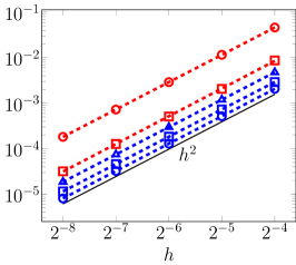
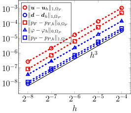
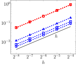
Figure 4.1: Error convergence of the finite element approximation of (2.5) with the manufactured solution (4.1) using (left) $\text{TH}_{1}$, (center) $\text{TH}_{2}$ and (right) CR families for discretization. Optimal convergence is observed in all cases. The legend is shared between the subplots.

Having defined suitable finite element discretization for the Biot-Stokes system, we next investigate robustness of the fractional preconditioner (3.12) which was established theoretically in Theorem 3.1 with the assumption of specific boundary conditions on the sub-boundaries intersecting the interface, namely, that $\Sigma$ meets the intersection between the Biot displacement and the Stokes velocity boundaries. However, the theory and in turn the $\mathcal{R}$ preconditioners can be extended to more general boundary conditions as we will demonstrate by the numerical experiments. In particular, in Section 4.4 we consider the setup where the interface intersects boundaries $\Gamma^{\boldsymbol{\sigma}}_{F}$, $\Gamma^{p_{P}}_{P}$ see Figure 1.1. Then, in Section 4.6 the interface is a closed curve.

Due to the Laplace operator on the interface, the discretization of preconditioners $\mathcal{R}$ (3.12) is not immediately evident. Before discussing the results let us therefore comment on the construction of the critical component, that is, the fractional operators.

4.2 Discrete preconditioner

From (3.12) we observe that in the pressure block of the preconditioner $\mathcal{R}$ the operator acting on $(\varphi,p_{P})$,

$$\begin{pmatrix}\bigl{(}\frac{1}{\lambda}+\frac{1}{2\mu_{s}}\bigr{)}I&-\frac{\alpha}{\lambda}I\\ -\frac{\alpha}{\lambda}I&\bigl{(}C_{0}+\frac{\alpha^{2}}{\lambda}\bigr{)}I-\frac{\kappa}{\mu_{f}}\Delta+\mu^{-1}(-\Delta_{\Sigma,01})^{-\frac{1}{2}}\\ \end{pmatrix}^{-1},$$ (4.2)

contains a sum of a bulk term coupling the two pressures and a fractional interface term $\mu^{-1}(-\Delta_{\Sigma,01})^{-1/2}$. Thus, the action of the operator implicitly involves the trace of the Biot pressure at the interface $\Sigma$. In the discrete setting mirroring this property requires a discrete trace space $S_{h}$ and a restriction operator. In the following we choose $S_{h}$ as the space of piecewise continuous polynomials of order $k+1$ whenever the $\text{TH}_{k}$ family is used. For the CR family, $S_{h}$ is constructed from piecewise continuous linear functions. The restriction operator is then realized as an $L^{2}$-projection.

Once on the interface we approximate the fractional operator based on the spectral decomposition, see, e.g., [45]. That is,

$$\langle\mu^{-1}(-\Delta_{\Sigma,01})^{-1/2}u,v\rangle_{\Sigma}:=\sum_{i}\lambda^{-1/2}_{i}(\mu^{-1}u_{i},u)_{\Sigma}(\mu^{-1}u_{i},v)_{\Sigma}\quad\forall u,v\in S_{h},$$ (4.3)

where $(u_{i},\lambda_{i})\in S_{h}\times\mathbb{R}$ are solutions of the generalized eigenvalue problem

$$(\mu^{-1}\nabla u_{i},\nabla v)_{\Sigma}=\lambda_{i}(\mu^{-1}u_{i},v)_{\Sigma}\quad\forall v\in S_{h},$$ (4.4)

satisfying the orthogonality condition $(\mu^{-1}u_{i},u_{j})_{\Sigma}=\delta_{ij}$. Note that in (4.4) the Dirichlet boundary conditions are prescribed on $\partial\Sigma$ reflecting the trace spaces of velocity and displacement when $\Gamma^{\boldsymbol{u}}_{F}$ and $\Gamma^{\boldsymbol{d}}_{P}$ are incident to $\Sigma$ (as was assumed in Theorem 3.1).

Going beyond the theoretical analysis, we demonstrate in Section 4.4 that for the configuration with $\Gamma^{\boldsymbol{\sigma}}_{F}$, $\Gamma^{p_{P}}_{P}$ intersected by the interface, the operator (4.2) (and in turn the preconditioner (3.12)) needs to be modified. Specifically, the fractional term then reads $\mu^{-1}(-\Delta_{\Sigma}+I_{\Sigma})^{-1/2}$. The operator is defined analogously to (4.3), where, in contrast, the $H^{1}$-norm (cf. the $H^{1}$-seminorm in (4.4)) is now used in the eigenvalue problem: Find $(u_{i},\lambda_{i})\in(S_{h},\mathbb{R})$ such that

$$(\mu^{-1}\nabla u_{i},\nabla v)_{\Sigma}+(\mu^{-1}u_{i},v)_{\Sigma}=\lambda_{i}(\mu^{-1}u_{i},v)_{\Sigma}\quad\forall v\in S_{h}$$ (4.5)

and $(\mu^{-1}u_{i},u_{j})_{\Sigma}=\delta_{ij}$. Note that here the Neumann boundary conditions are prescribed on $\partial\Sigma$.

We remark that the fractional operators and in particular the boundary conditions in (4.4) and (4.5) must be set based on the configuration of the boundaries with respect to the interface. The fact that the conditions cannot be chosen freely is investigated next in Example 4.1 together with the observation that parameter stability of the preconditioners (3.12) is affected by enforcement of Dirichlet boundary conditions in construction of the fractional operators via the eigenvalue problems (4.4) and (4.5).

Example 4.1 (Boundary conditions in fractional operators).

In the following, given the geometry of Example 2.1, let $C_{0}=0$, $\kappa=10^{-10}$ while the remaining problem parameters of the the Biot-Stokes system (2.5) are set to unity. This choice is made to put emphasis on the fractional term in the preconditioner (3.12).

Assuming first that $\Sigma$ intersects $\Gamma^{\boldsymbol{\sigma}}_{F}$ and $\Gamma^{p_{P}}_{P}$, we consider (2.5) either with a preconditioner (3.12), where Dirichlet boundary conditions are (strongly) enforced on the fractional operator, or a modified preconditioner which uses the operator $\mu^{-1}(-\Delta_{\Sigma}+I_{\Sigma})^{-1/2}$ constructed with the Neumann boundary conditions, see (4.5). Using a discretization by $\text{TH}_{1}$ we observe in Table 4.1 that the Dirichlet conditions result in a lack of boundedness in the mesh size. On the other hand, when Neumann boundary conditions are imposed on the fractional operator the spectral condition numbers of the preconditioned problem seem to converge along with mesh refinement.

Repeating the experiment for the configuration where the interface is incident to $\Gamma^{\boldsymbol{u}}_{F}$ and $\Gamma^{\boldsymbol{d}}_{P}$, it can be seen that Neumann boundary conditions lead to a growth similar to what was observed in the previous setup with Dirichlet datum. Furthermore, in Table 4.1 the condition numbers blow up also with $\mu^{-1}(-\Delta_{\Sigma,01})^{-1/2}$. However, in this case the growth can be traced to the (two) eigenvalues that correspond to the degrees of freedom of the space $S_{h}$ on $\partial\Sigma$ which are set strongly by the Dirichlet boundary conditions. This observation motivates using the Nitsche technique [46] in order to enforce the conditions on $\mu^{-1}(-\Delta_{\Sigma,01})^{-1/2}$. With a suitably chosen Nitsche penalty parameter, Table 4.1 (column D_Nitsche) reveals that (3.12) yields mesh independence.

The fact that for $\Sigma$ intersecting $\Gamma^{\boldsymbol{u}}_{F}$ and $\Gamma^{\boldsymbol{d}}_{P}$ the numerical issues with Dirichlet boundary conditions of the fractional operators are related to their strong enforcement, can be further illustrated using a discretization for which the intermediate trace space $S_{h}$ has no degrees of freedom on the boundary $\partial\Sigma$. To this end, we here consider a modification of the CR family where the Biot fluid pressure space is made of piecewise constants. The discrete Laplace operator in (2.5) as well as in the eigenvalue problem (4.4) is then defined analogously to the finite volume method, and in particular utilizing two-point flux approximation, see, e.g., [47]. After using $\mu^{-1}(-\Delta_{\Sigma,01})^{-1/2}$ with Dirichlet boundary conditions enforced weakly, stable condition numbers are achieved, as observed in column $\text{CR}^{\sharp}$ of Table 4.1.

In order to show that strong enforcement of the Dirichlet boundary conditions can be used depending on the boundary configuration, we finally consider a setup where the interface meets $\Gamma^{\boldsymbol{u}}_{F}$ on the Stokes side while on the incident Biot boundary (which we denote by $\Gamma^{\dagger}_{P}$) we assume Dirichlet data on the displacement $\boldsymbol{d}$ and on the pressure $p_{P}$. Then, using a $\text{TH}_{1}$ discretization together with the preconditioner (3.12), bounded condition numbers are produced, which can be observed in the last column of Table 4.1.

$\log_{2}h^{-1}$	$\Gamma^{\boldsymbol{\sigma}}_{F},\Gamma^{p_{P}}_{P}$		$\Gamma^{\boldsymbol{u}}_{F},\Gamma^{\boldsymbol{d}}_{P}$				$\Gamma^{\boldsymbol{u}}_{F},\Gamma^{\dagger}_{P}$
	D	N	D	N	DNitsche	D with $\text{CR}^{\sharp}$	D
2	10.61	16.67	3369	24.48	7.02	8.07	6.77
3	12.17	17.58	13879	30.29	7.43	8.45	7.31
4	13.90	18.12	56254	35.91	7.59	8.60	7.53
5	15.73	18.53	–	41.66	7.67	8.60	7.64
6	17.63	18.83	–	47.66	7.71	8.57	7.69
7	19.58	19.06	–	53.96	7.72	8.54	7.71

Table 4.1: Spectral condition numbers for the Biot-Stokes problem (2.6) with fractional preconditioners (3.12). Boundary condition configurations from Figure 1.1 are considered; $\Sigma$ intersects $\Gamma^{\boldsymbol{\sigma}}_{F}$ and $\Gamma^{p_{P}}_{P}$ or $\Gamma^{\boldsymbol{u}}_{F}$ and $\Gamma^{\boldsymbol{d}}_{P}$. In addition, on $\Gamma^{\dagger}_{P}$ we prescribe both $\boldsymbol{d}$ and $p_{P}$. The fractional preconditioners differ by the boundary conditions enforced on $\partial\Sigma$; Dirichlet condition, cf. (4.4), enforced strongly (D) or with Nitsche’s method (D_Nitsche) or Neumann condition (N), cf. (4.5). Systems are discretized by $\text{TH}_{1}$ family except for $\text{CR}^{\sharp}$ where the modified CR family is used with the Biot pressure space constructed from piecewise constant functions. For the finest refinement level the discrete linear system contains approximately 350 thousand degrees of freedom.

We finally remark that the spectral realization (4.3) is not scalable to problems where the interface and the trace space are large. However, the representation is well suited for the applications pursued here, specifically the robustness study where we are interested in exact (inverted by LU) preconditioners.

4.3 Parameter sensitivity

We demonstrate robustness of the fractional preconditioner (3.12) by a sensitivity study where the physical parameters in (2.5) are varied such that $10^{-9}\leq\mu_{f},\kappa\leq 1$, $1\leq\lambda\leq 10^{12}$, $10^{-2}\leq\gamma\leq 10^{2}$, $10^{-8}\leq\alpha\leq 1$. Since $\mu_{s}$ is commonly used for rescaling we fix its value to 1. Moreover, the storage capacity is set to 0 as this is the more challenging limit of the parameter’s range. The Biot-Stokes system is then considered on the geometry from Example 2.1 with the boundary configuration satisfying the assumptions in Theorem 3.1. That is, the interface intersects $\Gamma^{\boldsymbol{u}}_{F}$ on the Stokes side and $\Gamma^{\boldsymbol{d}}_{P}$ on the Biot side. In turn, the fractional operator is constructed as given in (4.3). Finally, following Example 2.1, the convergence criterion for the MinRes solver is a reduction of the preconditioned residual norm by factor $10^{8}$. The action of the preconditioner (3.12) is then computed by LU factorization of the $2\times 2$ velocity-displacement and the $3\times 3$ pressure blocks, respectively.

Using $\text{TH}_{1}$ elements, Figures 4.2 and 4.3 present slices of the explored parameter space. More precisely, in each subplot column-indexed by fixed value of $\mu_{f}$ and row-indexed by scalar permeability $\kappa$ we plot dependence of the MinRes iterations on system size for varying Lamé parameter $\lambda$ (indicated by color), the Biot-Willis coefficient $\alpha$ (in Figure 4.2, $\gamma$ is set to 1) and the slip-rate coefficient $\gamma$ (in Figure 4.3, $\alpha$ is set to 1). We observe that the iterations are stable for all the parameter combinations. In fact, the iterations remain bounded between $21$-$56$ across the entire considered parameter range.

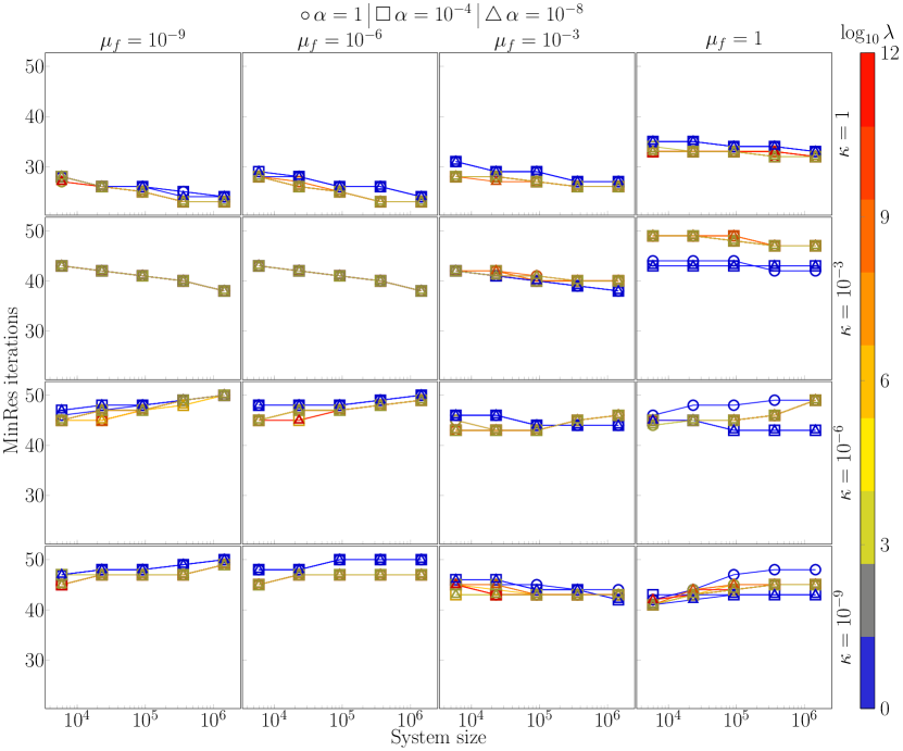
Figure 4.2: Performance of the Biot-Stokes preconditioner (3.12). Geometry of Example 2.1 is used with $\Sigma$ intersecting $\Gamma^{\boldsymbol{u}}_{F}$ and $\Gamma^{\boldsymbol{d}}_{P}$. We set $\mu_{s}$, $\gamma$ to 1 while $C_{0}=0$. The parameters $\mu_{f}$, $\kappa$, $\lambda$, $\alpha$ are varied. Values of the Biot-Willis coefficient are indicated by markers. In this case, the discretization uses $\text{TH}_{1}$ elements.

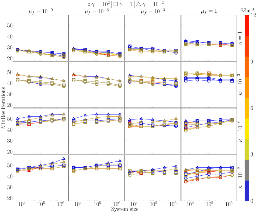
Figure 4.3: Performance of the Biot-Stokes preconditioner (3.12). The problem is setup on the geometry from Example 2.1 with boundary conditions prescribed such that $\Sigma$ intersects $\Gamma^{\boldsymbol{u}}_{F}$ and $\Gamma^{\boldsymbol{d}}_{P}$. We set $\mu_{s}$, $\alpha$ to 1 while $C_{0}=0$. Parameters $\mu_{f}$, $\kappa$, $\lambda$, $\gamma$ are varied. Values of the slip-rate coefficient $\gamma$ are indicated by markers. A discretization by $\text{TH}_{1}$ is used.

4.4 Other boundary configurations

The Biot-Stokes preconditioner (3.12) can be extended beyond the boundary configurations assumed in the theoretical analysis, namely, the requirement that $\Sigma$ is incident to $\Gamma^{\boldsymbol{u}}_{F}$ and $\Gamma^{\boldsymbol{d}}_{P}$. We illustrate this here by letting the interface intersect the boundaries $\Gamma^{\boldsymbol{\sigma}}_{F}$, $\Gamma^{p_{P}}_{P}$. Following Section 4.2, the configuration leads to the fractional operator $\mu^{-1}(-\Delta_{\Sigma}+I_{\Sigma})^{-1/2}$, see (4.5).

Employing the experimental setup of Section 4.3 the performance of the (4.5)-adapted preconditioner (3.12) is illustrated in Figure 4.4 where the slice of the parameter space for $C_{0}=0$, $\gamma=1$ is shown (cf. Figure 4.2 where $\Gamma$ is incident to $\Gamma^{\boldsymbol{u}}_{F}$ and $\Gamma^{\boldsymbol{d}}_{P}$). Using the preconditioner the iterations remain bounded between $23$ and $58$.

For CR family, the MinRes iterations are reported in Figure B.2. Here, for the sake of brevity we present results only for the stronger tangential coupling, i.e. $\gamma$ is fixed at $10^{2}$ and we explore robustness for varying $\mu_{f}$, $\kappa$, $\lambda$ and $\alpha$. It can be seen that the fractional preconditioner leads to bounded iterations (between $22$ and $57$ iterations are required for convergence). We remark that the stability of CR discretization for the three-field Biot formulation is explored in B.

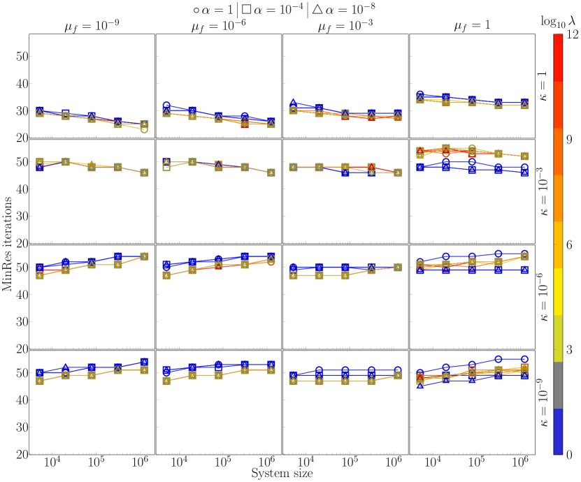
Figure 4.4: Performance of the Biot-Stokes preconditioner (3.12). Geometry of Example 2.1 is used with $\Sigma$ intersecting $\Gamma^{\boldsymbol{\sigma}}_{F}$ and $\Gamma^{p_{P}}_{P}$. The fractional operator is changed to $\mu^{-1}(-\Delta_{\Sigma}+I_{\Sigma})^{-1/2}$. We set $\mu_{s}$, $\gamma$ to 1 while $C_{0}=0$. The parameters $\mu_{f}$, $\kappa$, $\lambda$, $\alpha$ are varied. Values of the Biot-Willis coefficient are indicated by markers. In this case, the discretization uses $\text{TH}_{1}$ elements.

4.5 Diagonal pressure preconditioner

From the point of view of computational efficiency a possible drawback of preconditioner (3.12), is the fact that due to the $C$-seminorm in (3.1) the pressure block contains a $2\times 2$ operator (4.2). However, for the three-field Biot problem, the authors in [27] show that parameter robustness can be obtained also if $(\varphi,p_{P})$ are controlled in a simpler norm, cf. the Biot block of the operator $\mathcal{R}_{D}$ in (2.8). Following this observation we next consider a Biot-Stokes preconditioner of the form

$$\tilde{\mathcal{R}}=\left(\begin{array}[]{cc:ccc}\!\!\!\!\mathcal{A}_{FF}&\!\!\mathcal{A}_{FP}\!\!&&&\\ \!\!\!\!\mathcal{A}_{PF}&\!\!\mathcal{A}_{PP}\!\!&&&\\[2.15277pt] \hdashline\\[-6.45831pt] &&\frac{1}{2\mu_{f}}I&&\\ &&&\!\!\!\!\!\!\bigl{(}\frac{1}{\lambda}+\frac{1}{2\mu_{s}}\bigr{)}I&\\ &&&&\!\!\!\!\!\!\!\bigl{(}C_{0}+\frac{\alpha^{2}}{\lambda}\bigr{)}I-\frac{\kappa}{\mu_{f}}\Delta+\frac{1}{\mu}(-\Delta_{\Sigma,01})^{-\frac{1}{2}}\!\!\!\!\end{array}\right)^{-1},$$ (4.6)

and we note that the pressure block is diagonal.

Using the computational setup of Section 4.3 we compare the preconditioner (3.12) derived in Theorem 3.1 with the [27]-inspired operator $\tilde{\mathcal{R}}$ (4.6). For the simple geometry of Example 2.1 the operators are compared in Figure 4.5. We observe that the preconditioners yield practically identical number of MinRes iteration counts, except for $\lambda=1$, $\alpha=1$ where (4.6) requires more iterations for convergence.

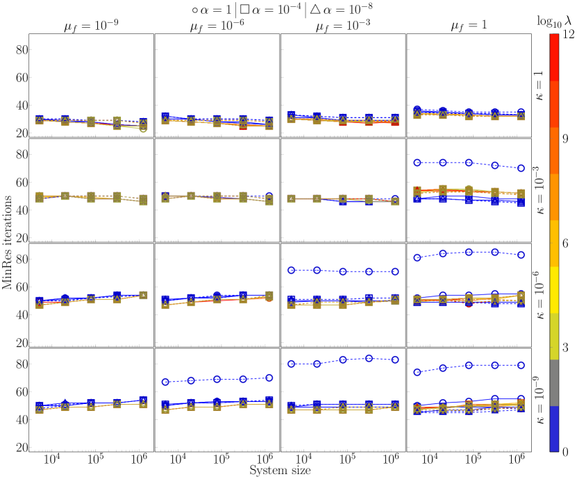
Figure 4.5: Comparison of Biot-Stokes preconditioners (3.12) (solid lines) and (4.6) (dashed lines). Geometry of Example 2.1 is used with $\Sigma$ intersecting $\Gamma^{\boldsymbol{\sigma}}_{F}$ and $\Gamma^{p_{P}}_{P}$. The fractional operator in both preconditioners is changed to $\mu^{-1}(-\Delta_{\Sigma}+I_{\Sigma})^{-1/2}$. We set $\mu_{s}$, $\gamma$ to 1 while $C_{0}=0$. The parameters $\mu_{f}$, $\kappa$, $\lambda$, $\alpha$ are varied. Values of the Biot-Willis coefficient are indicated by markers. The system is discretized by $\text{TH}_{1}$ elements.

4.6 Interfacial flow in the brain

In the examples presented thus far the fractional preconditioners were applied to the Biot-Stokes problem posed in geometries where the interface formed a simple curve (a straight segment in fact). In addition, the number of degrees of freedom associated with $\Sigma$, and in turn the discrete fractional operators, were small.

To apply the proposed fractional preconditioners in a more practical setting our final example concerns the interfacial flow in a brain. As realistic brain geometries currently cannot be tackled with our approach (4.3) due to the size of the interface we choose the problem geometry as two-dimensional slices, see Figure 4.6, left panels. We then model flow of a water-like fluid in free-flow domain that is the space surrounding the brain known as the subarachnoid space and in the poroelastic domain that is the brain parenchyma. We remark that the interface thus forms a closed surface. The material parameters of the Biot model are set following [48] and we fix the slip-rate coefficient as $\gamma=1$. The boundary of the outer spaces is assumed impermeable with $\boldsymbol{u}=\boldsymbol{0}$ prescribed on most of the surface, except for regions (marked with red and orange in Figure 4.6, left) where traction is set in order to drive the flow.

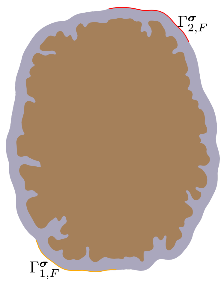
$h\left[\text{mm}\right]$	$\lvert\mathbf{H}_{\epsilon,h}\rvert$	$\lvert S_{h}\rvert$	$\mathcal{R}$	$\mathcal{R}_{D}$	$\mathcal{R}_{C}$
4.72	5114	134	65	369	82
3.21	12919	266	77	445	98
1.93	41545	530	75	473	104
1.05	134980	1066	81	513	114
0.53	482371	2118	83	525	119
0.27	1840764	4234	82	521	119

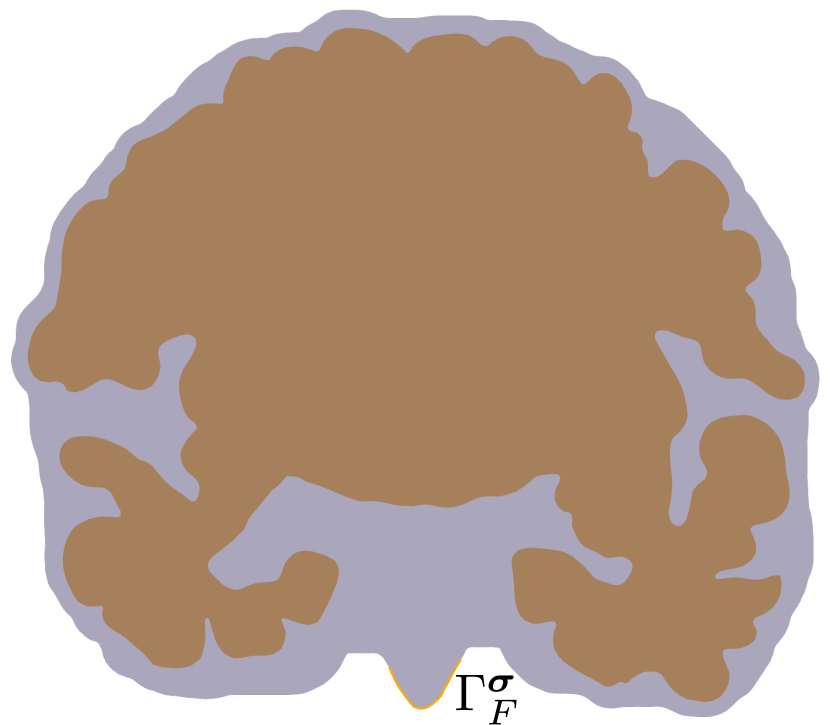
$h\left[\text{mm}\right]$	$\lvert\mathbf{H}_{\epsilon,h}\rvert$	$\lvert S_{h}\rvert$	$\mathcal{R}$	$\mathcal{R}_{D}$	$\mathcal{R}_{C}$
2.46	11681	178	81	413	101
1.67	36677	355	85	458	113
0.86	132775	710	91	494	126
0.44	496680	1420	91	507	131
0.21	1895459	2838	93	511	134

Figure 4.6: Idealized brain sized geometry. The brain is enclosed in a water-filled fluid space. For horizontal slice (top) $\lvert\Sigma\rvert\approx 690\text{mm}$, $\lvert\Gamma^{\boldsymbol{u}}_{F}\rvert\approx 391\text{mm}$, $\lvert\Gamma^{\boldsymbol{\sigma}}_{F}\rvert\approx 140\text{mm}$ while in coronal slice (bottom) $\lvert\Sigma\rvert\approx 825\text{mm}$, $\lvert\Gamma^{\boldsymbol{u}}_{F}\rvert\approx 440\text{mm}$, $\lvert\Gamma^{\boldsymbol{\sigma}}_{F}\rvert\approx 24\text{mm}$. The outer boundary of the fluid space is assumed impermeable except for orange and red segments that form $\Gamma^{\boldsymbol{\sigma}}_{F}$. Gradually refined meshes of the geometry are generated with mesh size in mm given in the $h$ column of the table. The dimensionalities of the corresponding finite element solution space based on $\text{TH}_{1}$ elements are shown together with the size of the trace space $S_{h}$, cf. Section 4.2. The fractional preconditioner (3.12) leads to bounded iterations, and also fewer iterations are required compared to the simple preconditioners from Example 2.1.

Having discretized the system by $\text{TH}_{1}$ elements, the flow problem is solved by a preconditioned MinRes solver starting from a 0 initial vector with relative tolerance of $10^{-8}$. As the preconditioner (3.12) is used, where the fractional term reads $\mu^{-1}(-\Delta_{\Sigma}+I_{\Sigma})^{-1/2}$, cf. Section 4.4. Note that, while $\Sigma$ is now a closed surface, the fractional operator is well defined (and invertible) as the spectrum of the eigenvalue problem (4.5) is positive due to the $H^{1}$-inner product used in the definition.

The number of iterations required for convergence is tabulated in Figure 4.6, right. The iterations are bounded in mesh size and (while the interface is more complex and the interface problem much larger) are in fact comparable to those in the simple setup of Example 2.1 and Section 4.3. We note that the fractional preconditioner leads to faster convergence of the MinRes solver especially compared to the simple block-diagonal preconditioner $\mathcal{R}_{D}$, see Example 2.1.

The resulting flow and pressure fields for the two sets of simulations are shown in Figure 4.7, exhibiting localization of pressure, permeating into the porous domain following the directions dictated by the brain displacement.

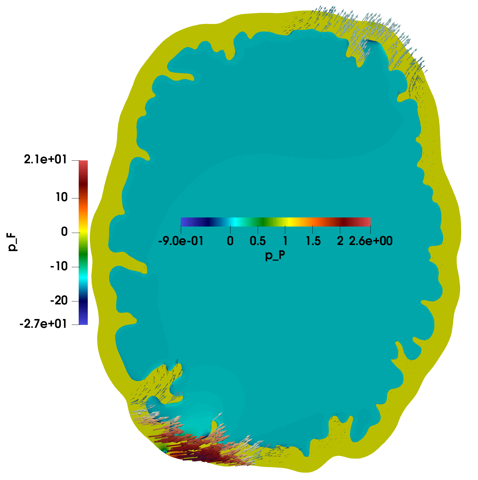
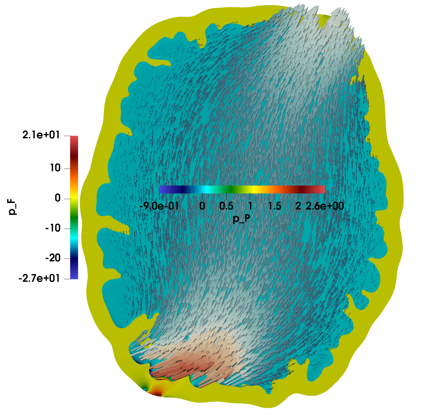
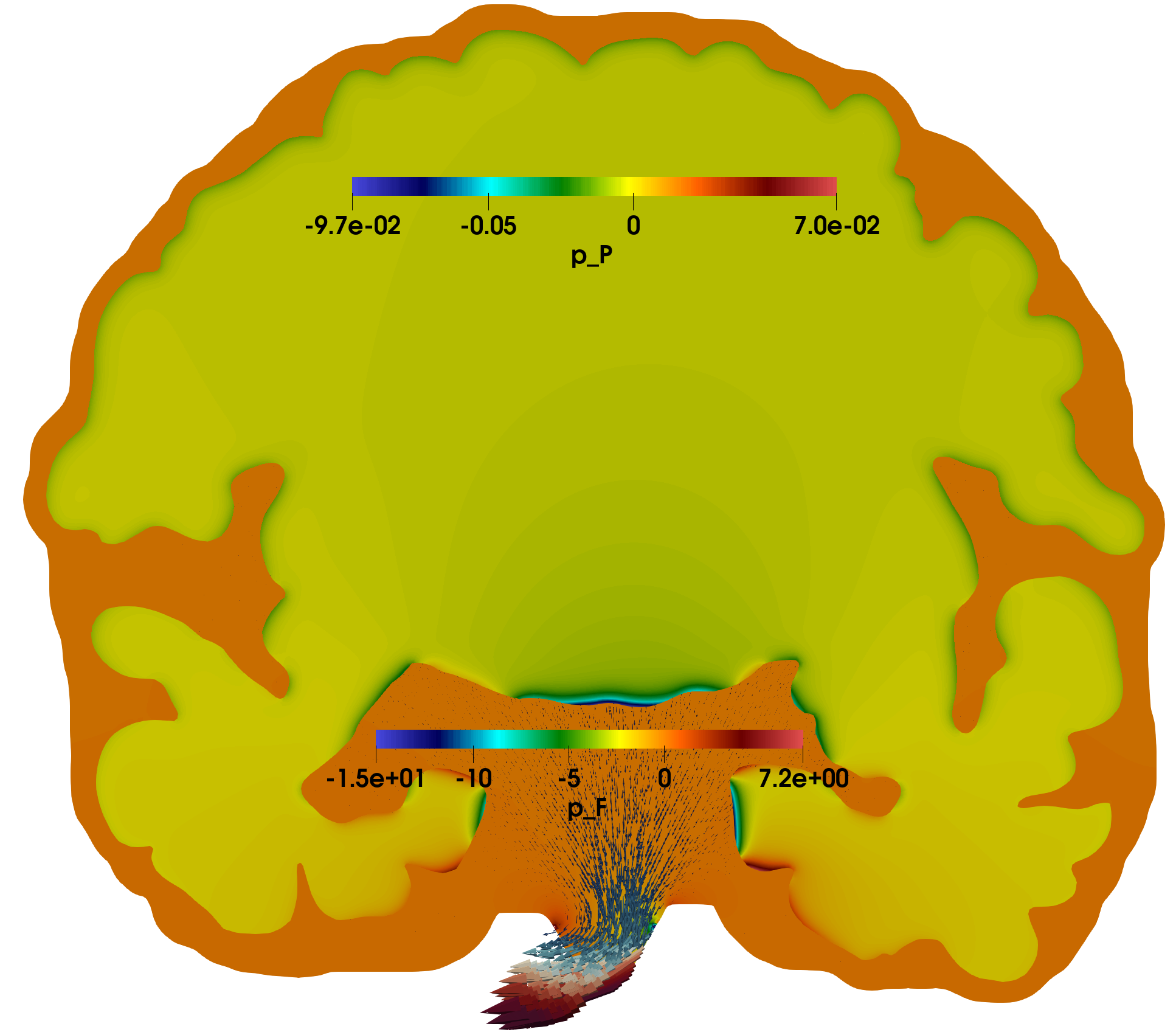
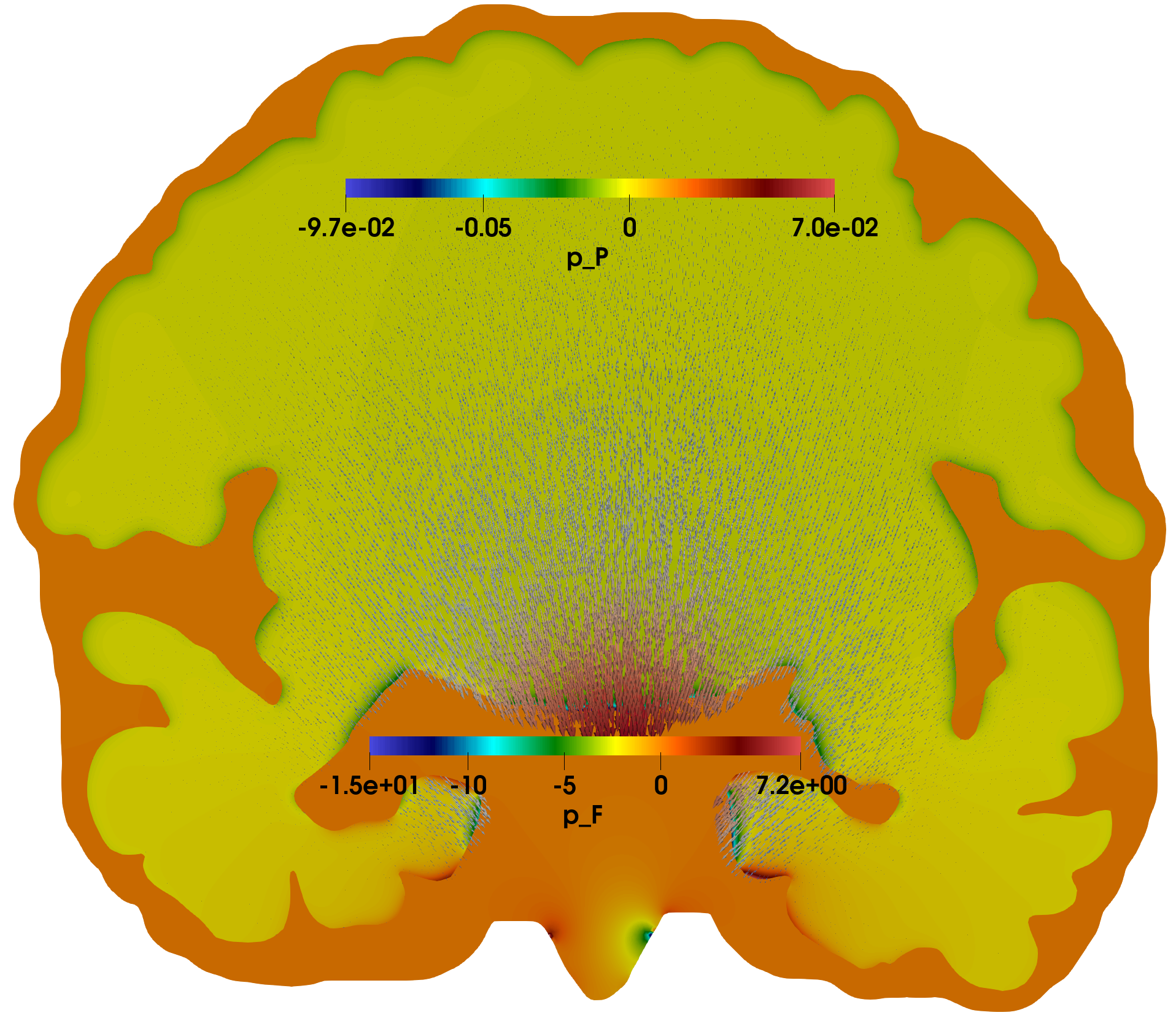
Figure 4.7: Interfacial flow in an idealized geometry. The traction boundary conditions in the top right and bottom left corners (horizontal slices), respectively at the bottom (coronal slices), induce the fluid flow (left) and the brain displacement (right).

Appendix A TH_k and CR finite element families

We denote by $\{\mathcal{T}_{h}\}_{h>0}$ a shape-regular family of partitions of $\bar{\Omega}$, conformed by tetrahedra (or triangles in 2D) $K$ of diameter $h_{K}$, with mesh size $h:=\max\{h_{K}:\;K\in\mathcal{T}_{h}\}$, and denote $\mathcal{T}_{h}^{F}$ and $\mathcal{T}_{h}^{P}$ the restrictions of the mesh elements to the subdomains $\Omega_{F}$ and $\Omega_{P}$, respectively. Similarly, by $\mathcal{E}_{h}^{F}$ and $\mathcal{E}_{h}^{P}$ we will denote the restrictions to the mesh facets (edges in 2D) to the Stokes and Biot subdomains, respectively. We assume that the two partitions match at the interface. Given an integer $k\geq 1$ and a subset $S$ of $\mathbb{R}^{d}$, $d=2,3$, by $\mathbb{P}_{k}(S)$ we will denote the space of polynomial functions defined locally in $S$ and being of total degree up to $k$. The methods that we use are based on the generalized Taylor-Hood [49] and Crouzeix-Raviart [50] finite element families that give an overall $k+1$ order of convergence

$$\mathrm{TH}_{k} \begin{cases}\vec{\mathbf{V}}_{h}=\{(\boldsymbol{v}_{h},\boldsymbol{w}_{h})\!\in\!\vec{\mathbf{V}}\!:\boldsymbol{v}_{h}|_{K}\in\mathbb{P}_{k+1}(K)^{d},\boldsymbol{w}_{h}|_{L}\in\mathbb{P}_{k+1}(L)^{d},\forall K\in\mathcal{T}^{F}_{h},L\in\mathcal{T}_{h}^{P}\},\\ \vec{Q}_{h}=\{\vec{q}_{h}\in\vec{Q}\cap[C(\Omega_{F})\times C(\Omega_{P})\times L^{2}(\Omega_{P})]:\\ \qquad\ q_{F,h}|_{K}\in\mathbb{P}_{k}(K),\psi_{h}|_{L}\in\mathbb{P}_{k}(L),q_{P,h}|_{L}\in\mathbb{P}_{k+1}(L),\forall K\in\mathcal{T}^{F}_{h},L\in\mathcal{T}_{h}^{P}\},\end{cases}$$

$$\mathrm{CR} \begin{cases}\vec{\mathbf{V}}_{h}=\{(\boldsymbol{v}_{h},\boldsymbol{w}_{h})\!\in\!\mathbf{L}^{2}(\Omega_{F})\times\mathbf{L}^{2}(\Omega_{P})\!:\boldsymbol{v}_{h}|_{K}\in\mathbb{P}_{1}(K)^{d},\boldsymbol{w}_{h}|_{L}\in\mathbb{P}_{1}(L)^{d},\\ \quad\quad\int_{e}[\![\boldsymbol{v}_{h}\cdot\boldsymbol{n}_{e}]\!]=0,\ \int_{\ell}[\![\boldsymbol{w}_{h}\cdot\boldsymbol{n}_{\ell}]\!]=0\ \forall e\subset\partial K,\ell\subset\partial L,\,K\in\mathcal{T}^{F}_{h},L\in\mathcal{T}_{h}^{P}\},\\ \vec{Q}_{h}=\{\vec{q}_{h}\in\vec{Q}\cap[L^{2}(\Omega_{F})\times L^{2}(\Omega_{P})\times C(\Omega_{P})]:q_{F,h}|_{K}\in\mathbb{P}_{0}(K),\\ \quad\quad\psi_{h}|_{L}\in\mathbb{P}_{0}(L),q_{P,h}|_{L}\in\mathbb{P}_{1}(L),\forall K\in\mathcal{T}^{F}_{h}\!,L\in\mathcal{T}_{h}^{P}\}.\end{cases}$$

Appendix B CR discretization for Biot system

We investigate numerically the stability of the three-field (total pressure) formulation of Biot equations discretized by the CR family. Assuming momentarily that $\partial\Omega_{P}=\Gamma^{\boldsymbol{d}}_{P}$ the discrete weak problem reads: Find $(\boldsymbol{d}_{h},p_{P,h},\varphi_{h})\in\mathbf{W}_{h}\times Q^{P}_{h}\times Z_{h}$ such that for all $(\boldsymbol{w}_{h},q_{P,h},Z_{h})\in\mathbf{W}_{h}\times Q^{P}_{h}\times Z_{h}$ it holds that

$$\int_{\Omega_{P}}2\mu_{s}\boldsymbol{\epsilon}(\boldsymbol{d}_{h}):\boldsymbol{\epsilon}(\boldsymbol{w}_{h})+\int_{\mathcal{E}_{h}^{P}}\frac{2\mu_{f}}{h}[\![\boldsymbol{d}_{h}\cdot\boldsymbol{n}]\!][\![\boldsymbol{w}_{h}\cdot\boldsymbol{n}]\!]-\int_{\Omega_{P}}\varphi_{h}\mathop{\mathrm{div}}\nolimits\boldsymbol{w}_{h} =\int_{\Omega_{P}}\boldsymbol{f}\cdot\boldsymbol{w}_{h},$$ (B.1)

$$-\int_{\Omega_{P}}\frac{\alpha^{2}}{\lambda}p_{P,h}q_{P,h}-\int_{\Omega_{P}}\frac{\kappa}{\mu_{f}}\nabla p_{P,h}\cdot\nabla q_{P,h}+\int_{\Omega_{P}}\frac{\alpha}{\lambda}\varphi_{h}q_{P,h} =0,$$

$$\int_{\Omega_{P}}\psi_{h}\left(-\mathop{\mathrm{div}}\nolimits\boldsymbol{d}_{h}+\frac{\alpha}{\lambda}p_{P,h}-\frac{1}{\lambda}\varphi_{h}\right) =0.$$

Note that the momentum balance equation includes a stabilization as described in [41].

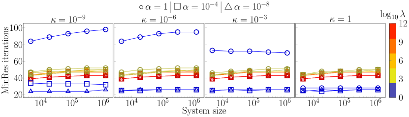
Figure B.1: Total pressure Biot formulation (B.1) with preconditioner from [27], and using a discretization by CR family.

In Figure B.1 we report the number of iterations required for convergence of MinRes solver started from random initial vector until reducing the preconditioned residual norm by a factor of $10^{8}$. Here the preconditioner analyzed in [27] (that is, the preconditioner is formed by the second, fourth and final blocks of the operator $\mathcal{R}_{D}$ in (2.8)) is used. We remark that in the numerical experiment $\Omega_{P}=(0,1)^{2}$, and $\lvert\Gamma^{p_{P}}_{P}\rvert\cdot\lvert\Gamma^{\boldsymbol{d}}_{P}\rvert>0$. We observe that the iterations are bounded with respect to the mesh size as well as to variations in material parameters.

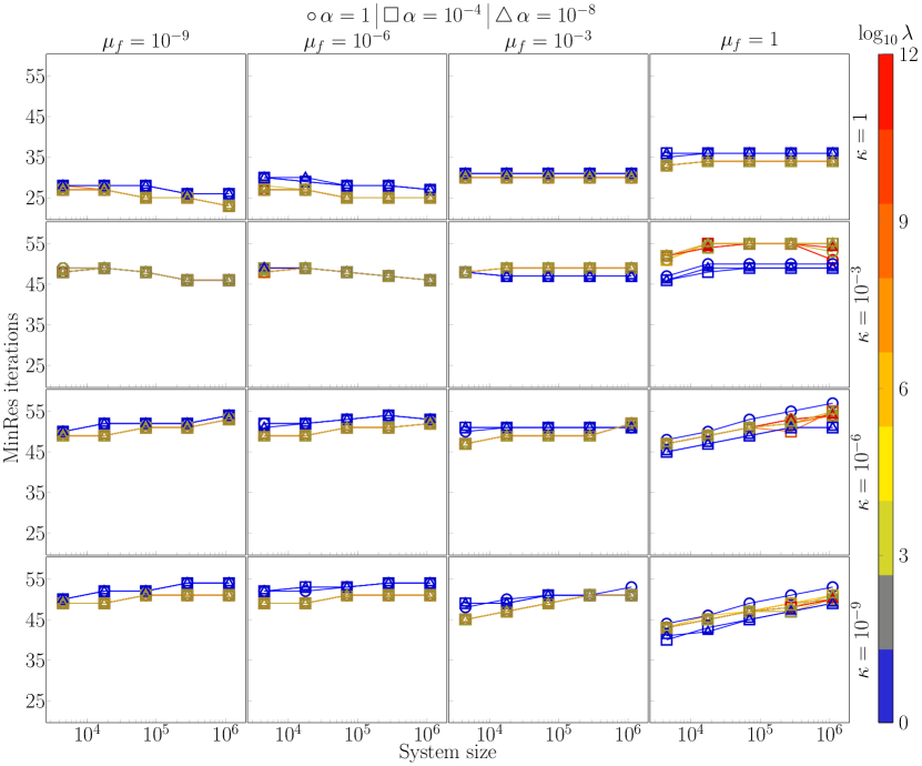
Figure B.2: Performance of Biot-Stokes preconditioner (3.12). Geometry of Example 2.1 is used with $\Sigma$ intersecting $\Gamma^{\boldsymbol{\sigma}}_{F}$ and $\Gamma^{p_{P}}_{P}$. The fractional operator is changed to $\mu^{-1}(-\Delta_{\Sigma}+I_{\Sigma})^{-1/2}$. We set $\mu_{s}=1$, $C_{0}=0$, $\gamma=10^{2}$. The parameters $\mu_{f}$, $\kappa$, $\lambda$, $\alpha$ are varied. Values of the Biot-Willis coefficient are indicated by markers. The discretization is done using the CR family.

References

- [1] M. A. Murad, J. N. Guerreiro, A. F. Loula, Micromechanical computational modeling of secondary consolidation and hereditary creep in soils, Computer Methods in Applied Mechanics and Engineering 190 (15) (2001) 1985–2016.
- [2] R. E. Showalter, Poroelastic filtration coupled to Stokes flow, in: O. Imanuvilov, G. Leugering, R. Triggiani, B.-Y. Zhang (Eds.), Control Theory of Partial Differential Equations, Vol. 242 of Lecture Notes in Pure and Applied Mathematics, Chapman & Hall, Boca Raton, 2005, pp. 229–241.
- [3] E. A. Bergkamp, C. V. Verhoosel, J. J. C. Remmers, D. M. J. Smeulders, A staggered finite element procedure for the coupled Stokes-Biot system with fluid entry resistance, Computational Geosciences 24 (2020) 1497–1522.
- [4] C. Ager, B. Schott, M. Winter, W. A. Wall, A Nitsche-based cut finite element method for the coupling of incompressible fluid flow with poroelasticity, Computer Methods in Applied Mechanics and Engineering 351 (2019) 253–280.
- [5] I. Ambartsumyan, E. Khattatov, I. Yotov, P. Zunino, A Lagrange multiplier method for a Stokes–Biot fluid–poroelastic structure interaction model, Numerische Mathematik 140 (2) (2018) 513 – 553. doi:10.1007/s00211-018-0967-1.
- [6] S. Badia, A. Quaini, A. Quarteroni, Coupling Biot and Navier-Stokes equations for modelling fluid-poroelastic media interaction, Journal of Computational Physics 228 (2009) 7986 – 8014.
- [7] M. Bukač, I. Yotov, R. Zakerzadeh, P. Zunino, Partitioning strategies for the interaction of a fluid with a poroelastic material based on a Nitsche’s coupling approach, Computer Methods in Applied Mechanics and Engineering 292 (2015) 138 – 170.
- [8] S. Caucao, T. Li, I. Yotov, A multipoint stress-flux mixed finite element method for the Stokes-Biot model, arXiv preprint arXiv:2011.01396 (2020).
- [9] A. Cesmelioglu, Analysis of the coupled Navier-Stokes/Biot problem, Journal of Mathematical Analysis and Applications 456 (2) (2017) 970–991.
- [10] A. Cesmelioglu, P. Chidyagwai, Numerical analysis of the coupling of free fluid with a poroelastic material, Numerical Methods for Partial Differential Equations 36 (3) (2020) 463–494.
- [11] T. Li, I. Yotov, A mixed elasticity formulation for fluid-poroelastic structure interaction, arXiv preprint arXiv:2011.00132 (2020).
- [12] M. Taffetani, R. Ruiz-Baier, S. L. Waters, Coupling Stokes flow with inhomogeneous poroelasticity, Quarterly Journal of Mechanics and Applied Mathematics in press (2021).
- [13] J. Wen, Y. He, A strongly conservative finite element method for the coupled Stokes-Biot model, Computers and Mathematics with Applications 80 (2020) 1421–1442. doi:10.1016/j.camwa.2020.07.001.
- [14] J. Wen, J. Su, Y. He, H. Chen, Discontinuous Galerkin method for the coupled Stokes-Biot model, Numerical Methods for Partial Differential Equations 37 (2021) 383–405. doi:10.1002/num.22532.
- [15] H. K. Wilfrid, Nonconforming finite element methods for a Stokes/Biot fluid–poroelastic structure interaction model, Results in Applied Mathematics 7 (2020) 100127. doi:10.1016/j.rinam.2020.100127.
- [16] R. Ruiz-Baier, M. Taffetani, H. D. Westermeyer, I. Yotov, The Biot-Stokes coupling using total pressure: formulation, analysis and application to interfacial flow in the eye, Computer Methods in Applied Mechanics and Engineering under revision (2021).
- [17] I. Ambartsumyan, V. J. Ervin, T. Nguyen, I. Yotov, A nonlinear Stokes-Biot model for the interaction of a non-Newtonian fluid with poroelastic media, ESAIM: Mathematical Modelling and Numerical Analysis 53 (6) (2019) 1915–1955.
- [18] R. Bürger, S. Kumar, D. Mora, R. Ruiz-Baier, N. Verma, Virtual element methods for the three-field formulation of time-dependent linear poroelasticity, Advances in Computational Mathematics 47 (2021) e2(1–37).
- [19] S. Kumar, R. Oyarzúa, R. Ruiz-Baier, R. Sandilya, Conservative discontinuous finite volume and mixed schemes for a new four-field formulation in poroelasticity, ESAIM: Mathematical Modelling and Numerical Analysis 54 (1) (2020) 273–299.
- [20] R. Oyarzúa, R. Ruiz-Baier, Locking-free finite element methods for poroelasticity, SIAM Journal on Numerical Analysis 54 (5) (2016) 2951–2973.
- [21] W. M. Boon, T. Koch, M. Kuchta, K.-A. Mardal, Robust monolithic solvers for the Stokes-Darcy problem with the Darcy equation in primal form, arXiv preprint arXiv2110.07486 (2021).
- [22] P. Chidyagwai, S. Ladenheim, D. B. Szyld, Constraint preconditioning for the coupled Stokes–Darcy system, SIAM Journal on Scientific Computing 38 (2) (2016) A668–A690.
- [23] K. E. Holter, M. Kuchta, K.-A. Mardal, Robust preconditioning for coupled Stokes–Darcy problems with the Darcy problem in primal form, Computers & Mathematics with Applications 91 (2021) 56–66.
- [24] T. Karper, K.-A. Mardal, R. Winther, Unified finite element discretizations of coupled Darcy–Stokes flow, Numerical Methods for Partial Differential Equations 25 (2) (2009) 311–326.
- [25] K.-A. Mardal, R. Winther, Preconditioning discretizations of systems of partial differential equations, Numerical Linear Algebra with Applications 18 (2011) 1–40.
- [26] K.-A. Mardal, M. E. Rognes, T. B. Thompson, Accurate discretization of poroelasticity without Darcy stability, BIT Numerical Mathematics (2021) 1–36.
- [27] J. Lee, K.-A. Mardal, R. Winther, Parameter-robust discretization and preconditioning of Biot’s consolidation model, SIAM Journal on Scientific Computing 39 (1) (2017) A1–A24.
- [28] J. Lee, E. Piersanti, K.-A. Mardal, M. Rognes, A mixed finite element method for nearly incompressible multiple-network poroelasticity, SIAM J. Sci. Comput. 41 (2) (2019) A722–A747.
- [29] W. Boon, M. Kuchta, K.-A. Mardal, R. Ruiz-Baier, Robust preconditioners and stability analysis for perturbed saddle-point problems – application to conservative discretizations of Biot’s equations utilizing total pressure, SIAM Journal on Scientific Computing 43 (4) (2021) B961–B983.
- [30] T. Bærland, M. Kuchta, K.-A. Mardal, T. Thompson, An observation on the uniform preconditioners for the mixed Darcy problem, Numerical Methods for Partial Differential Equations (2020) 1–17.
- [31] J. Bergh, J. Löfström, Interpolation spaces: an introduction, Vol. 223, Springer Science & Business Media, 2012.
- [32] G. N. Gatica, A Simple Introduction to the Mixed Finite Element Method, Springer-Verlag, Berlin, 2014.
- [33] C. le Roux, B. D. Reddy, The steady Navier-Stokes equations with mixed boundary conditions: application to free boundary flows, Nonlinear Analysis. Theory, Methods & Applications. An International Multidisciplinary Journal 20 (9) (1993) 1043–1068. doi:10.1016/0362-546X(93)90094-9.
- [34] D. Braess, Stability of saddle point problems with penalty, ESAIM: Mathematical Modelling and Numerical Analysis-Modélisation Mathématique et Analyse Numérique 30 (6) (1996) 731–742.
- [35] V. Girault, P.-A. Raviart, Finite Element Methods for Navier-Stokes Equations: Theory and Algorithms, 1st Edition, Springer Publishing Company, 1986.
- [36] A. Ern, J.-L. Guermond, Theory and Practice of Finite Elements, Appl. Math. Sci. 159, Springer-Verlag, New York, 2004.
- [37] V. Anaya, A. Khan, D. Mora, R. Ruiz-Baier, Robust a posteriori error analysis for rotation-based formulations of the elasticity/poroelasticity coupling, arXiv preprint arXiv2106.09074 (2021).
- [38] J. Galvis, M. Sarkis, Non-matching mortar discretization analysis for the coupling Stokes-Darcy equations, Electron. Trans. Numer. Anal. 26 (2007) 350–384.
- [39] W. J. Layton, F. Schieweck, I. Yotov, Coupling fluid flow with porous media flow, SIAM Journal on Numerical Analysis 40 (6) (2002) 2195–2218.
- [40] M. Arioli, D. Loghin, Discrete interpolation norms with applications, SIAM Journal on Numerical Analysis 47 (4) (2009) 2924–2951.
- [41] E. Burman, P. Hansbo, Stabilized Crouzeix-Raviart element for the Darcy-Stokes problem, Numerical Methods for Partial Differential Equations 21 (5) (2005) 986–997. doi:https://doi.org/10.1002/num.20076.
- [42] M. S. Alnæs, J. Blechta, J. Hake, A. Johansson, B. Kehlet, A. Logg, C. Richardson, J. Ring, M. E. Rognes, G. N. Wells, The FEniCS project version 1.5, Archive of Numerical Software 3 (100) (2015) 9–23.
- [43] A. Logg, K.-A. Mardal, G. Wells, Automated Solution of Differential Equations by the Finite Element Method, Springer-Verlag, Berlin, Germany, 2012. doi:10.1007/978-3-642-23099-8.
- [44] M. Kuchta, Assembly of multiscale linear PDE operators, in: F. J. Vermolen, C. Vuik (Eds.), Numerical Mathematics and Advanced Applications ENUMATH 2019, Springer International Publishing, Cham, 2021, pp. 641–650.
- [45] M. Kuchta, M. Nordaas, J. Verschaeve, M. Mortensen, K. Mardal, Preconditioners for saddle point systems with trace constraints coupling 2D and 1D domains, SIAM Journal on Scientific Computing 38 (6) (2016) B962–B987.
- [46] J. C. C. Nitsche, Über ein variationsprinzip zur lösung von Dirichlet-problemen bei verwendung von teilräumen, die keinen randbedingungen unterworfen sind, Abhandlungen aus dem Mathematischen Seminar der Universität Hamburg 36 (1971) 9–15.
- [47] J. Droniou, N. Nataraj, Improved estimate for gradient schemes and super-convergence of the TPFA finite volume scheme, IMA Journal of Numerical Analysis 38 (3) (2017) 1254–1293. doi:10.1093/imanum/drx028.
- [48] S. Budday, R. Nay, R. de Rooij, P. Steinmann, T. Wyrobek, T. C. Ovaert, E. Kuhl, Mechanical properties of gray and white matter brain tissue by indentation, Journal of the Mechanical Behavior of Biomedical Materials 46 (2015) 318–330. doi:https://doi.org/10.1016/j.jmbbm.2015.02.024.
- [49] C. Taylor, P. Hood, A numerical solution of the Navier-Stokes equations using the finite element technique, Computers & Fluids 1 (1) (1973) 73–100.
- [50] M. Crouzeix, P.-A. Raviart, Conforming and nonconforming finite element methods for solving the stationary Stokes equations i, ESAIM: Mathematical Modelling and Numerical Analysis-Modélisation Mathématique et Analyse Numérique 7 (R3) (1973) 33–75.