On the geometry of flag Hilbert–Poincaré series for matroids

Abstract.

We extend the definition of coarse flag Hilbert–Poincaré series to matroids; these series arise in the context of local Igusa zeta functions associated to hyperplane arrangements. We study these series in the case of oriented matroids by applying geometric and combinatorial tools related to their topes. In this case, we prove that the numerators of these series are coefficient-wise bounded below by the Eulerian polynomial and equality holds if and only if all topes are simplicial. Moreover this yields a sufficient criterion for non-orientability of matroids of arbitrary rank.

1. Introduction

The flag Hilbert–Poincaré series associated to a hyperplane arrangement, defined in [18], is a rational function in several variables connected to local Igusa zeta functions [6]. In fact, polynomial substitutions of the variables of the flag Hilbert–Poincaré series also yield motivic zeta functions associated to matroids [16]; see [24] for the topological analog. There are also substitutions yielding so-called ask zeta functions associated to certain modules of matrices [22]; see [18, Prop. 4.8]. The analytic and arithmetic properties of these zeta functions are, therefore, heavily influenced by the combinatorics of the flag Hilbert–Poincaré series. Here, we bring in combinatorial tools to better understand features of this series.

We consider a specialization in variables $Y$ and $T$, called the coarse flag Hilbert–Poincaré series, which seems to have remarkable combinatorial properties. In [18], it was shown that for most Coxeter hyperplane arrangements, the numerator of this specialization at $Y=1$ is equal to an Eulerian polynomial. We generalize this to the setting of oriented matroids, a combinatorial abstraction of the face structure determined by real hyperplane arrangements. We show that the numerator can be better understood from the geometry of the topes, which are analogs of the chambers for real hyperplane arrangements. This settles a question by Voll and the second author [18, Quest. 1.7] for the case of real arrangements, asking about which properties of a hyperplane arrangement guarantee the equality to Eulerian polynomials mentioned above.

1.1. Flag Hilbert–Poincaré series for matroids

Let $M$ be a matroid, with ground set $E$, and $\mathcal{L}(M)$ its lattice of flats, with bottom and top elements denoted by $\hat{0}$ and $\hat{1}$, respectively. Relevant definitions concerning matroids and oriented matroids are given in Section 2. Let $\mu_{M}:\mathcal{L}(M)\rightarrow\mathbb{Z}$ be the Möbius function on $\mathcal{L}(M)$, where $\mu_{M}(\hat{0})=1$ and $\mu_{M}(X)=-\sum_{X^{\prime}<X}\mu_{M}(X^{\prime})$. A well-studied invariant of a matroid $M$ is the Poincaré polynomial

$$\pi_{M}(Y) =\sum_{X\in\mathcal{L}(M)}\mu_{M}(X)(-Y)^{r(X)},$$

where $r(X)$ is the rank of $X$ in $\mathcal{L}(M)$, viz. one less than the maximum over the number of elements of all flags from $\hat{0}$ to $X$. If $M$ is realized by a hyperplane arrangement $\mathcal{A}$, then its Poincaré polynomial captures topological and algebraic properties of $\mathcal{A}$ [20].

For a poset $P$ let $\Delta(P)$ be the set of flags of $P$, and let $\Delta_{k}(P)\subseteq\Delta(P)$ be the set of flags of size $k$. If $P$ has a bottom element $\hat{0}$ and a top element $\hat{1}$ set $\overline{P}=P\setminus\{\hat{0},\hat{1}\}$. The flag Poincaré polynomial associated to $F=(X_{1}<\cdots<X_{\ell})\in\Delta(\overline{\mathcal{L}}(M))$, with $\ell\geqslant 0$, is the product of Poincaré polynomials on the minors determined by $F$,

$$\pi_{F}(Y) =\prod_{k=0}^{\ell}\pi_{M/X_{k}|X_{k+1}}(Y),$$

where $X_{0}=\hat{0}$ and $X_{\ell+1}=\hat{1}$. Here, $M/X_{k}$ is the contraction of $X_{k}\subseteq E$ from $M$, and $M|X_{k+1}$ is the restriction of $M$ to $X_{k+1}\subseteq E$. The lattice $\mathcal{L}(M/X_{k}|X_{k+1})$ is isomorphic to the interval $[X_{k},X_{k+1}]$ in $\mathcal{L}(M)$.

Definition 1.1.

The coarse flag Hilbert–Poincaré series of a matroid $M$ is

$$\mathsf{cfHP}_{M}(Y,T) =\dfrac{1}{1-T}\sum_{F\in\Delta(\overline{\mathcal{L}}(M))}\pi_{F}(Y)\left(\dfrac{T}{1-T}\right)^{|F|}=\dfrac{\mathcal{N}_{M}(Y,T)}{(1-T)^{r(M)}}.$$

We call $\mathcal{N}_{M}(Y,T)$ the coarse flag polynomial:

$$\mathcal{N}_{M}(Y,T)=\sum_{F\in\Delta(\overline{\mathcal{L}}(M))}\pi_{F}(Y)T^{|F|}(1-T)^{r(M)-1-|F|}.$$

We call a matroid $M$ orientable if there exists an oriented matroid whose underlying matroid is $M$. An orientable matroid $M$ is simplicial if $M$ has an oriented matroid structure such that the face lattice of every tope is a Boolean lattice—equivalently, for real hyperplane arrangements every chamber is a simplicial cone; see details in Section 2.2. For example, all Coxeter arrangements are simplicial.

1.2. Main results

For rational polynomials $f(T)=\sum_{k\geqslant 0}a_{k}T^{k}$ and $g(T)=\sum_{k\geqslant 0}b_{k}T^{k}$, we write $f(T)\leqslant g(T)$ if $a_{k}\leqslant b_{k}$ for all $k\geqslant 0$. We write $f(T)<g(T)$ to mean $f(T)\leqslant g(T)$ and $f(T)\neq g(T)$.

The Eulerian polynomials $E_{r+1}^{\mathsf{A}}(T)$ and $E_{r+1}^{\mathsf{B}}(T)$ are equal to the $h$-polynomials of the barycentric subdivisions of the boundaries of the $r$-dimensional simplex and the cross-polytope, respectively [21, Thm. 11.3]. The Eulerian polynomials are also defined by Coxeter-theoretic descent statistics [21, Sec. 11.4]. In [18, Thm. D], it was shown that for all Coxeter arrangements $\mathcal{A}$ of rank $r$, without an $\mathsf{E}_{8}$-factor, $\mathcal{N}_{\mathcal{A}}(1,T)/\pi_{\mathcal{A}}(1)=E_{r}^{\mathsf{A}}(T)$. The next theorem generalizes this result.

Theorem 1.2.

Let $M$ be an orientable matroid of rank $r$. Then

(1.1) $$E_{r}^{\mathsf{A}}(T)\leqslant\dfrac{\mathcal{N}_{M}(1,T)}{\pi_{M}(1)},$$

and equality holds if and only if $M$ is simplicial. Moreover,

$$\mathcal{N}_{M}(1,T^{-1}) =T^{r-1}\mathcal{N}_{M}(1,T).$$

The key insight in the proof for Theorem 1.2 is that in the orientable case $\mathcal{N}_{M}(1,T)$ is a sum of $h$-polynomials. Each of the summands is determined by the topes of $M$; see Proposition 4.3. Theorem 1.2 suggests that $\mathcal{N}_{M}(Y,T)$ is a “$Y$-twisted” sum of $h$-polynomials of the topes, and understanding this could address the nonnegativity conjecture of [18] in the orientable case.

A byproduct of Theorem 1.2 is a sufficient condition for non-orientability of matroids. The rank $3$ case yields an inequality concerning the the number of rank $2$ flats above every element in $M$.

Corollary 1.3.

Assume $M$ is a simple matroid with rank $3$, and suppose $c$ is the number of rank $2$ flats of $M$ and $s$ the sum of their sizes. If $3(c-1)<s$, then $M$ is non-orientable.

It is known that the Fano matroid is non-orientable, which is also shown by Corollary 1.3 since it has seven rank $2$ flats, each containing three elements. There are a number of sufficient conditions for the non-orientability of matroids. Based on experiments using the database of non-orientable matroids [19], we report that the condition in Corollary 1.3 is independent from the sufficient condition in [7] for rank $3$ matroids; see also [4, Prop. 6.6.1(i)]. Moreover, Corollary 1.3 is related to Corollary 2.6 in [8] where Cuntz and Geis proved that a rank $3$ arrangement is simplicial if and only if its underlying matroid satisfies $3(c-1)=s$ in the notation above.

1.3. Further questions and conjectures

The lower bound in (1.1) raises the following question. How large or how small can the coefficients of the numerator of $\mathsf{cfHP}_{M}(1,T)/\pi_{M}(1)$ be? All of our results and computations suggest the following.

Conjecture 1.4.

For all matroids $M$ of rank $r\geqslant 3$,

$$(1+T)^{r-1}<\dfrac{\mathcal{N}_{M}(1,T)}{\pi_{M}(1)}<E_{r}^{\mathsf{B}}(T).$$

We note that $E_{1}^{\mathsf{A}}(T)=E_{1}^{\mathsf{B}}(T)=1$ and $E_{2}^{\mathsf{A}}(T)=E_{2}^{\mathsf{B}}(T)=1+T$, and all matroids of rank 1 or 2 are both orientable and simplicial. For orientable matroids, the lower bound of Conjecture 1.4 holds by Theorem 1.2. Moreover, the upper bound in Conjecture 1.4 is reminiscent of similar “$f$-vector” bounds proved in [14, 25].

Theorem 1.5.

1. If Conjecture 1.4 holds, then the bounds are sharp.

2. Conjecture 1.4 holds for all matroids of rank $3$. Moreover for all orientable matroids, the upper bound holds for the linear term of the polynomials, so Conjecture 1.4 holds for all orientable matroids of rank $4$.

In fact, more is known to hold for $\mathcal{N}_{M}(Y,T)$ in the case where $r(M)\leqslant 3$. We prove, in Proposition 3.2, that the numerator is nonnegative, palindromic, and when $Y=1$ real-rooted. In particular, Conjecture E from [18] holds for all central hyperplane arrangements with rank at most $3$. We are also interested in whether or not these three properties hold for the numerator of $\mathcal{N}_{M}(Y,T)$ for all matroids of rank larger than $3$. For oriented matroids of rank $4$, the polynomial $\mathcal{N}_{M}(1,T)$ is real-rooted, which follows from Theorem 1.2. This raises the following general question.

Question 1.6.

Is the polynomial $\mathcal{N}_{M}(1,T)$ real-rooted for all matroids $M$?

Brenti and Welker asked whether the $h$-polynomial of the barycentric subdivision of a general polytope is real-rooted [5]. In the case of real hyperplane arrangements and their associated zonotopes, this question is related to Question 1.6 via our geometric interpretation of $\mathcal{N}_{M}(1,T)$ although the precise connection is not yet well understood.

1.4. Other matroid invariants

Given the large number of polynomial matroid invariants, we consider $\mathcal{N}_{M}(Y,T)$ in this larger context. The invariant $\mathcal{N}_{M}(Y,T)$ is a valuative matroid invariant [13, Sec. 14.3], which means that it behaves well with respect to subdivisions of the matroid base polytope [9]. To see this, observe that

$$\mathcal{N}_{M}(Y,T) =\pi_{M}(Y)(1-T)^{r(M)-1}+\sum_{X\in\overline{\mathcal{L}}(M)}\pi_{M|X}(Y)T(1-T)^{r(X)-1}\mathcal{N}_{M/X}(Y,T).$$

Using an argument similar to those in Section 8 of [1], $\mathcal{N}_{M}(Y,T)$ is a convolution of the Poincaré polynomial, and by [1, Thm. C], it is a valuative matroid invariant. So the coarse flag polynomial is amenable to techniques recently described by Ferroni and Schröter in their preprint [13], and it is a specialization of the universal $\mathcal{G}$-invariant as proved in [9, Thm. 1.4].

Because $\mathcal{N}_{M}(Y,T)$ is a convolution of the Poincaré polynomial or, similarly, the characteristic polynomial, we briefly consider other invariants that are also similarly convoluted—such a list appears in Table 1 of [1]. As $\mathcal{N}_{M}(Y,T)$ and the motivic zeta function from [16] are two bivariate specializations of the flag Hilbert–Poincaré series, the two are certainly related but are distinct. The polynomial $\mathcal{N}_{M}(Y,T)$ is not a specialization of the Tutte polynomial of $M$ since $\mathcal{N}_{M}(Y,T)$ does not satisfy a deletion-contraction relation. The Kazhdan–Lusztig polynomial, defined in [11], does not seem to be a specialization of the coarse flag polynomial, and similarly Eur’s volume polynomial [12, Def. 3.1] does not seem to specialize to the coarse flag polynomial. The precise relationship between these two polynomials and the coarse flag polynomial is not entirely clear at this stage.

1.5. Structure of the article

We give definitions for matroids and oriented matroids in Section 2. We prove Theorem 1.2 in Section 4, and Theorem 1.5 is proved in Section 5. Section 3 is devoted to general matroids of rank $3$. There we also describe a pair of real hyperplane arrangements with the same coarse flag polynomial and different underlying matroids (Remark 3.3), answering a question of Voll and the second author [18].

2. Preliminaries

We let $\mathbb{N}$ and $\mathbb{N}_{0}$ be the set of positive and nonnegative integers respectively. For $n\in\mathbb{N}$, set $[n]=\{1,\dots,n\}$ and $[n]_{0}=[n]\cup\{0\}$.

2.1. Matroids

Let $E$ be a finite set, called the ground set and $2^{E}$ its power set. A matroid $M$ is a pair $(E,\mathcal{L})$ with $\mathcal{L}\subseteq 2^{E}$ its set of flats satisfying:

1. $E\in\mathcal{L}$, that is $E$ is a flat,

2. if $X,X^{\prime}\in\mathcal{L}$ are flats then $X\cap X^{\prime}\in\mathcal{L}$ is also a flat, and

3. if $X\in\mathcal{L}$ is a flat then each element of $E\setminus X$ is in precisely one of the flats that covers $X$, that is the minimal flats strictly containing $X$.

Ordering the flats by inclusion gives the set of flats $\mathcal{L}$ the structure of a poset, called the lattice of flats of the matroid $M$.

One of the main motivations of matroids comes from linear algebra. For a finite set of hyperplanes $\mathcal{H}=\{H_{e}~{}|~{}e\in E\}$ in an $\mathbb{F}$-vector space $V$, the associated intersection poset $\mathcal{L}(\mathcal{H})\coloneqq\{\bigcap_{e\in S}H_{e}\mid S\subseteq E\}$ is a poset ordered by reverse inclusion. The pair $(\mathcal{H},\mathcal{L}_{\mathcal{H}})$ is a matroid which is called an $\mathbb{F}$-linear matroid. A matroid $M=(E,\mathcal{L})$ is called realizable over a field $\mathbb{F}$ if there exists an $\mathbb{F}$-linear matroid $(\mathcal{H},\mathcal{L}_{\mathcal{H}})$ for some set of hyperplanes $\mathcal{H}=\{H_{e}~{}|~{}e\in E\}$ with $\mathcal{L}=\mathcal{L}({\mathcal{H}})$ as posets. For example, the free matroid $U_{n,n}=([n],2^{[n]})$ is realized by the coordinate hyperplanes over an arbitrary field $\mathbb{F}$ since each $S\subseteq[n]$ is in one-to-one correspondence with an intersection of hyperplanes.

Ordering the flats by inclusion turns $\mathcal{L}$ into a ranked lattice. Let $\mathcal{L}_{k}(M)$ be the set of all flats of rank $k$ for any $k\geq 0$. The rank of $E$ is the rank of the matroid which we denote by $r(M)$. Given a matroid $M$ we denote its lattice of flats by $\mathcal{L}(M)$. If $\mathcal{L}_{0}(M)=\{\varnothing\}$ and $\mathcal{L}_{1}(M)$ contains only singletons, then $M$ is a simple matroid. For each matroid $M$, there is a unique simple matroid $\mathrm{sim}(M)$ such that $\mathcal{L}(M)\cong\mathcal{L}(\mathrm{sim}(M))$.

We define two operations on matroids: restriction and contraction relative to a flat. For $X\in\mathcal{L}(M)$, the restriction of $M$ to $X$ is the matroid $M|X:=(X,\{X^{\prime}\in\mathcal{L}(M)~{}|~{}X^{\prime}\subseteq X\})$. The contraction of $X$ from $M$ is the matroid $M/X:=(E\setminus X,\{X^{\prime}\setminus X~{}|~{}X^{\prime}\in\mathcal{L}(M),X\subseteq X^{\prime}\})$.

2.1.1. Uniform matroids and projective geometries

We recall two families of matroids which will be important in Section 5. The first is the family of uniform matroids $U_{r,n}$ for all $n\geqslant r\geqslant 1$. The ground set is $[n]$ and the flats of $U_{r,n}$ different from $[n]$ comprise all of the $k$-element subsets of $[n]$ for $k\in[r-1]_{0}$. The second family of matroids is the projective geometry $PG(r-1,q)$ for $r\in\mathbb{N}$ and $q$ a prime power. The ground set is the set of $1$-dimensional subspaces of $\mathbb{F}_{q}^{r}$, and the flats are the subspaces of $\mathbb{F}_{q}^{r}$. It is known that uniform matroids are orientable and projective geometries are non-orientable for $r\geqslant 3$.

2.2. Oriented matroids

Our notation and terminology for oriented matroids closely follows [4]. We define oriented matroids by their set of covectors. These are “vectors” in symbols $+$, $-$, and $0$, abstracting how a real hyperplane partitions the vector space into three sets. Each covector describes a cone relative to each hyperplane. For $X\in\{+,-,0\}^{E}$, let $-X$ be defined by replacing $+$ with $-$ and vice versa, keeping the $0$ symbol unchanged. For $X,Y\in\{+,-,0\}^{E}$, define $X\circ Y$ via

$$(X\circ Y)_{e} =\begin{cases}X_{e}&\text{if }X_{e}\neq 0,\\ Y_{e}&\text{if }X_{e}=0.\end{cases}$$

Lastly, the separation set of $X$ and $Y$ is $S(X,Y)=\{e\in E~{}|~{}X_{e}=-Y_{e}\neq 0\}$. A subset $\mathcal{C}\subseteq\{+,-,0\}^{E}$ is a set of covectors of an oriented matroid if $\mathcal{C}$ satisfies

1. $\hat{0}_{\mathcal{C}}:=(0,\dots,0)\in\mathcal{C}$,

2. if $X\in\mathcal{C}$, then $-X\in\mathcal{C}$,

3. if $X,Y\in\mathcal{C}$, then $X\circ Y\in\mathcal{C}$,

4. if $X,Y\in\mathcal{C}$ and $e\in S(X,Y)$, then there exists $Z\in\mathcal{C}$ such that $Z_{e}=0$ and $Z_{f}=(X\circ Y)_{f}=(Y\circ X)_{f}$ for all $f\in E\setminus S(X,Y)$.

The pair $M=(E,\mathcal{C})$ is an oriented matroid with ground set $E$ and covectors $\mathcal{C}$.

The face lattice relative to $(E,\mathcal{C})$, denoted by $\mathcal{F}(\mathcal{C})$, is the set of covectors together with a (unique) top element $\hat{1}_{\mathcal{C}}$ partially ordered by the following relation. For $X,Y\in\mathcal{C}$, let $X\leqslant Y$ if $X_{e}\in\{0,Y_{e}\}$ for all $e\in E$. The maximal covectors of $\overline{\mathcal{F}}(\mathcal{C})$ are called topes, and the set of all topes is denoted by $\mathcal{T}(\mathcal{C})\subseteq\mathcal{C}$.

We define the zero map $\mathrm{z}:\mathcal{C}\rightarrow 2^{E}$ sending $X$ to $\{e\in E~{}|~{}X_{e}=0\}$. The image $\mathrm{z}(\mathcal{C})\subseteq 2^{E}$ satisfies the lattice of flats conditions in Section 2.1, and therefore, $(E,\mathrm{z}(\mathcal{C}))$ is a matroid [4, Prop. 4.1.13]. We write $\mathcal{L}(M)$ for the lattice of flats of the underlying matroid for $M$. A matroid $M=(E,\mathcal{L})$ is orientable if there exists an oriented matroid $(E,\mathcal{C})$ with underlying matroid $M$.

3. Matroids of rank $3$

We explicitly determine the coarse flag Hilbert–Poincaré series for matroids of rank not larger than $3$. Since $\mathcal{N}_{M}(Y,T)$ depends only on $\mathcal{L}(M)$, it follows that $\mathcal{N}_{M}(Y,T)=\mathcal{N}_{\mathrm{sim}(M)}(Y,T)$. First we require the next lemma, which follows from the definition of the Möbius function.

Lemma 3.1.

Let $M$ be a simple rank $3$ matroid on $E=[n]$. Let $c$ be the number of rank $2$ flats of $M$ and $s$ the sum of their sizes. Then

$$\pi_{M}(Y) =1+nY+(s-c)Y^{2}+(1+s-n-c)Y^{3}$$

$$=\left(1+(n-1)Y+(1+s-n-c)Y^{2}\right)(1+Y).$$

Proposition 3.2.

For a simple rank $3$ matroid $M$ with ground set of size $n$, let $c$ be the number of rank $2$ flats of $M$ and $s$ the sum of their sizes. Then

$$\mathcal{N}_{M}(Y,T) =\pi_{M}(Y)+\varphi_{M}(Y)T+Y^{3}\pi_{M}(Y^{-1})T^{2},$$

where

$$\varphi_{M}(Y) =n+c-2+(2s-n+c)Y+(2s-n+c)Y^{2}+(n+c-2)Y^{3}.$$

Proof.

Recall the formula for the uniform matroid $U_{2,m}$ of rank $2$ on $[m]$,

$$\pi_{U_{2,m}}(Y) =(1+Y)(1+(m-1)Y).$$

We first determine the contribution from the flags of size $1$. For $X\in\mathcal{L}_{1}(M)$, let $m_{X}$ be the number of rank $2$ flats containing $X$. Since $M$ has rank $3$, it follows that

$$\sum_{X\in\overline{\mathcal{L}}(M)}\pi_{M/X}(Y)\pi_{M|X}(Y) =(1+Y)^{2}\sum_{X\in\mathcal{L}_{2}(M)}(1+(|X|-1)Y)$$

$$\qquad+(1+Y)^{2}\sum_{X\in\mathcal{L}_{1}(M)}(1+(m_{X}-1)Y)$$

$$=(1+Y)^{2}(n+c+(2s-n-c)Y).$$

For all maximal flags $F$, $\pi_{F}(Y)=(1+Y)^{3}$, so

$$\mathcal{N}_{M}(Y,T) =\pi_{M}(Y)(1-T)^{2}+(1+Y)^{2}(n+c+(2s-n-c)Y)(T-T^{2})$$

$$\qquad+s(1+Y)^{3}T^{2}.$$

Using Lemma 3.1, the coefficient of $T$, as a polynomial in $Y$, is equal to $\varphi_{M}(Y)$, and the coefficient of $T^{2}$ is

$$1+s-n-c+(s-c)Y+nY^{2}+Y^{3} =Y^{3}\pi_{M}(Y^{-1}).\qed$$

Remark 3.3.

With Proposition 3.2, we answer a question of Voll and the second author [18, Quest. 6.2], about whether there exists a distinct pair of arrangements with the same coarse flag polynomial. We describe a pair $\mathcal{A}$ and $\mathcal{B}$ of real arrangements in Figure 3.1 which we found in the database of [2] and are given by:

$$\mathcal{A} :xyz(x+y)(x-y)(x+2y)(x+z)(y+z)(x+y+z)=0,$$

$$\mathcal{B} :xyz(x+y)(x+2y)(x-2y)(x+z)(2y+z)(2x+2y+z)=0.$$

They both contain nine hyperplanes with $c=15$ and $s=39$ using the above notation. The arrangement $\mathcal{A}$ has exactly two planes with three lines of intersection, whereas $\mathcal{B}$ has exactly one such plane, so they are nonequivalent.

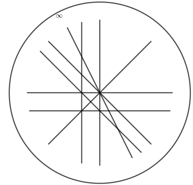
(A) The arrangement $\mathcal{A}$.

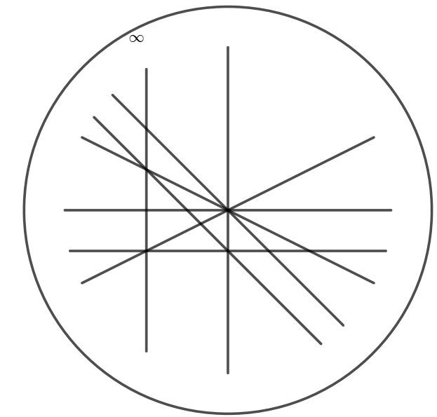
(B) The arrangement $\mathcal{B}$.

Figure 3.1. Two projectivized pictures of the arrangements $\mathcal{A}$ and $\mathcal{B}$.

Corollary 3.4.

If $M$ is a simple matroid of rank not larger than $3$, then $\mathcal{N}_{M}(Y,T)$ has nonnegative coefficients and satisfies

$$\mathcal{N}_{M}(Y^{-1},T^{-1}) =Y^{r(M)}T^{r(M)-1}\mathcal{N}_{M}(Y,T).$$

Moreover, the polynomial $\mathcal{N}_{M}(1,T)$ is real-rooted.

Proof.

This is clear if $r(M)=1$ as we assume that $M$ is a simple matroid. If $M$ has rank $2$, then $M\cong U_{2,n}$, where $n$ is the size of the ground set of $M$. Then,

$$\mathcal{N}_{U_{2,n}}(Y,T) =(1+Y)(1+(n-1)Y)+(1+Y)(n-1+Y)T,$$

which satisfies the three properties.

If $r(M)=3$, then from Proposition 3.2, $\mathcal{N}_{M}(Y,T)$ satisfies

$$\mathcal{N}_{M}(Y^{-1},T^{-1}) =Y^{-3}T^{-2}\mathcal{N}_{M}(Y,T).$$

The nonnegativity of the coefficients follows if $2s-n+c\geqslant 0$. Since every element of the ground set is contained in some rank $2$ flat, it follows that $2s-n\geqslant 0$. Thus, $\mathcal{N}_{M}(Y,T)$ has nonnegative coefficients. The discriminant of $\mathcal{N}_{M}(Y,T)$ as a polynomial in $T$ is

$$\left((c+n)^{2}(1-Y)^{2}-4s(1-(c+1)Y+Y^{2})\right)(1+Y)^{4},$$

which is positive at $Y=1$. ∎

Lemma 3.5.

For all matroids $M$ with rank $3$,

$$(1+T)^{2}<\dfrac{\mathcal{N}_{M}(1,T)}{\pi_{M}(1)}<E_{3}^{\mathsf{B}}(T)=1+6T+T^{2}.$$

Proof.

Without loss of generality, $M$ is a simple matroid. By Proposition 3.2,

(3.1) $$\dfrac{\mathcal{N}_{M}(1,T)}{\pi_{M}(1)} =1+\left(2+\dfrac{4(c-1)}{s-(c-1)}\right)T+T^{2},$$

where $c=|\mathcal{L}_{2}(M)|$ and $s=\sum_{X\in\mathcal{L}_{2}(M)}|X|$. Since $s\geqslant 2c$,

$$0 <\dfrac{4(c-1)}{s-(c-1)}<4.\qed$$

We note that equation (3.1) together with Theorem 1.2 proves Corollary 1.3.

4. Oriented matroids

Central to the proof of Theorem 1.2 is the face lattice of an oriented matroid $M=(E,\mathcal{C})$. Recall from Section 2.2 that $\mathcal{C}$ is the set of covectors, $\mathcal{F}(\mathcal{C})$ the face lattice, $\mathcal{T}(\mathcal{C})$ the set of topes, and $\mathrm{z}:\mathcal{C}\rightarrow 2^{E}$ the zero map.

For a poset $P$, let $\widehat{\Delta}(P)$, resp. $\widehat{\Delta}_{k}(P)$, be the set of nonempty flags, resp. flags of length $k$, ending at a maximal element of $P$.

A key result that will be applied multiple times for our proof of Theorem 1.2 is the Las Vergnas–Zaslavsky Theorem.

Theorem 4.1 ([4, Theorem 4.6.1]).

Let $M=(E,\mathcal{C})$ be an oriented matroid. Then

$$|\mathcal{T}(\mathcal{C})|=\pi_{M}(1).$$

Lemma 4.2.

Let $M=(E,\mathcal{C})$ be an oriented matroid of rank $r$. Then for all $k\in[r]$,

$$\left|\widehat{\Delta}_{k}(\overline{\mathcal{F}}(\mathcal{C}))\right| =\sum_{F\in\Delta_{k-1}(\overline{\mathcal{L}}(M))}\pi_{F}(1).$$

Proof.

We prove this by induction on $k$, where the case $k=1$ is Theorem 4.1, so we assume it holds for some $k\geqslant 1$.

For $X\in\overline{\mathcal{L}}(M)$, the matroids $M|X$ and $M/X$ are orientable. The set of covectors of $M/X$ is $\mathcal{C}/X:=\left\{C|_{E\setminus X}:C\in\mathcal{C},X\subseteq\mathrm{z}(C)\right\}$, and the set of covectors of $M|X$ is $\mathcal{C}|X:=\left\{C|_{X}:C\in\mathcal{C}\right\}$. Then by induction

(4.1) $$\begin{split}\sum_{F\in\Delta_{k}(\overline{\mathcal{L}}(M))}\pi_{F}(1)&=\sum_{X\in\overline{\mathcal{L}}(M)}~{}\sum_{F^{\prime}\in\Delta_{k-1}(\overline{\mathcal{L}}(M|X))}\pi_{M/X}(1)\pi_{F^{\prime}}(1)\\ &=\sum_{X\in\overline{\mathcal{L}}(M)}\pi_{M/X}(1)\left|\widehat{\Delta}_{k}(\overline{\mathcal{F}}(\mathcal{C}|X))\right|\\ &=\sum_{X\in\overline{\mathcal{L}}(M)}\left|\mathcal{T}(\mathcal{C}/X)\right|\left|\widehat{\Delta}_{k}(\overline{\mathcal{F}}(\mathcal{C}|X))\right|.\end{split}$$

The last equation in (4.1) follows from Theorem 4.1.

Fix $X\in\overline{\mathcal{F}}(M)$. The set of topes $\mathcal{T}(\mathcal{C}/X)$ is canonically in bijection with the set $\{C\in\mathcal{C}:\mathrm{z}(C)=X\}$. Hence, the set $\mathcal{T}(\mathcal{C}/X)\times\widehat{\Delta}_{k}(\overline{\mathcal{F}}(\mathcal{C}|X))$ determines a flag in $\widehat{\Delta}_{k+1}(\overline{\mathcal{F}}(\mathcal{C}))$ beginning with a face whose zero set is $X$. More precisely, for $C\in\mathcal{T}(\mathcal{C}/X)$ and $F=(C_{1}<\cdots<C_{k})\in\widehat{\Delta}_{k}(\overline{\mathcal{F}}(\mathcal{C}|X))$, we define a flag $(C^{\prime}<C_{1}^{\prime}<\cdots<C_{k}^{\prime})\in\widehat{\Delta}_{k+1}(\overline{\mathcal{F}}(\mathcal{C}))$ such that

$$C_{e}^{\prime} =\begin{cases}C_{e}&e\in E\setminus X,\\ 0&e\in X,\end{cases}$$

and for $i\in[k]$,

$$(C_{i}^{\prime})_{e} =\begin{cases}C_{e}&e\in E\setminus X,\\ (C_{i})_{e}&e\in X.\end{cases}$$

Lastly, the number of flags in $\widehat{\Delta}_{k+1}(\overline{\mathcal{F}}(\mathcal{C}))$ beginning with a face whose zero set is $X\in\overline{\mathcal{L}}(M)$ is $\left|\mathcal{T}(\mathcal{C}/X)\right|\left|\widehat{\Delta}_{k}(\overline{\mathcal{F}}(\mathcal{C}|X))\right|$. Hence, by (4.1), the lemma holds. ∎

For a finite simplicial complex $\Sigma$, we write $f(\Sigma):=(f_{0},\dots,f_{d})\in\mathbb{N}_{0}^{d+1}$ for the $f$-vector of $\Sigma$, where $f_{k}$ is the number of $k$-subsets in $\Sigma$—equivalently, the number of $(k-1)$-dimensional faces. Let $f(\Sigma;T)=\sum_{k=0}^{d}f_{k}T^{k}$ be the $f$-polynomial of $\Sigma$, and let $h(\Sigma;T):=(1-T)^{d}f(\Sigma;T/(1-T))$, which is the $h$-polynomial associated to $\Sigma$. The coefficients of $h(\Sigma;T)$ yield the $h$-vector $h(\Sigma)$ of $\Sigma$.

For a tope $\tau\in\mathcal{T}(\mathcal{C})$, we define a simplicial complex $\Sigma(\tau):=\Delta((\hat{0}_{\mathcal{C}},\tau))$, which is the set of flags in the open interval $(\hat{0}_{\mathcal{C}},\tau)$ in $\mathcal{F}(\mathcal{C})$ ordered by refinement. We write $\Sigma_{k}(\tau)$ for the flags of $\Sigma(\tau)$ with length $k$. If $M$ is realizable over $\mathbb{R}$, then $\Sigma(\tau)$ is the barycentric subdivision of the boundary of the chamber determined by $\tau$.

Proposition 4.3.

Let $M=(E,\mathcal{C})$ be an oriented matroid of rank $r$. Then

$$\mathcal{N}_{M}(1,T) =\sum_{\tau\in\mathcal{T}(\mathcal{C})}h(\Sigma(\tau);T).$$

Proof.

The flags in $\widehat{\Delta}(\overline{\mathcal{F}}(\mathcal{C}))$ are partitioned into subsets $\widehat{\Delta}((\hat{0}_{\mathcal{C}},\tau])$ for $\tau\in\mathcal{T}(\mathcal{C})$, and the latter are in bijection with the flags in $\Sigma(\tau)$. Thus, for each $k\in[r-1]_{0}$,

$$\left|\widehat{\Delta}_{k+1}(\overline{\mathcal{F}}(\mathcal{C}))\right| =\sum_{\tau\in\mathcal{T}(\mathcal{C})}\left|\Sigma_{k}(\tau)\right|.$$

Applying Lemma 4.2, we have

$$\sum_{\tau\in\mathcal{T}(\mathcal{C})}h(\Sigma(\tau);T) =\sum_{k=0}^{r-1}\sum_{\tau\in\mathcal{T}(\mathcal{C})}\left|\Sigma_{k}(\tau)\right|T^{k}(1-T)^{r-k-1}$$

$$=\sum_{k=0}^{r-1}~{}\sum_{F\in\Delta_{k}(\overline{\mathcal{L}}(M))}\pi_{F}(1)T^{k}(1-T)^{r-k-1}=\mathcal{N}_{M}(1,T).\qed$$

In order to prove the lower bound in Theorem 1.2, we work with the cd-index of an (Eulerian) poset. Details can be found in [23, Ch. 3.17].

Let $P$ be a graded poset of rank $n$ with rank function $r:P\rightarrow[n]_{0}$. For $S\subseteq[n]_{0}$, let $P_{S}=\{x\in P~{}|~{}r(x)\in S\}$. Set $\alpha_{P}(S)$ to be the number of maximal flags in $P_{S}$, and let

$$\beta_{P}(S)=\sum_{U\subseteq S}(-1)^{|S\setminus U|}\alpha_{P}(U).$$

Let $a$ and $b$ be two noncommuting variables. For a subset $S\subseteq\left[n\right]_{0}$ we define a monomial $u_{S}$ by setting $u_{S}=e_{0}e_{1}\dots e_{n}$, where

$$e_{i}=\begin{cases}a,&\mbox{if }i\not\in S,\\ b,&\mbox{if }i\in S.\end{cases}$$

Using these monomials we can define the $ab$-index $\Psi_{P}(a,b)$ of the graded poset $P$ which is the noncommutative polynomial

$$\Psi_{P}(a,b)=\sum_{S\subseteq\left[n\right]_{0}}\beta_{P}(S)u_{S}.$$

If $P$ is an Eulerian poset, that is every interval in $P$ has an equal number of elements of even and odd rank, there exists a polynomial $\Phi_{P}(c,d)$ in the noncommuting variables $c,d$ such that

$$\Psi_{P}(a,b)=\Phi_{P}(a+b,ab+ba).$$

The polynomial $\Phi_{P}(c,d)$ is called the $cd$-index of the Eulerian poset $P$. For an overview about the $cd$-index see [3].

If $M=(E,\mathcal{C})$ is an oriented matroid of rank $r$, then for $\tau\in\mathcal{T}(\mathcal{C})$ and $k\in[r-1]$,

(4.2) $$h_{k}(\Sigma(\tau))=\sum_{\begin{subarray}{c}S\subseteq[r-1]\\ |S|=k\end{subarray}}\beta_{[\hat{0}_{\mathcal{C}},\tau]}(S).$$

Therefore, since $[\hat{0}_{\mathcal{C}},\tau]$ is Eulerian [4, Cor. 4.3.8], we have

(4.3) $$h(\Sigma(\tau);T)=\Psi_{[\hat{0}_{\mathcal{C}},\tau]}(1,T)=\Phi_{[\hat{0}_{\mathcal{C}},\tau]}(1+T,2T),$$

so the $h$-polynomial can be viewed as a coarsening of the cd-index.

Proposition 4.4.

Let $M=(E,\mathcal{C})$ be an oriented matroid of rank $r$. Then for all $\tau\in\mathcal{T}(\mathcal{C})$,

$$E_{r}^{\mathsf{A}}(T) \leqslant h(\Sigma(\tau);T),$$

and equality holds if and only if $\tau$ is a simplicial tope.

Proof.

A lattice $P$ of rank $r$ is Gorenstein* if it is Cohen–Macaulay and Eulerian. Ehrenborg and Karu [10, Cor. 1.3] proved that such a lattice $P$ satisfies

(4.4) $$\Phi_{B_{r}}(c,d)\leq\Phi_{P}(c,d),$$

where $B_{r}$ is the Boolean lattice of rank $r$. If $\tau\in\mathcal{T}(\mathcal{C})$, then the interval $[\hat{0}_{\mathcal{C}},\tau]$ is both Cohen–Macaulay and Eulerian as shown in [4, Cor. 4.3.7 & 4.3.8]. Thus, using (4.3) we obtain, by substituting $c=1+T$ and $d=2T$ in (4.4), $\Phi_{B_{r}}(1+T,2T)\leq h(\Sigma(\tau);T)$. The claimed inequality thus follows from $\Phi_{B_{r}}(1+T,2T)=E_{r}^{\mathsf{A}}(T)$ as this is the $h$-polynomial of the barycentric subdivision of the $r$-dimensional simplex.

If $\tau$ is a simplicial tope, then $[\hat{0}_{\mathcal{C}},\tau]$ is a Boolean lattice by definition and, thus, $E_{r}^{\mathsf{A}}(T)=h(\Sigma(\tau);T)$. On the other hand, suppose we have $E_{r}^{\mathsf{A}}(T)=h(\Sigma(\tau);T)$ for the tope $\tau\in\mathcal{T}(\mathcal{C})$. This implies

$$h_{1}(\Sigma(\tau))=2^{r}-r-1.$$

By definition we have

$$h_{1}(\Sigma(\tau)) =\sum_{i=1}^{r-1}\left(\alpha_{[\hat{0}_{\mathcal{C}},\tau]}(\{i\})-1\right)=\sum_{i=1}^{r-1}\alpha_{[\hat{0}_{\mathcal{C}},\tau]}(\{i\})-r+1.$$

By [4, Exercise 4.4 (b)] we have $\alpha_{[\hat{0}_{\mathcal{C}},\tau]}(\{i\})\geq\binom{r}{i}$. Altogether this yields

$$\sum_{i=1}^{r-1}\binom{r}{i}=2^{r}-2=\sum_{i=1}^{r-1}\alpha_{[\hat{0}_{\mathcal{C}},\tau]}(\{i\})\geq\sum_{i=1}^{r-1}\binom{r}{i}.$$

Thus we obtain $\alpha_{[\hat{0}_{\mathcal{C}},\tau]}(\{r-1\})=r$ which by [4, Exercise 4.4 (c)] implies that the tope $\tau$ is simplicial. ∎

Proof of Theorem 1.2.

The proof of the first statement follows from Theorem 4.1 and Propositions 4.3 and 4.4. Since $\beta_{[\hat{0}_{\mathcal{C}},\tau]}(S)=\beta_{[\hat{0}_{\mathcal{C}},\tau]}([r-1]\setminus S)$ by [23, Corollary 3.16.6], it follows from Equation (4.2) that $h_{k}(\Sigma(\tau))=h_{r-k-1}(\Sigma(\tau))$. Hence, the second statement follows by Proposition 4.3. ∎

4.1. Examples

We compute $\mathcal{N}_{M}(1,T)$ for some oriented matroids $M$.

4.1.1. A uniform matroid with rank $3$

Consider the matroid $M=U_{3,4}$. One set of covectors is defined by the real arrangement given by $xyz(x+y+z)0$. There are $14=2^{4}-2$ topes since $(+++-)$ and $(---+)$ are not topes. For instance, the inequality system given by $x>0,y>0,z>0$ and $x+y+z<0$ is infeasible. The topes with an even number of $+$ symbols correspond to triangles, and the topes with an odd number of $+$ symbols correspond to squares. Therefore, there are $8$ triangles and $6$ squares, so by Proposition 4.3,

$$\mathcal{N}_{M}(1,T) =8(1+4T+T^{2})+6(1+6T+T^{2})=14+68T+14T^{2}.$$

By Proposition 3.2, the coarse numerator for $M$ is given by

$$\mathcal{N}_{M}(Y,T) =1+4Y+6Y^{2}+3Y^{3}+(8+26Y+26Y^{2}+8Y^{3})T$$

$$\qquad+(3+6Y+4Y^{2}+Y^{3})T^{2}.$$

4.1.2. A uniform matroid with rank $4$

Three uniform matroids, which are not isomorphic to the matroids underlying Coxeter arrangements, in [18] had the seemingly rare property that $\mathcal{N}_{M}(1,T)/\pi_{M}(1)\in\mathbb{Z}[T]$. These are the uniform matroids $U_{r,n}$ for

$$(r,n)\in\{(4,5),(4,7),(4,8)\},$$

and we consider $(r,n)=(4,7)$. From Proposition 4.3, this integrality condition is equivalent to the integrality of the average of the $h$-vectors. To do this computation, we used the hyperplane arrangement package [17] of polymake version 4.4 [15].

The matroid $U_{4,7}$ can be realized as a hyperplane arrangement in $\mathbb{R}^{4}$, whose hyperplanes are given by

$$x_{1}x_{2}x_{3}x_{4}(x_{1}+x_{2}+x_{3}+x_{4})(x_{1}+2x_{2}+3x_{3}+4x_{4})(x_{1}+3x_{2}+2x_{2}+5x_{4})=0.$$

There are five different polytopes corresponding to chambers of this arrangement, and they can be seen in Figure 4.1. The chambers are $4$-dimensional cones over these polytopes.

(A)

(B)

(C)

(D)

(E)

Figure 4.1. The five different polytopes arising as chambers in the $U_{4,7}$ arrangement.

There are a total of 84 chambers; 22 are simplices, 22 are triangular prisms, 30 are the polytopes seen in Figure 1(C), six are the polytopes seen in Figure 1(D), and four are truncated simplices as seen in Figure 1(E). The $h$-vectors of the barycentric subdivisions are palindromic, and the first values different from $1$ are $11$, $17$, $23$, $29$, and $29$ respectively. Thus,

$$\mathcal{N}_{U_{4,7}}(1,T) =22(1+11T+11T^{2}+T^{3})+22(1+17T+17T^{2}+T^{3})$$

$$\qquad+30(1+23T+23T^{2}+T^{3})+(4+6)(1+29T+29T^{2}+T^{3}).$$

This has the nice coincidence that

$$\mathcal{N}_{U_{4,7}}(1,T) =84(1+19T+19T^{2}+T^{3}).$$

Curiously, $(1,19,19,1)$ is the $h$-vector of the barycentric subdivision of the pyramid over a pentagon.

4.2. Rank $4$ oriented matroids

In this section, we prove that $\mathcal{N}_{M}(1,T)$, for an oriented matroid $M=(E,\mathcal{C})$ of rank $4$, is bounded above coefficient-wise by $\pi_{M}(1)E_{r}^{\mathsf{B}}(T)$. The next lemma determines the coefficients of $\mathcal{N}_{M}(1,T)$ in terms of the face lattice of $M$. To simplify notation, we define

$$\mathfrak{f}_{k}(\mathcal{C}):=\left|\widehat{\Delta}_{k+1}\left(\overline{\mathcal{F}}(\mathcal{C})\right)\right|=\left|\left\{F\in\Delta_{k+1}\left(\overline{\mathcal{F}}(\mathcal{C})\right):F\text{ ends at a tope}\right\}\right|.$$

For $f(T)=\sum_{k\geqslant 0}a_{k}T^{k}$, let $f(T)[T^{k}]=a_{k}$.

Lemma 4.5.

Let $M=(E,\mathcal{C})$ be an oriented matroid of rank $r$. For $\ell\in[r-1]_{0}$,

$$\mathcal{N}_{M}(1,T)[T^{\ell}] =\sum_{k=0}^{\ell}(-1)^{\ell-k}\mathfrak{f}_{k}(\mathcal{C})\binom{r-k-1}{\ell-k}.$$

Proof.

Let $\tau\in\mathcal{T}(\mathcal{C})$ and let $f(\Sigma(\tau);T)$ be the $f$-polynomial. The coefficient of $T^{\ell}$ in the $h$-polynomial of $\Sigma(\tau)$ is

$$h_{\ell}(\Sigma(\tau))=\sum_{k=0}^{\ell}(-1)^{\ell-k}f_{k}(\Sigma(\tau))\binom{r-k-1}{\ell-k}.$$

By Proposition 4.3,

$$\mathcal{N}_{M}(1,T)[T^{\ell}] =\sum_{\tau\in\mathcal{T}(\mathcal{C})}\sum_{k=0}^{\ell}(-1)^{\ell-k}f_{k}(\Sigma(\tau))\binom{r-k-1}{\ell-k}$$

$$=\sum_{k=0}^{\ell}(-1)^{\ell-k}\mathfrak{f}_{k}(\mathcal{C})\binom{r-k-1}{\ell-k}.\qed$$

Proposition 4.6.

If $M$ is an orientable matroid of rank $r\geqslant 3$, then

$$\mathcal{N}_{M}(1,T)[T]<\pi_{M}(1)E_{r}^{\mathsf{B}}(T)[T].$$

If $M$ is of rank $4$, then $\mathcal{N}_{M}(1,T)<\pi_{M}(1)E_{4}^{\mathsf{B}}(T)$.

Proof.

From Theorem 1.2, $\mathcal{N}_{M}(1,T)$ has degree $r-1$ and is palindromic. Therefore it suffices to just prove the inequality between the linear coefficients.

Suppose $\mathcal{C}$ is a set of covectors such that $M=(E,\mathcal{C})$ is an oriented matroid. The number $\mathfrak{f}_{1}(\mathcal{C})$ counts the flags of length two in $\overline{\mathcal{F}}(\mathcal{C})$ which end at a tope, and $\mathfrak{f}_{0}(\mathcal{C})=|\mathcal{T}(\mathcal{C})|$. Using Proposition 4.6.9 of [4], we have the following inequality:

(4.5) $$\mathfrak{f}_{1}(\mathcal{C}) <\sum_{j=0}^{r-2}2^{r-1-j}\binom{r-1}{j}|\mathcal{T}(\mathcal{C})|.$$

Using [21, Sec. 13.1], one can express the terms of $E_{r}^{\mathsf{B}}(T)$ in terms of alternating sums. The linear term is, thus, $3^{r-1}-r$.

$$\mathcal{N}_{M}(1,T)[T] =\mathfrak{f}_{1}(\mathcal{C})-(r-1)\mathfrak{f}_{0}(\mathcal{C}) (\text{Lemma~{}\ref{lem:N-terms}})$$

$$<\left(\sum_{j=0}^{r-2}2^{r-1-j}\binom{r-1}{j}|\mathcal{T}(\mathcal{C})|\right)-(r-1)|\mathcal{T}(\mathcal{C})| (\text{Eq.~{}\ref{eqn:Varchenko-bound}})$$

$$=(3^{r-1}-1)|\mathcal{T}(\mathcal{C})|-(r-1)|\mathcal{T}(\mathcal{C})|$$

$$=\pi_{M}(1)E_{r}^{\mathsf{B}}[T].$$

The penultimate equality is seen by counting, in two different ways, the number of ways to color $r-1$ balls with three colors. ∎

5. Extremal families

In this section, we prove Theorem 1.5 in two parts by constructing infinite families of matroids whose normalized coarse flag polynomial is arbitrarily close to the bounds given in Conjecture 1.4. The upper bound is witnessed by the family of uniform matroids, and the lower bound is witnessed by the family of finite projective geometries. See Section 2.1 for definitions.

In what follows, we compute limits of univariate polynomials of a fixed degree. Identifying degree $d$ polynomials $a_{0}+a_{1}T+\cdots+a_{d}T^{d}$ with the points $(a_{0},\dots,a_{d})\in\mathbb{R}^{d+1}$, the limit is determined using the Euclidean norm in $\mathbb{R}^{d+1}$.

5.1. The upper bound

The next lemma relates the type $\mathsf{B}$ Eulerian polynomial $E_{r}^{\mathsf{B}}$ with the type $\mathsf{A}$ Eulerian polynomial $E_{r}^{\mathsf{A}}$, which may be of independent interest.

Lemma 5.1.

For $r\in\mathbb{N}$,

(5.1) $$E_{r}^{\mathsf{B}}(T) =(1-T)^{r-1}+\sum_{k=1}^{r-1}2^{k}\binom{r-1}{k}T(1-T)^{r-k-1}E_{k}^{\mathsf{A}}(T).$$

Proof.

Let $P_{r}(T)$ denote the polynomial on the right side in (5.1). It is clear that $P_{1}(T)=E^{\mathsf{B}}_{1}(T)=1$, so we assume $r\geqslant 2$. Recall two recurrence relations concerning the two Eulerian polynomials [21, Thms. 1.4 & 13.2]; namely,

$$E_{r+1}^{\mathsf{A}} =(1+rT)E_{r}^{\mathsf{A}}+T(1-T)\dfrac{\mathrm{d}E_{r}^{\mathsf{A}}}{\mathrm{d}T},$$

$$E_{r+1}^{\mathsf{B}} =(1+(2r-1)T)E_{r}^{\mathsf{B}}+2T(1-T)\dfrac{\mathrm{d}E_{r}^{\mathsf{B}}}{\mathrm{d}T}.$$

We will prove that $P_{r}(T)$ satisfies the type $\mathsf{B}$ recurrence relation, and thus the lemma will follow.

Applying the type $\mathsf{A}$ recurrence relation on Eulerian polynomials, we have

$$2T(1-T)\dfrac{\mathrm{d}P_{r}}{\mathrm{d}T} =2T(1-r)(1-T)^{r-1}$$

$$\qquad+\sum_{k=1}^{r-1}2^{k+1}\binom{r-1}{k}T(1-T)^{r-k-1}\left(E_{k+1}^{\mathsf{A}}-rTE_{k}^{\mathsf{A}}\right).$$

Lastly, we have

$$(1+(2r-1)T)P_{r}(T)+2T(1-T)\dfrac{\mathrm{d}P_{r}}{\mathrm{d}T}(T)$$

$$=(1-T)^{r}+2T(1-T)^{r-1}+\sum_{k=1}^{r-1}2^{k+1}\binom{r-1}{k}T(1-T)^{r-k-1}E_{k+1}^{\mathsf{A}}$$

$$\qquad+\sum_{k=1}^{r-1}2^{k}\binom{r-1}{k}T(1-T)^{r-k}E_{k}^{\mathsf{A}}$$

$$=(1-T)^{r}+2T(1-T)^{r-1}+2^{r}TE_{r}^{\mathsf{A}}+2(r-1)T(1-T)^{r-1}$$

$$\qquad+\sum_{k=2}^{r-1}2^{k}\binom{r-1}{k-1}T(1-T)^{r-k}E_{k}^{\mathsf{A}}+\sum_{k=2}^{r-1}2^{k}\binom{r-1}{k}T(1-T)^{r-k}E_{k}^{\mathsf{A}}$$

$$=(1-T)^{r}+\sum_{k=1}^{r}2^{k}\binom{r}{k}T(1-T)^{r-k}E_{k}^{\mathsf{A}}=P_{r+1}(T).\qed$$

Proposition 5.2.

For $r\in\mathbb{N}$,

$$\lim_{m\rightarrow\infty}\dfrac{\mathcal{N}_{U_{r,m}}(1,T)}{\pi_{U_{r,m}}(1)} =E^{\mathsf{B}}_{r}(T).$$

Proof.

From [18, Proposition 6.9],

$$\dfrac{\mathcal{N}_{U_{r,m}}(1,T)}{\pi_{U_{r,m}}(1)} =(1-T)^{r-1}+\dfrac{\sum_{\ell=1}^{r-1}\sum_{k=0}^{r-\ell-1}\binom{m}{\ell}\binom{m-\ell-1}{k}2^{\ell}T(1-T)^{r-\ell-1}E_{\ell}^{\mathsf{A}}}{\sum_{k=0}^{r-1}\binom{m-1}{k}}$$

$$=(1-T)^{r-1}+\sum_{\ell=1}^{r-1}2^{\ell}T(1-T)^{r-\ell-1}E_{\ell}^{\mathsf{A}}\left(\dfrac{\binom{m}{\ell}\sum_{k=0}^{r-\ell-1}\binom{m-\ell-1}{k}}{\sum_{k=0}^{r-1}\binom{m-1}{k}}\right).$$

For $\ell\in[r-1]$, it follows that

$$\lim_{m\rightarrow\infty}\dfrac{\binom{m}{\ell}\sum_{k=0}^{r-\ell-1}\binom{m-\ell-1}{k}}{\sum_{k=0}^{r-1}\binom{m-1}{k}} =\binom{r-1}{\ell}.$$

Therefore,

(5.2) $$\lim_{m\rightarrow\infty}\dfrac{\mathcal{N}_{U_{r,m}}(1,T)}{\pi_{U_{r,m}}(1)} =(1-T)^{r-1}+\sum_{\ell=1}^{r-1}2^{\ell}\binom{r-1}{\ell}T(1-T)^{r-\ell-1}E_{\ell}^{\mathsf{A}}.$$

By Lemma 5.1, the right side of (5.2) is $E^{\mathsf{B}}_{r}(T)$. ∎

5.2. The lower bound

For an indeterminate $X$, a nonnegative integer $r$, and $0\leqslant k\leqslant r$, we set

$$\binom{r}{k}_{X}=\dfrac{(1-X^{r})(1-X^{r-1})\cdots(1-X^{r-k+1})}{(1-X)(1-X^{2})\cdots(1-X^{k})}\in\mathbb{Z}[X].$$

For $I\subseteq[r-1]$, where $I=\{i_{1}<\cdots<i_{k}\}$, we set $i_{0}=0$, $i_{k+1}=r$, and

$$\binom{r}{I}_{X}=\prod_{m=1}^{|I|}\binom{i_{m+1}}{i_{m}}_{X}=\binom{r}{i_{k}}_{X}\binom{i_{k}}{i_{k-1}}_{X}\cdots\binom{i_{2}}{i_{1}}_{X}.$$

The number of $k$-dimensional subspaces of $\mathbb{F}_{q}^{r}$ is equal to $\binom{r}{k}_{q}$. For $I\subseteq[r-1]$, the number of flags $0=V_{0}\subset V_{1}\subset\cdots\subset V_{k}\subset V_{k+1}=\mathbb{F}_{q}^{r}$ with $I=\{\dim(V_{j})~{}|~{}j\in[k]\}$ is equal to $\binom{r}{I}_{q}$. Throughout this subsection, we will assume that when $I\subseteq[r-1]$, then $I=\{i_{1},\dots,i_{k}\}$, where $i_{j}<i_{j+1}$ for $j\in[k-1]$. We define the polynomial

$$\gamma_{I}(X,Y) =\prod_{\ell=0}^{|I|}~{}\prod_{m=0}^{i_{\ell+1}-i_{\ell}-1}(1+X^{m}Y).$$

Let $M=PG(r-1,q)$ be the matroid determined by the projective geometry of dimension $r$ and order $q$. Thus, the lattice of flats of $M$ is isomorphic to the subspace lattice of the finite vector space $\mathbb{F}_{q}^{r}$. The Poincaré polynomial of $M$ is $\pi_{M}(Y)=\gamma_{\varnothing}(q,Y)$ since the Möbius function values of a flat of rank $k$ in $\mathcal{L}(M)$ is $(-1)^{k}q^{\binom{k}{2}}$.

Lemma 5.3.

For $r\in\mathbb{N}$ and a prime power $q$,

$$\mathcal{N}_{PG(r-1,q)}(Y,T)=\sum_{I\subseteq[r-1]}\binom{n}{I}_{q}\gamma_{I}(q,Y)T^{|I|}(1-T)^{r-1-|I|}.$$

Proof.

Let $M=PG(r-1,q)$. It follows that $\Delta(\overline{\mathcal{L}}(M))$ is in bijection with the set of flags in $\mathbb{F}_{q}^{r}$ with proper nontrivial subspaces. Let $I\subseteq[r-1]$, and suppose $F$ and $F^{\prime}$ are flags in $\mathbb{F}_{q}^{r}$ of length $|I|$ containing proper nontrivial subspaces, whose dimensions are given by $I$. It follows that $\pi_{F}(Y)=\pi_{F^{\prime}}(Y)$ since the intervals in $\Delta(\overline{\mathcal{L}}(M))$ determined by $F$ and $F^{\prime}$ are isomorphic. In particular, $\pi_{F}(Y)$ is determined by $I$, the set of (proper nontrivial) subspace dimensions. Furthermore, each interval is isomorphic to the lattice of flats of some projective geometry of order $q$ with smaller dimension. Therefore, $\pi_{F}(Y)=\gamma_{I}(q,Y)$.

Since the number of flags $F$ with a given set of subspace dimensions $I\subseteq[r-1]$ is $\binom{r}{I}_{q}$, it follows that

$$\mathcal{N}_{M}(Y,T) =\sum_{F\in\Delta(\overline{\mathcal{L}}(M))}\pi_{F}(Y)T^{|F|}(1-T)^{r-1-|F|}$$

$$=\sum_{I\subseteq[r-1]}\binom{r}{I}_{q}\gamma_{I}(q,Y)T^{|I|}(1-T)^{r-1-|I|}.\qed$$

Proposition 5.4.

Let $r\in\mathbb{N}$ and

$$\lim_{q\rightarrow\infty}\dfrac{\mathcal{N}_{PG(r-1,q)}(1,T)}{\pi_{PG(r-1,q)}(1)}=(1+T)^{r-1},$$

where $q$ is assumed to be a prime power.

Proof.

Let $X$ be an indeterminate, and note that for $I\subseteq[r-1]$,

$$\lim_{X\rightarrow\infty}\dfrac{\binom{n}{I}_{X}\gamma_{I}(X,1)}{\gamma_{\varnothing}(X,1)}=2^{|I|}.$$

Set $M=PG(r-1,q)$, and since $\pi_{M}(Y)=\varphi_{\varnothing}(q,Y)$, by Lemma 5.3,

$$\lim_{q\rightarrow\infty}\dfrac{\mathcal{N}_{M}(1,T)}{\pi_{M}(1)} =\sum_{I\subseteq[r-1]}2^{|I|}T^{|I|}(1-T)^{r-1-|I|}$$

$$=\sum_{k=0}^{r-1}\binom{r-1}{k}(1-T)^{r-1-k}(2T)^{k}$$

$$=(1+T)^{r-1}.\qed$$

5.3. Proof of Theorem 1.5

The first part follows from Propositions 5.2 and 5.4, and the second part follows from Propositions 3.2 and 4.6. $\square$

References

• [1] F. Ardila and M. Sanchez. Valuations and the Hopf Monoid of Generalized Permutahedra. Int. Math. Res. Not. IMRN, 2022.
• [2] M. Barakat, R. Behrends, C. Jefferson, L. Kühne, and M. Leuner. On the generation of rank 3 simple matroids with an application to Terao’s freeness conjecture. SIAM J. Discrete Math., 35(2):1201–1223, 2021.
• [3] M. M. Bayer. The $cd$-index: a survey. In Polytopes and discrete geometry, volume 764 of Contemp. Math., pages 1–19. Amer. Math. Soc., Providence, RI, 2021.
• [4] A. Björner, M. Las Vergnas, B. Sturmfels, N. White, and G. M. Ziegler. Oriented matroids, volume 46 of Encyclopedia of Mathematics and its Applications. Cambridge University Press, Cambridge, second edition, 1999.
• [5] F. Brenti and V. Welker. $f$-vectors of barycentric subdivisions. Math. Z., 259(4):849–865, 2008.
• [6] N. Budur, M. Saito, and S. Yuzvinsky. On the local zeta functions and the $b$-functions of certain hyperplane arrangements. J. Lond. Math. Soc. (2), 84(3):631–648, 2011. With an appendix by Willem Veys.
• [7] J. Csima and E. T. Sawyer. There exist $6n/13$ ordinary points. Discrete Comput. Geom., 9(2):187–202, 1993.
• [8] M. Cuntz and D. Geis. Combinatorial simpliciality of arrangements of hyperplanes. Beitr. Algebra Geom., 56(2):439–458, 2015.
• [9] H. Derksen and A. Fink. Valuative invariants for polymatroids. Adv. Math., 225(4):1840–1892, 2010.
• [10] R. Ehrenborg and K. Karu. Decomposition theorem for the ${\bf cd}$-index of Gorenstein posets. J. Algebraic Combin., 26(2):225–251, 2007.
• [11] B. Elias, N. Proudfoot, and M. Wakefield. The Kazhdan-Lusztig polynomial of a matroid. Adv. Math., 299:36–70, 2016.
• [12] C. Eur. Divisors on matroids and their volumes. J. Combin. Theory Ser. A, 169:105135, 31, 2020.
• [13] L. Ferroni and B. Schröter. Valuative invariants for large classes of matroids, 2022. arXiv:2208.04893.
• [14] K. Fukuda, A. Tamura, and T. Tokuyama. A theorem on the average number of subfaces in arrangements and oriented matroids. Geom. Dedicata, 47(2):129–142, 1993.
• [15] E. Gawrilow and M. Joswig. polymake: a framework for analyzing convex polytopes. In Polytopes—combinatorics and computation (Oberwolfach, 1997), volume 29 of DMV Sem., pages 43–73. Birkhäuser, Basel, 2000.
• [16] D. Jensen, M. Kutler, and J. Usatine. The motivic zeta functions of a matroid. J. Lond. Math. Soc. (2), 103(2):604–632, 2021.
• [17] L. Kastner and M. Panizzut. Hyperplane arrangements in polymake. In A. M. Bigatti, J. Carette, J. H. Davenport, M. Joswig, and T. de Wolff, editors, Mathematical Software – ICMS 2020, pages 232–240, Cham, 2020. Springer International Publishing.
• [18] J. Maglione and C. Voll. Flag Hilbert–Poincaré series of hyperplane arrangements and their Igusa zeta functions, 2021. arXiv:2103.03640.
• [19] Y. Matsumoto, S. Moriyama, H. Imai, and D. Bremner. Matroid enumeration for incidence geometry. Discrete Comput. Geom., 47(1):17–43, 2012.
• [20] P. Orlik and H. Terao. Arrangements of hyperplanes, volume 300 of Grundlehren der mathematischen Wissenschaften [Fundamental Principles of Mathematical Sciences]. Springer-Verlag, Berlin, 1992.
• [21] T. K. Petersen. Eulerian numbers. Birkhäuser Advanced Texts: Basler Lehrbücher. [Birkhäuser Advanced Texts: Basel Textbooks]. Birkhäuser/Springer, New York, 2015. With a foreword by Richard Stanley.
• [22] T. Rossmann and C. Voll. Groups, graphs, and hypergraphs: average sizes of kernels of generic matrices with support constraints, 2019. arXiv:1908.09589.
• [23] R. P. Stanley. Enumerative combinatorics. Vol. 1, volume 49 of Cambridge Studies in Advanced Mathematics. Cambridge University Press, Cambridge, 1997. With a foreword by Gian-Carlo Rota, Corrected reprint of the 1986 original.
• [24] R. van der Veer. Combinatorial analogs of topological zeta functions. Discrete Math., 342(9):2680–2693, 2019.
• [25] A. N. Varchenko. The numbers of faces of a configuration of hyperplanes. Dokl. Akad. Nauk SSSR, 302(3):527–530, 1988.