Intermediate dimensions of Bedford–McMullen carpets with applications to Lipschitz equivalence

Abstract.

Intermediate dimensions were recently introduced to provide a spectrum of dimensions interpolating between Hausdorff and box-counting dimensions for fractals where these differ. In particular, the self-affine Bedford–McMullen carpets are a natural case for investigation, but until now only very rough bounds for their intermediate dimensions have been found. In this paper, we determine a precise formula for the intermediate dimensions $\dim_{\,\theta}\Lambda$ of any Bedford–McMullen carpet $\Lambda$ for the whole spectrum of $\theta\in[0,1]$, in terms of a certain large deviations rate function. The intermediate dimensions exist and are strictly increasing in $\theta$, and the function $\theta\mapsto\dim_{\,\theta}\Lambda$ exhibits interesting features not witnessed on any previous example, such as having countably many phase transitions, between which it is analytic and strictly concave.

We make an unexpected connection to multifractal analysis by showing that two carpets with non-uniform vertical fibres have equal intermediate dimensions if and only if the Hausdorff multifractal spectra of the uniform Bernoulli measures on the two carpets are equal. Since intermediate dimensions are bi-Lipschitz invariant, this shows that the equality of these multifractal spectra is a necessary condition for two such carpets to be Lipschitz equivalent.

Figure 1. Intermediate dimensions give finer geometric information about the fractal set. Left: a Bedford–McMullen carpet $\Lambda$ in red and the images of $[0,1]^{2}$ under the iterated function system generating $\Lambda$ in gray. Right: certain bounds for the intermediate dimensions $\dim_{\,\theta}\Lambda$ in green and orange, and the true value in blue obtained in this paper.

1. Introduction

In dimension theory, the two most studied notions of dimension are the Hausdorff and box (also called Minkowski) dimension. For a specific set, a central question is whether its Hausdorff and box dimension are distinct or not. Intuitively, a dimension gap occurs when the set is inhomogeneous in space, and thus cannot be covered optimally by using sets of equal diameter. There are many sets in $\mathbb{R}^{d}$ which exhibit this phenomena: for example convergent sequences, elliptical polynomial spirals, attenuated topologists’ sine curves; or dynamically defined attractors such as limit sets of infinite conformal iterated function systems, self-affine carpet-like constructions in the plane and sponges in higher dimensions; or images of sets under certain stochastic processes [9, 13]; or even the connected component of supercritical fractal percolation [8].

A recent line of research has been initiated by Falconer, Fraser and Kempton [19] in order to get a better understanding of the subtle differences between the Hausdorff and box dimensions. The idea is that by introducing a continuum of intermediate dimensions which interpolate between these two notions of dimension, one can obtain more nuanced information about the geometry of the set. This is done by imposing increasing restrictions on the relative sizes of covering sets governed by a parameter $0\leq\theta\leq 1$. The Hausdorff and box dimension are the two extreme cases when $\theta=0$ and $1$, respectively. Throughout, the diameter of a set $F$ is denoted by $|F|$, its Hausdorff dimension by $\dim_{\mathrm{H}}F$ and its lower and upper box dimensions by $\underline{\dim}_{\mathrm{B}}F$ and $\overline{\dim}_{\mathrm{B}}F$. A finite or countable collection of sets $\{U_{i}\}$ is a cover of $F$ if $F\subseteq\bigcup_{i}U_{i}.$

Definition 1.1.

For $0\leq\theta\leq 1$, the lower $\theta$-intermediate dimension of a bounded set $F\subset\mathbb{R}^{d}$ is given by

$$\underline{\dim}_{\,\theta}F=\inf\{s\geq 0:\,\text{for all }\varepsilon>0\text{ and all }\delta_{0}>0,\text{ there exists }0<\delta\leq\delta_{0}\\ \text{ and a cover }\{U_{i}\}\text{ of }F\text{ such that }\delta^{1/\theta}\leq|U_{i}|\leq\delta\text{ and }{\textstyle\sum}|U_{i}|^{s}\leq\varepsilon\},$$

while its upper $\theta$-intermediate dimension is

$$\overline{\dim}_{\,\theta}F=\inf\{s\geq 0:\,\text{for all }\varepsilon>0\text{ there exists }\delta_{0}>0\text{ such that for all }0<\delta\leq\delta_{0},\\ \text{ there is a cover }\{U_{i}\}\text{ of }F\text{ such that }\delta^{1/\theta}\leq|U_{i}|\leq\delta\text{ and }{\textstyle\sum}|U_{i}|^{s}\leq\varepsilon\}.$$

For a given $\theta$, if the values of $\underline{\dim}_{\,\theta}F$ and $\overline{\dim}_{\,\theta}F$ coincide, then the common value is called the $\theta$-intermediate dimension and is denoted by $\dim_{\,\theta}F$. We refer to the quantity ${\textstyle\sum}|U_{i}|^{s}$ as the $s$-cost of the cover.

With these definitions, $\underline{\dim}_{0}F=\overline{\dim}_{0}F=\dim_{\mathrm{H}}F$, $\underline{\dim}_{1}F=\underline{\dim}_{\mathrm{B}}F$ and $\overline{\dim}_{1}F=\overline{\dim}_{\mathrm{B}}F$, see [16, Chapter 2, Section 3.2]. For the Hausdorff dimension there are no restrictions on the diameters of the covering sets, for the box dimension the diameters of the covering sets must be the same, while for $\dim_{\,\theta}F$ the restriction is to only consider covering sets with diameter in the range $[\delta^{1/\theta},\delta]$. As $\theta\to 0$, the $\theta$-intermediate dimension gives more insight into which scales are used in the optimal cover to reach the Hausdorff dimension. For $\theta<1$, a natural covering strategy to improve on the exponent given by the box dimension is to use covering sets with diameter of the two permissible extremes, in other words either $\delta^{1/\theta}$ or $\delta$. Intuitively, it is more cost efficient in terms of $s$-cost to cover $F$ with sets of diameter $\delta^{1/\theta}$ where $F$ is “sparse” in some appropriate sense and use the larger sets of diameter $\delta$ where $F$ is “dense”.

Most previous examples whose $\theta$-intermediate dimensions are known explicitly [11, 18, 19, 42] share the common feature that the function $\theta\mapsto\dim_{\,\theta}F$ for the range of $\theta$ where $\dim_{\,\theta}F>\dim_{\mathrm{H}}F$ is strictly increasing, concave and analytic, in particular there are no phase transitions. Interestingly, except in [2], the heuristic of using the two extreme scales already leads to the optimal covering strategy. In the proof of [2, Theorem 3.5], Banaji and Fraser use many different scales between $\delta^{1/\theta}$ and $\delta$ to compute the intermediate dimensions of limit sets of infinite conformal iterated function systems (including continued fraction sets), though it is not shown that this is necessary. The standard approach to see whether a covering strategy gives the optimal exponent is to check whether a mass distribution principle [19, Proposition 2.2] applied to a measure constructed from this particular cover gives the matching lower bound.

Intermediate dimensions can also be formulated using capacity theoretic methods [10]. This approach has been used to bound the Hölder regularity of maps that can deform one spiral into another [11], compute the almost-sure value of the intermediate dimension of the image of Borel sets under index-$\alpha$ fractional Brownian motion in terms of dimension profiles [9] and under more general Rosenblatt processes [13].

Qualitative information about $\dim_{\,\theta}F$ can also yield interesting applications. For example, the intermediate dimensions can be used to give information about the Hölder distortion of maps between sets (see [21, Section 17.10] for discussion of the Hölder mapping problem in the context of dimension theory). In [17, Section 2.1 5.] Falconer noted that if $F\subset\mathbb{R}^{d}$ is non-empty and bounded and $f\colon F\to\mathbb{R}^{d}$ is an $\alpha$-Hölder map for some $\alpha\in(0,1]$, meaning that there exists $c>0$ such that $\|f(x)-f(y)\|\leq c\|x-y\|^{\alpha}$ for all $x,y\in F$, then

$$\overline{\dim}_{\,\theta}f(F)\leq\alpha^{-1}\overline{\dim}_{\,\theta}F$$ (1.1)

and $\underline{\dim}_{\,\theta}f(F)\leq\alpha^{-1}\underline{\dim}_{\,\theta}F$ (see [9, Theorem 3.1] and [1, Section 4] for further Hölder distortion estimates). In [2, Example 4.5], Banaji and Fraser showed that the intermediate dimensions can give better information about the Hölder distortion between some continued fraction sets than the Hausdorff or box dimensions.

The intermediate dimensions can also have applications to the orthogonal projections of a set, see [10, Section 6], and images of a set under index-$\alpha$ fractional Brownian motion, see [9, Section 3]. This relies on the intermediate dimensions of the set in question being continuous at $\theta=0$. In [19, Proposition 2.1] it was shown that $\theta\mapsto\underline{\dim}_{\,\theta}F$ and $\theta\mapsto\overline{\dim}_{\,\theta}F$ are continuous for $\theta\in(0,1]$, but there are examples of sets whose intermediate dimensions are discontinuous at $\theta=0$. Banaji introduced a more general family of dimensions, called the $\Phi$-intermediate dimensions, in [1], which can provide more refined geometric information about such sets.

We mention a similar concept of dimension interpolation between the upper box dimension and the (quasi-)Assouad dimension, called the Assouad spectrum, which was initiated in [24, 25]. We refer the reader to the recent surveys [17, 23] for additional references on the topic of dimension interpolation.

An important method for generating fractal sets is via iterated function systems (IFSs); see [16] for general background. In this paper, we consider self-affine sets, which are the attractors of IFSs consisting of affine contractions; see [15] for a survey of the dimension theory of self-affine sets, and [4] for an important recent result. Self-affine carpets are widely-studied families of sets in the plane which often have distinct Hausdorff and box dimensions. As such, it is natural to consider their intermediate dimensions. The main objective of this paper is to determine an explicit formula for the intermediate dimensions of the simplest model, originally introduced independently by Bedford [7] and McMullen [35]. Moreover, in the process we uncover new interesting features about the form of the intermediate dimensions and make an unexpected connection to multifractal analysis and bi-Lipschitz equivalence of these carpets.

1.1. Bedford–McMullen carpets

The construction of the carpet goes by splitting $[0,1]^{2}$ into $m$ columns of equal width and $n$ rows of equal height for some integers $n>m\geq 2$ and considering orientation preserving maps of the form

$$f_{(i,j)}(\underline{x})\coloneqq\begin{pmatrix}1/m&0\\ 0&1/n\end{pmatrix}\begin{pmatrix}x\\ y\end{pmatrix}+\begin{pmatrix}(i-1)/m\\ (j-1)/n\end{pmatrix}$$

for the index set $(i,j)\in\mathcal{A}\subseteq\{1,\ldots,m\}\times\{1,\ldots,n\}$. It is well-known that associated to the iterated function system (IFS) $\mathcal{F}=\{f_{(i,j)}\}_{(i,j)\in\mathcal{A}}$ there exists a unique non-empty compact set $\Lambda=\Lambda_{\mathcal{F}}$, called the attractor, satisfying

$$\Lambda=\bigcup_{(i,j)\in\mathcal{A}}f_{(i,j)}(\Lambda).$$

We call $\Lambda$ a Bedford–McMullen carpet. The carpet $\Lambda$ can also be viewed as an invariant subset of the 2-torus $[0,1)^{2}$ under the toral endomorphism $(x,y)\mapsto(mx\mod 1,ny\mod 1)$. We refer the interested reader to the recent survey [22] for further references. The left hand side of Figure 1 shows a simple example of a Bedford–McMullen carpet with distinct Hausdorff and box-dimension. The three shaded rectangles show the image of $[0,1]^{2}$ under the three maps in the IFS, while the attractor is shown in red. For this carpet, $\dim_{\mathrm{H}}\Lambda\approx 1.34968<1.36907\approx\dim_{\mathrm{B}}\Lambda$.

Let $\Lambda$ be the Bedford–McMullen carpet associated to the IFS $\mathcal{F}$. Fix

$$\gamma\coloneqq\frac{\log n}{\log m}>1.$$

For the remainder of the paper, we index the maps of $\mathcal{F}$ by $i\in\{1,\ldots,N\}$. Let $1<M\leq m$ denote the number of non-empty columns and $\mathbf{N}\coloneqq(N_{1},\ldots,N_{M})$, where $N_{\hat{\jmath}}$ is the number of maps $f_{i}$ that map $[0,1]^{2}$ to the $\hat{\jmath}$-th non-empty column, and as a result, $N=N_{1}+\ldots+N_{M}$.

Let $\mathcal{P}_{M}$ denote the set of probability vectors on $\{1,\ldots,M\}$. The entropy of $\mathbf{q}\in\mathcal{P}_{M}$ is

$$H(\mathbf{q})=-\sum_{\hat{\jmath}}p_{\hat{\jmath}}\log p_{\hat{\jmath}}.$$

In particular, for $\mathbf{q}\in\mathcal{P}_{M}$, we have $H(\mathbf{q})\leq\log M$ with equality if and only if $\mathbf{q}$ is the uniform probability vector $\mathbf{Q}=(1/M,\ldots,1/M)$. We also introduce

$$\mathbf{P}=(P_{1},\ldots,P_{M})\coloneqq(N_{1}/N,\ldots,N_{M}/N)\;\text{ and }\;\overline{\log\mathbf{N}}\coloneqq\frac{1}{M}\sum_{\hat{\jmath}=1}^{M}\log N_{\hat{\jmath}}.$$

We say that $\Lambda$ has uniform (vertical) fibres if and only if $\mathbf{P}=\mathbf{Q}$, in other words each non-empty column has the same number of maps.

Bedford and McMullen showed that the Hausdorff and box dimensions of $\Lambda$ are equal to

$$\dim_{\mathrm{H}}\Lambda =\frac{1}{\log m}\log\Bigg{(}\sum_{\hat{\jmath}=1}^{M}N_{\hat{\jmath}}^{\frac{\log m}{\log n}}\Bigg{)},$$ (1.2)

$$\dim_{\mathrm{B}}\Lambda =\frac{\log N}{\log n}+\left(1-\frac{\log m}{\log n}\right)\frac{\log M}{\log m}.$$ (1.3)

In particular, $\dim_{\mathrm{H}}\Lambda=\dim_{\mathrm{B}}\Lambda$ if and only if $\Lambda$ has uniform fibres. In this case, $\theta\mapsto\dim_{\,\theta}\Lambda$ is just a constant function. Therefore, we assume throughout that the carpet has non-uniform fibres, in which case the appropriate dimensional Hausdorff measure of $\Lambda$ is infinite [38]. Using the concavity of the logarithm function, an immediate consequence of this is that $\overline{\log\mathbf{N}}<\log(N/M)$.

Previous results

Previous papers on the topic [19, 23, 31] have established crude bounds for the intermediate dimensions and speculated about the possible form. The question of determining the intermediate dimensions of all Bedford–McMullen carpets was explicitly asked in [17, 19, 23, 22, 31]. Loosely speaking, the results of Falconer, Fraser and Kempton [19] concentrate on the behaviour of $\dim_{\,\theta}\Lambda$ for $\theta$ close to 0, while the results of Kolossváry [31] concentrate on the behaviour for $\theta\geq\gamma^{-1}$.

More precisely, a linear lower bound was obtained in [19] which shows that $\underline{\dim}_{\,\theta}\Lambda>\dim_{\mathrm{H}}\Lambda$ for every $\theta\in(0,1]$. This bound can be used to show that $\theta\mapsto\underline{\dim}_{\,\theta}\Lambda$ cannot be convex in general. Moreover, the authors give a general lower bound which reaches $\dim_{\mathrm{B}}\Lambda$ at $\theta=1$. This general lower bound was improved in [1, Proposition 3.10]. For many, but not all carpets, a lower bound in [31] performs better than these general bounds and the linear bound for larger values of $\theta$. The lower bound depicted in Figure 1 in orange is the best combination of these results.

Falconer, Fraser and Kempton [19, Proposition 4.1] show an upper bound of the form $\overline{\dim}_{\,\theta}\Lambda\leq\dim_{\mathrm{H}}\Lambda+c/(-\log\theta)$ for an explicit $c>0$ and $\theta$ sufficiently small. In particular, this implies that $\theta\mapsto\underline{\dim}_{\,\theta}\Lambda$ and $\theta\mapsto\overline{\dim}_{\,\theta}\Lambda$ are continuous also at $\theta=0$. Hence, the results of Burrell, Falconer and Fraser [10, Section 6] and Burrell [9, Section 3] can be applied. For example, if $\dim_{\textrm{H}}\Lambda<1\leq\dim_{\textrm{B}}\Lambda$ then $\overline{\dim}_{\textrm{B}}\pi(\Lambda)<1$ for every orthogonal projection $\pi$ from $\mathbb{R}^{2}$ onto a 1-dimensional subspace. For almost every projection, $\underline{\dim}_{\,\theta}\pi(\Lambda)$ and $\overline{\dim}_{\,\theta}\pi(\Lambda)$ are continuous at $\theta=0$, and if $\gamma\notin\mathbb{Q}$ then this holds for every orthogonal projection. Furthermore, if $B_{h}\colon\mathbb{R}^{2}\to\mathbb{R}^{2}$ is index-$h$ fractional Brownian motion, then $\theta\mapsto\underline{\dim}_{\,\theta}\Lambda$ and $\theta\mapsto\overline{\dim}_{\,\theta}\Lambda$ are almost surely continuous, and if $h>(\dim_{\mathrm{H}}\Lambda)/2$ then almost surely $\overline{\dim}_{\mathrm{B}}B_{h}(\Lambda)<2$.

A cover of $\Lambda$ is constructed in [31] using just the two extreme scales to obtain an explicit upper bound of the form $\overline{\dim}_{\,\theta}\Lambda\leq\dim_{\mathrm{B}}\Lambda-\Delta(\theta)$ for $\theta\geq\gamma^{-1}$, where $\Delta(\theta)\searrow 0$ as $\theta\to 1$ and has a strictly positive derivative at $\theta=1$. Surprisingly, this bound was used to show that $\overline{\dim}_{\,\theta}\Lambda$ is not concave for the whole range of $\theta$ in general, already hinting at richer behaviour than previously witnessed in other examples. Figure 1 shows this upper bound in green.

1.2. Summary of results

The formal statements are presented in Section 2. In Theorem 2.1 we state an explicit formula for $\underline{\dim}_{\,\theta}\Lambda=\overline{\dim}_{\,\theta}\Lambda$ for all $\theta\in(0,1]$, thus completely resolving the problem of calculating the intermediate dimensions of any Bedford-McMullen carpet $\Lambda$. For illustration see the right hand side of Figure 1, where $\theta\mapsto\dim_{\,\theta}\Lambda$ is plotted in blue for the carpet on the left hand side of Figure 1. Central to the formula is a large deviations rate function for which we give three additional equivalent characterisations in Proposition 2.10: one in terms of a pressure like function, another as a certain probability vector with an entropy maximising property and finally a relationship to the multifractal spectrum of the uniform self-affine measure on $\Lambda$. In the proof of Theorem 2.1, we construct a cover of $\Lambda$ that uses an increasing number of different scales in the permissible range as $\theta\to 0$. We also show that using more than two scales is necessary in Corollary 2.2.

We prove all the features suggested by the plot in Figure 1 about the form of the intermediate dimensions for all carpets in Corollary 2.3. Namely, $\theta\mapsto\dim_{\,\theta}\Lambda$ is strictly increasing and has phase transitions at all negative integer powers of $\gamma$. Between consecutive phase transitions the intermediate dimensions are analytic and strictly concave. Moreover, for $\theta$ small enough $\dim_{\,\theta}\Lambda$ behaves like $\dim_{\mathrm{H}}\Lambda+c(\log\theta)^{-2}$. In particular, the derivative tends to $+\infty$ as $\theta\to 0$. No previous family of sets has shown such rich and complex behaviour. Some illustrative examples are presented in Section 2.5.

We show in Theorem 2.4 that two different carpets with non-uniform vertical fibres have equal intermediate dimensions for every $\theta\in[0,1]$ if and only if the multifractal spectra of the uniform Bernoulli measure on the two carpets are equal. If, in addition, it is assumed that the two carpets are defined on the same grid, then Theorem 2.4 provides further equivalent conditions for their intermediate dimensions to be the same: a certain condition on the rate functions appearing in the formula or certain relationships between the parameters of the carpets, or the equality of the intermediate dimensions on any one open interval of $[\gamma^{-1},1]$.

Our main application relates to bi-Lipschitz equivalence. It is known [39, Corollary 1.1] that the equality of these multifractal spectra is necessary for two carpets to be bi-Lipschitz equivalent if it is assumed that the two carpets are defined on the same grid and are totally disconnected. Since bi-Lipschitz maps preserve intermediate dimensions, Theorem 2.4 implies that both of these assumptions can be dropped, see Corollary 2.9. In Example 2.12 we construct two carpets which are not bi-Lipschitz equivalent by Corollary 2.9, but where this does not follow from [39]. To our knowledge, this is the first instance where intermediate dimensions are used to show that two sets are not bi-Lipschitz equivalent, but where this fact does not follow from any other notion of dimension or existing result. For this example, we also use the intermediate dimensions to give estimates on the Hölder distortion.

For comparison, we mention that the calculation of the Assouad spectrum of Bedford–McMullen carpets [24] is not as involved as the proof of Theorem 2.1 for the intermediate dimensions. Indeed, the intermediate dimensions are more subtle in that they depend on all the $N_{i}$ individually, as does the Hausdorff dimension. This is in contrast to the Assouad spectrum (and indeed the lower spectrum and the box, packing, Assouad, quasi-Assouad, lower and quasi-lower dimensions) which depend only on $m,n,N,M,\max_{1\leq\hat{\imath}\leq M}N_{\hat{\imath}}$ and $\min_{1\leq\hat{\imath}\leq M}N_{\hat{\imath}}$, see [22]. The Assouad spectrum also has just one phase transition at $\theta=\gamma^{-1}$, which occurs when the spectrum reaches the Assouad dimension and thus is constant for $\theta\in(\gamma^{-1},1)$.

2. Complete statements and examples

2.1. Main result: formula for intermediate dimensions

Define $\underline{t}\coloneqq\overline{\log\mathbf{N}}$ and $\overline{t}\coloneqq\log N-H(\mathbf{P})$ and let $t\in(\underline{t},\overline{t})$. This is a non-empty interval because $\overline{\log\mathbf{N}}<\log(N/M)<\log N-H(\mathbf{P})$. Let $X_{1},X_{2},\ldots,X_{J},\ldots$ be a sequence of independent random variables all uniformly distributed on the set $\{\log N_{1},\ldots,\log N_{M}\}$. Then $\underline{t}$ is the expected value of $X_{i}$. The large deviations rate function of the average $\frac{1}{J}\sum_{i=1}^{J}X_{i}$ is

$$I(t)=\sup_{\lambda\in\mathbb{R}}\bigg{\{}\lambda t-\log\bigg{(}\frac{1}{M}\sum_{\hat{\jmath}=1}^{M}N_{\hat{\jmath}}^{\lambda}\bigg{)}\bigg{\}}.$$ (2.1)

For $t\in[\underline{t},\max_{1\leq\hat{\imath}\leq M}\log N_{\hat{\imath}})$, differentiating shows that the supremum in the definition of $I(t)$ is attained at the unique $\lambda\geq 0$ satisfying $t=\sum_{\hat{\imath}=1}^{M}\frac{N_{\hat{\imath}}^{\lambda}}{\sum_{\hat{\jmath}=1}^{M}N_{\hat{\jmath}}^{\lambda}}\log N_{\hat{\imath}}$. This allows $I(t)$ to be calculated numerically. On this interval, $I(t)$ is real analytic (as the Legendre transform of an analytic function). The derivative $I^{\prime}(t)>0$ is the value of $\lambda$ at which the supremum is attained and $I(t)$ is strictly increasing for $t\in[\underline{t},\max\log N_{\hat{\imath}}]$. Moreover, $I^{\prime\prime}(t)>0$, so the function is strictly convex on this interval. Some particular values of interest are $I(\underline{t})=I^{\prime}(\underline{t})=0$, $I(\overline{t})=\log M-H(\mathbf{P})$, $I^{\prime}(\overline{t})=1$, $I(\max_{1\leq\hat{\imath}\leq M}\log N_{\hat{\imath}})=\log M$, $I^{\prime}(t)\to\infty$ as $t\to(\max_{1\leq\hat{\imath}\leq M}\log N_{\hat{\imath}})^{-}$, see [14, Lemma 2.2.5].

For $s\in\mathbb{R}$, we define the function $T_{s}\colon\mathbb{R}\to\mathbb{R}$ by

$$T_{s}(t)\coloneqq\left(s-\frac{\log M}{\log m}\right)\log n+\gamma I(t).$$ (2.2)

For $\ell\in\mathbb{N}$ we denote the composition by $T_{s}^{\ell}\coloneqq\underbrace{T_{s}\circ\cdots\circ T_{s}}_{\ell\mbox{ times}}$, and $T_{s}^{0}$ denotes the identity function. We use the sequences $(t_{\ell})_{\ell=1}^{\infty}=(t_{\ell}(s))_{\ell=1}^{\infty}$ defined by

$$t_{\ell}(s)\coloneqq T_{s}^{\ell-1}\left(\left(s-\frac{\log M}{\log m}\right)\log n\right).$$ (2.3)

Note that these depend only on $s$ and the carpet, but not on $\theta$. We are now ready to state our main result.

Theorem 2.1.

Let $\Lambda$ be any Bedford-McMullen carpet with non-uniform vertical fibres. For all $\theta\in(0,1)$, $\dim_{\,\theta}\Lambda$ exists and is given in the following way. For fixed $\theta\in(0,1)$ let $L=L(\theta)\coloneqq 1+\lfloor\frac{-\log\theta}{\log\gamma}\rfloor$, so $\gamma^{-L}<\theta\leq\gamma^{-(L-1)}$. Then there exists a unique solution $s=s(\theta)\in(\dim_{\textrm{H}}\Lambda,\dim_{\textrm{B}}\Lambda)$ to the equation

$$\gamma^{L}\theta\log N-(\gamma^{L}\theta-1)t_{L}(s)+\gamma(1-\gamma^{L-1}\theta)(\log M-I(t_{L}(s)))-s\log n=0,$$ (2.4)

and $s(\theta)=\dim_{\,\theta}\Lambda$.

In the case $L=1$ the formula (2.4) simplifies to $\dim_{\textrm{B}}\Lambda-\frac{1}{\log n}\left(\frac{1}{\theta}-1\right)I(t_{1}(s))-s=0$. If $\theta=\gamma^{-L}$ for $L\in\mathbb{N}$ then it becomes $\dim_{\mathrm{B}}\Lambda-\frac{1}{\log m}\big{(}1-\frac{1}{\gamma}\big{)}I(t_{L-1}(s))-s=0$. Theorem 2.1 fully resolves [22, Question 8.1] and [17, Question 8.5], and is in particular the first time it has been shown that the intermediate dimensions of Bedford–McMullen carpets exist for $\theta\in(0,1)$. Tools used in the proof include the method of types (see [32]) and a variant of a mass distribution principle for the intermediate dimensions, see Proposition 4.1. The proof of the upper bound involves the construction of an explicit cover using scales $\delta,\delta^{\gamma},\delta^{\gamma^{2}},\ldots,\delta^{\gamma^{L-1}}$ and $\delta^{1/\theta},\delta^{1/(\gamma\theta)},\ldots,\delta^{1/(\gamma^{L-1}\theta)}$. This cover consists of approximate squares, which we define in Section 4.2. We decide which parts of each approximate square to cover at which scale depending on how the different parts of the symbolic representation of the approximate square relate to each other. The proof simplifies when $\theta\geq 1/\gamma$ (where we just use the smallest and largest permissible scales), and when $\theta=\gamma^{-k}$ for $k\in\mathbb{N}$ (where we use scales $\delta,\delta^{2},\ldots,\delta^{\gamma^{k}})$. The following result, which we prove in Section 6.1, shows that for small $\theta$, $\dim_{\,\theta}\Lambda$ cannot be achieved by using a cover with just two scales, partially answering Falconer’s [17, Question 8.4].

Corollary 2.2.

Let $\Lambda$ be a Bedford–McMullen carpet with non-uniform vertical fibres. There exist $\theta_{0},\epsilon,\delta_{0}>0$ such that for all $\theta\in(0,\theta_{0})$ and any cover $\{U_{i}\}$ of $\Lambda$ that uses at most two scales, both of which are less than $\delta_{0}$, we have $\sum_{i}|U_{i}|^{\dim_{\,\theta}\Lambda+\epsilon}\geq 1$.

A possible direction for further research could be to investigate the intermediate dimensions of higher dimensional Bedford–McMullen sponges, or the self-affine carpets in the plane of Lalley–Gatzouras [26] or Barański [3]. However, we expect this to be challenging, not least because it is not clear what would take the place of the important quantity $\gamma$.

We now continue with corollaries of Theorem 2.1 about the form of the graph of the function $\theta\mapsto\dim_{\,\theta}\Lambda$ that do not follow from the general theory, a rather unexpected connection to multifractal analysis and bi-Lipschitz equivalence of two carpets, and equivalent formulations of the rate function $I(t)$.

2.2. Form of the intermediate dimensions

We assume that the carpet has non-uniform vertical fibres, otherwise, $\theta\mapsto\dim_{\,\theta}\Lambda$ is just a constant function. Corollary 2.3 fully resolves [17, Question 8.6] (and indeed gives more information). We denote the left and right derivatives at $\theta$ by

$$\partial_{-}\dim_{\,\theta}\Lambda\coloneqq\lim_{h\to 0^{+}}\frac{\dim_{\,\theta}\Lambda-\dim_{\,\theta-h}\Lambda}{h}\;\text{ and }\;\partial_{+}\dim_{\,\theta}\Lambda\coloneqq\lim_{h\to 0^{+}}\frac{\dim_{\,\theta+h}\Lambda-\dim_{\,\theta}\Lambda}{h}.$$

Corollary 2.3.

Let $\Lambda$ be any Bedford–McMullen carpet with non-uniform vertical fibres. Then the function $\theta\mapsto\dim_{\,\theta}\Lambda$ has the following properties:

1. it is real analytic on the interval $(\gamma^{-L},\gamma^{-(L-1)})$ for all $L\in\mathbb{N}$;

2. $\partial_{-}\dim_{\,\theta}\Lambda$ exists at every $\theta\in(0,1]$ and $\partial_{+}\dim_{\,\theta}\Lambda$ exists at every $\theta\in(0,1)$;

3. it is strictly increasing and has phase transitions at every negative integer power of $\gamma$. More precisely, there exists $C_{0}>0$ depending only on $\Lambda$ such that for all $\theta\in(0,1)$,

   $$C_{0}<\partial_{-}\dim_{\,\theta}\Lambda\leq\partial_{+}\dim_{\,\theta}\Lambda$$

   with equality if and only if for all $L\in\mathbb{N}$ we have $\theta\neq\gamma^{-L}$. Moreover, $\frac{\partial_{+}\dim_{\gamma^{-L}}\Lambda}{\partial_{-}\dim_{\gamma^{-L}}\Lambda}$ converges to a constant in $(1,\infty)$ as $L\to\infty$;

4. there exist $C\in[1,\infty)$ and $\theta_{0}>0$ depending only on $\Lambda$ such that for all $\theta\in(0,\theta_{0}]$,

   $$\dim_{\textrm{H}}\Lambda+\frac{C^{-1}}{(\log\theta)^{2}}\leq\dim_{\,\theta}\Lambda\leq\dim_{\textrm{H}}\Lambda+\frac{C}{(\log\theta)^{2}};$$

5. it is strictly concave on the interval $[\gamma^{-L},\gamma^{-(L-1)}]$ for all $L\in\mathbb{N}$.

In [19, Proposition 4.1] for small enough $\theta$ the upper bound $\overline{\dim}_{\,\theta}\Lambda\leq\dim_{\mathrm{H}}\Lambda+c(-\log\theta)^{-1}$ was proved for a constant $c$ depending only on $\Lambda$. Corollary 2.3 (iv) shows that although this bound is not sharp, we do indeed have that $\frac{\dim_{\,\theta}\Lambda-\dim_{\textrm{H}}\Lambda}{\theta}\to\infty$ as $\theta\to 0^{+}$.

2.3. Connection to multifractal analysis and bi-Lipschitz equivalence

A central problem in multifractal analysis is to examine the way a Borel measure $\mu$ is spread over its support $\mathrm{supp}\,\mu$. More formally, the local dimension of $\mu$ at $x$ is

$$\dim_{\mathrm{loc}}(\mu,x)=\lim_{r\to 0}\frac{\log\mu(B(x,r))}{\log r}$$

if the limit exists, which approximately measures the rate of decay of $\mu(B(x,r))$ as a power law $r^{\alpha}$. The measure $\mu$ is exact dimensional if $\dim_{\mathrm{loc}}(\mu,x)$ is equal to a specific $\alpha$ for $\mu$-almost all $x$. However, $\dim_{\mathrm{loc}}(\mu,x)$ can still potentially take up a whole spectrum of different $\alpha$. This motivates the definition of the fine or Hausdorff multifractal spectra

$$f_{\mu}(\alpha)\coloneqq\dim_{\mathrm{H}}\{x\in\mathrm{supp}\,\mu:\,\dim_{\mathrm{loc}}(\mu,x)=\alpha\}.$$

Concentrating on the self-affine setting, given a self-affine iterated function system $\mathcal{S}=\{S_{1},\ldots,S_{N}\}$, meaning that all $S_{i}:\mathbb{R}^{d}\to\mathbb{R}^{d}$ are contracting affine maps, and a probability vector $\mathbf{p}$ with strictly positive entries, the self-affine measure $\mu_{\mathbf{p}}$ is the unique probability measure supported on the attractor of $\mathcal{S}$ satisfying

$$\mu_{\mathbf{p}}(A)=\sum_{i=1}^{N}p_{i}\mu_{\mathbf{p}}(S_{i}^{-1}A)\;\text{ for all Borel sets }A\subset\mathbb{R}^{d}.$$

It is known that all self-affine measures are exact dimensional [5, 20], which was resolved earlier in [29] for self-affine measures on Bedford–McMullen carpets. The fine multifractal spectrum of self-affine measures on Bedford–McMullen carpets is also known [6, 27, 30] and (under the separation condition assumed in [30]) has been generalised to higher dimensions in [37]. When $\mathbf{p}=(1/N,\ldots,1/N)$ is the uniform vector, we simply write $\nu=\mu_{\mathbf{p}}$ and call it the uniform self-affine measure. In this case, define the function $\beta_{\nu}(\xi)$ for $\xi\geq 0$ by

$$m^{-\beta_{\nu}(\xi)}N^{-\xi}\sum_{\hat{\imath}=1}^{M}N_{\hat{\imath}}^{\gamma^{-1}+(1-\gamma^{-1})\xi}=1.$$ (2.5)

Note that because of the minus sign before $\beta_{\nu}(\xi)$, it is convex. Define

$$\alpha_{\text{min}}\coloneqq\frac{\gamma^{-1}-1}{\log m}\log\max_{1\leq\hat{\imath}\leq M}N_{\hat{\imath}}+\frac{\log N}{\log m};\qquad\alpha_{\text{max}}\coloneqq\frac{\gamma^{-1}-1}{\log m}\log\min_{1\leq\hat{\imath}\leq M}N_{\hat{\imath}}+\frac{\log N}{\log m}.$$

Then by [27, Theorem 1], the multifractal spectrum is

$$f_{\nu}(\alpha)=\inf_{\xi}(\alpha\xi+\beta_{\nu}(\xi))=-\beta_{\nu}^{*}(-\alpha)\qquad\mbox{for all}\qquad\alpha\in(\alpha_{\text{min}},\alpha_{\text{max}}),$$ (2.6)

where $\beta_{\nu}^{*}(\alpha^{\prime})\coloneqq\sup_{\xi^{\prime}}(\alpha^{\prime}\xi^{\prime}-\beta_{\nu}(\xi^{\prime}))$ is the Legendre transform of $\beta_{\nu}$ (defined in the same way as for the rate function in (2.1)).

Our next result, which we prove using Theorem 2.1, gives a surprising connection between the intermediate dimensions and the fine multifractal spectrum of the uniform self-affine measure. Abusing our notation, just for this section, let the parameters $(M_{0},N_{1},\ldots,N_{M_{0}},R_{1},\ldots,R_{M_{0}})$ define a Bedford–McMullen carpet, where $N_{1}>N_{2}>\ldots>N_{M_{0}}$ denote the different values that the number of maps in each non-empty column can take with multiplicities $R_{1},R_{2},\ldots,R_{M_{0}}$. So, $M=\sum_{\hat{\imath}}R_{\hat{\imath}}$ and $N=\sum_{\hat{\imath}}N_{\hat{\imath}}R_{\hat{\imath}}$. Recall $M_{0}\geq 2$, since $M_{0}=1$ corresponds to the uniform fibre case.

Theorem 2.4.

Let $\Lambda$ and $\Lambda^{\prime}$ be two Bedford–McMullen carpets with non-uniform vertical fibres, and denote the corresponding uniform self-affine measures by $\nu$ and $\nu^{\prime}$. Then the following are equivalent:

1. $\dim_{\,\theta}\Lambda=\dim_{\,\theta}\Lambda^{\prime}$ for every $\theta\in[0,1]$;

2. $f_{\nu}(\alpha)=f_{\nu^{\prime}}(\alpha)$ for all $\alpha\in(\alpha_{\text{min}},\alpha_{\text{max}})$.

Moreover, if (1), (2) hold, then both carpets can be defined on the same grid, and if $m\times n$ and $m^{\prime}\times n^{\prime}$ are grids on which the respective carpets can be defined, then $\frac{\log n}{\log n^{\prime}}=\frac{\log m}{\log m^{\prime}}\in\mathbb{Q}$.

Now assume that $\Lambda$ and $\Lambda^{\prime}$ are defined on the same $m\times n$ grid to begin with, with parameters $\{M_{0},N_{1},\ldots,N_{M_{0}},R_{1},\ldots,R_{M_{0}}\}$ and $\{M^{\prime}_{0},N^{\prime}_{1},\ldots,N^{\prime}_{M^{\prime}_{0}},R^{\prime}_{1},\ldots,R^{\prime}_{M^{\prime}_{0}}\}$, respectively. Denote the corresponding rate functions defined in (2.1) by $I(t)$ and $I^{\prime}(t)$. Let $\underline{t}$ and $\overline{t}$ be as defined previously, for the carpet $\Lambda$. Let $(a,b)\subset(\gamma^{-1},1)$ be a (non-empty) open interval. Then each of (1) and (2) is equivalent to each of the following:

1. $\dim_{\,\theta}\Lambda=\dim_{\,\theta}\Lambda^{\prime}$ for every $\theta\in(a,b)$;

2. $I(t)=I^{\prime}(t-\gamma\log(M^{\prime}/M))$ for all $t\in(\underline{t},\overline{t})$;

3. $M_{0}=M^{\prime}_{0}$, furthermore, $N_{\hat{\imath}}/N^{\prime}_{\hat{\imath}}=(R^{\prime}_{\hat{\imath}}/R_{\hat{\imath}})^{\gamma}=(M^{\prime}/M)^{\gamma}$ for all $\hat{\imath}=1,\ldots,M_{0}$.

Remark 2.5.

For carpets defined on the same grid,

• the equivalence of (2) and the explicit condition (5) was proved by Rao, Yang and Zhang in [39, Theorem 1.2], using [27];

• if in particular $M=M^{\prime}$ then (5) is simply saying that the column sequence of one carpet is a permutation of the column sequence of the other.

Note that since the multifractal spectrum is analytic (as the Legendre transform of an analytic function), if $I\subseteq(\alpha_{\text{min}},\alpha_{\text{max}})$ is any open interval, then (2) holds for all $\alpha\in I$ if and only if it holds for all $\alpha\in(\alpha_{\text{min}},\alpha_{\text{max}})$. Similarly, if $J\subseteq(\underline{t},\overline{t})$ is an open interval then (4) holds for all $t\in J$ if and only if it holds for all $t\in(\underline{t},\overline{t})$.

Question 2.6.

In the statement of Theorem 2.4, can $(a,b)$ in fact be chosen to be any non-empty open subinterval of $(0,1)$?

Remark 2.7.

Suppose $\Lambda$ and $\Lambda^{\prime}$ are two carpets defined by $\mathcal{S}$ and $\mathcal{S}^{\prime}$ on different size grids with

$$\frac{\log n}{\log n^{\prime}}=\frac{\log m}{\log m^{\prime}}=\frac{a}{b}\in\mathbb{Q}.$$

Then the $b$-th iterate of $\mathcal{S}$ and the $a$-th iterate of $\mathcal{S}^{\prime}$ are defined on the same grid of size $m^{b}\times n^{b}$. The intermediate dimension of course does not change by taking an iterate of a system. It is straightforward to see that the rate function $I^{(b)}(t)$ of the $b$-th iterate of $\mathcal{S}$ is related to $I(t)$ by the relation $I^{(b)}(bt)=bI(t)$.

Turning now to bi-Lipschitz equivalence, recall that two metric spaces $(X,d_{X})$ and $(Y,d_{Y})$ are bi-Lipschitz equivalent if there is a bi-Lipschitz map $f:X\to Y$. In our setting $X$ and $Y$ are two Bedford–McMullen carpets with the Euclidean distance. The following open problem seems challenging:

Question 2.8.

Find an explicit necessary and sufficient condition that determines, given two iterated function systems each generating a Bedford–McMullen carpet, whether or not the two carpets are bi-Lipschitz equivalent.

Partial progress towards Question 2.8 has been made in [33, 39, 43], all of which assume some disconnectivity property. Fraser and Yu [24] used the Assouad spectrum to show that $\gamma$ is a bi-Lipschitz invariant within the class of Bedford–McMullen carpets, a fact which is also evident from observing the form of the intermediate dimensions. Moreover, the gap sequence of a set is a topological quantity which has been shown to be bi-Lipschitz invariant [40], and which is known for Bedford–McMullen carpets [28, 34]. Using the fact that the intermediate dimensions are stable under bi-Lipschitz maps, we obtain the following necessary condition for bi-Lipschitz equivalence as an immediate corollary of Theorem 2.4.

Corollary 2.9.

Let $\Lambda$ and $\Lambda^{\prime}$ be two Bedford–McMullen carpets with non-uniform vertical fibres which are bi-Lipschitz equivalent. Then $f_{\nu}(\alpha)=f_{\nu^{\prime}}(\alpha)$ for all $\alpha\in(\alpha_{\text{min}},\alpha_{\text{max}})$, and both carpets can be defined on the same $m\times n$ grid on which condition (5) above holds. Moreover, if $m_{1}\times n_{1}$ and $m_{2}\times n_{2}$ are any grids on which the respective carpets can be defined, then $\frac{\log m_{1}}{\log m_{2}}=\frac{\log n_{1}}{\log n_{2}}\in\mathbb{Q}$.

This strengthens [39, Corollary 1.1], where it is assumed that $\Lambda$ and $\Lambda^{\prime}$ are totally disconnected and defined on the same grid. Corollary 2.9 also shows in particular that if two carpets defined on the same grid with the same number of non-empty columns are bi-Lipschitz equivalent then the column sequence of one must be a permutation of the column sequence of the other (though we are not able to draw this conclusion if the number of non-empty columns is different, see Example 2.14). In Example 2.12 we construct two carpets whose intermediate dimensions are not equal, but where the defining maps can be arranged in a way that neither carpet is totally disconnected. Hence, the fact that they are not bi-Lipschitz equivalent does not follow from [39, Corollary 1.1] but it does from our Corollary 2.9. Note also that since a carpet $\Lambda$ is bi-Lipschitz equivalent to itself, Corollary 2.9 tells us that if $\Lambda$ has non-uniform vertical fibres and can be defined on two grids $m\times n$ and $m^{\prime}\times n^{\prime}$ then $\frac{\log m}{\log m^{\prime}}=\frac{\log n}{\log n^{\prime}}\in\mathbb{Q}$. The equality was noted by Fraser and Yu using the Assouad spectrum in [24, Theorem 3.3]. The fact that $n$ and $n^{\prime}$ must be multiplicatively dependent (as must $m$ and $m^{\prime}$) is related to work of Meiri and Peres [36, Theorem 1.2] which is in turn related to Furstenberg’s $\times 2,\times 3$ conjectures.

2.4. Equivalent forms of the rate function

In this section we provide equivalent formulations of the rate function $I(t)$ in terms of a pressure like function, a certain probability vector with an entropy maximising property, and the multifractal spectra $f_{\nu}(\alpha)$ defined in (2.6). As a result, our main formula (2.4) for $\dim_{\,\theta}\Lambda$ can be expressed with any of these quantities.

We begin by defining the pressure like function. For $\overline{\imath}=(i_{1},\ldots,i_{J})\in\{1,\ldots,M\}^{J}$ and $k\in\{0,1,\ldots,J\}$, we introduce

$$\psi_{\overline{\imath}|k}(s)\coloneqq M^{k\gamma}\cdot n^{-sk}\cdot\prod_{\ell=1}^{k}N_{i_{\ell}}.$$ (2.7)

In particular, for $k=0$, $\psi_{\overline{\imath}|0}(s)\equiv 1$. The interpretation of $\psi_{\overline{\imath}|k}(s)$ later is that it gives the $s$-cost of a set in the cover with diameter related to $k$, see Remark 5.10. Moreover, we define the sum

$$\Psi_{J}(s)\coloneqq\sum_{\overline{\imath}\in\{1,\ldots,M\}^{J}}\min_{k\in\{0,1,\ldots,J\}}\psi_{\overline{\imath}|k}(s).$$

This is connected to the total $s$-cost of the optimal cover, see Remark 5.10 for additional explanation. To determine the critical exponent it is natural to define a pressure like quantity as the exponential growth rate of $\Psi_{J}(s)$, more formally,

$$\underline{P}(s)\coloneqq\liminf_{J\to\infty}\frac{1}{J}\log\Psi_{J}(s)\;\text{ and }\;\overline{P}(s)\coloneqq\limsup_{J\to\infty}\frac{1}{J}\log\Psi_{J}(s).$$ (2.8)

The probability vector $\mathbf{Q}^{*}_{t}\in\mathcal{P}_{M}$ is defined by

$$H(\mathbf{Q}^{*}_{t})=\sup\Big{\{}H(\mathbf{p}):\,\mathbf{p}\in\mathcal{P}_{M}\;\text{ such that }\;\sum_{\hat{\jmath}=1}^{M}p_{\hat{\jmath}}\log N_{\hat{\jmath}}=t\Big{\}}.$$ (2.9)

It is well defined, see Lemma 3.2. Moreover, $H(\mathbf{Q}^{*}_{t})<\log M$ since $t>\underline{t}$.

We regularly relate the arguments $s$ and $t$ to each other via the transformation

$$s=\frac{t}{\log n}+\frac{\log M}{\log m},\;\text{ or equivalently, }\;t=\left(s-\frac{\log M}{\log m}\right)\log n.$$ (2.10)

The reason for this becomes clear in (3.9). Thus, using (1.2) and (1.3), $\underline{t}$ maps to

$$\underline{s}=\dim_{\mathrm{H}}\Lambda-\frac{1}{\log n}\left(\frac{\log n}{\log m}\log\Bigg{(}\frac{1}{M}\sum_{\hat{\jmath}=1}^{M}N_{\hat{\jmath}}^{\frac{\log m}{\log n}}\Bigg{)}-\underline{t}\right),$$

while $\overline{t}$ maps to

$$\overline{s}=\dim_{\mathrm{B}}\Lambda+\frac{\log M-H(\mathbf{P})}{\log n}.$$

Observe that $\underline{s}<\dim_{\mathrm{H}}\Lambda<\dim_{\mathrm{B}}\Lambda<\overline{s}$. Our technical contribution is to make a clear connection between (2.8), (2.9), (2.1) and (2.6) for pairs of $(s,t)$ related by (2.10).

Proposition 2.10.

Assume $s\in(\underline{s},\overline{s})$. Then $\underline{P}(s)=\overline{P}(s)$. Let $P(s)$ denote this common value. Furthermore, for every pair $(s,t)$ related by (2.10),

$$\log M-I(t)=P(s)=H(\mathbf{Q}^{*}_{t})=(\log m)f_{\nu}\left(\frac{\log N}{\log m}-\left(\frac{1}{\log m}-\frac{1}{\log n}\right)t\right)-\frac{t}{\gamma}.$$

2.5. Illustrative examples

The simplest example with non-uniform fibres is the one shown in Figure 1. The following examples show additional interesting behaviour.

Example 2.11.

It was first observed in [31] that the graph $\theta\mapsto\dim_{\,\theta}\Lambda$ can approach $\dim_{\mathrm{B}}\Lambda$ from below the straight line $\ell(\theta)=\dim_{\mathrm{H}}\Lambda+\theta(\dim_{\mathrm{B}}\Lambda-\dim_{\mathrm{H}}\Lambda)$, indicating that it is possible for $\dim_{\,\theta}\Lambda$ not to be concave on the whole range of $\theta$. From Corollary 2.3 it follows that in this case the graph $\theta\mapsto\dim_{\,\theta}\Lambda$ must intersect $\ell(\theta)$. It is even possible that the graph intersects $\ell(\theta)$ twice, see left plot in Figure 2. We found that the general form of $\theta\mapsto\dim_{\,\theta}\Lambda$ depends more on $\gamma$ compared to $\dim_{\mathrm{H}}\Lambda$ and $\dim_{\mathrm{B}}\Lambda$ than on the actual distribution of maps within columns. In Figure 2 all parameters remain the same except for $m$ which causes different behaviour for larger values of $\theta$. For $m\leq 25$ the graph stays above $\ell(\theta)$ for all $\theta$.

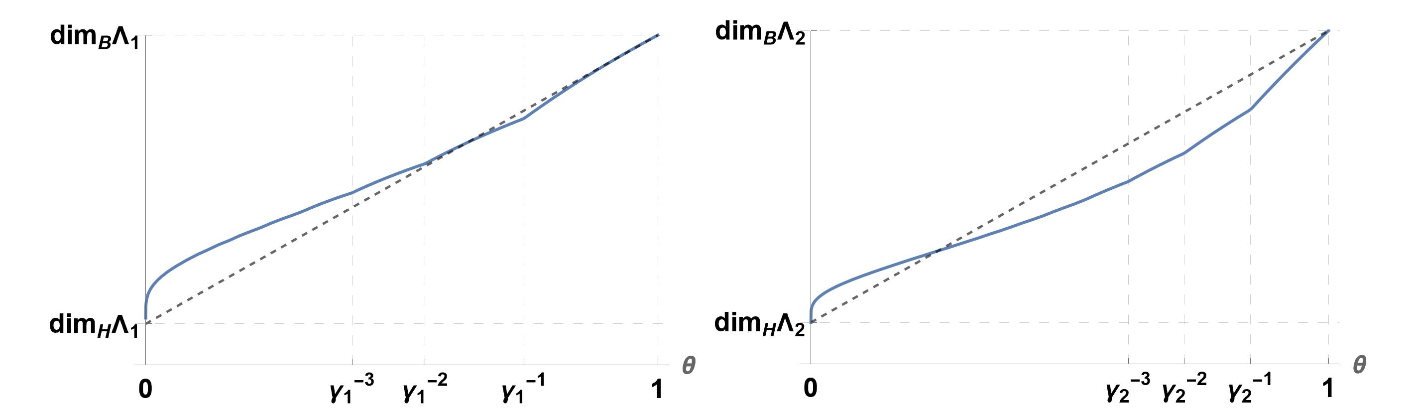
Figure 2. Parameters $n=100$ and $\mathbf{N}=(51,50,50,50,50,50)$ are the same in each example, only $m$ varies from $30$ on left to $50$ on right.

Example 2.12.

Consider two Bedford–McMullen carpets $\Lambda$ and $\Lambda^{\prime}$ with $m=M=32$ and $n=243$ and the following parameters:

$$\Lambda \colon\qquad M_{0}=3,\quad\{N_{1},N_{2},N_{3}\}=\{27,3,1\}\text{ and }\{R_{1},R_{2},R_{3}\}=\{2,11,19\},$$

$$\Lambda^{\prime} \colon\qquad M^{\prime}_{0}=3,\quad\{N^{\prime}_{1},N^{\prime}_{2},N^{\prime}_{3}\}=\{27,9,1\}\text{ and }\{R^{\prime}_{1},R^{\prime}_{2},R^{\prime}_{3}\}=\{1,6,25\}.$$

Then

• There exists $\theta\in(0,1)$ with $\dim_{\,\theta}\Lambda\neq\dim_{\,\theta}\Lambda^{\prime}$ (by part (5) of Theorem 2.4, since all $R_{\hat{\imath}}/R^{\prime}_{\hat{\imath}}$ are different)

• We have $\dim\Lambda=\dim\Lambda^{\prime}$ where $\dim$ can be any of the Hausdorff, box, packing, Assouad, quasi-Assouad, lower, quasi-lower or modified lower dimensions, or the Assouad spectrum or lower spectrum for any fixed $\theta\in(0,1)$. This holds since $N=106$, $\max_{1\leq i\leq 3}N_{i}=\max_{1\leq i\leq 3}N^{\prime}_{i}=27$, $\min_{1\leq i\leq M}N_{i}=\min_{1\leq i\leq M}N^{\prime}_{i}=1$, so we can use (1.2) and [22, Corollary 5.3] to show that the Hausdorff and modified lower dimensions are equal, and the formulae in [22] for the other dimensions.

Therefore $\Lambda$ and $\Lambda^{\prime}$ are not bi-Lipschitz equivalent but this is revealed only by the intermediate dimensions, not by any of the other dimensions mentioned above. If all the rectangles are chosen in a specific row, then neither $\Lambda$ nor $\Lambda^{\prime}$ is totally disconnected, so [39, Corollary 1.1] does not apply. Figure 3 shows the plots of $\dim_{\,\theta}\Lambda$ (blue) and $\dim_{\,\theta}\Lambda^{\prime}$ (orange) side-by-side on the left and the ratio $\dim_{\,\theta}\Lambda^{\prime}/\dim_{\,\theta}\Lambda$ on the right.

We can use Hölder distortion to obtain a quantitative improvement of the assertion that $\Lambda$ and $\Lambda^{\prime}$ are not bi-Lipschitz equivalent. Assume $f\colon\Lambda^{\prime}\to\mathbb{R}^{2}$ is $\alpha$-Hölder with $f(\Lambda^{\prime})\supseteq\Lambda$. Then the optimal value of $\theta$ to consider is $\theta=\gamma^{-2}=\left(\frac{\log 2}{\log 3}\right)^{2}\approx 0.40$, see right hand side of Figure 3. Then by (1.1),

$$\alpha\leq\frac{\dim_{\,\gamma^{-2}}\Lambda^{\prime}}{\dim_{\,\gamma^{-2}}f(\Lambda^{\prime})}\leq\frac{\dim_{\,\gamma^{-2}}\Lambda^{\prime}}{\dim_{\,\gamma^{-2}}\Lambda}<0.9995,$$

with the last inequality computed numerically using Theorem 2.1.

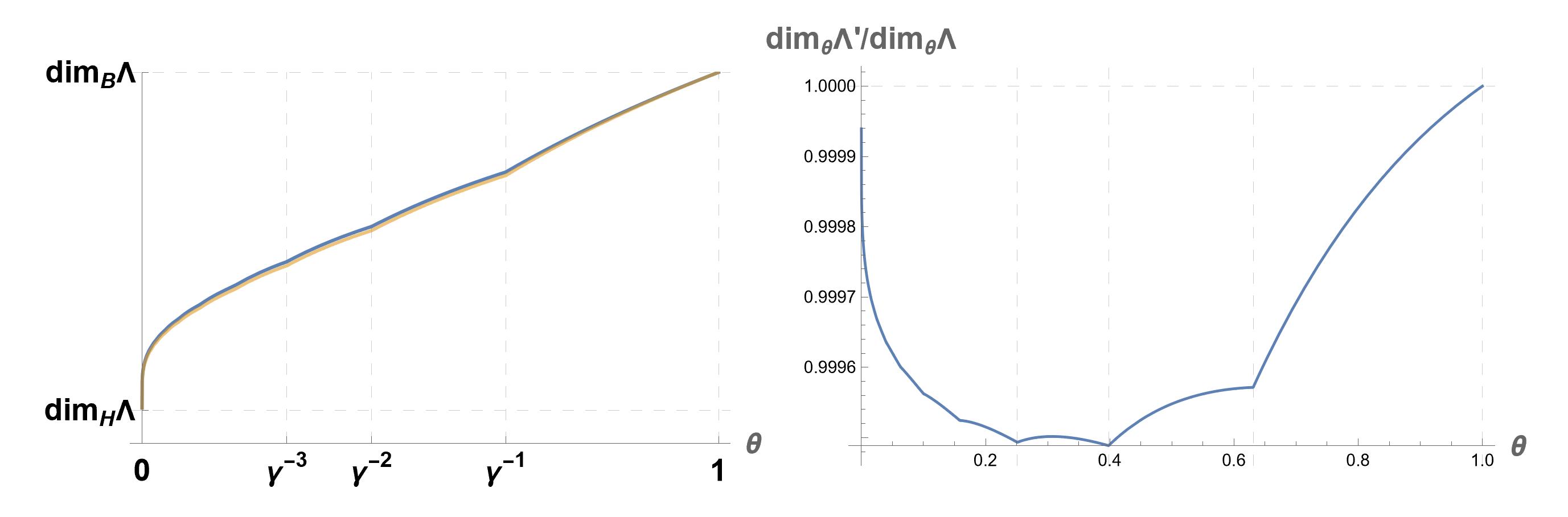
Figure 3. Left: plot of $\dim_{\,\theta}\Lambda$ (blue) and $\dim_{\,\theta}\Lambda^{\prime}$ (orange) from Example 2.12. Right: ratio of $\dim_{\,\theta}\Lambda^{\prime}/\dim_{\,\theta}\Lambda$ for $\theta\geq\gamma^{-35}$.

Fraser and Yu [24, Proposition 3.4] proved a similar result to Example 2.12 for the Assouad spectrum. Observe that if $\Lambda$ and $\Lambda^{\prime}$ are two carpets with non-uniform fibres which have the same intermediate dimensions for all $\theta\in(0,1)$, then $\dim\Lambda=\dim\Lambda^{\prime}$, where $\dim$ can be any other dimension mentioned in Example 2.12. Indeed, $\Lambda$ and $\Lambda^{\prime}$ can be defined on the same grid, on which part (5) of Theorem 2.4 holds, which implies equality of dimensions using the formulae in [22].

Example 2.13.

Using Proposition 2.10, the rate function (2.1) can be expressed explicitly when the carpet $\Lambda$ has just two different column types, meaning that $M_{0}=2$ using notation from Section 2.3. We calculate the entropy maximising vector $\mathbf{Q}^{*}_{t}\in\mathcal{P}_{M}$ defined in (2.9).

Let $\mathbf{q}=(q_{1},\ldots,q_{M_{0}})\in\mathcal{P}_{M_{0}}$. Entropy is increased the more uniform a vector is, hence it is enough to consider vectors $\mathbf{p}\in\mathcal{P}_{M}$ satisfying (2.9) of the form

$$p_{\hat{\imath}}=q_{j}/R_{j},\;\text{ if the }\hat{\imath}\text{-th non-empty column has }N_{j}\text{ number of maps},$$ (2.11)

in other words measure is distributed uniformly amongst columns with the same number of maps. As a result, the linear constraints in (2.9) can be rewritten as

$$1=\sum_{j=1}^{M_{0}}q_{j}\,\;\text{ and }\;\,t=\sum_{j=1}^{M_{0}}q_{j}\log N_{j}.$$ (2.12)

In particular, if $M_{0}=2$, then there is a single vector $(q^{*}_{1},q^{*}_{2})$ which satisfies (2.12),

$$q^{*}_{1}=\frac{t-\log N_{2}}{\log(N_{1}/N_{2})}\;\;\text{ and }\;\;q^{*}_{2}=\frac{\log N_{1}-t}{\log(N_{1}/N_{2})},$$

where recall $N_{1}>N_{2}$. Using (2.11), we can now calculate the entropy

$$H(\mathbf{Q}^{*}_{t}) =-\sum_{j=1}^{M_{0}}q^{*}_{j}\log(q^{*}_{j}/R_{j})$$

$$=\frac{-1}{\log(N_{1}/N_{2})}\left(\!\!(t-\log N_{2})\log\frac{t-\log N_{2}}{R_{1}\log(N_{1}/N_{2})}+(\log N_{1}-t)\log\frac{\log N_{1}-t}{R_{2}\log(N_{1}/N_{2})}\!\right)$$

and conclude from Proposition 2.10 that $I(t)=\log M-H(\mathbf{Q}^{*}_{t})$.

Example 2.14 (using the parameters from Rao, Yang and Zhang’s [39], Example 1.2).

Consider two Bedford–McMullen carpets defined on the same grid with $m=8$, $n=27$ and the following parameters:

$$\Lambda:\qquad M_{0}=2,\quad\{N_{1},N_{2}\}=\{6,3\}\mbox{ and }\{R_{1},R_{2}\}=\{1,1\},$$

$$\Lambda^{\prime}:\qquad M_{0}^{\prime}=2,\quad\{N_{1}^{\prime},N_{2}^{\prime}\}=\{2,1\}\mbox{ and }\{R_{1}^{\prime},R_{2}^{\prime}\}=\{2,2\}.$$

Then condition (5) from Theorem 2.4 holds, so $\dim_{\,\theta}\Lambda=\dim_{\,\theta}\Lambda^{\prime}$ for all $\theta\in[0,1]$, despite the fact that the carpets are defined on the same grid with different parameters. This is only possible because the number of non-empty columns is different.

Question 2.15.

Suppose two Bedford–McMullen carpets both have non-uniform vertical fibres, are defined on the same grid, and are bi-Lipschitz equivalent. Does it follow that both carpets must have identical parameters $(M_{0},N_{1},\ldots,N_{M_{0}},R_{1},\ldots,R_{M_{0}})$?

Example 2.16.

Consider the two carpets $\Lambda$ and $\Lambda^{\prime}$ with parameters

$$\Lambda:\qquad n=36,\quad m=6,\quad M=M_{0}=2,\quad\{N_{1},N_{2}\}=\{9,6\}\mbox{ and }\{R_{1},R_{2}\}=\{1,1\}$$

$$\Lambda^{\prime}:\qquad n=36,\quad m=4,\quad M=M_{0}=2,\quad\{N_{1},N_{2}\}=\{6,4\}\mbox{ and }\{R_{1},R_{2}\}=\{1,1\}.$$

Then it can be checked from Theorem 2.1 that $\dim_{\,\theta}\Lambda=\dim_{\,\theta}\Lambda^{\prime}$ for all $\theta\in[1/2,1]$, but not for the whole range of $\theta$; by Theorem 2.4 this is only possible because the carpets are defined on different grids. By Corollary 2.3, the graph of $\dim_{\,\theta}\Lambda$ has a phase transition at $\theta=1/2$ but the graph of $\dim_{\,\theta}\Lambda^{\prime}$ does not, see Figure 4.

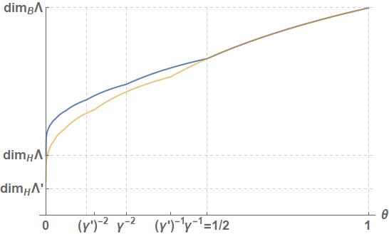
Figure 4. Plots of the intermediate dimensions of carpets in Example 2.16.

Remark 2.17.

All figures were created using Wolfram Mathematica 12.3 keeping simple implementation in mind and not necessarily efficiency. For a fixed $\theta\in(0,1)$, the value of $\dim_{\,\theta}\Lambda$ was approximated by taking $2^{25}$ equally spaced points in the interval $(\dim_{\mathrm{H}}\Lambda,\dim_{\mathrm{B}}\Lambda)$ and choosing the point $s(\theta)$ for which the expression in (2.4) was closest to $0$.

3. Proof of Proposition 2.10

Recall notation from Section 2. Assume $s\in(\underline{s},\overline{s})$ and that $(s,t)$ are related by (2.10). We prove Proposition 2.10 in four steps:

Step 1:

$\overline{P}(s)\leq H(\mathbf{Q}^{*}_{t})$,

Step 2:

$H(\mathbf{Q}^{*}_{t})\leq\underline{P}(s)$ and

Step 3:

$H(\mathbf{Q}^{*}_{t})=\log M-I(t)$.

Step 4:

$I(t)=-(\log m)f_{\nu}\left(\frac{\log N}{\log m}-\left(\frac{1}{\log m}-\frac{1}{\log n}\right)t\right)+\frac{t}{\gamma}+\log M$.

Some of the assertions we will prove as part of the proof of these steps will not follow from the statements of these steps, and will be important in their own right when we prove Theorem 2.1. Before proving these steps in separate subsections, we need some preliminaries. This is where we introduce the probability vectors $\mathbf{P}^{*}_{t}$ and $\mathbf{Q}^{*}_{t}$ which have certain optimising properties and recall some facts from the method of types.

3.1. Preliminaries

If $k,k_{1},k_{2}\in\mathbb{N}$ satisfy $0\leq k_{1}<k_{2}\leq k$, and $\boldsymbol{\hat{\imath}}\in\{1,\ldots,M\}^{k}$, then we define the average

$$\tau(\boldsymbol{\hat{\imath}},k_{1},k_{2})\coloneqq\max\Bigg{\{}\underline{t},\frac{1}{k_{2}-k_{1}}\sum_{j=k_{1}+1}^{k_{2}}\log N_{\hat{\imath}_{j}}\Bigg{\}}.$$ (3.1)

Recall, $\mathcal{P}_{M}$ denotes the set of probability vectors on $[M]=\{1,\ldots,M\}$ and we introduced two distinguished probability vectors

$$\mathbf{P}\coloneqq(N_{1}/N,\ldots,N_{M}/N)\;\text{ and }\;\mathbf{Q}\coloneqq(1/M,\ldots,1/M).$$

We remind the reader that the Kullback–Leibler divergence, also known as the relative entropy of $\mathbf{p}\in\mathcal{P}_{M}$ with respect to $\mathbf{q}\in\mathcal{P}_{M}$ is

$$H(\mathbf{p}\|\mathbf{q})\coloneqq\sum_{\hat{\imath}=1}^{M}p_{\hat{\imath}}\log(p_{\hat{\imath}}/q_{\hat{\imath}})=-H(\mathbf{p})-\sum_{\hat{\imath}=1}^{M}p_{\hat{\imath}}\log q_{\hat{\imath}}.$$

It is asymmetric and $H(\mathbf{p}\|\mathbf{q})\geq 0$ with equality if and only if $\mathbf{p}=\mathbf{q}$. In particular,

$$H(\mathbf{p}\|\mathbf{P})=\log N-H(\mathbf{p})-\sum_{\hat{\imath}=1}^{M}p_{\hat{\imath}}\log N_{\hat{\imath}}\qquad\text{ and }\qquad H(\mathbf{p}\|\mathbf{Q})=\log M-H(\mathbf{p}).$$ (3.2)

Recall, $\underline{t}=\overline{\log\mathbf{N}}$ and $\overline{t}=\log N-H(\mathbf{P})$ and let $t\in(\underline{t},\overline{t})$. We divide the set $\mathcal{P}_{M}$ into two parts:

$$\mathcal{G}_{t}\coloneqq\bigg{\{}\mathbf{p}\in\mathcal{P}_{M}:\,\sum_{\hat{\imath}=1}^{M}p_{\hat{\imath}}\log N_{\hat{\imath}}\leq t\bigg{\}}\;\text{ and }\;\mathcal{F}_{t}\coloneqq\bigg{\{}\mathbf{p}\in\mathcal{P}_{M}:\,\sum_{\hat{\imath}=1}^{M}p_{\hat{\imath}}\log N_{\hat{\imath}}\geq t\bigg{\}},$$ (3.3)

so that $\mathcal{E}_{t}\coloneqq\mathcal{G}_{t}\cap\mathcal{F}_{t}=\big{\{}\mathbf{p}\in\mathcal{P}_{M}:\,\sum_{\hat{\imath}}p_{\hat{\imath}}\log N_{\hat{\imath}}=t\big{\}}$. The reason for doing this will become clear in the proof of Step 1, see (3.10). Since $t>\underline{t}$, it follows that $\mathbf{Q}\in\mathcal{G}_{t}\setminus\mathcal{E}_{t}$, whereas $\mathbf{P}\in\mathcal{F}_{t}\setminus\mathcal{E}_{t}$ because $t<\overline{t}=\sum_{\hat{\imath}=1}^{M}P_{\hat{\imath}}\log N_{\hat{\imath}}$.

Lemma 3.1.

Assume $t\in(\underline{t},\overline{t})$ and $\mathbf{p}\in\mathcal{E}_{t}$. Then

$$H(\mathbf{p}\|\mathbf{P})=H(\mathbf{p}\|\mathbf{Q})+\log(N/M)-t.$$

Proof.

Let $\mathbf{p}\in\mathcal{E}_{t}$. Assume $N^{\prime}_{1}<N^{\prime}_{2}<\cdots<N^{\prime}_{M_{0}}$ denote the different values that the set $\{N_{1},\ldots,N_{M}\}$ takes. For $1\leq j\leq M_{0}$ let $I_{j}\coloneqq\{\hat{\imath}\in[M]:\,N_{\hat{\imath}}=N^{\prime}_{j}\}$ and $q_{j}\coloneqq\sum_{\hat{\imath}\in I_{j}}p_{\hat{\imath}}$. Then,

$$1=\sum_{\hat{\imath}=1}^{M}p_{\hat{\imath}}=\sum_{j=1}^{M_{0}}q_{j}\,\;\text{ and }\;\,t=\sum_{\hat{\imath}=1}^{M}p_{\hat{\imath}}\log N_{\hat{\imath}}=\sum_{j=1}^{M_{0}}q_{j}\log N^{\prime}_{j}.$$

This is a linear system of equations for $\{q_{j}\}_{j=1}^{M_{0}}$. Straightforward Gaussian elimination yields

$$\left[\begin{array}[]{@{}ccc|c@{}}1&\dots&1&1\\ \log N^{\prime}_{1}&\dots&\log N^{\prime}_{M_{0}}&t\end{array}\right]\;\sim\;\left[\begin{array}[]{@{}ccccc|c@{}}1&1&1&\dots&1&1\\ 0&1&\frac{\log(N^{\prime}_{3}/N^{\prime}_{1})}{\log(N^{\prime}_{2}/N^{\prime}_{1})}&\dots&\frac{\log(N^{\prime}_{M_{0}}/N^{\prime}_{1})}{\log(N^{\prime}_{2}/N^{\prime}_{1})}&\frac{t-\log N^{\prime}_{1}}{\log(N^{\prime}_{2}/N^{\prime}_{1})}\end{array}\right].$$

Thus, for any solution $(q_{1},\ldots,q_{M_{0}})$, we see that $q_{3},\ldots,q_{M_{0}}$ are free variables, and moreover

$$q_{2}=\frac{1}{\log(N^{\prime}_{2}/N^{\prime}_{1})}\bigg{(}t-\sum_{j=3}^{M_{0}}q_{j}\log N^{\prime}_{j}-\bigg{(}1-\sum_{j=3}^{M_{0}}q_{j}\bigg{)}\log N^{\prime}_{1}\bigg{)}$$

and $q_{1}=1-q_{2}-\sum_{j=3}^{M_{0}}q_{j}$. It now follows by a straightforward calculation that $\sum_{j=1}^{M_{0}}q_{j}\log N^{\prime}_{j}=t$. By (3.2), the result follows. ∎

Let us introduce $\mathbf{P}^{*}_{t}\in\mathcal{G}_{t}$, $\mathbf{Q}^{*}_{t}\in\mathcal{F}_{t}$ defined by

$$H(\mathbf{P}^{*}_{t}\|\mathbf{P})=\inf_{\mathbf{p}\in\mathcal{G}_{t}}H(\mathbf{p}\|\mathbf{P})\qquad\text{ and }\qquad H(\mathbf{Q}^{*}_{t}\|\mathbf{Q})=\inf_{\mathbf{q}\in\mathcal{F}_{t}}H(\mathbf{q}\|\mathbf{Q}).$$ (3.4)

Due to (3.2) and Lemma 3.2, this definition of $\mathbf{Q}^{*}_{t}$ is equivalent to (2.9).

Lemma 3.2.

Assume $t\in(\underline{t},\overline{t})$. Both $\mathbf{P}^{*}_{t}$ and $\mathbf{Q}^{*}_{t}$ are well defined. Moreover, $\mathbf{P}^{*}_{t},\mathbf{Q}^{*}_{t}\in\mathcal{E}_{t}$ and

$$H(\mathbf{P}^{*}_{t}\|\mathbf{P})=H(\mathbf{Q}^{*}_{t}\|\mathbf{Q})+\log(N/M)-t.$$ (3.5)

Proof.

Both $H(\cdot\,\|\mathbf{P})$ and $H(\cdot\,\|\mathbf{Q})$ are continuous on the domain $\mathcal{P}_{M}$, moreover $\mathcal{G}_{t}$ and $\mathcal{F}_{t}$ are compact, hence both infima are attained. Next, $\nabla H(\mathbf{q}\|\mathbf{Q})=\underline{0}$ if and only if $\mathbf{q}=\mathbf{Q}\in\mathcal{G}_{t}\setminus\mathcal{E}_{t}$, likewise, $\nabla H(\mathbf{p}\|\mathbf{P})=\underline{0}$ if and only if $\mathbf{p}=\mathbf{P}\in\mathcal{F}_{t}\setminus\mathcal{E}_{t}$. Continuity implies that necessarily $\mathbf{P}^{*}_{t},\mathbf{Q}^{*}_{t}$ are elements of the boundary $\mathcal{E}_{t}$. To conclude, Lemma 3.1 yields that

$$H(\mathbf{Q}^{*}_{t}\|\mathbf{P})=H(\mathbf{Q}^{*}_{t}\|\mathbf{Q})+\log(N/M)-t\leq H(\mathbf{P}^{*}_{t}\|\mathbf{Q})+\log(N/M)-t=H(\mathbf{P}^{*}_{t}\|\mathbf{P})\leq H(\mathbf{Q}^{*}_{t}\|\mathbf{P}),$$

so we have equality throughout. ∎

Remark 3.3.

The importance of choosing $t\in(\underline{t},\overline{t})$, or equivalently $s\in(\underline{s},\overline{s})$ is that in this case the hyperplane $\mathcal{E}_{t}$ separates $\mathbf{P}$ and $\mathbf{Q}$. Otherwise, either $H(\mathbf{P}^{*}_{t}\|\mathbf{P})=0$ or $H(\mathbf{Q}^{*}_{t}\|\mathbf{Q})=0$ and (3.5) does not necessarily hold.

Method of types

The method of types is an elementary tool developed to study discrete memoryless systems in information theory and has since found applications in for example hypothesis testing, combinatorics or large deviations, see [12] for some background. Kolossváry very recently used it to calculate the box dimension of Gatzouras–Lalley and Barański sponges in $\mathbb{R}^{d}$ [32].

Let $[M]=\{1,\ldots,M\}$ denote a finite alphabet and assume $\overline{\imath}=(i_{1},\ldots,i_{J})\in[M]^{J}$. For $J^{\prime}\leq J$, the type of $\overline{\imath}$ at level $J^{\prime}$ is the empirical probability vector

$$\boldsymbol{\tau}_{J^{\prime}}^{J}(\overline{\imath})=\frac{1}{J^{\prime}}\big{(}\#\{1\leq\ell\leq J^{\prime}:\,i_{\ell}=j\}\big{)}_{j\in[M]}.$$

When $J^{\prime}=J$, we simply write $\boldsymbol{\tau}_{J}(\overline{\imath})\coloneqq\boldsymbol{\tau}_{J}^{J}(\overline{\imath})$. The set of all possible types of $[M]^{J}$ is

$$\mathcal{T}_{J}=\big{\{}\mathbf{p}\in\mathcal{P}_{M}:\text{ there exists }\overline{\imath}\in[M]^{J}\text{ such that }\mathbf{p}=\boldsymbol{\tau}_{J}(\overline{\imath})\big{\}},$$

and for $J^{\prime}\leq J$, the type class of $\mathbf{p}\in\mathcal{T}_{J^{\prime}}$ amongst $[M]^{J}$ is the set

$$T_{J^{\prime}}^{J}(\mathbf{p})=\big{\{}\overline{\imath}\in[M]^{J}:\,\boldsymbol{\tau}_{J^{\prime}}^{J}(\overline{\imath})=\mathbf{p}\big{\}}.$$

Similarly, $T_{J}(\mathbf{p})\coloneqq T_{J}^{J}(\mathbf{p})$. We use the following two simple facts:

$$\#\mathcal{T}_{J}\leq(J+1)^{M}$$ (3.6)

and for any type class

$$\big{(}J+1\big{)}^{-M}e^{J\cdot H(\mathbf{p})}\leq\#T_{J}(\mathbf{p})\leq e^{J\cdot H(\mathbf{p})},$$ (3.7)

see [14, Lemmas 2.1.2 and 2.1.8]. The importance of (3.6) is that $\#\mathcal{T}_{J}$ grows only polynomially in $J$, on the other hand, the exponential terms in (3.7) are the same in both the lower and upper bounds. Since we are looking for critical exponents, sub-exponential multiplicative terms do not influence our calculations. To simplify notation, we write $f(J)\asymp g(J)$ if the exponential rate of growth of $f(J)>0$ and $g(J)>0$ exist and are equal to each other, so

$$f(J)\asymp g(J)\;\Longleftrightarrow\;\lim_{J\to\infty}\frac{1}{J}\log f(J)=\lim_{J\to\infty}\frac{1}{J}\log g(J).$$

In particular, if $f(J)$ is sub-exponential in $J$, then $f(J)\asymp 1$.

The set $\mathcal{T}_{J}$ is a discrete set with polynomially many points which becomes dense in $\mathcal{P}_{M}$ as $J\to\infty$. For $\mathbf{p}\in\mathcal{P}_{M}$ let $\mathbf{p}_{J}$ denote the ‘best approximation’ of $\mathbf{p}$ in $\mathcal{T}_{J}$, in the sense that $\|\mathbf{p}-\mathbf{p}_{J}\|=\min_{\mathbf{q}\in\mathcal{T}_{J}}\|\mathbf{p}-\mathbf{q}\|$, where we can take any norm. If there are many such $\mathbf{p}_{J}$ then we can choose the one with smallest coordinates when ordered lexicographically. For large enough $J$, $\|\mathbf{p}-\mathbf{p}_{J}\|$ is arbitrarily small. In particular, property (3.7) and the continuity of the entropy imply that $\#T_{J}(\mathbf{p}_{J})\asymp e^{J\cdot H(\mathbf{p})}$.

3.2. Proof of Step 1

Since $\min_{k\in\{0,1,\ldots,J\}}\psi_{\overline{\imath}|k}(s)\leq\min\{1,\psi_{\overline{\imath}|J}(s)\}$, recall definition of $\psi_{\overline{\imath}|k}(s)$ from (2.7),

$$\Psi_{J}(s)\leq\#\big{\{}\overline{\imath}\in[M]^{J}:\,1<\psi_{\overline{\imath}|J}(s)\big{\}}+\sum_{\overline{\imath}\in[M]^{J}:\,\psi_{\overline{\imath}|J}(s)\leq 1}\psi_{\overline{\imath}|J}(s).$$ (3.8)

Lemma 3.4.

Assume $t\in(\underline{t},\max_{1\leq i\leq N}\log N_{i})$ and $(s,t)$ are related by (2.10). Then

$$\#\big{\{}\overline{\imath}\in[M]^{J}:\,1<\psi_{\overline{\imath}|J}(s)\big{\}}\asymp e^{J\cdot H(\mathbf{Q}^{*}_{t})}.$$

Proof.

Using (2.7), straightforward algebraic manipulations show us that

$$\psi_{\overline{\imath}|J}(s)\leq 1\;\Longleftrightarrow\;\frac{1}{J}\sum_{\ell=1}^{J}\log N_{i_{\ell}}\leq\Big{(}s-\frac{\log M}{\log m}\Big{)}\cdot\log n=t.$$ (3.9)

This explains why the relationship between $s$ and $t$ was introduced in (2.10) in that particular form. For any given word $\overline{\imath}\in[M]^{J}$, the average of the $\log N_{i_{\ell}}$ does not depend on the particular order of the symbols in $\overline{\imath}$, just on the relative frequency of each symbol. In other words, only the type $\boldsymbol{\tau}_{J}(\overline{\imath})=(\tau_{J,1}(\overline{\imath}),\ldots,\tau_{J,M}(\overline{\imath}))$ of $\overline{\imath}$ matters,

$$\psi_{\overline{\imath}|J}(s)\leq 1\;\Longleftrightarrow\;\sum_{\hat{\imath}=1}^{M}\tau_{J,\hat{\imath}}(\overline{\imath})\log N_{\hat{\imath}}\leq t.$$

This reduces the problem back to a condition on probability vectors $\mathbf{p}\in\mathcal{P}_{M}$. This is the reason why we introduced $\mathcal{G}_{t}$ and $\mathcal{F}_{t}$ the way we did in (3.3). We now see that

$$\psi_{\overline{\imath}|J}(s)\leq 1\;\Longleftrightarrow\;\boldsymbol{\tau}_{J}(\overline{\imath})\in\mathcal{G}_{t}.$$ (3.10)

We are now ready to determine the exponential rate of growth of the two terms in (3.8) separately by grouping together words according to type class. Let $\mathbf{Q}^{*}_{t,J}\in(\mathcal{F}_{t}\cap\mathcal{T}_{J})$ be the type for which $H(\mathbf{Q}^{*}_{t,J})=\max_{\mathbf{q}\in(\mathcal{F}_{t}\cap\mathcal{T}_{J})}H(\mathbf{q})$ (if there is more than one such vector then we can choose the smallest lexicographically). Then

$$(J+1)^{-M}e^{J\cdot H(\mathbf{Q}^{*}_{t,J})}\leq\#\big{\{}\overline{\imath}\in[M]^{J}:\,1<\psi_{\overline{\imath}|J}(s)\big{\}}=\sum_{\mathbf{q}\in(\mathcal{F}_{t}\cap\mathcal{T}_{J})}\#T_{J}(\mathbf{q})\leq\#\mathcal{T}_{J}\cdot e^{J\cdot H(\mathbf{Q}^{*}_{t,J})},$$

where we used (3.7) for the two inequalities. As $J\to\infty$, the set $\mathcal{T}_{J}$ becomes dense in $\mathcal{P}_{M}$, as a result, $\|\mathbf{Q}^{*}_{t,J}-\mathbf{Q}^{*}_{t}\|\to 0$, in particular, $H(\mathbf{Q}^{*}_{t,J})\to H(\mathbf{Q}^{*}_{t})$. Hence, it follows from (3.6) that $\#\big{\{}\overline{\imath}\in[M]^{J}:\,1<\psi_{\overline{\imath}|J}(s)\big{\}}\asymp e^{J\cdot H(\mathbf{Q}^{*}_{t})}$. An alternative way to see this would be to let $X_{1},X_{2},\ldots,X_{J},\ldots$ be a sequence of independent random variables all uniformly distributed on the set $\{\log N_{1},\ldots,\log N_{M}\}$. Then

$$\#\big{\{}\overline{\imath}\in[M]^{J}:\,1<\psi_{\overline{\imath}|J}(s)\big{\}}\stackrel{{\scriptstyle\eqref{eq:309}}}{{=}}M^{J}\mathds{P}\left(\sum_{i=1}^{J}X_{i}>tJ\right)\asymp M^{J}e^{-J\cdot I(t)}=e^{J\cdot H(\mathbf{Q}^{*}_{t})},$$

where we used Cramér’s theorem for the asymptotic equality and Step 3 for the final equality. ∎

Lemma 3.5.

Assume $s\in(\underline{s},\overline{s})$ and $(s,t)$ are related by (2.10). Then

$$\sum_{\overline{\imath}\in[M]^{J}:\,\psi_{\overline{\imath}|J}(s)\leq 1}\psi_{\overline{\imath}|J}(s)\asymp e^{J\cdot H(\mathbf{Q}^{*}_{t})}.$$

Proof.

If $\overline{\imath}\in T_{J}(\mathbf{p})$, then

$$\psi_{\overline{\imath}|J}(s)=M^{J\log_{m}n}n^{-sJ}\cdot\prod_{\hat{\imath}=1}^{M}N_{\hat{\imath}}^{p_{\hat{\imath}}J}=e^{J\left(\left(\frac{\log M}{\log m}-s\right)\cdot\log n+\sum_{\hat{\imath}}p_{\hat{\imath}}\log N_{\hat{\imath}}\right)}=e^{J(-t+\sum_{\hat{\imath}}p_{\hat{\imath}}\log N_{\hat{\imath}})}.$$ (3.11)

Using (3.7) and (3.2),

$$\#T_{J}(\mathbf{p})\cdot\psi_{\overline{\imath}|J}(s)\asymp e^{J(-t+\sum_{\hat{\imath}}p_{\hat{\imath}}\log N_{\hat{\imath}}+H(\mathbf{p}))}=e^{J\left(-t+\log N-H(\mathbf{p}\|\mathbf{P})\right)}.$$

Similarly to $\mathbf{Q}^{*}_{t,J}$, let $\mathbf{P}^{*}_{t,J}\in(\mathcal{G}_{t}\cap\mathcal{T}_{J})$ satisfy $H(\mathbf{P}^{*}_{t,J}\|\mathbf{P})=\min_{\mathbf{p}\in(\mathcal{G}_{t}\cap\mathcal{T}_{J})}H(\mathbf{p}\|\mathbf{P})$. We have $H(\mathbf{P}^{*}_{t,J}\|\mathbf{P})\to H(\mathbf{P}^{*}_{t}\|\mathbf{P})$ as $J\to\infty$. Then

$$\sum_{\overline{\imath}\in[M]^{J}:\,\psi_{\overline{\imath}|J}(s)\leq 1}\psi_{\overline{\imath}|J}(s)=\sum_{\mathbf{p}\in(\mathcal{G}_{t}\cap\mathcal{T}_{J})}\sum_{\overline{\imath}\in T_{J}(\mathbf{p})}\psi_{\overline{\imath}|J}(s)\asymp e^{J\left(-t+\log N-H(\mathbf{P}^{*}_{t,J}\|\mathbf{P})\right)}.$$

Using (3.5) and (3.2) in the exponent, $-t+\log N-H(\mathbf{P}^{*}_{t}\|\mathbf{P})=\log M-H(\mathbf{Q}^{*}_{t}\|\mathbf{Q})=H(\mathbf{Q}^{*}_{t})$, and the assertion follows. ∎

Note the importance of the assumption $t<\overline{t}$ in the proof of Lemma 3.5. Lemmas 3.4 and 3.5 and (3.8) immediately imply that $\overline{P}(s)\leq H(\mathbf{Q}^{*}_{t})$.

3.3. Proof of Step 2

This in fact holds for all $t\in(\underline{t},\max_{1\leq i\leq N}\log N_{i})$. Assume $(s,t)$ are related by (2.10). Fix $R\in\mathbb{N}$. For $J\in\mathbb{N}$, if $l\in\{0,1,\ldots,R-1\}$, let $J_{l,R}\coloneqq\lfloor(l+1)J/R\rfloor-\lfloor lJ/R\rfloor$. We introduce

$$\begin{split}S_{t,J,R}\coloneqq\big{\{}\,\overline{\imath}=(i_{1},\ldots,i_{J})\in[M]^{J}:&(i_{\lfloor lJ/R\rfloor+1},\ldots,i_{\lfloor(l+1)J/R\rfloor})\in T_{J_{l,R}}(\mathbf{Q}^{*}_{t,J_{l,R}})\\ &\mbox{ for all }l\in\{0,1,\ldots,R-1\}\,\big{\}}.\end{split}$$ (3.12)

Then

$$\#S_{t,J,R}=\prod_{l=0}^{R-1}\#T_{J_{l,R}}(\mathbf{Q}^{*}_{t,J_{l,R}})\stackrel{{\scriptstyle\eqref{eq:206}}}{{\asymp}}\prod_{l=0}^{R-1}e^{J_{l,R}\cdot H(\mathbf{Q}^{*}_{t,J_{l,R}})}\asymp e^{J\cdot H(\mathbf{Q}^{*}_{t})}=e^{J(\log M-I(t))}$$ (3.13)

as $J\to\infty$, using Step 3 of Proposition 2.10 in the last step. Suppose $(i_{1},\ldots,i_{J})\in S_{t,J,R}$. For all $l\in\{0,1,\ldots,R-1\}$, $\mathbf{Q}^{*}_{t,J_{l,R}}\to\mathbf{Q}^{*}_{t}\in\mathcal{E}_{t}$, so $\psi_{(i_{\lfloor lJ/R\rfloor+1},\ldots,i_{\lfloor(l+1)J/R\rfloor})|J_{l,R}}(s)\asymp 1$ as $J\to\infty$ by (3.9). Let $J^{\prime}\in\mathbb{N}$ be large enough that for all $J\geq J^{\prime}$ and $l\in\{0,1,\ldots,R-1\}$, $\psi_{(i_{\lfloor lJ/R\rfloor+1},\ldots,i_{\lfloor(l+1)J/R\rfloor})|J_{l,R}}(s)\geq e^{-\overline{t}J_{l,R}/R}$. Assume $J\geq J^{\prime}$. For each $k\in\{1,\ldots,J\}$ let $\mathbf{p}(k)$ denote the type class of $(i_{1},\ldots,i_{k})$ and let $l\in\{0,1,\ldots,R-1\}$ be such that $\lfloor lJ/R\rfloor<k\leq\lfloor(l+1)J/R\rfloor$. Then

$$\begin{split}\psi_{(i_{1},\ldots,i_{k})|k}(s)\stackrel{{\scriptstyle\eqref{eq:308}}}{{=}}e^{k(-t+\sum_{\hat{\imath}}p_{\hat{\imath}}(k)\log N_{\hat{\imath}})}&\geq e^{\lfloor lJ/R\rfloor(-t+\sum_{\hat{\imath}}p_{\hat{\imath}}(\lfloor lJ/R\rfloor)\log N_{\hat{\imath}})}e^{(\lfloor lJ/R\rfloor-k)t}\\ &\geq\psi_{(i_{1},\ldots,i_{\lfloor lJ/R\rfloor})|\lfloor lJ/R\rfloor}(s)e^{-2\overline{t}J/R}\\ &\geq e^{-3\overline{t}J/R},\end{split}$$ (3.14)

where in the last step we use that by (2.7),

$$\psi_{(i_{1},\ldots,i_{A},i_{A+1},\ldots,i_{A+A^{\prime}})|A+A^{\prime}}(s)=\psi_{(i_{1},\ldots,i_{A})|A}(s)\psi_{(i_{A+1},\ldots,i_{A+A^{\prime}})|A^{\prime}}(s).$$

Therefore

$$\underline{P}(s)=\liminf_{J\to\infty}\frac{1}{J}\log\Psi_{J}(s)\geq\liminf_{J\to\infty}\frac{1}{J}\log\sum_{\overline{\imath}\in S_{t,J,R}}\min_{k\in\{0,1,\ldots,J\}}\psi_{\overline{\imath}|k}(s)\geq H(\mathbf{Q}^{*}_{t})-3\overline{t}/R.$$

Since $R\in\mathbb{N}$ was arbitrary, the assertion $\underline{P}(s)\geq H(\mathbf{Q}^{*}_{t})$ follows.

3.4. Proof of Step 3

This is a standard argument in large deviations theory, and in fact holds for all $t\in(\underline{t},\max_{1\leq i\leq M}\log N_{i})$. We include a sketch of it for the convenience of the reader. An alternative approach would be to use Lagrange multipliers.

Let $\mathbf{I}=I_{1},I_{2},\ldots$ be an infinite sequence of independent and identically distributed random variables on the set $\{1,\ldots,M\}$ according to $\mathbf{q}\in\mathcal{P}_{M}$. Let $\mathds{P}_{\mathbf{q}}\coloneqq\mathbf{q}^{\mathds{N}}$ denote the product measure corresponding to the distribution of the sequence $\mathbf{I}$. Then $\boldsymbol{\tau}_{J}(\mathbf{I})$, the type of $(I_{1},\ldots,I_{J})$, is a vector-valued random variable. For any $\mathbf{p}\in\mathcal{T}_{J}$,

$$(J+1)^{-M}e^{-J\cdot H(\mathbf{p}\|\mathbf{q})}\leq\mathds{P}_{\mathbf{q}}(\boldsymbol{\tau}_{J}(\mathbf{I})=\mathbf{p})\leq e^{-J\cdot H(\mathbf{p}\|\mathbf{q})},$$

see [14, Lemma 2.1.9]. Sanov’s theorem [14, Theorem 2.1.10] shows that the family of laws $\mathds{P}_{\mathbf{q}}(\boldsymbol{\tau}_{J}(\mathbf{I})\in\cdot)$ satisfies a large deviations principle with the rate function $H(\cdot\|\mathbf{q})$. In particular, for $\mathbf{q}=\mathbf{Q}=(1/M,\ldots,1/M)$ and the subset $\mathcal{F}_{t}$:

$$\mathds{P}_{\mathbf{Q}}(\boldsymbol{\tau}_{J}(\mathbf{I})\in\mathcal{F}_{t})\asymp e^{-J\inf_{\mathbf{q}\in\mathcal{F}_{t}}H(\mathbf{q}\|\mathbf{Q})}=e^{-JH(\mathbf{Q}^{*}_{t}\|\mathbf{Q})}.$$

Now define the random variable $X_{\ell}\coloneqq\log N_{I_{\ell}}$ and the averages $Y_{J}\coloneqq\frac{1}{J}\sum_{\ell=1}^{J}X_{\ell}$. Then

$$Y_{J}=\sum_{\hat{\imath}=1}^{M}\tau_{J,\hat{\imath}}(\mathbf{I})\cdot\log N_{\hat{\imath}}$$

is a continuous function of $\boldsymbol{\tau}_{J}(\mathbf{I})$. Hence, by the ‘contraction principle’ [14, Section 4.2.1], the rate function $I(t)$ of $\mathds{P}_{\mathbf{Q}}(Y_{J}\in\cdot)$ is equal to

$$I(t)=\inf\Big{\{}H(\mathbf{q}\|\mathbf{Q}):\,\sum_{\hat{\imath}=1}^{M}q_{\hat{\imath}}\log N_{\hat{\imath}}=t\Big{\}}.$$

In particular, Lemma 3.2 implies that

$$I(t)=\inf_{\mathbf{q}\in\mathcal{E}_{t}}H(\mathbf{q}\|\mathbf{Q})\stackrel{{\scriptstyle\eqref{eq:defineqstar}}}{{=}}H(\mathbf{Q}^{*}_{t}\|\mathbf{Q})\stackrel{{\scriptstyle\eqref{eq:32}}}{{=}}\log M-H(\mathbf{Q}^{*}_{t}).$$

3.5. Proof of Step 4

This is an application of [27, Theorem 1], and in fact holds for all $t\in(\min_{1\leq i\leq M}\log N_{i},\max_{1\leq i\leq M}\log N_{i})$. Indeed, by (2.5), for all $\lambda$ we have

$$\log\left(\frac{1}{M}\sum_{\hat{\imath}=1}^{M}N_{i}^{\lambda}\right)=(\log m)\left(\beta_{\nu}\left(\frac{\lambda-\gamma^{-1}}{(\log m)(\frac{1}{\log m}-\frac{1}{\log n})}\right)+\frac{(\lambda-\gamma^{-1})\frac{\log N}{\log m}}{(\log m)(\frac{1}{\log m}-\frac{1}{\log n})}\right)-\log M.$$

Taking the Legendre transform of each side and using standard properties of Legendre transforms and (2.1) and (2.6) proves Step 4. This completes the proof of Proposition 2.10.

4. Preliminaries to the proof of Theorem 2.1

Here we collect some notation and facts used in the proof of Theorem 2.1. Throughout the section, $\Lambda$ is a Bedford–McMullen carpet with non-uniform vertical fibres.

4.1. General theory

Following [10], for a bounded and non-empty set $F\subset\mathbb{R}^{d}$, $\theta\in(0,1)$ and $s\in[0,d]$, let us introduce

$$S_{\delta,\theta}^{s}(F)\coloneqq\inf\Big{\{}\sum_{i}\left|U_{i}\right|^{s}:\left\{U_{i}\right\}_{i}\text{ is a cover of }F\text{ such that }\delta^{1/\theta}\leq\left|U_{i}\right|\leq\delta\text{ for all }i\Big{\}}.$$ (4.1)

The motivation for introducing $S_{\delta,\theta}^{s}(F)$ is that from [10, Lemma 2.1] and the definitions of $\underline{\dim}_{\,\theta}F$ and $\overline{\dim}_{\,\theta}F$ it follows that

$$\underline{\dim}_{\,\theta}F=\text{ the unique }s\in[0,d]\text{ such that }\liminf_{\delta\searrow 0}\frac{\log S_{\delta,\theta}^{s}(F)}{-\log\delta}=0$$

and

$$\overline{\dim}_{\,\theta}F=\text{ the unique }s\in[0,d]\text{ such that }\limsup_{\delta\searrow 0}\frac{\log S_{\delta,\theta}^{s}(F)}{-\log\delta}=0.$$ (4.2)

For each $\theta\in(0,1)$, $\liminf_{\delta\searrow 0}\frac{\log S_{\delta,\theta}^{s}(F)}{-\log\delta}$ and $\limsup_{\delta\searrow 0}\frac{\log S_{\delta,\theta}^{s}(F)}{-\log\delta}$ are strictly decreasing and continuous functions of $s$. To bound $S_{\delta,\theta}^{s}(\Lambda)$ from above, we construct an efficient cover of $\Lambda$ in Section 5.3. The mass distribution principle is a useful tool to bound some dimension of a set from below by putting a measure on the set. For the matching lower bound, we will use the following version of the mass distribution principle for the intermediate dimensions of Falconer, Fraser and Kempton, [19, Proposition 2.2].

Proposition 4.1.

Let $F$ be a non-empty, bounded subset of $\mathbb{R}^{d}$, and let $\theta\in[0,1]$, $s\geq 0$, $\delta_{0}\in(0,1)$. Suppose that for all $\delta\in(0,\delta_{0})$ there exists a Borel measure $\mu_{\delta}$ with support $\mathrm{supp}(\mu)\subseteq F$ such that $\mu_{\delta}(U)\leq|U|^{s}$ for all Borel sets $U\subset\mathbb{R}^{d}$ with $\delta^{1/\theta}\leq|U|\leq\delta$. Then

$$\liminf_{\delta\searrow 0}\frac{\log S_{\delta,\theta}^{s}(F)}{-\log\delta}\geq\liminf_{\delta\searrow 0}\frac{\log\mu_{\delta}(\mathrm{supp}(\mu_{\delta}))}{-\log\delta}.$$

The same holds if we replace $\liminf$ with $\limsup$.

Proof.

If $\{U_{i}\}$ is a cover of $F$ with $\delta^{1/\theta}\leq|U_{i}|\leq\delta$ for all $i$, then $\mbox{supp}(\mu)\subseteq F\subseteq\cup_{i}U_{i}$. Therefore

$$\mu_{\delta}(\mbox{supp}(\mu_{\delta}))\leq\sum_{i}\mu_{\delta}(U_{i})\leq\sum_{i}|U_{i}|^{s}.$$

Since the cover was arbitrary, also $\mu_{\delta}(\mbox{supp}(\mu_{\delta}))\leq S_{\delta,\theta}^{s}$. The result follows. ∎

4.2. Approximate squares

Let $\mathcal{F}=\{f_{i}\}_{i=1}^{N}$ be an IFS generating a Bedford–McMullen carpet $\Lambda$ with $M$ non-empty columns. Recall, $[N]=\{1,2,\ldots,N\}$ and $[M]=\{1,2,\ldots,M\}$. To keep track of which column $f_{i}$ maps to, we introduce the function

$$\phi:[N]\to[M],\;\;\phi(i)\coloneqq\hat{\imath}\;\text{ if }f_{i}\text{ maps to column }\hat{\imath}.$$ (4.3)

We define the symbolic spaces $\Sigma=[N]^{\mathbb{N}}$ and $\Sigma_{\mathcal{H}}=[M]^{\mathbb{N}}$ with elements $\mathbf{i}=i_{1}i_{2}\ldots\in\Sigma$ and $\boldsymbol{\hat{\imath}}=\hat{\imath}_{1}\hat{\imath}_{2}\ldots\in\Sigma_{\mathcal{H}}$. We use the convention that indices $i$ corresponding to maps have a ‘dot’ while the indices $\hat{\imath}$ corresponding to columns have a ‘hat’ on top. To truncate $\mathbf{i},\boldsymbol{\hat{\imath}}$ at the first $n$ symbols we write $\mathbf{i}|n=i_{1}i_{2}\ldots i_{n}$ and $\boldsymbol{\hat{\imath}}|n$. The longest common prefix of $\mathbf{i}$ and $\mathbf{j}$ is denoted by $\mathbf{i}\wedge\mathbf{j}$: its length is $|\mathbf{i}\wedge\mathbf{j}|=\min\{k:\;i_{k}\neq j_{k}\}-1$. The function $\phi$ naturally induces the map $\Phi:\Sigma\to\Sigma_{\mathcal{H}}$ defined by

$$\Phi(\mathbf{i})\coloneqq\boldsymbol{\hat{\imath}}=\phi(i_{1})\phi(i_{2})\ldots.$$

Slightly abusing notation, $\Phi$ is also defined on finite words: $\Phi(i_{1}\ldots i_{n})=\phi(i_{1})\ldots\phi(i_{n})$.

For compositions of maps, we use the standard notation $f_{i_{1}\ldots i_{n}}\coloneqq f_{i_{1}}\circ f_{i_{2}}\circ\ldots\circ f_{i_{n}}$. The $n$-th level cylinder corresponding to $\mathbf{i}$ is $C_{n}(\mathbf{i})\coloneqq f_{\mathbf{i}|n}([0,1]^{2})$. The sets $\{C_{n}(\mathbf{i})\}_{n=1}^{\infty}$ form a nested sequence of compact sets with diameter tending to zero, hence their intersection is a unique point $x\in\Lambda$. This defines the natural projection $\Pi:\Sigma\to\Lambda$,

$$\Pi(\mathbf{i})\coloneqq\lim_{n\to\infty}\bigcap_{n=1}^{\infty}C_{n}(\mathbf{i})=\lim_{n\to\infty}f_{\mathbf{i}|n}(\underline{0}).$$

The coding of a point $x\in\Lambda$ is not necessarily unique, but $\Pi$ is finite-to-one.

It is not efficient to cover cylinder sets separately, instead they are grouped together to form ‘approximate squares’ which play the role of balls in a cover of the attractor. Recall, $\gamma=\log_{m}n$ and for $\ell\in\mathbb{N}$ let

$$\gamma^{\ell}(K)\coloneqq\lfloor\gamma^{\ell}\cdot K\rfloor,$$

in particular, $n^{-K}\leq m^{-\gamma(K)}<n^{-(K-1)}$. A level $K$ approximate square is

$$B_{K}(\mathbf{i})\coloneqq\big{\{}C_{\gamma(K)}(\overline{\jmath}):\,\overline{\jmath}\in[N]^{\gamma(K)},\,\overline{\jmath}|K=\mathbf{i}|K,\,\Phi(\overline{\jmath})=\Phi(\mathbf{i}|\gamma(K))\big{\}}.$$

It is a collection of level $\gamma(K)$ cylinder sets that lie in the same level $\gamma(K)$ column of a specific level $K$ cylinder set. In other words, $\Pi(\mathbf{j})\in B_{K}(\mathbf{i})$ if and only if $|\mathbf{i}\wedge\mathbf{j}|\geq K$ and $|\Phi(\mathbf{i})\wedge\Phi(\mathbf{j})|\geq\gamma(K)$. Hence, abusing notation slightly, we identify $B_{K}(\mathbf{i})$ with the single sequence

$$B_{K}(\mathbf{i})=(i_{1},\ldots,i_{K},\phi(i_{K+1}),\ldots,\phi(i_{\gamma(K)}))=(i_{1},\ldots,i_{K},\hat{\imath}_{K+1},\ldots,\hat{\imath}_{\gamma(K)}).$$

The choice of $\gamma(K)$ implies that there exists $C\geq 1$ independent of $K$ and $\mathbf{i}$ such that $C^{-1}n^{-K}\leq|B_{K}(\mathbf{i})|\leq Cn^{-K}$. The constant $C$ does not influence the behaviour of the $s$-cost of any cover with approximate squares. It is easy to see that two approximate squares are either disjoint, completely agree or intersect just on the boundary. Hence, the set of all level $K$ approximate squares, denoted by $\mathcal{B}_{K}$, gives an efficient $n^{-K}$-cover of $\Lambda$ with cardinality

$$\#\mathcal{B}_{K}=N^{K}\cdot M^{\gamma(K)-K}\stackrel{{\scriptstyle\eqref{eq:103}}}{{=}}n^{K\dim_{\mathrm{B}}\Lambda}.$$

4.3. Two lemmas

Recall, $T_{s}(t)=\big{(}s-\frac{\log M}{\log m}\big{)}\log n+\gamma I(t)$. Since $I(t)$ is strictly convex, there exists a unique $t^{\prime}$ such that $I^{\prime}(t^{\prime})=\gamma^{-1}$. Then $T^{\prime}_{s}(t^{\prime})=1.$

Lemma 4.2.

For every $s\geq\dim_{\mathrm{H}}\Lambda$ and $t\in\mathbb{R}$,

$$T_{s}(t)\geq t,$$

with equality if and only if $s=\dim_{\mathrm{H}}\Lambda$ and $t=t^{\prime}$.

Proof.

To calculate $T_{\dim_{\mathrm{H}}\Lambda}(t^{\prime})$, first use formula (1.2) for $\dim_{\mathrm{H}}\Lambda$ and then that

$$I(t^{\prime})=\gamma^{-1}t^{\prime}-\log\bigg{(}\frac{1}{M}\sum_{\hat{\imath}=1}^{M}N_{\hat{\imath}}^{\gamma^{-1}}\bigg{)}.$$

After simplifications, one gets $T_{\dim_{\mathrm{H}}\Lambda}(t^{\prime})=t^{\prime}$.

Next we argue that $T_{s}(\underline{t})>\underline{t}$ for every $s\geq\dim_{\mathrm{H}}\Lambda$. Since $T_{s}(t)$ increases as $s$ increases for fixed $t$, it is enough to show that $T_{\dim_{\mathrm{H}}\Lambda}(\underline{t})>\underline{t}$. To this end,

$$T_{\dim_{\mathrm{H}}\Lambda}(\underline{t})\stackrel{{\scriptstyle\eqref{eq:102}}}{{=}}\gamma\log\bigg{(}\frac{1}{M}\sum_{\hat{\imath}=1}^{M}N_{\hat{\imath}}^{\gamma^{-1}}\bigg{)}+\gamma I(\underline{t})>\frac{\gamma}{M}\sum_{\hat{\imath}=1}^{M}\log N_{\hat{\imath}}^{\gamma^{-1}}=\underline{t},$$

where we used $I(\underline{t})=0$, Jensen’s inequality and non-uniform vertical fibres.

Since $I(t)$ is convex and has a minimum at $\underline{t}$, $T_{s}(t)$ is also convex with a minimum at $\underline{t}$, and since $T_{s}^{\prime}(t^{\prime})=1$, the assertion follows. ∎

Since $I(t)$ is strictly increasing, let $t^{*}$ denote the unique solution to the equation

$$\dim_{\mathrm{H}}\Lambda=\dim_{\mathrm{B}}\Lambda-\big{(}1-\gamma^{-1}\big{)}\frac{I(t^{*})}{\log m}.$$ (4.4)

Lemma 4.3.

We have $t_{1}(\dim_{\textrm{H}}\Lambda)<t^{\prime}<t^{*}$.

Proof.

Since $I^{\prime}(\underline{t})=0<\gamma^{-1}$, we have $t_{1}(\dim_{\textrm{H}}\Lambda)=T_{\dim_{\textrm{H}}\Lambda}(\underline{t})<t^{\prime}$ by Lemma 4.2. To prove $t^{\prime}<t^{*}$, for $z\in\mathbb{R}$ define

$$f(z)\coloneqq\log n\log M-\log n\log\sum_{\hat{\imath}=1}^{M}N_{\hat{\imath}}^{\frac{z}{\log n}}+\log n\log(N/M)-(\log n-z)\frac{\sum_{\hat{k}=1}^{M}N_{\hat{k}}^{\frac{z}{\log n}}\log N_{\hat{k}}}{\sum_{\hat{\jmath}=1}^{M}N_{\hat{\jmath}}^{\frac{z}{\log n}}}.$$

Then after some algebraic manipulations,

$$f^{\prime}(z)=-\left(1-\frac{z}{\log n}\right)\left(\sum_{\hat{\imath}}\frac{N_{\hat{\imath}}^{\frac{z}{\log n}}}{\sum_{\hat{\jmath}}N_{\hat{\jmath}}^{\frac{z}{\log n}}}(\log N_{\hat{\imath}})^{2}-\Bigg{(}\sum_{\hat{k}}\frac{N_{\hat{k}}^{\frac{z}{\log n}}}{\sum_{\hat{\ell}}N_{\hat{\ell}}^{\frac{z}{\log n}}}\log N_{\hat{k}}\Bigg{)}^{2}\right)<0$$

for all $z\in[\log m,\log n)$ by Jensen’s inequality, using that $\Lambda$ has non-uniform vertical fibres. Moreover, $f$ is continuous on $\mathbb{R}$, so $f(\log m)>f(\log n)=0$, so

$$0 <\frac{f(\log m)}{\log(n/m)}$$

$$=\frac{d}{d\lambda}\Bigg{(}\lambda\left(\left(\dim_{\textrm{H}}\Lambda-\frac{\log M}{\log m}\right)\log n+\gamma(\dim_{\textrm{B}}\Lambda-\dim_{\textrm{H}}\Lambda)\frac{\log m}{1-\gamma^{-1}}\right)-\log\Bigg{(}\frac{1}{M}\sum_{\hat{\jmath}=1}^{M}N_{\hat{\jmath}}^{\lambda}\Bigg{)}\Bigg{)}\Big{|}_{\lambda=\gamma^{-1}}$$ (4.5)

$$=\frac{d}{d\lambda}\left(\lambda T_{\dim_{\textrm{H}}\Lambda}(t^{*})-\log\Bigg{(}\frac{1}{M}\sum_{\hat{\jmath}=1}^{M}N_{\hat{\jmath}}^{\lambda}\Bigg{)}\right)\Big{|}_{\lambda=\gamma^{-1}},$$ (4.6)

where (4.5) is by (1.2) and (1.3), and (4.6) is by (4.4) and (2.2). This means that the value of $\lambda$ at which the supremum in the definition of $I(T_{\dim_{\textrm{H}}\Lambda}(t^{*}))$ in (2.1) is attained is greater than $\gamma^{-1}$. Equivalently, $I^{\prime}(T_{\dim_{\textrm{H}}\Lambda}(t^{*}))>\gamma^{-1}$. By the definition of $t^{\prime}$, this means that $T_{\dim_{\textrm{H}}\Lambda}(t^{*})>t^{\prime}$. By Lemma 4.2, it follows that $t^{\prime}<t^{*}$. ∎

5. Proof of Theorem 2.1

Throughout, $\Lambda$ is a Bedford–McMullen carpet with non-uniform vertical fibres. Recall, for $\theta\in(0,1)$ we defined $L\coloneqq 1+\lfloor\frac{-\log\theta}{\log\gamma}\rfloor$ so that $\gamma^{-L}<\theta\leq\gamma^{-(L-1)}$, and for $\delta>0$ we define $K\coloneqq\lfloor\frac{-\log\delta}{\log n}\rfloor$. We begin in Section 5.1 by constructing a simpler cover in the case when $\theta=\gamma^{-(L-1)}$ in order to establish certain relations which are crucial in bounding the $s$-cost of our general cover in Section 5.3. Section 5.2 establishes the matching lower bound.

5.1. Upper bound for $\theta=\gamma^{-(L-1)}$

In Lemma 5.2 we construct a cover for $\theta=\gamma^{-(L-1)}$. The strategy is to keep a level-$K$ approximate square at level $K$ if and only if $\tau(\boldsymbol{\hat{\imath}},K,\gamma(K))$ exceeds a constant $\tau_{1}$ which remains unspecified for now (recalling notation from (3.1)). Of those which we subdivide, we keep them at level $\gamma(K)$ if and only if $\tau(\boldsymbol{\hat{\imath}},\gamma(K),\gamma^{2}(K))\geq\tau_{2}$. Continuing this process gives a cover of $\Lambda$ using approximate squares at levels $K,\gamma(K),\ldots,\gamma^{L-1}(K)=\lfloor K/\theta\rfloor$. This means that, up to some constant, all covering sets have diameter in the correct range $[\delta,\delta^{1/\theta}]$. In Lemma 5.2 we calculate the $s$-cost of this cover for an arbitrary tuple, which will allow us to prove in Lemma 5.3 that the relevant $t_{i}(s)$ are bounded above by $\overline{t}$, so results from Section 3 will apply. At the end we will optimise the thresholds so that the exponential rate of growth of each part is the same. The unique $s$ for which this can be done gives us the upper bound for $\overline{\dim}_{\,\theta}\Lambda$.

Lemma 5.1 will be used to calculate the cost of the cover in Lemma 5.2. Lemma 5.1 is rather similar to Lemma 3.5, and is also proved using the method of types. For a probability vector $\mathbf{p}$ we write $t_{\mathbf{p}}\coloneqq\sum_{\hat{\imath}}p_{\hat{\imath}}\log N_{\hat{\imath}}$. For a word $(i_{1},\ldots,i_{J})\in[N]^{J}$, we write $\boldsymbol{\hat{\imath}}=(\hat{\imath}_{1},\ldots,\hat{\imath}_{J})=(\phi(i_{1}),\ldots,\phi(i_{J}))\in[M]^{J}$, recall (4.3).

Lemma 5.1.

For all $t\in[\underline{t},\max_{1\leq\hat{\imath}\leq M}\log N_{\hat{\imath}})$,

$$\#\{\,(i_{1},\ldots,i_{J})\in[N]^{J}:\tau(\boldsymbol{\hat{\imath}},0,J)\leq t\,\}\asymp e^{(\min\{t,\overline{t}\}+\log M-I(\min\{t,\overline{t}\}))J}.$$

If, on the other hand, $t\in(\min_{1\leq\hat{\imath}\leq M}\log N_{\hat{\imath}},\underline{t})$, then

$$\limsup_{J\to\infty}\frac{1}{J}\log\#\{\,(i_{1},\ldots,i_{J})\in[N]^{J}:\tau(\boldsymbol{\hat{\imath}},0,J)\leq t\,\}\leq t+\log M<\underline{t}+\log M.$$

Proof.

The strategy for the upper bound for the first part of the statement is to work with an arbitrary type class and then use the fact that there are only polynomially many type classes:

$$\#\{\,(i_{1},\ldots,i_{J})\in[N]^{J}:\tau(\boldsymbol{\hat{\imath}},0,J)\leq t\,\}=\sum_{\mathbf{p}\in\mathcal{T}_{J}:t_{\mathbf{p}}\leq t}\#\{\,\mathbf{i}\in[N]^{J}:\boldsymbol{\hat{\imath}}\in T_{J}(\mathbf{p})\,\}\cdot\#T_{J}(\mathbf{p})$$

$$\leq\sum_{\mathbf{p}\in\mathcal{T}_{J}:t_{\mathbf{p}}\leq t}\prod_{\hat{\imath}=1}^{M}N_{\hat{\imath}}^{p_{\hat{\imath}}J}\cdot\#\left\{\,\boldsymbol{\hat{\imath}}\in[M]^{J}:\frac{1}{J}\sum_{\ell=1}^{J}\log N_{\hat{\imath}_{\ell}}\geq t_{\mathbf{p}}\,\right\}$$

$$\asymp\sum_{\mathbf{p}\in\mathcal{T}_{J}:t_{\mathbf{p}}\leq t}e^{t_{\mathbf{p}}J}e^{J\cdot H(\mathbf{Q}^{*}_{t_{\mathbf{p}}})}\qquad\text{by Lemma\leavevmode\nobreak\ \ref{lem:33-first}}$$

$$\asymp\sum_{\mathbf{p}\in\mathcal{T}_{J}:t_{\mathbf{p}}\leq t}e^{J(t_{\mathbf{p}}+\log M-I(t_{\mathbf{p}}))}\qquad\text{by Step\leavevmode\nobreak\ 3 of Proposition\leavevmode\nobreak\ \ref{prop:1}}$$

$$\leq\#\mathcal{T}_{J}\cdot e^{(\min\{t,\overline{t}\}+\log M-I(\min\{t,\overline{t}\}))J}\quad\text{as }0<I^{\prime}(\tau)<1\text{ if }\tau\in(\underline{t},\overline{t}];\,I^{\prime}(\tau)>1\text{ if }\tau\in(\overline{t},\max_{1\leq\hat{\imath}\leq M}\log N_{\hat{\imath}})$$

$$\asymp e^{(\min\{t,\overline{t}\}+\log M-I(\min\{t,\overline{t}\}))J}\qquad\text{by the upper bound of \eqref{eq:206}},$$

noting that $\#\{\,\mathbf{i}\in[N]^{J}:\boldsymbol{\hat{\imath}}\in T_{J}(\mathbf{p})\,\}$ is independent of the particular string $\boldsymbol{\hat{\imath}}$. For the lower bound, if $\mathbf{q}$ is the closest approximation in $\mathcal{T}_{J}$ to $\mathbf{Q}^{*}_{\min\{t,\overline{t}\}}$ for which $t_{\mathbf{q}}\leq t$, then

$$\#\{\,(i_{1},\ldots,i_{J})\in[N]^{J}:\tau(\boldsymbol{\hat{\imath}},0,J)\leq t\,\}\geq\#\{\,\mathbf{i}\in[N]^{J}:\boldsymbol{\hat{\imath}}\in T_{J}(\mathbf{q})\,\}\cdot\#T_{J}(\mathbf{q})$$

$$\geq e^{t_{\mathbf{q}}J}(J+1)^{-M}e^{J\cdot H(\mathbf{q})}\qquad\text{by the lower bound of \eqref{eq:206}}$$

$$\asymp e^{(\min\{t,\overline{t}\}+H(\mathbf{Q}^{*}_{\min\{t,\overline{t}\}}))J}\qquad\text{since }\mathbf{q}\to\mathbf{Q}^{*}_{\min\{t,\overline{t}\}\in\mathcal{E}_{\min\{t,\overline{t}\}}}\text{ by Lemma\leavevmode\nobreak\ \ref{lem:32}, and }H\text{ is continuous}$$

$$\asymp e^{(\min\{t,\overline{t}\}+\log M-I(\min\{t,\overline{t}\}))J}\qquad\text{by Step\leavevmode\nobreak\ 3 of Proposition\leavevmode\nobreak\ \ref{prop:1}}.$$

Therefore the first part of the statement of Lemma 5.1 holds. The second part holds simply from the definition of $\tau(\boldsymbol{\hat{\imath}},0,J)$ and the fact that there are $M^{J}$ strings of length $J$ on alphabet $[M]$. ∎

In order to calculate the $s$-cost of the cover we construct in the proof of Lemma 5.2, for $\boldsymbol{\tau}=(\tau_{1},\ldots,\tau_{L-1})\in(\underline{t},\overline{t})^{L-1}$ we introduce

$$G_{1}^{\boldsymbol{\tau}}(s)\coloneqq\frac{\log N}{\log n}+\frac{\gamma-1}{\log n}\sum_{i=0}^{L-2}\gamma^{i}(\tau_{L-1-i}+\log M-I(\tau_{L-1-i}))+\gamma^{L-1}\big{(}1-\gamma^{-1}\big{)}\frac{\log M}{\log m}-\gamma^{L-1}s$$

and

$$G_{\ell}^{\boldsymbol{\tau}}(s)\coloneqq\frac{\log N}{\log n}+\frac{\gamma-1}{\log n}\Big{(}\gamma^{L-\ell}(\log M-I(\tau_{\ell-1}))+\sum_{i=0}^{L-1-\ell}\gamma^{i}(\tau_{L-1-i}+\log M-I(\tau_{L-1-i}))\Big{)}-\gamma^{L-\ell}s$$

for $\ell=2,3,\ldots,L$. In particular, when $\ell=L$ the sum is empty and $G_{L}^{\boldsymbol{\tau}}(s)=\dim_{\textrm{B}}\Lambda-(1-\gamma^{-1})\frac{I(\tau_{L-1})}{\log m}-s$.

Lemma 5.2.

For all $L\geq 2$ and any tuple $\boldsymbol{\tau}=(\tau_{1},\ldots,\tau_{L-1})\in(\underline{t},\overline{t})^{L-1}$ we have

$$\limsup_{\delta\searrow 0}\frac{\log S_{\delta,\gamma^{-(L-1)}}^{s}(\Lambda)}{-\log\delta}\leq\max_{1\leq\ell\leq L}G_{\ell}^{\boldsymbol{\tau}}(s),$$

where $S_{\delta,\theta}^{s}(\Lambda)$ was introduced in (4.1).

Proof.

We construct a cover of $\Lambda$ as follows. For $\ell\in\mathbb{N}$, let $J_{\ell}\coloneqq\gamma^{\ell}(K)-\gamma^{\ell-1}(K)$. Define

$$\mathcal{U}_{1}^{\boldsymbol{\tau}}\coloneqq\left\{B_{\gamma^{L-1}(K)}(\mathbf{i})\in\mathcal{B}_{\gamma^{L-1}(K)}:\tau(\boldsymbol{\hat{\imath}},\gamma^{k}(K),\gamma^{k+1}(K))\leq\tau_{L-1-k}\;\text{ for }k=0,\ldots,L-2\right\}.$$

For $\ell\in\{2,3,\ldots,L-1\}$, define $\mathcal{U}_{\ell}^{\boldsymbol{\tau}}$ to be the set of level-$\gamma^{L-\ell}(K)$ approximate squares $B_{\gamma^{L-\ell}(K)}(\mathbf{i})$ for which

$$\tau(\boldsymbol{\hat{\imath}},\gamma^{k}(K),\gamma^{k+1}(K))\leq\tau_{L-k-1}\;\text{ for }k=0,\ldots,L-\ell-1\;\text{ and }\;\tau(\boldsymbol{\hat{\imath}},\gamma^{L-\ell}(K),\gamma^{L-\ell+1}(K))>\tau_{\ell-1}.$$

Define $\mathcal{U}_{L}^{\boldsymbol{\tau}}\coloneqq\big{\{}B_{K}(\mathbf{i})\in\mathcal{B}_{K}:\,\tau(\boldsymbol{\hat{\imath}},K,\gamma(K))>\tau_{L-1}\big{\}}$. By construction this is a cover:

$$\Lambda\subseteq\bigcup_{\ell=1}^{L}\mathcal{U}_{\ell}^{\boldsymbol{\tau}}.$$

Observe that for any $0\leq k<\ell\leq L-1$, if $B\in\mathcal{U}_{k}$ and $B^{\prime}\in\mathcal{U}_{\ell}$ then they are either disjoint or intersect on their boundary, but can never happen that $B\cap B^{\prime}=B^{\prime}$. For $\ell\in\{2,3,\ldots,L\}$, the symbolic representation of a level-$\gamma^{L-\ell}(K)$ approximate square $B_{\gamma^{L-\ell}(K)}(\mathbf{i})\in\mathcal{U}_{\ell}^{\boldsymbol{\tau}}$ is

$$\underbrace{(i_{1},\ldots,i_{K}}_{\in[N]\mbox{ freely}},\underbrace{i_{K+1},\ldots,i_{\gamma(K)}}_{\tau(\boldsymbol{\hat{\imath}},K,\gamma(K))\leq\tau_{L-1}},\cdots,\underbrace{i_{\gamma^{L-\ell-1}(K)+1},\ldots,i_{\gamma^{L-\ell}(K)}}_{\tau(\boldsymbol{\hat{\imath}},\gamma^{L-\ell-1}(K),\gamma^{L-\ell}(K))\leq\tau_{\ell}},\underbrace{\hat{\imath}_{\gamma^{L-\ell}(K)+1},\ldots,\hat{\imath}_{\gamma^{L-l+1}(K)}}_{\tau(\boldsymbol{\hat{\imath}},\gamma^{L-\ell}(K),\gamma^{L-l+1}(K))>\tau_{\ell-1}}.$$

Therefore the $s$-cost of $\mathcal{U}_{\ell}^{\boldsymbol{\tau}}$ is

$$\begin{split}\sum_{U\in\mathcal{U}_{\ell}^{\boldsymbol{\tau}}}|U|^{s}&\asymp\#\mathcal{U}_{\ell}^{\boldsymbol{\tau}}\cdot n^{-\gamma^{L-\ell}Ks}\\ &\asymp N^{K}\prod_{k=0}^{L-\ell-1}\#\{\,\mathbf{i}\in[N]^{J_{k+1}}:\tau(\boldsymbol{\hat{\imath}},0,J_{k+1})\leq\tau_{L-k-1}\,\}\\ &\phantom{\leq}\times\#\{\,\boldsymbol{\hat{\jmath}}\in[M]^{J_{L-\ell+1}}:\tau(\boldsymbol{\hat{\jmath}},0,J_{L-\ell+1})>\tau_{\ell-1}\,\}\cdot n^{-\gamma^{L-\ell}Ks}\\ &\asymp N^{K}\prod_{k=0}^{L-\ell-1}e^{(\tau_{L-k-1}+\log M-I(\tau_{L-k-1}))J_{k+1}}\cdot e^{(\log M-I(\tau_{\ell-1}))J_{L-l+1}}n^{-\gamma^{L-\ell}Ks}\\ &\asymp n^{K\cdot G_{\ell}^{\boldsymbol{\tau}}(s)},\end{split}$$ (5.1)

by Lemmas 5.1 and 3.4 and algebraic manipulations. In the case $l=L$ we used the convention that the empty product equals 1. The symbolic representation of $B_{\gamma^{L-1}(K)}(\mathbf{i})\in\mathcal{U}_{1}^{\boldsymbol{\tau}}$ is

$$\underbrace{(i_{1},\ldots,i_{K}}_{\in[N]\mbox{ freely}},\underbrace{i_{K+1},\ldots,i_{\gamma(K)}}_{\tau(\boldsymbol{\hat{\imath}},K,\gamma(K))\leq\tau_{L-1}},\cdots,\underbrace{i_{\gamma^{L-2}(K)+1},\ldots,i_{\gamma^{L-1}(K)}}_{\tau(\boldsymbol{\hat{\imath}},\gamma^{L-2}(K),\gamma^{L-1}(K))\leq\tau_{1}},\underbrace{\hat{\imath}_{\gamma^{L-1}(K)+1},\ldots,\hat{\imath}_{\gamma^{L}(K)}}_{\in[M]\mbox{ freely}}.$$

Therefore, as in (5.1),

$$\sum_{U\in\mathcal{U}_{1}^{\boldsymbol{\tau}}}|U|^{s}\asymp N^{K}\prod_{k=0}^{L-2}e^{(\tau_{L-k-1}+\log M-I(\tau_{L-k-1}))J_{k+1}}\cdot M^{\gamma^{L}K-\gamma^{L-1}K}n^{-\gamma^{L-1}Ks}\asymp n^{K\cdot G_{1}^{\boldsymbol{\tau}}(s)}.$$ (5.2)

We have bounded the $s$-cost of each part of the cover, so the proof is complete. ∎

In (5.1) and (5.2) it was crucial that each $\tau_{i}\in(\underline{t},\overline{t})$ when using Lemma 5.1. Lemma 5.2 tells us the exponential growth rate of the cover for any tuple $\boldsymbol{\tau}$, but motivated by (4.2), of particular interest is the case when

$$G_{1}^{\boldsymbol{\tau}}(s)=\cdots=G_{L}^{\boldsymbol{\tau}}(s)=0.$$

A tuple $\boldsymbol{\tau}=(\tau_{1},\ldots,\tau_{L-1})\in(\underline{t},\overline{t})^{L-1}$ satisfies $G_{1}^{\boldsymbol{\tau}}(s)=\cdots=G_{L}^{\boldsymbol{\tau}}(s)$ if and only if $\tau_{1}=t_{1}(s)$ (from $G_{1}^{\boldsymbol{\tau}}(s)=G_{2}^{\boldsymbol{\tau}}(s)$) and $\tau_{k}=T_{s}(\tau_{k-1})$ for $k=2,3,\ldots L$ (from $G_{k}^{\boldsymbol{\tau}}(s)=G_{k+1}^{\boldsymbol{\tau}}(s)$). Equivalently, $\tau_{k}=t_{k}(s)$ for $k=1,2,\ldots,L-1$. The next lemma ensures that each of $t_{1}(s),\ldots,t_{L}(s)$ lies in the correct range $(\underline{t},\overline{t})$. In particular, writing $\mathbf{t}\coloneqq(t_{1}(s),\ldots,t_{L-1}(s))$, we can then apply Lemma 5.2 to obtain the upper bound

$$\limsup_{\delta\searrow 0}\frac{\log S_{\delta,\gamma^{-(L-1)}}^{s}(\Lambda)}{-\log\delta}\leq G_{L}^{\mathbf{t}}(s)=\dim_{\textrm{B}}\Lambda-(1-\gamma^{-1})\frac{I(t_{L-1}(s))}{\log m}-s.$$

Lemma 5.3.

Let $\theta\in(0,1)$, $L=L(\theta)\coloneqq 1+\lfloor\frac{-\log\theta}{\log\gamma}\rfloor$ and $s\in(\dim_{\mathrm{H}}\Lambda,\overline{\dim}_{\gamma^{-(L-1)}}\,\Lambda]$. Then using notation from (2.3) and (4.4), we have

$$\underline{t}<t_{1}(\dim_{\mathrm{H}}\Lambda)<t_{1}(s)<t_{2}(s)<\cdots<t_{L}(s)\leq t_{L}(\overline{\dim}_{\gamma^{-(L-1)}})<T_{\dim_{\mathrm{H}}\Lambda}(t^{*})<\overline{t}.$$

Proof.

Since $\underline{s}<\dim_{\mathrm{H}}\Lambda<s$, it is immediate that

$$\underline{t}=t_{1}(\underline{s})<t_{1}(\dim_{\mathrm{H}}\Lambda)<t_{1}(s).$$

It follows from Lemma 4.2 that $t_{1}(s)<t_{2}(s)<\cdots<t_{L}(s)$ for any $s>\dim_{\mathrm{H}}\Lambda$. Since $s\leq\overline{\dim}_{\gamma^{-(L-1)}}\Lambda$ we have $t_{L}(s)\leq t_{L}(\overline{\dim}_{\gamma^{-(L-1)}})$. We now prove $T_{\dim_{\textrm{H}}\Lambda}(t^{*})<\overline{t}$. To do so, we define, for any fixed $\mathbf{p}\in\mathcal{P}_{M}$, the function $f_{\mathbf{p}}\colon(0,\infty)\to\mathbb{R}$ by

$$f_{\mathbf{p}}(z)\coloneqq\log n\cdot\log\sum_{\hat{\imath}=1}^{M}p_{\hat{\imath}}^{z/\log n}-(\log n-z)H(\mathbf{p}).$$

Recall that $\mathbf{Q}=(1/M,\ldots,1/M)$ and $\mathbf{P}=(N_{1}/N,\ldots,N_{M}/N)$. Clearly, $f_{\mathbf{p}}(\log n)=0$ for any $\mathbf{p}$ and $f_{\mathbf{Q}}(z)=0$ for every $z$. The derivative of $f_{\mathbf{p}}(z)$ with respect to $z$ is

$$f^{\prime}_{\mathbf{p}}(z)=H(\mathbf{p})+\sum_{\hat{\imath}=1}^{M}\frac{p_{\hat{\imath}}^{z/\log n}}{\sum_{\hat{\jmath}=1}^{M}p_{\hat{\jmath}}^{z/\log n}}\log p_{\hat{\imath}},$$

while after some algebraic manipulations, we obtain that

$$f^{\prime\prime}_{\mathbf{p}}(z)=\frac{1}{\log n}\left(\sum_{\hat{\imath}=1}^{M}\frac{p_{\hat{\imath}}^{z/\log n}}{\sum_{\hat{\jmath}=1}^{M}p_{\hat{\jmath}}^{z/\log n}}(\log p_{\hat{\imath}})^{2}-\Bigg{(}\sum_{\hat{\imath}=1}^{M}\frac{p_{\hat{\imath}}^{z/\log n}}{\sum_{\hat{\jmath}=1}^{M}p_{\hat{\jmath}}^{z/\log n}}\log p_{\hat{\imath}}\Bigg{)}^{2}\right)\geq 0$$

by Jensen’s inequality with equality if and only if $\mathbf{p}=\mathbf{Q}$ (here we use that $\mathbf{p}$ has strictly positive entries). Hence, for $\mathbf{p}\neq\mathbf{Q}$, $f_{\mathbf{p}}(z)$ is a strictly convex function for all $z>0$, and also $f^{\prime}_{\mathbf{p}}(\log n)=0$, so $f_{\mathbf{p}}(z)$ has a global maximum at $z=\log n$. In particular, since $m\neq n$ and $\mathbf{P}\neq\mathbf{Q}$ as we assume the carpet has non-uniform vertical fibres, we have $f_{\mathbf{P}}(\log m)>0$. Using formulae (1.2) and $\eqref{eq:103}$ for $\dim_{\mathrm{H}}\Lambda$ and $\dim_{\mathrm{B}}\Lambda$, algebraic manipulations show that $f_{\mathbf{P}}(\log m)>0$ is equivalent to

$$\left(\dim_{\textrm{H}}\Lambda-\frac{\log M}{\log m}\right)\log n+\gamma\frac{\log m}{1-\gamma^{-1}}(\dim_{\textrm{B}}\Lambda-\dim_{\textrm{H}}\Lambda)<\log N-H(\mathbf{P}).$$

But we can express $I(t^{*})$ from (4.4) and use the definition $\overline{t}\coloneqq\log N-H(\mathbf{P})$ to show that this is equivalent to the assertion $T_{\dim_{\textrm{H}}\Lambda}(t^{*})<\overline{t}$, as required.

It remains to prove $t_{L}(\overline{\dim}_{\gamma^{-(L-1)}}\Lambda)<T_{\dim_{\textrm{H}}\Lambda}(t^{*})$. To do so, we first prove the weaker claim $t_{L-1}(\overline{\dim}_{\gamma^{-(L-1)}}\Lambda)<t^{*}$ using the fact that Lemma 5.2 holds for an arbitrary tuple $\boldsymbol{\tau}$. Assume for contradiction that $t_{L-1}(\overline{\dim}_{\gamma^{-(L-1)}}\Lambda)\geq t^{*}$. We define a tuple $\boldsymbol{\tau}=(\tau_{1},\ldots,\tau_{L-1})\in(\underline{t},\overline{t})^{L-1}$ as follows. If $t_{1}(\overline{\dim}_{\gamma^{-(L-1)}}\Lambda)\geq t^{*}$, then define $\tau_{l}\coloneqq t^{*}$ for all $l\in\{1,2,\ldots,L-1\}$, noting that $\underline{t}<t^{*}\leq T_{\dim_{\textrm{H}}\Lambda}(t^{*})<\overline{t}$. If, on the other hand, $t_{1}(\overline{\dim}_{\gamma^{-(L-1)}}\Lambda)<t^{*}$, then define

$$l_{*}\coloneqq\max\{\,l\in\{1,2,\ldots,L-2\}:t_{l}(\overline{\dim}_{\gamma^{-(L-1)}}\Lambda)<t^{*}\,\}.$$

For $l\in\{1,2,\ldots,l_{*}\}$ let $\tau_{l}\coloneqq t_{l}(\overline{\dim}_{\gamma^{-(L-1)}}\Lambda)$. For $l\in\{l_{*}+1,l_{*}+2,\ldots,L-1\}$ let $\tau_{l}\coloneqq t_{l_{*}}+\frac{l-l_{*}}{L-1-l_{*}}(t^{*}-t_{l_{*}}(s))$, so

$$\underline{t}<t_{1}(\dim_{\mathrm{H}}\Lambda)<t_{1}(\overline{\dim}_{\gamma^{-(L-1)}}\Lambda)=\tau_{1}<\tau_{2}<\cdots<\tau_{L-2}<\tau_{L-1}=t^{*}\leq T_{\dim_{\textrm{H}}\Lambda}(t^{*})<\overline{t}.$$

In either case, $\tau_{1}\leq t_{1}(\overline{\dim}_{\gamma^{-(L-1)}}\Lambda)$ and $\tau_{l+1}\leq T_{\overline{\dim}_{\gamma^{-(L-1)}}\Lambda}(\tau_{l})$ for all $l\in\{1,2,\ldots,L-2\}$, so

$$G_{1}^{\boldsymbol{\tau}}(\overline{\dim}_{\gamma^{-(L-1)}}\Lambda)\leq G_{2}^{\boldsymbol{\tau}}(\overline{\dim}_{\gamma^{-(L-1)}}\Lambda)\leq\cdots\leq G_{L}^{\boldsymbol{\tau}}(\overline{\dim}_{\gamma^{-(L-1)}}\Lambda).$$

Therefore by Lemma 5.2,

$$0=\limsup_{\delta\searrow 0}\frac{\log S_{\delta,\gamma^{-(L-1)}}^{\overline{\dim}_{\gamma^{-(L-1)}}\Lambda}(\Lambda)}{-\log\delta} \leq\max_{1\leq\ell\leq L}G_{\ell}^{\boldsymbol{\tau}}(\overline{\dim}_{\gamma^{-(L-1)}}\Lambda)=G_{L}^{\boldsymbol{\tau}}(\overline{\dim}_{\gamma^{-(L-1)}}\Lambda)<0$$

(the last inequality holds since $\tau_{L-1}=t^{*}$ and $\overline{\dim}_{\gamma^{-(L-1)}}\Lambda>\dim_{\textrm{H}}\Lambda$, see [19, Section 4]), a contradiction. Thus we have $t_{L-1}(\overline{\dim}_{\gamma^{-(L-1)}}\Lambda)<t^{*}\leq T_{\dim_{\textrm{H}}\Lambda}(t^{*})<\overline{t}$ (using Lemma 4.2). To complete the proof that $t_{L}(\overline{\dim}_{\gamma^{-(L-1)}}\Lambda)<T_{\dim_{\textrm{H}}\Lambda}(t^{*})$, we apply Lemma 5.2 again but this time with the optimal tuple $\mathbf{t}\coloneqq(t_{1}(\overline{\dim}_{\gamma^{-(L-1)}}\Lambda),\ldots,t_{L-1}(\overline{\dim}_{\gamma^{-(L-1)}}\Lambda))$ which we now know lies in the correct range:

$$\begin{split}0=\limsup_{\delta\searrow 0}\frac{\log S_{\delta,\gamma^{-(L-1)}}^{\overline{\dim}_{\gamma^{-(L-1)}}\Lambda}(\Lambda)}{-\log\delta}&\leq\max_{1\leq\ell\leq L}G_{\ell}^{\mathbf{t}}(\overline{\dim}_{\gamma^{-(L-1)}}\Lambda)=G_{L}^{\mathbf{t}}(\overline{\dim}_{\gamma^{-(L-1)}}\Lambda)\\ &=\dim_{\mathrm{B}}\Lambda-(1-\gamma^{-1})\frac{I\big{(}t_{L-1}(\overline{\dim}_{\gamma^{-(L-1)}}\Lambda)\big{)}}{\log m}-\overline{\dim}_{\gamma^{-(L-1)}}\Lambda,\end{split}$$ (5.3)

noting that all terms in the maximum are in fact equal by the definition of $\mathbf{t}$. Therefore

$$t_{L}(\overline{\dim}_{\gamma^{-(L-1)}}\Lambda) =T_{\overline{\dim}_{\gamma^{-(L-1)}}\Lambda}(t_{L-1}(\overline{\dim}_{\gamma^{-(L-1)}}\Lambda))$$ (5.4)

$$\leq\left(\overline{\dim}_{\gamma^{-(L-1)}}\Lambda-\frac{\log M}{\log m}\right)\log n+\gamma\frac{\log m}{1-\gamma^{-1}}(\dim_{\textrm{B}}\Lambda-\overline{\dim}_{\gamma^{-(L-1)}}\Lambda)$$ (5.5)

$$<\left(\dim_{\textrm{H}}\Lambda-\frac{\log M}{\log m}\right)\log n+\gamma\frac{\log m}{1-\gamma^{-1}}(\dim_{\textrm{B}}\Lambda-\dim_{\textrm{H}}\Lambda)$$ (5.6)

$$=T_{\dim_{\textrm{H}}\Lambda}(t^{*}),$$ (5.7)

where (5.4) is by (2.3); (5.5) is by (2.2) and (5.3); (5.6) is since $\overline{\dim}_{\gamma^{-(L-1)}}\Lambda>\dim_{\textrm{H}}\Lambda$; and (5.7) is by (2.2) and (4.4). This completes the proof. ∎

5.2. Lower bound

For $\theta\in(0,1)$, $s\in(\dim_{\mathrm{H}}\Lambda,\overline{\dim}_{\gamma^{-(L-1)}}\Lambda]$, sufficiently small $\delta$, and $R\in\mathbb{N}$, we define a measure $\mu=\mu_{\delta,s,\theta,R}$ which we will use to apply the mass distribution principle. Recall that $K=K(\delta)=\lfloor\frac{-\log\delta}{\log n}\rfloor$. The measure will be defined by putting point masses on some carefully chosen level-$\lfloor K/\theta\rfloor$ approximate squares.

If $k\in\mathbb{N}$ and $B_{k}$ is any level-$k$ approximate square in $\mathcal{B}_{k}$, we can choose a point $\Lambda_{B_{k}}\in\Lambda$ in the interior of $B_{k}$. We can make this choice explicitly by choosing the image of any distinguished point in $\Lambda$ inside the top-most (in the plane) level-$\gamma(k)$ cylinder within $B_{k}$. Let $\delta_{\Lambda_{B_{k}}}$ denote a unit point mass at $\Lambda_{B_{k}}$. For $l\in\mathbb{N}$ define

$$J_{l}\coloneqq\gamma^{l}(K)-\lfloor K/(\gamma^{L-l}\theta)\rfloor;\qquad J_{l}^{\prime}\coloneqq\lfloor K/(\gamma^{L-l}\theta)\rfloor-\gamma^{l-1}(K).$$ (5.8)

Using notation from (3.12), define $C_{K,s,\theta,R}$ to be the set of level-$\lfloor K/\theta\rfloor$ approximate squares $(i_{1},\ldots,i_{\lfloor K/\theta\rfloor},\hat{\imath}_{\lfloor K/\theta\rfloor+1},\ldots,\hat{\imath}_{\gamma(\lfloor K/\theta\rfloor)})\in\mathcal{B}_{\lfloor K/\theta\rfloor}$ for which

$$(\hat{\imath}_{\lfloor K/(\gamma^{L-l}\theta)\rfloor+1},\ldots,\hat{\imath}_{\gamma^{l}(K)})\in S_{t_{L-l}(s),J_{l},R}\quad\mbox{for}\quad l\in\{1,2,\ldots,L-1\}.$$ (5.9)

and

$$(\hat{\imath}_{\gamma^{l-1}(K)+1},\ldots,\hat{\imath}_{\lfloor K/(\gamma^{L-l}\theta)\rfloor})\in S_{t_{L-l+1}(s),J_{l}^{\prime},R}\quad\mbox{for}\quad l\in\{1,2,\ldots,L\}.$$ (5.10)

Note that when $\theta=\gamma^{-(L-1)}$ we do not impose the condition (5.10). Now we define the measure

$$\mu=\mu_{\delta,s,\theta,R}\coloneqq\sum_{B_{\lfloor K/\theta\rfloor}\in C_{K,s,\theta,R}}n^{-Ks/\theta}\delta_{\Lambda_{B_{\lfloor K/\theta\rfloor}}}.$$ (5.11)

This is clearly supported on $\Lambda$. For the remainder of this section, for $k\in\{K,K+1,\ldots,\lfloor K/\theta\}$, $B_{k}$ will denote an arbitrary level-$k$ approximate square in $\mathcal{B}_{k}\cap\mbox{supp}(\mu)$. By the definition of the $S_{t,J,R}$ sets, $\mu(B_{k})$ depends on $k,\delta,s,\theta,R$ and the carpet, but $\mu(B_{k})=\mu(B^{\prime}_{k})$ for any $B_{k},B^{\prime}_{k}\in\mathcal{B}(k)\cap\mbox{supp}(\mu)$.

Lemma 5.4.

Fix $\theta\in(0,1)$, $s\in(\dim_{\mathrm{H}}\Lambda,\overline{\dim}_{\,\theta}\Lambda]$, and $R\in\mathbb{N}$ as above. For all $l=0,1,\ldots,L-1$, as $K\to\infty$, the following two asymptotic equalities hold:

$$\mu_{\delta,s,\theta,R}(B_{\gamma^{l}(K)})\asymp n^{-\gamma^{l}Ks},$$ (5.12)

$$\mu_{\delta,s,\theta,R}\left(B_{\left\lfloor\frac{K}{\gamma^{L-l-1}\theta}\right\rfloor}\right)\asymp n^{-\frac{Ks}{\gamma^{L-l-1}\theta}}.$$ (5.13)

Proof.

The proof is an induction argument, starting with the smaller scales. Note that (5.13) holds for $l=L-1$ by the definition of $\mu$. We first use this to prove (5.12) for $l=L-1$. Indeed, consider the symbolic representations of approximate squares $B_{\gamma^{L-1}(K)}(\mathbf{i})\in\mathcal{B}_{\gamma^{L-1}(K)}$ and $B_{\lfloor K/\theta\rfloor}(\mathbf{j})\in\mathcal{B}_{\lfloor K/\theta\rfloor}$ with $B_{\lfloor K/\theta\rfloor}(\mathbf{j})\subset B_{\gamma^{L-1}(K)}(\mathbf{i})$, both intersecting $\mbox{supp}(\mu)$:

$$(i_{1},\ldots,i_{\gamma^{L-1}(K)},\overbrace{\hat{\imath}_{\gamma^{L-1}(K)+1},\ldots,\hat{\imath}_{\lfloor K/\theta\rfloor}}^{\in S_{t_{1}(s),J_{L}^{\prime},R}},\hat{\imath}_{\lfloor K/\theta\rfloor+1},\ldots,\hat{\imath}_{\gamma^{L}(K)})$$

$$(\underbrace{j_{1},\ldots,j_{\gamma^{L-1}(K)}}_{\mbox{equal}},\underbrace{j_{\gamma^{L-1}(K)+1},\ldots,j_{\lfloor K/\theta\rfloor}}_{\mbox{same column}},\underbrace{\hat{\jmath}_{\lfloor K/\theta\rfloor+1},\ldots,\hat{\jmath}_{\gamma^{L}(K)}}_{\mbox{equal}},\underbrace{\hat{\jmath}_{\gamma^{L}(K)+1},\ldots,\hat{\jmath}_{\gamma(\lfloor K/\theta\rfloor)}}_{\in[M]\mbox{ freely}})$$

For $t\in(\underline{t},\overline{t})$, $J\in\mathbb{N}$, $R\in\mathbb{N}$, let $\mathbf{p}(t,J,R)=(p_{1}(t,J,R),\ldots,p_{M}(t,J,R))$ be the type class of every element of $S_{t,J,R}$. Then $\mathbf{p}(t,J,R)\xrightarrow[J\to\infty]{}\mathbf{Q}^{*}_{t}\in\mathcal{E}_{t}$ by Lemma 3.2. Therefore

$$\mu(B_{\gamma^{L-1}(K)}(\mathbf{i}))\asymp\prod_{\hat{\imath}=1}^{M}N_{\hat{\imath}}^{p_{\hat{\imath}}(t_{1}(s),J_{L}^{\prime},R)\cdot J_{L}^{\prime}}M^{\gamma K/\theta-\gamma^{L}K}n^{-Ks/\theta} =e^{t_{1}(s)J_{L}^{\prime}+K((\gamma/\theta-\gamma^{L})\log M-(s\log n)/\theta)}$$

$$\asymp n^{-\gamma^{L-1}Ks},$$

using (5.8) and the definition of $t_{1}(s)$ in (2.3). Therefore (5.12) holds for $l=L-1$. We now use this to prove (5.13) for $l=L-2$. If $B_{\gamma^{L-1}(K)}(\mathbf{j})\subset B_{\lfloor K/(\gamma\theta)\rfloor}(\mathbf{i})$, then

$$(i_{1},\ldots,i_{\lfloor K/(\gamma\theta)\rfloor},\overbrace{\hat{\imath}_{\lfloor K/(\gamma\theta)\rfloor+1},\ldots,\hat{\imath}_{\gamma^{L-1}(K)}}^{\in S_{t_{1}(s),J_{L-1},R}},\hat{\imath}_{\gamma^{L-1}(K)+1},\ldots,\hat{\imath}_{\lfloor K/\theta\rfloor})$$

$$(\underbrace{j_{1},\ldots,j_{\lfloor K/(\gamma\theta)\rfloor}}_{\mbox{equal}},\underbrace{j_{\lfloor K/(\gamma\theta)\rfloor}+1,\ldots,j_{\gamma^{L-1}(K)}}_{\mbox{same column}},\underbrace{\hat{\jmath}_{\gamma^{L-1}(K)+1},\ldots,\hat{\jmath}_{\lfloor K/\theta\rfloor}}_{\mbox{equal}},\underbrace{\hat{\jmath}_{\lfloor K/\theta\rfloor+1},\ldots,\hat{\jmath}_{\gamma^{L}(K)}}_{\in[M]\mbox{ freely}}).$$

Therefore by Lemma 3.2, case $l=L-1$ of (5.12), (5.8), and (2.3),

$$\mu(B_{\lfloor K/(\gamma\theta)\rfloor}(\mathbf{i}))\asymp e^{t_{1}(s)J_{L-1}}M^{\gamma^{L}K-K/\theta}n^{-\gamma^{L-1}Ks}\asymp n^{-Ks/(\gamma\theta)},$$

so (5.13) holds for $l=L-2$. Now fix any $l\in\{0,1,\ldots,L-2\}$ and assume that (5.13) holds for $l$. We show that this implies that (5.12) holds for $l$. Indeed, if $B_{\lfloor\frac{K}{\gamma^{L-l-1}\theta}\rfloor}(\mathbf{j})\subset B_{\gamma^{l}(K)}(\mathbf{i})$, then

$$(i_{1},\ldots,i_{\gamma^{l}(K)},\overbrace{\hat{\imath}_{\gamma^{l}(K)+1},\ldots,\hat{\imath}_{\left\lfloor\frac{K}{\gamma^{L-l-1}\theta}\right\rfloor}}^{\in S_{t_{L-l}(s),J_{l+1}^{\prime},R}},\hat{\imath}_{\left\lfloor\frac{K}{\gamma^{L-l-1}\theta}\right\rfloor+1},\ldots,\hat{\imath}_{\gamma^{l+1}(K)})$$

$$(\underbrace{j_{1},\ldots,j_{\gamma^{l}(K)}}_{\mbox{equal}},\underbrace{j_{\gamma^{l}(K)+1},\ldots,j_{\left\lfloor\frac{K}{\gamma^{L-l-1}\theta}\right\rfloor}}_{\mbox{same column}},\underbrace{\hat{\jmath}_{\left\lfloor\frac{K}{\gamma^{L-l-1}\theta}\right\rfloor+1},\ldots,\hat{\jmath}_{\gamma^{l+1}(K)}}_{\mbox{equal}},\underbrace{\hat{\jmath}_{\gamma^{l+1}(K)+1},\ldots,\hat{\jmath}_{\left\lfloor\frac{K}{\gamma^{L-l-2}\theta}\right\rfloor}}_{\in S_{t_{L-l-1}(s),J_{l+2}^{\prime},R}}).$$

Therefore

$$\mu(B_{\gamma^{l}(K)}(\mathbf{i})) \asymp e^{t_{L-l}(s)J_{l+1}^{\prime}}\cdot\#S_{t_{L-l-1}(s),J_{l+2}^{\prime},R}\cdot n^{-Ks\gamma^{l+1-L}\theta^{-1}} \text{by Lemma\leavevmode\nobreak\ \ref{lem:32} and case }l\text{ of \eqref{eq:nicescaleslast}}$$

$$\asymp e^{t_{L-l}(s)J_{l+1}^{\prime}}\cdot e^{(\log M-I(t_{L-l-1}(s)))J_{l+2}^{\prime}}n^{-Ks\gamma^{l+1-L}\theta^{-1}}$$ by (3.13)

$$\asymp n^{-\gamma^{l}Ks} \text{by \eqref{eq:definejnumbers} and \eqref{eq:definetsequence}},$$

so indeed (5.12) holds for $l$. Finally, fix any $l\in\{0,1,\ldots,L-3\}$ and assume (5.12) holds for $l+1$. We now show that this implies that (5.13) holds for $l$. Indeed, if $B_{\gamma^{l+1}(K)}(\mathbf{j})\subset B_{\left\lfloor\frac{K}{\gamma^{L-l-1}\theta}\right\rfloor}(\mathbf{i})$, then

$$(i_{1},\ldots,i_{\left\lfloor\frac{K}{\gamma^{L-l-1}\theta}\right\rfloor},\overbrace{\hat{\imath}_{\left\lfloor\frac{K}{\gamma^{L-l-1}\theta}\right\rfloor+1},\ldots,\hat{\imath}_{\gamma^{l+1}(K)}}^{\in S_{t_{L-l-1}(s),J_{l+1},R}},\hat{\imath}_{\gamma^{l+1}(K)+1},\ldots,\hat{\imath}_{\left\lfloor\frac{K}{\gamma^{L-l-2}\theta}\right\rfloor})$$

$$(\underbrace{j_{1},\ldots,j_{\left\lfloor\frac{K}{\gamma^{L-l-1}\theta}\right\rfloor}}_{\mbox{equal}},\underbrace{j_{\left\lfloor\frac{K}{\gamma^{L-l-1}\theta}\right\rfloor+1},\ldots,j_{\gamma^{l+1}(K)}}_{\mbox{same column}},\underbrace{\hat{\jmath}_{\gamma^{l+1}(K)+1},\ldots,\hat{\jmath}_{\left\lfloor\frac{K}{\gamma^{L-l-2}\theta}\right\rfloor}}_{\mbox{equal}},\underbrace{\hat{\jmath}_{\left\lfloor\frac{K}{\gamma^{L-l-2}\theta}\right\rfloor+1},\ldots,\hat{\jmath}_{\gamma^{l+2}(K)}}_{\in S_{t_{L-l-2}(s),J_{l+2},R}}).$$

As above,

$$\mu(B_{\left\lfloor\frac{K}{\gamma^{L-l-1}\theta}\right\rfloor}(\mathbf{i}))\asymp e^{t_{L-l-1}(s)J_{l+1}}\cdot e^{(\log M-I(t_{L-l-2}(s)))J_{l+2}}n^{-\gamma^{l+1}Ks}\asymp n^{-\frac{Ks}{\gamma^{L-l-1}\theta}},$$

so indeed (5.13) holds for $l$. The proof is complete by induction. ∎

In Lemma 5.5 we prove that if we make $R$ large enough then the mass is sufficiently evenly distributed for us to apply the mass distribution principle Proposition 4.1 in Section 5.4.

Lemma 5.5.

Let $\theta\in(0,1)$ and $s\in(\dim_{\mathrm{H}}\Lambda,\overline{\dim}_{\,\theta}\Lambda]$. For all $s^{\prime}<s$ there exists $\delta_{0}\in(0,1)$ and $R\in\mathbb{N}$ depending on $s,s^{\prime},\theta$ and the carpet such that for all $\delta\in(0,\delta_{0})$ and $k\in\{K,K+1,\ldots,\lfloor K/\theta\rfloor\}$, if $b_{k}$ is any level-$k$ approximate square then $\mu_{\delta,s,\theta,R}(b_{k})<n^{-ks^{\prime}}$.

Proof.

Fix $\theta\in(0,1)$, $s\in(\dim_{\mathrm{H}}\Lambda,\overline{\dim}_{\,\theta}\Lambda]$ and $R\in\mathbb{N}$. The idea is that for each scale $k$, we will choose from the finitely many scales considered in Lemma 5.4 the one which correponds to the largest size that is smaller than $n^{-k}$. We will then bound the number of approximate squares of this level which are contained in each level-$k$ approximate square which carries mass, and use Lemma 5.4 to bound the mass of the level-$k$ approximate square.

Let $J^{\prime}\in\mathbb{N}$ be large enough that for each $t\in\{t_{1}(s),\ldots,t_{L-1}(s)\}$ and $(s_{t},t)$ related by (2.10), (3.14) holds for all $J\geq J^{\prime}$ and $k^{\prime}\in\{1,\ldots,J\}$. By Lemma 3.2, we may increase $J^{\prime}$ to assume further that if $\overline{\imath}\in S_{t,J,R}$ then $\prod_{j=1}^{J}N_{\hat{\imath}_{j}}\leq e^{(t+1/R)J}$. Then

$$\prod_{j=k^{\prime}}^{J}N_{\hat{\imath}_{j}}=\frac{\prod_{j=1}^{J}N_{\hat{\imath}_{j}}}{\prod_{j^{\prime}=1}^{k^{\prime}-1}N_{\hat{\imath}_{j^{\prime}}}}\leq\frac{e^{(t+1/R)J}}{\psi_{(\hat{\imath}_{1},\ldots,\hat{\imath}_{k^{\prime}})|k^{\prime}}(s_{t})n^{k^{\prime}s_{t}}M^{-k^{\prime}\gamma}}\leq e^{(1+3\overline{t})J/R}e^{tJ}n^{-k^{\prime}s_{t}}M^{\gamma k^{\prime}}=e^{(1+3\overline{t})J/R+(J-k^{\prime})t}.$$ (5.14)

We may increase $J^{\prime}$ to ensure that for all $J\geq J^{\prime}$ and $k^{\prime}\in\{1,\ldots,J\}$, letting $l^{\prime}\in\{0,1,\ldots,R-1\}$ be such that $\lfloor l^{\prime}J/R\rfloor<k^{\prime}\leq\lfloor(l^{\prime}+1)J/R\rfloor]$, if $(\hat{\jmath}_{1},\ldots,\hat{\jmath}_{k^{\prime}})\in[M]^{k^{\prime}}$ then

$$\begin{split}\#\{\,(\hat{\imath}_{1},\ldots,\hat{\imath}_{J})\in S_{t,J,R}:\hat{\imath}_{p}=\hat{\jmath}_{p}\mbox{ for }p\in\{1,\ldots,k^{\prime}\}\,\}&\leq e^{(J-\lfloor l^{\prime}J/R\rfloor)(H(\mathbf{Q}^{*}_{t})+1/R)}\\ &\leq e^{(J-k^{\prime})(\log M-I(t))+3J(1+H(\mathbf{Q}^{*}_{t}))/R}.\end{split}$$ (5.15)

Let $\delta_{0}>0$ be small enough that for all $\delta\in(0,\delta_{0})$, $J^{\prime}<J_{1}\leq J_{2}\leq J_{3}\leq\cdots$ and, if $\theta\neq\gamma^{-(L-1)}$, $J^{\prime}<J_{1}^{\prime}\leq J_{2}^{\prime}\leq J_{3}^{\prime}\leq\cdots$. By decreasing $\delta_{0}$ further we may assume by Lemma 5.4 that for all $l\in\{0,1,\ldots,L-1\}$,

$$\mu_{\delta,s,\theta,R}(B_{\gamma^{l}(K)})\leq n^{\gamma^{l}K(-s+1/R)}\qquad\mbox{and}\qquad\mu_{\delta,s,\theta,R}\left(B_{\left\lfloor\frac{K}{\gamma^{L-l-1}\theta}\right\rfloor}\right)\leq n^{\frac{K}{\gamma^{L-l-1}\theta}(-s+1/R)}.$$ (5.16)

We now consider symbolic representations of approximate squares in a similar way to in Lemma 5.4.

Case 1: Suppose $l\in\{0,1,\ldots,L-2\}$ and $k\in\{\gamma^{l}(K)+1,\gamma^{l}(K)+2,\ldots,\lfloor K\gamma^{l+1-L}\theta^{-1}\rfloor-1\}$. If $B_{\lfloor K\gamma^{l+1-L}\theta^{-1}\rfloor}(\mathbf{j})\subset B_{k}(\mathbf{i})$ then

$$(i_{1},\ldots,i_{\gamma^{l}(K)},\overbrace{i_{\gamma^{l}(K)+1},\ldots,i_{k},\hat{\imath}_{k+1},\ldots,\hat{\imath}_{\left\lfloor\frac{K}{\gamma^{L-l-1}\theta}\right\rfloor}}^{\in S_{t_{L-l}(s),J_{l+1}^{\prime},R}},$$

$$(\underbrace{j_{1},\ldots,j_{\gamma^{l}(K)},j_{\gamma^{l}(K)+1},\ldots,j_{k}}_{\mbox{equal}},\underbrace{j_{k+1},\ldots,j_{\left\lfloor\frac{K}{\gamma^{L-l-1}\theta}\right\rfloor}}_{\mbox{same column}},$$

and continuing

$$\hat{\imath}_{\left\lfloor\frac{K}{\gamma^{L-l-1}\theta}\right\rfloor+1},\ldots,i_{\gamma^{l+1}(K)},i_{\gamma^{l+1}(K)+1},\ldots\hat{\imath}_{\gamma(k)})$$

$$\hbox to0.0pt{$\underbrace{\phantom{\hat{\jmath}_{\left\lfloor\frac{K}{\gamma^{L-l-1}\theta}\right\rfloor+1},\ldots,\hat{\jmath}_{\gamma^{l+1}(K)},\hat{\jmath}_{\gamma^{l+1}(K)+1},\ldots,\hat{\jmath}_{\gamma(k)}}}_{\mbox{equal}}$\hss}\hat{\jmath}_{\left\lfloor\frac{K}{\gamma^{L-l-1}\theta}\right\rfloor+1},\ldots,\hat{\jmath}_{\gamma^{l+1}(K)},\underbrace{\vphantom{\frac{a}{\frac{a}{\frac{b}{c}}}}\hat{\jmath}_{\gamma^{l+1}(K)+1},\ldots,\hat{\jmath}_{\gamma(k)},\hat{\jmath}_{\gamma(k)+1},\ldots,\hat{\jmath}_{\left\lfloor\frac{K}{\gamma^{L-l-2}\theta}\right\rfloor}}_{\in S_{t_{L-l-1}(s),J_{l+2}^{\prime},R}}).$$

Therefore we can bound the mass

$$\mu(B_{k}(\mathbf{i})) \leq C\prod_{y=k+1}^{\left\lfloor\frac{K}{\gamma^{L-l-1}\theta}\right\rfloor}N_{\hat{\imath}_{y}}e^{\left(\frac{K}{\gamma^{L-l-2}\theta}-\gamma k\right)(\log M-I(t_{L-l-1}(s)))+3J_{l+2}^{\prime}(1+H(\mathbf{Q}^{*}_{t_{L-l-1}(s)}))/R}n^{\frac{K}{\gamma^{L-l-1}\theta}(-s+1/R)}$$ (5.17)

$$\leq Ce^{\left(\frac{K}{\gamma^{L-l-1}\theta}-k\right)t_{L-l}(s)+(1+3\overline{t})J_{l+1}^{\prime}/R}e^{\left(\frac{K}{\gamma^{L-l-2}\theta}-\gamma k\right)(\log M-I(t_{L-l-1}(s)))+3J_{l+2}^{\prime}(1+H(\mathbf{Q}^{*}_{t_{L-l-1}(s)}))/R}$$

$$\phantom{\leq}\times n^{\frac{K}{\gamma^{L-l-1}\theta}(-s+1/R)}$$ (5.18)

$$\leq Cn^{-ks+\big{(}(1+3\overline{t})J_{l+1}^{\prime}/(\log n)+3J_{l+2}^{\prime}(1+H(\mathbf{Q}^{*}_{t_{L-l-1}(s)}))/(\log n)+\frac{K}{\gamma^{L-l-1}\theta}\big{)}/R}$$ (5.19)

$$\leq Cn^{\Big{(}-s+\frac{(1+3\overline{t})+3(1+H(\mathbf{Q}^{*}_{t_{L-l-1}(s)}))+\log n}{R\theta\log n}\Big{)}k},$$ (5.20)

where $C$ is a constant depending only on the carpet, (5.17) is by (5.15) and (5.16); (5.18) is by (5.14); (5.19) is by (2.3) and algebraic manipulations; and (5.20) is since $\max\left\{J_{l+1}^{\prime},J_{l+2}^{\prime},\frac{K}{\gamma^{L-l-1}\theta}\right\}\leq K/\theta<k/\theta$.

Case 2: Suppose $l\in\{0,1,\ldots,L-3\}$ and $k\in\{\lfloor K\gamma^{l+1-L}\theta^{-1}\rfloor+1,\ldots,\gamma^{l+1}(K)-1\}$. If $B_{\gamma^{l+1}(K)}(\mathbf{j})\subset B_{k}(\mathbf{i})$, then

$$(i_{1},\ldots,i_{\left\lfloor\frac{K}{\gamma^{L-l-1}\theta}\right\rfloor},\overbrace{i_{\left\lfloor\frac{K}{\gamma^{L-l-1}\theta}\right\rfloor+1},\ldots,i_{k},\hat{\imath}_{k+1},\ldots,\hat{\imath}_{\gamma^{l+1}(K)}}^{\in S_{t_{L-l-1}(s),J_{l+1},R}},$$

$$(\underbrace{j_{1},\ldots,j_{\left\lfloor\frac{K}{\gamma^{L-l-1}\theta}\right\rfloor},j_{\left\lfloor\frac{K}{\gamma^{L-l-1}\theta}\right\rfloor+1},\ldots,j_{k}}_{\mbox{equal}},\underbrace{j_{k+1},\ldots,j_{\gamma^{l+1}(K)}}_{\mbox{same column}},$$

continuing

$$\hat{\imath}_{\gamma^{l+1}(K)+1},\ldots,\hat{\imath}_{\left\lfloor\frac{K}{\gamma^{L-l-2}\theta}\right\rfloor},\hat{\imath}_{\left\lfloor\frac{K}{\gamma^{L-l-2}\theta}\right\rfloor+1},\ldots,\hat{\imath}_{\gamma(k)})$$

$$\hbox to0.0pt{$\underbrace{\phantom{\hat{\jmath}_{\gamma^{l+1}(K)+1},\ldots,\hat{\jmath}_{\left\lfloor\frac{K}{\gamma^{L-l-2}\theta}\right\rfloor},\hat{\jmath}_{\left\lfloor\frac{K}{\gamma^{L-l-2}\theta}\right\rfloor+1},\ldots,\hat{\jmath}_{\gamma(k)}}}_{\mbox{equal}}$\hss}\hat{\jmath}_{\gamma^{l+1}(K)+1},\ldots,\hat{\jmath}_{\left\lfloor\frac{K}{\gamma^{L-l-2}\theta}\right\rfloor},\underbrace{\vphantom{\frac{a}{\frac{a}{\frac{b}{c}}}}\hat{\jmath}_{\left\lfloor\frac{K}{\gamma^{L-l-2}\theta}\right\rfloor+1},\ldots,\hat{\jmath}_{\gamma(k)},\hat{\jmath}_{\gamma(k)+1},\ldots,\hat{\jmath}_{\gamma^{l+2}(K)}}_{\in S_{t_{L-l-2}(s),J_{l+2},R}}).$$

Therefore there is a constant $C>0$ such that

$$\mu(B_{k}(\mathbf{i})) \leq Ce^{(\gamma^{l+1}K-k)t_{L-l-1}(s)+(1+3\overline{t})J_{l+1}/R}e^{(\gamma^{l+2}K-\gamma k)(\log M-I(t_{L-l-2}(s)))+3J_{l+2}(1+H(\mathbf{Q}^{*}_{t_{L-l-2}(s)}))/R}$$

$$\phantom{\leq}\times n^{\gamma^{l+1}K(-s+1/R)}$$

$$\leq Cn^{\Big{(}-s+\frac{(1+3\overline{t})+3(1+H(\mathbf{Q}^{*}_{t_{L-l-2}(s)}))+\log n}{R\theta\log n}\Big{)}k}.$$

Case 3: If $k\in\{\lfloor K/(\gamma\theta)\rfloor+1,\ldots,\gamma^{L-1}(K)-1\}$ and $B_{\gamma^{L-1}(K)}(\mathbf{j})\subset B_{k}(\mathbf{i})$, then

$$(i_{1},\ldots,i_{\left\lfloor\frac{K}{\gamma\theta}\right\rfloor},\overbrace{i_{\left\lfloor\frac{K}{\gamma\theta}\right\rfloor+1},\ldots,i_{k},\hat{\imath}_{k+1},\ldots,\hat{\imath}_{\gamma^{L-1}(K)}}^{\in S_{t_{1}(s),J_{L-1},R}},$$

$$(\underbrace{j_{1},\ldots,j_{\left\lfloor\frac{K}{\gamma\theta}\right\rfloor},j_{\left\lfloor\frac{K}{\gamma\theta}\right\rfloor+1},\ldots,j_{k}}_{\mbox{equal}},\underbrace{j_{k+1},\ldots,j_{\gamma^{L-1}(K)}}_{\mbox{same column}},$$

continuing

$$\hat{\imath}_{\gamma^{L-1}(K)+1},\ldots,\hat{\imath}_{\lfloor K/\theta\rfloor},\hat{\imath}_{\lfloor K/\theta\rfloor+1},\ldots,\hat{\imath}_{\gamma(k)})$$

$$\underbrace{\hat{\jmath}_{\gamma^{L-1}(K)+1},\ldots,\hat{\jmath}_{\lfloor K/\theta\rfloor},\hat{\jmath}_{\lfloor K/\theta\rfloor+1},\ldots,\hat{\jmath}_{\gamma(k)}}_{\mbox{equal}},\underbrace{\hat{\jmath}_{\gamma(k)+1},\ldots,\hat{\jmath}_{\gamma^{L}(K)}}_{\in[M]\mbox{ freely}}).$$

Therefore by the definition of $t_{1}(s)$ in (2.3) there is a constant $C>0$ such that

$$\mu(B_{k}(\mathbf{i}))\leq Ce^{(\gamma^{L-1}K-k)t_{1}(s)+(1+3\overline{t})J_{L-1}/R}M^{\gamma^{L}K-\gamma k}n^{\gamma^{L-1}K(-s+1/R)}\leq Cn^{\left(-s+\frac{1+3\overline{t}+\log n}{R\theta\log n}\right)k}.$$

Case 4: Finally, if $k\in\gamma^{L-1}(K)+1,\ldots,\lfloor K/\theta\rfloor-1$ and $B_{\lfloor K/\theta\rfloor}(\mathbf{j})\subset B_{k}(\mathbf{i})$ then

$$(i_{1},\ldots,i_{\gamma^{L-1}(K)},\overbrace{i_{\gamma^{L-1}(K)+1},\ldots,i_{k},\hat{\imath}_{k+1},\ldots\hat{\imath}_{\lfloor K/\theta\rfloor}}^{\in S_{t_{1}(s),J_{L}^{\prime},R}}$$

$$(\underbrace{j_{1},\ldots,j_{\gamma^{L-1}(K)},j_{\gamma^{L-1}(K)+1},\ldots,j_{k}}_{\mbox{equal}},\underbrace{j_{k+1},\ldots,j_{\lfloor K/\theta\rfloor}}_{\mbox{same column}},$$

continuing

$$\hat{\imath}_{\lfloor K/\theta\rfloor+1},\ldots,\hat{\imath}_{\gamma^{L}(K)},\hat{\imath}_{\gamma^{L}(K)+1},\ldots,\hat{\imath}_{\gamma(k)})$$

$$\underbrace{\hat{\jmath}_{\lfloor K/\theta\rfloor+1},\ldots,\hat{\jmath}_{\gamma^{L}(K)},\hat{\jmath}_{\gamma^{L}(K)+1},\ldots,\hat{\jmath}_{\gamma(k)}}_{\mbox{equal}},\underbrace{\hat{\jmath}_{\gamma(k)+1},\ldots,\hat{\jmath}_{\gamma(K/\theta)}}_{\in[M]\mbox{ freely}}).$$

Therefore by the definition of $t_{1}(s)$ there exists a constant $C>0$ such that

$$\mu(B_{k}(\mathbf{i}))\leq Ce^{(K/\theta-k)t_{1}(s)+(1+3\overline{t})J_{L}^{\prime}/R}M^{\gamma K/\theta-\gamma k}n^{-Ks/\theta}\leq Cn^{(-s+(1+3\overline{t})/R)k}.$$

Therefore the result follows (using Lemma 5.4 if $k\in\{K,\gamma(K),\ldots,\gamma^{L-1}(K)\}$) if we take $R$ large enough depending on $s,s^{\prime},\theta,C$ and the carpet. ∎

We write

$$G(\theta,s)\coloneqq\gamma^{L}\theta\log N-(\gamma^{L}\theta-1)t_{L}(s)+\gamma(1-\gamma^{L-1}\theta)(\log M-I(t_{L}(s)))-s\log n.$$ (5.21)

Lemma 5.6.

Fix $\theta\in(0,1)$, $s\in(\dim_{\mathrm{H}}\Lambda,\overline{\dim}_{\gamma^{-(L-1)}}\Lambda]$, and $R\in\mathbb{N}$. The total mass

$$\mu_{\delta,s,\theta,R}(\Lambda)\asymp e^{K\cdot G(\theta,s)/(\gamma^{L}\theta)}\mbox{ as }K\to\infty.$$

Proof.

The symbolic representation of a level-$K$ approximate square $B_{K}(\mathbf{i})\in\mathcal{B}_{K}\cap\mbox{supp}(\mu)$ is

$$(\underbrace{i_{1},\ldots,i_{K}}_{\in[N]\mbox{ freely}},\underbrace{\hat{\imath}_{K+1},\ldots,\hat{\imath}_{\lfloor K\gamma^{-(L-1)}\theta^{-1}\rfloor}}_{\in S_{t_{L}(s),J_{1}^{\prime},R}},\underbrace{\hat{\imath}_{\lfloor K\gamma^{-(L-1)}\theta^{-1}\rfloor+1},\ldots,\hat{\imath}_{\gamma(K)}}_{\in S_{t_{L-1}(s),J_{1},R}}).$$

Therefore

$$\mu(\Lambda) \asymp\#(\mathcal{B}_{K}\cap\mbox{supp}(\mu))\cdot n^{-Ks} \text{by case }l=0\text{ of \eqref{eq:nicescalesfirst}}$$

$$\asymp N^{K}e^{(\log M-I(t_{L}(s)))J_{1}^{\prime}}e^{(\log M-I(t_{L-1}(s)))J_{1}}n^{-Ks}$$ by (3.13)

$$\asymp e^{K\cdot G(\theta,s)/(\gamma^{L}\theta)} \text{by \eqref{eq:definejnumbers},\eqref{eq:definetsequence},\eqref{eq:definemainquantity}},$$

completing the proof. ∎

We have now proved enough to give Theorem 2.1 in the case when $\theta$ is a negative integer power of $\gamma$, see Section 5.4.

5.3. Upper bound for general $\theta$

Suppose $L\in\mathbb{N}$, $\theta\in(\gamma^{-L},\gamma^{-(L-1)})$, $s\in(\dim_{\textrm{H}}\Lambda,\overline{\dim}_{\gamma^{-(L-1)}}\Lambda]$ and $0<\delta\ll 1$. We define a cover $\{V_{j}\}_{j}$ of $\Lambda$ (depending on $\theta$, $s$ and $\delta$) as follows. Every level-$K$ cylinder will be covered in the same way, and the cover will consist of approximate squares $(i_{1},\ldots,i_{k},\hat{\imath}_{k+1},\ldots,\hat{\imath}_{\gamma(k)})$ of different levels $k\in\{K,K+1,\ldots,\lfloor K/\theta\rfloor\}$. This means that the diameter of each element of the cover will, up to an irrelevant multiplicative constant depending only on the carpet, lie in the interval $[\delta^{1/\theta},\delta]$. In fact, we will use only the scales $\gamma^{l}(K)$ for $l\in\{1,2,\ldots,L-1\}$ and $\lfloor K/(\gamma^{l}\theta)\rfloor$ for $l\in\{0,1,2,\ldots,L-1\}$. Figure 5 provides a diagram which may help the reader follow the construction of the cover.

Recall that $L\coloneqq 1+\lfloor\frac{-\log\theta}{\log\gamma}\rfloor$, and $\boldsymbol{\hat{\imath}}=(\hat{\imath}_{1},\ldots,\hat{\imath}_{k},\hat{\imath}_{k+1},\ldots,\hat{\imath}_{\gamma(k)})$, and we use the notation from (3.1). We define $\mathcal{U}_{L-1,1}$ to be the set of level-$\gamma^{L-1}(K)$ approximate squares for which (5.22) and (5.23) below hold for all $j\in\{1,2,\ldots,L-1\}$, and (5.24) holds:

$$\tau(\boldsymbol{\hat{\imath}},\lfloor K/(\gamma^{L-j}\theta)\rfloor,\gamma^{j}(K)) <t_{L-j}(s);$$ (5.22)

$$\tau(\boldsymbol{\hat{\imath}},\gamma^{j-1}(K),\lfloor K/(\gamma^{L-j}\theta)\rfloor) <t_{L-j+1}(s)+\frac{\gamma^{j}-(\gamma^{L-j}\theta)^{-1}}{(\gamma^{L-j}\theta)^{-1}-\gamma^{j-1}}\big{(}t_{L-j}(s)-\tau(\boldsymbol{\hat{\imath}},\lfloor K/(\gamma^{L-j}\theta)\rfloor,\gamma^{j}(K))\big{)};$$ (5.23)

$$\tau(\boldsymbol{\hat{\imath}},\gamma^{L-1}(K),\lfloor K/\theta\rfloor) \geq t_{1}(s).$$ (5.24)

Note that when defining $\mathcal{U}_{L-1,1}$ we imposed no restriction on $\hat{\imath}_{\lfloor K/\theta\rfloor+1},\ldots,\hat{\imath}_{\gamma^{L}(K)}$, or on $i_{1},\ldots,i_{K-1}$. Define $\mathcal{U}_{L-1,0}$ to be the set of level-$\lfloor K/\theta\rfloor$ approximate squares for which (5.22) and (5.23) hold for all $j\in\{1,2,\ldots,L-1\}$, and (5.24) does not hold (no restriction on $\hat{\imath}_{\lfloor K/\theta\rfloor+1},\ldots,\hat{\imath}_{\gamma(\lfloor K/\theta\rfloor)}$). If $L=1$ then our cover is simply $\mathcal{U}_{0,0}\cup\mathcal{U}_{0,1}$, so for the rest of the construction of the cover we assume that $L>1$.

For $l=0,1,\ldots,L-2$ we define $\mathcal{U}_{l}$ to be the set of level-$\gamma^{l}(K)$ approximate squares which satisfy condition (5.22) for all $j\in\{1,2,\ldots,l+1\}$, and which satisfy (5.23) for all $j\in\{1,2,\ldots,l\}$ but do not satisfy (5.23) for $j=l+1$. For $l=0,1,\ldots,L-2$ we define $\mathcal{U}_{l,L-l}$ to be the set of level-$\gamma^{l}(K)$ approximate squares for which (5.22) holds for all $j\in\{1,2,\ldots,l\}$ but not for $j=l+1$, and (5.23) holds for all $j\in\{1,2,\ldots,l\}$, and (5.25) holds:

$$\begin{split}\tau(\boldsymbol{\hat{\imath}},\gamma^{l}(K),&\lfloor K/(\gamma^{L-l-1}\theta)\rfloor)\geq\\ &T_{s}\Big{(}\max\big{\{}\underline{t},\frac{1}{(\gamma^{L-l-2}\theta)^{-1}-\gamma^{l+1}}\Big{(}\Big{(}\frac{1}{\gamma^{L-l-2}\theta}-\frac{1}{\gamma^{L-l-1}\theta}\Big{)}t_{L-l-1}(s)\\ &\phantom{T_{s}\;}-\big{(}\gamma^{l+1}-(\gamma^{L-l-1}\theta)^{-1}\big{)}\tau(\boldsymbol{\hat{\imath}},\lfloor K/(\gamma^{L-l-1}\theta)\rfloor,\gamma^{l+1}(K))\Big{)}\big{\}}\Big{)}.\end{split}$$ (5.25)

For $l=0,1,\ldots,L-2$ define $\mathcal{U}_{l,L-l-1}^{\prime}$ to be the set of level-$\lfloor K/(\gamma^{L-l-1}\theta)\rfloor$ approximate squares for which (5.22) and (5.23) hold for all $j\in\{1,2,\ldots,l\}$, and (5.25) does not hold, and (5.26) holds:

$$\begin{split}\tau(\boldsymbol{\hat{\imath}},&\lfloor K/(\gamma^{L-l-1}\theta)\rfloor,\gamma^{l+1}(K))\geq\\ &\frac{1}{\gamma^{l+1}-(\gamma^{L-l-1}\theta)^{-1}}\Big{(}\Big{(}\frac{1}{\gamma^{L-l-2}\theta}-\frac{1}{\gamma^{L-l-1}\theta}\Big{)}t_{L-l-1}(s)-((\gamma^{L-l-2}\theta)^{-1}-\gamma^{l+1})\underline{t}\Big{)}.\end{split}$$ (5.26)

Note that (5.26) means that (5.22) does not hold for $j=l+1$, and that the maximum in (5.25) equals $\underline{t}$ (since $t_{L-l-1}(s)>\underline{t}$). Note also that we imposed no restriction on $(\hat{\imath}_{\gamma^{l+1}(K)+1},\ldots,\hat{\imath}_{\lfloor K/(\gamma^{L-l-2}\theta))\rfloor})$. For $l=0,1,\ldots,L-2$ define $\mathcal{U}_{l,L-l-1}$ to be the set of level-$\lfloor K/(\gamma^{L-l-1}\theta)\rfloor$ approximate squares for which (5.22) holds for all $j\in\{1,2,\ldots,l\}$ but not for $j=l+1$, and (5.23) holds for all $j\in\{1,2,\ldots,l\}$, and (5.25) does not hold, and (5.26) does not hold, and (5.27) holds:

$$\begin{split}\tau(\boldsymbol{\hat{\imath}},\gamma^{l+1}(K),\lfloor K/(\gamma^{L-l-2}\theta)\rfloor)&\geq\frac{1}{(\gamma^{L-l-2}\theta)^{-1}-\gamma^{l+1}}\Big{(}\Big{(}\frac{1}{\gamma^{L-l-2}\theta}-\frac{1}{\gamma^{L-l-1}\theta}\Big{)}t_{L-l-1}(s)\\ &\phantom{\geq}-(\gamma^{l+1}-(\gamma^{L-l-1}\theta)^{-1})\tau(\boldsymbol{\hat{\imath}},\lfloor K/(\gamma^{L-l-1}\theta)\rfloor,\gamma^{l+1}(K))\Big{)}.\end{split}$$ (5.27)

For $l=0,1,\ldots,L-2$ define $\mathcal{U}_{l,0}$ to be the set of level-$\lfloor K/\theta\rfloor$ approximate squares for which (5.22) holds for all $j\in\{1,2,\ldots,l\}$ but not for $j=l+1$, and (5.23) holds for all $j\in\{1,2,\ldots,l\}$, and (5.25) does not hold, and (5.26) does not hold, and (5.27) does not hold, and (5.28) holds for all $j\in\{1,2,\ldots,L-l-2\}$:

$$\tau(\boldsymbol{\hat{\imath}},\lfloor K/(\gamma^{j}\theta)\rfloor,\lfloor K/(\gamma^{j-1}\theta)\rfloor)<t_{j}(s).$$ (5.28)

Note that we imposed no restriction on $\hat{\imath}_{\lfloor K/\theta\rfloor+1},\ldots,\hat{\imath}_{\gamma(\lfloor K/\theta\rfloor)}$, and in the case $l=L-2$ we did not require the extra condition (5.28). If $L=2$ then we have constructed the cover

$$\Lambda\subseteq\mathcal{U}_{0}\cup\mathcal{U}_{0,0}\cup\mathcal{U}_{0,1}\cup\mathcal{U}_{0,1}^{\prime}\cup\mathcal{U}_{0,2}\cup\mathcal{U}_{1,0}\cup\mathcal{U}_{1,1}.$$

If $L>2$, then for $l=0,1,\ldots,L-3$ and $k=1,2,\ldots,L-l-2$ define $\mathcal{U}_{l,k}$ to be the set of level-$\lfloor K/(\gamma^{k}\theta)\rfloor$ approximate squares for which (5.22) holds for all $j\in\{1,2,\ldots,l\}$ but not for $j=l+1$, and (5.23) holds for all $j\in\{1,2,\ldots,l\}$, and (5.25) does not hold, and (5.26) does not hold, and (5.27) does not hold, and (5.28) holds for all $j\in\{k+1,k+2,\ldots,L-l-2\}$ but not for $j=k$. By construction, we have constructed a cover of $\Lambda$:

$$\Lambda\subseteq\mathcal{U}_{L-1,0}\cup\mathcal{U}_{L-1,1}\cup\bigcup_{l=0}^{L-2}\bigg{(}\mathcal{U}_{l}\cup\mathcal{U}_{l,L-l-1}^{\prime}\cup\bigcup_{k=0}^{L-l}\mathcal{U}_{l,k}\bigg{)}.$$ (5.29)

For simplicity, we denote the cover by $\{V_{j}\}_{j}$. Observe that any two elements of this cover are either disjoint or intersect on their boundary, it can never happen that one is contained within the other. Figure 5 depicts the different parts of the cover in the most complicated case, namely when $\gamma^{-L}<\theta<\gamma^{-(L-1)}$ for some natural number $L\geq 3$. Here, $l$ denotes an arbitrary number in $\{1,2,\ldots,L-2\}$. The indices of the symbolic representation and the lengths of the different parts are in black. Above the scales explicitly written out are the sets (in blue) which make up the part of the cover consisting of approximate squares of the corresonding level. The ‘critical’ thresholds for the averages of the different parts of the symbolic representation are in red. Recall that the $t_{i}$ depend on $s$, and the sets that make up the cover depend on $s$ and $\theta$.

Figure 5. Visualising the cover in (5.29) for $L\geq 3$.

To bound the $s$-cost of this cover in Lemma 5.9, we need Lemmas 5.1, 5.7 and 5.8, which we prove using the method of types. The inequalities in Lemma 5.7 mimic (5.22) and (5.23).

Lemma 5.7.

Suppose $c\in(0,1)$, $\overline{t}>t_{1}>t_{2}>\underline{t}$ and $J\in\mathbb{N}$. Then as $J\to\infty$,

1. $$\# \{\,\boldsymbol{\hat{\imath}}\in[M]^{J}:\tau(\boldsymbol{\hat{\imath}},\lfloor cJ\rfloor,J)\leq t_{2}\mbox{ and }\tau(\boldsymbol{\hat{\imath}},0,\lfloor cJ\rfloor)\geq t_{1}+((1-c)/c)(t_{2}-\tau(\boldsymbol{\hat{\imath}},\lfloor cJ\rfloor,J))\,\}$$

   $$\asymp e^{J(c(\log M-I(t_{1}))+(1-c)(\log M-I(t_{2})))};$$

2. $$\# \{\,\mathbf{i}\in[N]^{J}:\tau(\boldsymbol{\hat{\imath}},\lfloor cJ\rfloor,J)\leq t_{2}\mbox{ and }\tau(\boldsymbol{\hat{\imath}},0,\lfloor cJ\rfloor)\leq t_{1}+((1-c)/c)(t_{2}-\tau(\boldsymbol{\hat{\imath}},\lfloor cJ\rfloor,J))\,\}$$

   $$\asymp e^{J(c(t_{1}+\log M-I(t_{1}))+(1-c)(t_{2}+\log M-I(t_{2})))}.$$

Proof.

The lower bounds for the asymptotic growth follow from considering those strings for which $\hat{\imath}_{\lfloor cJ\rfloor+1},\ldots,\hat{\imath}_{J}$ and $\hat{\imath}_{1},\ldots,\hat{\imath}_{\lfloor cJ\rfloor}$ are the best approximations to $\mathbf{Q}^{*}_{t}$ and $\mathbf{Q}^{*}_{T_{s}(t)}$ respectively in $\mathcal{T}_{J-\lfloor cJ\rfloor}$ and $\mathcal{T}_{\lfloor cJ\rfloor}$ for which the required inequalities hold. The strategy for the upper bounds is to fix arbitrary type classes for the different parts of the string which satisfy the desired inequalities and then use the fact that there are only polynomially many type classes.

(1) Fix $\mathbf{p}\in\mathcal{T}_{\lfloor cJ\rfloor}$ and $\mathbf{q}\in\mathcal{T}_{J-\lfloor cJ\rfloor}$ such that $t_{\mathbf{q}}\leq t_{2}$ and $t_{\mathbf{p}}\geq t_{1}+((1-c)/c)(t_{2}-t_{\mathbf{q}})$, recalling that $t_{\mathbf{p}}=\sum_{\hat{\imath}}p_{\hat{\imath}}\log N_{\hat{\imath}}$. Then

$$\#T_{\lfloor cJ\rfloor}(\mathbf{p})\cdot\#T_{J-\lfloor cJ\rfloor}(\mathbf{q}) \leq e^{J(c(\log M-I(t_{\mathbf{p}}))+(1-c)(\log M-I(\max\{t_{\mathbf{q}},\underline{t}\})))}$$ (5.30)

$$\leq e^{J(c(\log M-I(t_{1}+((1-c)/c)(t_{2}-\max\{t_{\mathbf{q}},\underline{t}\})))+(1-c)(\log M-I(\max\{t_{\mathbf{q}},\underline{t}\})))}$$ (5.31)

$$\leq e^{J(c(\log M-I(t_{1}))+(1-c)(\log M-I(t_{2})))}.$$ (5.32)

In (5.30) we used (3.7) and Step 3 of Proposition 2.10. In (5.31) we used that the rate function is increasing. In (5.32) we used the convexity of the rate function. Therefore using (3.6) we can bound the cardinality of the set in the statement of (1) from above by

$$(\lfloor cJ\rfloor+1)^{M}(J-\lfloor cJ\rfloor+1)^{M}e^{J(c(\log M-I(t_{1}))+(1-c)(\log M-I(t_{2})))}.$$

(2) Similarly, fix $\mathbf{p}\in\mathcal{T}_{\lfloor cJ\rfloor}$ and $\mathbf{q}\in\mathcal{T}_{J-\lfloor cJ\rfloor}$ such that $t_{\mathbf{q}}\leq t_{2}$ and $t_{\mathbf{p}}\leq t_{1}+((1-c)/c)(t_{2}-t_{\mathbf{q}})$. Then

$$\#\{\,\mathbf{i}\in[N]^{\lfloor cJ\rfloor}:\boldsymbol{\hat{\imath}}\in T_{\lfloor cJ\rfloor}(\mathbf{p})\,\}\cdot\#\{\,\mathbf{j}\in[N]^{J-\lfloor cJ\rfloor}:\boldsymbol{\hat{\jmath}}\in T_{J-\lfloor cJ\rfloor}(\mathbf{q})\,\}$$

$$\leq e^{J(c(\max\{t_{\mathbf{p}},\underline{t}\}+\log M-I(\max\{t_{\mathbf{p}},\underline{t}\}))+(1-c)(\max\{t_{\mathbf{q}},\underline{t}\}+\log M-I(\max\{t_{\mathbf{q}},\underline{t}\})))}$$

$$\leq e^{Jc(\min\{t_{1}+\frac{1-c}{c}(t_{2}-\max\{t_{\mathbf{q}},\underline{t}\}),\overline{t}\}+\log M-I(\min\{t_{1}+\frac{1-c}{c}(t_{2}-\max\{t_{\mathbf{q}},\underline{t}\}),\overline{t}\}))}$$

$$\phantom{\leq}\times e^{J(1-c)(\max\{t_{\mathbf{q}},\underline{t},t_{2}-\frac{c}{1-c}(\overline{t}-t_{1})\}+\log M-I(\max\{t_{\mathbf{q}},\underline{t},t_{2}-\frac{c}{1-c}(\overline{t}-t_{1})\}))}$$ (5.33)

$$\leq e^{J(c(t_{1}+\log M-I(t_{1}))+(1-c)(t_{2}+\log M-I(t_{2})))}.$$ (5.34)

In (5.33) we used the fact that $I^{\prime}(t)<1$ if $t\in(\underline{t},\overline{t})$ and $I^{\prime}(t)>1$ if $t\in(\overline{t},\max_{1\leq i\leq M}\log N_{i})$. In (5.34) we used the convexity of the rate function. In light of (3.6), the result follows. ∎

The inequalities in Lemma 5.8 mimic (5.22), (5.26), (5.25) and (5.27).

Lemma 5.8.

Suppose $s\in(\dim_{\textrm{H}}\Lambda,\dim_{\textrm{B}}\Lambda)$, $c\in(0,1)$, $\underline{t}<t<T_{s}(t)<\overline{t}$ and $J\in\mathbb{N}$. Then as $J\to\infty$,

1. $$\# \{\,\boldsymbol{\hat{\imath}}\in[M]^{J}:\tau(\boldsymbol{\hat{\imath}},\lfloor cJ\rfloor,J)\geq t$$

   $$\mbox{ and }\tau(\boldsymbol{\hat{\imath}},0,\lfloor cJ\rfloor)\geq T_{s}(\max\{\underline{t},(1-c+\gamma c)t/(\gamma c)-(1-c)\tau(\boldsymbol{\hat{\imath}},\lfloor cJ\rfloor,J)/(\gamma c)\})\,\}$$

   $$\asymp e^{J(c(\log M-I(T_{s}(t)))+(1-c)(\log M-I(t)))};$$

2. $$\#\{\, (i_{1},\ldots,i_{\lfloor cJ\rfloor},\hat{\imath}_{\lfloor cJ\rfloor+1},\ldots,\hat{\imath}_{J},\hat{\imath}_{J+1},\ldots,\hat{\imath}_{\lfloor(1+\gamma c)J\rfloor}\in[N]^{\lfloor cJ\rfloor}\times[M]^{\lfloor(1+\gamma c)J\rfloor-\lfloor cJ\rfloor}:$$

   $$t\leq\tau(\boldsymbol{\hat{\imath}},\lfloor cJ\rfloor,J)\leq((1-c+\gamma c)t-\gamma c\underline{t})/(1-c)$$

   $$\mbox{ and }\tau(\boldsymbol{\hat{\imath}},0,\lfloor cJ\rfloor)\leq T_{s}(((1-c+\gamma c)t-(1-c)\tau(\boldsymbol{\hat{\imath}},\lfloor cJ\rfloor,J))/(\gamma c))$$

   $$\mbox{ and }\tau(\boldsymbol{\hat{\imath}},J,\lfloor(1+\gamma c)J\rfloor)\geq((1-c+\gamma c)t-(1-c)\tau(\boldsymbol{\hat{\imath}},\lfloor cJ\rfloor,J))/(\gamma c)\,\}$$

   $$\asymp e^{J(c(T_{s}(t)+\log M-I(T_{s}(t)))+(1-c+\gamma c)(\log M-I(t)))};$$

3. $$\# \{\,\mathbf{i}\in[N]^{\lfloor(1+\gamma c)J\rfloor}:t\leq\tau(\boldsymbol{\hat{\imath}},\lfloor cJ\rfloor,J)\leq((1-c+\gamma c)t-\gamma c\underline{t})/(1-c)$$

   $$\mbox{ and }\tau(\boldsymbol{\hat{\imath}},0,\lfloor cJ\rfloor)\leq T_{s}(((1-c+\gamma c)t-(1-c)\tau(\boldsymbol{\hat{\imath}},\lfloor cJ\rfloor,J))/(\gamma c))$$

   $$\mbox{ and }\tau(\boldsymbol{\hat{\imath}},J,\lfloor(\gamma c+1)J\rfloor)\leq((1-c+\gamma c)t-(1-c)\tau(\boldsymbol{\hat{\imath}},\lfloor cJ\rfloor,J))/(\gamma c)\,\}$$

   $$\asymp e^{J(c(T_{s}(t)+\log M-I(T_{s}(t)))+(1-c+\gamma c)(t+\log M-I(t)))}.$$

Proof.

The proof strategy is rather similar to that of Lemma 5.7. The lower bounds follow from considering those strings for which $\hat{\imath}_{\lfloor cJ\rfloor+1},\ldots,\hat{\imath}_{J}$ and $\hat{\imath}_{1},\ldots,\hat{\imath}_{\lfloor cJ\rfloor}$ are the best approximations to $\mathbf{Q}^{*}_{t}$ and $\mathbf{Q}^{*}_{T_{s}(t)}$ respectively in $\mathcal{T}_{J-\lfloor cJ\rfloor}$ and $\mathcal{T}_{\lfloor cJ\rfloor}$, and (for (2) and (3)) $\hat{\imath}_{J+1},\ldots,\hat{\imath}_{\lfloor\gamma cJ\rfloor}$ is the best approximation to $\mathbf{Q}^{*}_{t}$ in $\mathcal{T}_{\lfloor(1+\gamma c)J\rfloor-J}$, for which the required inequalities hold. The upper bounds follow from the following estimates and (3.6):

(1) Fix $\mathbf{p}\in\mathcal{T}_{\lfloor cJ\rfloor}$ and $\mathbf{q}\in\mathcal{T}_{J-\lfloor cJ\rfloor}$ such that $t_{\mathbf{q}}\geq t$ and $t_{\mathbf{p}}\geq T_{s}(\max\{\underline{t},(1-c+\gamma c)t/(\gamma c)-(1-c)t_{\mathbf{q}}/(\gamma c)$. Then

$$\#T_{\lfloor cJ\rfloor}(\mathbf{p})\cdot\#T_{J-\lfloor cJ\rfloor}(\mathbf{q})$$

$$\leq e^{J(c(\log M-I(T_{s}(\max\{\underline{t},(1-c+\gamma c)t/(\gamma c)-(1-c)t_{\mathbf{q}}/(\gamma c)\}))+(1-c)(\log M-I(\min\{t_{\mathbf{q}},((1-c+\gamma c)t-\gamma c\underline{t})/(1-c)\})))}$$

$$\leq e^{J(c(\log M-I(T_{s}(t)))+(1-c)(\log M-I(t)))}.$$

The final step holds since

$$((1-c+\gamma c)t-\gamma c\underline{t})/(1-c) \leq t\leq t_{\mathbf{q}};$$

$$T_{s}\big{(}((1-c+\gamma c)t-\gamma c\underline{t})/(1-c)\big{)} \leq T_{s}(t)<\overline{t},$$

so using standard properties of the rate function, the derivative of the exponent with respect to $t_{\mathbf{q}}$ is negative.

(2) Now fix $\mathbf{p}\in\mathcal{T}_{\lfloor cJ\rfloor}$, $\mathbf{q}\in\mathcal{T}_{J-\lfloor cJ\rfloor}$ and $\mathbf{r}\in\mathcal{T}_{\lfloor(1+\gamma c)J\rfloor-J}$ such that $t\leq t_{\mathbf{q}}\leq((1-c+\gamma c)t-\gamma c\underline{t})/(1-c)$, $t_{\mathbf{p}}\leq T_{s}(((1-c+\gamma c)t-(1-c)t_{\mathbf{q}})/(\gamma c))$ and $t_{\mathbf{r}}\geq((1-c+\gamma c)t-(1-c)t_{\mathbf{q}})/(\gamma c)$. Then

$$\#\{\,\mathbf{i}\in[N]^{\lfloor cJ\rfloor}:\boldsymbol{\hat{\imath}}\in T_{\lfloor cJ\rfloor}(\mathbf{p})\,\}\cdot\#T_{J-\lfloor cJ\rfloor}(\mathbf{q})\cdot\#T_{\lfloor(1+\gamma c)J\rfloor-J}(\mathbf{r})$$

$$\leq e^{J(c(T_{s}(((1-c+\gamma c)t-(1-c)t_{\mathbf{q}})/(\gamma c))+\log M-I(T_{s}(((1-c+\gamma c)t-(1-c)t_{\mathbf{q}})/(\gamma c))))+(1-c)(\log M-I(t_{\mathbf{q}})))}$$

$$\phantom{\leq}\times e^{J(\gamma c(\log M-I(((1-c+\gamma c)t-(1-c)t_{\mathbf{q}})/(\gamma c))))}$$

$$\leq e^{J(c(T_{s}(t)+\log M-I(T_{s}(t)))+(1-c+\gamma c)(\log M-I(t)))}$$

since the derivative of the exponent with respect to $t_{\mathbf{q}}$ is negative.

(3) Now fix $\mathbf{p}\in\mathcal{T}_{\lfloor cJ\rfloor}$, $\mathbf{q}\in\mathcal{T}_{J-\lfloor cJ\rfloor}$ and $\mathbf{r}\in\mathcal{T}_{\lfloor(1+\gamma c)J\rfloor-J}$ such that $t\leq t_{\mathbf{q}}\leq((1-c+\gamma c)t-\gamma c\underline{t})/(1-c)$, $t_{\mathbf{p}}\leq T_{s}(((1-c+\gamma c)t-(1-c)t_{\mathbf{q}})/(\gamma c))$ and $t_{\mathbf{r}}\leq((1-c+\gamma c)t-(1-c)t_{\mathbf{q}})/(\gamma c)$. Then

$$\#\{\,\mathbf{i}\in[N]^{\lfloor cJ\rfloor}:\boldsymbol{\hat{\imath}}\in T_{\lfloor cJ\rfloor}(\mathbf{p})\,\}\cdot\#\{\,\mathbf{j}\in[N]^{J-\lfloor cJ\rfloor}:\boldsymbol{\hat{\jmath}}\in T_{J-\lfloor cJ\rfloor}(\mathbf{q})\,\}$$

$$\phantom{\leq}\times\#\{\,\mathbf{k}\in[N]^{\lfloor(1+\gamma c)J\rfloor-J}:\boldsymbol{\hat{k}}\in T_{\lfloor(1+\gamma c)J\rfloor-J}(\mathbf{r})\,\}$$

$$\leq e^{J(c(T_{s}(((1-c+\gamma c)t-(1-c)t_{\mathbf{q}})/(\gamma c))+\log M-I(T_{s}(((1-c+\gamma c)t-(1-c)t_{\mathbf{q}})/(\gamma c))))+(1-c)(\min\{t_{\mathbf{q}},\overline{t}\}+\log M-I(\min\{t_{\mathbf{q}},\overline{t}\})))}$$

$$\phantom{\leq}\times e^{J\gamma c(((1-c+\gamma c)t-(1-c)t_{\mathbf{q}})/(\gamma c)+\log M-I(((1-c+\gamma c)t-(1-c)t_{\mathbf{q}})/(\gamma c)))}$$

$$\leq e^{Jc(T_{s}(((1-c+\gamma c)t-(1-c)\min\{t_{\mathbf{q}},\overline{t}\})/(\gamma c))+\log M-I(T_{s}(((1-c+\gamma c)t-(1-c)\min\{t_{\mathbf{q}},\overline{t}\})/(\gamma c)))}$$

$$\phantom{\leq}\times e^{J(1-c)(\min\{t_{\mathbf{q}},\overline{t}\}+\log M-I(\min\{t_{\mathbf{q}},\overline{t}\})))}$$

$$\phantom{\leq}\times e^{J\gamma c(((1-c+\gamma c)t-(1-c)\min\{t_{\mathbf{q}},\overline{t}\})/(\gamma c)+\log M-I(((1-c+\gamma c)t-(1-c)\min\{t_{\mathbf{q}},\overline{t}\})/(\gamma c)))}$$ (5.35)

$$\leq e^{J(c(T_{s}(t)+\log M-I(T_{s}(t)))+(1-c+\gamma c)(t+\log M-I(t)))}.$$ (5.36)

We have (5.35) because $t\leq t_{\mathbf{q}}\leq((1-c+\gamma c)t-\gamma c\underline{t})/(1-c)$, so

$$\underline{t}\leq((1-c+\gamma c)t-(1-c)t_{\mathbf{q}})/(\gamma c)\leq T_{s}\big{(}((1-c+\gamma c)t-(1-c)t_{\mathbf{q}})/(\gamma c)\big{)}\leq T_{s}(t)<\overline{t},$$

so the derivative of the rate function here is between 0 and 1. We have (5.36) since the derivative of the exponent in (5.35) with respect to $t_{\mathbf{q}}$ is negative. In light of (3.6), this completes the proof. ∎

We are now ready to prove an upper bound for the $s$-cost of the cover that we have constructed. Recall that $G(\theta,s)$ is defined in (5.21).

Lemma 5.9.

For $L\in\mathbb{N}$, $\theta\in(\gamma^{-L},\gamma^{-(L-1)})$, $s\in(\dim_{\textrm{H}}\Lambda,\dim_{\gamma^{-(L-1)}}\Lambda]$ and $0<\delta\ll 1$, let $\{V_{j}\}_{j}$ be the cover of $\Lambda$ defined in (5.29). Then as $K=K(\delta)\to\infty$,

$$\sum_{j}|V_{j}|^{s}\asymp e^{K\cdot G(\theta,s)/(\gamma^{L}\theta)}.$$

Proof.

The strategy is to bound the $s$-costs of the different parts of the cover separately using Lemmas 5.1, 5.7 and 5.8, which can be applied since the $t_{i}(s)$ lie in the right range by Lemma 5.3. We use the convention that an empty product equals 1. In the following, as above, $R\in\mathbb{N}$ will be fixed and arbitrary. We first consider the $s$-cost of $\mathcal{U}_{l}$ for $l\in\{0,1,\ldots,L-2\}$:

$$\begin{split}&\sum_{U\in\mathcal{U}_{l}}|U|^{s}\asymp\#\mathcal{U}_{l}\cdot n^{-\gamma^{l}Ks}\\ &\asymp N^{K}\prod_{j=1}^{l}e^{K((t_{L-j}(s)+\log M-I(t_{L-j}(s)))(\gamma^{j}-\gamma^{-(L-j)}\theta^{-1})+(t_{L-j+1}(s)+\log M-I(t_{L-j+1}(s)))(\gamma^{-(L-j)}\theta^{-1}-\gamma^{j-1}))}\\ &\phantom{\leq}\times e^{K((\log M-I(t_{L-l-1}(s)))(\gamma^{l+1}-\gamma^{-(L-l-1)}\theta^{-1})+(\log M-I(t_{L-l}))(\gamma^{-(L-l-1)}\theta^{-1}-\gamma^{l}))}\\ &\phantom{\leq}\times n^{-\gamma^{l}Ks}\qquad\qquad\text{by Lemma\leavevmode\nobreak\ \ref{lem:inductioncombinatorics} \eqref{eq:inductioncombinatorics1} and \eqref{eq:inductioncombinatorics2}}\\ &\asymp\#(\mathcal{B}_{\gamma^{l}(K)}\cap\mbox{supp}(\mu_{\delta,s,\theta,R}))\cdot n^{-\gamma^{l}Ks}\qquad\text{ by \eqref{eq:lowerboundcard} and Step\leavevmode\nobreak\ 3 of Proposition\leavevmode\nobreak\ \ref{prop:1}}\\ &\asymp\mu_{\delta,s,\theta,R}(\Lambda)\qquad\qquad\text{by \eqref{eq:definemu} and Lemma\leavevmode\nobreak\ \ref{lem:lowernicescales}}\\ &\asymp e^{K\cdot G(\theta,s)/(\gamma^{L}\theta)}\qquad\text{by Lemma\leavevmode\nobreak\ \ref{lem:lowertotalmass}}.\end{split}$$ (5.37)

The $s$-costs of $\mathcal{U}_{l,0}$ are equal for all $l\in\{0,1,\ldots,L-1\}$:

$$\sum_{U\in\mathcal{U}_{l,0}}|U|^{s}\asymp\#\mathcal{U}_{L-1,0}\cdot n^{-Ks/\theta}$$

$$\asymp\prod_{j=1}^{L-1}e^{K((t_{L-j}(s)+\log M-I(t_{L-j}(s)))(\gamma^{j}-\gamma^{-(L-j)}\theta^{-1})+(t_{L-j+1}(s)+\log M-I(t_{L-j+1}(s)))(\gamma^{-(L-j)}\theta^{-1}-\gamma^{j-1}))}$$

$$\phantom{\leq}\times N^{K}e^{(t_{1}(s)+\log M-I(t_{1}(s)))(1/\theta-\gamma^{L-1})K}M^{(\gamma-1)K/\theta}$$

$$\phantom{\leq}\times n^{-Ks/\theta}\qquad\text{by Lemmas\leavevmode\nobreak\ \ref{lem:simpleindcomb}, \ref{lem:inductioncombinatorics} \eqref{eq:inductioncombinatorics2}, and (when }l<L-1)\text{ Lemma\leavevmode\nobreak\ \ref{lem:tripleindcomb} \eqref{eq:tripleindcomb3}}$$

$$\asymp\#(\mathcal{B}_{\lfloor K/\theta\rfloor}\cap\mbox{supp}(\mu_{\delta,s,\theta,R}))\cdot n^{-Ks/\theta}\asymp\mu_{\delta,s,\theta,R}(\Lambda)\asymp e^{K\cdot G(\theta,s)/(\gamma^{L}\theta)}.$$

To bound the $s$-cost of $\mathcal{U}_{l,L-l}$ when $l\in\{0,1,\ldots,L-2\}$, note that by Lemma 3.4 and Step 3 of Proposition 2.10,

$$\begin{split}\#&\Big{\{}\,\boldsymbol{\hat{\imath}}\in[M]^{\gamma^{l+1}(K)-\gamma^{l}(K)}:\tau(\boldsymbol{\hat{\imath}},\lfloor K/(\gamma^{L-l-1}\theta)\rfloor-\gamma^{l}(K),\gamma^{l+1}(K)-\gamma^{l}(K))\\ &\phantom{--}\geq\frac{1}{(\gamma^{l+1}-(\gamma^{L-l-1}\theta)^{-1})}\Big{(}\Big{(}\frac{1}{\gamma^{L-l-2}\theta}-\frac{1}{\gamma^{L-l-1}\theta}\Big{)}t_{L-l-1}(s)-((\gamma^{L-l-2}\theta)^{-1}-\gamma^{l+1})\underline{t}\Big{)}\\ &\phantom{--}\mbox{ and }\tau(\boldsymbol{\hat{\imath}},0,\lfloor K/(\gamma^{L-l-1}\theta)\rfloor-\gamma^{l}(K))\geq T_{s}(\underline{t})\,\Big{\}}\\ &\asymp e^{K\left(\gamma^{l+1}-\gamma^{l+1-L}\theta)\left(\log M-I\left(\frac{1}{(\gamma^{l+1}-(\gamma^{L-l-1}\theta)^{-1})}\big{(}\big{(}\frac{1}{\gamma^{L-l-2}\theta}-\frac{1}{\gamma^{L-l-1}\theta}\big{)}t_{L-l-1}(s)-((\gamma^{L-l-2}\theta)^{-1}-\gamma^{l+1})\underline{t}\big{)}\right)\right)\right)}\\ &\phantom{\leq}\times e^{K\left(\gamma^{l+1-L}\theta-\gamma^{l})(\log M-I(T_{s}(\underline{t})))\right)}\\ &\leq e^{K\left((\gamma^{l+1}-\gamma^{l+1-L}\theta^{-1})\left(\log M-I(t_{L-l-1}(s))\right)+(\gamma^{l+1-L}\theta^{-1}-\gamma^{l})(\log M-I(t_{L-l}(s)))\right)},\end{split}$$ (5.38)

where the last step follows from the case $t_{\mathbf{q}}=((1-c+\gamma c)t-\gamma c\underline{t})/(1-c)$ of Lemma 5.8 (1). Now, for $l\in\{0,1,\ldots,L-1\}$,

$$\sum_{U\in\mathcal{U}_{l,L-l}}|U|^{s} \asymp\prod_{j=1}^{l}e^{K((t_{L-j}(s)+\log M-I(t_{L-j}(s)))(\gamma^{j}-\gamma^{-(L-j)}\theta^{-1})+(t_{L-j+1}(s)+\log M-I(t_{L-j+1}(s)))(\gamma^{-(L-j)}\theta^{-1}-\gamma^{j-1}))}$$

$$\phantom{\leq}\times N^{K}e^{K((\log M-I(t_{L-l-1}(s)))(\gamma^{l+1}-\gamma^{-(L-l-1)}\theta^{-1})+(\log M-I(t_{L-l}))(\gamma^{-(L-l-1)}\theta^{-1}-\gamma^{l}))}n^{-\gamma^{l}Ks}$$

$$\asymp\#(\mathcal{B}_{\gamma^{l}(K)}\cap\mbox{supp}(\mu_{\delta,s,\theta,R}))\cdot n^{-\gamma^{l}Ks}\asymp\mu_{\delta,s,\theta,R}(\Lambda)\asymp e^{K\cdot G(\theta,s)/(\gamma^{L}\theta)}.$$

In the case $l=L-1$ we used Lemma 5.7 (2) and Lemma 3.4 and Step 3 of Proposition 2.10. In the case $l<L-1$ we used Lemma 5.7 (2) and (in the case when the maximum in (5.25) does not take the value $\underline{t}$, or equivalently when (5.26) does not hold) Lemma 5.8 (1), and (in the case when the maximum does take the value $\underline{t}$) we used (5.38).

Now, for $l\in\{0,1,\ldots,L-2\}$,

$$\sum_{U\in\mathcal{U}_{l,L-l-1}^{\prime}}|U|^{s}$$

$$\asymp N^{K}\prod_{j=1}^{l}e^{K((t_{L-j}(s)+\log M-I(t_{L-j}(s)))(\gamma^{j}-\gamma^{-(L-j)}\theta^{-1})+(t_{L-j+1}(s)+\log M-I(t_{L-j+1}(s)))(\gamma^{-(L-j)}\theta^{-1}-\gamma^{j-1}))}$$

$$\phantom{\leq}\times e^{K(\gamma^{l+1}-\gamma^{l+1-L}\theta^{-1})\left(\log M-I\left(\frac{1}{\gamma^{l+1}-(\gamma^{L-l-1}\theta)^{-1}}\big{(}\big{(}\frac{1}{\gamma^{L-l-2}\theta}-\frac{1}{\gamma^{L-l-1}\theta}\big{)}t_{L-l-1}(s)-((\gamma^{L-l-2}\theta)^{-1}-\gamma^{l+1})\underline{t}\big{)}\right)\right)}$$

$$\phantom{\leq}\times e^{K(\gamma^{l+1-L}\theta^{-1}-\gamma^{l})(T_{s}(\underline{t})+\log M-I(T_{s}(\underline{t})))}\cdot M^{K(\gamma^{l+2-L}\theta^{-1}-\gamma^{l+1})}\cdot n^{K/(\gamma^{L-l-1}\theta)}$$

$$\leq N^{K}\prod_{j=1}^{l}e^{K((t_{L-j}(s)+\log M-I(t_{L-j}(s)))(\gamma^{j}-\gamma^{-(L-j)}\theta^{-1})+(t_{L-j+1}(s)+\log M-I(t_{L-j+1}(s)))(\gamma^{-(L-j)}\theta^{-1}-\gamma^{j-1}))K}$$

$$\phantom{\leq}\times e^{K((\gamma^{l+2-L}\theta^{-1}-\gamma^{l+1-L}\theta^{-1})(\log M-I(t_{L-l-1}(s)))+(\gamma^{l+1-L}\theta^{-1}-\gamma^{l})(t_{L-l}(s)+\log M-I(t_{L-l}(s))))}n^{K/(\gamma^{L-l-1}\theta)}$$

$$\asymp\#(\mathcal{B}_{\lfloor K/(\gamma^{L-l-1}\theta)\rfloor}\cap\mbox{supp}(\mu_{\delta,s,\theta,R}))\cdot n^{K/(\gamma^{L-l-1}\theta)}\asymp\mu_{\delta,s,\theta,R}(\Lambda)\asymp e^{K\cdot G(\theta,s)/(\gamma^{L}\theta)},$$

where the inequality follows from the case $t_{\mathbf{q}}=((1-c+\gamma c)t-\gamma c\underline{t})/(1-c)$ of the proof of Lemma 5.8 (2).

For $l\in\{0,1,\ldots,L-2\}$, using Lemma 5.8 (2) (and Lemma 5.7 (2)),

$$\sum_{U\in\mathcal{U}_{l,L-l-1}}|U|^{s}$$

$$\asymp N^{K}\prod_{j=1}^{l}e^{K((t_{L-j}(s)+\log M-I(t_{L-j}(s)))(\gamma^{j}-\gamma^{-(L-j)}\theta^{-1})+(t_{L-j+1}(s)+\log M-I(t_{L-j+1}(s)))(\gamma^{-(L-j)}\theta^{-1}-\gamma^{j-1}))K}$$

$$\phantom{\leq}\times e^{K((\gamma^{l+2-L}\theta^{-1}-\gamma^{l+1-L}\theta^{-1})(\log M-I(t_{L-l-1}(s)))+(\gamma^{l+1-L}\theta^{-1}-\gamma^{l})(t_{L-l}(s)+\log M-I(t_{L-l}(s))))}n^{K/(\gamma^{L-l-1}\theta)}$$

$$\asymp\#(\mathcal{B}_{\lfloor K/(\gamma^{L-l-1}\theta)\rfloor}\cap\mbox{supp}(\mu_{\delta,s,\theta,R}))\cdot n^{K/(\gamma^{L-l-1}\theta)}\asymp\mu_{\delta,s,\theta,R}(\Lambda)\asymp e^{K\cdot G(\theta,s)/(\gamma^{L}\theta)}.$$

Finally, if $L\geq 3$, $l\in\{0,1,\ldots,L-3\}$ and $k\in\{1,2,\ldots,L-l-2\}$,

$$\sum_{U\in\mathcal{U}_{l,k}}|U|^{s}$$

$$\asymp N^{K}\prod_{j=1}^{L-k-1}e^{K((t_{L-j}(s)+\log M-I(t_{L-j}(s)))(\gamma^{j}-\gamma^{-(L-j)}\theta^{-1})+(t_{L-j+1}(s)+\log M-I(t_{L-j+1}(s)))(\gamma^{-(L-j)}\theta^{-1}-\gamma^{j-1}))}$$

$$\phantom{\leq}\times e^{K((\gamma^{-k}\theta^{-1}-\gamma^{L-k-1})(t_{L-k-1}(s)+\log M-I(t_{L-k-1}))+(\gamma^{-(k+1)}\theta^{-1}-\gamma^{-k}\theta^{-1})(\log M-I(t_{L-k-2}(s))))}\cdot n^{-Ks/(\gamma^{k}\theta)}$$

$$\asymp\#\mathcal{B}_{\lfloor K/(\gamma^{k}\theta)\rfloor}\cap\mbox{supp}(\mu_{\delta,s,\theta,R})\cdot n^{-Ks/(\gamma^{k}\theta)}\asymp\mu_{\delta,s,\theta,R}(\Lambda)\asymp e^{K\cdot G(\theta,s)/(\gamma^{L}\theta)},$$

using Lemma 5.8 (3) (and Lemma 5.7 (2) and Lemmas 5.1, 3.4 and 5.6). We have now bounded the $s$-cost of each part of the cover, so the proof is complete. ∎

Note that when we applied Lemma 5.7, in the proof of Lemma 5.9 (for example in (5.37)), we used that $t_{L}(s)<\overline{t}$ for all $s\in[\dim_{\gamma^{-L}}\Lambda,\dim_{\gamma^{-(L-1)}}\Lambda]$, see Lemma 5.3. We needed Section 5.1 to establish the inequality $t_{L}(s)<\overline{t}$ before Section 5.3.

5.4. Conclusion and discussion of the proof

We now conclude the proof of Theorem 2.1 by combining the upper bounds in Sections 5.1 and 5.3 and a lower bound from the mass distribution principle Proposition 4.1, which can be applied by virtue of the results in Section 5.2.

Proof.

Fix $\theta\in(0,1)$ and $s\in(\dim_{\mathrm{H}}\Lambda,\overline{\dim}_{\gamma^{-(L-1)}}\Lambda]$. Then we have $\limsup_{\delta\searrow 0}\frac{\log S_{\delta,\theta}^{s}(\Lambda)}{-\log\delta}\leq G(\theta,s)/(\gamma^{L}\theta\log n)$. This follows from Lemma 5.3 and Lemma 5.2 with $\boldsymbol{\tau}=(t_{1}(s),\ldots,t_{L-1}(s))$ in the case $\theta=\gamma^{-(L-1)}$, and from Lemma 5.9 in the case $\gamma^{-L}<\theta<\gamma^{-(L-1)}$. If $U\subset\mathbb{R}^{2}$ is Borel with $|U|<1$ then the number of approximate squares of level $\lceil\frac{-\log|U|}{\log n}\rceil$ which $U$ intersects is at most an absolute constant depending only on the carpet. Therefore by Lemma 5.5, for all $s^{\prime}<s$ there exists $\delta_{0}>0$ and $R\in\mathbb{N}$ such that for all $\delta\in(0,\delta_{0})$, if $\delta^{1/\theta}\leq|U|\leq\delta$ then $\mu_{\delta,s,\theta,R}(U)<|U|^{s^{\prime}}$. This means that we can use Lemma 5.6 and apply the mass distribution principle Proposition 4.1 and deduce that $\liminf_{\delta\searrow 0}\frac{\log S_{\delta,\theta}^{s^{\prime}}(\Lambda)}{-\log\delta}\geq G(\theta,s)/(\gamma^{L}\theta\log n)$. Since $s^{\prime}<s$ was arbitrary and $\liminf_{\delta\searrow 0}\frac{\log S_{\delta,\theta}^{s^{\prime}}(\Lambda)}{-\log\delta}$ is continuous in $s^{\prime}$ by [10, Lemma 2.1], we have $\liminf_{\delta\searrow 0}\frac{\log S_{\delta,\theta}^{s}(\Lambda)}{-\log\delta}\geq G(\theta,s)/(\gamma^{L}\theta\log n)$. Thus

$$\frac{\log S_{\delta,\theta}^{s}(\Lambda)}{-\log\delta}\to\frac{G(\theta,s)}{\gamma^{L}\theta\log n}\mbox{ as }\delta\searrow 0.$$

Therefore by (4.2), $\mbox{dim}_{\,\theta}\Lambda$ exists and $G(\theta,\dim_{\,\theta}\Lambda)=0$. By induction $t_{1}(s),t_{2}(s),\ldots,t_{L}(s)$ are strictly increasing functions of $s$. Thus for fixed $\theta$, $G(\theta,s)$ is strictly decreasing in $s$, so $s=\mbox{dim}_{\,\theta}\Lambda$ is the only solution $s\in[\mbox{dim}_{\textrm{H}}\Lambda,\mbox{dim}_{\textrm{B}}\Lambda]$ to the equation $G(\theta,s)=0$. ∎

Remark 5.10.

The significance of the pressure function can be illustrated by the simple case $\theta\geq\gamma^{-1}$. Indeed, in this case the optimal cover which gives the smallest possible $s$-cost (up to absolute multiplicative constants depending only on the carpet) involves subdividing a level-$K$ approximate square to a level $k\in\{K,K+1,\ldots,\lfloor K/\theta\rfloor\}$ which minimises $\psi_{(\hat{\imath}_{K+1},\ldots,\hat{\imath}_{\lfloor K/\theta\rfloor})|k}(s)$. By considering the symbolic representation of the approximate squares in such a cover, the $s$-cost is, up to multiplicative constants,

$$N^{K}\Psi_{\lfloor K/\theta\rfloor-K}(s)M^{\gamma(K)-\lfloor K/\theta\rfloor}n^{-Ks} \asymp e^{K(\log N+(\theta^{-1}-1)P(s)-\theta^{-1}\log M-s\log n)}$$

$$\asymp e^{K((\dim_{\textrm{B}}\Lambda)\log n-(\theta^{-1}-1)I(t)-s\log n)}$$

by Proposition 2.10, where $(s,t)$ are related by (2.10). Therefore the exponential growth rate of this $s$-cost is in fact the same as that of the cover constructed in Section 5.3 using just the two extreme scales $K$ and $\lfloor K/\theta\rfloor$.

6. Proof of corollaries of Theorem 2.1

6.1. Proof of Corollaries 2.2 and 2.3

We begin by proving Corollary 2.3.

Proof of part (i).

For

$$(\theta,s)\in(\gamma^{-L},\gamma^{-(L-1)})\times(\dim_{\textrm{H}}\Lambda,\dim_{\textrm{B}}\Lambda)\coloneqq D\subset\mathbb{R}^{2},$$

define $G(\theta,s)$ by (5.21). Then $G(\theta,s)$ has continuous partial derivatives of all orders, so is $C^{\infty}$, on $D$. Moreover, the rate function $I$ is analytic (as the Legendre transform of an analytic function) and compositions of analytic functions are analytic. It follows that for all $(\theta,s)\in D$ and $(\theta_{1},s_{1})\in\mathbb{R}^{2}$ there exists $r=r(\theta,s,\theta_{1},s_{1})>0$ such that the function $\lambda\mapsto G(\theta+\lambda\theta_{1},s+\lambda s_{1})$ is real analytic for $\lambda\in(-r,r)$. Therefore by a result of Siciak [41, Theorem 1], $G(\theta,s)$ is jointly analytic in $(\theta,s)\in D$. Thus by the analytic implicit function theorem, the function $\theta\mapsto\dim_{\,\theta}\Lambda$ (describing the zero set of $G(\theta,s)$) is analytic for $\theta\in(\gamma^{-L},\gamma^{-(L-1)})$. ∎

The next lemma gives a formula for the derivative. Recall, if $\theta\in(\gamma^{-L},\gamma^{-(L-1)}]$ then the formula for the intermediate dimension $s(\theta)=\dim_{\,\theta}\Lambda$ is

$$\gamma^{L}\theta\log N-(\gamma^{L}\theta-1)t_{L}(s(\theta))+\gamma(1-\gamma^{L-1}\theta)\big{(}\log M-I(t_{L}(s(\theta)))\big{)}-s(\theta)\log n=0.$$ (6.1)

Lemma 6.1.

For any $L\in\mathbb{N}$ and $\theta\in(\gamma^{-L},\gamma^{-(L-1)})$, we have $\partial_{-}\dim_{\,\theta}\Lambda=\partial_{+}\dim_{\,\theta}\Lambda=s^{\prime}(\theta)$, where

$$s^{\prime}(\theta)=\frac{\gamma^{L}}{\log n}\cdot\frac{\log N-t_{L}(s(\theta))-\log M+I\big{(}t_{L}(s(\theta))\big{)}}{1+\big{(}\gamma^{L}\theta-1+\gamma(1-\gamma^{L-1}\theta)I^{\prime}\big{(}t_{L}(s(\theta))\big{)}\big{)}\cdot A_{L}(\theta)},$$

where $I^{\prime}$ denotes the derivative of the rate function $I$ and

$$A_{L}(\theta)=\sum_{\ell=0}^{L-1}\gamma^{\ell}\prod_{m=1}^{\ell}I^{\prime}\big{(}t_{L-m}(s(\theta))\big{)},$$

with the empty product defined to be 1. It follows that for $\theta=\gamma^{-L}$

$$\partial_{-}\dim_{\gamma^{-L}}\Lambda =\frac{\gamma^{L+1}}{\log n}\cdot\frac{\log N-t_{L+1}(s(\gamma^{-L}))-\log M+I\big{(}t_{L+1}(s(\gamma^{-L}))\big{)}}{1+(\gamma-1)\cdot A_{L+1}(\gamma^{-L})},$$ (6.2)

$$\partial_{+}\dim_{\gamma^{-L}}\Lambda =\frac{\gamma^{L}}{\log n}\cdot\frac{\log N-t_{L}(s(\gamma^{-L}))-\log M+I\big{(}t_{L}(s(\gamma^{-L}))\big{)}}{1+(\gamma-1)I^{\prime}\big{(}t_{L}(s(\gamma^{-L}))\big{)}\cdot A_{L}(\gamma^{-L})}.$$ (6.3)

Proof.

We first show by induction on $L$ that

$$\frac{\mathrm{d}}{\mathrm{d}\theta}t_{L}(s(\theta))=s^{\prime}(\theta)\cdot\log n\cdot A_{L}(\theta).$$ (6.4)

For $L=1$, we have $t_{1}(s(\theta))=\big{(}s(\theta)-\frac{\log M}{\log m}\big{)}\log n$ and $A_{1}(\theta)=1$, hence the claim holds. Assuming (6.4) for $L-1$, we now prove for $L$:

$$\frac{\mathrm{d}}{\mathrm{d}\theta}t_{L}(s(\theta)) =\frac{\mathrm{d}}{\mathrm{d}\theta}T_{s(\theta)}\big{(}t_{L-1}(s(\theta))\big{)}=s^{\prime}(\theta)\cdot\log n+\gamma I^{\prime}\big{(}t_{L-1}(s(\theta))\big{)}\cdot\frac{\mathrm{d}}{\mathrm{d}\theta}t_{L-1}(s(\theta))$$

$$=s^{\prime}(\theta)\cdot\log n+\gamma I^{\prime}\big{(}t_{L-1}(s(\theta))\big{)}\cdot s^{\prime}(\theta)\cdot\log n\cdot A_{L-1}(\theta)$$

$$=s^{\prime}(\theta)\cdot\log n\cdot\bigg{(}1+\sum_{\ell=0}^{L-2}\gamma^{\ell+1}\prod_{m=0}^{\ell}I^{\prime}\big{(}t_{L-1-m}(s(\theta))\big{)}\bigg{)}$$

$$=s^{\prime}(\theta)\cdot\log n\cdot A_{L}(\theta),$$

completing the proof of (6.4).

Differentiating (6.1) according to $\theta$,

$$s^{\prime}(\theta)\cdot\log n=\gamma^{L}\log N-\gamma^{L}t_{L}(s(\theta))-(\gamma^{L}\theta-1)\frac{\mathrm{d}}{\mathrm{d}\theta}t_{L}(s(\theta))\\ -\gamma^{L}\big{(}\log M-I\big{(}t_{L}(s(\theta))\big{)}\big{)}-\gamma(1-\gamma^{L-1}\theta)\frac{\mathrm{d}}{\mathrm{d}\theta}I\big{(}t_{L}(s(\theta))\big{)}.$$

Using (6.4), after rearranging we obtain the formula for $s^{\prime}(\theta)$. The claims for $\theta=\gamma^{-L}$ follow by analyticity. ∎

Proof of part (ii).

Follows directly from Lemma 6.1. ∎

The following lemma describes the behaviour of $t_{L(\theta)}(\dim_{\,\theta}\Lambda)$ for small $\theta$.

Lemma 6.2.

We have

• $\lim_{L\to\infty}t_{L-1}(\dim_{\gamma^{-(L-1)}}\Lambda)=\liminf_{\theta\to 0^{+}}t_{L(\theta)}(\dim_{\,\theta}\Lambda)=t^{*}$

• $\lim_{L\to\infty}t_{L}(\dim_{\gamma^{-(L-1)}}\Lambda)=\limsup_{\theta\to 0^{+}}t_{L(\theta)}(\dim_{\,\theta}\Lambda)=T_{\dim_{\textrm{H}}\Lambda}(t^{*})$

Proof.

By (4.4), the equation that $\dim_{\gamma^{-(L-1)}}\Lambda$ satisfies from Theorem 2.1, and the fact that the intermediate dimensions and rate function are continuous, we have $t_{L-1}(\dim_{\gamma^{-(L-1)}}\Lambda)\to t^{*}$ as $L\to\infty$. It follows that $t_{L}(\dim_{\gamma^{-(L-1)}}\Lambda)\to T_{\dim_{\textrm{H}}\Lambda}(t^{*})$, and that $\limsup_{\theta\to 0^{+}}t_{L(\theta)}(\dim_{\,\theta}\Lambda)\geq T_{\dim_{\textrm{H}}\Lambda}(t^{*})$. By considering $\theta>\gamma^{-L}$ very close to $\gamma^{-L}$, we see that $\liminf_{\theta\to 0^{+}}t_{L(\theta)}\dim_{\,\theta}\Lambda\leq t^{*}$. If $\gamma^{-L}<\theta\leq\gamma^{-(L-1)}$ then $t_{L}(\dim_{\gamma^{-L}}\Lambda)<t_{L}(\dim_{\,\theta}\Lambda)\leq t_{L}(\dim_{\gamma^{-(L-1)}}\Lambda)$. Therefore

$$t^{*}=\lim_{L\to\infty}t_{L}(\dim_{\,\theta}\Lambda)\leq\liminf_{\theta\to 0^{+}}t_{L(\theta)}(\dim_{\,\theta}\Lambda)\leq\limsup_{\theta\to 0^{+}}t_{L(\theta)}(\dim_{\,\theta}\Lambda) \leq\lim_{L\to\infty}t_{L}(\dim_{\gamma^{-(L-1)}}\Lambda)$$

$$=T_{\dim_{\textrm{H}}\Lambda}(t^{*}),$$

completing the proof. ∎

Proof of part (iii).

For brevity, let us write

$$s^{\prime}(\theta)=\frac{\gamma^{L}}{\log n}\cdot\frac{f_{L}(\theta)}{1+g_{L}(\theta)A_{L}(\theta)}.$$ (6.5)

Lemma 5.3 ensures that $\underline{t}<t_{1}(\dim_{\mathrm{H}}\Lambda)<t_{\ell}(s(\theta))<T_{\dim_{\mathrm{H}}\Lambda}(t^{\ast})<\overline{t}$ for all $1\leq\ell\leq L$. Using that $I$ is strictly increasing and convex, there exist constants $c_{1},c_{1}^{\prime},c_{2},c_{2}^{\prime}>0$ independent of $\theta$ such that for all $t_{1}(\dim_{\mathrm{H}}\Lambda)\leq t\leq T_{\dim_{\mathrm{H}}\Lambda}(t^{\ast})$,

$$0<c_{1}<I(t)<c_{1}^{\prime}<\log M-H(\mathbf{P})\;\text{ and }\;0<c_{2}<I^{\prime}(t)<c_{2}^{\prime}<1.$$

Hence, recalling that $\overline{t}\coloneqq\log N-H(\mathbf{P})$ and $I(\overline{t})=\log M-H(\mathbf{P})$, there exists $c_{3}>0$ such that the numerator

$$f_{L}(\theta)=\overline{t}-t_{L}(s(\theta))-\big{(}I(\overline{t})-I\big{(}t_{L}(s(\theta))\big{)}\big{)}\geq c_{3}>0.$$

Furthermore, there also exists $c_{4}>0$ such that $0<c_{4}\leq g_{L}(\theta)\leq c_{4}^{-1}<\infty$. Therefore,

$$s^{\prime}(\theta)\geq\frac{c_{3}}{\log n}\cdot\frac{\gamma^{L}}{1+c_{4}^{-1}A_{L}(\theta)}\geq\frac{c_{3}}{\log n}\cdot\frac{\gamma^{L}}{1+c_{4}^{-1}\cdot\frac{\gamma^{L}-1}{\gamma-1}}\geq\frac{c_{3}}{\log n\big{(}\gamma^{-1}+\frac{c_{4}^{-1}}{\gamma-1}\big{)}}=:C_{0}>0.$$

Next we show that $\partial_{-}\dim_{\gamma^{-L}}\Lambda<\partial_{+}\dim_{\gamma^{-L}}\Lambda$ for all $L\in\mathbb{N}$ from (6.2) and (6.3). We can divide both (6.2) and (6.3) by $\gamma^{L}/\log n$. We claim that

$$\gamma^{-1}\cdot A_{L+1}(\gamma^{-L})-I^{\prime}\big{(}t_{L}(s(\gamma^{-L}))\big{)}\cdot A_{L}(\gamma^{-L})=\gamma^{-1},$$

implying $\gamma^{-1}\cdot(1+g_{L+1}(\gamma^{-L})\cdot A_{L+1}(\gamma^{-L}))=1+g_{L}(\gamma^{-L})\cdot A_{L}(\gamma^{-L})$. Indeed, applying the definition of $A_{L+1}(\gamma^{-L})$ and $A_{L}(\gamma^{-L})$, observe that it is a telescopic sum with only $\gamma^{-1}$ not canceling out. Since we also have

$$t_{L+1}(s(\gamma^{-L}))-t_{L}(s(\gamma^{-L}))-\big{(}I\big{(}t_{L+1}(s(\gamma^{-L}))\big{)}-I\big{(}t_{L}(s(\gamma^{-L}))\big{)}\big{)}>0$$

for the same reason that $f_{L}(\theta)>0$, it follows that $\partial_{-}\dim_{\gamma^{-L}}\Lambda<\partial_{+}\dim_{\gamma^{-L}}\Lambda$. Finally, by Lemma 6.2,

$$\frac{\partial_{+}\dim_{\gamma^{-L}}\Lambda}{\partial_{-}\dim_{\gamma^{-L}}\Lambda}\xrightarrow[(L\to\infty)]{}\frac{\log N-t^{*}-\log M+I(t^{*})}{\log N-T_{\dim_{\textrm{H}}\Lambda}(t^{*})-\log M+I(T_{\dim_{\textrm{H}}\Lambda}(t^{*}))}\in(1,\infty).\qed$$

Proof of part (iv).

The idea is to estimate $L(\theta)$ (which is the number of the $t_{i}(s(\theta))$) in terms of $s(\theta)\coloneqq\dim_{\,\theta}\Lambda$. We do this by using the fact that $t^{\prime}$ is a neutral fixed point of the function $T_{\dim_{\textrm{H}}\Lambda}$, and $t_{1}(s(\theta))\to\left(\dim_{\textrm{H}}\Lambda-\frac{\log M}{\log m}\right)\log n<t^{\prime}$ as $\theta\to 0^{+}$ and $\liminf_{\theta\to 0^{+}}t_{L(\theta)}(s(\theta))>t^{\prime}$ by Lemmas 6.2 and 4.3, so most of the $t_{i}(s(\theta))$ lie close to $t^{\prime}$. By Lemma 4.2 and Taylor’s theorem, since $T_{s}^{\prime}(t^{\prime})=1$ and $T_{s}^{\prime\prime}(t^{\prime})>0$, there exists $c\geq 1$ such that for all $t\in(\underline{t},\overline{t})$,

$$\begin{split}T_{s}(t^{\prime})+T_{s}^{\prime}(t^{\prime})(t-t^{\prime})+c^{-1}(t-t^{\prime})^{2}&\leq T_{s}(t)\leq T_{s}(t^{\prime})+T_{s}^{\prime}(t^{\prime})(t-t^{\prime})+c(t-t^{\prime})^{2};\\ t+c^{-1}(t-t^{\prime})^{2}&\leq T_{s}(t)\leq t+c(t-t^{\prime})^{2}.\end{split}$$ (6.6)

If $L$ is large enough and $k_{L}\coloneqq\big{\lfloor}\max\left\{L/10,\frac{2}{\log 2}\log\left(\frac{\overline{t}-\underline{t}}{L(s(\theta)-\dim_{\textrm{H}}\Lambda)\log n}\right)\right\}\big{\rfloor}$ then

$$t^{\prime}-2^{k_{L}}\frac{L(s(\theta)-\dim_{\textrm{H}}\Lambda)\log n}{4}<\underline{t}\;\text{ and }\;t^{\prime}+2^{k_{L}}\frac{L(s(\theta)-\dim_{\textrm{H}}\Lambda)\log n}{4}>\overline{t}.$$

Suppose $k\in\{1,2,\ldots,k_{L}\}$. Then by (6.6),

$$\#\left\{i\in\{1,2,\ldots,L(\theta)\}:t^{\prime}-2^{k}\frac{L(s(\theta)-\dim_{\textrm{H}}\Lambda)\log n}{4}<t_{i}(s(\theta))\leq 2^{k-1}\frac{L(s(\theta)-\dim_{\textrm{H}}\Lambda)\log n}{4}\right\}$$

$$\leq 1+\frac{16c}{2^{k}L(s(\theta)-\dim_{\textrm{H}}\Lambda)\log n}.$$

Summing up, it follows that

$$\#\left\{i:t_{i}(s(\theta))\leq t^{\prime}-\frac{L(s(\theta)-\dim_{\textrm{H}}\Lambda)\log n}{4}\right\}\leq k_{L}+\frac{16c}{L(s(\theta)-\dim_{\textrm{H}}\Lambda)\log n},$$

and we similarly obtain the same bound for the number of $t_{i}(s)$ which are greater than $t^{\prime}+\frac{L(s(\theta)+\dim_{\textrm{H}}\Lambda)\log n}{4}$. But

$$\#\left\{i:t^{\prime}-\frac{L(s(\theta)-\dim_{\textrm{H}}\Lambda)\log n}{4}<t_{i}(s(\theta))\leq t^{\prime}+\frac{L(s(\theta)-\dim_{\textrm{H}}\Lambda)\log n}{4}\right\}\leq 1+L/2.$$

Therefore for $L$ sufficiently large,

$$L\leq 2k_{L}+\frac{32c}{L(s(\theta)-\dim_{\textrm{H}}\Lambda)\log n}+1+L/2\leq 0.9L+\frac{40c}{L(s(\theta)-\dim_{\textrm{H}}\Lambda)\log n}.$$

Decreasing $\theta_{0}$ further if required, this tells us that for all $\theta<\theta_{0}$,

$$s(\theta)\leq\dim_{\textrm{H}}\Lambda+\frac{400c}{L^{2}\log n}\leq\dim_{\textrm{H}}\Lambda+\frac{500c\cdot(\log\gamma)^{2}}{(\log\theta)^{2}\log n},$$

proving the upper bound. This shows in particular that $L(s(\theta)-\dim_{\textrm{H}}\Lambda)\log n\to 0$ as $\theta\to 0^{+}$. For the lower bound, we may decrease $\theta_{0}$ further to assume that for all $\theta<\theta_{0}$, $t_{1}(\dim_{\textrm{H}}\Lambda)<t_{1}(s(\theta))<t^{\prime}-3L(s(\theta)-\dim_{\textrm{H}}\Lambda)\log n$ and $t_{L}(s(\theta))>t^{\prime}$ by Lemmas 6.2 and 4.3. Then by (6.6), for large enough $L$,

$$L \geq\#\left\{i:t^{\prime}-3L(s(\theta)-\dim_{\textrm{H}}\Lambda)\log n\leq t_{i}(s(\theta))\leq t^{\prime}-L(s(\theta)-\dim_{\textrm{H}}\Lambda)\log n\right\}$$

$$\geq\frac{2L(s(\theta)-\dim_{\textrm{H}}\Lambda)\log n}{1.1((s(\theta)-\dim_{\textrm{H}}\Lambda)\log n+c(3L(s(\theta)-\dim_{\textrm{H}}\Lambda)\log n)^{2})}.$$

Rearranging, for large enough $L$ we have

$$s(\theta)\geq\dim_{\textrm{H}}\Lambda+\frac{0.9}{L^{2}\cdot 9.9c\log n}\geq\dim_{\textrm{H}}\Lambda+\frac{(\log\gamma)^{2}}{20c\log n(\log\theta)^{2}}.\qed$$

Proof of part (v).

One can differentiate (6.5) to obtain

$$s^{\prime\prime}(\theta)=\frac{\gamma^{L}\cdot\big{(}f^{\prime}_{L}(\theta)(1+g_{L}(\theta)A_{L}(\theta))-f_{L}(\theta)(g^{\prime}_{L}(\theta)A_{L}(\theta)+g_{L}(\theta)A^{\prime}_{L}(\theta))\big{)}}{(1+g_{L}(\theta)A_{L}(\theta))^{2}\log n}.$$

The sign of $s^{\prime\prime}(\theta)$ is determined by the sign of the term in parenthesis in the numerator. We know that there exists $c>0$ such that $f_{L}(\theta),g_{L}(\theta),A_{L}(\theta)\geq c$. There also exists $c^{\prime}>0$ such that

$$f^{\prime}_{L}(\theta)=\underbrace{\big{(}I^{\prime}\big{(}t_{L}(s(\theta))\big{)}-1\big{)}}_{\leq-c^{\prime}<0}\cdot\underbrace{\frac{\mathrm{d}}{\mathrm{d}\theta}t_{L}(s(\theta))}_{\geq c^{\prime}>0\text{ by\leavevmode\nobreak\ \eqref{eq:60}}}\leq-(c^{\prime})^{2}<0$$

and $A^{\prime}_{L}(\theta)>c^{\prime}$ because all $I^{\prime}\big{(}t_{\ell}(s(\theta))\big{)}$ and $I^{\prime\prime}\big{(}t_{\ell}(s(\theta))\big{)}$ are uniformly positive. Finally,

$$g^{\prime}_{L}(\theta)=\gamma^{L}\underbrace{\big{(}1-I^{\prime}\big{(}t_{L}(s(\theta))\big{)}\big{)}}_{\geq c^{\prime}>0}+\gamma\underbrace{(1-\gamma^{L-1}\theta)}_{\geq 0}\underbrace{I^{\prime\prime}\big{(}t_{L}(s(\theta))\big{)}}_{>0}\cdot\underbrace{\frac{\mathrm{d}}{\mathrm{d}\theta}t_{L}(s(\theta))}_{\geq c^{\prime}>0}\geq\gamma^{L}c^{\prime}>0.$$

Hence, $s^{\prime\prime}(\theta)\leq C<0$ for some uniform constant $C>0$, implying that $s(\theta)$ is strictly concave on any interval $[\gamma^{-L},\gamma^{-(L-1)}]$. ∎

Note that $s^{\prime\prime}(\theta)\leq C<0$ holds for a constant $C$ that is independent of both $L$ and $\theta$. We now use the fact that $\dim_{\,\theta}\Lambda$ is strictly increasing in $\theta$ to prove Corollary 2.2.

Proof of Corollary 2.2.

Fix $\eta>0$ small enough that $\dim_{\textrm{H}}\Lambda+\eta<\dim_{\textrm{B}}\Lambda$. Since $\dim_{\,\theta}\Lambda$ exists and is continuous in $\theta$ (see Theorem 2.1 and [19, Proposition 4.1]), we can fix $\theta_{1}<1/\gamma$ small enough that $\dim_{\,\theta_{1}}\Lambda+\eta<\dim_{\textrm{B}}\Lambda$. Let $s\in(\dim_{\textrm{H}}\Lambda,\dim_{\,\theta_{1}}\Lambda+\eta]$, and for each $\delta\in(0,1)$, let $K=K(\delta)\in\mathbb{N}$ be such that $n^{-K}\leq\delta<n^{-(K-1)}$. For some string $\mathbf{i}$, let $\mathcal{B}_{\lfloor K/\theta\rfloor}^{K,\mathbf{i}}$ denote the set of level $\lfloor K/\theta\rfloor$ approximate squares within the level $K$ approximate square $B_{K}(\mathbf{i})$. For each $B_{K}(\mathbf{i})$ it is more cost efficient (in terms of $s$-cost, up to irrelevant multiplicative constants depending only on $\Lambda$) to subdivide it into level-$\lfloor K/\theta\rfloor$ approximate squares if and only if

$$n^{-Ks}\geq\#\mathcal{B}_{\lfloor K/\theta\rfloor}^{K,\mathbf{i}}\cdot n^{-sK/\theta}.$$ (6.7)

To determine $\#\mathcal{B}_{\lfloor K/\theta\rfloor}^{K,\mathbf{i}}$ for some $\theta<1/\gamma$, we compare the sequences that define $B_{K}(\mathbf{i})$ and a level-$\lfloor K/\theta\rfloor$ approximate square within it:

$$\begin{array}[]{c|c|c|ccc}i_{1}\;\cdots\;i_{K}&\hat{\imath}_{K+1}\;\cdots\;\hat{\imath}_{\gamma(K)}&&&&\\ \underbrace{j_{1}\;\cdots\;j_{K}}_{\text{equal}}&\underbrace{j_{K+1}\;\cdots\;j_{\gamma(K)}}_{\text{same column}}&\underbrace{j_{\gamma(K)+1}\;\cdots\;j_{\lfloor K/\theta\rfloor}}_{\in[N]\text{ freely}}&\underbrace{\hat{\jmath}_{\lfloor K/\theta\rfloor+1}\;\cdots\;\hat{\jmath}_{\gamma(K/\theta)}}_{\in[M]\text{ freely}}.\end{array}$$

Thus, $\#\mathcal{B}_{\lfloor K/\theta\rfloor}^{K,\mathbf{i}}=N^{\lfloor K/\theta\rfloor-\gamma(K)}\cdot M^{\gamma(K/\theta)-\lfloor K/\theta\rfloor}\cdot\prod_{\ell=K+1}^{\gamma(K)}N_{\hat{\imath}_{\ell}}$. Substituting this back into (6.7), we get after algebraic manipulations that it is more cost-efficient to subdivide if and only if

$$s\geq\frac{\theta}{(1-\theta)}\frac{\gamma-1}{\log n}\Bigg{(}\frac{1}{\gamma(K)-K}\sum_{\ell=K+1}^{\gamma(K)}\log N_{\hat{\imath}_{\ell}}\Bigg{)}+\frac{\theta}{1-\theta}(1/\theta-\gamma)\frac{\log N}{\log n}+\frac{\gamma-1}{1-\theta}\frac{\log M}{\log n}.$$

But since $s\leq\dim_{\,\theta_{1}}\Lambda+\eta$, if is more cost-efficient to subdivide then the following condition for the average must hold:

$$\frac{1}{\gamma(K)-K}\sum_{\ell=K+1}^{\gamma(K)}\log N_{\hat{\imath}_{\ell}}\leq\log(N/M)-\Big{(}\frac{1}{\theta}-1\Big{)}\frac{\log n}{\gamma-1}(\dim_{\textrm{B}}\Lambda-\dim_{\,\theta_{1}}\Lambda-\eta).$$

As $\theta\to 0$, the right hand side tends to $-\infty$, so there exists $\theta_{0}<\theta_{1}/2$ small enough that for all $\theta\leq 2\theta_{0}$ it is more cost efficient not to subdivide any of the level-$K$ approximate squares, if using only scales $\delta$ and $\delta^{1/\theta}$. Now, since $\dim_{\,\theta}\Lambda$ is strictly increasing in $\theta$ by Corollary 2.3, there exists $\epsilon<\eta$ small enough that $\dim_{\,\theta_{0}}\Lambda+\epsilon<\dim_{\,2\theta_{0}}\Lambda$. Then by the definition of $\theta_{0}$ and since $\dim_{\,\theta_{1}}\Lambda+\eta<\dim_{\textrm{B}}\Lambda$, there exists $\delta_{1}<1$ such that if $\{U_{i}\}$ is a cover of $\Lambda$ using just two scales $\delta$ and $\delta^{\prime}$ with $\delta^{\prime}\leq\delta^{1/(2\theta_{0})}<\delta\leq\delta_{1}$, then for all $\theta\leq 2\theta_{0}$ we have

$$\sum_{i}|U_{i}|^{\dim_{\,\theta}\Lambda+\epsilon}\geq\sum_{i}|U_{i}|^{\dim_{\,\theta_{1}}\Lambda+\eta}\geq 1.$$

Since $\dim_{\,\theta_{0}}\Lambda+\epsilon<\dim_{\,2\theta_{0}}\Lambda$, there exists $\delta_{0}<\delta_{1}$ such that if $\{U_{i}\}$ is a cover using just two scales $\delta$, $\delta^{\prime}$ with $\delta^{1/(2\theta_{0})}<\delta^{\prime}\leq\delta\leq\delta_{0}$, then for all $\theta\leq\theta_{0}$, $\sum_{i}|U_{i}|^{\dim_{\,\theta}\Lambda+\epsilon}\geq\sum_{i}|U_{i}|^{\dim_{\,\theta_{0}}\Lambda+\epsilon}\geq 1$, completing the proof. ∎

6.2. Connection to multifractal analysis, proof of Theorem 2.4

Lemma 6.3.

Let $\Lambda$ and $\Lambda^{\prime}$ be two Bedford–McMullen carpets with non-uniform vertical fibres, and assume that either (1) or (2) from Theorem 2.4 hold. Then both carpets can be defined on the same grid, and if $m\times n$ and $m^{\prime}\times n^{\prime}$ are grids on which the respective carpets can be defined, then $\frac{\log n}{\log n^{\prime}}=\frac{\log m}{\log m^{\prime}}\in\mathbb{Q}$.

Proof.

We use primes to denote the parameters of $\Lambda^{\prime}$, and use notation from Section 2.3. First assume that (1) holds. Then since the intermediate dimensions of $\Lambda$ and $\Lambda^{\prime}$ have phase transitions at $\gamma^{-1}$ and $(\gamma^{\prime})^{-1}$ respectively (see Corollary 2.3), we must have $\gamma=\gamma^{\prime}$. To show that $\frac{\log n^{\prime}}{\log n}\in\mathbb{Q}$, note that Theorem 2.1 and the equality of the intermediate dimensions for $\theta\in(\gamma^{-1},1)$ tells us that for an open interval of $s$ we have

$$\frac{1}{\log n}I\left(\left(s-\frac{\log M}{\log m}\right)\log n\right)=\frac{1}{\log n^{\prime}}I^{\prime}\left(\left(s-\frac{\log M^{\prime}}{\log m^{\prime}}\right)\log n^{\prime}\right).$$

Taking Legendre transforms of both sides and using scaling properties of Legendre transforms, using (2.1), for all $\lambda$ we have

$$\frac{1}{\log n}\log\left(\frac{1}{M}\sum_{\hat{\imath}=1}^{M_{0}}R_{\hat{\imath}}N_{\hat{\imath}}^{\lambda}\right)+\lambda\frac{\log M}{\log m}=\frac{1}{\log n^{\prime}}\log\left(\frac{1}{M_{0}^{\prime}}\sum_{\hat{\jmath}=1}^{M_{0}^{\prime}}R^{\prime}_{\hat{\jmath}}(N^{\prime}_{\hat{\jmath}})^{\lambda}\right)+\lambda\frac{\log M^{\prime}}{\log m^{\prime}}.$$ (6.8)

Let $K\in\mathbb{N}$ be large enough that $N_{1}^{\frac{\log n^{\prime}}{\log n}}(N_{2}/N_{1})^{K}<N^{\prime}_{M_{0}^{\prime}}\cdot(n^{\prime})^{\left(\frac{\log M^{\prime}}{\log m^{\prime}}-\frac{\log M}{\log m}\right)}$. Then exponentiating (6.8),

$$\frac{M^{\frac{\log n^{\prime}}{\log n}}}{M^{\prime}}\sum_{\hat{\jmath}=1}^{M_{0}^{\prime}}R^{\prime}_{\hat{\jmath}}\left(N^{\prime}_{\hat{\jmath}}\cdot(n^{\prime})^{\left(\frac{\log M^{\prime}}{\log m^{\prime}}-\frac{\log M}{\log m}\right)}\right)^{\lambda}$$

$$=\left(\sum_{\hat{\imath}=1}^{M_{0}}R_{\hat{\imath}}N_{\hat{\imath}}^{\lambda}\right)^{\frac{\log n^{\prime}}{\log n}}$$

$$=(R_{1}N_{1}^{\lambda})^{\frac{\log n^{\prime}}{\log n}}\left(\sum_{k=0}^{K}\frac{\frac{\log n^{\prime}}{\log n}\left(\frac{\log n^{\prime}}{\log n}-1\right)\cdots\left(\frac{\log n^{\prime}}{\log n}-k+1\right)}{k!}\left(\sum_{\hat{\imath}=2}^{M_{0}}\frac{R_{\hat{\imath}}}{R_{1}}\left(\frac{N_{\hat{\imath}}}{N_{1}}\right)^{\lambda}\right)^{k}\right)$$

$$\phantom{\leq}+O\left(\left(N_{1}^{\frac{\log n^{\prime}}{\log n}}\left(\frac{N_{2}}{N_{1}}\right)^{K+1}\right)^{\lambda}\right)$$

as $\lambda\to+\infty$, by the generalised binomial theorem. This means that the coefficient of $N_{1}^{\frac{\log n^{\prime}}{\log n}}(N_{2}/N_{1})^{K\lambda}$, which is a polynomial equation in $\frac{\log n^{\prime}}{\log n}$ with rational coefficients, must be 0. So $\frac{\log n^{\prime}}{\log n}$ is algebraic. But $n^{\frac{\log n^{\prime}}{\log n}}=n^{\prime}$, so by the Gelfond–Schneider theorem, $\frac{\log n^{\prime}}{\log n}\in\mathbb{Q}$.

Now we assume only (2). We first show that $\frac{\log m^{\prime}}{\log m}\in\mathbb{Q}$. Since the functions $\beta_{\nu}$ and $\beta_{\nu^{\prime}}$ are equal, using (2.5) with the change of variable $\lambda\coloneqq\gamma^{-1}+(1-\gamma^{-1})\xi$, we have

$$\frac{\frac{\lambda-\gamma^{-1}}{1-\gamma^{-1}}\log N-\log\sum_{\hat{\imath}=1}^{M_{0}}R_{\hat{\imath}}N_{\hat{\imath}}^{\lambda}}{\log m}=\frac{\frac{\lambda-\gamma^{-1}}{1-\gamma^{-1}}\log N^{\prime}-\log\sum_{\hat{\jmath}=1}^{M^{\prime}_{0}}{R_{\hat{\jmath}}N_{\hat{\jmath}}^{\prime}}^{(\gamma^{\prime})^{-1}+(1-(\gamma^{\prime}))^{-1}\frac{\lambda-\gamma^{-1}}{1-\gamma^{-1}}}}{\log m^{\prime}}$$

for all $\lambda$. A similar argument to the above using the generalised binomial theorem and Gelfond–Schneider theorem now gives that $\frac{\log m^{\prime}}{\log m}\in\mathbb{Q}$. To show moreover that $\gamma=\gamma^{\prime}$, note that these quantities are bi-Lipschitz invariants which depend only on the respective carpets, not the choice of iterated function system (see [24, Theorem 3.3]). So since $m$ and $m^{\prime}$ are multiplicatively dependent, we can iterate the IFS to assume without loss of generality that $\Lambda$ is defined on an $m\times n$ grid, and $\Lambda^{\prime}$ is defined on an $m\times n^{\prime}$ grid, for the same $m$. Then by (2.5),

$$N^{-\xi}\sum_{\hat{\imath}=1}^{M_{0}}R_{\hat{\imath}}N_{\hat{\imath}}^{\gamma^{-1}+(1-\gamma^{-1})\xi}={N^{\prime}}^{-\xi}\sum_{\hat{\jmath}=1}^{M^{\prime}_{0}}R_{\hat{\jmath}}{N_{\hat{\jmath}}^{\prime}}^{(\gamma^{\prime})^{-1}+(1-(\gamma^{\prime})^{-1})\xi}$$ (6.9)

for all $\xi$. So using a similar argument to the proof of [39, Theorem 1.2], equating exponential terms and coefficients, we have $M_{0}=M^{\prime}_{0}$. Also, $N_{\hat{\imath}}^{\frac{\log m}{\log n}}=(N^{\prime}_{\hat{\imath}})^{\frac{\log m}{\log n^{\prime}}}$, so

$$N_{\hat{\imath}}^{\prime}=N_{\hat{\imath}}^{\frac{\log n^{\prime}}{\log n}}\qquad\mbox{for all}\quad\hat{\imath}\in\{1,\ldots,M_{0}\}.$$ (6.10)

Equating corresponding exponential bases in (6.9), applying (6.10) and using that the carpet has non-uniform vertical fibres (so not all $N_{\hat{\imath}}$ are equal) shows that $n=n^{\prime}$. In particular, $\frac{\log n^{\prime}}{\log n}\in\mathbb{Q}$, as required. ∎

We now prove Theorem 2.4. Since the intermediate dimensions and multifractal spectrum obviously do not depend on the grid on which the carpet is defined, in light of Lemma 6.3 it suffices to assume henceforth that both carpets are defined on the same $m\times n$ grid to begin with. We already mentioned that the equivalence of (2) and (5) was proved in [39, Theorem 1.2]. To complete the proof, we show that $\eqref{item1}\Rightarrow\eqref{itemnow3}\Rightarrow\eqref{item4}\Rightarrow\eqref{itemnow5}\Rightarrow\eqref{item4}\Rightarrow\eqref{item1}$. Of these, the implication $\eqref{item1}\Rightarrow\eqref{itemnow3}$ is obvious. In this section only, $I^{\prime}$ will denote the rate function associated with $\Lambda^{\prime}$, and not the derivative of $I$.

Proof of $\eqref{itemnow3}\Rightarrow\eqref{item4}$.

Assume $\dim_{\,\theta}\Lambda=\dim_{\,\theta}\Lambda^{\prime}$ on the open interval $(a,b)\subset[\gamma^{-1},1]$. After rearranging the formula in Theorem 2.1 for $\dim_{\,\theta}\Lambda$ in the case $L=1$, we obtain that

$$\dim_{\,\theta}\Lambda=\dim_{\mathrm{B}}\Lambda-\Big{(}\frac{1}{\theta}-1\Big{)}\frac{I\big{(}t_{1}(\dim_{\,\theta}\Lambda)\big{)}}{\log n}.$$

By Corollary 2.3 part (i), $\dim_{\,\theta}\Lambda$ and $\dim_{\,\theta}\Lambda^{\prime}$ are real analytic on $(\gamma^{-1},1)$, hence $\dim_{\,\theta}\Lambda=\dim_{\,\theta}\Lambda^{\prime}$ on the whole interval $[\gamma^{-1},1]$. In particular, $\dim_{\mathrm{B}}\Lambda=\dim_{\mathrm{B}}\Lambda^{\prime}$, so

$$I\big{(}t_{1}(\dim_{\,\theta}\Lambda)\big{)} =I^{\prime}\big{(}t^{\prime}_{1}(\dim_{\,\theta}\Lambda^{\prime})\big{)}$$

$$=I^{\prime}\Big{(}\Big{(}\dim_{\,\theta}\Lambda^{\prime}-\frac{\log(M^{\prime}M/M)}{\log m^{\prime}}\Big{)}\log n^{\prime}\Big{)}$$

$$=I^{\prime}\Big{(}\underbrace{\Big{(}\dim_{\,\theta}\Lambda-\frac{\log M}{\log m}\Big{)}\log n}_{=t_{1}(\dim_{\,\theta}\Lambda)}-\gamma\log(M^{\prime}/M)\Big{)}.$$

Setting $t=t_{1}(\dim_{\,\theta}\Lambda)$, we see that $I(t)=I^{\prime}(t-\gamma\log(M^{\prime}/M))$ on the open interval $(t_{1}(\dim_{\,a}\Lambda),t_{1}(\dim_{\,b}\Lambda))$. Since the rate function is analytic, (4) follows. ∎

Proof of $\eqref{item4}\Rightarrow\eqref{itemnow5}$.

Assume $I(t)=I^{\prime}(t-\gamma\log(M^{\prime}/M))$ on an open interval of $t$. Without loss of generality we assume that $M^{\prime}\geq M$. Using definition (2.1) of the rate function,

$$I^{\prime}(t-\gamma\log(M^{\prime}/M))=\sup_{\lambda\in\mathbb{R}}\bigg{\{}\lambda t-\log\bigg{(}\frac{(M^{\prime}/M)^{\gamma\lambda}}{M^{\prime}}\sum_{\hat{\imath}=1}^{M^{\prime}_{0}}R^{\prime}_{\hat{\imath}}(N^{\prime}_{\hat{\imath}})^{\lambda}\bigg{)}\bigg{\}}.$$

Since $I$ and $I^{\prime}$ are convex functions, their Legendre transforms must agree on an open interval, implying that

$$\frac{1}{M}\sum_{\hat{\imath}=1}^{M_{0}}R_{\hat{\imath}}N_{\hat{\imath}}^{\lambda}=\frac{1}{M^{\prime}}\sum_{\hat{\imath}=1}^{M^{\prime}_{0}}R^{\prime}_{\hat{\imath}}\big{(}(M^{\prime}/M)^{\gamma}N^{\prime}_{\hat{\imath}}\big{)}^{\lambda}$$ (6.11)

on an open interval of $\lambda$. From here the proof follows the idea of the proof of [39, Theorem 1.2]. Taking the $k$-th derivative of both sides of (6.11) with respect to $\lambda$ gives

$$\frac{1}{M}\sum_{\hat{\imath}=1}^{M_{0}}R_{\hat{\imath}}N_{\hat{\imath}}^{\lambda}\cdot(\log N_{\hat{\imath}})^{k}=\frac{1}{M^{\prime}}\sum_{\hat{\imath}=1}^{M^{\prime}_{0}}R^{\prime}_{\hat{\imath}}\big{(}(M^{\prime}/M)^{\gamma}N^{\prime}_{\hat{\imath}}\big{)}^{\lambda}\cdot\big{(}\log((M^{\prime}/M)^{\gamma}N^{\prime}_{\hat{\imath}})\big{)}^{k}.$$ (6.12)

Recall that the $N_{\hat{\imath}}$ and $N^{\prime}_{\hat{\imath}}$ are ordered in decreasing order. Since (6.12) holds for all $k$, the largest term on either side must be equal, so $N_{1}/N^{\prime}_{1}=(M^{\prime}/M)^{\gamma}$, and also its coefficient

$$\frac{R_{1}N_{1}^{\lambda}}{M}=\frac{R^{\prime}_{1}\big{(}(M^{\prime}/M)^{\gamma}N^{\prime}_{1}\big{)}^{\lambda}}{M^{\prime}}\;\Longleftrightarrow\;\frac{R^{\prime}_{1}}{R_{1}}=\frac{M^{\prime}}{M}\cdot\left(\frac{M}{M^{\prime}}\right)^{\gamma\lambda}\cdot\left(\frac{N_{1}}{N^{\prime}_{1}}\right)^{\lambda}=\frac{M^{\prime}}{M}.$$

After subtracting these terms from both sides of (6.12), we repeat the argument for the next largest term and so on. If $M_{0}\neq M^{\prime}_{0}$ then after $\min\{M_{0},M^{\prime}_{0}\}$ steps one side would be 0 and the other non-zero, a contradiction. Hence, we conclude that $M_{0}=M^{\prime}_{0}$ and $N_{\hat{\imath}}/N^{\prime}_{\hat{\imath}}=(R^{\prime}_{\hat{\imath}}/R_{\hat{\imath}})^{\gamma}=(M^{\prime}/M)^{\gamma}$ for all $\hat{\imath}=1,\ldots,M_{0}$. ∎

Proof of $\eqref{itemnow5}\Rightarrow\eqref{item4}$.

Assume that $M_{0}=M^{\prime}_{0}$ and $N_{\hat{\imath}}/N^{\prime}_{\hat{\imath}}=(R^{\prime}_{\hat{\imath}}/R_{\hat{\imath}})^{\gamma}=(M^{\prime}/M)^{\gamma}$ for all $\hat{\imath}=1,\ldots,M_{0}$. Then (6.11) holds for every $\lambda\in\mathbb{R}$. Since both sides of (6.12) are strictly positive for $k=2$, both sides of (6.11) are convex functions of $\lambda$. Hence, their Legendre transforms are also equal:

$$\sup_{\lambda\in\mathbb{R}}\bigg{\{}\lambda t-\log\bigg{(}\frac{1}{M}\sum_{\hat{\imath}=1}^{M_{0}}R_{\hat{\imath}}N_{\hat{\imath}}^{\lambda}\bigg{)}\bigg{\}}=\sup_{\lambda\in\mathbb{R}}\bigg{\{}\lambda t-\log\bigg{(}\frac{(M^{\prime}/M)^{\gamma\lambda}}{M^{\prime}}\sum_{\hat{\imath}=1}^{M^{\prime}_{0}}R^{\prime}_{\hat{\imath}}(N^{\prime}_{\hat{\imath}})^{\lambda}\bigg{)}\bigg{\}}$$

for all $t$, which is precisely $I(t)=I^{\prime}(t-\gamma\log(M^{\prime}/M))$. ∎

Proof of $\eqref{item4}\Rightarrow\eqref{item1}$.

Assume $I(t)=I^{\prime}(t-\gamma\log(M^{\prime}/M))$ for every $t\in\mathbb{R}$. We claim that for every $s\in(\dim_{\mathrm{H}}\Lambda,\dim_{\mathrm{B}}\Lambda)$,

$$t^{\prime}_{\ell}(s)=t_{\ell}(s)-\gamma\log(M^{\prime}/M)\quad\text{ for every }\ell\in\mathbb{N}.$$ (6.13)

The proof goes by induction on $\ell$. For $\ell=1$, $t_{1}(s)=\big{(}s-\log(M^{\prime}M/M)\log m\big{)}\log n=t_{1}(s)-\gamma\log(M^{\prime}/M)$. Assuming (6.13) for $\ell-1$, we prove for $\ell$:

$$t^{\prime}_{\ell}(s) =T^{\prime}_{s}(t^{\prime}_{\ell-1}(s))$$

$$=\left(s-\frac{\log M^{\prime}}{\log m}\right)\log n+\gamma I^{\prime}\big{(}t_{\ell-1}(s)-\gamma\log(M^{\prime}/M)\big{)}$$

$$\stackrel{{\scriptstyle\eqref{item4}}}{{=}}\left(s-\frac{\log(M^{\prime}M/M)}{\log m}\right)\log n+\gamma I\big{(}t_{\ell-1}(s)\big{)}$$

$$=T_{s}(t_{\ell-1}(s))-\gamma\log(M^{\prime}/M),$$

which completes the proof of (6.13) since $T_{s}(t_{\ell-1}(s))=t_{\ell}(s)$. From (6.13) and assumption (4) it immediately follows that

$$I(t_{\ell}(s))=I^{\prime}(t^{\prime}_{\ell}(s)).$$ (6.14)

Assumption (4) also implies (5), thus we know that

$$N^{\prime}=\sum_{\hat{\imath}=1}^{M^{\prime}_{0}}R^{\prime}_{\hat{\imath}}N^{\prime}_{\hat{\imath}}\stackrel{{\scriptstyle\eqref{itemnow5}}}{{=}}\sum_{\hat{\imath}=1}^{M_{0}}\frac{M^{\prime}R_{\hat{\imath}}}{M}\cdot N_{\hat{\imath}}\left(\frac{M}{M^{\prime}}\right)^{\gamma}=N\left(\frac{M}{M^{\prime}}\right)^{\gamma-1}.$$ (6.15)

Writing $s^{\prime}_{\theta}=\dim_{\,\theta}\Lambda^{\prime}$, using (6.13), (6.14), (6.15) and algebraic manipulations, we obtain

$$0 =-s^{\prime}_{\theta}\log n+\gamma^{L}\theta\log N^{\prime}-(\gamma^{L}\theta-1)t^{\prime}_{L}(s^{\prime}_{\theta})+\gamma(1-\gamma^{L-1}\theta)(\log M^{\prime}-I^{\prime}(t^{\prime}_{L}(s^{\prime}_{\theta})))$$

$$=-s^{\prime}_{\theta}\log n+\gamma^{L}\theta\log N-(\gamma^{L}\theta-1)t_{L}(s^{\prime}_{\theta})+\gamma(1-\gamma^{L-1}\theta)(\log M-I(t_{L}(s^{\prime}_{\theta}))).$$

By Theorem 2.1, $\dim_{\,\theta}\Lambda$ is the unique solution to this equation, so $\dim_{\,\theta}\Lambda=\dim_{\,\theta}\Lambda^{\prime}$. This completes the proof of Theorem 2.4. ∎

Acknowledgements

Both authors were supported by a Leverhulme Trust Research Project Grant (RPG-2019-034). The authors thank Kenneth J. Falconer, Jonathan M. Fraser and Alex Rutar for useful discussions.

References

- [1] A. Banaji. Generalised intermediate dimensions. arXiv e-prints, 2011.08613v1, 2020.
- [2] A. Banaji and J. M. Fraser. Intermediate dimensions of infinitely generated attractors. arXiv e-prints, 2104.15133v1, 2021.
- [3] K. Barański. Hausdorff dimension of the limit sets of some planar geometric constructions. Adv. Math., 210(1):215–245, 2007.
- [4] B. Bárány, M. Hochman, and A. Rapaport. Hausdorff dimension of planar self-affine sets and measures. Invent. Math., 216:601–659, 2019.
- [5] B. Bárány and A. Käenmäki. Ledrappier–Young formula and exact dimensionality of self-affine measures. Adv. Math., 318:88–129, 2017.
- [6] J. Barral and M. Mensi. Gibbs measures on self-affine Sierpiński carpets and their singularity spectrum. Ergodic Theory Dynam. Systems, 27(5):1419–1443, 2007.
- [7] T. Bedford. Crinkly curves, Markov partitions and box dimensions in self-similar sets. PhD thesis, University of Warwick, 1984.
- [8] E. I. Broman, F. Camia, M. Joosten, and R. Meester. Dimension (In)equalities and Hölder Continuous Curves in Fractal Percolation. J. Theoret. Probab., 26:836–854, 2013.
- [9] S. A. Burrell. Dimensions of fractional brownian images. to appear in J. Theoret. Probab., arXiv:2002.03659v3, 2021.
- [10] S. A. Burrell, K. J. Falconer, and J. M. Fraser. Projection theorems for intermediate dimensions. J. Fractal Geom., 8:95–116, 2021.
- [11] S. A. Burrell, K. J. Falconer, and J. M. Fraser. The fractal structure of elliptical polynomial spirals. arXiv e-prints, arXiv:2008.08539, 2020.
- [12] I. Csiszár. The method of types [information theory]. IEEE Trans. Inform. Theory, 44(6):2505–2523, 1998.
- [13] L. Daw and G. Kerchev. Fractal dimensions of the Rosenblatt process. arXiv e-prints, 2104.15133v1, 2021.
- [14] A. Dembo and O. Zeitouni. Large Deviations Techniques and Applications, volume 38 of Stochastic Modelling and Applied Probability. Springer-Verlag Berlin Heidelberg, 2010.
- [15] K. J. Falconer. Dimensions of Self-affine Sets: A Survey. In Further Developments in Fractals and Related Fields: Mathematical Foundations and Connections, pages 115–134, B. Julien and S. Seuret editors. Birkhäuser, Boston, 2013.
- [16] K. J. Falconer. Fractal Geometry: Mathematical Foundations and Applications. 3rd Ed., John Wiley, 2014.
- [17] K. J. Falconer. Intermediate dimensions – a survey. In Thermodynamic Formalism, pages 469–494, M. Pollicott and S. Vaienti editors. Springer Lecture Notes in Mathematics 2290, 2021.
- [18] K. J. Falconer. Intermediate dimension of images of sequences under fractional Brownian motion. to appear in Statist. Probab. Lett., arXiv:2108.12306, 2021.
- [19] K. J. Falconer, J. M. Fraser, and T. Kempton. Intermediate dimensions. Math. Z., pages 1432–1823, 2019.
- [20] D.-J. Feng. Dimension of invariant measures for affine iterated function systems. arXiv e-prints, 1901.01691, 2019.
- [21] J. M. Fraser. Assouad Dimension and Fractal Geometry. Cambridge University Press, Tracts in Mathematics Series, 222, 2020.
- [22] J. M. Fraser. Fractal geometry of Bedford-McMullen carpets. In Thermodynamic Formalism, pages 495–516, M. Pollicott and S. Vaienti editors. Springer Lecture Notes in Mathematics 2290, 2021.
- [23] J. M. Fraser. Interpolating between dimensions. In Fractal Geometry and Stochastics VI, volume 76, pages 3–24, U. Freiberg, B. Humbly, M. Hinz and S. Winter editors. Birkhäuser Progr. Probab., 2021.
- [24] J. M. Fraser and H. Yu. Assouad-type spectra for some fractal families. Indiana Univ. Math. J., 67(5):2005–2043, 2018.
- [25] J. M. Fraser and H. Yu. New dimension spectra: Finer information on scaling and homogeneity. Adv. Math., 329:273–328, 2018.
- [26] D. Gatzouras and S. P. Lalley. Hausdorff and box dimensions of certain self-affine fractals. Indiana Univ. Math. J., 41(2):533–568, 1992.
- [27] T. Jordan and M. Rams. Multifractal analysis for Bedford–McMullen carpets. Math. Proc. Cambridge Philos. Soc., 150(1):147–156, 2011.
- [28] L.-F. X. Jun Jie Miao and Y. Xiong. Gap sequences of McMullen sets. Proc. Amer. Math. Soc., 145:1629–1637, 2017.
- [29] R. Kenyon and Y. Peres. Measures of full dimension on affine-invariant sets. Ergodic Theory Dynam. Systems, 16(2):307–323, 1996.
- [30] J. King. The singularity spectrum for general Sierpiński carpets. Adv. Math., 116(1):1–11, 1995.
- [31] I. Kolossváry. On the intermediate dimensions of Bedford-McMullen carpets. arXiv e-prints, arXiv:2006.14366, 2020.
- [32] I. Kolossváry. Calculating box dimension with the method of types. arXiv e-prints, arXiv:2102.11049, 2021.
- [33] B. Li, W. Li, and J. Miao. Lipschitz equivalence of McMullen sets. Fractals, 21:1350022, 2013.
- [34] Z. Liang, J. J. Miao, and H.-J. Ruan. Gap sequences and Topological properties of Bedford–McMullen sets. arXiv e-prints, arXiv:2003.08262, 2020.
- [35] C. McMullen. The Hausdorff dimension of general Sierpiński carpets. Nagoya Math. J., 96:1–9, 1984.
- [36] D. Meiri and Y. Peres. Bi-invariant sets and measures have integer Hausdorff dimension. Ergodic Theory Dynam. Systems, 19(2):523–534, 1999.
- [37] L. Olsen. Self-affine multifractal Sierpiński sponges in . Pacific J. Math., 183(1):143–199, 1998.
- [38] Y. Peres. The self-affine carpets of McMullen and Bedford have infinite Hausdorff measure. Math. Proc. Cambridge Philos. Soc., 116(3):513–526, 1994.
- [39] H. Rao, Y. min Yang, and Y. Zhang. Lipschitz invariants of Bedford-McMullen carpets related to uniform Bernoulli measures. arXiv e-prints, 2005.07451v6, 2021.
- [40] H. Rao, H.-J. Ruan, and Y.-M. Yang. Gap sequence, Lipschitz equivalence and box dimension of fractal sets. Nonlinearity, 21(6):1339–1347, 2008.
- [41] J. Siciak. A characterisation of analytic functions of real variables. Studia Math., 35(3):293–297, 1970.
- [42] J. T. Tan. On the intermediate dimensions of concentric spheres and related sets. arXiv e-prints, arXiv:2008.10564, 2020.
- [43] Y.-m. Yang and Y. Zhang. Lipschitz classification of Bedford-McMullen carpets with uniform horizontal fibers. J. Math. Anal. Appl., 495:124742, 2020.