Tracking multiple spawning targets using Poisson multi-Bernoulli mixtures on sets of tree trajectories

Abstract

This paper proposes a Poisson multi-Bernoulli mixture (PMBM) filter on the space of sets of tree trajectories for multiple target tracking with spawning targets. A tree trajectory contains all trajectory information of a target and its descendants, which appear due to the spawning process. Each tree contains a set of branches, where each branch has trajectory information of a target or one of the descendants and its genealogy. For the standard dynamic and measurement models with multi-Bernoulli spawning, the posterior is a PMBM density, with each Bernoulli having information on a potential tree trajectory. To enable a computationally efficient implementation, we derive an approximate PMBM filter in which each Bernoulli tree trajectory has multi-Bernoulli branches, obtained by minimising the Kullback-Leibler divergence. The resulting filter improves tracking performance of state-of-the-art algorithms in a simulated scenario.

I Introduction

The main goal of multiple target tracking (MTT) is to estimate the trajectories of an unknown number of targets that may appear, move and disappear using noisy and clutter measurements [1]. Applications can be found in sensor networks [2], autonomous vehicles [3], and cell biology [4, 5].

In Bayesian MTT, the standard multi-target dynamic model considers probabilistic models for new born targets, single target dynamics and death events [6, 7]. In this setting, all information about the target trajectories is encapsulated in the density of the set of trajectories given past and current measurements, which is referred to as the posterior density [8, 9]. For the standard measurement model, if the birth process is a Poisson point process (PPP), the posterior density on the set of trajectories, and also on the current set of targets, is a Poisson multi-Bernoulli mixture (PMBM) [10, 11, 12]. The PMBM density models information on undetected targets/trajectories with a PPP, and information on detected targets/trajectories with a multi-Bernoulli mixture (MBM). The PMBM posterior becomes an MBM if the birth process is multi-Bernoulli [13].

In some applications, there may be targets that are spawned from other targets [14], for instance, a cell may undergo mitosis (cell division) [15], a skydiver may jump from an airplane, or a spacecraft may break up [16]. This possibility can be included in the dynamic model by adding a spawning model [6, 17]. Several filters have been developed to estimate the current set of targets with spawning, for example, the probability hypothesis density (PHD) filter [18, 6], the cardinality PHD (CPHD) filter [19, 20], the PMBM filter [21] and the generalised labelled multi-Bernoulli (GLMB) filter [22, 23, 24], which provides genealogy information on the targets.

In this work, we show how to compute and approximate a posterior distribution that contains full trajectory and genealogy information for all targets, which none of the above methods provide. We consider a PPP birth model and a multi-Bernoulli spawning model, in which each alive target can spawn a finite number of targets. We first define the space of tree trajectories, which enables us to represent all the information related to a target trajectory and its different branches arising from spawning. Trees have been used to model the genealogy of branching processes [25, 26]. Here, we define a tree trajectory by a start time and a set of branches, each with its genealogy and sequence of states (trajectory). A set of tree trajectories can therefore represent all target trajectories and their genealogies.

In this paper, we show that the posterior density on the set of tree trajectories is a PMBM, making use of the PMBM update for generalised measurements [27]. The resulting filter is referred to as the tree PMBM (TrPMBM) filter, and the tree MBM (TrMBM) filter for multi-Bernoulli birth. In this setting, each Bernoulli density in the TrPMBM has information on a potential tree trajectory. We also provide an efficient implementation of the TrPMBM filter by making a multi-Bernoulli branch approximation in each Bernoulli tree trajectory, and redefining the global hypothesis at a branch level, instead of at a tree level. The multi-Bernoulli branch approximation is obtained by minimising the Kullback-Leibler divergence (KLD) after each prediction step, see Figure 1 for a diagram. Finally, we propose an implementation of the TrPMBM filter for linear/Gaussian models and evaluate the results via numerical simulations.

Figure 1: Diagram of the proposed PMBM recursion for sets of tree trajectories with multi-Bernoulli branches in each Bernoulli tree trajectory. After the prediction step, we perform a KLD minimisation on each Bernoulli tree trajectory density to obtain multi-Bernoulli branches.

The rest of the paper is organised as follows. The problem formulation is presented in Section II. The dynamic and measurement models for tree trajectories are provided in Section III. The TrPMBM posterior and its approximation with multi-Bernoulli branches are explained in Section IV. The TrPMBM filter recursion is given in Section V and its Gaussian implementation in Section VI. Simulation results and conclusions are provided in Sections VII and VIII, respectively.

II Problem formulation

We aim to obtain the posterior density of the set of all tree trajectories. This density contains all information on target trajectories that have ever entered the surveillance area and their genealogies arising from spawning processes. The dynamic and measurement models for targets is described in Section II-A. The space of sets of tree trajectories is defined in Section II-B. Integration for sets of tree trajectories is explained in Section II-C. The main notation of this paper is summarised in Table I.

Table I: Notation

 

• $\mathbf{x}_{k}$: set of targets at time step $k$, $x\in\mathbf{x}_{k}$ is a target state.

• $\mathbf{X}_{k}$: set of all tree trajectories up to time step $k$.

• $X=\left(t,\mathbf{B}\right)\in\mathbf{X}_{k}$: a tree trajectory with start time $t$ and set $\mathbf{B}$ of branches.

• $B=\left(\omega,x^{1:\ell\left(\omega\right)}\right)$: a branch with genealogy variable $\omega$, length $\ell\left(\omega\right)$ and states $x^{1:\ell\left(\omega\right)}$.

• $\omega=\left(\omega^{1},...,\omega^{\nu}\right)$: genealogy variable of a branch in a tree with at most $\nu$ generations.

• $\omega_{(\nu,j,l)}$: genealogy variable of the $j$-th branch in a tree with at most $\nu$ generations, and branch length $l$.

• $\mathbf{B}^{j}$: set with the $j$-th branch in a tree.

• $p_{k|k^{\prime}}^{i,j,\alpha}\left(\mathbf{B}^{j}\right)$: Bernoulli density of the $j$-th branch in tree $i$ under global branch hypothesis $\alpha$, at time step $k$ given measurements up to time step $k^{\prime}$ with

  • Single branch density $p_{k|k^{\prime}}^{i,j,\alpha}\left(B\right)$ and probability $r_{k|k^{\prime}}^{i,j,\alpha}$ of existence.

  • $\beta_{k|k^{\prime}}^{i,j,\alpha}\left(\kappa\right)$: probability that the branch ends at time step $\kappa$.

  • $\overline{\omega}_{k,\kappa}^{i,j}$: genealogy variable with the branch ending at time step $\kappa$.

  • $\overline{x}_{k|k^{\prime}}^{i,j,\alpha}\left(\kappa\right)$: mean given that the branch ends at time step $\kappa$.

  • $P_{k|k^{\prime}}^{i,j,\alpha}\left(\kappa\right)$: covariance given that the branch ends at time step $\kappa$.

• $w_{k|k^{\prime}}^{i,j,\alpha}$: weight of the $j$-th branch in the $i$-th tree in global branch hypothesis $\alpha$ at time step $k$ given measurements up to time step $k^{\prime}$.

• $1_{\ell}$: sequence of length $\ell$ with all ones.

 

II-A Dynamic and measurements models for targets

We denote a target state as $x\in\mathbb{R}^{n_{x}}$ and a measurement state as $z\in\mathbb{R}^{n_{z}}$. Let $\mathbf{x}_{k}$ and $\mathbf{z}_{k}$ be the sets of targets and measurements at time step $k$, respectively. The dynamic model is characterised as follows. At each time step:

• Each target $x\in\mathbf{x}_{k}$ may survive to the next time step with survival probability $p_{1}^{S}\left(x\right)$ and transition density $g_{1}\left(\cdot|x\right)$.

• Each target $x\in\mathbf{x}_{k}$ may spawn with $\varrho-1$ independent modes with spawning probability $p_{m}^{S}\left(x\right)$ and transition density $g_{m}\left(\cdot|x\right)$ for $m\in\{2,...,\varrho\}$.

• The birth model is a PPP with intensity $\lambda^{B}\left(\cdot\right)$.

The standard measurement model is:

• Each target $x\in\mathbf{x}_{k}$ is detected with probability $p^{D}\left(x\right)$ and generates a measurement with density $l\left(\cdot|x\right)$.

• Clutter is a PPP with intensity $\lambda^{C}\left(\cdot\right)$.

The measurement set $\mathbf{z}_{k}$ is the union of target-generated measurements and clutter at time step $k$.

It should be noted that, given a target state $x$, the distribution of the set of targets that survive or spawn at the next time step is multi-Bernoulli with existence probabilities and single target densities $\left\{\left(p_{1}^{S}\left(x\right),g_{1}\left(\cdot|x\right)\right),...,\left(p_{\varrho}^{S}\left(x\right),g_{\varrho}\left(\cdot|x\right)\right)\right\}$. As targets usually survive with high probability and spawn with low probability, $p_{1}^{S}\left(x\right)$ is high and $p_{m}^{S}\left(x\right)$ for $m\geq 2$ is low.

II-B Space of tree trajectories

With target spawning, each target born at a given time initiates a genealogy of surviving/spawned targets at the following time steps. All information regarding the genealogies and the trajectories of a target and its descendants is included in a tree trajectory. A tree trajectory has a main branch, corresponding to the survival of the target that originated from the birth process. New branches appear for each spawning from this target or one of its descendants. The information on all targets that have been present in the surveillance area, their trajectories and genealogies can then be represented by a set of tree trajectories, see Figure 2 for an illustration. We proceed to describe the spaces of single tree trajectories and of sets of tree trajectories.

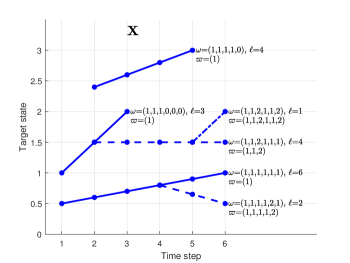
Figure 2: Illustration of a set of tree trajectories, with three tree trajectories, $\mathbf{X}=\left\{X_{1},X_{2},X_{3}\right\}$. The main branch (surviving mode) is represented as a continuous line. The dashed lines represent descendant branches from a main branch and the dashed dotted line a descendant branch from a secondary branch. At the end of each branch, it is written its genealogy variable $\omega$ up to time step 6, its ID $\varpi$ and its length $\ell$.

Let $t$ denote the time step when a target is born. At each of the following time steps $t+i-1$, $i>1$, this target and its descendants may generate new targets according to the spawning process. We refer to the time index $i$ as the $i$-th generation of the tree. The maximum number of generations in a tree is denoted by $\nu$. For example, if the current time step is $k$, $\nu=k-t+1$. Each spawning process from this target or its descendants generates a new branch.

Definition 1.

Given a branch that spawned at generation $i$ in a tree with at most $\nu$ generations, its genealogy $\omega=\left(\omega^{1},...,\omega^{\nu}\right)$ is defined as follows. Variable $\omega^{i}\in\left\{2,...,\varrho\right\}$ contains its spawning mode. For subsequent generations $j>i$, $\omega^{j}=1$ or $\omega^{j}=0$ if the branch is present or not present at generation $j$, respectively. For generations previous to the branch spawning, $j<i$, the branch inherits the genealogy variable $\omega^{j}$ of the parent branch. In particular, $\omega^{1}=1$ by convention indicating that the main branch of a tree is created by target birth.

The space of the genealogy variables is denoted by $I_{(\nu)}$ so that $\omega\in I_{(\nu)}$.

Definition 2.

A branch $B=\left(\omega,x^{1:\ell\left(\omega\right)}\right)$ consists of the genealogy variable $\omega$ and the sequence of states $x^{1:\ell\left(\omega\right)}=\left(x^{1},...,x^{\ell\left(\omega\right)}\right)$, where $x^{1}$ is the state at the time when the branch is spawned or born and $x^{2:\ell\left(\omega\right)}$ is the sequence of states at the following time steps. The length $\ell\left(\omega\right)$ of the branch is the number of time steps that the branch is present, which is a deterministic function of $\omega$, see Appendix A-A.

The single branch space in tree with at most $\nu$ generations is then $\mathbb{B}_{(\nu)}=\uplus_{\omega\in I_{(\nu)}}\left\{\omega\right\}\times\mathbb{R}^{\ell\left(\omega\right)\cdot n_{x}}$, where $\uplus$ denotes the union of disjoint sets [6]. That is, $\mathbb{B}_{(\nu)}$ contains all possible genealogy variables $\omega$, to which we append a sequence of target states of suitable length.

Definition 3.

A tree trajectory $X$ is a variable formed by the tree starting time $t$ and its set $\mathbf{B}$ of branches, such that $X=\left(t,\mathbf{B}\right)$ with $\mathbf{B}=\left\{B_{1},...,B_{n}\right\}$.

The space of single tree trajectories from time step 1 to $k$ is

$$\mathbb{T}_{(k)} =\uplus_{t=1}^{k}\left[\left\{t\right\}\times\mathcal{F}\left(\mathbb{B}_{(k-t+1)}\right)\right]$$ (1)

where $\mathcal{F}\left(\mathbb{B}_{(\nu)}\right)$ is the set of all finite subsets of $\mathbb{B}_{(\nu)}$. That is, the starting time $t$ belongs to $\{1,...,k\}$ and, for a given $t$, the branches have at most $\nu=k-t+1$ generations. Therefore, the set of branches belongs to $\mathcal{F}\left(\mathbb{B}_{(k-t+1)}\right)$. In addition, the genealogy variables of the branches in a tree require several constraints, described in Appendix A-B, so that an element of (1) corresponds to a tree. These constraints are ensured by a suitable birth and dynamic model, as in target labelling approaches, where label uniqueness is ensured probabilistically [22].

We should note that, according to the spawning process in Section II-A, the maximum number of branches in a tree trajectory with at most $\nu$ generations is

$$n_{max}\left(\nu\right)=\varrho^{\nu-1}.$$ (2)

Definition 4.

The ID $\varpi$ of a branch in a tree $X=\left(t,\mathbf{B}\right)$ is the branch genealogy variable $\omega$ up to the generation when the branch was spawned or born.

The ID $\varpi$ uniquely identifies each branch in a tree as there cannot be more than one branch in a tree with the same $\varpi$. Finally, a set of tree trajectories is denoted by $\mathbf{X}\in\mathcal{F}\left(\mathbb{T}_{(k)}\right)$. We illustrate the previous concepts via the following example.

Example 5.

We consider the set $\mathbf{X}$ of tree trajectories in Figure 2. The tree trajectory in the middle has start time $t=1$, $\nu=6$ and three branches, each with the genealogy variables, branch ID and lengths shown in the figure. The branch with $\omega=\left(1,1,2,1,1,2\right)$ was spawned at $\nu=6$, and has length 1. Its genealogy indicates that its parent branch spawned from the main branch at generation 3, as there is a 2 in the third entry in $\omega$. The tree trajectory at the top has start time $t=2$, $\nu=5$ and only has the main branch. The last entry in its genealogy is zero because it is not alive at time step 6.

II-C Integration

The space of single tree trajectories is locally compact, Hausdorff and second-countable (LCHS), see Appendix A-C. Then, we can use finite set statistics to define probabilistic models and integrals for sets of tree trajectories [6]. Given a real-valued function $\pi\left(\cdot\right)$ on $\mathbb{T}_{(k)}$, its single tree integral is

$$\int\pi\left(X\right)dX =\sum_{t=1}^{k}\int_{\mathbb{B}_{(k-t+1)}}\pi\left(t,\mathbf{B}\right)\delta\mathbf{B}$$ (3)

where we first sum over all possible start times, and the set integral is on the space of the set of branches with start time $t$ and maximum end time $k$. The set integral in (3) can also be written explicitly, see Appendix A-D. A function $\pi\left(\cdot\right)$ represents a density of a tree trajectory if $\pi\left(\cdot\right)\geq 0$ and it integrates to one. To be precise, this density should also ensure that the genealogy variables are unique and meet the genealogy constraints (parent/children relations), see Appendix A-B.

Given a function $\pi\left(\cdot\right)$ on $\mathcal{F}\left(\mathbb{T}_{(k)}\right)$, its set integral is [6]

$$\int\pi\left(\mathbf{X}\right)\delta\mathbf{X} =\sum_{n=0}^{\infty}\frac{1}{n!}\int\pi\left(\left\{X_{1},...,X_{n}\right\}\right)dX_{1:n}.$$ (4)

A function $\pi\left(\cdot\right)$ represents a density of a set of tree trajectories if $\pi\left(\cdot\right)\geq 0$, it integrates to one, and each tree meets the genealogy constraints. Equation (4) is a nested set integral, as each single tree trajectory integral has a set integral. Nested set integrals have been used for group targets [28, 29][6, Chap. 21].

II-C1 Set of branches integration

The single tree trajectory integral (3) requires the calculation of an integral over the set of branches with $\nu=k-t+1$ generations. In this section, we explain a way to perform this set integral that will be useful to derive the PMBM filter in Section IV.

The number of unique branch IDs, see Definition 4, in a set of branches $\mathbf{B}\in\mathcal{F}\left(\mathbb{B}_{(\nu)}\right)$ is $n_{max}\left(\nu\right)$, see (2). We arrange the branch IDs in a tree in lexicographical order (or any other order) to refer to each branch by an index $j=1,...,n_{max}\left(\nu\right)$. In a tree with $\nu$ generations, the $j$-th branch can have lengths from 1 to $\ell_{max}\left(\nu,j\right)$, which is used to denote the number of generations since its birth/spawning to $\nu$. Given $\nu$ and the branch length $l$, we can obtain the genealogy variable of the $j$-th branch, $\omega_{(\nu,j,l)}$.

We have that $\mathbb{B}_{(\nu)}=\uplus_{j=1}^{n_{max}\left(\nu\right)}\mathbb{B}_{(\nu,j)}$ where $\mathbb{B}_{(\nu,j)}$ is the space of branch $j$ in a tree with at most $\nu$ generations, which can be written as $\mathbb{B}_{(\nu,j)}=\uplus_{\ell=1}^{\ell_{max}\left(\nu,j\right)}\left\{\omega_{(\nu,j,l)}\right\}\times\mathbb{R}^{\ell\cdot n_{x}}$. That is, the single branch space $\mathbb{B}_{(\nu)}$ is the union of the spaces for each branch, which are disjoint sets as there cannot be two branches in a tree with the same genealogy variable. Then, we can decompose a given $\mathbf{B}$ as $\mathbf{B}^{1}\uplus...\uplus\mathbf{B}^{n_{max}\left(\nu\right)}=\mathbf{B}$, where $\mathbf{B}^{j}$ is the set representing the $j$-th branch, which meets $\left|\mathbf{B}^{j}\right|\leq 1$. Due to this decomposition of the single branch space into disjoint spaces, the set integral for a function $\pi\left(\cdot\right)$ on $\mathcal{F}\left(\mathbb{B}_{(\nu)}\right)$ can be written as [6, Sec. 3.5.3]

$$\int_{\mathbb{B}_{(\nu)}}\pi\left(\mathbf{B}\right)\delta\mathbf{B}$$

$$=\int...\int\pi\left(\mathbf{B}^{1}\uplus...\uplus\mathbf{B}^{n_{max}\left(\nu\right)}\right)\delta\mathbf{B}^{1}...\delta\mathbf{B}^{n_{max}\left(\nu\right)}.$$ (5)

In addition, if $\pi\left(\cdot\right)$ is a density on a set of branches, which implies $\pi\left(\mathbf{B}^{j}\right)=0$ for $\left|\mathbf{B}^{j}\right|>1$, the set integral on $\mathbf{B}^{j}$ is

$$\int\pi\left(\mathbf{B}^{j}\right)\delta\mathbf{B}^{j}$$

$$=\pi\left(\emptyset\right)+\sum_{\ell=1}^{\ell_{max}\left(\nu,j\right)}\int\pi\left(\left\{\left(\omega_{(\nu,j,\ell)},x^{1:\ell}\right)\right\}\right)dx^{1:\ell}.$$ (6)

That is, the set integral for the (uniquely identified) potential $j$-th branch goes through the hypotheses that it does not exist and that it exists with a length $\ell$, where $\ell$ takes values from 1 to its maximum possible length $\ell_{max}\left(\nu,j\right)$. The corresponding genealogy variable is $\omega_{(\nu,j,\ell)}$.

III Dynamic/measurement models for tree trajectories

In this section, we write the single tree trajectory dynamic and measurement models that arise from the single target models in Section II-A for computing the posterior density on the set of all tree trajectories.

III-A Dynamic model for all tree trajectories

A tree trajectory up to time step $k-1$ can be written as $X_{k-1}=\left(t_{k-1},\mathbf{B}_{k-1}\right)$, with the set of branches $\mathbf{B}_{k-1}=\mathbf{B}_{k-1}^{1}\uplus...\uplus\mathbf{B}_{k-1}^{n_{max}\left(k-t_{k-1}+1\right)}$, where $\mathbf{B}_{k-1}^{j}$ is the set representing the $j$-th branch, see Section II-C1. Each tree trajectory evolves independently of the rest and the dynamic model is characterised by the probability of survival of a tree trajectory $p^{S}(X_{k-1})$, single tree trajectory dynamic model $g\left(X_{k}|X_{k-1}\right)$ and PPP birth intensity $\lambda_{k}^{B}\left(X_{k}\right)$.

We consider the dynamic model for all tree trajectories, which implies that $p^{S}(X_{k-1})=1$, as all trajectories remain in the set of interest even if a tree trajectory is no longer present at the current time step [10, 30]. We denote the $m$-th branch spawned from $\mathbf{B}_{k-1}^{j}$ by $\mathbf{B}_{k}^{j,m}$, being $\mathbf{B}_{k}^{j,1}$ the surviving branch. As branches spawn independently, the single tree transition density is

$$g\left(t_{k},\uplus_{j,m}\mathbf{B}_{k}^{j,m}\left|t_{k-1},\mathbf{B}_{k-1}\right.\right)$$

$$=\delta_{t_{k-1}}\left[t_{k}\right]\prod_{j=1}^{n_{max}\left(k-t_{k-1}\right)}\prod_{m=1}^{\varrho}g_{m}\left(\mathbf{B}_{k}^{j,m}\left|t_{k-1},\mathbf{B}_{k-1}^{j}\right.\right)$$ (7)

where $\delta_{t}\left[\cdot\right]$ is a Kronecker delta at $t$. It should be noted that, in general, the density of a set that is the union of independent sets contains a convolution sum [6, 12]. In (7), there is no convolution sum as the unique identifiers in the genealogy variables provide the right association between the branches at time step $k$ and their parent at time step $k-1$.

If branch $\mathbf{B}_{k-1}^{j}=\emptyset,$ we have

$$g_{m}\left(\mathbf{B}_{k}^{j,m}\left|t_{k-1},\emptyset\right.\right) =\delta_{\emptyset}\left(\mathbf{B}_{k}^{j,m}\right)$$ (8)

for all $m$, where $\delta_{\emptyset}\left(\cdot\right)$ is a multi-object Dirac delta evaluated at $\emptyset$ [6]. That is, if branch $j$ does not exist, its descendants do not exist.

If branch $\mathbf{B}_{k-1}^{j}=\left\{\left(\omega,x^{1:\ell}\right)\right\}$ is not present at time step $k-1$ (the last element of $\omega$ is zero), then

$$g_{1}\left(\mathbf{B}_{k}^{j,1}\left|t_{k-1},\left\{\left(\omega,x^{1:\ell}\right)\right\}\right.\right)$$

$$=\begin{cases}\delta_{x^{1:\ell}}\left(y^{1:\ell}\right)&\mathbf{B}_{k}^{j,1}=\left\{\left(\left(\omega,0\right),y^{1:\ell}\right)\right\}\\ 0&\mathrm{otherwise}\end{cases}$$ (9)

where $\delta_{x}\left(\cdot\right)$ denotes a Dirac delta at $x$ and

$$g_{m}\left(\mathbf{B}_{k}^{j,m}\left|t_{k-1},\mathbf{B}_{k-1}^{j}\right.\right) =\delta_{\emptyset}\left(\mathbf{B}_{k}^{j,m}\right)$$ (10)

for $m>1$. That is, we append a zero entry to $\omega$ and keep the past trajectories information in the main branch, and there are no spawning branches.

If branch $\mathbf{B}_{k-1}^{j}=\left\{\left(\omega,x^{1:\ell}\right)\right\}$ is present at time step $k-1$ (the last element of $\omega$ is higher than zero), then, for $m=1$,

$$g_{1}\left(\mathbf{B}_{k}^{j,1}\left|t_{k-1},\left\{\left(\omega,x^{1:\ell}\right)\right\}\right.\right)$$

$$=\begin{cases}p_{1}^{S}\left(x^{\ell}\right)g_{1}\left(y^{\ell+1}|x^{\ell}\right)\\ \>\times\delta_{x^{1:\ell}}\left(y^{1:\ell}\right)&\mathbf{B}_{k}^{j,1}=\left\{\left(\left(\omega,1\right),y^{1:\ell+1}\right)\right\}\\ \left(1-p_{1}^{S}\left(x^{\ell}\right)\right)\delta_{x^{1:\ell}}\left(y^{1:\ell}\right)&\mathbf{B}_{k}^{j,1}=\left\{\left(\left(\omega,0\right),y^{1:\ell}\right)\right\}\\ 0&\mathrm{otherwise}\end{cases}$$ (11)

and, for $m>1$,

$$g_{m}\left(\mathbf{B}_{k}^{j,m}\left|t_{k-1},\left\{\left(\omega,x^{1:\ell}\right)\right\}\right.\right)$$

$$=\begin{cases}p_{m}^{S}\left(x^{\ell}\right)g_{m}\left(y|x^{\ell}\right)&\mathbf{B}_{k}^{j,m}=\left\{\left(\left(\omega,m\right),y\right)\right\}\\ 1-p_{m}^{S}\left(x^{\ell}\right)&\mathbf{B}_{k}^{j,m}=\emptyset\\ 0&\mathrm{otherwise}.\end{cases}$$ (12)

The main branch can either die (we append 0 to $\omega$) or survive (we append 1 to $\omega$ and the new state $y^{\ell+1}$ to previous branch state). Potential spawning branches may spawn or not. If they spawn they have a single state and we append its spawning mode $m$ to $\omega$.

Finally, the birth model for tree trajectories at time step $k$ is a PPP with intensity

$$\lambda_{k}^{B}\left(t,\mathbf{B}\right) =\begin{cases}\delta_{k}[t]\lambda^{B}\left(x\right)&\mathbf{B}=\left\{\left(1,x\right)\right\}\\ 0&\mathrm{otherwise}.\end{cases}$$ (13)

It should be noted that all new born trajectories have a single branch with genealogy variable $1$, as they only consist of the root node of the tree.

III-B Measurement model for tree trajectories

We can write the measurement model in Section II-A in terms of tree trajectories. To this end, we only need to write the density of the target generated measurements as a function of tree trajectories, the clutter model remains a PPP with intensity $\lambda^{C}\left(\cdot\right)$. Each tree trajectory $X\in\mathbf{X}_{k}$ generates a multi-Bernoulli set of measurements with density

$$f\left(\mathbf{z}|X\right) =\sum_{\mathbf{z}_{1}\uplus...\uplus\mathbf{z}_{\left|\tau_{k}\left(X\right)\right|}=\mathbf{z}}\prod_{i=1}^{\left|\tau_{k}\left(X\right)\right|}f\left(\mathbf{z}_{i}|x_{i}\right)$$ (14)

where $\tau_{k}\left(X\right)=\left\{x_{1},...,x_{\tau_{k}\left(X\right)}\right\}$ is the set of targets in $X$ at time step $k$, $f\left(\cdot|x\right)$ is the Bernoulli density of the measurement set generated by target $x$,

$$f\left(\mathbf{z}|x\right) =\begin{cases}1-p^{D}\left(x\right)&\mathbf{z}=\emptyset\\ p^{D}\left(x\right)l\left(z|x\right)&\mathbf{z}=\left\{z\right\}\\ 0&\left|\mathbf{z}\right|>1.\end{cases}$$

IV Tree Poisson multi-Bernoulli mixture density

In this section we explain the structure of the TrPMBM posterior. In Section IV-A, we explain the exact PMBM posterior for sets of all tree trajectories, with data associations at a tree level. In Section IV-B, we explain the proposed PMBM posterior with multi-Bernoulli branches in each Bernoulli tree and data associations at a branch level. Section IV-C explains the form of the single branch densities in the proposed PMBM filter.

IV-A Exact PMBM posterior for sets of tree trajectories

Tree trajectories are born independently following a PPP (13), and each tree trajectory moves independently of the rest following a Markovian process with single tree transition density (7) and probability of survival $p^{S}(X)=1$. The measurement model has a multi-Bernoulli form (14) with PPP clutter. These models correspond to a standard multi-object dynamic model [6] and a measurement model of the type in [27], being the underlying single object space the tree trajectory space.

Therefore, the posterior and predicted densities are PMBMs and are obtained via the recursion in [27] with the single tree trajectory space and integrals (see Section II) instead of the single target ones. That is, the density of the set of all tree trajectories at time step $k$ given the sequence of measurements up to time step $k^{\prime}=\left\{k,k-1\right\}$ is a PMBM of the form [27]

$$f_{k|k^{\prime}}\left(\mathbf{X}_{k}\right) =\sum_{\mathbf{Y}\uplus\mathbf{W}=\mathbf{X}_{k}}f_{k|k^{\prime}}^{\mathrm{p}}\left(\mathbf{Y}\right)f_{k|k^{\prime}}^{\mathrm{mbm}}\left(\mathbf{W}\right)$$ (15)

$$f_{k|k^{\prime}}^{\mathrm{p}}\left(\mathbf{X}_{k}\right) =e^{-\int\lambda_{k|k^{\prime}}\left(X\right)dX}\prod_{X\in\mathbf{X}_{k}}\lambda_{k|k^{\prime}}\left(X\right)$$ (16)

where $f_{k|k^{\prime}}^{\mathrm{p}}\left(\cdot\right)$ is the PPP density, which has intensity $\lambda_{k|k^{\prime}}\left(\cdot\right)$ and represents undetected tree trajectories, and $f_{k|k^{\prime}}^{\mathrm{mbm}}\left(\cdot\right)$ is an MBM representing potential tree trajectories detected at some point up to time step $k^{\prime}$. The summation in (15) is taken over all mutually disjoint (and possibly empty) sets $\mathbf{Y}$ and $\mathbf{W}$ whose union is $\mathbf{X}_{k}$. The MBM density is

$$f_{k|k^{\prime}}^{\mathrm{mbm}}\left(\mathbf{X}_{k}\right) =\sum_{a\in\mathcal{A}_{k|k^{\prime}}}w_{k|k^{\prime}}^{a}\sum_{\uplus_{i=1}^{n_{k|k^{\prime}}}\mathbf{X}_{k}^{i}=\mathbf{X}_{k}}\prod_{i=1}^{n_{k|k^{\prime}}}f_{k|k^{\prime}}^{i,a^{i}}\left(\mathbf{X}_{k}^{i}\right)$$ (17)

where $n_{k|k^{\prime}}$ is the number of potentially detected trees, $\mathcal{A}_{k|k^{\prime}}$ is the set of global tree hypotheses, $w_{k|k^{\prime}}^{a}$ is the weight of global tree hypothesis $a=\left(a^{1},...,a^{n_{k|k^{\prime}}}\right)$, which contains indices to local tree hypotheses for each potentially detected tree and $f_{k|k^{\prime}}^{i,a^{i}}\left(\cdot\right)$ is the Bernoulli density of the tree trajectory with local tree hypothesis $a^{i}.$ At each time step in each local hypothesis, we can associate more than one measurement to each Bernoulli tree, as each of its alive branches can generate one measurement, see (14). A global tree hypothesis $a$ indicates the measurements that are associated to each Bernoulli tree at each time step. All details regarding (15)-(17) can be found in [27, Sec. II.B].

IV-B Approximate PMBM posterior for sets of tree trajectories

A drawback of the above PMBM recursion is that it is difficult to handle the resulting Bernoulli tree densities because of the dependencies between branches that arise in the prediction step, and the global hypotheses defined at a tree level, i.e., associating measurements to Bernoulli trees instead of branches. To obtain a computationally efficient recursion (to be explained in Section V), with global hypotheses defined at a branch level, we introduce the following approximations:

• A1 The PPP represents alive branches without spawning.

• A2 Each Bernoulli tree trajectory has a deterministic start time.

• A3 After each prediction step, the set of branches in each Bernoulli tree trajectory is multi-Bernoulli.

As spawning is a low probability event, we use A1 to simplify implementation by discarding spawning events of potential targets we have never observed. The absence of spawning transforms the trees into single branch trees. A single branch tree can at most generate one measurement, and therefore, A1 implies that each measurement generates a new Bernoulli, similar to the PMBM recursion for point targets/trajectories [11, 10]. A newly created Bernoulli single branch tree may have multiple possible start times, which give rise to a mixture in each Bernoulli single tree density [10, Eq. (28)]. After the Bernoulli tree initialisation, all the mixture components in each Bernoulli tree are predicted and updated with the same equations. To simplify the filter implementation, we use A2 and take the most likely start time when a new Bernoulli is created. Approximation A2 is also used in the trajectory filters in [30].

Approximations A1 and A2 imply that Bernoulli tree densities have a single branch with a unique genealogy at the time step they are created. In addition, we know the genealogies of these potential branches for all Bernoulli trees. Approximation A3 is performed to simplify the filtering recursion by discarding the dependencies among branches within the same Bernoulli tree. It is performed at each prediction step using the KLD minimisation that will be explained in Section V-B.

IV-B1 Global branch hypotheses

In (17), global hypotheses are defined at a tree level, in which, at each step, we can associate more than one measurement to each Bernoulli tree. Using A1-A3, we can also define global hypotheses at a branch level (global branch hypotheses), in which we can associate at most one measurement to each potential branch in a Bernoulli tree. The number of potential branches in the $i$-th tree is denoted by $n_{k|k^{\prime}}^{i}$ (see (2)). Then, the total number of potential branches is $N_{k|k^{\prime}}=\sum_{i=1}^{n_{k|k^{\prime}}}n_{k|k^{\prime}}^{i}$. A local hypothesis for tree $i$ and branch $j$ is denoted by an index $\alpha^{i,j}\in\left\{1,...,h_{k|k^{\prime}}^{i,j}\right\}$, where $h_{k|k^{\prime}}^{i,j}$ is the number of local hypotheses.

A global branch hypothesis $\alpha$ is then a sequence of length $N_{k|k^{\prime}}$ containing the local hypothesis for each branch such that $\alpha=\left(\alpha^{i,j}\right)$ with $i=1,..,n_{k|k^{\prime}},j=1,..,n_{k|k^{\prime}}^{i}$. The set of global branch hypotheses is $\mathcal{D}_{k|k^{\prime}}$ and is defined as follows. We refer to measurement $z_{k}^{j}$ using the pair $\left(k,j\right)$ and the set of all such pairs $\left(k,j\right)$ up to (and including) time step $k$ is $\mathcal{M}_{k}$. Then, the set of measurement indices up to time step $k$ that correspond to local hypothesis $\alpha^{i,j}$ is $\mathcal{M}_{k}^{i,j,\alpha^{i,j}}\subseteq\mathcal{M}_{k}$, with at most one measurement per time step. The set $\mathcal{M}_{k}^{i,j,\alpha^{i,j}}$ is built recursively as will be explained in Section V-C. In a global hypothesis $\alpha\in\mathcal{D}_{k|k^{\prime}},$ all measurements must be associated to a local hypothesis, there can only be at most one measurement associated to a local hypothesis per time step and, there cannot be more than one local hypothesis associated with the same measurement.

IV-B2 Approximate MBM with global branch hypotheses

Under A1-A3 and using global branch hypotheses, the MBM density (17) can be written as

$$f_{k|k^{\prime}}^{\mathrm{mbm}}\left(\mathbf{X}_{k}\right) =\sum_{\alpha\in\mathcal{D}_{k|k^{\prime}}}w_{k|k^{\prime}}^{\alpha}\sum_{\uplus_{i=1}^{n_{k|k^{\prime}}}\mathbf{X}_{k}^{i}=\mathbf{X}_{k}}\prod_{i=1}^{n_{k|k^{\prime}}}f_{k|k^{\prime}}^{i,\alpha}\left(\mathbf{X}_{k}^{i}\right)$$ (18)

$$w_{k|k^{\prime}}^{\alpha} \propto\prod_{i=1}^{n_{k|k}}\prod_{j=1}^{n_{k|k^{\prime}}^{i}}w_{k|k^{\prime}}^{i,j,\alpha}$$ (19)

where $f_{k|k^{\prime}}^{i,\alpha}\left(\cdot\right)$ is the Bernoulli density of the $i$-th tree for a global branch hypothesis $\alpha$, and $w_{k|k^{\prime}}^{i,j,\alpha}$ is the weight of the $j$-th branch in the $i$-th tree in global branch hypothesis $\alpha$.

Due to A1-A3, $f_{k|k^{\prime}}^{i,\alpha}\left(\cdot\right)$ has a deterministic start time $\overline{t}^{i}$ and its branches are multi-Bernoulli, which means that $f_{k|k^{\prime}}^{i,\alpha}\left(\cdot\right)$ is characterised by $\overline{t}^{i}$ and $\left\{\left(r_{k|k^{\prime}}^{i,j,\alpha},p_{k|k^{\prime}}^{i,j,\alpha}\left(\cdot\right)\right)\right\}_{j=1}^{n_{k|k^{\prime}}^{i}}$ where $r_{k|k^{\prime}}^{i,j,\alpha}$ and $p_{k|k^{\prime}}^{i,j,\alpha}\left(\cdot\right)$ are the probability of existence and single branch density of the $j$-th branch of tree $i$ under global hypothesis $\alpha$, respectively. The set of branches in a tree thus follows a multi-Bernoulli distribution [6], in which the event with no branches is mapped to a no tree event, as a tree with no branches does not exist. With this mapping, we can write $f_{k|k^{\prime}}^{i,\alpha}\left(\cdot\right)$ as

$$f_{k|k^{\prime}}^{i,\alpha}\left(\mathbf{X}\right)$$

$$=\begin{cases}\delta_{\overline{t}^{i}}\left[t\right]\prod_{j=1}^{n_{k|k^{\prime}}^{i}}p_{k|k^{\prime}}^{i,j,\alpha}\left(\mathbf{B}^{j}\right)&\mathbf{X}=\left\{\left(t,\mathbf{B}\right)\right\},|\mathbf{B}|>0\\ \prod_{j=1}^{n_{k|k^{\prime}}^{i}}\left(1-r_{k|k^{\prime}}^{i,j,\alpha}\right)&\mathbf{X}=\emptyset\\ 0&\mathrm{otherwise}\end{cases}$$ (20)

$$p_{k|k^{\prime}}^{i,j,\alpha}\left(\mathbf{B}^{j}\right) =\begin{cases}r_{k|k^{\prime}}^{i,j,\alpha}p_{k|k^{\prime}}^{i,j,\alpha}\left(B\right)&\mathbf{B}^{j}=\left\{B\right\}\\ 1-r_{k|k^{\prime}}^{i,j,\alpha}&\mathbf{B}^{j}=\emptyset\\ 0&\mathrm{otherwise}\end{cases}$$ (21)

where $\overline{t}^{i}$ is the deterministic start time of the tree, $p_{k|k^{\prime}}^{i,j,\alpha}\left(\cdot\right)$ is the Bernoulli density of the $j$-th branch of tree $i$ under global hypothesis $\alpha$. Given a set of branches $\mathbf{B}$, $\mathbf{B}^{j}$ is the set for the $j$-th branch, which can have at most one element, see Section II-C1, and, as it is uniquely determined, there is no sum over the subsets of $\mathbf{B}$ in (20) (see the contrast w.r.t. (17), where there is a sum over the subsets of $\mathbf{X}_{k}$). It should be noted that $r_{k|k^{\prime}}^{i,j,\alpha}$, $p_{k|k^{\prime}}^{i,j,\alpha}\left(\cdot\right)$ and $w_{k|k^{\prime}}^{i,j,\alpha}$ only depend on element $\alpha^{i,j}$ of $\alpha$ but this is kept implicit for notational simplicity.

From (20), we note that the probability of existence and single tree density of $f_{k|k^{\prime}}^{i,\alpha}\left(\cdot\right)$ are

$$r_{k|k^{\prime}}^{i,\alpha} =1-\prod_{j=1}^{n_{k|k^{\prime}}^{i}}\left(1-r_{k|k^{\prime}}^{i,j,\alpha}\right).$$ (22)

$$p_{k|k^{\prime}}^{i,\alpha}\left(t,\mathbf{B}\right) =\frac{\delta_{\overline{t}^{i}}\left[t\right]\prod_{j=1}^{n_{k|k^{\prime}}^{i}}p_{k|k^{\prime}}^{i,j,\alpha}\left(\mathbf{B}^{j}\right)}{r_{k|k^{\prime}}^{i,\alpha}},\;|\mathbf{B}|>0.$$ (23)

In addition, A3 relaxes the genealogy constraints of the branches, see Section II-C, as sampled trees from (20) do not necessarily meet the constraints.

IV-C Single branch densities

In general, the single branch density $p_{k|k^{\prime}}^{i,j,\alpha}\left(\cdot\right)$ for the $i$-th Bernoulli tree, $j$-th branch and local hypothesis $\alpha^{i,j}$, see (21), can be written as

$$p_{k|k^{\prime}}^{i,j,\alpha}\left(\omega,x^{1:\ell}\right)$$

$$=\sum_{\kappa=\overline{t}^{i,j}}^{k}\beta_{k|k^{\prime}}^{i,j,\alpha}\left(\kappa\right)\delta_{\overline{\omega}_{k,\kappa}^{i,j}}\left[\omega\right]\delta_{\ell\left(\overline{\omega}_{k,\kappa}^{i,j}\right)}\left[\ell\right]p_{k|k^{\prime}}^{i,j,\alpha}\left(x^{1:\ell};\kappa\right)$$ (24)

where $\overline{t}^{i,j}$ is the start time of the branch, $\overline{\omega}_{k,\kappa}^{i,j}$ is the genealogy variable if the branch ends at time step $\kappa$, $\ell\left(\overline{\omega}_{k,\kappa}^{i,j}\right)$ is the length of the branch (see (71)), $\beta_{k|k^{\prime}}^{i,j,\alpha}\left(\kappa\right)$ is the probability that this branch ends at time step $\kappa$, and $p_{k|k^{\prime}}^{i,j,\alpha}\left(\cdot;\kappa\right)$ is the density of the states assuming the branch ends at time step $\kappa$. Note that $\beta_{k|k^{\prime}}^{i,j,\alpha}\left(\kappa\right)$ sums to one over $\kappa$.

Due to A1, the intensity of the PPP only considers a single, alive branch in each tree. Therefore,, $\lambda_{k|k^{\prime}}\left(X\right)$ is non-zero only for trees $X=\left(t,\left\{\omega,x^{1:\ell}\right\}\right)$ with its main branch alive

$$\lambda_{k|k^{\prime}}\left(t,\left\{\omega,x^{1:\ell}\right\}\right)$$

$$=\sum_{\overline{t}=1}^{k}\delta_{\overline{t}}\left[t\right]\delta_{1_{k-\overline{t}+1}}\left[\omega\right]\delta_{k-\overline{t}+1}\left[\ell\right]\lambda_{k|k^{\prime}}\left(x^{1:\ell};\overline{t}\right)$$ (25)

where $1_{\ell}$ is a sequence of length $\ell$ with all ones.

V TrPMBM filter recursion

This section explains the filtering recursion for the proposed TrPMBM filter, whose posterior density was explained in Section IV-B. The prediction step for the PPP is explained in Section V-A. We derive the Bernoulli tree prediction with independent branches via KLD minimisation in Section V-B. The PMBM update is explained in Section V-C.

V-A PPP prediction

Given $\lambda_{k-1|k-1}\left(\cdot\right)$ of the form (25), we apply the transition density of the surviving branch, as we use Approximation A1, and the PMBM prediction [11, 12, 10] to obtain

$$\lambda_{k|k-1}\left(t,\left\{\omega,x^{1:\ell}\right\}\right)=\lambda_{k}^{B}\left(t,\left\{\omega,x^{1:\ell}\right\}\right)$$

$$\qquad+\sum_{\overline{t}=1}^{k-1}\delta_{\overline{t}}\left[t\right]\delta_{1_{k-\overline{t}+1}}\left[\omega\right]\delta_{k-\overline{t}+1}\left[\ell\right]\lambda_{k|k-1}\left(x^{1:\ell};\overline{t}\right)$$ (26)

where $\lambda_{k}^{B}\left(\cdot\right)$ is given by (13) and

$$\lambda_{k|k-1}\left(x^{1:\ell+1};\overline{t}\right) =g_{1}\left(x^{\ell+1}|x^{\ell}\right)p_{1}^{S}\left(x^{\ell}\right)\lambda_{k-1|k-1}\left(x^{1:\ell};\overline{t}\right).$$

V-B Bernoulli tree prediction via KLD minimisation

In the prediction step, the number of Bernoulli trees does not change $n_{k|k-1}=n_{k-1|k-1}$ and we perform prediction for each tree, independently of the other trees. After the prediction, the set of branches in each tree is no longer multi-Bernoulli due to dependencies introduced by the spawning process. Therefore, we perform a KLD minimisation in each Bernoulli tree to approximate the set of branches as multi-Bernoulli, see A3.

Specifically, given $f_{k-1|k-1}^{i,\alpha}\left(\cdot\right)$ of the form (20), the true predicted Bernoulli $\widetilde{f}_{k|k-1}^{i,\alpha}\left(\cdot\right)$ is calculated with the transition density (7) and probability of survival, $p^{S}(X)=1$, to produce [11]

$$\widetilde{f}_{k|k-1}^{i,\alpha}\left(\mathbf{X}\right) =\begin{cases}\widetilde{r}_{k|k-1}^{i,\alpha}\delta_{\overline{t}^{i}}\left[t\right]\widetilde{p}_{k|k-1}^{i,\alpha}\left(\mathbf{B}\right)&\mathbf{X}=\left\{\left(t,\mathbf{B}\right)\right\}\\ 1-\widetilde{r}_{k|k-1}^{i,\alpha}&\mathbf{X}=\emptyset\end{cases}$$ (27)

where $\widetilde{r}_{k|k-1}^{i,\alpha}=r_{k-1|k-1}^{i,\alpha}$ and

$$\widetilde{p}_{k|k-1}^{i,\alpha}\left(\mathbf{B}_{k}\right)$$

$$=\int g\left(\mathbf{B}_{k}\left|X_{k-1}\right.\right)p_{k-1|k-1}^{i,\alpha}\left(X_{k-1}\right)dX_{k-1}$$ (28)

$$=\frac{1}{\widetilde{r}_{k|k-1}^{i,\alpha}}\int_{|\mathbf{B}_{k-1}|>0}\prod_{j=1}^{n_{k-1|k-1}^{i}}\left[\prod_{m=1}^{\varrho}g_{m}\left(\mathbf{B}_{k}^{j,m}\left|\overline{t}^{i},\mathbf{B}_{k-1}^{j}\right.\right)\right.$$

$$\quad\left.\times p_{k-1|k-1}^{i,j,\alpha}\left(\mathbf{B}_{k-1}^{j}\right)\right]\delta\mathbf{B}_{k-1}^{1:n_{k-1|k-1}^{i}}$$ (29)

where $p_{k-1|k-1}^{i,\alpha}\left(X_{k-1}\right)$ is given by (23), which requires $|\mathbf{B}_{k-1}|>0$. We should note that $\widetilde{p}_{k|k-1}^{i,\alpha}\left(\emptyset\right)=0$, as there is always at least one branch if the tree exists, and $g\left(\mathbf{B}_{k}\left|X_{k-1}\right.\right)$ corresponds to (7) without the tree start time.

Our aim is to find an approximation to $\widetilde{f}_{k|k-1}^{i,\alpha}\left(\cdot\right)$ with multi-Bernoulli branches of the form (20). We obtain this approximation via KLD minimisation resulting in the next propositions, which are proved in Appendix B and C, respectively.

Proposition 6.

Given the posterior tree Bernoulli density $f_{k-1|k-1}^{i,\alpha}\left(\cdot\right)$ of the form (20), the predicted tree Bernoulli density $f_{k|k-1}^{i,\alpha}\left(\cdot\right)$ of the form (20) that minimises the KLD $D\left(\widetilde{f}_{k|k-1}^{i,\alpha}||f_{k|k-1}^{i,\alpha}\right)$, where $\widetilde{f}_{k|k-1}^{i,\alpha}\left(\cdot\right)$ is the true predicted density, see (27), has a Bernoulli density for the $m$-th branch spawned from previous branch $j$ given by

$$p_{k|k-1}^{i,\left(j,m\right),\alpha}\left(\mathbf{B}_{k}^{j,m}\right) =\int g_{m}\left(\mathbf{B}_{k}^{j,m}\left|\overline{t}^{i},\mathbf{B}_{k-1}^{j}\right.\right)$$

$$\quad\times p_{k-1|k-1}^{i,j,\alpha}\left(\mathbf{B}_{k-1}^{j}\right)\delta\mathbf{B}_{k-1}^{j}.$$ (30)

Applying Proposition 6 to the single branch densities in (24), we obtain the following prediction step.

Proposition 7.

Given the Bernoulli tree density $f_{k-1|k-1}^{i,\alpha}\left(\cdot\right)$ of the form (20) with single branch density (24), the predicted Bernoulli tree density $f_{k|k-1}^{i,\alpha}\left(\cdot\right)$ of the form (20) with single branch density (24) that minimises the KLD $D\left(\widetilde{f}_{k|k-1}^{i,\alpha}||f_{k|k-1}^{i,\alpha}\right)$ has $n_{k|k-1}^{i}=\varrho\cdot n_{k-1|k-1}^{i}$ potential branches and the following parameters. For the surviving branch, $m=1$, the parameters are: $r_{k|k-1}^{i,j,\alpha}=r_{k-1|k-1}^{i,j,\alpha}$ and

$$\overline{\omega}_{k,\kappa}^{i,j} =\begin{cases}\left(\overline{\omega}_{k-1,k-1}^{i,j},1\right)&\kappa=k\\ \left(\overline{\omega}_{k,\kappa}^{i,j},0\right)&\kappa\in\{\overline{t}^{i,j},...,k-1\}\end{cases}$$ (31)

$$p_{k|k-1}^{i,j,\alpha}\left(x^{1:\ell};\kappa\right)$$

$$=\begin{cases}p_{k-1|k-1}^{i,j,\alpha}\left(x^{1:\ell};\kappa\right)&\kappa\in\left\{\overline{t}^{i,j},...,k-2\right\}\\ p_{k-1|k-1}^{i,j,\alpha}\left(x^{1:\ell};\kappa\right)\left(1-p_{1}^{S}\left(x^{\ell}\right)\right)&\kappa=k-1\\ p_{k-1|k-1}^{i,j,\alpha}\left(x^{1:\ell-1};k-1\right)\\ \quad\times p_{1}^{S}\left(x^{\ell-1}\right)g_{1}\left(x^{\ell}|x^{\ell-1}\right)&\kappa=k\end{cases}$$ (32)

$$\beta_{k|k-1}^{i,j,\alpha}(\kappa) =\begin{cases}\beta_{k-1|k-1}^{i,j,\alpha}(\kappa)&\kappa\in\left\{\overline{t}^{i,j},...,k-2\right\}\\ \left(1-p^{S}\right)\beta_{k-1|k-1}^{i,j,\alpha}(\kappa)&\kappa=k-1\\ p^{S}\beta_{k-1|k-1}^{i,j,\alpha}(k-1)&\kappa=k\end{cases}$$ (33)

where

$$p^{S}= \int p_{k-1|k-1}^{i,j,\alpha}\left(x^{\ell};k-1\right)p_{1}^{S}\left(x^{\ell}\right)dx^{\ell}$$ (34)

and $p_{k-1|k-1}^{i,j,\alpha}\left(x^{\ell};k-1\right)$ denotes the marginal density at the last state of the branch.

For the $m$-th branch spawning from previous branch $j$, the branch index is $j^{*}=j+(m-1)n_{k-1|k-1}^{i}$ and the parameters are: $h^{i,j^{*}}=h^{i,j}$, $\mathcal{M}_{k-1}^{i,j^{*},\alpha^{i,j^{*}}}=\emptyset$, $\beta_{k|k-1}^{i,j^{*},\alpha}(\kappa)=\delta_{k}[\kappa]$, $\overline{t}^{i,j^{*}}=k$, and

$$\overline{\omega}_{k,k}^{i,j^{*}} =\left(\overline{\omega}_{k-1,k-1}^{i,j},m\right)$$ (35)

$$p_{k|k-1}^{i,j^{*},\alpha}\left(y;k\right) =\frac{\int g_{m}\left(y|x^{\ell}\right)p_{m}^{S}\left(x^{\ell}\right)p_{k-1|k-1}^{i,j,\alpha}\left(x^{\ell};k-1\right)dx^{\ell}}{\left\langle p_{m}^{S}\left(x^{\ell}\right),p_{k-1|k-1}^{i,j,\alpha}\left(x^{\ell};k-1\right)\right\rangle}$$ (36)

$$r_{k|k-1}^{i,j^{*},\alpha} =r_{k-1|k-1}^{i,j,\alpha}\left\langle p_{m}^{S}\left(x^{\ell}\right),p_{k-1|k-1}^{i,j,\alpha}\left(x^{\ell};k-1\right)\right\rangle$$

$$\quad\times\beta_{k-1|k-1}^{i,j,\alpha}(k-1).$$ (37)

Due to the KLD minimisation, we propagate each branch in each local hypothesis independently of the rest. The surviving branch density contains information on past states of the branch, and its predicted density is similar to the standard trajectory case [30]. The spawned branches only have one state, corresponding to the current time step.

Proposition 6 makes the TrPMBM filter implementation considerably easier. If the spawning probability is zero, the TrPMBM filter computes the posterior density. Therefore, the posterior and the TrPMBM approximation are expected to be similar unless there is a high probability of a spawning event. Nevertheless, if the spawning event happens at a time step $k_{1}$, the difference between the posterior over the set of tree trajectories in a time interval $\left[k_{1}+\Delta k,k\right]$ and its approximation should vanish for a sufficiently large $\Delta k$, due to the forgetting property of Markov systems [31].

V-C Update

Given a global hypothesis, the branches in a predicted PMBM density with MBM of the form (18), are multi-Bernoulli. This implies that the updated density can be calculated similarly to the PMBM update on point targets and trajectories [11, 10], by performing the data associations for the Bernoulli branches. The resulting update is given in the following proposition.

Proposition 8.

Under Approximations A1-A3, given a predicted PMBM of the form (15), (16) and (18), the updated density with measurement set $\mathbf{z}_{k}=\left\{z_{k}^{1},...,z_{k}^{m_{k}}\right\}$ is a PMBM of the same form. The PPP intensity for undetected trees is

$$\lambda_{k|k}\left(t,\left\{\omega,x^{1:\ell}\right\}\right) =\left(1-p^{D}\left(x^{\ell}\right)\right)\lambda_{k|k-1}\left(t,\left\{\omega,x^{1:\ell}\right\}\right)$$ (38)

where $\lambda_{k|k-1}\left(\cdot\right)$ is given by (25).

The number of updated Bernoulli tree components is $n_{k|k}=n_{k|k-1}+m_{k}$. For each previous Bernoulli branch $j\in\left\{1,...,n_{k|k-1}^{i}\right\}$ in a previous Bernoulli tree $i\in\left\{1,...,n_{k|k-1}\right\}$, the update creates $\left(m_{k}+1\right)$ new local hypotheses corresponding to a missed detection and an update with one of the received measurements, which implies $h_{k|k}^{i,j}=h_{k|k-1}^{i,j}\left(m_{k}+1\right)$. For missed detection hypotheses, $\alpha^{i,j}\in\left\{1,...,h_{k|k-1}^{i,j}\right\},$ the parameters are $\mathcal{M}_{k}^{i,j,\alpha^{i,j}}=\mathcal{M}_{k-1}^{i,j,\alpha^{i,j}}$

$$w_{k|k}^{i,j,\alpha} =w_{k|k-1}^{i,j,\alpha}\left(1-r_{k|k-1}^{i,j,\alpha}\beta_{k|k-1}^{i,j,\alpha}\left(k\right)p_{k}^{D,i,j,\alpha}\right)$$ (39)

$$r_{k|k}^{i,j,\alpha} =\frac{r_{k|k-1}^{i,j,\alpha}\left(1-\beta_{k|k-1}^{i,j,\alpha}\left(k\right)p_{k}^{D,i,j,\alpha}\right)}{1-r_{k|k-1}^{i,j,\alpha}\beta_{k|k-1}^{i,j,\alpha}\left(k\right)p_{k}^{D,i,j,\alpha}}$$ (40)

$$\beta_{k|k}^{i,j,\alpha}\left(\kappa\right) \propto\begin{cases}\beta_{k|k-1}^{i,j,\alpha}\left(\kappa\right)&\overline{t}^{i,j}\leq\kappa<k\\ \left(1-p_{k}^{D,i,j,\alpha}\right)\beta_{k|k-1}^{i,j,\alpha}\left(k\right)&\kappa=k\end{cases}$$ (41)

$$p_{k|k}^{i,j,\alpha}\left(x^{1:\ell};\kappa\right) =\begin{cases}p_{k|k-1}^{i,j,\alpha}\left(x^{1:\ell};\kappa\right)&\overline{t}^{i,j}\leq\kappa<k\\ \frac{p_{D}\left(x^{\ell}\right)p_{k|k-1}^{i,j,\alpha}\left(x^{1:\ell};k\right)}{p_{k}^{D,i,j,\alpha}}&\kappa=k\end{cases}$$ (42)

where

$$p_{k}^{D,i,j,\alpha} =\left\langle p^{D},p_{k|k-1}^{i,j,\alpha}\left(\cdot;k\right)\right\rangle$$

$$=\int p^{D}\left(x^{\ell}\right)p_{k|k-1}^{i,j,\alpha}\left(x^{\ell};k\right)dx^{\ell}.$$ (43)

For a previous Bernoulli branch $j\in\left\{1,...,n_{k|k-1}^{i}\right\}$ in Bernoulli tree $i\in\left\{1,...,n_{k|k-1}\right\}$ with $\widetilde{\alpha}^{i,j}\in\left\{1,...,h_{k|k-1}^{i,j}\right\}$, the new local hypothesis generated by measurement $z_{k}^{m}$ has $\alpha^{i,j}=\widetilde{\alpha}^{i,j}+h_{k|k-1}^{i,j}m$, $r_{k|k}^{i,j,\alpha}=1$, and

$$\mathcal{M}_{k}^{i,j,\alpha^{i,j}} =\mathcal{M}_{k-1}^{i,j,\widetilde{\alpha}^{i,j}}\cup\left\{\left(k,m\right)\right\}$$ (44)

$$w_{k|k}^{i,j,\alpha} =w_{k|k-1}^{i,j,\widetilde{\alpha}}r_{k|k-1}^{i,j,\widetilde{\alpha}}\beta_{k|k-1}^{i,j,\widetilde{\alpha}}\left(k\right)l\left(z_{k}^{m}\right)$$ (45)

$$\beta_{k|k}^{i,j,\alpha}\left(\kappa\right) =\begin{cases}0&\overline{t}^{i,j}\leq\kappa<k\\ 1&\kappa=k\end{cases}$$ (46)

$$p_{k|k}^{i,j,\alpha}\left(x^{1:\ell};k\right) \propto l\left(z_{k}^{m}|x^{\ell}\right)p^{D}\left(x^{\ell}\right)p_{k|k-1}^{i,j,\widetilde{\alpha}}\left(x^{1:\ell};k\right)$$ (47)

$$l\left(z_{k}^{m}\right) =\left\langle l\left(z_{k}^{m}|\cdot\right)p^{D}\left(\cdot\right),p_{k|k-1}^{i,j,\widetilde{\alpha}}\left(\cdot;k\right)\right\rangle.$$ (48)

Finally, the Bernoulli tree initiated by measurement $z_{k}^{m}$, whose index is $i=n_{k|k-1}+m$, has one branch ($j=1$), $h_{k|k}^{i,1}=2$ local hypotheses, one with a non-existent Bernoulli

$$\mathcal{M}_{k}^{i,1,1}=\emptyset,\;w_{k|k}^{i,1,1}=1,\;r_{k|k}^{i,1,1}=0$$ (49)

and the other with $\mathcal{M}_{k}^{i,1,2}=\left\{z_{k}^{m}\right\}$, and

$$w_{k|k}^{i,1,2} =\lambda^{C}\left(z_{k}^{m}\right)+\sum_{\overline{t}=1}^{k}\left\langle l\left(z_{k}^{m}|\cdot\right)p^{D},\lambda_{k|k-1}\left(\cdot;\overline{t}\right)\right\rangle$$ (50)

$$r_{k|k}^{i,1,2} =\frac{\sum_{\overline{t}=1}^{k}\left\langle l\left(z_{k}^{m}|\cdot\right)p^{D},\lambda_{k|k-1}\left(\cdot;\overline{t}\right)\right\rangle}{w_{k|k}^{i,1,2}}$$ (51)

$$\overline{t}^{i} =\underset{\overline{t}}{\arg\max}\left\langle l\left(z_{k}^{m}|\cdot\right)p^{D},\lambda_{k|k-1}\left(\cdot;\overline{t}\right)\right\rangle$$ (52)

$$p_{k|k}^{i,1,2}\left(\omega,x^{1:\ell}\right) \propto l\left(z|x^{\ell}\right)p^{D}\left(x^{\ell}\right)\lambda_{k|k-1}\left(\overline{t}^{i},\left\{\omega,x^{1:\ell}\right\}\right).$$ (53)

As the predicted PPP is a mixture with different start times, see (25), the newly created Bernoulli trees may have multiple start times. To have a tree with deterministic start time and simplify filter implementation, see A2 and (23), we take the most likely start time in (52) to obtain the density (53).

We would like to remark that, if targets are born according to a multi-Bernoulli birth model instead of Poisson birth model, the posterior is a multi-Bernoulli mixture (MBM), which is a PMBM with PPP intensity set to zero. The MBM posterior can be computed with the same prediction and update as in the PMBM filter (with PPP intensity equal to zero) adding the Bernoulli components of new born targets in the prediction step [12, 13].

VI Gaussian TrPMBM filter recursion

In this section, we explain the Gaussian implementation of the TrPMBM filter for the linear/Gaussian model:

• $l\left(\cdot|x\right)=\mathcal{N}\left(\cdot;Hx,R\right)$ and $p^{D}\left(x\right)=p^{D}$.

• $g_{m}\left(\cdot|x\right)=\mathcal{N}\left(\cdot;F_{m}x+d_{m},Q_{m}\right)$ and $p_{m}^{S}\left(x\right)=p_{m}^{S}$ for $m\in\{1,...,\varrho\}$.

• $\lambda_{k}^{B}\left(x\right)=\sum_{q=1}^{n_{k}^{b}}w_{k}^{b,q}\mathcal{N}\left(x;\overline{x}_{k}^{b,q},P_{k}^{b,q}\right)$.

If we set $\varrho=1$, which implies there is no spawning, the Gaussian TrPMBM filter implementation becomes the Gaussian trajectory PMBM filter implementation for all trajectories in [30], which also uses Approximations A1 and A2. The single branch Gaussian densities are explained in Section IV-C. The prediction step is explained in Sections VI-B and VI-C. The update is addressed in Section VI-D. Practical aspects and estimation are explained in Sections VI-E and VI-F.

VI-A Single branch Gaussian densities

We define a Gaussian density on a single branch space as

$$\mathcal{N}\left(\omega,x^{1:\ell};\overline{\omega},\overline{x},P\right) =\begin{cases}\mathcal{N}\left(x^{1:\ell};\overline{x},P\right)&\omega=\overline{\omega},\ell=\ell\left(\overline{\omega}\right)\\ 0&\mathrm{otherwise}\end{cases}$$ (54)

where $\overline{\omega}$ is the genealogy, $\ell\left(\overline{\omega}\right)$ is the length of the branch (number of states in the branch), see (71), $\overline{x}$ is the $n_{x}\ell\left(\overline{\omega}\right)\times 1$ mean vector and $P$ the $n_{x}\ell\left(\overline{\omega}\right)\times n_{x}\ell\left(\overline{\omega}\right)$ covariance.

Then, the single branch density (24) on a branch $B=\left(\omega,x^{1:\ell}\right)$ can be written as

$$p_{k|k^{\prime}}^{i,j,\alpha}\left(B\right) =\sum_{\kappa=\overline{t}^{i,j}}^{k}\beta_{k|k^{\prime}}^{i,j,\alpha}\left(\kappa\right)$$

$$\quad\times\mathcal{N}\left(B;\overline{\omega}_{k,\kappa}^{i,j},\overline{x}_{k|k^{\prime}}^{i,j,\alpha}\left(\kappa\right),P_{k|k^{\prime}}^{i,j,\alpha}\left(\kappa\right)\right)$$ (55)

where $\overline{\omega}_{k,\kappa}^{i,j}$, $\overline{x}_{k|k^{\prime}}^{i,j,\alpha}\left(\kappa\right)$ and $P_{k|k^{\prime}}^{i,j,\alpha}\left(\kappa\right)$ are the genealogy, mean and covariance of the $j$-th branch in the $i$-th tree, with end time $\kappa$. The PPP intensity (25) is

$$\lambda_{k|k^{\prime}}\left(t,\left\{B\right\}\right) =\sum_{q=1}^{n_{k|k^{\prime}}^{p}}w_{k|k^{\prime}}^{p,q}\delta_{\overline{t}_{k|k^{\prime}}^{p,q}}[t]$$

$$\quad\times\mathcal{N}\left(B;1_{k-\overline{t}_{k|k^{\prime}}^{p,q}+1},\overline{x}_{k|k^{\prime}}^{p,q},P_{k|k^{\prime}}^{p,q}\right)$$ (56)

where $n_{k|k^{\prime}}^{p}$ is the number of PPP terms, $\overline{t}_{k|k^{\prime}}^{p,q}$, $w_{k|k^{\prime}}^{p,q}$, $\overline{x}_{k|k^{\prime}}^{p,q}$ and $P_{k|k^{\prime}}^{p,q}$ are the start time, weight, mean and covariance of the $q$-th term.

It should be noted that the single branch Gaussian (54) is analogous to the single trajectory Gaussian for filters based on sets of trajectories [30, Eq. (40)], with the aditional information of the genealogy variable $\overline{\omega}$. A similar relation holds for the single branch density (55) and PPP intensity (56), see Eq. (64) and (43) in [30].

VI-B Gaussian PPP prediction

Given the birth intensity for targets, see Section VI, the birth intensity for trees can be written as

$$\lambda_{k}^{B}\left(t,\left\{B\right\}\right) =\sum_{q=1}^{n_{k}^{b}}w_{k}^{b,q}\delta_{k}[t]\mathcal{N}\left(B;1,\overline{x}_{k}^{b,q},P_{k}^{b,q}\right)$$

where the tree start time is $k$ and the genealogy variable for new born branches is 1, see (13).

Let us consider the posterior PPP intensity at time step $k-1$ is of the form (56). The predicted PPP intensity is obtained using (26) and the Kalman filter prediction step [32] to obtain

$$\lambda_{k|k-1}\left(t,\left\{B\right\}\right)$$

$$=\lambda_{k}^{B}\left(t,\left\{B\right\}\right)+p_{1}^{S}\sum_{q=1}^{n_{k-1|k-1}^{p}}w_{k-1|k-1}^{p,q}$$

$$\times\delta_{\overline{t}_{k-1|k-1}^{p,q}}[t]\mathcal{N}\left(B;1_{k-\overline{t}_{k-1|k-1}^{p,q}+1},\overline{x}_{k|k-1}^{p,q},P_{k|k-1}^{p,q}\right)$$ (57)

where

$$\overline{x}_{k|k-1}^{p,q} =\left[\left(\overline{x}_{k-1|k-1}^{p,q}\right)^{T},\left(\overline{F}_{1}\overline{x}_{k-1|k-1}^{p,q}+d_{1}\right)^{T}\right]^{T}$$ (58)

$$P_{k|k-1}^{p,q} =\left[\begin{array}[]{cc}P_{k-1|k-1}^{p,q}&P_{k-1|k-1}^{p,q}\overline{F}_{1}^{T}\\ \overline{F}_{1}P_{k-1|k-1}^{p,q}&\overline{F}_{1}P_{k-1|k-1}^{p,q}\overline{F}_{1}^{T}+Q_{1}\end{array}\right]$$ (61)

$$\overline{F}_{1} =\left[0_{1,k-\overline{t}_{k-1|k-1}^{p,q}-1},1\right]\otimes F_{1}$$ (62)

where $0_{n,m}$ is a zero matrix of size $n\times m$.

VI-C Gaussian Bernoulli tree prediction

The prediction for each Bernoulli tree is given by Proposition 7. We consider that a single branch density in the PMBM posterior at time $k-1$ is of the form (55). Then, for the linear Gaussian models, the predicted density for the main branch is

$$p_{k|k-1}^{i,j,\alpha}\left(B\right) =\sum_{\kappa=\overline{t}^{i,j}}^{k}\beta_{k|k-1}^{i,j,\alpha}\left(\kappa\right)$$

$$\times\mathcal{N}\left(B;\overline{\omega}_{k,\kappa}^{i,j},\overline{x}_{k|k-1}^{i,j,\alpha}\left(\kappa\right),P_{k|k-1}^{i,j,\alpha}\left(\kappa\right)\right)$$ (63)

where $\overline{\omega}_{k,\kappa}^{i,j}$ is given by (31), $\overline{x}_{k|k-1}^{i,j,\alpha}\left(\kappa\right)=\overline{x}_{k-1|k-1}^{i,j,\alpha}\left(\kappa\right)$ and $P_{k|k-1}^{i,j,\alpha}\left(\kappa\right)=P_{k-1|k-1}^{i,j,\alpha}\left(\kappa\right)$ for $\kappa<k$, and $\overline{x}_{k|k-1}^{i,j,\alpha}\left(k\right)$ and $P_{k|k-1}^{i,j,\alpha}\left(k\right)$ are obtained using (58) and (61) with $\overline{x}_{k-1|k-1}^{i,j,\alpha}\left(k-1\right)$ and $P_{k-1|k-1}^{i,j,\alpha}\left(k-1\right)$ instead of $\overline{x}_{k-1|k-1}^{p,q}$ and $P_{k-1|k-1}^{p,q}$. We also have that

$$\beta_{k|k-1}^{i,j,\alpha}\left(\kappa\right) =\begin{cases}\beta_{k-1|k-1}^{i,j,\alpha}(\kappa)&\kappa\in\left\{\overline{t}^{i,j},...,k-2\right\}\\ \left(1-p_{1}^{S}\right)\beta_{k-1|k-1}^{i,j,\alpha}(\kappa)&\kappa=k-1\\ p_{1}^{S}\beta_{k-1|k-1}^{i,j,\alpha}(k-1)&\kappa=k.\end{cases}$$ (64)

For the $m$-th branch spawning from previous branch $j$, we obtain $\overline{t}_{k}^{i,j^{*}}=k$, $\beta_{k|k-1}^{i,j^{*},\alpha}\left(k\right)=1$, $\overline{\omega}_{k,\kappa}^{i,j^{*}}$ given by (35), and

$$\overline{x}_{k|k-1}^{i,j^{*},\alpha}\left(k\right) =\overline{F}_{m}\overline{x}_{k-1|k-1}^{i,j,\alpha}\left(k-1\right)+d_{m}$$ (65)

$$P_{k|k-1}^{i,j^{*},\alpha}\left(k\right) =\overline{F}_{m}P_{k-1|k-1}^{i,j,\alpha}\left(k-1\right)F_{m}^{T}+Q_{m}$$ (66)

$$r_{k|k-1}^{i,j^{*},\alpha} =r_{k-1|k-1}^{i,j,\alpha}p_{m}^{S}\beta_{k-1|k-1}^{i,j,\alpha}(k-1)$$ (67)

where $j^{*}$ is the index of the spawning branch, $\overline{F}_{m}$ is obtained analogously to (62), but using $F_{m}$ and $\ell(\overline{\omega}_{k-1|k-1}^{i,j})$ instead of $F_{1}$ and $k-\overline{t}_{k-1|k-1}^{p,q}+1$.

VI-D Gaussian implementation update

Due to the multi-Bernoulli branches in (18) and the form of the single branch densities (55) and PPP intensity (56), the TrPMBM update in Proposition 8 with Gaussian models is equivalent to the Gaussian TPMBM update used in [30], so we do not provide further details. We would like to remark that, in the Gaussian implementation, the Bernoulli density of a new branch, see (52) and (53), uses the tree start time, mean and covariance of the component with highest weight. The analogous equations for trajectories are Eq. (60)-(63) in [30].

VI-E Practical aspects

To deal with covariance matrices of increasingly long branches, we use the $L$-scan approximation [33, 30]. This approximation sets the covariance matrices of the PPP and Bernoulli branches as block diagonal

$$P_{k|k} \approx\mathrm{diag}\left(\tilde{P}_{k|k}^{\overline{t}},\tilde{P}_{k|k}^{\overline{t}+1},...,\tilde{P}_{k|k}^{k-L},\tilde{P}_{k|k}^{k-L+1:k}\right)$$ (68)

where $\tilde{P}_{k|k}^{k-L+1:k}\in\mathbb{R}^{L\cdot n_{x}\times L\cdot n_{x}}$ is the joint covariance of the last $L$ time steps, $\tilde{P}_{k|k}^{k}\in\mathbb{R}^{n_{x}\times n_{x}}$ is the covariance of the branch state at time step $k$, and $\overline{t}$ is the branch start time. That is, branch states before the last $L$ time steps are approximated as independent, and are not updated with new measurements. The rationale behind this approximation is that, due to the Markovian nature, a current measurement does not have much effect on past branch states sufficiently far in the past. The window size $L$ acts as a trade-off between accuracy and computational complexity. The higher $L$ becomes, the more accurate the approximation ($L=k$ being the exact filter), and the higher the computational burden.

As global and local hypotheses grow unboundedly with time, we apply PMBM pruning techniques [34, Sec. V.D]. In PMBM pruning, global hypothesis weights, PPP weights and probability of existences that are sufficiently low are set to zero, and the corresponding global hypotheses, PPP and Bernoulli components can be removed from the posterior. In the proposed Gaussian TrPMBM implementation, we perform pruning analogously to the pruning of the PMBM posterior on the set of all trajectories in [30, Sec. V.C]. In particular, in the update, we use ellipsoidal gating [35] to discard unlikely measurement to Bernoulli associations. In addition, for each previous global hypothesis, we use Murty’s algorithm, in combination with the Hungarian algorithm, to choose the $k=\left\lceil N_{h}\cdot w_{k|k-1}^{\alpha}\right\rceil$ new global hypotheses with highest weights [36, 12]. After the update, we discard global hypotheses whose weight is below a threshold $\Gamma_{mbm}$ and only keep the $N_{h}$ global hypotheses with highest weights. We also eliminate Bernoulli components whose existence is below a threshold $\Gamma_{b}$ and the PPP components whose weight is below $\Gamma_{p}$. If $\beta_{k|k}^{i,j,\alpha}\left(k\right)<\Gamma_{a}$, we set $\beta_{k|k}^{i,j,\alpha}\left(k\right)=0$, which implies that the branch is no longer updated or predicted, but it is still a component of the posterior.

Finally, we would like to point out that the Gaussian implementation, presented for linear/Gaussian models, can be generalised to non-linear/non-Gaussian models. To do so, one can approximate $p^{D}\left(\cdot\right)$ and $p^{S}\left(\cdot\right)$ as constants with their value at the current state mean and use a non-linear Kalman filter [37, 32, 38, 39] for the single branch prediction and update steps, see (32), (36), (47) and (53). It is also possible to use importance Gaussian quadrature/sigma-points [40] to improve the normalising constant approximation in the update, see (48) and (52). More information on these approaches in the context of multi-object filtering can be found in [41]. Another possibility is to implement the TrPMBM recursion via particle filtering [42].

VI-F Estimation

We can apply several estimators to a PMBM posterior (15) to estimate the set $\mathbf{\hat{X}}_{k}$ of tree trajectories [12, Sec. VI]. We adapt Estimator 1 in [12, Sec. VI] for tree trajectories. We first take the global hypothesis $\alpha_{*}$ with highest weight, and then, we obtain the most likely end time for the $j$-th branch of the $i$-th tree

$$\kappa_{*}^{i,j} =\underset{\kappa}{\arg\max}\,\beta_{k|k}^{i,j,\alpha_{*}}\left(\kappa\right).$$ (69)

The estimated set of branches for the $i$-th tree is $\mathbf{\hat{B}}_{k}^{i}=\left\{\left(\overline{\omega}_{k,\kappa_{*}^{i,j}}^{i,j},\overline{x}_{k|k}^{i,j,\alpha_{*}}\left(\kappa_{*}^{i,j}\right)\right):r_{k|k}^{i,j,\alpha_{*}}>\Gamma_{d}\right\}$, which reports the genealogy variables and means with most likely length of the Bernoulli branches whose existence probability is greater than $\Gamma_{d}$. Then, the estimated set of trees is $\mathbf{\hat{X}}_{k}=\left\{\left(\overline{t}^{i},\mathbf{\hat{B}}_{k}^{i}\right):\mathbf{\hat{B}}_{k}^{i}\neq\emptyset\right\}$, which includes the trees that have at least one estimated branch. A pseudocode of the Gaussian TrPMBM filter is provided in Algorithm 1.

Algorithm 1 Gaussian TrPMBM filter pseudocode

- Set $\lambda_{0|0}\left(\cdot\right)=0$, $n_{0|0}=0$.

for $k=1$ to final time step  do

     - Prediction:

      $\circ\,$Predict the PPP, see Sec. VI-B.

      $\circ\,$Predict the Bernoulli branches, see Sec. VI-C.

      $\circ\,$Apply $L$-scan to all covariance matrices, see (68).

     - Update:

      $\circ\,$Update single branch hypotheses with ellipsoidal gating, see Prop. 8.

      $\circ\,$Go through previous global hypotheses, obtaining best ranked updated global hypotheses with Murty’s algorithm, see Sec. VI-E.

     - Estimate the set of all tree trajectories, see Sec. VI-F.

     - Prune PPP components, global hypotheses, and Bernoulli branches, see Sec. VI-E.

end for

VII Simulations

In this section, we evaluate the proposed TrPMBM and TrMBM filters. These filters have been implemented with the parameters (see Section VI-E): $N_{h}=100$, $\Gamma_{mbm}=10^{-4}$, $\Gamma_{p}=10^{-4}$, $\Gamma_{b}=10^{-4},$ $\Gamma_{a}=10^{-4}$, gating threshold 15, $\Gamma_{d}=0.4,$ and $L\in\{1,5\}$. We have also implemented the PMBM filter with spawning (S-PMBM) in [21], which uses recycling [43] to add the information on spawned targets into the PPP. In addition, we have implemented two filters that do not take into account spawning: the PMBM [11, 12] and the trajectory PMBM (TPMBM) filter [10, 30]. The TPMBM provides information on the trajectory of each branch, but not on the genealogy. The PMBM and S-PMBM filter do not provide genealogy information either and estimate the trajectory of each branch sequentially by linking estimates with the same auxiliary variable [30]. All filters have been implemented with the same parameters as the TrPMBM filter (where applicable). We have also tested the GLMB filter with spawning, with a maximum of 1000 global hypotheses [22]. All the units in this section are in the international system.

The single target state is $x=\left[p_{x},\dot{p}_{x},p_{y},\dot{p}_{y}\right]^{T}$, which contains position and velocity in a two-dimensional plane. Targets move with $p_{1}^{S}=0.99$ and the nearly constant velocity model with $d_{1}$ a zero vector,

$$F_{1}=I_{2}\otimes\left(\begin{array}[]{cc}1&\tau\\ 0&1\end{array}\right),\quad Q_{1}=qI_{2}\otimes\left(\begin{array}[]{cc}\tau^{3}/3&\tau^{2}/2\\ \tau^{2}/2&\tau\end{array}\right),$$

where $\tau=1$ and $q=0.01$. Targets can spawn with two modes ($\varrho=3$) perpendicular to the current target direction, one in each direction. A unit vector perpendicular to the target direction is $u_{\perp}=\left[-\dot{p}_{y},0,\dot{p}_{x},0\right]^{T}/\sqrt{\dot{p}_{x}^{2}+\dot{p}_{y}^{2}}$. Then, $d_{2}=5\cdot u_{\perp}$, $d_{3}=-5\cdot u_{\perp}$, and

$$F_{2}=\left(\begin{array}[]{cccc}1&0&0&-\tau\\ 0&0&0&-1\\ 0&\tau&1&0\\ 0&1&0&0\end{array}\right),\quad F_{3}=\left(\begin{array}[]{cccc}1&0&0&\tau\\ 0&0&0&1\\ 0&-\tau&1&0\\ 0&-1&0&0\end{array}\right)$$

also, $Q_{1}=Q_{2}=Q_{3}$. The spawning probabilities of the two modes are $p_{2}^{S}=p_{3}^{S}=0.01$. In the prediction step, we approximate the value of $u_{\perp}$ at the predicted mean to perform the prediction for the linear/Gaussian models, see Section VI-E.

We measure target position with

$$H=\left(\begin{array}[]{cccc}1&0&0&0\\ 0&0&1&0\end{array}\right),\quad R=\sigma^{2}I_{2},$$

where $\sigma^{2}=4$, and $p_{D}=0.9$. The clutter intensity is $\lambda^{C}\left(z\right)=\overline{\lambda}^{C}u_{A}\left(z\right)$ where $u_{A}\left(z\right)$ is a uniform density in $A=\left[0,600\right]\times\left[0,400\right]$ and $\overline{\lambda}^{C}=10$. The birth intensity is characterised by $n_{k}^{b}=1$, $\overline{x}_{k}^{b,1}=\left[300,3,170,1\right]^{T}$ and $P_{k}^{b,1}=\mathrm{diag}\left(\left[160^{2},1,100^{2},1\right]\right)$, and $w_{k}^{b,1}=0.08$. The TrMBM and GLMB filters use multi-Bernoulli birth with one Bernoulli with existence probability $0.08$ and the same mean and covariance matrix to match the PHD of the PPP birth model [6].

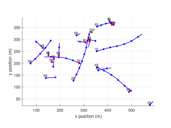
Figure 3: Scenario of the simulations. Each tree trajectory is shown in blue. Target positions every 10 time steps are marked with a blue circle. A spawning event is marked with a red square. The numbers next to a target birth or spawning event indicate the corresponding time step. There are 9 trees and 23 branches.

The ground truth set of tree trajectories with $N_{s}=100$ time steps has been obtained sampling from the dynamic model and is shown in Figure 3. We evaluate the filters via Monte Carlo simulation with $N_{mc}=100$ runs. To computes the estimation error, we take the estimated set $\mathbf{\hat{X}}_{k}$ of trees and discard tree and genealogy information to obtain an estimated set of trajectories $\mathbf{\hat{T}}_{k}$, where we have one trajectory per each branch [8]. We measure the error between $\mathbf{\hat{T}}_{k}$ and the ground truth set $\mathbf{T}_{k}$ of trajectories only considering the positional elements. Error is computed with the linear programming metric $d\left(\cdot,\cdot\right)$ for sets of trajectories in [44] with parameters $p=2$, $c=10$ and $\gamma=1$, see Appendix D for a review of its main characteristics. That is, the root mean square (RMS) error at a given time step $k$, normalised by $k$ as in [30], is

$$d\left(k\right) =\sqrt{\frac{1}{N_{mc}k}\sum_{i=1}^{N_{mc}}d^{2}\left(\mathbf{T}_{k},\mathbf{\hat{T}}_{k}^{i}\right)},$$ (70)

where $\mathbf{\hat{T}}_{k}^{i}$ is the estimated set of trajectories at time $k$ in the $i$-th Monte Carlo run.

We show the RMS trajectory metric error as a function of time in Figure 4. We can see that the best performing filter is the TrPMBM ($L=5$) followed by the TrMBM ($L=5$) and the TPMBM ($L=5$). This is reasonable as the TrPMBM filter approximates the posterior density over the set of tree trajectories, which contains full information on the trees. Behind these filters, we can find these filters implemented with $L=1$, for which we expect lower performance as they do not perform smoothing while filtering.

The filters with lowest performance are the GLMB, the PMBM and the S-PMBM. These filters estimate trajectories by linking target state estimates with the same label or auxiliary variable. This approach is inherently sub-optimal as it does not perform estimation of the trajectories directly from a posterior density. The GLMB filter has the lowest performance as it requires a higher number of global hypotheses than a PMBM filter to represent the same information [12, Sec. IV][30, App.D]. The reason is that GLMB has global hypotheses with deterministic target existence, while PMBM global hypotheses have probabilistic target existence and undetected targets are efficiently represented in the PMBM via a PPP. This results in an exponential increase in the number of global hypotheses in the GLMB filter compared to the PMBM filter [12, Sec. IV], and usually implies lower performance and higher computational burden. The S-PMBM has better performance than the PMBM filter as it accounts for target spawning.

Figure 4: RMS trajectory metric error to estimate all the branches at each time step.

The decomposition of the RMS trajectory metric error into localisation, missed target, false target and track switch costs is shown in Figure 5. The main difference between TrPMBM and TrMBM is in the lower missed target cost of the TrPMBM. This is a typical difference between PMBM and MBM filters [45], due to the measurement-driven track initialisation in PMBM filtering. Increasing $L$ lowers the localisation error of the trajectory and tree trajectory filters. The reason is that with a higher value of $L$, we can improve the estimation of past states of each trajectory, improving localisation error. In this setting, increasing $L$ does not affect the rest of the costs. TPMBM filters have quite similar performance to TrPMBM up to time step 52, then performance worsens, mainly due to localisation and missed target costs. This is expected as the first target spawning is at time step 53, so trajectory and tree trajectory filters work analogously up to this time step, and then TrPMBM works better. GLMB, PMBM and S-PMBM have higher costs, and the main difference in performance w.r.t. the other filters is due to a higher number of false and missed targets, and they also experience more track switches. For example, these sequential track estimators may leave gaps in the estimated trajectories, even though trajectories do have gaps according to the dynamic model. Tree or trajectory filters do not leave gaps in estimated trajectories, as the estimation is performed directly from the trajectory/tree posterior.

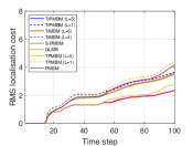
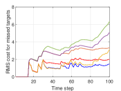
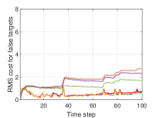
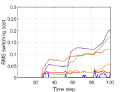
Figure 5: RMS trajectory metric decomposition into localisation cost, missed target cost, false target cost and track switching cost at each time step.

The computational times of one Monte Carlo run of the filters on an Intel core i5 laptop are provided in Table II. The GLMB filter has the highest computational burden, due to its higher number of global hypotheses, followed by TrPMBM and TrMBM. The TPMBM filter is faster than TrPMBM and TrMBM filters, as TPMBM does not take into account target spawning or tree information. The filters with $L=1$ are faster than those with $L=5$, due to the faster single branch updates. As expected, the PMBM filter is the fastest filter, as it does not account for spawning and only keeps information on the current set of targets.

Table II: Average computational times in seconds of the filters

$L$	TrPMBM	TrMBM	TPMBM	S-PMBM	PMBM	GLMB
$1$	9.8	6.0	2.6	2.5	1.5	25.9
$5$	10.3	6.2	2.6

VIII Conclusions

In this paper, we have shown that we can obtain all information on the trajectories of multiple spawning targets and their genealogies by computing the posterior density on the set of all tree trajectories. We have also shown that this posterior density is a PMBM, and we have proposed a computationally efficient PMBM filter with independent branches, derived via Kullback-Leibler divergence minimisation after the prediction.

It is possible to extend the TrPMBM recursion to extended targets, and coexisting point and extended targets [34, 27] by using the corresponding density for the set of measurements generated by a single target. Further work includes the design of other types of multi-target tracking algorithms for sets of tree trajectories.

Supplementary material: “Tracking multiple spawning targets using Poisson multi-Bernoulli mixtures on sets of tree trajectories”

Appendix A

This appendix provides more details on trees and branches.

A-A Length of a branch

The mathematical formula that defines the length of a branch with genealogy $\omega=\left(\omega^{1},...,\omega^{\nu}\right)$ is

$$\ell\left(\omega\right)=e\left(\omega\right)-i\left(\omega\right)+1$$ (71)

where

$$e\left(\omega\right)=\begin{cases}\nu&\omega^{i^{\prime}}\neq 0,\forall i^{\prime}\\ \min\left(i^{\prime}:\omega^{i^{\prime}}=0\right)-1&\mathrm{otherwise}\end{cases}$$ (72)

$$i\left(\omega\right)=\begin{cases}1&\omega^{i^{\prime}}\leq 1,\forall i^{\prime}\\ \max\left(i^{\prime}:\omega^{i^{\prime}}>1\right)&\mathrm{otherwise}.\end{cases}$$ (73)

We would like to remark that $i\left(\omega\right)$ is the generation when the branch was spawned or born, and $e\left(\omega\right)$ is the last generation when the branch is present.

A-B Genealogy constraints

The genealogy variables in a tree trajectory are subject to two constraints: uniqueness and consistent offspring. Let us consider the tree trajectory

$$X =\left(t,\left\{\left(\omega_{1},x_{1}^{1:\ell_{1}}\right),...,\left(\omega_{n},x_{n}^{1:\ell_{n}}\right)\right\}\right)$$ (74)

with $\omega_{i}=\left(\omega_{i}^{1},...,\omega_{i}^{\nu}\right)$. Given $\omega_{i}$, its unique identifier $\varpi_{i}$, see Definition 4, is

$$\varpi_{i} =\left(\omega_{i}^{1},...,\omega_{i}^{i\left(\omega_{i}\right)}\right)$$ (75)

where $i\left(\omega_{i}\right)$ is given by (73). Uniqueness means that there cannot be more than one branch with a unique identifier: $\nexists\,i,j$, $i\neq j$, such that $\varpi_{i}=\varpi_{j}$. In addition, a tree must have a main branch, with unique identifier 1, which also implies $n>0$.

The property of consistent offspring is as follows. For each $i$ and $k$ such that $\omega_{i}^{k}>1$ (i.e., there is a spawning event in branch $i$ at generation $k$), there is a $j\neq i$ such that $\omega_{j}^{1:k-1}=\omega_{i}^{1:k-1}$ and $\omega_{j}^{k}\in\left\{0,1\right\}$. That is, if there is branch $i$ with spawning at generation $k$, there must be a parent branch $j$, which has the same genealogy up to generation $k-1$, and then either it survives (with its main mode) $\omega_{j}^{k}=1$ or it terminates $\omega_{j}^{k}=0$ at generation $k$.

A-C Tree trajectory space is LCHS

In this appendix, we explain why the space of single tree trajectories is locally compact, Hausdorff and second-countable (LCHS) [6, 8, 13]. The space of a branch $\mathbb{B}_{(\nu)}=\uplus_{\omega\in I_{(\nu)}}\left\{\omega\right\}\times\mathbb{R}^{\ell\left(\omega\right)\cdot n_{x}}$ is LCHS. The proof is similar to the proof that the single trajectory space is LCHS [8, App. A]. The space $\mathcal{F}\left(\mathbb{B}_{(k-t+1)}\right)$ is compact, Hausdorff and second-countable, which implies that it is LCHS, see [46, Thm. 1-2-1]. Finally, as $\mathbb{T}_{(k)}$ is the disjoint union of LCHS spaces, we can also follow [8, App. A] to show that $\mathbb{T}_{(k)}$ is LCHS.

A-D Explicit single tree integral

By expanding the set integral inside the single tree integral in (3), we can write (3) as [6]

$$\int\pi\left(X\right)dX$$

$$=\sum_{t=1}^{k}\sum_{n=0}^{n_{max}\left(k-t+1\right)}\frac{1}{n!}\sum_{\omega_{1:n}\in I_{(k-t+1)}^{n}}\int$$

$$\quad\pi\left(t,\left\{\left(\omega_{1},x_{1}^{1:\ell_{1}}\right),...,\left(\omega_{n},x_{n}^{1:\ell_{n}}\right)\right\}\right)d\left(x_{1}^{1:\ell_{1}}...x_{n}^{1:\ell_{n}}\right)$$ (76)

where the branch length $\ell_{i}$ is determined by $\omega_{i}$, i.e., $\ell_{i}=\ell\left(\omega_{i}\right)$, see Appendix A-A, $n_{max}\left(\cdot\right)$ is given by (2), and $I_{(\nu)}^{n}$ denotes the $n$-th Cartesian power of $I_{(\nu)}$.

Appendix B

In this appendix we prove Proposition 6. We use $\mathrm{z}$ to denote constants whose values do not affect the minimisation. The products with indices $j$ and $m$ go through $j\in\left\{1,...,n_{k-1|k-1}^{i}\right\}$ and $m\in\left\{1,...,\varrho\right\}$. The KLD is [6]

$$D\left(\widetilde{f}_{k|k-1}^{i,\alpha}||f_{k|k-1}^{i,\alpha}\right)$$

$$=\int\widetilde{f}_{k|k-1}^{i,\alpha}\left(\mathbf{X}_{k}\right)\log\frac{\widetilde{f}_{k|k-1}^{i,\alpha}\left(\mathbf{X}_{k}\right)}{f_{k|k-1}^{i,\alpha}\left(\mathbf{X}_{k}\right)}\delta\mathbf{X}_{k}$$

$$=\mathrm{z}-\prod_{j}\left(1-r_{k-1|k-1}^{i,j,\alpha}\right)\log\prod_{j,m}\left(1-r_{k|k-1}^{i,\left(j,m\right),\alpha}\right)$$

$$-\sum_{t}\int\widetilde{f}_{k|k-1}^{i,\alpha}\left(\left\{\left(t,\mathbf{B}_{k}\right)\right\}\right)\log f_{k|k-1}^{i,\alpha}\left(\left\{\left(t,\mathbf{B}_{k}\right)\right\}\right)\delta\mathbf{B}_{k}$$

$$=\mathrm{z}-\prod_{j}\left(1-r_{k-1|k-1}^{i,j,\alpha}\right)\log\prod_{j,m}\left(1-r_{k|k-1}^{i,\left(j,m\right),\alpha}\right)$$

$$-\widetilde{r}_{k|k-1}^{i,\alpha}\int_{|\mathbf{B}_{k}|>0}\widetilde{p}_{k|k-1}^{i,\alpha}\left(\mathbf{B}_{k}\right)$$

$$\times\log\left[\prod_{j,m}p_{k|k-1}^{i,\left(j,m\right),\alpha}\left(\mathbf{B}_{k}^{j,m}\right)\right]\delta\mathbf{B}_{k}$$

$$=\mathrm{z}-\prod_{j}\left(1-r_{k-1|k-1}^{i,j,\alpha}\right)\log\left[\prod_{j,m}\left(1-r_{k|k-1}^{i,\left(j,m\right),\alpha}\right)\right]$$

$$-\int_{|\mathbf{B}_{k}|>0}\int_{|\mathbf{B}_{k-1}|>0}\prod_{j,m}g_{m}\left(\mathbf{B}_{k}^{j,m}\left|\overline{t}^{i},\mathbf{B}_{k-1}^{j}\right.\right)$$

$$\times p_{k-1|k-1}^{i,j,\alpha}\left(\mathbf{B}_{k-1}^{j}\right)\delta\mathbf{B}_{k-1}^{1:n_{k-1|k-1}^{i}}$$

$$\times\log\left[\prod_{j,m}p_{k|k-1}^{i,\left(j,m\right),\alpha}\left(\mathbf{B}_{k}^{j,m}\right)\right]\delta\mathbf{B}_{k}.$$ (77)

According to the dynamic model and the posterior at time $k-1$, the following equalities hold

$$\widetilde{f}_{k|k-1}^{i,\alpha}\left(\emptyset\right) =\prod_{j}\left(1-r_{k-1|k-1}^{i,j,\alpha}\right)$$

$$=\prod_{j,m}g_{m}\left(\emptyset\left|\overline{t}^{i},\emptyset\right.\right)p_{k-1|k-1}^{i,j,\alpha}\left(\emptyset\right).$$ (78)

That is, the predicted tree is empty if there are no branches at time step $k-1$, which implies no branches at time step $k$. Therefore, we can remove the domain of integration $|\mathbf{B}_{k}|>0$ and $|\mathbf{B}_{k-1}|>0$ by incorporating the previous term in (77) into the integral to obtain

$$D\left(\widetilde{f}_{k|k-1}^{i,\alpha}||f_{k|k-1}^{i,\alpha}\right)$$

$$=\mathrm{z}-\int\int\prod_{j,m}g_{m}\left(\mathbf{B}_{k}^{j,m}\left|\overline{t}^{i},\mathbf{B}_{k-1}^{j}\right.\right)p_{k-1|k-1}^{i,j,\alpha}\left(\mathbf{B}_{k-1}^{j}\right)$$

$$\times\delta\mathbf{B}_{k-1}^{1:n_{k-1|k-1}^{i}}\sum_{j,m}\log\left[p_{k|k-1}^{i,\left(j,m\right),\alpha}\left(\mathbf{B}_{k}^{j,m}\right)\right]\delta\mathbf{B}_{k}$$

$$=\mathrm{z}-\sum_{j,m}\int\int g_{m}\left(\mathbf{B}_{k}^{j,m}\left|\overline{t}^{i},\mathbf{B}_{k-1}^{j}\right.\right)p_{k-1|k-1}^{i,j,\alpha}\left(\mathbf{B}_{k-1}^{j}\right)$$

$$\times\delta\mathbf{B}_{k-1}^{j}\log\left[p_{k|k-1}^{i,\left(j,m\right),\alpha}\left(\mathbf{B}_{k}^{\left(j,m\right)}\right)\right]\delta\mathbf{B}_{k}^{j,m}.$$

By standard KLD minimisation we obtain (30), which proves Proposition 6.

Appendix C

In this appendix we prove Proposition 7. We evaluate (30) at $\mathbf{B}_{k}^{j,m}=\left\{B\right\}$

$$p_{k|k-1}^{i,\left(j,m\right),\alpha}\left(\left\{B\right\}\right) =\int g_{m}\left(\left\{B\right\}\left|\overline{t}^{i},\left\{B^{\prime}\right\}\right.\right)p_{k-1|k-1}^{i,j,\alpha}\left(B^{\prime}\right)dB^{\prime}.$$ (79)

We proceed to analyse the cases $m=1$ and $m>1$.

C-A Case $m=1$

The probability of existence of $p_{k|k-1}^{i,(j,1),\alpha}\left(\cdot\right)$ in (79) is

$$r_{k|k-1}^{i,(j,1),\alpha} =\int p_{k|k-1}^{i,(j,1),\alpha}\left(\left\{B\right\}\right)dB$$

$$=r_{k-1|k-1}^{i,j,\alpha}$$ (80)

where we have used that $g_{1}\left(\cdot|\cdot\right)$ in (11) does not change cardinality. The predicted single branch density is

$$p_{k|k-1}^{i,(j,1),\alpha}\left(B\right) =\frac{p_{k|k-1}^{i,(j,1),\alpha}\left(\left\{B\right\}\right)}{r_{k|k-1}^{i,(j,1),\alpha}}$$ (81)

$$=\int g_{1}\left(\left\{B\right\}\left|t_{k-1},\left\{B^{\prime}\right\}\right.\right)p_{k-1|k-1}^{i,j,\alpha}\left(B^{\prime}\right)dB^{\prime}.$$ (82)

We calculate (82) using (6), (9), (11), and (24) to obtain

$$p_{k|k-1}^{i,(j,1),\alpha}\left(B\right)$$

$$=\sum_{\kappa=\overline{t}^{i,j}}^{k-1}\int g_{1}\left(\left\{B\right\}\left|t_{k-1},\left\{\left(\omega,y^{1:\ell}\right)\right\}\right.\right)\beta_{k-1|k-1}^{i,j,\alpha}\left(\kappa\right)$$

$$\,\times\delta_{\overline{\omega}_{k-1,\kappa}^{i,j}}\left[\omega\right]\delta_{\ell(\overline{\omega}_{k-1,\kappa}^{i,j})}\left[\ell\right]p_{k-1|k-1}^{i,j,\alpha}\left(y^{1:\ell};\kappa\right)dy^{1:\ell}.$$ (83)

If we evaluate (83) at $B=\left(\left(\overline{\omega}_{k-1,\kappa}^{i,j},0\right),x^{1:\ell(\overline{\omega}_{k-1,\kappa}^{i,j})}\right)$ with $\kappa<k-1$, we obtain the first entries in (32) and (33). If we evaluate (83) at $B=\left(\left(\overline{\omega}_{k-1,\kappa}^{i,j},0\right),x^{1:\ell(\overline{\omega}_{k-1,\kappa}^{i,j})}\right)$ with $\kappa=k-1$, we obtain the second entries in (32) and (33). If we evaluate (83) at $B=\left(\left(\overline{\omega}_{k-1,\kappa}^{i,j},1\right),x^{1:\ell(\overline{\omega}_{k-1,\kappa}^{i,j})+1}\right)$, we obtain the third entries in (32) and (33). If we evaluate (83) at any other $B$, the output is zero. This finishes the proof of (32) and (33).

C-B Case $m>1$

The probability of existence of $p_{k|k-1}^{i,(j,m),\alpha}\left(\cdot\right)$, $m>1$, in (79) is

$$r_{k|k-1}^{i,(j,m),\alpha} =\int\widetilde{p}_{k|k-1}^{i,(j,m),\alpha}\left(\left\{B\right\}\right)dB$$

$$=\int\int g_{m}\left(\left\{B\right\}\left|t_{k-1},\left\{B^{\prime}\right\}\right.\right)$$

$$\,\times r_{k-1|k-1}^{i,j,\alpha}p_{k-1|k-1}^{i,j,\alpha}\left(B^{\prime}\right)dB^{\prime}dB.$$ (84)

As $g_{m}\left(\cdot|\cdot\right)$ requires an existing branch at time step $k-1$ and only depends on the last state of the parent branch, we can use (24) to obtain

$$r_{k|k-1}^{i,(j,m),\alpha} =r_{k-1|k-1}^{i,j,\alpha}\beta_{k-1|k-1}^{i,j,\alpha}\left(k-1\right)$$

$$\>\times\left\langle p_{m}^{S}\left(x^{\ell}\right),p_{k-1|k-1}^{i,j,\alpha}\left(x^{\ell};k-1\right)\right\rangle.$$ (85)

The predicted single branch density evaluated at branch $\left(\left(\overline{\omega}_{k-1,k-1}^{i,j},m\right),y\right)$ is

$$p_{k|k-1}^{i,(j,m),\alpha}\left(\left(\overline{\omega}_{k-1,k-1}^{i,j},m\right),y\right)$$

$$=\frac{p_{k|k-1}^{i,(j,m),\alpha}\left(\left\{\left(\overline{\omega}_{k-1,k-1}^{i,j},m\right),y\right\}\right)}{r_{k|k-1}^{i,(j,m),\alpha}}$$ (86)

$$=\frac{1}{r_{k|k-1}^{i,(j,m),\alpha}}\int g_{m}\left(\left\{\left(\overline{\omega}_{k-1,k-1}^{i,j},m\right),y\right\}\left|t_{k-1},\left\{B^{\prime}\right\}\right.\right)$$

$$\>\times r_{k-1|k-1}^{i,j,\alpha}p_{k-1|k-1}^{i,j,\alpha}\left(B^{\prime}\right)dB^{\prime}$$

$$=\frac{1}{\left\langle p_{m}^{S}\left(x\right),p_{k-1|k-1}^{i,j,\alpha}\left(x;k-1\right)\right\rangle}\int p_{m}^{S}\left(x^{\ell}\right)$$

$$\>\times g_{m}\left(y|x^{\ell}\right)p_{k-1|k-1}^{i,j,\alpha}\left(x^{\ell};k-1\right)dx^{\ell}$$ (87)

where $p_{k-1|k-1}^{i,j,\alpha}\left(x^{\ell};k-1\right)$ denotes the marginal distribution of $p_{k-1|k-1}^{i,j,\alpha}\left(\cdot;k-1\right)$ at the last time step of the branch. Eq. (87) corresponds to a density of the form (24) with one mixture component, $\beta_{k|k-1}^{i,(j,m),1}(k)=1$ and $p_{k|k-1}^{i,(j,m),\alpha}\left(y;k\right)$ given by (36), completing the proof of Proposition 7.

Appendix D

For completeness, this appendix reviews the main aspects of the linear programming (LP) metric for sets of trajectories. Full details are provided in [44].

D-A Preliminary concepts

We consider two sets of trajectories $\mathbf{T}^{x}=\left\{T_{1}^{x},...,T_{n_{x}}^{x}\right\}$ and $\mathbf{T}^{y}=\left\{T_{1}^{y},...,T_{n_{y}}^{y}\right\}$, with trajectories up to a time step $k_{\mathrm{max}}$. Let $\mathbf{x}_{i}^{k}$ and $\mathbf{y}_{j}^{k}$ denote the sets of targets at time step $k$ corresponding to trajectories $T_{i}^{x}$ and $T_{j}^{y}$. It is met that $|\mathbf{x}_{i}^{k}|\leq 1$ and $|\mathbf{y}_{j}^{k}|\leq 1$, i.e., a trajectory $T_{i}^{x}$ may not exist at time step $k$ ($\mathbf{x}_{i}^{k}=\emptyset$) or contain a single target ($\mathbf{x}_{i}^{k}=\left\{x\right\}$).

Let $d_{G}\left(\cdot,\cdot\right)$ denote the generalised optimal subpattern assignment (GOSPA) metric (with its parameter $\alpha=2$) for sets of targets [47]. For sets with at most one target, such as $\mathbf{x}_{i}^{k}$ and $\mathbf{y}_{j}^{k}$, the GOSPA metric becomes

$$d_{G}\left(\mathbf{x}_{i}^{k},\mathbf{y}_{j}^{k}\right) =\begin{cases}\min\left(c,d_{b}\left(x,y\right)\right)&\mathbf{x}_{i}^{k}=\left\{x\right\},\mathbf{y}_{j}^{k}=\left\{y\right\}\\ 0&\mathbf{x}_{i}^{k}=\mathbf{y}_{j}^{k}=\emptyset\\ \frac{c}{2^{1/p}}&\mathrm{otherwise}\end{cases}$$ (88)

where $d_{b}\left(\cdot,\cdot\right)$ is a base distance for single targets, $p$ is a scalar such that $1\leq p<\infty$ and parameter $c>0$ represents the maximum localisation error to regard a target $x$ as being properly detected by an estimate $y$.

We define an $(n_{x}+1)\times(n_{y}+1)$ matrix $D_{\mathbf{T}^{x},\mathbf{T}^{y}}^{k}$ whose $(i,j)$ element is

$$D_{\mathbf{T}^{x},\mathbf{T}^{y}}^{k}(i,j) =d_{G}\left(\mathbf{x}_{i}^{k},\mathbf{y}_{j}^{k}\right)^{p}$$ (89)

with $\mathbf{x}_{n_{x}+1}^{k}=\emptyset$ and $\mathbf{y}_{n_{y}+1}^{k}=\emptyset$. That is, $D_{\mathbf{T}^{x},\mathbf{T}^{y}}^{k}$ contains all possible GOSPA errors (to the $p$-th power) between all possible associations between $\mathbf{x}_{i}^{k}$ and $\mathbf{y}_{j}^{k}$.

In the trajectory metric, at each time step, we assign trajectories in $\mathbf{T}^{x}$ to trajectories in $\mathbf{T}^{y}$, or leave the trajectories unassigned. We represent these assignments using a binary matrix $W^{k}$ that satisfies the following properties:

$$\sum_{i=1}^{n_{x}+1}W^{k}(i,j) =1,\ j=1,\ldots,n_{y}$$ (90)

$$\sum_{j=1}^{n_{y}+1}W^{k}(i,j) =1,\ i=1,\ldots,n_{x}$$ (91)

$$W^{k}(n_{x}+1,n_{y}+1) =0,$$ (92)

$$W^{k}(i,j) \in\{0,1\},\forall\ i,j$$ (93)

where $W^{k}(i,j)$ is the element in the row $i$ and column $j$ of matrix $W^{k}$. We have $W^{k}(i,j)=1$ if $\mathbf{x}_{i}^{k}$ is associated to $\mathbf{y}_{j}^{k}$, $W^{k}(i,n_{y}+1)=1$ if $\mathbf{x}_{i}^{k}$ is unassigned, and $W^{k}(n_{x}+1,j)=1$ if $\mathbf{y}_{j}^{k}$ is unassigned.

D-B LP trajectory metric

To enable a fast computation, in the LP trajectory metric, we consider soft assignments between the sets of targets at each time step. That is, we consider a matrix $W^{k}\in\mathcal{\overline{W}}_{\mathbf{T}_{x},\mathbf{\mathbf{T}_{y}}}$ that meets (90)-(92) and $W^{k}(i,j)\in\left[0,1\right]$.

Definition 9.

For $1\leq p<\infty$, cut-off $c>0$, switching penalty $\gamma>0$, base metric $d_{b}\left(\cdot,\cdot\right)$, the LP metric for sets of trajectories $\mathbf{T}^{x}$ and $\mathbf{T}^{y}$ is

$$d\left(\mathbf{T}^{x},\mathbf{T}^{y}\right) =\min_{\begin{subarray}{c}W^{k}\in\mathcal{\overline{W}}_{\mathbf{T}^{x},\mathbf{T}^{y}}\\ k=1,\ldots,k_{\mathrm{max}}\end{subarray}}\Bigg{(}\sum_{k=1}^{k_{\mathrm{max}}}\mathrm{tr}\big{[}\big{(}D_{\mathbf{T}^{x},\mathbf{T}^{y}}^{k}\big{)}^{T}W^{k}\big{]}$$

$$\quad+\frac{\gamma^{p}}{2}\sum_{k=1}^{k_{\mathrm{max}}-1}\sum_{i=1}^{n_{x}}\sum_{j=1}^{n_{y}}|W^{k}(i,j)-W^{k+1}(i,j)|\Bigg{)}^{\frac{1}{p}}.$$ (94)

Namely, the LP trajectory metric uses the optimal soft-assignment between trajectories in $\mathbf{T}^{x}$ and $\mathbf{T}^{y}$ at each time step. The first term in (94) considers the costs for localisation errors, missed and false targets. The second term in (94) is the track switching cost. All details on the metric decomposition into these costs are provided in [44, Sec. IV.C].

References

• [1] S. Blackman and R. Popoli, Design and Analysis of Modern Tracking Systems.   Artech House, 1999.
• [2] L. Gao, G. Battistelli, L. Chisci, and P. Wei, “Distributed joint sensor registration and multitarget tracking via sensor network,” IEEE Transactions on Aerospace and Electronic Systems, vol. 56, no. 2, pp. 1301–1317, 2020.
• [3] Q. Chen and A. Tsukada, “Detection-by-tracking boosted online 3D multi-object tracking,” in IEEE Intelligent Vehicles Symposium, 2019, pp. 295–301.
• [4] N. Chenouard et al., “Objective comparison of particle tracking methods,” Nature methods, vol. 11, no. 3, pp. 281–290.
• [5] K. E. G. Magnusson, J. Jaldén, P. M. Gilbert, and H. M. Blau, “Global linking of cell tracks using the Viterbi algorithm,” IEEE Transactions on Medical Imaging, vol. 34, no. 4, pp. 911–929, 2015.
• [6] R. P. S. Mahler, Advances in Statistical Multisource-Multitarget Information Fusion.   Artech House, 2014.
• [7] F. Meyer, T. Kropfreiter, J. L. Williams, R. Lau, F. Hlawatsch, P. Braca, and M. Z. Win, “Message passing algorithms for scalable multitarget tracking,” Proceedings of the IEEE, vol. 106, no. 2, pp. 221–259, Feb. 2018.
• [8] A. F. García-Fernández, L. Svensson, and M. R. Morelande, “Multiple target tracking based on sets of trajectories,” IEEE Transactions on Aerospace and Electronic Systems, vol. 56, no. 3, pp. 1685–1707, Jun. 2020.
• [9] S. Coraluppi and C. A. Carthel, “If a tree falls in the woods, it does make a sound: multiple-hypothesis tracking with undetected target births,” IEEE Transactions on Aerospace and Electronic Systems, vol. 50, no. 3, pp. 2379–2388, July 2014.
• [10] K. Granström, L. Svensson, Y. Xia, J. L. Williams, and A. F. García-Fernández, “Poisson multi-Bernoulli mixture trackers: continuity through random finite sets of trajectories,” in 21st International Conference on Information Fusion, 2018, pp. 973–981.
• [11] J. L. Williams, “Marginal multi-Bernoulli filters: RFS derivation of MHT, JIPDA and association-based MeMBer,” IEEE Transactions on Aerospace and Electronic Systems, vol. 51, no. 3, pp. 1664–1687, July 2015.
• [12] A. F. García-Fernández, J. L. Williams, K. Granström, and L. Svensson, “Poisson multi-Bernoulli mixture filter: direct derivation and implementation,” IEEE Transactions on Aerospace and Electronic Systems, vol. 54, no. 4, pp. 1883–1901, Aug. 2018.
• [13] Y. Xia, K. Granström, L. Svensson, A. F. García-Fernández, and J. L. Wlliams, “Multi-scan implementation of the trajectory Poisson multi-Bernoulli mixture filter,” Journal of Advances in Information Fusion, vol. 14, no. 2, pp. 213–235, Dec. 2019.
• [14] A. Isaac, P. Willett, and Y. Bar-Shalom, “Quickest detection and tracking of spawning targets using monopulse radar channel signals,” IEEE Transactions on Signal Processing, vol. 56, no. 3, pp. 1302–1308, 2008.
• [15] O. Dzyubachyk et al., “Advanced level-set-based cell tracking in time-lapse fluorescence microscopy,” IEEE Transactions on Medical Imaging, vol. 29, no. 3, pp. 852–867, 2010.
• [16] S. Flegel et al., “An analysis of the 2016 Hitomi breakup event,” Earth Planets Space, vol. 69, pp. 1–13.
• [17] K. Granström and U. Orguner, “On spawning and combination of extended/group targets modeled with random matrices,” IEEE Transactions on Signal Processing, vol. 61, no. 3, pp. 678–692, 2013.
• [18] R. P. S. Mahler, “Multitarget Bayes filtering via first-order multitarget moments,” IEEE Transactions on Aerospace and Electronic Systems, vol. 39, no. 4, pp. 1152–1178, Oct. 2003.
• [19] M. Lundgren, L. Svensson, and L. Hammarstrand, “A CPHD filter for tracking with spawning models,” IEEE Journal of Selected Topics in Signal Processing, vol. 7, no. 3, pp. 496–507, June 2013.
• [20] D. S. Bryant, E. D. Delande, S. Gehly, J. Houssineau, D. E. Clark, and B. A. Jones, “The CPHD filter with target spawning,” IEEE Transactions on Signal Processing, vol. 65, no. 5, pp. 13 124–13 138, 2017.
• [21] Z. Su, H. Ji, and Y. Zhang, “A Poisson multi-Bernoulli mixture filter with spawning based on Kullback-Leibler divergence minimization,” Chinese Journal of Aeronautics, vol. 34, no. 11, pp. 154–168, 2021.
• [22] D. S. Bryant, B.-T. Vo, B.-N. Vo, and B. A. Jones, “A generalized labeled multi-Bernoulli filter with object spawning,” IEEE Transactions on Signal Processing, vol. 66, no. 23, pp. 6177–6189, 2018.
• [23] T. T. D. Nguyen, B.-N. Vo, B.-T. Vo, D. Y. Kim, and Y. S. Choi, “Tracking cells and their lineages via labeled random finite sets,” IEEE Transactions on Signal Processing, vol. 69, pp. 5611–5625, 2021.
• [24] B. Xu, M. Lu, J. Shi, J. Cong, and B. Nener, “A joint tracking approach via ant colony evolution for quantitative cell cycle analysis,” IEEE Journal of Biomedical and Health Informatics, vol. 25, no. 6, pp. 2338–2349, 2021.
• [25] Z. Shi, Branching Random Walks.   Springer, 2015.
• [26] L. Popovic, “Asymptotic genealogy of a critical branching process,” The Annals of Applied Probability, vol. 14, no. 4, pp. 2120–2148, Nov. 2004.
• [27] A. F. García-Fernández, J. L. Williams, L. Svensson, and Y. Xia, “A Poisson multi-Bernoulli mixture filter for coexisting point and extended targets,” IEEE Transactions on Signal Processing, vol. 69, pp. 2600–2610, 2021.
• [28] R. P. S. Mahler, “Detecting, tracking, and classifying group targets: a unified approach,” in Proc. SPIE 4380, 2001, pp. 217–228.
• [29] A. Swain and D. Clark, “Extended object filtering using spatial independent cluster processes,” in 13th Conference on Information Fusion, July 2010, pp. 1–8.
• [30] A. F. García-Fernández, L. Svensson, J. L. Williams, Y. Xia, and K. Granström, “Trajectory Poisson multi-Bernoulli filters,” IEEE Transactions on Signal Processing, vol. 68, pp. 4933–4945, 2020.
• [31] R. Douc, G. Fort, E. Moulines, and P. Priouret, “Forgetting the initial distribution for hidden Markov models,” Stochastic Processes and their Applications, vol. 119, no. 4, pp. 1235–1256, 2009.
• [32] S. Särkkä, Bayesian Filtering and Smoothing.   Cambridge University Press, 2013.
• [33] A. F. García-Fernández and L. Svensson, “Trajectory PHD and CPHD filters,” IEEE Transactions on Signal Processing, vol. 67, no. 22, pp. 5702–5714, Nov 2019.
• [34] K. Granström, M. Fatemi, and L. Svensson, “Poisson multi-Bernoulli mixture conjugate prior for multiple extended target filtering,” IEEE Transactions on Aerospace and Electronic Systems, vol. 56, no. 1, pp. 208–225, Feb. 2020.
• [35] S. Challa, M. R. Morelande, D. Musicki, and R. J. Evans, Fundamentals of Object Tracking.   Cambridge University Press, 2011.
• [36] K. G. Murty, “An algorithm for ranking all the assignments in order of increasing cost.” Operations Research, vol. 16, no. 3, pp. 682–687, 1968.
• [37] Y. Bar-Shalom, T. Kirubarajan, and X. R. Li, Estimation with Applications to Tracking and Navigation.   John Wiley & Sons, Inc., 2001.
• [38] B. Bell and F. Cathey, “The iterated Kalman filter update as a Gauss-Newton method,” IEEE Transactions on Automatic Control, vol. 38, no. 2, pp. 294–297, Feb. 1993.
• [39] A. F. García-Fernández, L. Svensson, M. R. Morelande, and S. Särkkä, “Posterior linearization filter: principles and implementation using sigma points,” IEEE Transactions on Signal Processing, vol. 63, no. 20, pp. 5561–5573, Oct. 2015.
• [40] V. Elvira, L. Martino, and P. Closas, “Importance Gaussian quadrature,” IEEE Transactions on Signal Processing, vol. 69, pp. 474–488, 2021.
• [41] A. F. García-Fernández, J. Ralph, P. Horridge, and S. Maskell, “A Gaussian filtering method for multi-target tracking with nonlinear/non-Gaussian measurements,” IEEE Transactions on Aerospace and Electronic Systems, vol. 57, no. 5, pp. 3539–3548, 2021.
• [42] M. Arulampalam, S. Maskell, N. Gordon, and T. Clapp, “A tutorial on particle filters for online nonlinear/non-Gaussian Bayesian tracking,” IEEE Transactions on Signal Processing, vol. 50, no. 2, pp. 174–188, Feb. 2002.
• [43] J. L. Williams, “Hybrid Poisson and multi-Bernoulli filters,” in 15th International Conference on Information Fusion, 2012, pp. 1103 –1110.
• [44] A. F. García-Fernández, A. S. Rahmathullah, and L. Svensson, “A metric on the space of finite sets of trajectories for evaluation of multi-target tracking algorithms,” IEEE Transactions on Signal Processing, vol. 68, pp. 3917–3928, 2020.
• [45] A. F. García-Fernández, Y. Xia, K. Granström, L. Svensson, and J. L. Williams, “Gaussian implementation of the multi-Bernoulli mixture filter,” in Proceedings of the 22nd International Conference on Information Fusion, 2019.
• [46] G. Mathéron, Random Sets and Integral Geometry.   John Wiley & Sons Inc, 1975.
• [47] A. S. Rahmathullah, A. F. García-Fernández, and L. Svensson, “Generalized optimal sub-pattern assignment metric,” in 20th International Conference on Information Fusion, 2017, pp. 1–8.