Averaged Heavy-Ball Method

Abstract

Heavy-Ball method (HB) is known for its simplicity in implementation and practical efficiency. However, as with other momentum methods, it has non-monotone behavior, and for optimal parameters, the method suffers from the so-called peak effect. To address this issue, in this paper, we consider an averaged version of Heavy-Ball method (AHB). We show that for quadratic problems AHB has a smaller maximal deviation from the solution than HB. Moreover, for general convex and strongly convex functions, we prove non-accelerated rates of global convergence of AHB and its weighted version. We conduct several numerical experiments on minimizing quadratic and non-quadratic functions to demonstrate the advantages of using averaging for HB.

1 Introduction

First-order optimization methods have good convergence guarantees and are simple to implement. Therefore they are widely used in various applications. In particular, accelerated or first-order momentum methods such as Nesterov’s method [12] and Heavy-Ball method [15] and their various extensions are prevalent in some practically essential tasks, e.g., training of deep neural networks.

Due to its efficiency in solving non-convex optimization problems [2], Heavy-Ball method gained significant attention in recent years. As a result, a number of its modifications were proposed, including stochastic [19, 16, 4], zeroth-order [6], and distributed variants [20, 9], to mention a few.

However, even for simple (strongly) convex problems, accelerated/momentum methods have non-monotone behavior. For example, in the recent paper [3], the authors show that Heavy-Ball method (HB) with optimal parameters has so-called peak-effect even for simple quadratic minimization problems. This means that in this case the distance to the solution during the initial iterations of HB. Moreover, the maximal distance is proportional to $\sqrt{\varkappa}$ [3, 10], where $\varkappa$ is the condition number of the problem. Therefore, for ill-conditioned problems ($\varkappa\gg 1$) peak-effect can be significant.

Contributions.

To address this issue, in this work, we consider an averaged version of the Heavy-Ball method called Averaged Heavy-Ball method (AHB). We study the maximal deviation of this method for quadratic functions and prove the global convergence guarantees in the convex and strongly convex (not necessarily quadratic) cases for AHB and its version based on the weighted averaging (WAHB). For quadratic functions with a specific property of the spectrum, our theoretical results show that there exists a choice of parameters for AHB such that momentum parameter $\beta$ is sufficiently large but the maximal deviation is significantly smaller than for HB with optimal parameters. We derive global complexity results for AHB and WAHB matching the best-known ones for HB. To the best of our knowledge, we prove the first global convergence results for HB with averaging in the strongly convex case (see the summary in Table 1). Moreover, our numerical experiments corroborate our theoretical observations and show that HB with a properly adjusted averaging scheme converges faster than HB without averaging and has smaller oscillations.

1.1 Preliminaries

We focus on the following minimization problem

$$\min\limits_{x\in\mathbb{R}^{n}}f(x),$$ (1)

where $f:\mathbb{R}^{n}\to\mathbb{R}$ is $L$-smooth and $\mu$-strongly convex function.

Definition 1.1 ($L$-smoothness).

Differentiable function $f:\mathbb{R}^{n}\to\mathbb{R}$ is called $L$-smooth for some constant $L>0$, if its gradient is $L$-Lipschitz, i.e., for all $x,y\in\mathbb{R}^{n}$

$$\|\nabla f(x)-\nabla f(y)\|_{2}\leq L\|x-y\|_{2}.$$ (2)

Definition 1.2 ($\mu$-strong convexity).

Differentiable function $f:\mathbb{R}^{n}\to\mathbb{R}$ is called $\mu$-strongly convex for some constant $\mu\geq 0$, if for all $x,y\in\mathbb{R}^{n}$ the following inequality holds:

$$f(y)\geq f(x)+\langle\nabla f(x),y-x\rangle+\frac{\mu}{2}\|y-x\|_{2}^{2}.$$ (3)

Throughout the paper we use standard notation for optimization literature [14, 13], e.g., $x^{*}$ denotes the solution of (1), $R_{0}=\|x_{0}-x^{*}\|_{2}$ is the distance from the starting point to the solution, $\varkappa=\nicefrac{{L}}{{\mu}}$ is the condition number of the problem.

1.2 Related work

Algorithm 1 Heavy-Ball method (HB)

1:starting points $x_{0}$, $x_{1}$ (by default $x_{0}=x_{1}$), number of iterations $N$, stepsize $\alpha>0$, momentum parameter $\beta\in[0,1]$

2:for $k=0,\ldots,N-1$ do

3:     $x_{k+1}=x_{k}-\alpha\nabla f(x_{k})+\beta(x_{k}-x_{k-1})$

4:end for

5:$x_{k}$

Convergence guarantees for Heavy-Ball method.

Heavy-Ball method [15] (HB, Algorithm 1) is the first optimization method with momentum proposed in the literature. In [15], the author proves local ${\cal O}(\sqrt{\nicefrac{{L}}{{\mu}}}\log(\nicefrac{{1}}{{\varepsilon}}))$ convergence rate for twice continuously differentiable $L$-smooth and $\mu$-strongly convex functions. The first global convergence results for HB are obtained in [5], where the authors derive global ${\cal O}\left(\nicefrac{{LR_{0}^{2}}}{{\varepsilon}}\right)$ convergence rate of HB and AHB for $L$-smooth convex ($\mu=0$) functions and ${\cal O}(\nicefrac{{L}}{{\mu}}\log(\nicefrac{{1}}{{\varepsilon}}))$ convergence rate of HB for $L$-smooth and $\mu$-strongly convex functions. Although these results establish the global convergence of HB (and AHB in the convex case), the rates are non-accelerated, i.e., they are not optimal [11] unlike the local convergence rate derived in [15]. This issue is partially resolved in [7], where the authors prove that HB converges with the asymptotically accelerated rate for strongly convex quadratic functions. Moreover, they also show that there exists a non-twice differentiable strongly convex function such that HB does not converge for this objective. Next, using Performance Estimation Problem tools [18, 17, 16], one can show that for standard choices of parameters HB has the non-accelerated rate of convergence. However, the following question remains open: does there exist a choice of parameters for HB such that the method converges globally with the accelerated rate for twice differentiable $L$-smooth and (strongly) convex functions? Although we do not address this question in our work, we highlight it here due to its theoretical importance.

Non-monotone behavior of Heavy-Ball method.

From the classical analysis of HB [15], it is known that the following choice of parameters $\alpha$ and $\beta$ ensures the best convergence rate for HB up to the numerical constant factors:

$$\alpha=\alpha^{*}=\frac{4}{(\sqrt{L}+\sqrt{\mu})^{2}},\quad\beta=\beta^{*}=\left(\frac{\sqrt{L}-\sqrt{\mu}}{\sqrt{L}+\sqrt{\mu}}\right)^{2}.$$ (4)

However, recently it was shown [3] that HB with optimal parameters suffers from the so-called peak effect at the beginning of the convergence. In particular, the maximal deviation can be of the order $\sqrt{\varkappa}=\sqrt{\nicefrac{{L}}{{\mu}}}$. Similar results were also derived in [10]. However, in practice, it is worth mentioning that the optimal parameters from (4) are rarely used and, as a result, the non-monotonicity of HB is not that significant.

2 Maximal Deviations on Quadratic Problems

In this section, we consider the instance of (1) with $f(x)$ being a quadratic function. That is, we assume that $f(x)=\frac{1}{2}x^{\top}{\bf A}x$, where ${\bf A}\in\mathbb{S}^{n}_{++}$ is a $n\times n$ positive definite matrix. For this problem, we prove that Averaged Heavy-Ball method with a certain choice of parameters has a smaller deviation of the iterates from the optimum at initial iterations than the Heavy-Ball method with optimal parameters.

2.1 Heavy-Ball Method

Recently it was shown [3] that HB with optimal parameters (4) suffers from so-called peak effect at the beginning of the convergence. In particular, according to the following theorem, the maximal deviation can be of the order $\sqrt{\varkappa}$.

Theorem 2.1 (Theorem 1 from [3]).

Consider $f(x)=\frac{1}{2}x^{\top}{\bf A}x,\;{\bf A}=\mathrm{diag}\left(\mu,\ \lambda_{2},\ \ldots,\ \lambda_{n-1},L\right)$, where $\mu\leq\lambda_{2}\leq\lambda_{3}\leq\ldots\leq\lambda_{n-1}\leq L$ . Then for $x^{0}=x^{1}=(1,1,\ldots,1)^{\top}$ the iterates $\{x_{k}\}_{k\geq 0}$ produced by HB with $\alpha=\alpha^{*},$ $\beta=\beta^{*}$ satisfy

$$\max\limits_{k}\|x_{k}\|_{\infty}\geq\frac{\sqrt{\varkappa}}{2e}.$$ (5)

Algorithm 2 Averaged Heavy-Ball method (AHB)

1:starting points $x_{0}$, $x_{1}$ (by default $x_{0}=x_{1}$), number of iterations $N$, stepsize $\alpha>0$, momentum parameter $\beta\in[0,1]$

2:for $k=1,\ldots,N-1$ do

3:     $x_{k+1}=x_{k}-\alpha\nabla f(x_{k})+\beta(x_{k}-x_{k-1})$

4:     $\overline{x}_{k+1}=\frac{1}{k+2}\sum\limits_{i=0}^{k+1}x_{i}$ $\triangleright$ One can recurrently implement this step: $\overline{x}_{k+1}=\frac{k\overline{x}_{k}+x_{k+1}}{k+1}$

5:end for

6:$\overline{x}_{k}$

2.2 Averaged Heavy-Ball method

In this subsection, we consider the modification of HB that returns the average of the iterates produced by HB. We call the resulting method Averaged Heavy-Ball method (AHB, see Algorithm 2).

We start with showing that for the same initialization, AHB with $\alpha=\nicefrac{{1}}{{L}}$ and not too large $\beta$ has significantly more minor deviations than HB with optimal parameters when $\varkappa$ is sufficiently large under some assumptions on the spectrum of ${\bf A}$.

Theorem 2.2.

Consider $f(x)=\frac{1}{2}x^{\top}{\bf A}x$ with ${\bf A}=\mathrm{diag}\left(\mu,\ \lambda_{2},\ \ldots,\ \lambda_{n-1},L\right)$, where $\mu\leq\lambda_{2}\leq\lambda_{3}\leq\ldots\leq\lambda_{n-1}\leq L$ and $\lambda_{2}\geq 10\mu$, $L\geq 100\mu$. Then for $x^{0}=x^{1}=(1,1,\ldots,1)^{\top}$ and for all $k\geq 0$ the iterates $\{\overline{x}_{k}\}_{k\geq 0}$ generated by AHB with $\alpha=\nicefrac{{1}}{{L}},$ $\beta\in[(1-3\sqrt{\nicefrac{{\mu}}{{L}}})^{2},(1-2\sqrt{\nicefrac{{\mu}}{{L}}})^{2}]$ satisfy

$$\max\limits_{k}\|\overline{x}_{k}\|_{\infty}\leq 2.$$ (6)

That is, comparing bounds (5) and (6) for $\varkappa\gg 1$, we conclude AHB with the parameters from Theorem 2.2 has much smaller deviations then HB with parameters from (4). However, Theorem 2.2 works only for the particular initialization. The guarantees independent of $x^{0},x^{1}$ are much more valuable and that is what we derive in the next subsection.

2.3 Maximal Deviation of AHB for Arbitrary Initialization

Consider the matrix representation of HB update rule:

$$\begin{bmatrix}x_{k+1}-x_{*}\\ x_{k}-x_{*}\end{bmatrix}={\bf T}\cdot\begin{bmatrix}x_{k}-x_{*}\\ x_{k-1}-x_{*}\end{bmatrix}=\ldots={\bf T}^{k}\cdot\begin{bmatrix}x_{1}-x_{*}\\ x_{0}-x_{*}\end{bmatrix},$$ (7)

where

$${\bf T}=\left[\begin{array}[]{@{}c|c@{}}\begin{matrix}(1+\beta){\bf I}-\alpha{\bf A}\end{matrix}&-\beta{\bf I}\\ \hline\cr{\bf I}&{\bf 0}\end{array}\right]\in\mathbb{R}^{2n\times 2n},\quad\begin{bmatrix}x_{k+1}-x_{*}\\ x_{k}-x_{*}\end{bmatrix}\in\mathbb{R}^{2n}.$$ (8)

Therefore, we have

$$x_{k}-x^{*}=\underbrace{\begin{bmatrix}{\bf 0}&{\bf I}\end{bmatrix}}_{{\bf C}}{\bf T}^{k}\begin{bmatrix}x_{1}-x_{*}\\ x_{0}-x_{*}\end{bmatrix}.$$ (9)

For convenience, we also introduce the following notation:

$$z_{k}=\begin{bmatrix}x_{k+1}-x_{*}\\ x_{k}-x_{*}\end{bmatrix}.$$

Following [10], we study the worst case deviation $\|x_{k}-x_{*}\|_{2}$ in the relation to $\|z_{0}\|_{2}$, i.e., we focus on the following quantity

$$\max\limits_{k\geq 0}\sup\limits_{z_{0}\neq 0}\frac{\|x_{k}-x_{*}\|_{2}}{\|z_{0}\|_{2}}\overset{\eqref{eq:HB_new_matrix_represntation}}{=}\max\limits_{k\geq 0}\sup\limits_{z_{0}\neq 0}\frac{\|{\bf C}{\bf T}^{k}z_{0}\|_{2}}{\|z_{0}\|_{2}}=\max\limits_{k\geq 0}\|{\bf C}{\bf T}^{k}\|_{2}$$

that is the largest spectral norm of the matrices ${\bf C}{\bf T}^{k}$ for $k\geq 0$. Clearly, one can choose $z_{0}$, i.e., starting points $x_{0}$ and $x_{1}$, in such a way that $z_{0}$ is in the direction of the principal right singular vector of ${\bf C}{\bf T}^{k}$ implying $\|x_{k}-x_{*}\|_{2}=\|{\bf C}{\bf T}^{k}\|_{2}\|z_{0}\|_{2}$. Therefore, $\|{\bf C}{\bf T}^{k}\|_{2}$ is a tight and natural measure of the worst case deviation of the iterates produced by HB. Since this quantity depends on the choice of $\alpha$ and $\beta$ we denote it as $\text{dev}_{{\sf HB}}(\alpha,\beta):=\max\limits_{k\geq 0}\|{\bf C}{\bf T}^{k}(\alpha,\beta)\|_{2}$.

For AHB we know

$$\overline{x}_{k}-x_{*}=\frac{1}{k+1}\sum\limits_{t=0}^{k}(x_{k}-x_{*})=\frac{1}{k+1}\sum\limits_{t=0}^{k}{\bf C}{\bf T}^{t}\begin{bmatrix}x_{1}-x_{*}\\ x_{0}-x_{*}\end{bmatrix}.$$

We introduce new notation:

$$\text{dev}_{{\sf AHB}}(\alpha,\beta):=\max\limits_{k\geq 0}\left\|\frac{1}{k+1}\sum\limits_{t=0}^{k}{\bf C}{\bf T}^{t}(\alpha,\beta)\right\|_{2}.$$

As for HB, $\text{dev}_{{\sf AHB}}(\alpha,\beta)$ is also a reasonable measure of the worst case deviation of the iterates produced by AHB. Moreover, due to the Jensen’s inequality and convexity of $\|\cdot\|_{2}$ we have $\text{dev}_{{\sf AHB}}(\alpha,\beta)\leq\text{dev}_{{\sf HB}}(\alpha,\beta)$.

Theorem 2.3.

Consider $f(x)=\frac{1}{2}x^{\top}{\bf A}x$ with ${\bf A}={\bf A}^{\top}\succ 0$ with eigenvalues $\lambda_{1}\leq\ldots\leq\lambda_{n}$, $\lambda_{2}\geq F^{2}\lambda_{1}$, $F>14$, $F\leq\sqrt{\nicefrac{{\lambda_{n}}}{{\lambda_{1}}}}$, $\lambda_{n}\geq 10000\lambda_{1}$. Then the maximal deviation of AHB and HB with $\alpha=\nicefrac{{1}}{{L}}$ and $(1-\sqrt{\nicefrac{{\lambda_{2}}}{{\lambda_{n}}}})^{2}<\beta\leq(1-F\sqrt{\nicefrac{{\lambda_{1}}}{{\lambda_{n}}}})^{2}$ is at least $\nicefrac{{(\sqrt{F^{2}-1})}}{{2e\sqrt{6}}}$ times smaller then the maximal deviation of HB with $\alpha=\alpha^{*}$ and $\beta=\beta^{*}$ given in (4):

$$\text{dev}_{{\sf AHB}}(\alpha,\beta)\leq\text{dev}_{{\sf HB}}(\alpha,\beta)\leq\frac{2e\sqrt{6}}{\sqrt{F^{2}-1}}\text{dev}_{{\sf HB}}(\alpha^{*},\beta^{*}).$$ (10)

The constant $\nicefrac{{2e\sqrt{6}}}{{\sqrt{F^{2}-1}}}$ can be sufficiently small and $\beta$ can be sufficiently large at the same time when the condition number $\varkappa$ is large enough. For example, for $\varkappa=10^{8}$ and $F=200$ one can choose $\beta=\left(1-\nicefrac{{F}}{{\sqrt{\varkappa}}}\right)^{2}\approx 0.96$ and get $\nicefrac{{2e\sqrt{6}}}{{\sqrt{F^{2}-1}}}\approx 0.067$.

3 Convergence Guarantees for Non-Quadratics

In this section, we study the convergence of AHB for problems (1) with (strongly) convex and smooth objectives. First global convergence guarantees for HB and AHB in the convex case were obtained in [5]. In the same paper, the authors derived the convergence rate for HB in the strongly convex case. See the summary of known results in Table 1.

In contrast, for HB with averaging, there are no convergence results in the strongly convex case. Below we consider two options to derive such results.

Table 1: Summary of known and new results on the maximal deviation and complexity bounds for HB and its variants with averaging. Column “Max. deviation” contains the results on the maximal deviation of the methods on quadratic minimization problems (see the details in Section 2.3), columns “Complexity, $\mu=0$” and “Complexity, $\mu>0$” show iteration complexity bounds for the methods applied to (1) with $f$ being $L$-smooth and convex / $\mu$-strongly convex but not necessarily quadratic, i.e., number of iterations needed to guarantee that the output of the method $\widehat{x}$ satisfies $f(\widehat{x})-f(x_{*})\leq\varepsilon$ where $x_{*}$ is the solution of (1). Our results are highlighted in green. Notation: $\varkappa=\nicefrac{{L}}{{\mu}}$ (condition number), $\Delta_{0}=f(x_{0})-f(x_{*})$, $R_{0}=\|x_{0}-x_{*}\|_{2}$.

Method	Citation	Max. deviation	Complexity, $\mu=0$	Complexity, $\mu>0$
HB	[3, 5]	$\frac{\sqrt{\varkappa}}{2e}$ (1)	$\frac{LR_{0}^{2}}{\varepsilon}$ (2)	$\frac{\varkappa}{1-\beta}\log\frac{\Delta_{0}}{\varepsilon}$ (3)
AHB	[5]	N/A	$\frac{LR_{0}^{2}}{\varepsilon}+\frac{\beta LR_{0}^{2}}{(1-\beta)\varepsilon}$	N/A
AHB	Thm. 2.3 & 3.4 & 3.6	$\frac{\sqrt{6\varkappa}}{\sqrt{F^{2}-1}}$(4)	$\frac{LR_{0}^{2}}{\varepsilon}+\frac{LR_{0}^{2}\sqrt{\beta}}{(1-\beta)\varepsilon}$	$\left(\varkappa+\frac{\varkappa\sqrt{\beta}}{1-\beta}\right)\log\frac{\mu R_{0}^{2}}{\varepsilon}$(5)
WAHB	Thm. 3.4	$\frac{\sqrt{6\varkappa}}{\sqrt{F^{2}-1}}$(6)	$\frac{LR_{0}^{2}}{\varepsilon}+\frac{LR_{0}^{2}\sqrt{\beta}}{(1-\beta)\varepsilon}$	$\left(\varkappa+\frac{\varkappa\sqrt{\beta}}{1-\beta}\right)\log\frac{LR_{0}^{2}\left(1+\frac{\sqrt{\beta}}{(1-\beta)}\right)}{\varepsilon}$

• This result is obtained for HB with optimal parameters from (4) (see Theorem 2.1).

• The complexity bound is obtained for iteration-dependent parameters: $\beta_{k}=\frac{k}{k+2}$, $\alpha_{k}=\frac{1}{L(k+1)}$.

• This result holds for $\alpha\in(0,\nicefrac{{1}}{{L}})$, $\beta\in[0,\sqrt{(1-\alpha L)(1-\alpha\mu)}]$. When $\varkappa\gg 1$ this assumption implies that $\beta\leq 0.75$. In practical applications, e.g., training deep neural networks, much larger values for parameter $\beta$ are usually used.

• The result holds for a special class of quadratic functions described in Theorem 2.3. Parameters $\alpha$ and $\beta$ for AHB are given there as well. Here $F$ is such that $\lambda_{2}\geq F^{2}\mu$, $F>14$, $F\leq\sqrt{\varkappa}$, where $\lambda_{2}$ is the second smallest eigenvalue of the Hessian matrix. For large enough $\varkappa$ and $F$ one can guarantee that maximal deviation for AHB with parameters from Theorem 2.3 is much smaller than for HB with optimal parameters from (4).

• The complexity bound is proven Restarted version of AHB (R-AHB, Algorithm 4).

• See (4) and Remark 3.1.

3.1 Weighted Averaged Heavy-Ball Method

One way to obtain them is to change the averaging weights, see Weighted Averaged Heavy-Ball method (WAHB, Algorithm 3).

Algorithm 3 Weighted Averaged Heavy-Ball method (WAHB)

number of iterations $N$, stepsize $\alpha>0$, momentum parameter $\beta\in[0,1]$, starting points $x_{0}$, $x_{1}$ (by default $x_{1}=x_{0}-\alpha\nabla f(x_{0})$), weights for the averaging $\{w_{k}\}_{k=0}^{N}>0$

2:for $k=1,\ldots,N-1$ do

     $x_{k+1}=x_{k}-\alpha\nabla f(x_{k})+\beta(x_{k}-x_{k-1})$

4:     $\overline{x}_{k+1}=\frac{1}{W_{k+1}}\sum\limits_{i=0}^{k+1}w_{i}x_{i}$, where $W_{k+1}=\sum\limits_{i=0}^{k+1}w_{i}$ $\triangleright$ Recurrent analog: $\overline{x}_{k+1}=\frac{W_{k}\overline{x}_{k}+w_{k+1}x_{k+1}}{W_{k+1}}$

end for

6:$\overline{x}_{N}$

When $w_{k}=1$ for all $k\geq 0$ WAHB recovers AHB. However, it is natural to choose larger $w_{k}$ for larger $k$: for such a choice of $w_{k}$ the method gradually “forgets” about the early iterates that should lead to faster convergence. Guided by this intuition we provide a rigorous analysis of WAHB with gradually increasing $w_{k}$.

Remark 3.1.

We emphasize that the proof of Theorem 2.3 holds for non-uniform averaging as well. That is, under assumptions of Theorem 2.3 we have

$$\text{dev}_{{\sf WAHB}}(\alpha,\beta)\leq\text{dev}_{{\sf HB}}(\alpha,\beta)\leq\frac{2e\sqrt{6}}{\sqrt{F^{2}-1}}\text{dev}_{{\sf HB}}(\alpha^{*},\beta^{*}),$$

where

$$\text{dev}_{{\sf WAHB}}(\alpha,\beta):=\max\limits_{k\geq 0}\left\|\frac{1}{W_{k}}\sum\limits_{t=0}^{k}w_{t}{\bf C}{\bf T}^{t}(\alpha,\beta)\right\|_{2}.$$

In our derivations, we rely on the following representation of the update rule of HB with $x_{1}=x_{0}-\alpha\nabla f(x_{0})$:

$$x_{k+1}=x_{k}-m_{k},\quad m_{k}=\beta m_{k-1}+\alpha\nabla f(x_{k}),\quad m_{-1}=0.$$ (11)

Indeed, since $m_{k-1}=x_{k-1}-x_{k}$ for all $k\geq 0$ (for convenience, we use the notation $x_{-1}=x_{0}$) we have

$$x_{k+1}=x_{k}-m_{k}=x_{k}-\alpha\nabla f(x_{k})-\beta m_{k-1}=x_{k}-\alpha\nabla f(x_{k})+\beta(x_{k}-x_{k-1}).$$

Next, following [8, 19] we consider perturbed or virtual iterates:

$$\widetilde{x}_{k}=x_{k}-\frac{\beta}{1-\beta}m_{k-1},\;k\geq 0.$$ (12)

We notice, that these iterates are not computed explicitly in the method. However, they turn out to be useful in the analysis because of the following relation: for all $k\geq 0$

$$\widetilde{x}_{k+1} = x_{k+1}-\frac{\beta}{1-\beta}m_{k}=x_{k}-\frac{1}{1-\beta}m_{k}=\widetilde{x}_{k}+\frac{\beta}{1-\beta}m_{k-1}-\frac{1}{1-\beta}\left(\beta m_{k-1}+\alpha\nabla f(x_{k})\right)$$ (13)

$$= \widetilde{x}_{k}-\frac{\alpha}{1-\beta}\nabla f(x_{k}).$$

Using this notation, we we derive the following lemma measuring one iteration progress of HB.

Lemma 3.2.

Assume that $f$ is $L$-smooth and $\mu$-strongly convex. Let $\alpha$ and $\beta$ satisfy

$$0<\alpha\leq\frac{1-\beta}{4L},\quad\beta\in[0,1).$$ (14)

Then, for all $k\geq 0$

$$\frac{\alpha}{2(1-\beta)}\left(f(x_{k})-f(x_{*})\right)\leq\left(1-\frac{\alpha\mu}{2(1-\beta)}\right)\|\widetilde{x}_{k}-x_{*}\|_{2}^{2}-\|\widetilde{x}_{k+1}-x_{*}\|_{2}^{2}+\frac{3L\alpha\beta^{2}}{(1-\beta)^{3}}\|m_{k-1}\|_{2}^{2}.$$ (15)

As the next step, it is natural to sum up inequalities (15) for $k=0,1,2,\ldots,K$ with weights $w_{k}=\left(1-\frac{\alpha\mu}{2(1-\beta)}\right)^{-(k+1)}$ to get the bound on $f(\overline{x}_{K})-f(x_{*})$. However, in this case, we obtain

$$\frac{3L\alpha\beta^{2}}{(1-\beta)^{3}}\sum\limits_{k=0}^{K}w_{k}\|m_{k-1}\|^{2}$$

in the upper bound for $f(\overline{x}_{K})-f(x_{*})$. Therefore, we need to estimate this sum and this is exactly what the next lemma is about.

Lemma 3.3.

Assume that $f$ is $L$-smooth and $\mu$-strongly convex. Let $\alpha$ and $\beta$ satisfy

$$0<\alpha\leq\frac{(1-\beta)^{2}}{4L\sqrt{3\beta}},\quad\beta\in[0,1).$$ (16)

Then, for all $k\geq 0$

$$\frac{3L\alpha\beta^{2}}{(1-\beta)^{3}}\sum\limits_{k=0}^{K}w_{k}\|m_{k-1}\|^{2}\leq\frac{\alpha}{4(1-\beta)}\sum\limits_{k=0}^{K}w_{k}\left(f(x_{k})-f(x_{*})\right),$$ (17)

where $w_{k}=\left(1-\frac{\alpha\mu}{2(1-\beta)}\right)^{-(k+1)}$.

Combining Lemmas 3.2 and 3.3 we obtain the following result.

Theorem 3.4.

Assume that $f$ is $L$-smooth and $\mu$-strongly convex. Let $\alpha$ and $\beta$ satisfy

$$0<\alpha\leq\min\left\{\frac{1-\beta}{4L},\frac{(1-\beta)^{2}}{4L\sqrt{3\beta}}\right\},\quad\beta\in[0,1).$$ (18)

Then, after $K\geq 0$ iterations of WAHB we have

$$f(\overline{x}_{K})-f(x_{*})\leq\frac{4(1-\beta)\|x_{0}-x_{*}\|_{2}^{2}}{\alpha W_{K}},$$ (19)

where $w_{k}=\left(1-\frac{\alpha\mu}{2(1-\beta)}\right)^{-(k+1)}$. That is, if $\mu>0$, then

$$f(\overline{x}_{K})-f(x_{*})\leq\left(1-\frac{\alpha\mu}{2(1-\beta)}\right)^{K}\frac{4(1-\beta)\|x_{0}-x_{*}\|_{2}^{2}}{\alpha},$$ (20)

and if $\mu=0$, we have

$$f(\overline{x}_{K})-f(x_{*})\leq\frac{4(1-\beta)\|x_{0}-x_{*}\|_{2}^{2}}{\alpha K}.$$ (21)

The following complexity results trivially follow from this theorem.

Corollary 3.5.

Let the assumptions of Theorem 3.4 hold and

$$\alpha=\min\left\{\frac{1-\beta}{4L},\frac{(1-\beta)^{2}}{4L\sqrt{3\beta}}\right\}.$$

Then, to achieve $f(\overline{x}_{K})-f(x_{*})\leq\varepsilon$ for $\varepsilon>0$ WAHB requires

$${\cal O}\left(\left(\frac{L}{\mu}+\frac{L\sqrt{\beta}}{\mu(1-\beta)}\right)\log\frac{LR_{0}^{2}\left(1+\nicefrac{{\sqrt{\beta}}}{{(1-\beta)}}\right)}{\varepsilon}\right)$$ (22)

iterations when $\mu>0$, and

$${\cal O}\left(\frac{LR_{0}^{2}}{\varepsilon}+\frac{LR_{0}^{2}\sqrt{\beta}}{(1-\beta)\varepsilon}\right)$$ (23)

iterations when $\mu=0$, where $R_{0}\geq\|x_{0}-x_{*}\|_{2}$.

When $\mu=0$ WAHB recovers AHB since $w_{k}=1$ by definition. Therefore, in the convex case, this result establishes the complexity of AHB.

3.2 Restarted Averaged Heavy-Ball Method

An alternative way to achieve linear convergence in the strongly convex case for Heavy-Ball method with averaging is to use the restarts technique. That is, consider Restarted Averaged Heavy-Ball method (R-AHB, Algorithm 4).

Algorithm 4 Restarted Averaged Heavy-Ball method (R-AHB)

1:number of restarts $\tau$, numbers of iterations $\{N_{t}\}_{t=1}^{\tau}$, stepsizes $\{\alpha_{t}\}_{t=1}^{\tau}>0$, momentum parameters $\{\beta_{t}\}_{t=1}^{\tau}\in[0,1]$, starting point $x_{0}$

2:$\widehat{x}_{0}=x_{0}$

3:for $t=1,\ldots,\tau$ do

4:     Run AHB (Algorithm 2) for $N_{t}$ iterations with stepsize $\alpha_{t}$, momentum parameter $\beta_{t}$, and starting points $\widehat{x}_{t-1}$, $\widehat{x}_{t-1}-\alpha_{t}\nabla f(\widehat{x}_{t-1})$. Define the output of AHB by $\widehat{x}_{t}$.

5:end for

6:$\widehat{x}_{\tau}$

The work of the method is split into stages. Each stage is the run of AHB from the point obtained at the previous stage, the first stage initializes at the given point.

Based on the convergence result for AHB in the convex case, one can get the convergence rate of R-AHB in the strongly convex case.

Theorem 3.6.

Assume that $f$ is $L$-smooth and $\mu$-strongly convex. Let $\alpha_{t}=\alpha$, $\beta_{t}=\beta$, $N_{t}=N$ for all $t=1,\ldots,\tau$ and

$$0<\alpha\leq\min\left\{\frac{1-\beta}{4L},\frac{(1-\beta)^{2}}{4L\sqrt{3\beta}}\right\},\quad\beta\in[0,1),\quad N=\left\lceil\frac{16(1-\beta)}{\alpha\mu}\right\rceil.$$ (24)

Then, after $\tau=\max\{\left\lceil\log_{2}(\nicefrac{{\mu R_{0}^{2}}}{{\varepsilon}})\right\rceil-1,1\}$ iterations with $R_{0}\geq\|x_{0}-x_{*}\|_{2}$ R-AHB produces such point $\widehat{x}_{\tau}$ that $f(\widehat{x}_{\tau})-f(x_{*})\leq\varepsilon$. Furthermore, if

$$\alpha=\min\left\{\frac{1-\beta}{4L},\frac{(1-\beta)^{2}}{4L\sqrt{3\beta}}\right\},$$

then the total number of AHB iterations equals

$${\cal O}\left(\left(\frac{L}{\mu}+\frac{L\sqrt{\beta}}{\mu(1-\beta)}\right)\log\frac{\mu R_{0}^{2}}{\varepsilon}\right).$$ (25)

4 Numerical Experiments

We conducted several numerical experiments to compare the behavior of HB with and without averaging applied to minimize quadratic functions and solve logistic regression problem. The code was written in Python 3.7 using standard libraries.

4.1 Quadratic Functions

In this section, we consider three quadratic functions:

$$f_{\text{random}}(x) = \frac{1}{2}x^{\top}{\bf A}_{\text{rand}}x-(x^{*})^{\top}{\bf A}_{\text{rand}}x,$$ (26)

$$f_{\text{Nesterov}}(x) = \frac{L-\mu}{8}\left(x_{1}^{2}+\sum\limits_{i=1}^{n-1}(x_{i}-x_{i+1})^{2}-2x_{1}\right)+\frac{\mu}{2}\|x\|^{2},$$ (27)

$$f_{\text{Toeplitz}}(x) = \frac{1}{2}x^{\top}{\bf A}_{\text{Toeplitz}}x,$$ (28)

where matrix ${\bf A}_{\text{rand}}=\hat{{\bf A}}^{\top}\hat{{\bf A}}$, the elements of matrix $\hat{\bf A}\in\mathbb{R}^{n\times n}$ are independently sampled from the standard Gaussian distribution, and ${\bf A}_{\text{Toeplitz}}\in\mathbb{R}^{n\times n}$ is a Toeplitz with a first row $(2,-1,1,0,\ldots,0)$. Function from (27) is a classical function used to derive lower bounds for the complexity of first-order methods applied to minimize smooth strongly convex functions [13].

We run HB with $\beta=0.95$ (standard choice of $\beta$), AHB and WAHB with $\beta=0.999$ (large $\beta$) to minimize each of these functions. For these methods we used stepsize $\alpha=\nicefrac{{1}}{{L}}$. The weights for WAHB were chosen as $w_{k}=\rho^{k}$ for $\rho=1.01$. Moreover, we also tested HB with optimal parameters from (4). One can find the results in Figures 1 and 2.

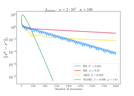
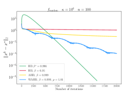
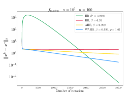
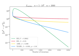
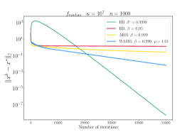
Figure 1: Trajectories of HB, AHB, and WAHB applied to minimize a quadratic function from (26) with different condition numbers $\varkappa$ and dimension $n$.

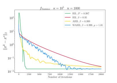
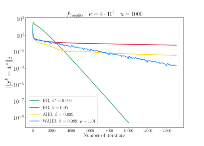
Figure 2: Trajectories of HB, AHB, and WAHB applied to minimize a quadratic functions from (27) and (28) with condition numbers $\varkappa\sim 10^{5}$ and dimension $n=1000$.

These results show that methods with averaging (AHB and WAHB) converge reasonably well during the first iterations of the method even with large $\beta=0.999$, which was larger than the optimal $\beta^{*}$ in all our experiments. Moreover, unlike HB with optimal parameters, AHB and WAHB do not suffer from the peak effect. The absence of peak effect allows us to use HB with averaging for the first iterates and then restart the method. Finally, we emphasize that HB with $\beta=0.95$ converges slower than WAHB with $\beta=0.999$ in all our experiments and slower than AHB with $\beta=0.999$ in almost all experiments (except the first one shown in Figure 1). We also tested HB with $\beta=0.999$ and observed very slow convergence for the method in this case.

To conclude, our experiments on quadratic functions highlight the benefits of using AHB and WAHB with large $\beta$ and standard $\alpha=\nicefrac{{1}}{{L}}$.

4.2 Logistic Regression with $\ell_{2}$-Regularization

Next, we also consider logistic regression with $\ell_{2}$-regularization:

$$\min\limits_{x\in\mathbb{R}^{n}}\left\{f(x)=\frac{1}{m}\sum\limits_{i=1}^{m}\log\left(1+\exp\left(-y_{i}\cdot({\bf A}x)_{i}\right)\right)+\frac{\ell_{2}}{2}\|x\|_{2}^{2}\right\},$$ (29)

where $m$ is the total number of data points/samples, $y_{i}\in\{-1,1\}$ is a label of $i$-th datapoint, and ${\bf A}\in\mathbb{R}^{m\times d}$ is a feature matrix. This function is known to be $\ell_{2}$-strongly convex and $(L+\ell_{2})$-smooth with $L=\nicefrac{{\sigma_{\max}^{2}({\bf A})}}{{4m}}$, where $\sigma_{\max}(A)$ is the maximal singular value of matrix ${\bf A}$. We take the datasets, i.e., pairs of $({\bf A},\{y_{i}\}_{i=1}^{m})$, from LIBSVM library [1], see the summary of the considered datasets in Table 2.

Table 2: Summary of the considered datasets for the logistic regression.

	a9a	phishing	w8a
$m$ (# of data points)	32 561	11 055	49 749
$d$ (# of features)	123	68	300

Algorithm 5 Tail-Averaged Heavy-Ball method (TAHB)

1:starting points $x_{0}$, $x_{1}$ (by default $x_{0}=x_{1}$), number of iterations $N$, stepsize $\alpha>0$, momentum parameter $\beta\in[0,1]$, tail size $s\geq 0$

2:for $k=1,\ldots,N-1$ do

3:     $x_{k+1}=x_{k}-\alpha\nabla f(x_{k})+\beta(x_{k}-x_{k-1})$

4:     $\overline{x}_{k+1}=\begin{cases}\frac{1}{k+2}\sum\limits_{i=0}^{k+1}x_{i},&\text{if }k+1<s,\\ \frac{1}{s}\sum\limits_{i=0}^{s-1}x_{k+1-i},&\text{if }k+1\geq s\end{cases}$ $\triangleright$ It is required to store the last $s$ iterates

5:end for

6:$\overline{x}_{k}$

We run HB, AHB and WAHB with different momentum parameters $\beta$ solve this problem. Moreover, we also tested a modification of AHB called Tail-Averaged Heavy-Ball method (TAHB, see Algorithm 5) with $s\in\{10,50\}$. The weights for WAHB were chosen as $w_{k}=\rho^{k}$ for $\rho\in\{1.1.,1.01\}$. Next, we chose parameter $\beta$ from the set $\{0.9,0.95,0.99,0.999\}$, and tuned stepsize parameter $\alpha\in\{2^{-4},2^{-3},2^{-2},2^{-1},1,2,4,8,16,32,64,128,256\}\cdot\nicefrac{{1}}{{L}}$ for each method separately for given $\beta$ (and for given $\rho$ in case of WAHB, for given $s$ for TAHB). The result are shown in Figures 3-6.

Figures 3-5.

The plots show that for small $\beta$, i.e., $\beta=0.9,0.95$, HB does not have significant oscillations and WAHB and TAHB have comparable performance. However, for larger $\beta$, i.e., $\beta=0.99,0.999$, the behavior of HB is signigicantly non-monotone and oscillations are quite large. In contrast, WAHB and TAHB have much smaller oscillations and converge faster than HB. These facts illustrate the advantages of using proper averaging scheme for HB (either in form of WAHB or TAHB).

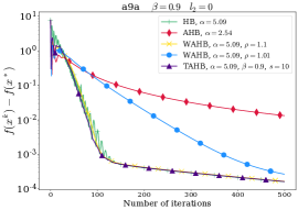
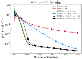
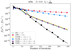
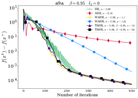
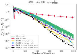
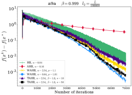
Figure 3: Trajectories of HB, AHB, WAHB, and TAHB with different momentum parameters $\beta$ applied to solve logistic regression problem with $\ell_{2}$-regularization for a9a dataset. Stepsize $\alpha$ was tuned for each method and each choice of $\beta$ (and $\rho$, $s$) separately.

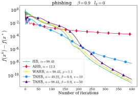
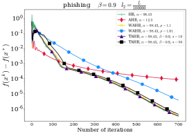
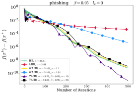
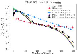
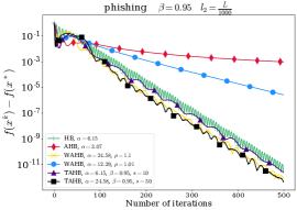
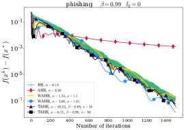
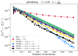
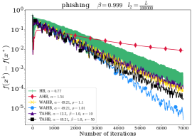
Figure 4: Trajectories of HB, AHB, WAHB, and TAHB with different momentum parameters $\beta$ applied to solve logistic regression problem with $\ell_{2}$-regularization for phishing dataset. Stepsize $\alpha$ was tuned for each method and each choice of $\beta$ (and $\rho$, $s$) separately.

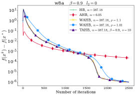
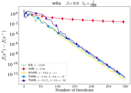
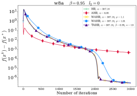
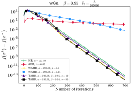
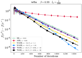
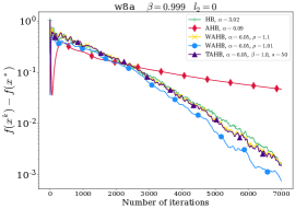
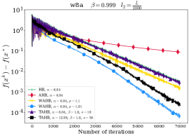
Figure 5: Trajectories of HB, AHB, WAHB, and TAHB with different momentum parameters $\beta$ applied to solve logistic regression problem with $\ell_{2}$-regularization for phishing dataset. Stepsize $\alpha$ was tuned for each method and each choice of $\beta$ (and $\rho$, $s$) separately.

Figure 6.

In these plots, we highlight the effect of averaging for large $\beta$. That is, we compare HB with standard and commonly used choice of $\beta$ ($\beta=0.95$) and TAHB with $\beta=\{0.95,0.99\}$. Moreover, for $\ell_{2}>0$ we also tested HB with optimal parameters from (4). The results for all considered datasets show that TAHB with $\beta=0.95$ has comparable performance with HB and oscillates smaller, while TAHB with $\beta=0.99$ is always slower than TAHB with $\beta=0.95$. Next, when $\ell_{2}=\nicefrac{{L}}{{100000}}$ (ill-conditioned problems), TAHB with $\beta=0.99$ is as fast as HB with optimal parameters but has smaller oscillations. Finally, when $\ell_{2}=\nicefrac{{L}}{{1000}}$ (well-conditioned problems), HB with optimal parameters has negligible oscillations and shows the best performance. Such behavior is natural since for the well-conditioned problems HB does not suffer significantly from the non-monotone behavior and peak-effect.

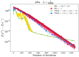
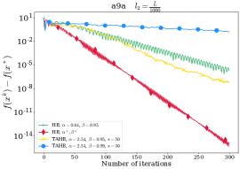
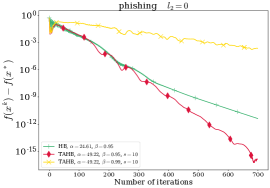
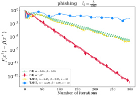
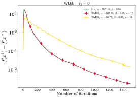
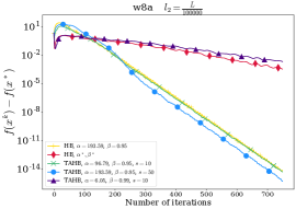
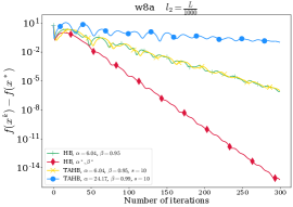
Figure 6: Trajectories of HB with $\beta=0.95$ (standard choice of $\beta$) and TAHB with $\beta=0.95$ and $\beta=0.99$ (large $\beta$) applied to solve logistic regression problem with $\ell_{2}$-regularization for dataset from Table 2. Stepsize parameter $\alpha$ was tuned for each method separately. For $\ell_{2}>0$ we also show the trajectories of HB with optimal parameters $\alpha=\alpha^{*}$ and $\beta=\beta^{*}$ from (4).

5 Conclusion

This paper shows the advantages of using averaging for Heavy-Ball method both in theory and practice. That is, our theory and experiments imply that averaging helps to reduce the oscillations of HB. Although the derived theoretical convergence guarantees for HB with averaging are not better than existing ones for HB, in our experiments, we observe that HB with properly adjusted averaging scheme can converge faster than HB without averaging. In particular, we observe this phenomenon when momentum parameter $\beta$ for averaged versions of HB is chosen to be large enough, e.g., larger than the standard choice of $\beta=0.95$ and sometimes larger than the optimal choice of $\beta$ from (4).

Appendix A Basic Inequalities

For all $a,b\in\mathbb{R}^{n}$ and $\lambda>0,q\in(0,1]$

$$|\langle a,b\rangle|\leq\frac{\|a\|_{2}^{2}}{2\lambda}+\frac{\lambda\|b\|_{2}^{2}}{2},$$ (30)

$$\|a+b\|_{2}^{2}\leq 2\|a\|_{2}^{2}+2\|b\|_{2}^{2},$$ (31)

$$\|a+b\|^{2}\leq(1+\lambda)\|a\|^{2}+\left(1+\frac{1}{\lambda}\right)\|b\|^{2},$$ (32)

$$\langle a,b\rangle=\frac{1}{2}\left(\|a+b\|_{2}^{2}-\|a\|_{2}^{2}-\|b\|_{2}^{2}\right),$$ (33)

$$\left(1-\frac{q}{2}\right)^{-1}\leq 1+q,$$ (34)

$$\left(1+\frac{q}{2}\right)(1-q)\leq 1-\frac{q}{2}.$$ (35)

Appendix B Auxiliary Results

Lemma B.1.

Lemma 1 from [10] Let $\rho_{1}$ and $\rho_{2}$ be the eigenvalues of the matrix ${\bf M}=\begin{bmatrix}a&b\\ 1&0\end{bmatrix}$ and let $k$ be a positive integer. If $\rho_{1}\neq\rho_{2}$, then we have

$${\bf M}^{k}=\frac{1}{\rho_{2}-\rho_{1}}\begin{bmatrix}\rho_{2}^{k+1}-\rho_{1}^{k+1}&\rho_{1}\rho_{2}(\rho_{1}^{k}-\rho_{2}^{k})\\ \rho_{2}^{k}-\rho_{1}^{k}&\rho_{1}\rho_{2}(\rho_{1}^{k-1}-\rho_{2}^{k-1})\end{bmatrix}.$$

Moreover, if $\rho_{1}=\rho_{2}=\rho$, the matrix ${\bf M}^{k}$ satisfies

$${\bf M}^{k}=\begin{bmatrix}(k+1)\rho^{k}&-k\rho^{k+1}\\ k\rho^{k-1}&(1-k)\rho^{k}\end{bmatrix}.$$

Appendix C Missing Proofs from Section 2

In this section, for $x$, we use the upper index for an iteration counter, and the lower index denotes the component of the vector.

C.1 Proof of Theorem 2.2

Rewriting the update rule of HB for $f(x)=\frac{1}{2}x^{\top}{\bf A}x$ with ${\bf A}=\mathrm{diag}\left(\mu,\ \lambda_{2},\ \ldots,\ \lambda_{n-1},L\right)$ with $\alpha=\frac{1}{L}$ we get

$$x_{1}^{k+1} = \left(1-\frac{\mu}{L}+\beta\right)x_{1}^{k}-\beta x_{1}^{k-1},$$

$$x_{2}^{k+1} = \left(1-\frac{\lambda_{2}}{L}+\beta\right)x_{2}^{k}-\beta x_{2}^{k-1},$$

$$\vdots$$

$$x_{n-1}^{k+1} = \left(1-\frac{\lambda_{n-1}}{L}+\beta\right)x_{n-1}^{k}-\beta x_{n-1}^{k-1},$$

$$x_{n}^{k+1} = \beta x_{n}^{k}-\beta x_{n}^{k-1}.$$

To solve these recurrences we consider the corresponding characteristic equations:

$$\rho^{2} = \left(1-\frac{\mu}{L}+\beta\right)\rho-\beta,$$

$$\rho^{2} = \left(1-\frac{\lambda_{2}}{L}+\beta\right)\rho-\beta,$$

$$\vdots$$

$$\rho^{2} = \left(1-\frac{\lambda_{n-1}}{L}+\beta\right)\rho-\beta,$$

$$\rho^{2} = \beta\rho-\beta.$$

Since $\beta\leq(1-2\sqrt{\nicefrac{{\mu}}{{L}}})^{2}<(1-\sqrt{\nicefrac{{\mu}}{{L}}})^{2}$ the roots of the first equation are

$$\rho_{1}(\mu) = \frac{1+\beta-\nicefrac{{\mu}}{{L}}+\sqrt{\left(1+\beta-\nicefrac{{\mu}}{{L}}\right)^{2}-4\beta}}{2},$$

$$\rho_{2}(\mu) = \frac{1+\beta-\nicefrac{{\mu}}{{L}}-\sqrt{\left(1+\beta-\nicefrac{{\mu}}{{L}}\right)^{2}-4\beta}}{2}.$$

Moreover, we have $\sqrt{\left(1+\beta-\nicefrac{{\mu}}{{L}}\right)^{2}-4\beta}\leq 1-\beta+\nicefrac{{\mu}}{{L}}$, and, as a consequence, $0<\rho_{2}(\mu)<\rho_{1}(\mu)<1$. Next, the first components of iterates produced by HB satisfy

$$x_{1}^{k}=C_{1}\rho_{1}^{k}(\mu)+C_{2}\rho_{2}^{k}(\mu)$$

with some constants $C_{1},C_{2}\in\mathbb{R}$. This equation and the choice of the starting points $x^{0}=x^{1}=(1,1,\ldots,1)^{\top}$ imply

$$\begin{cases}C_{1}+C_{2}&=1,\\ C_{1}\rho_{1}(\mu)+C_{2}\rho_{2}(\mu)&=1,\end{cases}$$

whence

$$C_{1}=\frac{1-\rho_{2}(\mu)}{\rho_{1}(\mu)-\rho_{2}(\mu)},\quad C_{2}=1-C_{1}=\frac{\rho_{1}(\mu)-1}{\rho_{1}(\mu)-\rho_{2}(\mu)}.$$

Using the formula for $C_{1}$ and $\beta\in[(1-3\sqrt{\nicefrac{{\mu}}{{L}}})^{2},(1-2\sqrt{\nicefrac{{\mu}}{{L}}})^{2}]$ we derive that $C_{1}>0$ and

$$C_{1} = \left(1-\frac{1+\beta-\nicefrac{{\mu}}{{L}}-\sqrt{\left(1+\beta-\nicefrac{{\mu}}{{L}}\right)^{2}-4\beta}}{2}\right)\frac{1}{\sqrt{\left(1+\beta-\nicefrac{{\mu}}{{L}}\right)^{2}-4\beta}}$$

$$= \frac{1-\beta+\nicefrac{{\mu}}{{L}}+\sqrt{\left(1+\beta-\nicefrac{{\mu}}{{L}}\right)^{2}-4\beta}}{2\sqrt{\left(1+\beta-\nicefrac{{\mu}}{{L}}\right)^{2}-4\beta}}$$

$$= \frac{1}{2}+\frac{1-\beta+\nicefrac{{\mu}}{{L}}}{2\sqrt{\left(1+\beta-\nicefrac{{\mu}}{{L}}\right)^{2}-4\beta}}$$

$$\leq \frac{1}{2}+\frac{1-(1-3\sqrt{\nicefrac{{\mu}}{{L}}})^{2}+\nicefrac{{\mu}}{{L}}}{2\sqrt{\left(1+(1-2\sqrt{\nicefrac{{\mu}}{{L}}})^{2}-\nicefrac{{\mu}}{{L}}\right)^{2}-4(1-2\sqrt{\nicefrac{{\mu}}{{L}}})^{2}}}$$

$$= \frac{1}{2}+\frac{3\sqrt{\nicefrac{{\mu}}{{L}}}-4\nicefrac{{\mu}}{{L}}}{\sqrt{\left(2-4\sqrt{\nicefrac{{\mu}}{{L}}}+3\nicefrac{{\mu}}{{L}}\right)^{2}-(2-4\sqrt{\nicefrac{{\mu}}{{L}}})^{2}}}$$

$$= \frac{1}{2}+\frac{3\sqrt{\nicefrac{{\mu}}{{L}}}-4\nicefrac{{\mu}}{{L}}}{\sqrt{3\nicefrac{{\mu}}{{L}}\left(4-8\sqrt{\nicefrac{{\mu}}{{L}}}+3\nicefrac{{\mu}}{{L}}\right)}}.$$

Since $L\geq 100\mu$ we can further upper bound the right-hand side of the previous inequality and get

$$C_{1} \leq \frac{1}{2}+\frac{3\sqrt{\nicefrac{{\mu}}{{L}}}}{\sqrt{3\nicefrac{{\mu}}{{L}}\left(4-8\sqrt{\nicefrac{{\mu}}{{L}}}\right)}}\leq\frac{1}{2}+\frac{\sqrt{3}}{\sqrt{4-\nicefrac{{4}}{{5}}}}=\frac{1}{2}+\frac{1}{2}\sqrt{\frac{15}{4}}\leq\frac{3}{2}.$$

Taking into account that $C_{1}>0$ and $C_{2}=1-C_{1}$ we derive that $|C_{2}|=\max\{1-C_{1},C_{1}-1\}\leq\nicefrac{{1}}{{2}}$. Putting all together, we obtain

$$|x_{1}^{k}|=|C_{1}\rho_{1}^{k}(\mu)+C_{2}\rho_{2}^{k}(\mu)|\leq|C_{1}|+|C_{2}|\leq 2\quad\forall k\geq 0$$

In the remaining part of the proof, we handle the characteristic equations

$$\rho^{2} = \left(1-\frac{\lambda_{2}}{L}+\beta\right)\rho-\beta,$$

$$\vdots$$

$$\rho^{2} = \left(1-\frac{\lambda_{n-1}}{L}+\beta\right)\rho-\beta,$$

$$\rho^{2} = \beta\rho-\beta.$$

Without loss of generality, we consider the equation

$$\rho^{2}=\left(1-\frac{\lambda}{L}+\beta\right)\rho-\beta$$ (36)

with $\lambda\in[\lambda_{2},L]$. This equation serves as a characteristic equation for the sequence $\{y_{k}\}_{k\geq 0}\subseteq\mathbb{R}$ satisfying

$$y_{k+1}=\left(1-\frac{\lambda}{L}+\beta\right)y_{k}-\beta y_{k-1}.$$

Since $\lambda\geq\lambda_{2}\geq 10\mu$ and $\beta\geq(1-3\sqrt{\nicefrac{{\mu}}{{L}}})^{2}$ we conclude that $\beta\geq(1-\sqrt{\nicefrac{{\lambda}}{{L}}})^{2}$ and the characteristic equation has the complex roots with non-zero imaginary parts:

$$\rho_{1}(\lambda) = \frac{1+\beta-\nicefrac{{\lambda}}{{L}}+i\sqrt{4\beta-\left(1+\beta-\nicefrac{{\mu}}{{L}}\right)^{2}}}{2},$$

$$\rho_{2}(\lambda) = \frac{1+\beta-\nicefrac{{\mu}}{{L}}-i\sqrt{4\beta-\left(1+\beta-\nicefrac{{\mu}}{{L}}\right)^{2}}}{2}.$$

This implies that $|\rho_{1}(\lambda)|=|\rho_{1}(\lambda)|=\sqrt{\beta}<1$ and

$$y_{k}=C_{1}\rho_{1}^{k}(\lambda)+C_{2}\rho_{2}^{k}(\lambda)$$

for some complex numbers $C_{1},C_{2}$. Let $y_{0}=y_{1}=1$. Then,

$$\begin{cases}C_{1}+C_{2}&=1,\\ C_{1}\rho_{1}(\lambda)+C_{2}\rho_{2}(\lambda)&=1,\end{cases}$$

whence

$$C_{1}=\frac{1-\rho_{2}(\lambda)}{\rho_{1}(\lambda)-\rho_{2}(\lambda)},\quad C_{2}=1-C_{1}=\frac{\rho_{1}(\lambda)-1}{\rho_{1}(\lambda)-\rho_{2}(\lambda)}.$$

Using the formula for $C_{1}$ and $\beta\in[(1-3\sqrt{\nicefrac{{\mu}}{{L}}})^{2},(1-2\sqrt{\nicefrac{{\mu}}{{L}}})^{2}]$ we derive that

$$C_{1} = \left(1-\frac{1+\beta-\nicefrac{{\lambda}}{{L}}-i\sqrt{4\beta-\left(1+\beta-\nicefrac{{\lambda}}{{L}}\right)^{2}}}{2}\right)\frac{1}{i\sqrt{4\beta-\left(1+\beta-\nicefrac{{\lambda}}{{L}}\right)^{2}}}$$

$$= \frac{1-\beta+\nicefrac{{\lambda}}{{L}}+i\sqrt{4\beta-\left(1+\beta-\nicefrac{{\lambda}}{{L}}\right)^{2}}}{2i\sqrt{4\beta-\left(1+\beta-\nicefrac{{\lambda}}{{L}}\right)^{2}}}$$

$$= \frac{1}{2}-i\frac{1-\beta+\nicefrac{{\lambda}}{{L}}}{2\sqrt{4\beta-\left(1+\beta-\nicefrac{{\lambda}}{{L}}\right)^{2}}}.$$

Then, for the absolute value of $C_{1}$ we have

$$|C_{1}| = \frac{1}{2}\sqrt{1+\frac{(1+\nicefrac{{\lambda}}{{L}}-\beta)^{2}}{4\beta-(1-\nicefrac{{\lambda}}{{L}}+\beta)^{2}}}$$

$$\leq \frac{1}{2}\sqrt{1+\frac{\left(1+\nicefrac{{\lambda}}{{L}}-\left(1-3\sqrt{\nicefrac{{\mu}}{{L}}}\right)^{2}\right)^{2}}{4\left(1-2\sqrt{\nicefrac{{\mu}}{{L}}}\right)^{2}-\left(1-\nicefrac{{\lambda}}{{L}}+\left(1-2\sqrt{\nicefrac{{\mu}}{{L}}}\right)^{2}\right)^{2}}}$$

$$= \frac{1}{2}\sqrt{1+\frac{\left(\nicefrac{{\lambda}}{{L}}-9\nicefrac{{\mu}}{{L}}+6\sqrt{\nicefrac{{\mu}}{{L}}}\right)^{2}}{\left(2-4\sqrt{\nicefrac{{\mu}}{{L}}}\right)^{2}-\left(2-\nicefrac{{\lambda}}{{L}}-4\sqrt{\nicefrac{{\mu}}{{L}}}+4\nicefrac{{\mu}}{{L}}\right)^{2}}}$$

$$= \frac{1}{2}\sqrt{1+\frac{\left(\nicefrac{{\lambda}}{{L}}-9\nicefrac{{\mu}}{{L}}+6\sqrt{\nicefrac{{\mu}}{{L}}}\right)^{2}}{\left(4-\nicefrac{{\lambda}}{{L}}-8\sqrt{\nicefrac{{\mu}}{{L}}}+4\nicefrac{{\mu}}{{L}}\right)\left(\nicefrac{{\lambda}}{{L}}-4\nicefrac{{\mu}}{{L}}\right)}}$$

$$\leq \frac{1}{2}\sqrt{1+\frac{\left(\nicefrac{{\lambda}}{{L}}+6\sqrt{\nicefrac{{\mu}}{{L}}}\right)^{2}}{\left(3-\nicefrac{{4}}{{5}}\right)\left(\nicefrac{{\lambda}}{{L}}-\nicefrac{{2\lambda}}{{5L}}\right)}}=\frac{1}{2}\sqrt{1+\frac{25}{33}\frac{\nicefrac{{\lambda^{2}}}{{L^{2}}}+12\nicefrac{{(\lambda\sqrt{\mu})}}{{(L\sqrt{L})}}+36\nicefrac{{\mu}}{{L}}}{\nicefrac{{\lambda}}{{L}}}}$$

$$= \frac{1}{2}\sqrt{1+\frac{25}{33}\left(\frac{\lambda}{L}+12\sqrt{\frac{\mu}{L}}+36\frac{\mu}{\lambda}\right)}\leq\frac{1}{2}\sqrt{1+\frac{25}{33}\left(1+\frac{6}{5}+\frac{8}{25}\right)}\leq 1.$$

Since

$$C_{2}=1-C_{1}=\frac{1}{2}+i\frac{1-\beta+\nicefrac{{\lambda}}{{L}}}{2\sqrt{4\beta-\left(1+\beta-\nicefrac{{\lambda}}{{L}}\right)^{2}}}$$

we also have $|C_{2}|=|C_{1}|\leq 1$, and, as a consequence,

$$|y_{k}|=|C_{1}\rho_{1}^{k}(\lambda)+C_{2}\rho_{2}^{k}(\lambda)|\leq|C_{1}|+|C_{2}|\leq 2\quad\forall k\geq 0.$$

This result implies that $|x_{i}^{k}|\leq 2$ for all $k\geq 0$ and $i=2,\ldots,n$.

Finally, since $\overline{x}^{k}=\frac{1}{k+1}\sum_{t=0}^{k}x^{t}$ we conclude that

$$|\overline{x}_{i}^{k}|\leq\frac{1}{k+1}\sum\limits_{t=0}^{k}|x_{i}^{t}|\leq 2\quad\forall k\geq 0,\;i=1,\ldots,n$$

that is equivalent to (6).

C.2 Proof of Theorem 2.3

To estimate $\text{dev}_{{\sf HB}}(\alpha,\beta)$ we consider the spectral decomposition of matrix ${\bf A}={\bf U}{\bf\Lambda}{\bf U}^{\top}\succ 0$, where ${\bf\Lambda}=\mathrm{diag}(\lambda_{1},\ldots,\lambda_{n})$ is a diagonal matrix of the eigenvalues of ${\bf A}$, $\lambda_{1}\leq\ldots\leq\lambda_{n}$, and $U$ is a unitary matrix of the eigenvectors of ${\bf A}$. Next, without loss of the generality we assume that $x^{*}=0$. Applying the unitary transformation ${\bf U}^{\top}$ to $x^{k}$ we obtain $\hat{x}^{k}={\bf U}^{\top}x^{k}$ and

$$\hat{z}^{k}:=\begin{bmatrix}\hat{x}^{k+1}\\ \hat{x}^{k}\end{bmatrix}=\hat{\bf T}\begin{bmatrix}\hat{x}^{k}\\ \hat{x}^{k-1}\end{bmatrix}=\ldots=\hat{\bf T}^{k}\begin{bmatrix}\hat{x}^{1}\\ \hat{x}^{0}\end{bmatrix},$$

where

$$\hat{\bf T}=\left[\begin{array}[]{@{}c|c@{}}\begin{matrix}(1+\beta){\bf I}-\alpha{\bf\Lambda}\end{matrix}&-\beta{\bf I}\\ \hline\cr{\bf I}&{\bf 0}\end{array}\right]=\left[\begin{array}[]{@{}c|c@{}}{\bf U}^{\top}&{\bf 0}\\ \hline\cr{\bf 0}&{\bf U}^{\top}\end{array}\right]{\bf T}.$$

In particular, these formulas imply

$$\begin{bmatrix}\hat{x}_{j}^{k+1}\\ \hat{x}_{j}^{k}\end{bmatrix}=\hat{\bf T}_{j}\begin{bmatrix}\hat{x}_{j}^{k}\\ \hat{x}_{j}^{k-1}\end{bmatrix}=\ldots=\hat{\bf T}_{j}^{k}\begin{bmatrix}\hat{x}_{j}^{1}\\ \hat{x}_{j}^{0}\end{bmatrix},$$

where

$$\hat{\bf T}_{j}=\begin{bmatrix}1+\beta-\alpha\lambda_{j}&-\beta\\ 1&0\end{bmatrix}$$

for all $j=1,\ldots,n$. Moreover, $\|{\bf C}{\bf T}^{k}\|_{2}=\max\limits_{j=1,\ldots,n}\|{\bf C}_{j}\hat{\bf T}_{j}^{k}\|_{2}$, where ${\bf C}_{j}=\begin{bmatrix}0&1\end{bmatrix}$.

It is easy to see that the eigenvalues of $\hat{\bf T}_{j}$ are

$$\rho_{j,1}=\frac{1+\beta-\nicefrac{{\lambda_{j}}}{{\lambda_{n}}}+\sqrt{(1+\beta-\nicefrac{{\lambda_{j}}}{{\lambda_{n}}})^{2}-4\beta}}{2},\quad\rho_{j,2}=\frac{1+\beta-\nicefrac{{\lambda_{j}}}{{\lambda_{n}}}-\sqrt{(1+\beta-\nicefrac{{\lambda_{j}}}{{\lambda_{n}}})^{2}-4\beta}}{2}$$

for all $\lambda_{j}$ such that $(1+\beta-\nicefrac{{\lambda_{j}}}{{\lambda_{n}}})^{2}-4\beta>0$ and

$$\rho_{j,1}=\frac{1+\beta-\nicefrac{{\lambda_{j}}}{{\lambda_{n}}}+i\sqrt{4\beta-(1+\beta-\nicefrac{{\lambda_{j}}}{{\lambda_{n}}})^{2}}}{2},\quad\rho_{j,2}=\frac{1+\beta-\nicefrac{{\lambda_{j}}}{{\lambda_{n}}}-i\sqrt{4\beta-(1+\beta-\nicefrac{{\lambda_{j}}}{{\lambda_{n}}})^{2}}}{2}$$

for all $\lambda_{j}$ such that $(1+\beta-\nicefrac{{\lambda_{j}}}{{\lambda_{n}}})^{2}-4\beta<0$. Taking into account the assumptions of the theorem, we derive

$$\rho_{1,1}=\frac{1+\beta-\nicefrac{{\lambda_{1}}}{{\lambda_{n}}}+\sqrt{(1+\beta-\nicefrac{{\lambda_{1}}}{{\lambda_{n}}})^{2}-4\beta}}{2},\quad\rho_{1,2}=\frac{1+\beta-\nicefrac{{\lambda_{1}}}{{\lambda_{n}}}-\sqrt{(1+\beta-\nicefrac{{\lambda_{1}}}{{\lambda_{n}}})^{2}-4\beta}}{2}$$

and

$$\rho_{j,1}=\frac{1+\beta-\nicefrac{{\lambda_{j}}}{{\lambda_{n}}}+i\sqrt{4\beta-(1+\beta-\nicefrac{{\lambda_{j}}}{{\lambda_{n}}})^{2}}}{2},\quad\rho_{j,2}=\frac{1+\beta-\nicefrac{{\lambda_{j}}}{{\lambda_{n}}}-i\sqrt{4\beta-(1+\beta-\nicefrac{{\lambda_{j}}}{{\lambda_{n}}})^{2}}}{2}$$

for all $j=2,\ldots,n$. Moreover, $|\rho_{j,1}|=|\rho_{j,2}|=\sqrt{\beta}$.

Next, using Lemma B.1 we get

$$\|{\bf C}_{j}\hat{\bf T}_{j}^{k}\|_{2} = \left\|\frac{1}{\rho_{j,2}-\rho_{j,1}}\begin{bmatrix}0&1\end{bmatrix}\begin{bmatrix}\rho_{j,2}^{k+1}-\rho_{j,1}^{k+1}&\rho_{j,1}\rho_{j,2}(\rho_{j,1}^{k}-\rho_{j,2}^{k})\\ \rho_{j,2}^{k}-\rho_{j,1}^{k}&\rho_{j,1}\rho_{j,2}(\rho_{j,1}^{k-1}-\rho_{j,2}^{k-1})\end{bmatrix}\right\|_{2}$$ (37)

$$= \sqrt{\left|\frac{\rho_{j,2}^{k}-\rho_{j,1}^{k}}{\rho_{j,2}-\rho_{j,1}}\right|^{2}+\left|\frac{\rho_{j,1}\rho_{j,2}\left(\rho_{j,2}^{k-1}-\rho_{j,1}^{k-1}\right)}{\rho_{j,2}-\rho_{j,1}}\right|^{2}}$$

$$\leq \sqrt{\left(\sum\limits_{t=0}^{k-1}|\rho_{j,1}|^{k-1-t}|\rho_{j,2}|^{t}\right)^{2}+\left(|\rho_{j,1}||\rho_{j,2}|\sum\limits_{t=0}^{k-2}|\rho_{j,1}|^{k-2-t}|\rho_{j,2}|^{t}\right)^{2}}.$$

Consider the expression above for $j=1$. To bound the sums appearing in the right-hand side of the previous inequality we derive:

$$\frac{|\rho_{1,2}|}{|\rho_{1,1}|} = \frac{1+\beta-\nicefrac{{\lambda_{1}}}{{\lambda_{n}}}-\sqrt{(1+\beta-\nicefrac{{\lambda_{1}}}{{\lambda_{n}}})^{2}-4\beta}}{1+\beta-\nicefrac{{\lambda_{1}}}{{\lambda_{n}}}+\sqrt{(1+\beta-\nicefrac{{\lambda_{1}}}{{\lambda_{n}}})^{2}-4\beta}}$$

$$= 1-\frac{2\sqrt{(1+\beta-\nicefrac{{\lambda_{1}}}{{\lambda_{n}}})^{2}-4\beta}}{1+\beta-\nicefrac{{\lambda_{1}}}{{\lambda_{n}}}+\sqrt{(1+\beta-\nicefrac{{\lambda_{1}}}{{\lambda_{n}}})^{2}-4\beta}}$$

$$\leq 1-\frac{2\sqrt{\left(1+\left(1-F\sqrt{\nicefrac{{\lambda_{1}}}{{\lambda_{n}}}}\right)^{2}-\nicefrac{{\lambda_{1}}}{{\lambda_{n}}}\right)^{2}-4\left(1-F\sqrt{\nicefrac{{\lambda_{1}}}{{\lambda_{n}}}}\right)^{2}}}{2-\nicefrac{{\lambda_{1}}}{{\lambda_{n}}}+\sqrt{(1-\nicefrac{{\lambda_{1}}}{{\lambda_{n}}})^{2}}}$$

$$= 1-\frac{2\sqrt{\left(2-2F\sqrt{\nicefrac{{\lambda_{1}}}{{\lambda_{n}}}}+(F^{2}-1)\nicefrac{{\lambda_{1}}}{{\lambda_{n}}}\right)^{2}-4\left(1-F\sqrt{\nicefrac{{\lambda_{1}}}{{\lambda_{n}}}}\right)^{2}}}{3-2\nicefrac{{\lambda_{1}}}{{\lambda_{n}}}}$$

$$\leq 1-\frac{2\sqrt{(F^{2}-1)\nicefrac{{\lambda_{1}}}{{\lambda_{n}}}\left(4-4F\sqrt{\nicefrac{{\lambda_{1}}}{{\lambda_{n}}}}+(F^{2}-1)\nicefrac{{\lambda_{1}}}{{\lambda_{n}}}\right)}}{3}$$

$$= 1-\frac{2\sqrt{(F^{2}-1)\left(\left(2-F\sqrt{\nicefrac{{\lambda_{1}}}{{\lambda_{n}}}}\right)^{2}-\nicefrac{{\lambda_{1}}}{{\lambda_{n}}}\right)}}{3\sqrt{\varkappa}}\leq 1-\frac{\sqrt{F^{2}-1}}{\sqrt{3\varkappa}},$$

where the first inequality follows from the fact the function $g(\beta)=(1+\beta-\nicefrac{{\lambda_{1}}}{{\lambda_{n}}})^{2}-4\beta$ is decreasing for $\beta\leq(1-\sqrt{\nicefrac{{\lambda_{1}}}{{\lambda_{n}}}})^{2}$, and in the last inequality we apply $1-F\sqrt{\nicefrac{{\lambda_{1}}}{{\lambda_{n}}}}\geq 0$, $\nicefrac{{\lambda_{1}}}{{\lambda_{n}}}\leq\nicefrac{{1}}{{10000}}<\nicefrac{{1}}{{4}}$, and $\varkappa=\nicefrac{{\lambda_{n}}}{{\lambda_{1}}}$. Therefore,

$$\sum\limits_{t=0}^{k-1}|\rho_{1,1}|^{k-1-t}|\rho_{1,2}|^{t} = |\rho_{1,1}|^{k-1}\sum\limits_{t=0}^{k-1}\left(\frac{|\rho_{1,2}|}{|\rho_{1,1}|}\right)^{t}\leq\sum\limits_{t=0}^{\infty}\left(1-\frac{\sqrt{F^{2}-1}}{\sqrt{3\varkappa}}\right)^{t}=\frac{\sqrt{3\varkappa}}{\sqrt{F^{2}-1}}$$

and, similarly,

$$|\rho_{j,1}||\rho_{j,2}|\sum\limits_{t=0}^{k-2}|\rho_{j,1}|^{k-2-t}|\rho_{j,2}|^{t} \leq \sum\limits_{t=0}^{k-2}\left(\frac{|\rho_{1,2}|}{|\rho_{1,1}|}\right)^{t}\leq\sum\limits_{t=0}^{\infty}\left(1-\frac{\sqrt{F^{2}-1}}{\sqrt{3\varkappa}}\right)^{t}=\frac{\sqrt{3\varkappa}}{\sqrt{F^{2}-1}}.$$

Plugging these upper bounds in (37) we derive

$$\|{\bf C}_{j}\hat{\bf T}_{j}^{k}\|_{2}\leq\frac{\sqrt{6\varkappa}}{\sqrt{F^{2}-1}}.$$ (38)

Next, we consider the right-hand side of (37) for $j=2,\ldots,n$. In this case, $|\rho_{j,1}|=|\rho_{j,2}|=\sqrt{\beta}\leq 1-\nicefrac{{F}}{{\sqrt{\varkappa}}}$. Therefore,

$$\sum\limits_{t=0}^{k-1}|\rho_{j,1}|^{k-1-t}|\rho_{j,2}|^{t} = k\left(\sqrt{\beta}\right)^{k-1}\leq k\left(1-\frac{F}{\sqrt{\varkappa}}\right)^{k-1}\leq(k-1)\exp\left(-(k-1)\frac{F}{\sqrt{\varkappa}}\right)+1$$

and, similarly,

$$|\rho_{j,1}||\rho_{j,2}|\sum\limits_{t=0}^{k-2}|\rho_{j,1}|^{k-2-t}|\rho_{j,2}|^{t} = (k-1)\left(\sqrt{\beta}\right)^{k}\leq(k-1)\exp\left(-(k-1)\frac{F}{\sqrt{\varkappa}}\right).$$

Since the maximal value of the function $g(x)=xa^{x}$ for $x\geq 0$ equals $-\nicefrac{{1}}{{(e\ln(a))}}$, we have

$$(k-1)\exp\left(-(k-1)\frac{F}{\sqrt{\varkappa}}\right)\leq-\frac{1}{e\ln\left(\exp\left(-\frac{F}{\sqrt{\varkappa}}\right)\right)}=\frac{\sqrt{\varkappa}}{eF}.$$

Putting all together we obtain for all $j=2,\ldots,n$

$$\|{\bf C}_{j}\hat{\bf T}_{j}^{k}\|_{2}\overset{\eqref{eq:max_dev_HB_technical_1}}{\leq}\sqrt{\left(\frac{\sqrt{\varkappa}}{eF}+1\right)^{2}+\frac{\varkappa}{e^{2}F^{2}}}\leq\frac{\sqrt{5\varkappa}}{eF},$$ (39)

where we use $F\leq\sqrt{\varkappa}$.

Finally, with (38) and (39) in hand we derive

$$\text{dev}_{{\sf AHB}}(\alpha,\beta)\leq\text{dev}_{{\sf HB}}(\alpha,\beta)=\|{\bf C}{\bf T}^{k}\|_{2}=\max\limits_{j=1,\ldots,n}\|{\bf C}_{j}\hat{\bf T}_{j}^{k}\|_{2}\leq\frac{\sqrt{6\varkappa}}{\sqrt{F^{2}-1}}.$$

Theorem 1 from [3] implies that

$$\text{dev}_{{\sf HB}}(\alpha^{*},\beta^{*})\geq\frac{\sqrt{\varkappa}}{2e},$$

where $\alpha^{*}$ and $\beta^{*}$ are given in (4). Therefore,

$$\text{dev}_{{\sf AHB}}(\alpha,\beta)\leq\text{dev}_{{\sf HB}}(\alpha,\beta)\leq\frac{2e\sqrt{6}}{\sqrt{F^{2}-1}}\text{dev}_{{\sf HB}}(\alpha^{*},\beta^{*}).$$

Appendix D Missing Proofs from Section 3

D.1 Proof of Lemma 3.2

Using recursion (13) for the virtual iterates defined in (12), we derive

$$\|\widetilde{x}_{k+1}-x_{*}\|^{2} = \|\widetilde{x}_{k}-x_{*}\|^{2}-\frac{2\alpha}{1-\beta}\langle\widetilde{x}_{k}-x_{*},\nabla f(x_{k})\rangle+\frac{\alpha^{2}}{(1-\beta)^{2}}\|\nabla f(x_{k})\|^{2}$$ (40)

$$= \|\widetilde{x}_{k}-x_{*}\|^{2}-\frac{2\alpha}{1-\beta}\langle x_{k}-x_{*},\nabla f(x_{k})\rangle+\frac{2\alpha}{1-\beta}\langle x_{k}-\widetilde{x}_{k},\nabla f(x_{k})\rangle$$

$$\quad+\frac{\alpha^{2}}{(1-\beta)^{2}}\|\nabla f(x_{k})\|^{2}.$$

From $\mu$-strong convexity and $L$-smoothness of $f$ we have (e.g., see [13])

$$\langle x_{k}-x_{*},\nabla f(x_{k})\rangle \geq f(x_{k})-f(x_{*})+\frac{\mu}{2}\|x_{k}-x_{*}\|^{2}$$

$$\|\nabla f(x_{k})\|^{2} \leq 2L\left(f(x_{k})-f(x_{*})\right).$$ (41)

Together with (40) these relations give

$$\|\widetilde{x}_{k+1}-x_{*}\|^{2} \leq \|\widetilde{x}_{k}-x_{*}\|^{2}-\frac{\alpha\mu}{1-\beta}\|x_{k}-x_{*}\|^{2}-\frac{2\alpha}{1-\beta}\left(1-\frac{\alpha L}{1-\beta}\right)\left(f(x_{k})-f(x_{*})\right)$$

$$\quad+\frac{2\alpha}{1-\beta}\langle x_{k}-\widetilde{x}_{k},\nabla f(x_{k})\rangle.$$

Next, we estimate the second and the fourth terms in the inequality above. Since $\|a+b\|^{2}\geq\frac{1}{2}\|a\|^{2}-\|b\|^{2}$ for all $a,b\in\mathbb{R}^{n}$ (see also (31)), we can estimate the second term as

$$-\frac{\alpha\mu}{1-\beta}\|x_{k}-x_{*}\|^{2}\leq-\frac{\alpha\mu}{2(1-\beta)}\|\widetilde{x}_{k}-x_{*}\|^{2}+\frac{\alpha\mu}{1-\beta}\|x_{k}-\widetilde{x}_{k}\|^{2}.$$

Using Fenchel-Young inequality (30), we derive

$$\frac{2\alpha}{1-\beta}\langle x_{k}-\widetilde{x}_{k},\nabla f(x_{k})\rangle \leq \frac{2\alpha L}{1-\beta}\|x_{k}-\widetilde{x}_{k}\|^{2}+\frac{2\alpha}{4L(1-\beta)}\|\nabla f(x_{k})\|^{2}$$

$$\overset{\eqref{eq:L_smoothness_cor}}{\leq} \frac{2\alpha L}{1-\beta}\|x_{k}-\widetilde{x}_{k}\|^{2}+\frac{\alpha}{1-\beta}\left(f(x_{k})-f(x_{*})\right).$$

Putting all togetherm, we obtain

$$\|\widetilde{x}_{k+1}-x_{*}\|^{2} \leq \left(1-\frac{\alpha\mu}{2(1-\beta)}\right)\|\widetilde{x}_{k}-x_{*}\|^{2}-\frac{2\alpha}{1-\beta}\left(\frac{1}{2}-\frac{\alpha L}{1-\beta}\right)\left(f(x_{k})-f(x_{*})\right)$$

$$\quad+\frac{\alpha}{1-\beta}\left(2L+\mu\right)\|x_{k}-\widetilde{x}_{k}\|^{2}$$

$$\overset{\eqref{eq:virtual_iterates_HB},\eqref{eq:params_WAHB_1}}{\leq} \left(1-\frac{\alpha\mu}{2(1-\beta)}\right)\|\widetilde{x}_{k}-x_{*}\|^{2}-\frac{\alpha}{1-\beta}\left(f(x_{k})-f(x_{*})\right)+\frac{3L\alpha\beta^{2}}{(1-\beta)^{3}}\|m_{k-1}\|^{2}$$

that finishes the proof.

D.2 Proof of Lemma 3.3

Using the update rule for $m_{k}$, we get

$$\|m_{k}\|^{2} = \|\beta m_{k-1}+\alpha\nabla f(x_{k})\|^{2}$$

$$\overset{\eqref{eq:1+lambda}}{\leq} \beta^{2}\left(1+\frac{1-\beta}{\beta}\right)\|m_{k-1}\|^{2}+\alpha^{2}\left(1+\frac{\beta}{1-\beta}\right)\|\nabla f(x_{k})\|^{2}$$

$$\overset{\eqref{eq:L_smoothness_cor}}{\leq} \beta\|m_{k-1}\|^{2}+\frac{2L\alpha^{2}}{1-\beta}\left(f(x_{k})-f(x_{*})\right)$$

implying

$$\|m_{k-1}\|^{2}\leq\frac{2L\alpha^{2}}{1-\beta}\sum\limits_{l=0}^{k-1}\beta^{k-1-l}\left(f(x_{l})-f(x_{*})\right).$$

Summing up these inequalities for $k=0,1,\ldots,K$ with weights $w_{k}=\left(1-\frac{\alpha\mu}{2(1-\beta)}\right)^{-(k+1)}$, we derive

$$\frac{3L\alpha\beta^{2}}{(1-\beta)^{3}}\sum\limits_{k=0}^{K}w_{k}\|m_{k-1}\|^{2} \leq \frac{6L^{2}\alpha^{3}\beta^{2}}{(1-\beta)^{4}}\sum\limits_{k=0}^{K}\sum\limits_{l=0}^{k-1}w_{k}\left(f(x_{l})-f(x_{*})\right)\beta^{k-1-l}$$ (42)

$$\leq \frac{6L^{2}\alpha^{3}\beta}{(1-\beta)^{4}}\sum\limits_{k=0}^{K}\sum\limits_{l=0}^{k}w_{k}\left(f(x_{l})-f(x_{*})\right)\beta^{k-l}.$$

Next, we upper bound $w_{k}$ in the following way: for all $l=0,1,\ldots,k$

$$w_{k}=\left(1-\frac{\alpha\mu}{2(1-\beta)}\right)^{-(k-l)}w_{l}\overset{\eqref{eq:1-q/2}}{\leq}\left(1+\frac{\alpha\mu}{1-\beta}\right)^{k-l}w_{l}\overset{\eqref{eq:params_WAHB_2}}{\leq}\left(1+\frac{1-\beta}{2}\right)^{k-l}w_{l}.$$

Plugging this inequality into (42) we get

$$\frac{3L\alpha\beta^{2}}{(1-\beta)^{3}}\sum\limits_{k=0}^{K}w_{k}\|m_{k-1}\|^{2} \leq \frac{6L^{2}\alpha^{3}\beta}{(1-\beta)^{4}}\sum\limits_{k=0}^{K}\sum\limits_{l=0}^{k}w_{l}\left(f(x_{l})-f(x_{*})\right)\left(1+\frac{1-\beta}{2}\right)^{k-l}\beta^{k-l}$$

$$\overset{\eqref{eq:1-q/2}}{\leq} \frac{6L^{2}\alpha^{3}\beta}{(1-\beta)^{4}}\sum\limits_{k=0}^{K}\sum\limits_{l=0}^{k}w_{l}\left(f(x_{l})-f(x_{*})\right)\left(1-\frac{1-\beta}{2}\right)^{k-l}$$

$$\leq \frac{6L^{2}\alpha^{3}\beta}{(1-\beta)^{4}}\left(\sum\limits_{k=0}^{K}w_{k}\left(f(x_{k})-f(x_{*})\right)\right)\left(\sum\limits_{k=0}^{\infty}\left(1-\frac{1-\beta}{2}\right)^{k}\right)$$

$$= \frac{12L^{2}\alpha^{3}\beta}{(1-\beta)^{5}}\sum\limits_{k=0}^{K}w_{k}\left(f(x_{k})-f(x_{*})\right).$$

Note that our choice of $\alpha$ (16) implies

$$\frac{12L^{2}\alpha^{3}\beta}{(1-\beta)^{5}}\leq\frac{\alpha}{4(1-\beta)}.$$

Together with previous inequality it gives (17).

D.3 Proof of Theorem 3.4

From Lemma 3.2 we have

$$\frac{\alpha}{2(1-\beta)}\left(f(x_{k})-f(x_{*})\right)\leq\left(1-\frac{\alpha\mu}{2(1-\beta)}\right)\|\widetilde{x}_{k}-x_{*}\|_{2}^{2}-\|\widetilde{x}_{k+1}-x_{*}\|_{2}^{2}+\frac{3L\alpha\beta^{2}}{(1-\beta)^{3}}\|m_{k-1}\|_{2}^{2}.$$

Summing up these inequalities for $k=0,1,\ldots,K$ with weights $w_{k}=\left(1-\frac{\alpha\mu}{2(1-\beta)}\right)^{-(k+1)}$, we get

$$\frac{\alpha}{2(1-\beta)}\sum\limits_{k=0}^{K}w_{k}\left(f(x_{k})-f(x_{*})\right) \leq \sum\limits_{k=0}^{K}\left(w_{k}\left(1-\frac{\alpha\mu}{2(1-\beta)}\right)\|\widetilde{x}_{k}-x_{*}\|_{2}^{2}-w_{k}\|\widetilde{x}_{k+1}-x_{*}\|_{2}^{2}\right)$$

$$\quad+\frac{3L\alpha\beta^{2}}{(1-\beta)^{3}}\sum\limits_{k=0}^{K}w_{k}\|m_{k-1}\|_{2}^{2}$$

$$\overset{\eqref{eq:weighted_sum_of_momentums}}{\leq} \sum\limits_{k=0}^{K}\left(w_{k-1}\|\widetilde{x}_{k}-x_{*}\|_{2}^{2}-w_{k}\|\widetilde{x}_{k+1}-x_{*}\|_{2}^{2}\right)$$

$$\quad+\frac{\alpha}{4(1-\beta)}\sum\limits_{k=0}^{K}w_{k}\left(f(x_{k})-f(x_{*})\right)$$

$$= \|x_{0}-x_{*}\|_{2}^{2}+\frac{\alpha}{4(1-\beta)}\sum\limits_{k=0}^{K}w_{k}\left(f(x_{k})-f(x_{*})\right).$$

Rearranging the terms and dividing both sides of the inequality by $W_{K}=\sum_{k=0}^{K}w_{k}$, we derive

$$\frac{1}{W_{K}}\sum\limits_{k=0}^{K}w_{k}\left(f(x_{k})-f(x_{*})\right)\leq\frac{4(1-\beta)\|x_{0}-x_{*}\|_{2}^{2}}{\alpha W_{K}}.$$

Using Jensen’s inequality, we obtain

$$f(\overline{x}_{K})\leq\frac{1}{W_{K}}\sum\limits_{k=0}^{K}w_{k}f(x_{k})$$

that implies (19). Next, when $\mu>0$ we have $W_{K}\geq w_{K-1}=\left(1-\frac{\alpha\mu}{2(1-\beta)}\right)^{-K}$ that gives (20). Finally, when $\mu=0$ we have $W_{K}={K+1}>K$ implying (21).

D.4 Proof of Theorem 3.6

Theorem 3.4 for $\mu=0$ implies that for $t=1,2,\ldots,\tau$

$$f(\widehat{x}_{t})-f(x_{*})\leq\frac{4(1-\beta)\widehat{R}_{t-1}^{2}}{\alpha N},$$ (43)

where $\widehat{R}_{t}=\|\widehat{x}_{t}-x_{*}\|_{2}$ for $t=0,1,\ldots,\tau$. In the remaining part of the prove, we derive via induction that for $t=1,2,\ldots,\tau$

$$f(\widehat{x}_{t})-f(x_{*})\leq\frac{\mu R_{0}^{2}}{2^{t+1}},\quad\widehat{R}_{t}\leq\frac{R_{0}^{2}}{2^{t}},$$ (44)

where $R_{0}\geq\|x_{0}-x_{*}\|_{2}=\|\widehat{x}_{0}-x_{*}\|_{2}$. First of all, for $t=1$ we have

$$f(\widehat{x}_{1})-f(x_{*})\overset{\eqref{eq:params_R-AHB},\eqref{eq:R-AHB_technical_1}}{\leq}\frac{\mu R_{0}^{2}}{4}.$$

From $\mu$-strong convexity of $f$ we derive

$$\frac{\mu\widehat{R}_{1}^{2}}{2}\leq f(\widehat{x}_{1})-f(x_{*})\quad\Longrightarrow\quad\widehat{R}_{1}^{2}\leq\frac{R_{0}^{2}}{2}.$$

Next, assume that (44) holds for all $t=1,2,\ldots,k<\tau$ and let us prove it for $t=k+1$. From (43) we have

$$f(\widehat{x}_{k+1})-f(x_{*})\leq\frac{4(1-\beta)\widehat{R}_{k}^{2}}{\alpha N}\overset{\eqref{eq:R-AHB_technical_1}}{\leq}\frac{(1-\beta)R_{0}^{2}}{2^{k-2}\alpha N}\overset{\eqref{eq:params_R-AHB}}{\leq}\frac{\mu R_{0}^{2}}{2^{k+2}}.$$

Again, applying $\mu$-strong convexity of $f$ we derive

$$\frac{\mu\widehat{R}_{k+1}^{2}}{2}\leq f(\widehat{x}_{k+1})-f(x_{*})\quad\Longrightarrow\quad\widehat{R}_{k+1}^{2}\leq\frac{R_{0}^{2}}{2^{k+1}}$$

that finishes the proof of (44). Therefore, after $\tau=\max\{\left\lceil\log_{2}(\nicefrac{{\mu R_{0}^{2}}}{{\varepsilon}})\right\rceil-1,1\}$ iterations R-AHB finds such point $\widehat{x}_{\tau}$ that

$$f(\widehat{x}_{\tau})-f(x_{*})\leq\frac{\mu R_{0}^{2}}{2^{\tau+1}}\leq\frac{\mu R_{0}^{2}}{2^{\log_{2}(\nicefrac{{\mu R_{0}^{2}}}{{\varepsilon}})}}=\varepsilon.$$

Finally, if

$$\alpha=\min\left\{\frac{1-\beta}{4L},\frac{(1-\beta)^{2}}{4L\sqrt{3\beta}}\right\},$$

then the total number of AHB iterations equals

$$N\tau={\cal O}\left(\left(\frac{L}{\mu}+\frac{L\sqrt{\beta}}{\mu(1-\beta)}\right)\log\frac{\mu R_{0}^{2}}{\varepsilon}\right).$$

References

• [1] Chih-Chung Chang and Chih-Jen Lin. Libsvm: a library for support vector machines. ACM transactions on intelligent systems and technology (TIST), 2(3):1–27, 2011.
• [2] Marina Danilova, Pavel Dvurechensky, Alexander Gasnikov, Eduard Gorbunov, Sergey Guminov, Dmitry Kamzolov, and Innokentiy Shibaev. Recent theoretical advances in non-convex optimization. arXiv preprint arXiv:2012.06188, 2020.
• [3] Marina Danilova, Anastasiia Kulakova, and Boris Polyak. Non-monotone behavior of the heavy ball method. In International Conference on Difference Equations and Applications, pages 213–230. Springer, 2018.
• [4] Aaron Defazio. Understanding the role of momentum in non-convex optimization: Practical insights from a lyapunov analysis. arXiv preprint arXiv:2010.00406, 2020.
• [5] Euhanna Ghadimi, Hamid Reza Feyzmahdavian, and Mikael Johansson. Global convergence of the heavy-ball method for convex optimization. In 2015 European control conference (ECC), pages 310–315. IEEE, 2015.
• [6] Eduard Gorbunov, Adel Bibi, Ozan Sener, El Houcine Bergou, and Peter Richtarik. A stochastic derivative free optimization method with momentum. In International Conference on Learning Representations, 2020.
• [7] Laurent Lessard, Benjamin Recht, and Andrew Packard. Analysis and design of optimization algorithms via integral quadratic constraints. SIAM Journal on Optimization, 26(1):57–95, 2016.
• [8] Horia Mania, Xinghao Pan, Dimitris Papailiopoulos, Benjamin Recht, Kannan Ramchandran, and Michael I Jordan. Perturbed iterate analysis for asynchronous stochastic optimization. SIAM Journal on Optimization, 27(4):2202–2229, 2017.
• [9] Konstantin Mishchenko, Eduard Gorbunov, Martin Takáč, and Peter Richtárik. Distributed learning with compressed gradient differences. arXiv preprint arXiv:1901.09269, 2019.
• [10] Hesameddin Mohammadi, Samantha Samuelson, and Mihailo R Jovanović. Transient growth of accelerated first-order methods for strongly convex optimization problems. arXiv preprint arXiv:2103.08017, 2021.
• [11] A.S. Nemirovsky and D.B. Yudin. Problem Complexity and Method Efficiency in Optimization. J. Wiley & Sons, New York, 1983.
• [12] Yurii Nesterov. A method for unconstrained convex minimization problem with the rate of convergence O$(1/k^{2})$. In Doklady an ussr, volume 269, pages 543–547, 1983.
• [13] Yurii Nesterov. Lectures on convex optimization, volume 137. Springer, 2018.
• [14] Boris Polyak. Introduction to Optimization. New York, Optimization Software, 1987.
• [15] Boris T Polyak. Some methods of speeding up the convergence of iteration methods. USSR Computational Mathematics and Mathematical Physics, 4(5):1–17, 1964.
• [16] Adrien Taylor and Francis Bach. Stochastic first-order methods: non-asymptotic and computer-aided analyses via potential functions. In Conference on Learning Theory, pages 2934–2992. PMLR, 2019.
• [17] Adrien Taylor, Bryan Van Scoy, and Laurent Lessard. Lyapunov functions for first-order methods: Tight automated convergence guarantees. In International Conference on Machine Learning, pages 4897–4906. PMLR, 2018.
• [18] Adrien B Taylor, Julien M Hendrickx, and François Glineur. Performance estimation toolbox (pesto): automated worst-case analysis of first-order optimization methods. In 2017 IEEE 56th Annual Conference on Decision and Control (CDC), pages 1278–1283. IEEE, 2017.
• [19] Tianbao Yang, Qihang Lin, and Zhe Li. Unified convergence analysis of stochastic momentum methods for convex and non-convex optimization. arXiv preprint arXiv:1604.03257, 2016.
• [20] Hao Yu, Rong Jin, and Sen Yang. On the linear speedup analysis of communication efficient momentum sgd for distributed non-convex optimization. In International Conference on Machine Learning, pages 7184–7193. PMLR, 2019.