Abstract

The rapidly growing size of deep neural network (DNN) models and datasets has given rise to a variety of distribution strategies such as data, tensor-model, pipeline parallelism, and hybrid combinations thereof. Each of these strategies offers its own trade-offs and exhibits optimal performance across different models and hardware topologies. Selecting the best set of strategies for a given setup is challenging because the search space grows combinatorially, and debugging and testing on clusters is expensive. In this work we propose DistIR, an expressive intermediate representation for distributed DNN computation that is tailored for efficient analyses, such as simulation. This enables automatically identifying the top-performing strategies without having to execute on physical hardware. Unlike prior work, DistIR can naturally express many distribution strategies including pipeline parallelism with arbitrary schedules. Our evaluation on MLP training and GPT-2 inference models demonstrates how DistIR and its simulator enable fast grid searches over complex distribution spaces spanning up to 1000+ configurations, reducing optimization time by an order of magnitude for certain regimes.

1 Introduction

Deep neural network (DNN) computation has become exponentially more expensive in recent years due to rapidly growing model and dataset sizes Rajbhandari et al. (2019); Brown et al. (2020); Narayanan et al. (2021); Fedus et al. (2021); Lepikhin et al. (2021); Raffel et al. (2020). As a result, distributed execution is now essential for achieving state-of-the-art machine learning performance.

This has led to a corresponding growth in the distribution strategies available for DNNs, each making different trade-offs to tailor for particular model architectures or hardware types. For instance, data parallelism partitions input data across devices or ranks, which enables training with large batch sizes but can incur high communication costs to synchronize the copies of the model’s parameters Dean et al. (2012). Other strategies, such as tensor-model parallelism Shoeybi et al. (2019) and pipeline parallelism Chen et al. (2012); Gaunt et al. (2017); Narayanan et al. (2019); Huang et al. (2019) facilitate larger models but have their own drawbacks. For example, tensor-model parallelism reduces per-GPU memory usage but requires frequent all-reduce synchronization operations which can be expensive without sufficiently fast network links. These strategies can also be combined into hybrid strategies Krizhevsky (2014); Jia et al. (2019b); Lepikhin et al. (2021); Narayanan et al. (2020; 2021), resulting in a large space of potential distribution configurations.

Figure 1: The workflow of optimizing distributed computation using DistIR. We import a computation graph (e.g., ONNX) representing the DNN model, use a search algorithm with a simulator to quickly find an efficient distribution strategy, and lower the resulting computation to per-rank programs for execution. DistIR also provides a reference executor for testing and debugging.

How do we select the best distribution strategy for a given model and hardware configuration? This is a challenging problem not only because of the range of strategies to choose from, but also because testing and debugging on clusters of hardware accelerators is expensive and time-consuming.

One solution is to statically analyze (e.g., simulate) the model and potential distribution strategy before execution, enabling automatic search among a set of candidate strategies for the optimal configuration. While this approach has been shown to be promising Jia et al. (2019b); Zhu et al. (2020), existing simulators are limited to domain-specific languages and support a limited set of distribution strategies.

To simulate a distributed computation without executing it, one needs a static representation of the program as input. One way to build a generic simulator is to use the intermediate representation (IR) used by DNN compilers/frameworks. However, some existing IRs are not explicit enough to simulate efficiently. For instance, the ONNX IR ONNX is an operator graph that does not specify the order of execution, which means that each run of the simulator must compute a schedule. On the other hand, DNN frameworks such as TensorFlow Abadi et al. (2016) use a single-program-multiple-data (SPMD) style IR that can capture the schedule, but which makes it hard to express certain strategies, such as pipeline parallelism Xu et al. (2021), as we discuss in §2.

In this paper, we propose DistIR, an expressive IR for distributed computation that enables efficient analysis and simulation. By explicitly representing the global distributed computation in the IR, DistIR enables quick and accurate simulation of a large range of distribution strategies including pipeline parallel hybrids. DistIR integrates with popular DNN frameworks ONNX and PyTorch, and can be extended to support other frameworks.

DistIR programs have an explicit schedule, as they are ordered lists of operations as opposed to a computation graph. DistIR’s semantics dictate that each device executes one operation at a time, and operations involving multiple devices execute synchronously on all participating devices (e.g., Send blocks both sender and receiver).

DistIR is expressive, and can represent a diverse range of distribution strategies. For example, it supports data and tensor-model parallelism, as well as hybrid strategies involving pipeline parallelism—which other systems do not support Jia et al. (2019b) or support in a restricted form Xu et al. (2021).

We build a framework of analyses for DistIR programs, including simulation. DistIR’s distributed semantics allows us to combine analytic or empirical cost models for each operator in order to simulate the distributed computation, handling synchronization accurately. We use a mixed concrete/abstract execution in order to infer the shapes of inputs to each operation, while supporting dynamic operators such as Reshape. We also implement a reference executor that aids the development of new strategies, and a lowering of DistIR to PyTorch that enables running the distributed computation on GPUs.

Our evaluation demonstrates that DistIR and its simulator can analyze distributed performance at scale and can automatically optimize models to quickly find efficient distribution strategies. We show this by conducting simulated grid searches over complex spaces (up to 1000+ configurations) generated by applying a D/T/P transform Rasley et al. (2020); Narayanan et al. (2021), which combines data, tensor-model, and pipeline parallelism, to MLP training and GPT-2 inference computations. Our simulator reduces search time by an order of magnitude. We also verify that the simulator accurately ranks distribution strategies with respect to their true performance on real hardware. Finally, we show that simulation time scales linearly with the number of operations.

DistIR has a few additional benefits. For instance, distribution strategies are be implemented as IR-to-IR transformations in DistIR. This allows separating the distribution strategy from DNN model definitions and into a library of reusable distributions. Writing a new distribution strategy is also simplified by the fact that one can reuse the lowering pass that produces the per-rank programs (the low-level code executed on each device).

DistIR can also easily be extended with new primitive operators by providing definitions and cost models for them. In this paper, we instantiate DistIR with ONNX primitives and MPI communication primitives. Frameworks like XLA or JAX Leary & Wang (2017); Bradbury et al. (2018) can be supported by instantiating DistIR with their primitive operators and lowering to their respective backends.

In summary, this paper makes the following contributions:

• We present DistIR, an explicit, expressive, and extensible IR for distributed computation (§2). Our implementation contains an ONNX importer and a lowering to PyTorch to support running state-of-the-art models on GPUs.

• We build an abstract execution framework (§3) over DistIR that enables various analyses, such as efficient simulation. Our simulator uses mixed concrete and abstract execution to accurately predict the cost of computations involving dynamic operations such as Reshape.

• We demonstrate how DistIR facilitates optimizing distributed computation by applying a grid search algorithm over the D/T/P space of distributions for training of MLP models and inference with GPT-2 models. By using DistIR’s simulator, we are able to identify competitive distribution strategies ahead-of-time in a few hours, compared to the days it would take to try all possible strategies.

2 DistIR

In this section we define the DistIR language and semantics, and discuss its design and expressivity.

⬇

1func @dense(%w, %x) {

2 %A, %b = UnpackTuple(%w)

3 %h = Gemm(%x, %A, %b)

4 %a = Relu(%h)

5 return %a

6}

7

8func @denseGrad(%wb, %x, %da) { ... }

9

10func @lossGrad(%p, %y) { ... }

⬇

1

2func @mlpPP(%w1: D1, %w2: D2, %x: D1, %y: D2) {

3 // Split into microbatches 1 and 2

4 %x_1: D1, %x_2: D1 = Split(%x, dim=0, num_splits=2)

5 %y_1: D2, %y_2: D2 = Split(%y, dim=0, num_splits=2)

6 // Pipeline

7 %as_1: D1 = @dense(%w1, %x_1)

8 %ar_1: D2 = Send(%as_1, 2)

9 %as_2: D1 = @dense(%w1, %x_2)

10 %p_1: D2 = @dense(%w2, %ar_1)

11 %ar_2: D2 = Send(%as_2, 2)

12 %dp_1: D2 = @lossGrad(%p_1, %y_1)

13 %dw2_1, %das_1: D2 = @denseGrad(%w2, %ar_1, %dp_1)

14 %dar_1: D1 = Send(%das_1, 1)

15 %dw1_1: D1, _ = @denseGrad(%w1, %x_1, %dar_1)

16 %p_2: D2 = @dense(%w2, %ar_2)

17 %dp_2: D2 = @lossGrad(%p_2, %y_2)

18 %dw2_2, %das_2: D2 = @denseGrad(%w2, %ar_2, %dp_2)

19 %dar_2: D1 = Send(%das_2, 1)

20 %dw1_2: D1, _ = @denseGrad(%w1, %x_2, %dar_2)

21 // Weight update (WU)

22 %dw1: D1 = Sum(%dw1_1, %dw1_2)

23 %w1_new: D1 = Optimizer(%w1, %dw1)

24 %dw2: D2 = Sum(%dw2_1, %dw2_2)

25 %w2_new: D2 = Optimizer(%w2, %dw2)

26 return %w1_new, %w2_new

27}

Figure 2: DistIR code listing for pipeline-parallel training of a 2-layer MLP model over 2 devices. We use compiler naming conventions in code listings, e.g. %x for variables and @foo for functions. The functions @denseGrad implements the backwards pass for an MLP layer, and @lossGrad(%p, %y) computes the gradient of the predictions %p given the labels %y. In DistIR, Send encapsulates both sending and receiving. We annotate variables with D1 and D2, and color them blue and orange, to represent that they live on device 1 and 2 respectively.

Figure 3: Traces (not-to-scale) for @mlpPP from Figure 2 (top) and the (slower) program obtained by swapping lines 10 ($p_{1}$) and 11 ($ar_{2}$) of @mlpPP. Each op is labelled by its (first) return value (with %s omitted) and “WU” represents the weight update.

DistIR is an intermediate representation (IR) for distributed computation based on the static single assignment (SSA) form. The top-level container is a module, which is comprised of a sequence of functions. A function consists of a name, a sequence of variables that are function parameters, and a sequence of operations that make up the function body. Operations come in three forms: invocations to a primitive operation (henceforth op), calls to other functions defined in the same module, or return statements. Figure 2 shows an example DistIR program.

DistIR is designed to be extensible by being parametric on the set of primitive op types $\mathbb{O}$. The core framework requires only that ops be registered along with their function signatures. (The simulator in §3.3 requires abstract implementations and cost functions for each registered op.) DistIR’s type system also allows extension with new types as required (we omit type annotations in our listings for brevity). We have instantiated DistIR with ONNX ops, corresponding gradient ops, and MPI communication ops.

All programs in DistIR are essentially straight-line code: there are no loops, branches, or recursive function calls. However, note that primitive ops can abstract arbitrarily complex computations, including on multiple devices, as long as we can define cost models for them.

For example, consider the program to train a 2-layer multi-layer perceptron (MLP) model over 2 devices using a pipeline parallel strategy (Figure 2). The function @dense represents a single layer in an MLP model, and uses primitive ops Gemm and Relu from the ONNX standard, and an UnpackTuple primitive to unpack a tuple of weights (for brevity). The @mlpPP function splits the training data into two microbatches and then executes the forward pass and backward pass on each microbatch before summing up the gradients and updating the weights. The code for each microbatch is interleaved in order to capture the efficient pipelined execution shown in the trace in Figure 3, as explained in the next section.

2.1 Distributed Semantics

DistIR programs execute on a distributed computation model over a finite fixed set of devices $\mathbb{D}$, each of which is single-threaded and can execute at most one operation at a time. Each operation executes in a synchronous manner on a set of devices $D\subseteq\mathbb{D}$. This means that execution of the op waits until all the involved devices are free before proceeding. This set of devices can depend on the runtime input values and their locations, e.g. a Send(%x, 2) will run on devices 1 and 2 if its input %x lives on device 1. The op register contains this information, along with the concrete implementations of each primitive op in $\mathbb{O}$.

DistIR has an explicit schedule: operations execute in the program order, but consecutive operations on disjoint sets of devices execute in parallel. For example, consider @mlpPP from Figure 2. Assuming its input values %w1 and %x (respectively, %w2 and %y) live on device 1 (respectively, 2), then the first two Split ops execute in parallel on devices 1 and 2 (Figure 3, top). After this, the @dense returning %as_1 and the Send returning %ar_1 execute in sequence (because they both involve device 1), followed by simultaneous computation of %as_2 and %p_1 (because they involve separate devices).

However, if we swapped lines 10 (%p_1) and 11 (%ar_2), then because the Send involves both devices, it blocks %p_1 on device 2 from executing until it completes (Figure 3, bottom). We see that DistIR enforces the schedule given by program order, regardless of the fact that line 10 and line 11 have no data dependencies and can be swapped without changing the program’s return value.

DistIR’s representation of pipeline training (@mlpPP) captures the distributed computation on all devices in the same function. It captures the way the inputs are split into microbatches in the first few lines; the way the model is partitioned into multiple stages using the @dense function; and the pipeline schedule that determines the order in which microbatches execute on a device in the program order of the multiple calls to @dense.

Note that we do not expect users to write DistIR code manually. Users can continue writing forward-only code (e.g., @dense) in a frontend like PyTorch (which can also generate the backwards pass, e.g @denseGrad) and export it to ONNX or XLA, from which we import to DistIR. DistIR then distributes the code by applying transforms (resulting in, e.g, @mlpPP). The verbose nature of DistIR makes it easy to perform distribution, and to analyze and simulate the resulting programs.

Comparison to SPMD.

Single-program-multiple-data (SPMD) representations struggle with computations such as @mlpPP because, as can be seen from Figure 3, each device executes a different program. GSPMD Xu et al. (2021) uses wrapper code (some form of a vectorized map) outside of the IR to achieve pipelining. This makes it hard to simulate as the IR does not specify key details like the pipeline schedule. Moreover, the SPMD restriction limits this encoding to partitions where each device executes the same computation, which rules out, e.g., language models that start and end with embedding layers. One could explore encoding pipeline parallelism by extending the IR with branching ops (imagine a program that branched on the rank and executed either the blue or orange lines of @mlpPP), but our representation is arguably more natural.

2.2 Expressivity

DistIR is expressive enough to represent many distributed DNN training strategies of interest, including data parallelism, tensor-model parallelism Shoeybi et al. (2019), multiple pipeline-parallel schedules, and hybrid combinations of these strategies Krizhevsky (2014); Rasley et al. (2020), as demonstrated in §5. Since DistIR is designed to be a generic distributed programming language it can also express state-of-the-art techniques such as gradient checkpointing Chen et al. (2016) and ZeRO partitioning Rajbhandari et al. (2019); we provide examples of these in the Appendix (Figures 8 and 9 respectively).

Limitations.

DistIR’s explicit design means that some computations are harder to model. For example, the assumption that each primitive op in DistIR is blocking synchronous means one must use lower-level communication primitives such as Send to model the behavior of fine-grained collective communication algorithms where some devices perform useful work before others are ready. Another common optimization is to overlap communication with computation on devices with multiple streams. Expressing this in DistIR needs a more verbose approach of using a DistIR device per stream, and specifying that devices representing streams within the same GPU have low or zero communication cost (see §3.3).

3 Analyses

This section presents an analysis framework, based on abstract interpretation Cousot & Cousot (1977; 1979), that we use to build a reference executor, a type (and shape) propagator, a PyTorch backend, and a simulator to estimate the runtime and memory consumption of DistIR programs.

At a high-level, abstract interpretation can be thought of as interpreting a DistIR program line-by-line, but with a state that maps each variable to an abstract value (such as the type Int) instead of a concrete value (such as 42). These abstract values represent the set of possible values that the variable can have over all executions of the program.

Abstract interpreters are parametric on the abstract domain, which consists of a set $A$ of abstract values and an abstract semantics $\mathbb{S}$. The latter defines abstract implementations of primitive ops over this domain, represented as a mapping from op type $O\in\mathbb{O}$ to a function $\mathbb{S}[O]\colon A^{n}\to A^{m}$ over abstract values. For abstract interpretation to be sound, the abstract semantics must abstract the concrete semantics (more details in Cousot & Cousot (1977; 1979)).

1

2

3

given : an abstract domain $(A,\mathbb{S})$

inputs : a function $f(\vec{x})$ and a list of input values $\vec{v}$

outputs : the final abstract state $\rho$

$\rho\leftarrow$ new abstract state mapping $\vec{x}$ to $\vec{v}$

foreach $\mathit{op}\in\vec{\mathit{op}}$ 

       case $\mathit{op}$ is $\vec{y}=O(\vec{x})$ 

             $\vec{w}\leftarrow$ run abstract semantics $\mathbb{S}[O](\rho(\vec{x}))$

             $\rho\leftarrow$ update $\vec{y}$ to $\vec{w}$

            

       case $\mathit{op}$ is $\vec{y}=\text{{{call}}}\;\mathit{foo}(\vec{x})$ 

             $\rho^{\prime}\leftarrow$ call Abstract Interpreter on $\mathit{foo}$ and $\rho(\vec{x})$

             $\rho\leftarrow$ update with $\vec{y}$ from $\rho^{\prime}$

            

       case $\mathit{op}$ is $\text{{{return}}}\;\vec{x}$ 

             return $\rho$;

      

Algorithm 1 An Abstract Interpreter for DistIR

Algorithm 1 gives the algorithm for abstract interpretation of a DistIR function $f$ on a list of input (abstract) values $\vec{v}$. It begins by creating an abstract state $\rho\colon\mathbb{X}\to A$ that maps the formal parameters $\vec{x}$ to the given arguments $\vec{v}$. It then proceeds operation by operation: for a regular op $O$ it looks up the semantics and runs it on the arguments as given by $\rho$; for function calls it recursively calls the abstract interpreter on the function and appropriate argument values; and for return statements it returns the final abstract state.

An example instantiation of abstract interpretation is type propagation. The abstract domain consists of primitive types tagged with device ID (e.g., Int32[0]) and abstract tensors, which are tuples of data type, shape, and device (e.g., Tensor[Float16, (128, 64), 1]). The abstract implementation of each op checks that the op’s inputs match the expected types and returns the type(s) of the output(s).

⬇

...

// %3114 is an input

%211 = Add(...)

%218 = Shape(%211)

%219 = Constant[value = 2]()

%220 = Gather[axis = 0](%218, %219)

%223 = Unsqueeze[axes = [0]](%220)

%224 = Concat[axis = 0](%3114, %223)

%225 = Reshape(%211, %224)

%226 = Gemm(%225, ...)

...

⬇

// Abstract (only) interpretation:

// ---------------------------------

// Tensor[Int32, (1,), 0]

// Tensor[Float32, (256, 8, 768), 0]

// Tensor[Int32, (3,), 0]

// Int32

// Int32

// Tensor[Int32, (1,), 0]

// Tensor[Int32, (2,), 0]

// Tensor[Float32, ??, 0]

⬇

// Mixed (abs/conc) interpretation:

//---------------------------------

// [-1]

// Tensor[Float32, (256, 8, 768), 0]

// [256, 8, 768]

// 2

// 768

// [768]

// [-1, 768]

// Tensor[Float32, (2048, 768), 0]

Figure 4: A snippet from the GPT-2 model that requires mixed abstract/concrete interpretation in order to simulate accurately. The shape of the input of Gemm depends on the concrete values of %3114 and %218.

3.1 Reference Executor

We implement a reference sequential executor as an instantiation of our framework. This is used to check the output of distributed DistIR programs without executing them on a cluster, which helps develop and debug distribution strategies. We use an abstract domain consisting of concrete values (technically, each value represents a singleton set) and abstract implementations of each op perform a sequential version of its computation. For example, an MPIGather op concatenates its inputs on the specified axis.

3.2 Lowering and PyTorch backend

We also perform a device placement analysis using the abstract interpreter to perform the lowering from a DistIR program representing a distributed computation to the per-rank program executed by each participating device. We reuse the type abstract domain, as each type is tagged with device information. The abstract implementation of each op checks that the input values live on the expected devices and then returns abstract values corresponding to the devices on which each output resides. For instance, the implementation of MatMul checks that all inputs are on a single device $d$ and returns an abstract tensor on device $d$, whereas an Allreduce checks that inputs are on distinct devices and returns tensors on the same list of devices.

After interpretation, we project the input program to every device $d$ by filtering out all ops without inputs or outputs on $d$. We take the resulting per-rank programs and execute them using PyTorch by mapping each DistIR op to the corresponding PyTorch implementation. We use Python’s multiprocessing library to spawn a process for each rank, and maintain a mapping from ranks to GPUs/CPUs.

3.3 Simulator

The main application of our abstract interpreter is a DistIR program simulator that can estimate its runtime and memory consumption.

Our simulator works on the principle that, given the runtime and memory consumption of each op, the execution of a distributed program is determined by the order in which ops are executed. Since DistIR fixes the op schedule in the IR, the problem reduces to simulating the execution of each op.

We assume that the (runtime and memory) cost of each op can be modeled by cost functions that depend only on the shapes of its tensor inputs. In order to find the shapes of intermediate values, we abstractly interpret the program using the type abstract domain (recall that our tensor types contain shape information), and abstract implementations that propagate shape information. E.g., an (elementwise) Add on a pair of identical abstract tensors $(t,t)$ will return $t$. We then build the execution trace in a second pass that estimates the runtime of each op using its cost function on the input shapes (and accounts for synchronizing ops accordingly). For example, Add’s cost function on $(t,t)$ returns $N/f$, where $N$ is the number of elements in $t$ and $f$ is the device performance (flop/s).

A big challenge to accurate simulation is the use of dynamic ops such as Shape, where the output shape (and hence the cost of downstream ops) depends on the concrete value of the inputs. For example, consider the DistIR snippet in Figure 4, taken from the GPT-2 model. This code dynamically reshapes tensor %211 from a rank 3 tensor (e.g., of shape $(256,8,768)$) to a rank 2 tensor (e.g., $(2048,768)$).

However, if we perform an abstract interpretation of this code using only abstract values (as shown in the middle column), then %218 and other downstream variables will have only shape information. In particular, we will not know the value of the second argument to Reshape, which means we cannot deduce the shape of the output %225. In turn, this means we cannot simulate the Gemm op at the end.

We solve this issue by using a mixed abstract domain containing both concrete values (e.g., 11, -4.56, [1, 2, 3]), as well as the abstract types defined above. By interpreting the program on an abstract tensor value for %211 but a concrete value for %3114 (as shown in the right column of Figure 4) we obtain the correct shape for the output of the Reshape op, and are able to simulate the Gemm op successfully.

Supporting such mixed interpretation requires the semantics of the interpreter to contain both abstract and concrete (or mixed) implementations. For ops such as Shape, we add implementations that convert an abstract input like Tensor[Float32, (128, 64), 0] to the concrete output [128, 64]. An op such as Reshape can work on either an abstract or concrete first argument, but requires a concrete value for the second, and returns an appropriately reshaped value. As it is useful to support multiple implementations for each op based on whether the inputs are abstract or concrete, we implement a dynamic dispatch algorithm in the interpreter that picks the most precise matching implementation for the given op and argument values.

By carefully choosing which input values to abstract and which to remain concrete we can quickly yet accurately estimate the runtime of tensor ops. We also estimate the live memory profile for each device by calculating the memory requirement of each tensor from its shape and assuming that it is live from the time it is created until its last usage.

4 Implementation

DistIR is implemented in roughly 8500 lines of Python code. The code is organized into components for the representation itself (800 LoC), analysis passes such as simulation and reference execution (2500 LoC), parallel IR-to-IR transforms (1800 LoC), the PyTorch backend (600 LoC), and example models / grid search infrastructure (2800 LoC).

Our simulator implementation uses a combination of simple analytic cost functions (e.g., for elementwise ops) and empirical cost functions (e.g., for MatMul and AllReduce) for op runtimes. The latter are linear regression models in terms of the sizes of the input tensors. We calibrate the simulator by fitting these regression models on microbenchmarks where we run a single op on inputs of various sizes. Some of the regression coefficients correspond to hardware parameters such as GPU DRAM bandwidth, kernel launch overhead, and network bandwidths.

We implemented two example model architectures for demonstrating the utility of DistIR: a GPT-2 example for inference, and a synthetic MLP example for training. The GPT-2 example is derived from the HuggingFace GPT-2 implementation via an ONNX sample model, and we create the synthetic MLP models directly in DistIR.

We also implemented a D/T/P parallel transform for each example model in order to enumerate and search through the space of possible distributed strategies. The transforms take as input a sequential DistIR program, as well as the data-parallel degree $D$, the tensor-model-parallel degree $T$, the pipeline-parallel degree $P$, and the number of microbatches $K$. The transforms then return a new program representing the appropriately distributed computation. For pipeline parallelism we uniformly partition the model into the $P$ pipeline parallel stages and apply synchronous 1F1B scheduling Narayanan et al. (2019), but our pipeline-parallel implementation can easily be adapted to non-uniform partitioning strategies or different schedules.

5 Evaluation

Workload	Model	$n_{\text{layer}}$	$d_{\text{model}}$	Model Size (GB)	$N_{\text{grid}}$	Average real trial (minutes)	Real grid search (minutes)	Simulated grid search (minutes)	DistIR optimization (minutes)
Training	MLP 1B	16	8192	2.2	75	2	150	<1	20
	MLP 17B	64	16384	34.4		6	450	1	61
	MLP 103B	96	32768	206.2		19	1425	2	192
Inference	GPT-2 1.6B	24	2048	3.2	1035	3	3105	35	65
	GPT-2 13B	40	5140	25.8		6	6210	58	118
	GPT-2 175B	96	12288	394.4		19	19665	138	328

Table 1: The models used in our evaluation and a comparison of DistIR optimization time versus exhaustive search. Model sizes are computed assuming 16-bit floating point precision. $N_{\text{grid}}$ refers to the number of grid search configurations per model; note that for training we fix a particular batch size whereas for inference we treat the batch size as a free variable. DistIR optimization involves simulating the performance of all $N_{\text{grid}}$ configurations and then trying the top 10 predictions on actual hardware. We estimate the time for exhaustive grid search on hardware by multiplying the average time for running a configuration on physical hardware with $N_{\text{grid}}$.

Our evaluation demonstrates the following key results:

1. DistIR can be used to identify efficient distribution strategies up to an order of magnitude faster than exhaustive manual exploration on physical hardware, including strategies that are not covered by existing systems for distributed optimization. (§5.2)

2. The DistIR simulator accurately reflects the relative ranking of distribution strategies. (§5.3)

3. The DistIR simulator scales linearly with respect to the program op count. (§5.4)

We evaluate these claims on six model architectures split across training and inference workloads, as specified in Table 1. For brevity we refer to these models as MLP 1B, MLP 17B, etc., combining the model name and parameter count. We note that the 175 billion parameter GPT-2 model is similar to the largest model evaluated in Brown et al. (2020), i.e. the canonical GPT-3. 

We run all experiments evaluating our DistIR PyTorch backend on an NVIDIA DGX-2 node with 16 V100 GPUs, each with 32 GB of memory and connected via NVLink. For experiments evaluating our simulator we use a 56-core, 2.60 Ghz Intel Xeon Gold 6132 CPU. We calibrated the simulator’s parameters to the DGX machine specifications using the procedure described in §4.

5.1 Distributed Search Space

Figures 5 and 6 visualize the complexity of the D/T/P distribution strategy search space for MLP training and GPT-2 inference respectively. We enumerate this search space as follows: for each model size, we use the D/T/P transforms combining data, tensor-model, and pipeline parallelism discussed in §4 to conduct a simulated grid search over all possible power-of-two combinations of these dimensions up to 16 GPUs. We also vary the number of microbatches from 2 to 128 for pipeline parallel configurations. For training workloads we search for top configurations with a fixed global batch size, but for inference workloads we treat the global batch size as a free variable.

Note that in some cases, the optimal distribution strategy clearly matches established heuristics, but in other cases, the top strategy would not be obvious to a human analyst. For example, we see in Figure 5(c) that pure tensor-model parallelism outperforms strategies involving pipeline parallelism; this matches the recommendation from prior work that tensor-model parallelism should be maximized within a single node for models exceeding the memory capacity of a single GPU Narayanan et al. (2021). On the other hand, pure tensor-model parallelism is not viable in Figure 5(b) because the activation memory at that batch size dominates the model parameter size, and therefore the optimal configuration is a combination of all three parallelism types. This observation does not obviously map to any known heuristic, which demonstrates why automatic search is crucial.

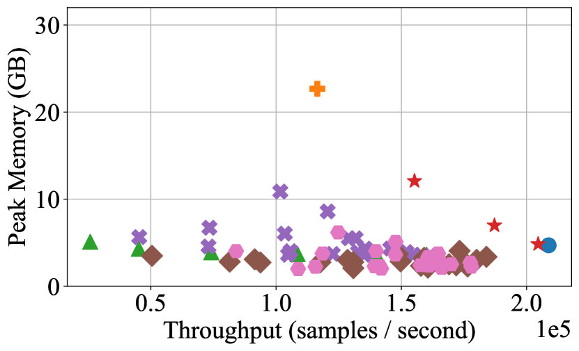
(a) MLP 1B, batch size 65536

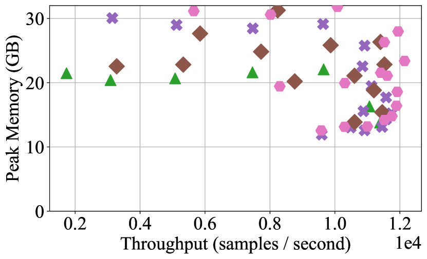
(b) MLP 17B, batch size 65536

(c) MLP 103B, batch size 256

Figure 5: Peak per-device memory vs throughput for MLP training models with fixed batch sizes across different distribution strategies as measured in simulation. The optimal strategy varies for each model and batch size.

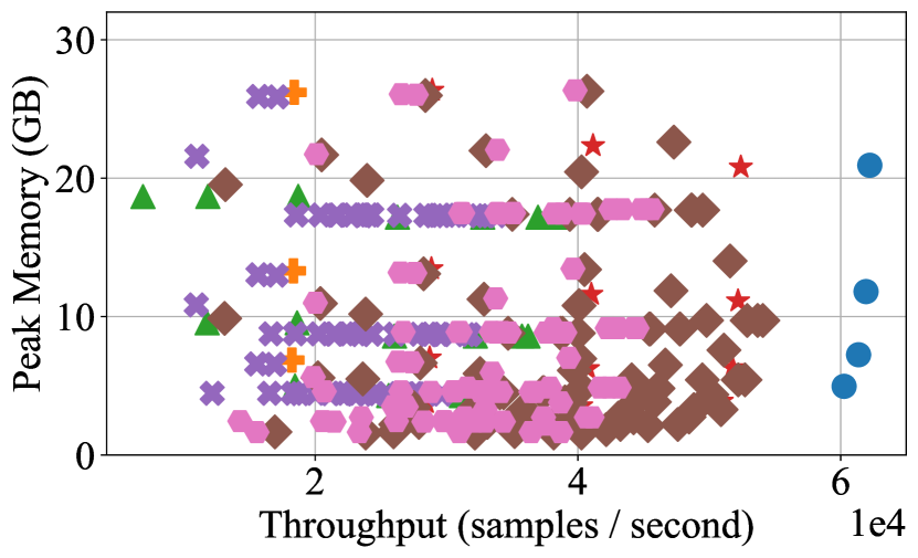
(a) GPT-2 1.6B

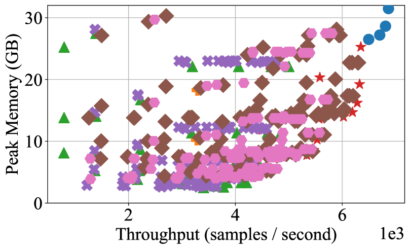
(b) GPT-2 13B

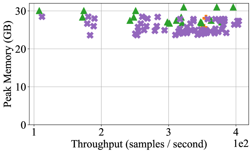
(c) GPT-2 175B

Figure 6: Peak per-device memory vs throughput for GPT-2 inference models across different distribution strategies as measured in simulation. Data includes all power-of-two batch sizes between 128 and 1048576. The optimal strategy varies for each model size.

5.2 Automated Distribution

In this section, we aim to validate DistIR’s ability to automatically identify efficient distribution strategies, and compare the optimization overhead to manual search on real hardware. We find that DistIR discovers high-performance strategies across both training and inference workloads while significantly lowering the optimization cost.

Setup.

We take the full search space of distributed configurations from §5.1 and then filter out configurations that are expected to exceed the 32-GB per GPU memory limit. From the remaining list, we simulate each strategy with DistIR to predict its performance, and execute the top 10 configurations in terms of predicted performance on the 16-GPU DGX node with the DistIR PyTorch backend.

As a baseline, we manually execute each model and batch size configuration with each pure distribution strategy (that is, pure data, tensor-model, and pipeline parallelism). For pipeline parallelism, we fix 128 microbatches according to a domain expert’s recommended heuristic of setting $K=8P$ ($K$ = microbatches, $P$ = pipeline stages) to minimize pipeline bubbles.

Results.

Tables 2 and 3 present the results for MLP training and GPT-2 inference respectively. For each model size, and batch size for training, we report the best performance achieved by each of the baseline distribution strategies as well as the strategies selected by the grid search. We observe that for all model size and batch size configurations, the strategies discovered by the grid search match or even exceed the performance of the baseline configurations. Moreover, the DistIR simulator is able to find these strategies far quicker than manual search on physical hardware. Table 1 details the end-to-end optimization time using DistIR vs exhaustively running all configurations for each model on the DGX. We see that optimization via simulation with DistIR is an order of magnitude faster for certain model sizes. This confirms that DistIR can effectively use simulation to drive efficient automatic optimization.

Model	Batch size	Best Config ($D$ / $T$ / $P$ / $K$)	vs D	vs T	vs P
MLP 1B	128	1 / 16 / 1 / 1	7.5$\times$	1.1$\times$	21.7$\times$
	256	1 / 16 / 1 / 1	6.3$\times$	1.1$\times$	21.2$\times$
	512	1 / 16 / 1 / 1	4.1$\times$	1.0$\times$	12.9$\times$
	1024	1 / 16 / 1 / 1	2.9$\times$	1.0$\times$	9.5$\times$
	2048	2 / 8 / 1 / 1	2.2$\times$	1.2$\times$	7.2$\times$
	4096	4 / 4 / 1 / 1	1.7$\times$	1.4$\times$	5.1$\times$
	8192	4 / 4 / 1 / 1	1.3$\times$	1.6$\times$	3.6$\times$
	16384	8 / 2 / 1 / 1	1.1$\times$	1.9$\times$	2.7$\times$
	32768	8 / 2 / 1 / 1	1.0$\times$	2.1$\times$	2.3$\times$
	65536	16 / 1 / 1 / 1	1.0$\times$	-	2.3$\times$
	131072	16 / 1 / 1 / 1	1.0$\times$	-	2.4$\times$
	262144	16 / 1 / 1 / 1	1.0$\times$	-	2.4$\times$
MLP 17B	128	1 / 16 / 1 / 1	-	1.1$\times$	43.8$\times$
	256	1 / 16 / 1 / 1	-	1.0$\times$	35.3$\times$
	512	1 / 16 / 1 / 1	-	1.0$\times$	22.4$\times$
	1024	1 / 16 / 1 / 1	-	1.0$\times$	15.6$\times$
	2048	1 / 16 / 1 / 1	-	1.0$\times$	10.0$\times$
	4096	2 / 8 / 1 / 1	-	1.1$\times$	6.1$\times$
	8192	4 / 4 / 1 / 1	-	1.2$\times$	3.7$\times$
	16384	4 / 4 / 1 / 1	-	-	2.4$\times$
	32768	2 / 4 / 2 / 8	-	-	1.5$\times$
	65536	4 / 2 / 2 / 8	-	-	1.3$\times$
	131072	4 / 2 / 2 / 32	-	-	-
MLP 103B	128	1 / 16 / 1 / 1	-	1.0$\times$	61.7$\times$
	256	1 / 16 / 1 / 1	-	1.0$\times$	-
	512	1 / 16 / 1 / 1	-	1.0$\times$	-
	1024	1 / 16 / 1 / 1	-	1.0$\times$	-

Table 2: The best distribution configuration, as predicted by the DistIR grid search, for each MLP training model and batch size. We also report the speedup in throughput of this configuration against pure data, tensor-model, and pipeline parallelism baselines on physical hardware. Note that it matches or exceeds the performance of the baselines in all cases.

Model	Best Config (Batch size / $D$ / $T$ / $P$ / $K$)	vs D	vs T	vs P
GPT-2 1.6B	32768 / 16 / 1 / 1 / 1	1.0$\times$	3.7$\times$	2.9$\times$
GPT-2 13B	16384 / 16 / 1 / 1 / 1	1.0$\times$	2.6$\times$	2.0$\times$
GPT-2 175B	1024 / 1 / 8 / 2 / 2	-	1.3$\times$	5.6$\times$

Table 3: The best distribution configuration, as predicted by the DistIR grid search, for each GPT-2 inference model size and its throughput speedup versus pure data, tensor-model, and pipeline parallelism baselines on physical hardware. The top pure baseline configurations were chosen by running all batch sizes that fit in memory starting from 128. The grid search configuration matches or exceeds the performance of the pure baselines in all cases.

5.3 Simulator Accuracy

DistIR’s simulator aims to to accurately rank the performance of distributed configurations on physical hardware. To measure this accuracy, we first randomly sample 70+ distributed configurations from the same space as in §5.1 for each of the 6 model architectures and execute these configurations on the DGX using the DistIR PyTorch backend. We then compare the simulated throughput with the throughput measured on real hardware. We also compute the Spearman correlation coefficient Spearman (1961) between the simulated and real throughput values; this value captures the similarity in ranking order between two variables, so we can apply it here to determine the effectiveness of DistIR’s ranking methodology.

Table 4 presents the results. We observe strong correlation for both MLP training and GPT-2 inference for all model sizes. However, there are still gaps between the absolute throughput values measured in simulation vs on physical hardware (see Figure 10 in the Appendix for more details). We attribute these discrepancies to the fact that we only use regression-based cost functions for few ops and use heuristics for the rest (§4); future work will include using profiled costs to improve raw throughput prediction accuracy.

Furthermore, our memory estimation is sometimes inaccurate because our backend allocates memory naively when needed, which leads to fragmentation and out-of-memory errors for configurations that the simulator predicts will fit on the device. Since DistIR determines all ops and their schedule explicitly, standard ahead-of-time allocation strategies would avoid such fragmentation.

Model	$N$	Correlation
		$r$	$p$
MLP 1B	94	.97	$<10^{-56}$
MLP 17B	94	.98	$<10^{-62}$
MLP 103B	71	.99	$<10^{-64}$
GPT-2 1.6B	94	.98	$<10^{-62}$
GPT-2 13B	75	.94	$<10^{-34}$
GPT-2 175B	78	.84	$<10^{-21}$

Table 4: Spearman correlation coefficients as a measure of simulator ranking accuracy. Configurations were selected uniformly randomly from the simulated grid search results and then run on the 16-GPU DGX node.

5.4 Simulator Scalability

A key property of DistIR is that it enables fast simulation, because all scheduling decisions are directly embedded in the IR. In this section, we test this claim in practice.

Figure 7 demonstrates how the DistIR simulator scales with respect to the program op count. We measure the wall clock execution time taken to simulate a sample of distributed GPT-2 models drawn from the search space in §5.1 and observe linear scaling as a function of the op count.

We note that the raw simulation times would improve significantly from a compiled (e.g. C++) implementation, but this is orthogonal to our core contributions.

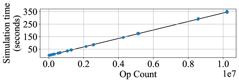
Figure 7: Scaling behavior of DistIR simulator. We observe linear scaling with respect to the program op count.

6 Related Work

Eager Frameworks.

Many existing libraries for distributed DNNs Narayanan et al. (2019); Shoeybi et al. (2019); Rasley et al. (2020) are implemented in eager frameworks such as PyTorch Paszke et al. (2019) that lack an IR. They allow unpredictable dynamic behavior which makes it extremely difficult to write analyses such as a general-purpose simulator. PipeDream Narayanan et al. (2019) uses cost models to optimize the partitioning of a model, but these are specific to their pipeline-parallel strategy.

SPMD IRs.

Graph-based frameworks such as XLA Leary & Wang (2017) and ONNX Runtime Microsoft have IRs that have been extended to represent distributed computation Yu et al. (2018); Huang et al. (2019); Lepikhin et al. (2021); Fedus et al. (2021); Xu et al. (2021). These works use the single-program-multiple-data (SPMD) methodology, because it provides concise representations of common data-parallel programs. In DistIR, we can outline such repetitive blocks of code into functions to reduce IR size (so far we have not needed to, see §5.4). On the other hand, as discussed in §2, SPMD-based frameworks have trouble representing pipeline parallelism within the IR.

Other IRs.

PartIR Vytiniotis et al. (2020) is an IR for partitioning tensor programs that is useful for high-level transformations, but the distribution (mapping of computation blocks to devices) is determined by a later lowering step. One could import the lowered program into DistIR in order to integrate with our simulator.

DaCe Ben-Nun et al. (2019), Lift Steuwer et al. (2017), and Elevate Hagedorn et al. (2020) all propose IRs for representing parallel computation. However, these IRs are primarily designed for maximizing single-node parallelism rather than optimizing distributed performance for large-scale DNNs. Halide Ragan-Kelley et al. (2017) separates what is computed from how it is computed; we plan to investigate integrating Halide’s approach in DistIR in order to make transforms more modular. TVM Chen et al. (2018) is an end-to-end optimizing compiler for DNNs, but to our knowledge it does not consider distribution.

DNN profiling and simulation.

DayDream Zhu et al. (2020) and DNNMem Gao et al. (2020) propose profiler-based simulators to accurately predict DNN execution time and memory respectively. However, DayDream has a fixed set of primitives for expressing optimizations and DNNMem operates over front-end model specifications, while we capture both model and distribution in a generic IR. FlexFlow Jia et al. (2019b) uses a simulator to search over a fixed strategy space but does not consider pipeline parallelism. Similarly, PipeDream-2BW Narayanan et al. (2020) includes a profiler to predict performance for various pipeline-parallel configurations but does not consider horizontal parallelism. DistIR’s simulator is more general as it is not tied to a particular class of models or strategies.

7 Future Work

There are three promising directions for future work.

First, one can upgrade our grid search to more sophisticated algorithms for automatic distribution, such as MCMC search Jia et al. (2019b), integer and dynamic programming Narayanan et al. (2019); Tarnawski et al. (2020), reinforcement learning Wang et al. (2020); Mirhoseini et al. (2017), and custom algorithms Narayanan et al. (2020); Jia et al. (2019a). Most of these are complementary to DistIR, as we can use DistIR’s simulator as their cost functions, and we plan to investigate these.

Second, we plan to integrate DistIR with popular distribution frameworks in order to support more DNN models and distribution strategies. The quick option is to use DistIR as shown in §5 to predict the best distributed configuration $(D,T,P,K)$, and feed that to, e.g., DeepSpeed Rasley et al. (2020), for execution. However, one would have to do extra work to make sure that the transforms implemented in DistIR stay in sync with the transforms implemented in DeepSpeed for the predictions to remain optimal. Alternatively, IR-based frameworks such as Jax/XLA can adopt DistIR as their representation of distribution. This would require porting the distribution strategies to be DistIR transforms, but this can potentially simplify their implementation as the lowering pass can be reused. In either case, one must empirically tune the cost models (as shown in §4) so that the simulator matches the backend.

Finally, we can improve our simulator’s runtime and memory estimations. Runtime estimation can be improved by extending empirical op cost models (§4) for all ops, and by using test inputs that correspond to input shapes seen during execution of real models. We can improve memory estimation by accounting for the temporary memory used by each op during its execution, which can be estimated empirically or analytically for ops with known kernels.

8 Conclusion

DistIR is an efficient IR for explicit representation of distributed DNN computation. DistIR permits efficient static analyses such as simulation that accelerate manual distribution as well as enable automatic distribution via search algorithms. Expressing distribution as transformations over DistIR functions allows one to develop hybrid strategies via composition of existing strategies. We demonstrate how DistIR can be used to facilitate automatic distribution by finding optimal strategies for large models among a hybrid space of distributions.

Appendix A Appendix

A.1 Expressivity Examples

⬇

1

2func @mlp_GradientCheckpointing(

3 %w1: D1,

4 %w2: D1,

5 %x: D1,

6 %y: D1) {

7 %as_f: D1 = @dense(%w1, %x)

8 %p: D1 = @dense(%w2, %as_f)

9 // Memory for %as_1 is reclaimed

10 %dp: D1 = @lossGrad(%p, %y)

11 // Recompute activation

12 %as_b: D1 = @dense(%w1, %x)

13 %dw2, %das: D1 = @denseGrad(%w2, %as_b, %dp)

14 %dw1, _: D1 = @denseGrad(%w1, %x, %das)

15 // Weight update (WU)

16 %w1_new: D1 = Optimizer(%w1, %dw1)

17 %w2_new: D1 = Optimizer(%w2, %dw2)

18 return %w1_new, %w2_new

19 }

20}

Figure 8: DistIR code listing for sequential training of a 2-layer MLP model using gradient checkpointing Chen et al. (2016).

⬇

1

2func @mlpDP_ZeRO(

3 %w1: D1,

4 %w2: D2,

5 %x_1: D1,

6 %x_2: D2,

7 %y_1: D1,

8 %y_2: D2) {

9 %as_1: D1 = @dense(%w1, %x_1)

10 // %w1 is managed exclusively by device 1

11 %w1_2_f: D2 = Send(%w1, 2)

12 %as_2: D2 = @dense(%w1_2_f, %x_2)

13 // Memory for %w1_2_f is reclaimed

14 // %w2 is managed exclusively by device 2

15 %w2_1_f: D1 = Send(%w2, 1)

16 %p_1: D1 = @dense(%w2_1_f, %as_1)

17 // Memory for %w2_1_f is reclaimed

18 %p_2: D2 = @dense(%w2, %as_2)

19 %dp_1: D1 = @lossGrad(%p_1, %y_1)

20 %dp_2: D2 = @lossGrad(%p_2, %y_2)

21 // %w2_1_f has been freed, so re-send %w2

22 %w2_1_b: D1 = Send(%w2, 1)

23 %dw2_1, %das_1: D1 = @denseGrad(%w2_1_b, %as_1, %dp_1)

24 %dw2_2, %das_2: D2 = @denseGrad(%w2, %as_2, %dp_2)

25 %dw1_1, _: D1 = @denseGrad(%w1, %x_1, %das_1)

26 // %w1_2_f has been freed, so re-send %w1

27 %w1_2_b: D2 = Send(%w1, 2)

28 %dw1_2, _: D2 = @denseGrad(%w1_2_b, %x_2, %das_2)

29 // Weight update (WU)

30 %dw1: D1 = MPIReduce([%dw1_1, %dw1_2], 1)

31 %dw2: D2 = MPIReduce([%dw2_1, %dw2_2], 2)

32 %w1_new: D1 = Optimizer(%w1, %dw1)

33 %w2_new: D2 = Optimizer(%w2, %dw2)

34 return %w1_new, %w2_new

35 }

36}

Figure 9: DistIR code listing for data-parallel training of a 2-layer MLP model over 2 devices with ZeRO-style parameter and gradient partitioning (ZeRO stages 2 and 3) Rajbhandari et al. (2019).

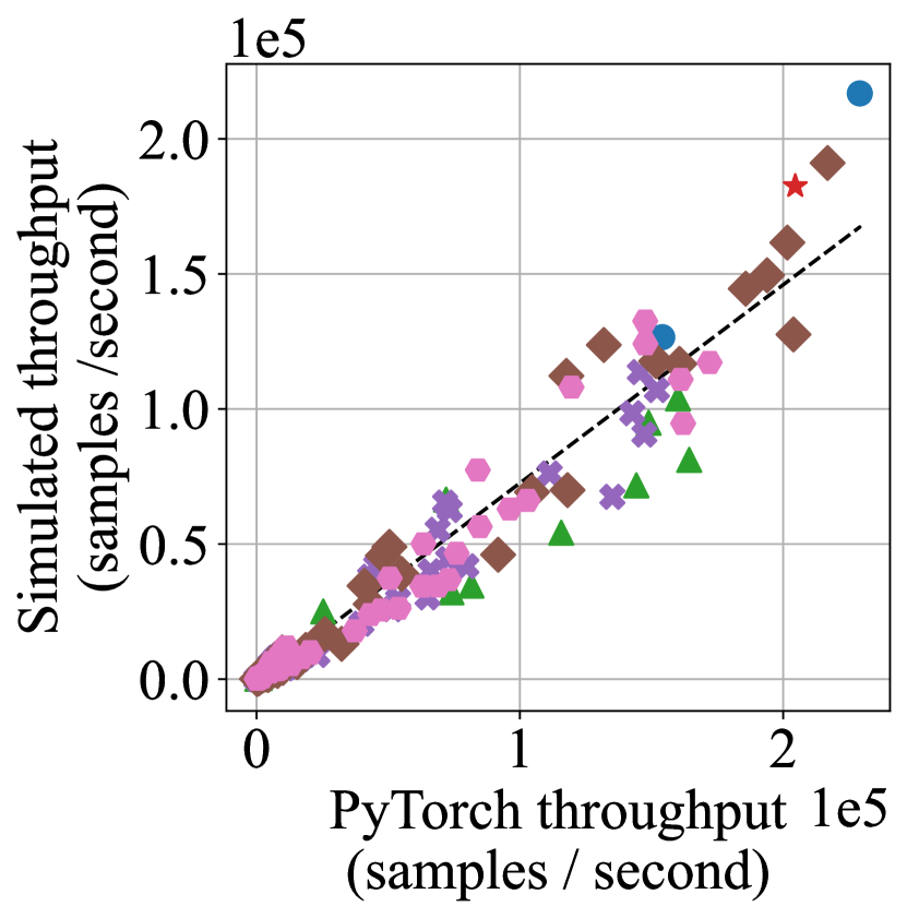
(a) MLP training.

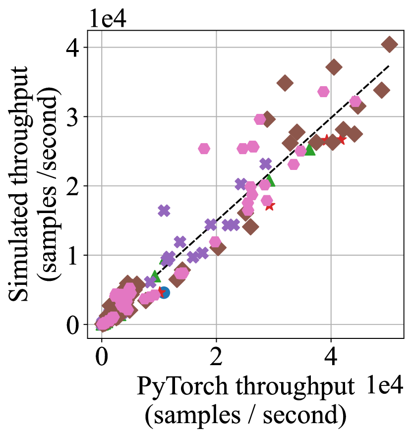
(b) GPT-2 inference.

Figure 10: Simulated performance predicted by the DistIR simulator vs real performance measured by the DistIR backend.

In this section we provide additional examples to highlight DistIR’s expressivity. In particular, Figure 8 demonstrates gradient checkpointing Chen et al. (2016) and Figure 9 demonstrates ZeRO partitioning Rajbhandari et al. (2019).

Gradient checkpointing is a memory-saving optimization which entails temporarily discarding activations in the forward pass after certain checkpoint nodes have finished executing (thereby reclaiming their memory) and then re-computing these activations in the backward pass when they are needed to compute the relevant gradients. This improves upon the default memory usage pattern which keeps all activations in device memory throughout the entire duration of the forward pass. Figure 8 presents an example of gradient checkpointing using DistIR. In this program, the first activation ($as_{f}$) is discarded after line 8 and is then re-computed at line 12 in the backward pass ($as_{b}$).

The ZeRO partitioning algorithms eliminate redundant memory usage in data-parallel training by distributing optimizer state (stage 1), gradients (stage 2), and parameters (stage 3) across nodes. Figure 9 provides an example of ZeRO stages 2 and 3 in a DistIR program. In this example, $w_{1}$ and its gradient are assigned exclusively to device 1, while $w_{2}$ and its gradient are assigned exclusively to device 2. Therefore $w_{1}$ must be sent to device 2 in line 11 so that device 2 can execute the first dense layer. Similarly $w_{2}$ must be sent to device 1 in line 15 for executing the second dense layer. The MPIReduce calls on lines 30 and 31 aggregate the gradients for $w_{1}$ and $w_{2}$ on devices 1 and 2 respectively.

A.2 Simulator Accuracy

Figure 10 compares the real throughput achieved by distributed MLP and GPT-2 configurations using the DistIR backend against the throughput predicted by the DistIR simulator for the same configurations. We generally find that the simulator produces accurate predictions of raw throughput, but there are cases where the error is more pronounced. As discussed in Section 5.3, we attribute these cases to the current lack of profiled op costs. Furthermore, we observe that distributed configurations involving pipeline parallelism tend to incur more prediction error; we suspect this is a result of the non-uniform communication patterns inherent to pipeline parallel execution. More fine-grained profiling could mitigate such discrepancies.

References

- Abadi et al. (2016) Abadi, M., Barham, P., Chen, J., Chen, Z., Davis, A., Dean, J., Devin, M., Ghemawat, S., Irving, G., Isard, M., et al. TensorFlow: A System for Large-Scale Machine Learning. In 12th USENIX Symposium on Operating Systems Design and Implementation (OSDI 16), pp. 265–283, 2016.
- Ben-Nun et al. (2019) Ben-Nun, T., de Fine Licht, J., Ziogas, A. N., Schneider, T., and Hoefler, T. Stateful Dataflow Multigraphs: A Data-Centric Model for Performance Portability on Heterogeneous Architectures. In Proceedings of the International Conference for High Performance Computing, Networking, Storage and Analysis, pp. 1–14, 2019.
- Bradbury et al. (2018) Bradbury, J., Frostig, R., Hawkins, P., Johnson, M. J., Leary, C., Maclaurin, D., Necula, G., Paszke, A., VanderPlas, J., Wanderman-Milne, S., and Zhang, Q. JAX: composable transformations of Python+NumPy programs, 2018. URL http://github.com/google/jax.
- Brown et al. (2020) Brown, T., Mann, B., Ryder, N., Subbiah, M., Kaplan, J. D., Dhariwal, P., Neelakantan, A., Shyam, P., Sastry, G., Askell, A., Agarwal, S., Herbert-Voss, A., Krueger, G., Henighan, T., Child, R., Ramesh, A., Ziegler, D., Wu, J., Winter, C., Hesse, C., Chen, M., Sigler, E., Litwin, M., Gray, S., Chess, B., Clark, J., Berner, C., McCandlish, S., Radford, A., Sutskever, I., and Amodei, D. Language Models are Few-Shot Learners. In Larochelle, H., Ranzato, M., Hadsell, R., Balcan, M. F., and Lin, H. (eds.), Advances in Neural Information Processing Systems, volume 33, pp. 1877–1901. Curran Associates, Inc., 2020. URL https://proceedings.neurips.cc/paper/2020/file/1457c0d6bfcb4967418bfb8ac142f64a-Paper.pdf.
- Chen et al. (2016) Chen, T., Xu, B., Zhang, C., and Guestrin, C. Training Deep Nets with Sublinear Memory Cost. arXiv preprint arXiv:1604.06174, 2016.
- Chen et al. (2018) Chen, T., Moreau, T., Jiang, Z., Zheng, L., Yan, E., Shen, H., Cowan, M., Wang, L., Hu, Y., Ceze, L., et al. TVM: An Automated End-to-End Optimizing Compiler for Deep Learning. In 13th USENIX Symposium on Operating Systems Design and Implementation (OSDI 18), pp. 578–594, 2018.
- Chen et al. (2012) Chen, X., Eversole, A., Li, G., Yu, D., and Seide, F. Pipelined back-propagation for context-dependent deep neural networks. In Thirteenth Annual Conference of the International Speech Communication Association, 2012.
- Cousot & Cousot (1977) Cousot, P. and Cousot, R. Abstract Interpretation: a Unified Lattice Model for Static Analysis of Programs by Construction or Approximation of Fixpoints. In Proceedings of the 4th ACM SIGACT-SIGPLAN Symposium on Principles of Programming Languages, pp. 238–252, 1977.
- Cousot & Cousot (1979) Cousot, P. and Cousot, R. Systematic design of program analysis frameworks. In Proceedings of the 6th ACM SIGACT-SIGPLAN symposium on Principles of programming languages, pp. 269–282, 1979.
- Dean et al. (2012) Dean, J., Corrado, G., Monga, R., Chen, K., Devin, M., Mao, M., Ranzato, M., Senior, A., Tucker, P., Yang, K., et al. Large Scale Distributed Deep Networks. In Advances in Neural Information Processing Systems, pp. 1223–1231, 2012.
- Fedus et al. (2021) Fedus, W., Zoph, B., and Shazeer, N. Switch Transformers: Scaling to Trillion Parameter Models with Simple and Efficient Sparsity. arXiv preprint arXiv:2101.03961, 2021.
- Gao et al. (2020) Gao, Y., Liu, Y., Zhang, H., Li, Z., Zhu, Y., Lin, H., and Yang, M. Estimating GPU Memory Consumption of Deep Learning Models. In Proceedings of the 28th ACM Joint Meeting on European Software Engineering Conference and Symposium on the Foundations of Software Egineering, pp. 1342–1352, 2020.
- Gaunt et al. (2017) Gaunt, A. L., Johnson, M. A., Riechert, M., Tarlow, D., Tomioka, R., Vytiniotis, D., and Webster, S. AMPNet: Asynchronous model-parallel training for dynamic neural networks. arXiv preprint arXiv:1705.09786, 2017.
- Hagedorn et al. (2020) Hagedorn, B., Lenfers, J., Koehler, T., Gorlatch, S., and Steuwer, M. A Language for Describing Optimization Strategies. arXiv preprint arXiv:2002.02268, 2020.
- Huang et al. (2019) Huang, Y., Cheng, Y., Bapna, A., Firat, O., Chen, D., Chen, M., Lee, H., Ngiam, J., Le, Q. V., Wu, Y., et al. GPipe: Efficient Training of Giant Neural Networks using Pipeline Parallelism. In Advances in Neural Information Processing Systems, pp. 103–112, 2019.
- Jia et al. (2019a) Jia, Z., Padon, O., Thomas, J., Warszawski, T., Zaharia, M., and Aiken, A. TASO: Optimizing Deep Learning Computation with Automatic Generation of Graph Substitutions. In Proceedings of the 27th ACM Symposium on Operating Systems Principles, pp. 47–62, 2019a.
- Jia et al. (2019b) Jia, Z., Zaharia, M., and Aiken, A. Beyond Data and Model Parallelism for Deep Neural Networks. In Talwalkar, A., Smith, V., and Zaharia, M. (eds.), Proceedings of Machine Learning and Systems, volume 1, pp. 1–13, 2019b. URL https://proceedings.mlsys.org/paper/2019/file/c74d97b01eae257e44aa9d5bade97baf-Paper.pdf.
- Krizhevsky (2014) Krizhevsky, A. One Weird Trick for Parallelizing Convolutional Neural Networks. arXiv preprint arXiv:1404.5997, 2014.
- Leary & Wang (2017) Leary, C. and Wang, T. XLA: TensorFlow, compiled. TensorFlow Dev Summit, 2017.
- Lepikhin et al. (2021) Lepikhin, D., Lee, H., Xu, Y., Chen, D., Firat, O., Huang, Y., Krikun, M., Shazeer, N., and Chen, Z. GShard: Scaling Giant Models with Conditional Computation and Automatic Sharding. In International Conference on Learning Representations, 2021. URL https://openreview.net/forum?id=qrwe7XHTmYb.
- (21) Microsoft. ONNX Runtime. URL https://microsoft.github.io/onnxruntime/.
- Mirhoseini et al. (2017) Mirhoseini, A., Pham, H., Le, Q. V., Steiner, B., Larsen, R., Zhou, Y., Kumar, N., Norouzi, M., Bengio, S., and Dean, J. Device placement optimization with reinforcement learning. In International Conference on Machine Learning, pp. 2430–2439. PMLR, 2017.
- Narayanan et al. (2019) Narayanan, D., Harlap, A., Phanishayee, A., Seshadri, V., Devanur, N. R., Ganger, G. R., Gibbons, P. B., and Zaharia, M. PipeDream: Generalized Pipeline Parallelism for DNN Training. In Proceedings of the 27th ACM Symposium on Operating Systems Principles, pp. 1–15, 2019.
- Narayanan et al. (2020) Narayanan, D., Phanishayee, A., Shi, K., Chen, X., and Zaharia, M. Memory-Efficient Pipeline-Parallel DNN Training. arXiv preprint arXiv:2006.09503, 2020.
- Narayanan et al. (2021) Narayanan, D., Shoeybi, M., Casper, J., LeGresley, P., Patwary, M., Korthikanti, V. A., Vainbrand, D., Kashinkunti, P., Bernauer, J., Catanzaro, B., et al. Efficient Large-Scale Language Model Training on GPU Clusters. arXiv preprint arXiv:2104.04473, 2021.
- (26) ONNX. Open neural network exchange (ONNX). URL https://onnx.ai/.
- Paszke et al. (2019) Paszke, A., Gross, S., Massa, F., Lerer, A., Bradbury, J., Chanan, G., Killeen, T., Lin, Z., Gimelshein, N., Antiga, L., et al. PyTorch: An Imperative Style, High-Performance Deep Learning Library. In Advances in Neural Information Processing Systems, pp. 8026–8037, 2019.
- Raffel et al. (2020) Raffel, C., Shazeer, N., Roberts, A., Lee, K., Narang, S., Matena, M., Zhou, Y., Li, W., and Liu, P. J. Exploring the Limits of Transfer Learning with a Unified Text-to-Text Transformer. Journal of Machine Learning Research, 21:1–67, 2020.
- Ragan-Kelley et al. (2017) Ragan-Kelley, J., Adams, A., Sharlet, D., Barnes, C., Paris, S., Levoy, M., Amarasinghe, S., and Durand, F. Halide: Decoupling Algorithms from Schedules for High-performance Image Processing. Communications of the ACM, 61(1):106–115, 2017.
- Rajbhandari et al. (2019) Rajbhandari, S., Rasley, J., Ruwase, O., and He, Y. ZeRO: Memory Optimization towards Training a Trillion Parameter Models. arXiv preprint arXiv:1910.02054, 2019.
- Rasley et al. (2020) Rasley, J., Rajbhandari, S., Ruwase, O., and He, Y. DeepSpeed: System Optimizations Enable Training Deep Learning Models with Over 100 Billion Parameters. In Proceedings of the 26th ACM SIGKDD International Conference on Knowledge Discovery & Data Mining, pp. 3505–3506, 2020.
- Shoeybi et al. (2019) Shoeybi, M., Patwary, M., Puri, R., LeGresley, P., Casper, J., and Catanzaro, B. Megatron-LM: Training Multi-Billion Parameter Language Models Using GPU Model Parallelism. arXiv preprint arXiv:1909.08053, 2019.
- Spearman (1961) Spearman, C. The Proof and Measurement of Association Between Two Things. 1961.
- Steuwer et al. (2017) Steuwer, M., Remmelg, T., and Dubach, C. Lift: a Functional Data-Parallel IR for High-Performance GPU Code Generation. In 2017 IEEE/ACM International Symposium on Code Generation and Optimization (CGO), pp. 74–85. IEEE, 2017.
- Tarnawski et al. (2020) Tarnawski, J. M., Phanishayee, A., Devanur, N., Mahajan, D., and Nina Paravecino, F. Efficient Algorithms for Device Placement of DNN Graph Operators. Advances in Neural Information Processing Systems, 33, 2020.
- Vytiniotis et al. (2020) Vytiniotis, D., Grewe, D., Schaarschmidt, M., Molloy, J., Belov, D., Paszke, A., Maclaurin, D., and Vasilache, N. PartIR: declarative abstractions for tensor program partitioning. Invited talk at PPDP, 2020.
- Wang et al. (2020) Wang, S., Rong, Y., Fan, S., Zheng, Z., Diao, L., Long, G., Yang, J., Liu, X., and Lin, W. Auto-MAP: A DQN Framework for Exploring Distributed Execution Plans for DNN Workloads. arXiv preprint arXiv:2007.04069, 2020.
- Xu et al. (2021) Xu, Y., Lee, H., Chen, D., Hechtman, B., Huang, Y., Joshi, R., Krikun, M., Lepikhin, D., Ly, A., Maggioni, M., et al. GSPMD: General and scalable parallelization for ml computation graphs. arXiv preprint arXiv:2105.04663, 2021.
- Yu et al. (2018) Yu, Y., Abadi, M., Barham, P., Brevdo, E., Burrows, M., Davis, A., Dean, J., Ghemawat, S., Harley, T., Hawkins, P., et al. Dynamic Control Flow in Large-scale Machine Learning. In Proceedings of the Thirteenth EuroSys Conference, pp. 1–15, 2018.
- Zhu et al. (2020) Zhu, H., Phanishayee, A., and Pekhimenko, G. Daydream: Accurately estimating the efficacy of optimizations for DNN training. In 2020 USENIX Annual Technical Conference (USENIX ATC 20), pp. 337–352. USENIX Association, July 2020. ISBN 978-1-939133-14-4. URL https://www.usenix.org/conference/atc20/presentation/zhu-hongyu.