Efficient Data Compression for 3D Sparse TPC via Bicephalous Convolutional Autoencoder

Abstract

Real-time data collection and analysis in large experimental facilities present a great challenge across multiple domains, including high energy physics, nuclear physics, and cosmology. To address this, machine learning (ML)-based methods for real-time data compression have drawn significant attention. However, unlike natural image data, such as CIFAR and ImageNet that are relatively small-sized and continuous, scientific data often come in as three-dimensional ($\mathbf{3}$D) data volumes at high rates with high sparsity (many zeros) and non-Gaussian value distribution. This makes direct application of popular ML compression methods, as well as conventional data compression methods, suboptimal. To address these obstacles, this work introduces a dual-head autoencoder to resolve sparsity and regression simultaneously, called Bicephalous Convolutional AutoEncoder (BCAE). This method shows advantages both in compression fidelity and ratio compared to traditional data compression methods, such as MGARD, SZ, and ZFP. To achieve similar fidelity, the best performer among the traditional methods can reach only half the compression ratio of BCAE. Moreover, a thorough ablation study of the BCAE method shows that a dedicated segmentation decoder improves the reconstruction.

I Introduction

The super Pioneering High Energy Nuclear Interaction eXperiment (sPHENIX) at the Relativistic Heavy Ion Collider (RHIC) will perform high-precision measurements of jets and heavy-flavor observables for a wide selection of high energy nuclear collision systems, elucidating the microscopic nature of strongly interacting matter, ranging from nucleons to strongly coupled quark-gluon plasma [1]. As illustrated in Figure 1, a next-generation continuous readout time projection chamber (TPC) is the main tracking detector for sPHENIX. The overall sPHENIX experimental data rate is dominated by the TPC, which reads out at a rate of $O(1)$ Tbps and records at $O(100)$ Gbps to persistent storage [28]. Therefore, the experiment’s storage efficiency and throughput capability can directly benefit from high-fidelity compression algorithms optimized for the TPC data stream.

An autoencoder (AE) network is an effective method for data compression [17, 32]. Compared to traditional data reduction methods, such as principal component analysis [11] and Isomap [30], AE often results in a higher compression ratio and better reconstruction accuracy [10]. Conceptually, AE consists of two neural networks (NNs): an encoder and a decoder. The encoder maps a high-dimensional data block into low-dimensional compressed representations, while a decoder recreates the input data from the code. For image data with shift-invariance properties, a convolutional autoencoder (CAE) often is used. CAE uses a convolutional network [20, 19, 26, 14] as the encoder and a deconvolutional network [34, 35] as the decoder. Data compression is achieved by having a smaller bit length compared to input. Unlike other generative NN models, such as a variational autoencoder [18, 25, 31] or generative adversarial network (GAN) [12, 6], AE emphasizes faithful recreation of the original data point instead of the diversity of generated data. CAE is not without issues. Reconstructed images often are blurry and sometimes accompanied by checkerboard artifacts [24], which can be especially devastating for sparse data with sharp boundaries.

Figure 1: sPHENIX experiment with the TPC in yellow, simulated data with particle trajectories in TPC highlighted in red, and $13$ $\mu$s of TPC data presented in a $3$D data frame.

II Method

II-A Data Gathering and Preparation

We use simulated data for $200$ GeV Au$+$Au collisions detected by the sPHENIX TPC, which is generated based on the HIJING event generator [33] and Geant4 Monte Carlo detector simulation package [4] integrated with the sPHENIX software framework [27]. sPHENIX’s TPC continuously detects thousands of charged particles produced at high-energy Au$+$Au at RHIC, which collide at a rate of $O(100)$ kHz. The ionization charge produced by these particles in the TPC gas volume is drifted, amplified, and collected by $160$k mini pads [5] and digitized continuously using analog-digital converters (ADCs) inside of the SAMPA v5 application-specific integrated circuit at a rate of $20$ MHz [16, 28]. As the ionization charge drifts along the $z$ axis at $\sim 8$ cm$/\mu$s, the ADC time series can be translated to the $z$-location dependent ionization charge density. All ADC values are $10$-bit unsigned integers ($\in[0,1023]$), representing the charge density of the initial ionization. The trajectory location is interpolated between the location of neighboring pads using the ADC amplitude. Hence, in a lossy compression, it is important to preserve the relative ADC ratio between the pads. Before readout of the TPC data, the ADC values are zero-suppressed in the SAMPA chips. For this study, we assume a simple zero suppression as ADC$>64$ and set all ADC bins below this threshold to zero. The data streams from SAMPA chips are read out via $960$ $6$-Gbps optical fibers through the FELIX interfaces [8] to a fleet of commodity computing servers. The computing capability in the TPC readout path allows a compression algorithm to be applied in the field-programmable gate array in the FELIX interface or the computing servers. The detector’s TPC mini-pad array is composed of $48$ cylindrical layers that are grouped into the inner, middle, and outer layers, each with $16$ layers. Detectors in each layer can be unwrapped into a rectangular grid with rows in the $z$ direction and columns in the azimuthal direction. All layer groups have the same number of rows of detector pads but different numbers of columns. Each full three-dimensional ($\mathbf{3}$D) data volume of the outer layer group is in the shape of $(2304,498,16)$ in the azimuthal, horizontal, and radial orders. To match the segmentation of the TPC readout data concentrator, we divide a full frame into $12$ non-overlapping sections along the azimuth and halve the horizontal direction, resulting in the input data shape of $(192,249,16)$.

II-B Bicephalous Convolutional AutoEncoder (BCAE)

Figure 2: Summary of the BCAE architecture and the ResBlock. Our BCAE is composed of one encoder and two decoders. The decoders $D_{\textrm{s}}$ is designated to solve the segmentation problem. The combined output from $D_{\textrm{s}}$ and $D_{\textrm{r}}$ is used to solve the regression problem.

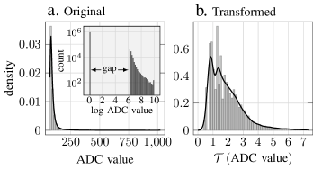
The long tail and sharp edge in the distribution of ADC values present a great challenge. Figure 3a inset shows the histogram in logarithmic scale of ADC values, revealing the sparsity and a gap between $0$ and $64$. NNs have difficulties with such distributions [3, 13], which we confirm in the ablation studies (Sec. III-C). We propose two techniques to solve the problem: 1) reforming the voxel-level regression into a segmentation (voxel-level binary classification) and a regression and 2) predicting a transform of the input data.

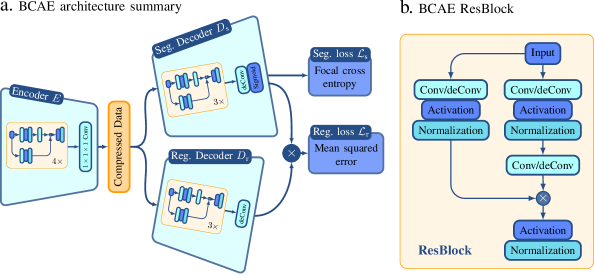
Bicephalous decoder: Figure 2a shows that our BCAE has two decoders, $D_{\textrm{s}}$ for voxel segmentation and $D_{\textrm{r}}$ for regression. From the compressed data, the segmentation decoder $D_{\textrm{s}}$ classifies each voxel into two categories: zero-valued or positive-valued. The output from $D_{\textrm{s}}$ is evaluated with the focal loss $\mathcal{L}_{\textrm{s}}$, which is designed to deal with an unbalanced data set [22]. The output from the regression decoder $D_{\textrm{r}}$ is combined with that from $D_{\textrm{s}}$ and evaluated with a mean squared error (MSE) loss $\mathcal{L}_{\textrm{r}}$.

Predicting a transformed input: To deal with the sharp edge in the input distribution induced by the zero suppression, $D_{\textrm{r}}$ does not predict an input ADC value, but rather its transform. The transform has the form: $\mathcal{T}(x)=\log(x-64)/6$, and let $x$ be a voxel with nonzero value $v_{x}$, $D_{\textrm{r}}$ approximates $\mathcal{T}(v_{x})$. To motivate the transform, we plot the histogram of raw and transformed nonzero ADC values in Figure 3a and b (for all ADC values, see the inset of a). It is evident that the transformed distribution better resembles a normal distribution. We borrow the idea of input transform from [3], where the technique is applied to an electron-proton scattering events simulation with GAN. As in [3], we do not transform the input before feeding it to the network. We assume the network’s output (more precisely, that of $D_{\textrm{r}}$) is an approximation for the transformed input. Before passing the prediction to the loss function, we apply the inverse transform $\mathcal{T}^{-1}$.

Figure 3: Motivation for input transformation. Panel a: histogram of nonzero ADC values; Panel b: histogram of $\mathcal{T}(\textrm{nonzero ADC values})$. The sharp edge around $64$ and long tail are resolved to an extent with the transform. The inset of Panel a shows the histogram in logarithmic scale of $\log_{2}(\cdot)$ ADC values, revealing the sparsity of nonzero values and a gap between $0$ and $64$.

Segmentation loss $\mathcal{L}_{\textrm{s}}$: Let $v_{x}$ be voxel $x$’s ADC value, and the log ADC value $v^{\prime}_{x}$ is defined to be $\log_{2}\left(v_{x}+1\right)$. Because a nonzero ADC value is $\geq 64$, the true class label of $x$ should be $0$ if $v^{\prime}_{x}<6$ or $1$ if otherwise. However, to make the loss function differentiable, we use the Sigmoid step function

$$\mathcal{S}(v;\mu,\alpha)=\left(1+\exp\left(-\alpha(v-\mu)\right)\right)^{-1}$$

to achieve a “soft classification” instead. The Sigmoid step function maps $v<\mu$ to a value close to $0$ and $v>\mu$, $1$. For this study, we set $\mu=6$ and $\alpha=20$. Let $\hat{l}_{x}$ be the output of $D_{\textrm{s}}$ for voxel $x$, and the focal loss is defined to be

$$\mathcal{L}_{\textrm{r}}\left(\left\{\left.\hat{l}_{x}\right|x\right\};\gamma\right)= \frac{1}{M}\sum_{x}-l_{x}\log_{2}\left(\hat{l}_{x}\right)\left(1-\hat{l}_{x}\right)^{\gamma}$$

$$-\left(1-l_{x}\right)\log_{2}\left(1-\hat{l}_{x}\right)\left(\hat{l}_{x}\right)^{\gamma},$$ (1)

where $M$ is the total number of voxels, $l_{x}$ is the soft label, and $\gamma$ is the focusing parameter. Focal loss is used because we have only $10\%$ of nonzero ADC values on average, and focal loss is shown to perform well when positive examples are relatively sparse. In this study, we set $\gamma=2$.

Regression loss $\mathcal{L}_{\textrm{r}}$: Denoted by $\hat{v}_{x}$ the prediction for voxel $x$ given by $D_{\textrm{r}}$, the combined prediction $\tilde{v}_{x}$ is defined as

$$\tilde{v}_{x}=\left\{\begin{array}[]{ll}\mathcal{T}^{-1}\left(\hat{v}_{x}\right),&\hat{l}_{x}\geq h,\\ 0,&\hat{l}_{x}<h,\end{array}\right.$$ (2)

where $h$ is a threshold and the regression loss $\mathcal{L}_{\textrm{r}}$ is defined as

$$\mathcal{L}_{\textrm{r}}\left(\left\{\left.\tilde{v}_{x},v_{x}\right|x\right\};h\right)=\frac{1}{M}\sum_{x}\left(\tilde{v}_{x}-v_{x}\right)^{2},$$ (3)

where $M$ is the total number of voxels.

Architectural details: BCAEs are constructed using the ResBlock in Figure 2b. The ResBlock design is inspired by the residual block proposed in [15]. However, unlike a residual block in [15] that preserves the input size, we downsample and upsample with ResBlock. On the main path of a ResBlock, we have (de)convolution, normalization, activation, and an additional (de)convolution layer. We downsample or upsample at the first (de)convolution layer and use kernel size $3$ and stride $1$ uniformly for the second. We also only increase or decrease the number of channels at the first (de)convolution layer on the main path while maintaining it at the second (de)convolution layer. The three layers on the ResBlock sidetrack are exactly the same as the first group of layers on the main path, and the encoder has four ResBlocks. The encoder has four ResBlocks and ends with a $1\times 1\times 1$ convolution layer with $8$ channels, while $D_{\textrm{s}}$ and $D_{\textrm{r}}$ have three ResBlocks plus a deconvolution layer as shown in Figure 2a. $D_{\textrm{s}}$ also has a Sigmoid layer to constrain output values between $0$ and $1$. For activation and normalization, we use leaky rectified linear activation function ReLU with negative slope $0.1$ and instance normalization.

Training: We implement the BCAE with PyTorch, using $960$ sections (see Sec. II-A) for training and $320$ for testing. We train the BCAE with batch size $32$ for $2000$ epochs. For the optimizer, we use the AdamW with $\beta_{1},\beta_{2}=0.9,0.999$ and $0.01$ weight decay. We set the initial learning rate to be $0.01$ and decrease it by $5\%$ every $20$ epochs. To match the magnitudes of $\mathcal{L}_{\textrm{s}}$ and $\mathcal{L}_{\textrm{r}}$, we use the following approach to combine the losses: let $\rho^{t}_{\textrm{s}}$ and $\rho^{t}_{\textrm{r}}$ be the segmentation and regression losses of epoch $t$. Then, the loss function at epoch $t+1$ is defined as $\mathcal{L}^{t+1}=\left(\rho^{t}_{\textrm{r}}/\rho^{t}_{\textrm{s}}\right)\mathcal{L}_{\textrm{s}}+\mathcal{L}_{\textrm{r}}$.

III Results

III-A BCAE Compression Ratio

The ADC values originally are $10$-bit integers saved as $16$-bit unsigned integers. BCAE runs with $32$-bit floats, and the compressed data output from the encoder as $32$-bit floats. To increase the compression ratio, we save the compressed data as $16$-bit floats. The decoders then can either run with half-precision ($16$-bit floats) or upcast the compression data to $32$-bit floats before running. As such, we can calculate BCAE’s compression ratio using only the input and output shapes. The input shape is $(1,192,249,16)$ (See Sec. II-A). The output shape is $(8,13,17,16)$. Hence, the compression ratio of BCAE equals $\left(1\times 192\times 249\times 16\right)/\left(8\times 13\times 17\times 16\right)=27.04$.

III-B Comparison with Three Existing Compression Algorithms

Figure 4: Relation between MSE and compression ratio.

Figure 5: Histogram of reconstructed ADC values for the four compression methods. To compare with BCAE at compression ratio $27$, we fix MGARD at ratio $27.05$, SZ at ratio $23.96$, and ZFP at ratio $19.26$. The reconstructed distribution of BCAE (Panel d) is closer to that of the ground truth than the other three methods at similar or smaller compression ratios. Both MGARD and ZFP have reconstructed values below zero, while SZ’s approximation is overly simplified and distorted. Of note, a spike on the high end (ADC$=1023$) is due to the $10$-bit limitation of the ADC chip, which outputs an overflow value with the max ADC number. BCAE decompressed value may exceed this instrumental limit.

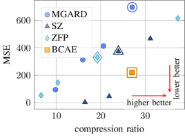
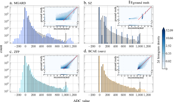
MGARD [7], or MultiGrid Adaptive Reduction of Data, is a technique for multilevel lossy compression of scientific data based on the theory of multigrid methods [2]. MGARD takes an $\ell_{\infty}$ error bound as the parameter, and the compression is successful if the maximum absolute difference between the raw and reconstructed values is below the bound. SZ [9, 29, 21] is an error-controlled lossy compression algorithm optimized for high-compression ratios. SZ provides five error-bounding modes, including absolute and relative errors and their combinations. ZFP [23] is a compressed format for representing two- ($2$) to four ($4$)-dimensional arrays that exhibit spatial correlation. ZFP provides three lossy compression modes: fixed-rate, fixed-precision, and fixed-accuracy. The fixed-accuracy mode is the same as the $\ell_{\infty}$ error-bound mode. ZFP requires padding to make dimensions a multiple of $4$. The compressed data of all three benchmarking algorithms are saved in binary, and their compression ratios are calculated as the averaged ratio of input size (as $16$-bit floats) to output file size. For comparison, we use the $\ell_{\infty}$ error-bound mode, which is provided by all three algorithms. Because the $\ell_{\infty}$ error bound does not offer direct control over compression ratio, we determine the relation between MSE and compression ratio by surveying a range of $\ell_{\infty}$ bounds for each algorithm. Specifically, for each $\ell_{\infty}$ bound, we run the algorithm on $100$ sampled $3$D sections then calculate the averaged compression ratios and MSEs.

To compare reconstruction distributions with BCAE at compression ratio $27$, we fix MGARD at ratio $27.05$, SZ at ratio $23.96$, and ZFP at ratio $19.26$. Figure 4 summarizes the results and shows that BCAE achieves a much lower MSE than benchmarking algorithms at similar compression ratios. We also demonstrate one ($1$)-dimensional and $2$D histograms in Figure 5. For $1$D histograms, we plot the ground truth distribution of ADC values in gray. Both MGARD and ZFP have reconstructed values below zero, while SZ’s approximation is overly simplified and distorted. Because of the gap in the ground truth distribution between $0$ and $64$, we can post-process the reconstructed values of MGARD, SZ, and ZFP by thresholding. Explicitly, we find a threshold $h$ and map each reconstructed value $<h$ to $0$ while keeping those $>h$ unchanged. The threshold values, $11$ for MGARD, $8$ for SZ, and $32$ for ZFP, are chosen to minimize the MSEs. We plot $2$D histograms after the post-processing on log ADC values. We omit the portions of $2$D histograms that represent the gap in the ground truth. We calculate the MSE, mean absolute error of log ADC value (log MAE), and Peak signal-to-noise ratio (PSNR) after the post-processing and record the results in Table I. All evaluations are done on raw ADC values.

TABLE I: Performance comparison

	Compr. ratio $\uparrow$	MSE $\downarrow$	log MAE $\,\downarrow$	PSNR$\uparrow$
MGARD	$\mathbf{27}$	$626.28$	$1.213$	$3.223$
SZ	$24$	$369.69$	$0.302$	$3.452$
ZFP	$19$	$219.48$	$0.267$	$3.678$
CAE	$27$	$227.61$	$0.349$	$3.703$
BCAEwoT	$27$	$230.59$	$0.193$	$3.706$
BCAE	$\mathbf{27}$	$\mathbf{218.44}$	$\mathbf{0.185}$	$\mathbf{3.724}$

III-C Ablation Study

Figure 6: Ablation study. We compare the BCAE to regression-only CAE and BCAE without transform (BCAEwoT). The reconstructed distribution of BCAE (Panel d) most closely resembles the ground truth distribution, and the reconstructed BCAE images (Panel h) also have the highest quality.

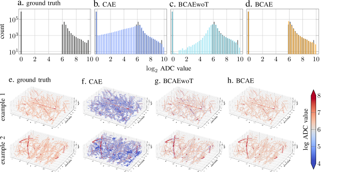
We compare the BCAE to regression-only CAE and BCAE without transform (BCAEwoT). BCAEwoT is obtained by adding a ReLU layer to $D_{\textrm{r}}$ of BCAE, and CAE is gleaned by removing $D_{\textrm{s}}$ from BCAEwoT. The combined prediction $\tilde{v}_{x}$ BCAEwoT determines for $x$ is

$$\tilde{v}_{x}=\left\{\begin{array}[]{ll}\hat{v}_{x},&\hat{l}_{x}\geq h,\\ 0,&\hat{l}_{x}<h.\end{array}\right.$$ (4)

In Figure 6a-d, we show the histograms of true log ADC values $v^{\prime}_{x}$ and reconstructed ones by CAE, BCAEwoT, and BCAE of 1 million sampled voxels. Figure 6b shows that CAE fills in the gap, meaning it significantly blends and blurs around the segmentation, which is confirmed by the $3$D visualization in Figure 6f. BCAEwoT approximates the input distribution better because a fraction of voxels with small ADC values are classified as zero. In Figure 6g, we see that BCAEwoT offers more clear-cut reconstructed images. Figure 6d shows that the reconstructed distribution of BCAE most closely resembles the original distribution, while reconstructed BCAE images (Figure 6h) also have the highest quality.

Because $D_{\textrm{s}}$ outputs a continuous value in $[0,1]$, we may adjust $h$ in Eq. (2) and (4) after training to decrease MSE further. Notably, with $h=.4$ for BCAEwoT and $h=.46$ for BCAE, we get the lowest respective MSEs on training data. Test results in Table I are obtained by applying the new thresholds instead of the $.5$ used in training. Furthermore, as the downstream application of TPC hit position determination focuses the ratios of ADC values between neighboring voxels, we also care about MAE in logarithmic scale of ADC values, where BCAE achieves the lowest score.

Conclusion

We have developed BCAE, a deep learning method for sparse ($\mathbf{3}$D) data compression. Compared to conventional compression methods, BCAE achieves higher fidelity and higher compression ratio. Yet, as with all deep learning methods, a trained BCAE model is data set specific and requires unsupervised training. We also demonstrate the effectiveness of our dual-head decoder design by conducting an ablation study that shows both logarithmic transform and dedicated segmentation decoder are important to match the ADC value distribution in logarithmic scale, which is critical in our application.

In the future, we want to integrate a differentiable proxy of sPHENIX downstream analysis criteria as part of the loss function to enable end-to-end training. In this way, the compression method becomes downstream task-aware and can better serve the overall scientific need. The segmentation decoder $D_{\textrm{s}}$ also can be trained with domain information to identify noise voxels. We expect BCAE can become a powerful tool that may sensitively preserve the signal voxel while filtering out the noise voxels in the raw data, which will improve the compression ratio and perform data reduction in a single set of algorithms.

References

- [1] A. Adare et al. An Upgrade Proposal from the PHENIX Collaboration. 1 2015.
- [2] Mark Ainsworth, Ozan Tugluk, Ben Whitney, and Scott Klasky. Multilevel techniques for compression and reduction of scientific data—the univariate case. Computing and Visualization in Science, 19(5-6):65–76, 2018.
- [3] Yasir Alanazi, Nobuo Sato, Tianbo Liu, W Melnitchouk, Michelle P Kuchera, Evan Pritchard, Michael Robertson, Ryan Strauss, Luisa Velasco, and Yaohang Li. Simulation of electron-proton scattering events by a feature-augmented and transformed generative adversarial network (fat-gan). arXiv preprint arXiv:2001.11103, 2020.
- [4] J. Allison et al. Recent developments in Geant4. Nucl. Instrum. Meth. A, 835:186–225, 2016.
- [5] B. Azmoun, P. Garg, T. K. Hemmick, M. Hohlmann, A. Kiselev, M. L. Purschke, C. Woody, and A. Zhang. Design Studies for a TPC Readout Plane Using Zigzag Patterns with Multistage GEM Detectors. IEEE Trans. Nucl. Sci., 65(7):1416–1423, 2018.
- [6] Andrew Brock, Jeff Donahue, and Karen Simonyan. Large scale GAN training for high fidelity natural image synthesis.
- [7] Jieyang Chen, Lipeng Wan, Xin Liang, Ben Whitney, Qing Liu, David Pugmire, Nicholas Thompson, Matthew Wolf, Todd Munson, Ian Foster, et al. Accelerating multigrid-based hierarchical scientific data refactoring on gpus. arXiv preprint arXiv:2007.04457, 2020.
- [8] Kai Chen, Hucheng Chen, Jin Huang, Francesco Lanni, Shaochun Tang, and Weihao Wu. A Generic High Bandwidth Data Acquisition Card for Physics Experiments. IEEE Trans. Instrum. Measur., 69(7):4569–4577, 2019.
- [9] Sheng Di and Franck Cappello. Fast error-bounded lossy hpc data compression with sz. In 2016 ieee international parallel and distributed processing symposium (ipdps), pages 730–739. IEEE, 2016.
- [10] Quentin Fournier and Daniel Aloise. Empirical comparison between autoencoders and traditional dimensionality reduction methods. In 2019 IEEE Second International Conference on Artificial Intelligence and Knowledge Engineering (AIKE), pages 211–214.
- [11] Karl Pearson F.R.S. LIII. on lines and planes of closest fit to systems of points in space. 2(11):559–572. Publisher: Taylor & Francis _eprint: https://doi.org/10.1080/14786440109462720.
- [12] Ian Goodfellow, Jean Pouget-Abadie, Mehdi Mirza, Bing Xu, David Warde-Farley, Sherjil Ozair, Aaron Courville, and Yoshua Bengio. Generative adversarial nets. In Z. Ghahramani, M. Welling, C. Cortes, N. D. Lawrence, and K. Q. Weinberger, editors, Advances in Neural Information Processing Systems 27, pages 2672–2680. Curran Associates, Inc.
- [13] Bobak Hashemi, Nick Amin, Kaustuv Datta, Dominick Olivito, and Maurizio Pierini. Lhc analysis-specific datasets with generative adversarial networks. arXiv e-prints, pages arXiv–1901, 2019.
- [14] Kaiming He, Xiangyu Zhang, Shaoqing Ren, and Jian Sun. Deep residual learning for image recognition. In 2016 IEEE Conference on Computer Vision and Pattern Recognition, CVPR 2016, Las Vegas, NV, USA, June 27-30, 2016, pages 770–778.
- [15] Kaiming He, Xiangyu Zhang, Shaoqing Ren, and Jian Sun. Deep residual learning for image recognition. In Proceedings of the IEEE conference on computer vision and pattern recognition, pages 770–778, 2016.
- [16] Hugo Hernández et al. A Monolithic 32-Channel Front End and DSP ASIC for Gaseous Detectors. IEEE Trans. Instrum. Measur., 69(6):2686–2697, 2019.
- [17] G. E. Hinton and R. R. Salakhutdinov. Reducing the dimensionality of data with neural networks. 313(5786):504–507. Publisher: American Association for the Advancement of Science Section: Report.
- [18] Diederik P. Kingma and Max Welling. Auto-encoding variational bayes.
- [19] Alex Krizhevsky, Ilya Sutskever, and Geoffrey E Hinton. ImageNet classification with deep convolutional neural networks. In F. Pereira, C. J. C. Burges, L. Bottou, and K. Q. Weinberger, editors, Advances in Neural Information Processing Systems 25, pages 1097–1105. Curran Associates, Inc.
- [20] Yann LeCun, Bernhard Boser, John S Denker, Donnie Henderson, Richard E Howard, Wayne Hubbard, and Lawrence D Jackel. Backpropagation applied to handwritten zip code recognition. 1(4):541–551. Publisher: MIT Press.
- [21] Xin Liang, Sheng Di, Dingwen Tao, Sihuan Li, Shaomeng Li, Hanqi Guo, Zizhong Chen, and Franck Cappello. Error-controlled lossy compression optimized for high compression ratios of scientific datasets. In 2018 IEEE International Conference on Big Data (Big Data), pages 438–447. IEEE, 2018.
- [22] Tsung-Yi Lin, Priya Goyal, Ross Girshick, Kaiming He, and Piotr Dollár. Focal loss for dense object detection. In Proceedings of the IEEE international conference on computer vision, pages 2980–2988, 2017.
- [23] Peter Lindstrom. Fixed-rate compressed floating-point arrays. IEEE transactions on visualization and computer graphics, 20(12):2674–2683, 2014.
- [24] Augustus Odena, Vincent Dumoulin, and Chris Olah. Deconvolution and checkerboard artifacts.
- [25] Ali Razavi, Aaron van den Oord, and Oriol Vinyals. Generating diverse high-fidelity images with vq-vae-2. In Advances in Neural Information Processing Systems, pages 14837–14847.
- [26] K. Simonyan and A. Zisserman. Very deep convolutional networks for large-scale image recognition.
- [27] sPHENIX. sphenix software repositories https://github.com/sphenix-collaboration. 2019.
- [28] sPHENIX. Technical design report: sphenix experiment at rhic. 2019.
- [29] Dingwen Tao, Sheng Di, Zizhong Chen, and Franck Cappello. Significantly improving lossy compression for scientific data sets based on multidimensional prediction and error-controlled quantization. In 2017 IEEE International Parallel and Distributed Processing Symposium (IPDPS), pages 1129–1139. IEEE, 2017.
- [30] Joshua B. Tenenbaum, Vin de Silva, and John C. Langford. A global geometric framework for nonlinear dimensionality reduction. 290(5500):2319–2323. Publisher: American Association for the Advancement of Science Section: Report.
- [31] Arash Vahdat and Jan Kautz. NVAE: A deep hierarchical variational autoencoder. In H. Larochelle, M. Ranzato, R. Hadsell, M. F. Balcan, and H. Lin, editors, Advances in Neural Information Processing Systems, volume 33, pages 19667–19679. Curran Associates, Inc.
- [32] Wei Wang, Yan Huang, Yizhou Wang, and Liang Wang. Generalized autoencoder: A neural network framework for dimensionality reduction. pages 490–497.
- [33] Xin-Nian Wang and Miklos Gyulassy. HIJING: A Monte Carlo model for multiple jet production in p p, p A and A A collisions. Phys. Rev. D, 44:3501–3516, 1991.
- [34] Matthew D. Zeiler, Dilip Krishnan, Graham W. Taylor, and Rob Fergus. Deconvolutional networks. In 2010 IEEE Computer Society Conference on Computer Vision and Pattern Recognition, pages 2528–2535. ISSN: 1063-6919.
- [35] Matthew D. Zeiler, Graham W. Taylor, and Rob Fergus. Adaptive deconvolutional networks for mid and high level feature learning. In 2011 International Conference on Computer Vision, pages 2018–2025. ISSN: 2380-7504.