Extracting the scaling dimension of quantum Hall quasiparticles from current correlations

Abstract

Fractional quantum Hall quasiparticles are generally characterized by two quantum numbers: electric charge $Q$ and scaling dimension $\Delta$. For the simplest states (such as the Laughlin series), the scaling dimension determines the quasiparticle’s anyonic statistics (the statistical phase $\theta=2\pi\Delta$). For more complicated states (featuring counterpropagating modes or non-Abelian statistics), knowing the scaling dimension is not enough to extract the quasiparticle statistics. Nevertheless, even in those cases, knowing the scaling dimension facilitates distinguishing different candidate theories for describing the quantum Hall state at a particular filling (such as PH-Pfaffian and anti-Pfaffian at $\nu=5/2$). Here, we propose a scheme for extracting the scaling dimension of quantum Hall quasiparticles from thermal tunneling noise produced at a quantum point contact. Our scheme makes only minimal assumptions about the edge structure and features the level of robustness, simplicity, and model independence comparable to extracting the quasiparticle charge from tunneling shot noise.

I Introduction

The fractional quantum Hall (FQH) effect is renowned as a showcase example of strongly correlated quantum states. Electron-electron interactions result in the emergence of fractional quasiparticles that are predicted to possess fractional charge and fractional statistics [1, 2, 3, 4, 5, 6, 7, 8]. For some filling factors, the fractional statistics is expected to be non-Abelian, which can be instrumental for topologically protected quantum computation [9].

The fractional charge of FQH quasiparticles has numerous confirmations obtained with a number of methods [10, 11, 12, 13, 14, 15, 16, 17, 18, 19, 20]. The most used method for extracting the quasiparticle charge is based on measuring the shot noise at a quantum point contact (QPC) where two FQH edges meet and quasiparticle tunneling processes take place [11, 12, 13, 14, 16, 17], cf. Fig. 1. At the same time, the first promising measurements of the fractional statistics have been obtained only recently [21, 22], despite a large number of distinct theoretical proposals [23, 24, 25, 26, 27, 28, 29, 30, 31, 32, 33].

With statistics measurements not readily available, an important problem in the field is discriminating between different candidate theories that can describe the same filling factor. For example, a number of theories can describe $\nu=5/2$, some host non-Abelian quasiparticles, while others do not [34, 35]. A basic approach to discriminating between different theories relies on extracting two key properties of the fundamental quasiparticle: its electric charge $Q$ and its scaling dimension $\Delta$ [36, 37, 38]. The charge alone does not always allow one to discriminate different theories. For example, in most candidate theories for $\nu=5/2$, the fundamental quasiparticle has charge $Q=e/4$.

A series of theoretical works, based on gauge invariance and the topological nature of the bulk states, have come to the following conclusions [39, 40]: The scaling dimension of the quasiparticle, closely related to the parameter $K$ of non-chiral Luttinger liquids [41], characterizes its dynamics at a FQH edge. In the simplest cases, when only modes of a single chirality are present on the edge, the scaling dimension is directly related to the quasiparticle braiding statistics. The statistical phase is then given by $\theta=2\pi\Delta$. In the case of non-Abelian statistics of quasiparticles, the scaling dimension may only capture its Abelian part. For more complicated edge structures featuring counterpropagating modes [42, 43, 44, 45], the scaling dimension may not correspond to the quasiparticle statistics at all. Nevertheless, even then the scaling dimension is an important property characterizing the quasiparticle behavior and allowing one to discriminate different candidate theories.

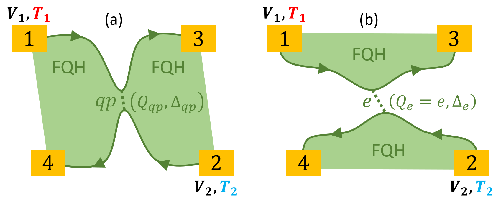
Figure 1: The standard setups for investigating quasiparticle [$qp$, panel (a)] and electron [$e$, panel (b)] tunneling in quantum Hall systems. Ohmic contacts 1 and 2 having voltages $V_{1}$ and $V_{2}$ respectively are used to inject electric current to the edges. Two FQH edges meet in the middle of the device, giving rise to the tunneling current $I_{T}$ and noise $S$, which are inferred from measurements at contacts 3 and 4. The dependence of $S$ and $I_{T}$ on $V_{1}-V_{2}$ enables a reliable extraction of the charge of the tunneling particle ($qp$ or $e$). Here we propose to extract the tunneling particle’s scaling dimension, $\Delta$, which governs the edge dynamics, using the temperatures $T_{1}$ and $T_{2}$ of the injected edge modes as additional experimental knobs. In the simple Abelian cases the exchange statistics of the tunneling particle is related to $\Delta$.

The so far most promising attempts to measure the scaling dimension concerned the dependence of the tunneling current at a QPC on the voltage bias between the two edges [36, 38]. The scheme should simultaneously extract both $Q$ and $\Delta$. Some experiments produce data that are congruent with the theoretically predicted curves [36, 38]. However, the extracted values of $Q$ and $\Delta$ vary greatly between different experimental configurations. Furthermore, in none of the configurations do both the fitted charge and the scaling dimension agree with those predicted by expected candidate theories [38]. Other experiments of the same type report that the tunneling current dependence on voltage significantly deviates from theoretically predicted curves [46, 14, 47, 48]. One possible explanation for such behavior is that changes in the bias voltage, $V=V_{1}-V_{2}$, cf. Fig. 1, affect the electrostatic balance at the QPC, changing its shape and the tunneling matrix element; the dependence of the tunneling amplitude on the voltage in turn alters the behavior of the tunneling current in a non-universal way.

This non-universality can be excluded by considering the ratio $F=S/(2eI_{T})$ (also called the Fano factor) of the excess noise $S$ appearing due to tunneling (the noise measured at contact 3 in the setups of Fig. 1 minus the Johnson-Nyquist noise $2\nu e^{2}k_{B}T_{1}/h$) to the tunneling current $I_{T}$. When the tunneling amplitude $\eta$ is small, both are $\propto\left|\eta\right|^{2}$, so that the ratio $F$ does not depend on $\eta$. In fact, this is the very trick that enables reliable determination of the quasiparticle charge in such setups [11, 12, 13, 14, 16, 17]. It has been theoretically shown that considering the dependence of $F$ on bias voltage at non-zero temperatures, in principle, allows for extracting not only charge but also the scaling dimension [49]. However, the term involving the scaling dimension turns out to be only a small correction to the main charge-dependent term and, therefore, cannot be reliably extracted from the standard experiments.

Considering temperature dependence instead of the voltage dependence is a new promising direction. On one hand, recent experiments developed a way of changing the edge temperature in a quick and electrically controllable manner [50, 51, 52, 53, 54, 55, 56]. On the other hand, a number of theoretical works considered the QPC physics when the two edges are at different temperatures [57, 58, 59, 60]. In particular, an intriguing effect of the excess noise dropping when the temperature imbalance between the edges is increased has been predicted [60].

In the present paper, we study the dependence of the Fano factor $F$ at the QPC on the temperatures of the two edges. We show that the scaling dimension can be extracted from the Fano factor’s temperature dependence. The paper is organized as follows. We briefly describe our key results in Sec. II. We then describe in Sec. III the model used to obtain these results for the noise in the setups of Fig. 1. In Sec. IV we analyze our predictions for some experimentally relevant scenarios. A discussion of the factors that may render the scaling dimension non-universal and of other experimental subtleties that may restrict the applicability of the proposed method is provided in Sec. V. We conclude with Sec. VI. For completeness, we provide a brief overview of the basics of the quantum Hall edge theory and of the meaning of the quasiparticles’ scaling dimensions in Appendix A. Technical details of the derivation of our results are relegated to Appendix B.

II Main Results

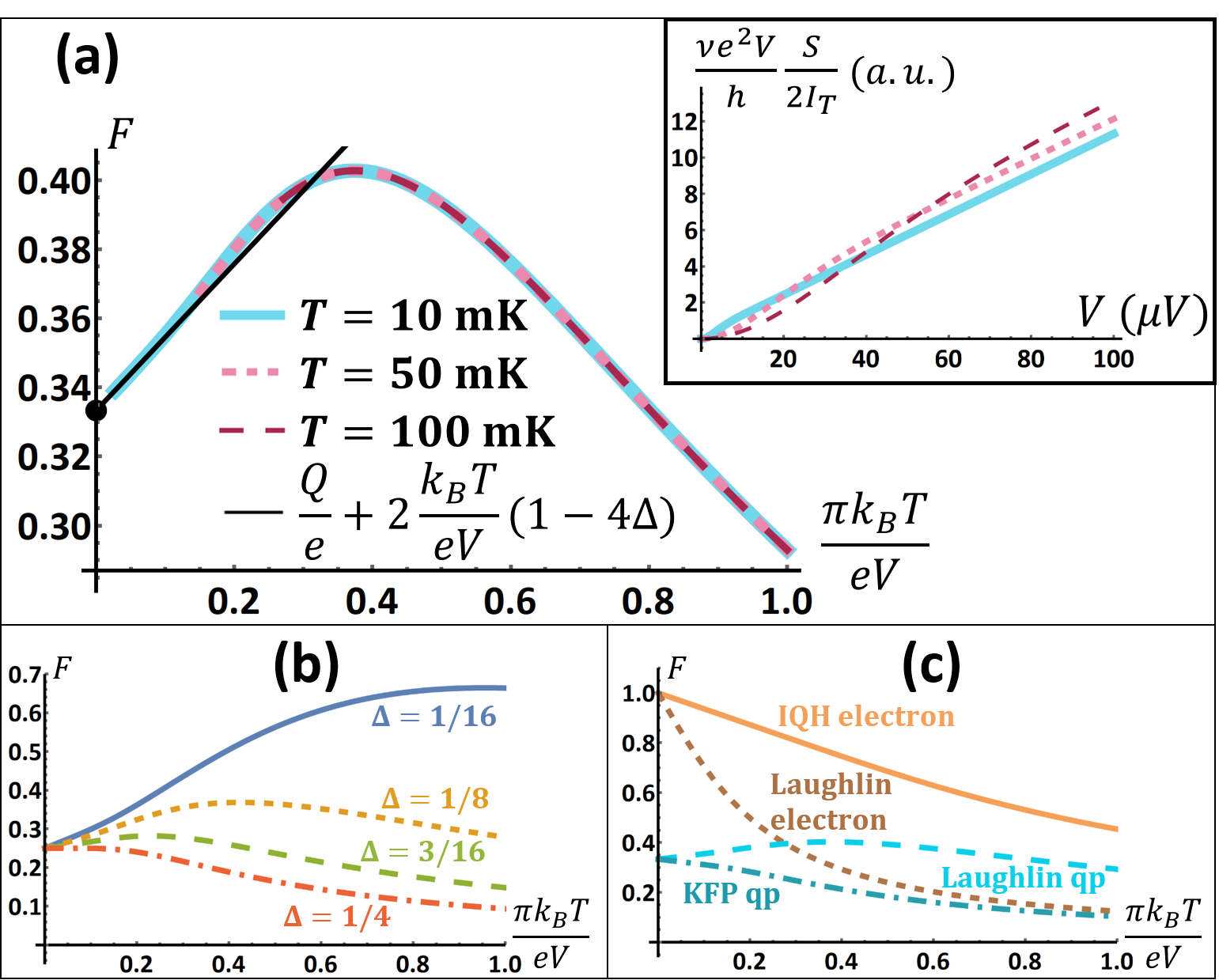
Figure 2: Fano factor’s dependence on temperature $T=T_{1}=T_{2}$ (cf. Fig. 1) as a tool for extracting the scaling dimensions of FQH quasiparticles and electrons. (a) The dependence of the Fano factor, $F=S/(2eI_{T})$ in Eq. (1), on $T/V$ for $\nu=1/3$ Laughlin quasiparticles $(Q=e/3,\Delta=1/6)$. The curve for each temperature corresponds to $V\in[0,100]\,\mathrm{\mu V}$. The curves collapse on top of each other, showing the universal behavior of the Fano factor. The thin black line corresponds to the asymptotic behavior in Eq. (2). The dot on the vertical axis corresponds to $F=Q/e$. Inset: The same data plotted in the way experiments are conventionally analyzed. The curves for different temperatures appear unrelated. (b) Fano factor vs. $T/V$ for quasiparticles that appear in various candidate theories of $\nu=5/2$ FQH effect: $Q=e/4$ (in all the theories), $\Delta=1/16$ ($K=8$ theory), $1/8$ (Pfaffian and PH-Pfaffian), $3/16$ (331 state) or $1/4$ (anti-Pfaffian) [61]. (c) Fano factor vs. $T/V$ for $\nu=1/3$ Laughlin quasiparticle $(Q=e/3,\Delta=1/6)$, one of the quasiparticles in the Kane-Fisher-Polchinski (KFP) $\nu=2/3$ fixed-point theory $(Q=e/3,\Delta=1/3)$, non-interacting integer quantum Hall (IQH) electrons $(Q=e,\Delta=1/2)$, electrons in the $\nu=1/3$ Laughlin state $(Q=e,\Delta=3/2)$ [5, 42, 43].

We first consider the case of equal temperatures of the two edges: $T_{1}=T_{2}=T$. In the inset of Fig. 2(a), we present the dependence of noise on the bias voltage for several temperatures $T$. Notice that we plot $\nu e^{2}V/h\times S/(2I_{T})=\nu e^{2}V/h\times eF$ so that the dependence of the tunneling amplitude on the bias voltage or the temperature cancels out. The slope at large $V$ corresponds to the charge of the tunneling quasiparticle. However, otherwise the curves do not appear to exhibit universality. In Appendix B.4.1 we show that in the regime of weak tunneling of quasiparticles or electrons across the QPC (cf. Fig. 1), the Fano factor is a universal function of $T/V$, namely

$$F=\frac{2Q}{\pi e}\mathrm{Im}\left[\psi\left(2\Delta+i\frac{QV}{2\pi k_{B}T}\right)\right],$$ (1)

where $Q$ and $\Delta$ are respectively the charge and the scaling dimension of the quasiparticle that tunnels, $k_{B}$ is the Boltzmann constant, the digamma function $\psi(x)=\Gamma^{\prime}(x)/\Gamma(x)$ is the logarithmic derivative of the gamma function, and $\mathrm{Im}$ stands for the imaginary part. This universality is illustrated in Fig. 2(a) where the curves of the inset of Fig. 2(a) are plotted as a function of $T/V$. Fitting experimental data to this curve should enable reliable extraction of the charge and the scaling dimension.

Further, consider the limit $eV\gg k_{B}T$, which corresponds to a typical regime investigated experimentally. Then

$$\left.F\right|_{eV\gg k_{B}T}=\frac{Q}{e}+2\frac{k_{B}T}{eV}(1-4\Delta)+O\left[\left(\frac{k_{B}T}{eV}\right)^{2}\right].$$ (2)

The first term of the expression represents the well-known result that the shot-noise Fano factor corresponds to the charge of the tunneling quasiparticle. The scaling dimension enters the second, subleading term. This subleading correction is a linear function of $T/V$ and can be quite sizeable, cf. Fig. 2(a).

In Fig. 2(b,c), we give several examples of the Fano factor behavior for quasiparticles corresponding to various quantum Hall states. Notice that quasiparticles of the same charge but different scaling dimensions produce notably different curves. In addition, we emphasize that the strongly-interacting nature of FQH states is manifest not only in the existence of fractional quasiparticles, but also in the electron scaling dimension, which can be inferred by the proposed method, cf. Figs. 2(c) and 1(b).

The origin of the above correction term can be roughly related to the quasiparticle exclusion statistics. Consider as an example non-interacting edges of $\nu=1$ integer quantum Hall states. At $T=0$, each edge is a Fermi sea of electrons occupied up to each edge’s Fermi level. Only the window of energies $eV$, where the electrons on one edge are not balanced by the electrons of the other edge is important. The electrons of different energies within this window tunnel independently, so the Pauli exclusion principle does not affect the observable quantities. At $T>0$, the edges of the Fermi seas become smeared. An electron within the $eV$ window can be hindered from tunneling to the other edge if this energy level is occupied (which happens with a $T$-dependent probability). This reduces the fluctuations of the occupation of this level, and thus reduces the noise and the Fano factor. This intuitive picture agrees with the prediction of Eq. (2) as for non-interacting electrons $\Delta=1/2$.

Had the electrons attracted each other or tended to bunch (as bosons do), the presence of an electron at an energy level before the QPC would increase the probability of tunneling of another electron from the opposite edge and would increase the noise. This is the case, e.g., when dealing with $\nu=1/3$ Laughlin quasiparticles (that can bunch up to $3$ in one quantum state and have $\Delta=1/6$). It is remarkable that quasiparticles with $\Delta=1/4$, (for example, semions) which for sufficiently simple edges are half-way between bosons and fermions in terms of the statistical phase $\theta=2\pi\Delta$, would produce no correction to the Fano factor in this regime.

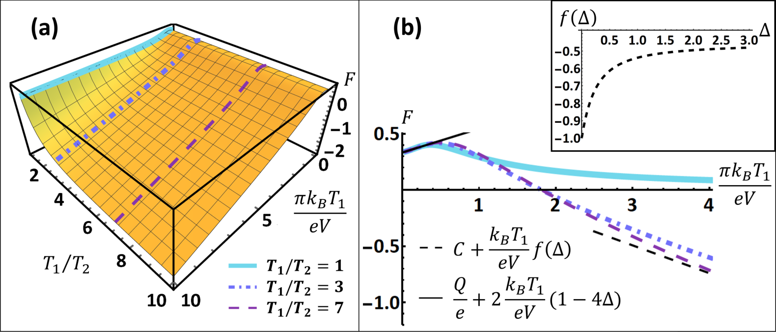
Figure 3: The Fano factor for the case of $T_{1}\geq T_{2}$ (cf. Fig. 1). (a) Plot of the universal function given in Eq. (3) illustrated for the Laughlin quasiparticle $(Q=e/3,\Delta=1/6)$. Lines denote the cuts corresponding to $T_{1}/T_{2}=1$, $3$, and $7$. (b) Cuts corresponding to $T_{1}/T_{2}=1$, $3$, and $7$ plotted as a function of $T_{1}/V$. At small $T_{1}/V$ the Fano factor’s behavior is described by Eq. (4) (solid black line). At large $T_{1}/V$, Eq. (5) gives the asymptotic behavior (dashed black line); the slope of the curves at $T_{1}/T_{2}=3$ and $7$ is quite close to the expected behavior, while the offset $C$ only converges to zero when $T_{1}/T_{2}\rightarrow\infty$. Inset—The slope $f(\Delta)$ entering Eq. (5) as a function of the quasiparticle scaling dimension.

It is important to emphasize two things. First, while the above consideration is qualitative and appeals to the intuition of non-interacting systems, we have derived Eqs. (1) and (2) using proper quantum Hall edge theory that takes the interacting nature of the FQH states into account. Second, the relation between the scaling dimension and quasiparticle statistics is not universal and holds only for sufficiently simple Abelian quantum Hall edges, when only modes of a single chirality are present on the edge. Therefore, it is correct to characterize the noise in terms of the scaling dimension $\Delta$, and not in terms of the quasiparticle statistics.

We next consider the situation of general temperatures, assuming without loss of generality $T_{1}\geq T_{2}$. In this case, the Fano factor can be expressed as a universal function of $T_{1}/V$ and $T_{1}/T_{2}$:

$$F=\mathcal{F}_{Q,\Delta}\left(\frac{\pi k_{B}T_{1}}{eV},\frac{T_{1}}{T_{2}}\right),$$ (3)

where the detailed expression is presented in Sec. III, Eq. (23). The universality is manifest in the function being determined only by the charge $Q$ and the scaling dimension $\Delta$ of the tunneling quasiparticle. All data for the Fano factor dependence on the bias voltage $V$ and the two temperatures, $T_{1}$ and $T_{2}$, should collapse on a two-dimensional (2D) surface, which is determined only by the values of $Q$ and $\Delta$. We illustrate the behavior of this function for Laughlin quasiparticles in Fig. 3(a).

The expression in Eq. (3) simplifies in some limiting cases. First, we show in Appendix B.4.1 that for $T_{1}=T_{2}=T$, Eq. (3) reduces to Eq. (1). Second, we show in Appendix B.4.3 that in the regime $eV\gg k_{B}T_{1}\geq k_{B}T_{2}$, Eq. (3) simplifies to

$$\left.F\right|_{eV\gg k_{B}T_{1,2}}=\frac{Q}{e}+2\frac{k_{B}T_{1}}{eV}(1-4\Delta)+O\left[\left(\frac{k_{B}T_{1,2}}{eV}\right)^{2}\right].$$ (4)

Third, we show in Appendix B.4.2 that in the regime dominated by the temperature imbalance, $k_{B}T_{1}\gg eV,\,k_{B}T_{2}$,

$$\left.F\right|_{k_{B}T_{1}\gg eV,\,k_{B}T_{2}}=\frac{k_{B}T_{1}}{eV}f(\Delta)+O\left[\frac{eV}{k_{B}T_{1}},\frac{k_{B}T_{1}}{eV}\left(\frac{T_{2}}{T_{1}}\right)^{2}\right],$$ (5)

where $f(\Delta)$ is a function of the scaling dimension, whose behavior is presented in the inset of Fig. 3(b). Notice that the bias voltage enters the expression of Eq. (5), but the quasiparticle charge $Q$ does not. We illustrate the asymptotic behaviors of Eqs. (4, 5) in Fig. 3(b).

Note that the Fano factor can become negative when $T_{1}\neq T_{2}$, cf. Fig. 3. This is due to the excess noise becoming negative in the presence of temperature imbalance between the edges, similarly to the effect predicted recently in Ref. [60]. We emphasize the non-triviality of this result: while raising the temperature of one edge is expected to affect the intensity of the tunneling processes, the Fano factor’s behavior shows that the noise and the current are affected in different ways. The total noise at contact $3$ (cf. Fig. 1) comprises the excess noise $S$, as well as the Johnson–Nyquist noise of the FQH edge (which is typically subtracted in experiments). The latter, of course, grows as $T_{1}$ is increased, as does the total noise at contact $3$. However, the excess noise $S$ involving the contribution of the tunneling processes becomes negative. Knowing the extent of its negativity enables one to extract the quasiparticle’s scaling dimension $\Delta$, cf. Eq. (5) and Fig. 3(b, inset).

The negative excess noise (and thus the negative Fano factor) can be understood from comparing the noise at contact 3 in the presence and in the absence of the tunneling contact. In the absence of tunneling at the QPC, the noise measured at contact 3 is the Johnson–Nyquist noise corresponding to $T_{1}$. In the presence of tunneling, part of the Johnson–Nyquist noise from the upper edge leaks to the lower edge. Similarly, the noise from the lower edge leaks to the upper edge. The shot noise generated by tunneling can be, to a good approximation, ignored since the temperature imbalance dominates the system. As the upper edge has a higher temperature, overall the noise at contact 3 is reduced. The extent of this reduction is controlled by the intensity of the tunneling processes, i.e., by the scaling dimension $\Delta$. The lower the scaling dimension, the more intense the tunneling is, which correlates with the behavior of $f(\Delta)$ in the inset of Fig. 3(b).

We warn the reader against hastily interpreting the above behaviors in terms of particle statistics or identifying a specific behavior with that of classical particles. As is discussed above and in Appendix A, the scaling dimension is not always simply related to the quasiparticle statistics. Further, even in the cases when this relation is valid, predictions based on naive models of particles with corresponding statistics can be misleading. For example, the results of Ref. [64] show that the predictions for the noise in the presence of small temperature imbalance are different for the model of free bosons and the model of chiral Luttinger liquid with integer scaling dimensions (that translate into the bosonic statistics of quasiparticles through $\theta=2\pi\Delta$). Therefore, the system’s dynamics cannot be described in terms of non-interacting quasiparticles of the respective statistics.

Overall, we argue that the Fano factor is a powerful instrument for extracting not only the charge but also the scaling dimension of FQH quasiparticles. In particular, if investigated as a function of the edge temperatures.

III General results for thermal noise at a QPC

We now proceed to describe our theoretical approach and the obtained results. Our calculations are valid for any FQH edge theory for which the FQH edges on either side of the QPC can be assigned a well-defined voltage and temperature. For simplicity, however, we focus in this section on the Abelian theories. The generalization to non-Abelian theories is straightforward and is discussed in Appendix A.

The action of the general Abelian FQH edge is given in terms of $N$ bosonic fields, $\phi_{l},\;i=1,\dots,N$

$$S=\frac{1}{4\pi}\int dxdt\sum_{l}\left(-\chi_{l}\partial_{x}\phi_{l}\partial_{t}\phi_{l}-v_{l}\left(\partial_{x}\phi_{l}\right)^{2}\right),$$ (6)

where $\chi_{l}=\pm 1$ and $v_{l}>0$ are the chirality and velocity of the $l$th mode, respectively. These fields satisfy the commutation relations

$$\left[\phi_{l}(x,t),\phi_{l^{\prime}}(x^{\prime},t^{\prime})\right]=i\pi\chi_{l}\text{sgn}\left(\xi_{l}-\xi_{l}^{\prime}\right)\delta_{l,l^{\prime}},$$ (7)

where $\xi_{l}\equiv x-\chi_{l}v_{l}t$. Density and current operators along the edge are given by

$$\rho=\frac{1}{2\pi}\sum_{l}q_{l}\partial_{x}\phi_{l};\;j=-\frac{1}{2\pi}\sum_{l}q_{l}\partial_{t}\phi_{l},$$ (8)

where, as explained in Appendix A, $q_{l}$ are numbers that define the charge-carrying properties of the edge modes. They are constrained via the relationship

$$\sum_{l}\chi_{l}q_{l}^{2}=\nu,$$

where $\nu$ is the filling factor.

The edge supports quasiparticles of the form

$$\psi_{a}(x,t)\propto e^{i\bm{a}\cdot\bm{\phi}(x,t)},$$ (9)

where $\bm{\phi}(x,t)\equiv(\phi_{1}(x,t),\dots,\phi_{N}(x,t))$ and $\bm{a}=(a_{1},\dots,a_{N})$ are vectors composed of the bosonic fields and real numbers, respectively. The vector $\bm{a}$, while being real-valued, can only take a discrete set of values reflecting the set of possible quasiparticles. Such quasiparticles are characterized by two important quantum numbers: the electric charge

$$Q_{a}=e\sum_{l}\chi_{l}q_{l}a_{l}$$ (10)

and the scaling dimension

$$\Delta=\frac{1}{2}\sum_{l}a_{l}^{2}.$$ (11)

The set of allowed quasiparticles must include electrons with $Q=e$.

We model the QPC by a term in the Hamiltonian which describes tunneling of quasiparticles between the edges,

$$H_{T} =\sum_{a}\eta_{a}\psi_{a}^{(u)\dagger}\psi_{a}^{(d)}+\text{h.c.}$$

$$\equiv\sum_{a}\left[\eta_{a}A_{a}+\eta_{a}^{*}A_{a}^{\dagger}\right];\;A_{a}\equiv\psi_{a}^{(u)\dagger}\psi_{a}^{(d)},$$

with superscripts $u/d$ denoting the upper/lower edge, respectively. The current operator at the upper/lower drain (labeled 3 and 4 in Fig. 1) will be given by

$$\hat{I}_{3/4}=j^{(u/d)}\mp\hat{I}_{T}$$ (12)

where $j^{(u/d)}$ is the current operator of the unperturbed edge at the QPC location, cf. Eq. (8), and $I_{T}$ is the tunneling current (i.e., the current that leaves the upper edge and enters the lower edge). In the operator form, this is given by

$$\hat{I}_{T}=i\sum_{a}Q_{a}\left[\eta_{a}A_{a}-\eta_{a}^{*}A_{a}^{\dagger}\right].$$ (13)

We wish to calculate the average tunneling current, $I_{T}\equiv\langle\hat{I}_{T}\rangle$, the auto-correlations at each of the drains, and the cross-correlations between them. We define the DC noise correlations between drains $i,j$ as

$$S_{i,j}(\omega=0)=\int dt\langle\Delta\hat{I}_{i}(0)\Delta\hat{I}_{j}(t)+\Delta\hat{I}_{j}(t)\Delta\hat{I}_{i}(0)\rangle,$$ (14)

where $\Delta\hat{I}_{i}\equiv\hat{I}_{i}-\langle\hat{I}_{i}\rangle$. The auto-correlations and cross-correlations are not independent, but satisfy the relation $S_{3,3}+S_{4,4}+2S_{3,4}=2\nu\frac{e^{2}}{h}k_{B}\left(T_{1}+T_{2}\right)$ that links their sum to the Johnson-Nyquist noise, cf. Appendix B.2. It is, therefore, sufficient to investigate only the auto-correlations $S_{3,3}$ and $S_{4,4}$.

Without loss of generality, we focus in what follows on the excess noise measured at drain $3$, $S\equiv S_{3,3}-2\frac{e^{2}}{h}\nu k_{B}T_{1}$. Defining $\lambda\equiv T_{1}/T_{2}$, we find

$$S= S_{TT}+2S_{0T}$$ (15)

$$S_{TT}= 4\sum_{a}Q_{a}^{2}G_{a}\mathcal{I}_{1}\left(\frac{Q_{a}V}{\pi k_{B}T_{1}},\frac{1}{\lambda},{2\Delta_{a}}\right),$$ (16)

$$S_{0T}= -\frac{4i}{\pi}\sum_{a}Q_{a}^{2}G_{a}\mathcal{I}_{2}\left(\frac{Q_{a}V}{\pi k_{B}T_{1}},\frac{1}{\lambda},{2\Delta_{a}}\right)$$ (17)

$$-2\sum_{a}Q_{a}^{2}G_{a}\mathcal{I}_{1}\left(\frac{Q_{a}V}{\pi k_{B}T_{1}},\frac{1}{\lambda},{2\Delta_{a}}\right),$$

$$I_{T}= 2i\sum_{a}Q_{a}G_{a}\mathcal{I}_{3}\left(\frac{Q_{a}V}{\pi k_{B}T_{1}},\frac{1}{\lambda},{2\Delta_{a}}\right),$$ (18)

where we have defined the integrals

$$\mathcal{I}_{1}\left(a,b,c\right)\equiv\int\limits_{-\infty}^{\infty}dy\frac{\cos{\left(a\left(y-\frac{i\pi}{2}\right)\right)}}{\left[\cosh\left(y\right)i\sinh\left(b\left(y-\frac{i\pi}{2}\right)\right)\right]^{c}},$$ (19)

$$\mathcal{I}_{2}\left(a,b,c\right)\equiv\int\limits_{-\infty}^{\infty}dy\frac{y\cos{\left(a\left(y-\frac{i\pi}{2}\right)\right)}}{\left[\cosh\left(y\right)i\sinh\left(b\left(y-\frac{i\pi}{2}\right)\right)\right]^{c}},$$ (20)

$$\mathcal{I}_{3}\left(a,b,c\right)\equiv\int\limits_{-\infty}^{\infty}dy\frac{\sin{\left(a\left(y-\frac{i\pi}{2}\right)\right)}}{\left[\cosh\left(y\right)i\sinh\left(b\left(y-\frac{i\pi}{2}\right)\right)\right]^{c}},$$ (21)

and

$$G_{a}\equiv\left|\eta_{a}\right|^{2}\left(\pi k_{B}T_{2}\right)^{4\Delta_{a}-1}\lambda^{2\Delta_{a}-1}\prod_{l}v_{l}^{-2a_{l}^{2}}$$ (22)

is the effective tunneling constant for each quasiparticle. The derivation of these expressions is given in Appendix B.2.

The term $S_{TT}$ arises from self-correlations of the tunneling current, while $S_{0T}$ represents cross-correlations between the current $j^{(u/d)}$ flowing along the unperturbed edge and the tunneling current. The physical mechanism giving rise to these cross-correlations and its rough relation to the exclusion statistics were described in Sec. II.

Typically, a single quasiparticle possessing the smallest scaling dimension $\Delta_{a}=\Delta$ is assumed to dominate the tunneling processes at the QPC. Denoting its charge $Q_{a}$ as $Q$, we find the Fano factor

$$F\equiv\frac{S}{2eI_{T}}=-\frac{2Q}{\pi e}\frac{\mathcal{I}_{2}\left(\frac{QV}{\pi k_{B}T_{1}},\frac{T_{2}}{T_{1}},{2\Delta}\right)}{\mathcal{I}_{3}\left(\frac{QV}{\pi k_{B}T_{1}},\frac{T_{2}}{T_{1}},{2\Delta}\right)}.$$ (23)

Note that $F$ does not feature the non-universal tunneling amplitude $\left|\eta_{a}\right|^{2}$.

IV Experimentally relevant scenarios

In this section we explore several parameters’ regimes, demonstrating how the expression for the Fano factor in Eq. (23) enables discrimination between different values of $\Delta$. These regimes correspond to different cuts of the 2D surface presented in Fig. 3 and illustrate how the three experimental knobs ($V$, $T_{1}$, and $T_{2}$) affect the Fano factor. We choose the parameters of these regimes to be compatible with modern experiments [17, 18, 19, 20, 68].

IV.1 Equal temperatures

The case of equal temperatures was discussed at length in Sec. II. For $T_{1}=T_{2}\equiv T$, Eq. (23) simplifies to Eq. (1), there the Fano factor is equal to the imaginary part of the digamma function whose argument depends solely on the parameters $Q$ and $\Delta$, and the ratio $eV/k_{B}T$. At the high-voltage limit, $eV\gg k_{B}T$, the expression further simplifies to a linear function of $k_{B}T/eV$, see Eq. (2).

As shown in Fig. 2, this universal function enables easy extraction of the quantum numbers of interest by plotting the Fano factor as a function of the ratio $k_{B}T/eV$. The quasiparticle charge will be given by the intersection of the plot with the $y$ axis, and the scaling dimension by the slope of the curve at low $k_{B}T/eV$.

IV.2 Different temperatures (small V)

In this regime, the bias voltage $V$ is kept constant and small compared with both edge temperatures $T_{1}$ and $T_{2}$. One of these temperatures is then swept over a substantial range, which in an experimental setup will be restricted from above by the bulk gap. The behavior of the Fano factor in this regime is demonstrated in Fig. 4(a) for candidate theories of the potentially non-Abelian $\nu=5/2$, and in Fig. 4(b) for characteristic quasiparticles at $\nu=1/3$, $2/3$, and $1$.

The Fano factor when $T_{1}=T_{2}$ can be obtained from Eq. (1); note that at $V=0$, this will be zero. As $T_{1}$ is increased (decreased), the Fano factor decreases (increases), becoming strongly negative (positive). This is consistent with the results of Ref. [60], in which a temperature imbalance leads to noise reduction on the hot edge, and a noise increase on the cold edge. This regime exhibits a particularly instructive asymptote where the dominant energy scale of the system is the temperature of the hot edge, i.e., $\lambda=T_{1}/T_{2}\gg 1$. In this limit, the Fano factor becomes a linear function of the ratio $k_{B}T_{1}/eV$, cf. Eq. (5). The scaling dimension alone determines the slope via a negative, monotonously increasing function $f(\Delta)$, cf. the inset of  Fig. 3(b). The cold edge temperature $T_{2}$ drops out entirely from the description. Note the values of $\left|F\right|\gg 1$, which appear due to $k_{B}T_{1}\gg eV$.

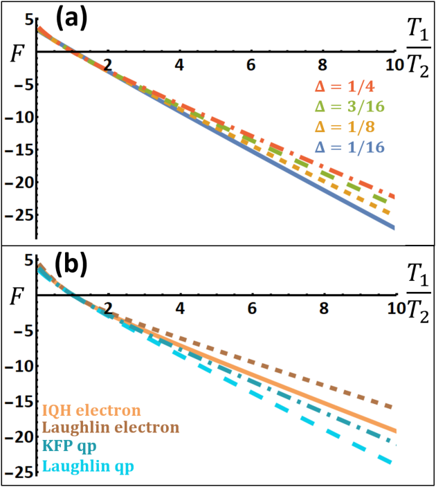
Figure 4: The Fano factor vs. temperature ratio $T_{1}/T_{2}$ for small voltage ($eV=0.1\pi k_{B}T_{2}$). Remark the large $\Delta$-dependent negative values of the Fano factor and its very weak dependence on the charge $Q$, cf. Eq. (5). (a) Quasiparticles that appear in various candidate theories of $\nu=5/2$ FQH effect: $Q=e/4$ (in all the theories), $\Delta=1/16$ ($K=8$ theory), $1/8$ (Pfaffian and PH-Pfaffian), $3/16$ (331 state) or $1/4$ (anti-Pfaffian) [61]. (b) $\nu=1/3$ Laughlin quasiparticle $(Q=e/3,\Delta=1/6)$, one of the quasiparticles in the Kane-Fisher-Polchinski (KFP) $\nu=2/3$ fixed-point theory $(Q=e/3,\Delta=1/3)$, non-interacting integer quantum Hall (IQH) electrons $(Q=e,\Delta=1/2)$, electrons in the $\nu=1/3$ Laughlin state $(Q=e,\Delta=3/2)$ [5, 42, 43].

For physical intuition, we once again appeal to the more familiar case of Fermi-Dirac distributions. When $k_{B}T_{1}\gg k_{B}T_{2},eV$, the Fermi sea at the hot edge is so dramatically smeared that any deformations of the cold edge are comparatively negligible. As such, the noise will depend solely on $T_{1}$. The tunneling current, meanwhile, is in the Ohmic limit $I_{T}\propto T_{1}^{4\Delta-2}V$, which leads to $F\propto V^{-1}$. We note that had we been interested in the noise measured at contact 4 (cf. Fig. 1), belonging to the colder edge, the respective Fano factor would retain a term proportional to $T_{2}/T_{1}$.

The monotonicity of the function $f(\Delta)$ makes this regime useful to differentiate between similar theories with different scaling dimensions. However, the non-linear form of $f(\Delta)$ means that in this regime $F$ is highly sensitive for $\Delta<1/2$, less sensitive for $1/2<\Delta<3/2$, and can hardly discriminate different $\Delta>3/2$.

IV.3 Different temperatures (large voltage)

Another useful regime exists when $eV\gg k_{B}T_{2}$, while $k_{B}T_{1}$ takes any value between them. We present the data for candidate theories at $\nu=5/2$ and for characteristic quasiparticles at $\nu=1/3$, $2/3$, and $1$ in Fig. 5, panels (a) and (b) respectively.

As long as $k_{B}T_{1}\ll eV$, the Fano factor obeys Eq. (4), in particular giving the charge $Q$ at the limit $T_{1}\rightarrow 0$. The dependence on $\Delta$ in this regime is linear, which guarantees the same sensitivity over the whole range of $\Delta$.

For $k_{B}T_{1}\lesssim eV$, the analytical understanding of the behavior is lacking. However, Fig. 5 shows that this regime has its own distinctive features. Note that $F$ can become negative. We find that it always becomes negative at $k_{B}T_{1}\simeq eV$, with the exact location of the crossover point determined by the scaling dimension. This agrees with the intuition of the $k_{B}T_{1}\gg eV$ regime, cf. Sec. IV.2.

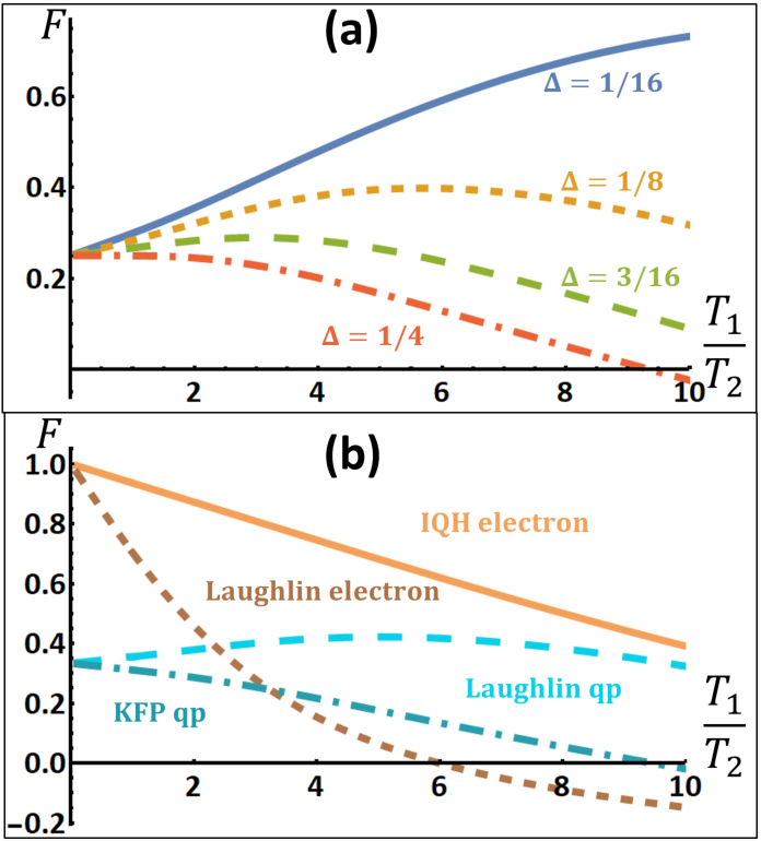
Figure 5: The Fano factor vs. temperature ratio $T_{1}/T_{2}$ for a large voltage ($eV=10\pi k_{B}T_{2}$). Measuring this dependence, cf. Eq. (23), one can extract both the charge $Q$ (which is obtained at $T_{1}/T_{2}\rightarrow 0$) and the scaling dimension $\Delta$ of the tunneling particle (which dictates the form of the curve). (a) Quasiparticles that appear in various candidate theories of $\nu=5/2$ FQH effect: $Q=e/4$ (in all the theories), $\Delta=1/16$ ($K=8$ theory), $1/8$ (Pfaffian and PH-Pfaffian), $3/16$ (331 state) or $1/4$ (anti-Pfaffian) [61]. (b) $\nu=1/3$ Laughlin quasiparticles $(Q=e/3,\Delta=1/6)$, one of the quasiparticles in the Kane-Fisher-Polchinski (KFP) $\nu=2/3$ fixed-point theory $(Q=e/3,\Delta=1/3)$, non-interacting integer quantum Hall (IQH) electrons $(Q=e,\Delta=1/2)$, electrons in the $\nu=1/3$ Laughlin state $(Q=e,\Delta=3/2)$ [5, 42, 43].

V Discussion

In the above sections, we have described a method for determining the scaling dimension of quantum Hall quasiparticles and analyzed some experimentally relevant regimes. At the same time, it is important to understand what information is encoded in the scaling dimension. It is also important to be aware of the experimental subtleties that may affect the applicability of the above considerations. We discuss these issues below.

In the fully chiral edges (both Abelian and non-Abelian), the scaling dimension is universal as it is related to the quasiparticle statistics, cf. Appendix A. Non-chiral edges do not feature this robustness: interactions between counterpropagating edge modes can lead to a change in the scaling dimension [42, 43, 44, 45]. Further, edge reconstruction can add counterpropagating modes to chiral edges [69, 44] and thus facilitate a change in the scaling dimension. Yet even under these circumstances the scaling dimension remains an important quantity to measure. First, the scaling dimension reflects the properties of the edge including the reconstructions and intermode interactions. Second, the scaling dimension of the quasiparticle that dominates tunneling is typically larger in the reconstructed theory. Therefore, measuring a specific scaling dimension excludes underlying non-reconstructed theories, where the scaling dimension is bigger than the one measured.

Another mechanism undermining the universality of the scaling dimension is the electrostatic (screened Coulomb) interactions in the vicinity of the QPC [70, 61]. These may renormalize the scaling dimension in the vicinity of the QPC, so that it does not reflect the properties of the quasiparticles away from the QPC. One can minimize these interaction effects by designing the device such that counter propagating modes are close to each other only at short length $l_{{\rm int}}$ near the QPC. At low energies such that $v/E\gg l_{{\rm int}}$ ($v$ is the characteristic edge velocity) the Coulomb interaction will not affect the scaling dimension. The results of Ref. [21] suggest that it is indeed possible to have experiments, where the electrostatic interactions in the vicinity of the QPC do not play a major role.

The above non-universalities may affect the interpretation of the extracted scaling dimension. However, they do not affect the validity of our method. Below, we discuss subtleties that may be present in realistic experimental setups and may require modifications to the proposed method.

The considerations of this paper assume that each edge is at equilibrium. However, edges featuring counterpropagating modes may not be at equilibrium [71, 72, 73, 74, 75, 76, 77]. Some types of non-equilibrium may be tolerated. For example, the $\nu=2/3$ edge can have temperature gradients along the edge while locally all the modes have the same temperature [71, 73, 74]. This type of non-equilibrium can be taken into account simply: the physics at the QPC is described by the local temperature. As long as the temperature at the QPC can be estimated independently, the scaling dimension can be extracted.

On the other hand, if counterpropagating modes interact very weakly, they can be out of equilibrium even locally, invalidating the assumptions of the present work. Such non-equilibrium will, however, lead to a non-quantized Hall conductance for charged counterpropagating modes [42, 43]. The equilibration properties of counterpropagating neutral modes can be investigated by measuring the excess noise of a single edge (with no tunneling at a QPC) [71, 73, 74, 78, 55, 56, [Seealso]Spanslatt2020].

Finally, one could expect complications due to interfaces between the Ohmic contacts and the quantum Hall edges. Indeed, the transport properties (e.g., conductance) of the Luttinger liquid depend crucially on the nature of its interface with external leads (see, e.g., Refs. [80, 81]). Quantum Hall edges may also experience such non-universal effects [82, 83, 84], implying the need to employ other methods for probing the noise generated at a QPC, e.g., that of Ref. [85]. However, we expect this to be unnecessary. Such non-universalities should have no influence on the observations as long as the charge transport along the edge channels is fully chiral (i.e., for the edges where all modes have the same chirality, as well as for generic edges with modes of different chiralities in the regime of strong equilibration [71]). All the current and noise generated at the QPC must then reach the respective Ohmic contact, as they cannot be reflected back at the interface.

VI Conclusions

In this paper we have proposed a method for determining the scaling dimension of quantum Hall quasiparticles based on the measurements of the noise generated at a QPC. The method relies on analyzing the dependence of the Fano factor on the bias voltage and the temperatures of the quantum Hall edges. We expect the extraction of the scaling dimension via the proposed method to be as robust as the extraction of the quasiparticle charge from the Fano factor.

While our method is expected to enable reliable extraction of the scaling dimension and excludes some non-universal effects, it is important to realize that the scaling dimension itself may not be universal. Yet even when the scaling dimension is non-universal, it remains an important quantity that characterizes the dynamics of the system. For fully chiral edges (both Abelian and non-Abelian), the scaling dimension is universal, as it is related to the quasiparticle statistics.

Appendix A Background on quantum Hall edge theory

In this section we remind the reader some well-known theoretical results which apply to all existing quantum Hall edge models (integer and fractional, Abelian and non-Abelian, fully chiral or featuring counterpropagating modes). We only focus here on the aspects relevant for the present work, in particular, the role of the scaling dimension in describing the edge properties. For a more comprehensive summary of the theory in the notation that is close to the notation used in the present paper, see Ref. [86, Sec. III] or Ref. [58, Sec. IV]. Among other details, these references explain the relation between the standard $K$-matrix-based notation for Abelian theories [8] and the present notation.

A.1 The structure of a general edge model

The behavior of quantum Hall edges is theoretically described by the chiral Luttinger liquid theory and its non-Abelian generalizations [5, 6, 8, 87]. A quantum Hall edge may consist of an arbitrary number $N$ of edge modes. Each mode has a direction of propagation (chirality) that we denote $\chi_{l}=\pm 1$, $l=1,...,N$, cf. Fig. 6. Some modes contribute to the electric transport by carrying charged excitations, while others may carry only neutral excitations. The size of a mode’s contribution to the electric transport can be encoded in numbers $q_{l}\geq 0$. When a mode does not carry charged excitations, $q_{l}=0$. If the edge mode is at equilibrium and its electrostatic potential is $V$, it carries current $I_{l}=\frac{e^{2}}{h}q_{l}^{2}\chi_{l}V$. The sign of $I_{l}$ reflects the current direction, i.e., the mode’s chirality. Fixing the Hall conductance to $\nu e^{2}/h$, therefore, requires $\sum_{l}q_{l}^{2}\chi_{l}=\nu$. Each mode has a velocity $v_{l}>0$ with which its excitations propagate.

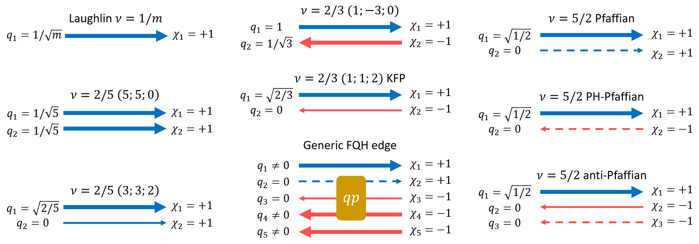
Figure 6: Examples of various quantum Hall edge structures. Note that the same filling factor $\nu$ may admit multiple edge structures. Each edge structure is characterized by a number of gapless modes. Each mode is chiral (rightmoving, $\chi=+1$ [blue arrows], or leftmoving, $\chi=-1$ [red arrows]). Modes can be charged (thick lines) and neutral (thin). Further, they can be Abelian (solid) or support non-Abelian excitations (dashed). Quasiparticles (qp) that can tunnel between edges of one FQH sample generically combine degrees of freedom from several modes.

The bulk and the edge of a quantum Hall sample can host local quasiparticles. At the edge, for each quasiparticle one can define the second-quantized quasiparticle operator $\psi_{\mathrm{qp}}(x,t)$, where $x$ is the position along the edge and $t$ is the time. The quasiparticle might be associated with one mode only. However, in general, a quasiparticle is distributed over several modes: $\psi_{\mathrm{qp}}(x,t)=\prod_{l}O_{l}(x,t)$, where $O_{l}$ is an operator belonging to mode $l$. The distribution can be quantified by a set of numbers $h_{l}\geq 0$, reflecting the scaling properties of operators $O_{l}$. For the modes contributing to the electric transport, one defines $a_{l}=\sqrt{h_{l}}$. The electric charge of the quasiparticle can then be expressed as

$$Q=e\bm{q}\circ\bm{a}=e\sum_{l}q_{l}\chi_{l}a_{l},$$ (24)

where $e$ is the electron charge. It is also convenient to define the scaling dimension

$$\Delta=\frac{1}{2}\sum_{l}h_{l}$$ (25)

and the conformal spin

$$s=\frac{1}{2}\sum_{l}\chi_{l}h_{l}.$$ (26)

When the edge is at equilibrium, characterized by electrostatic potential $V$ and temperature $T$, one can write the self-correlation function of a quasiparticle on the edge as

$$\langle\mathcal{T}\psi_{\mathrm{qp}}^{\dagger}(x,t)\psi_{\mathrm{qp}}(0,0)\rangle\\ =\prod_{l}\left[\left(\frac{\pi k_{B}T}{i\hbar v_{l}\sinh\pi k_{B}Tt_{l}/\hbar}\right)^{h_{l}}\exp\left(\frac{i}{\hbar}eq_{l}\chi_{l}a_{l}Vt_{l}\right)\right],$$ (27)

and

$$\langle\mathcal{T}\psi_{\mathrm{qp}}(x,t)\psi_{\mathrm{qp}}^{\dagger}(0,0)\rangle\\ =\prod_{l}\left[\left(\frac{\pi k_{B}T}{i\hbar v_{l}\sinh\pi k_{B}Tt_{l}/\hbar}\right)^{h_{l}}\exp\left(-\frac{i}{\hbar}eq_{l}\chi_{l}a_{l}Vt_{l}\right)\right],$$ (28)

where $t_{l}=t-\chi_{l}x/v_{l}-i0^{+}\mathrm{sgn}\,t$ with $0^{+}$ being the infinitesimally small positive number and $\mathcal{T}$ stands for the time ordering of the operators.

Note how the above correlation functions reflect the quasiparticle distribution over several edge modes. The correlation function in Eq. (28) represents the quantum amplitude of putting a quasiparticle on the edge at $t=0$ and extracting it from a different location at a later time $t>0$. The size of this amplitude decays exponentially for $T\neq 0$ (power-law when $T\rightarrow 0$) with the distance from the expected quasiparticle location on each edge mode: $x_{\mathrm{expected}}^{(j)}=\chi_{l}v_{l}t$. However, the expected location $x_{\mathrm{expected}}^{(l)}$ is different for different modes $l$. This reflects that once the quasiparticle is put onto the FQH edge, different parts of it propagate independently. This is reminiscent of spin-charge separation in Luttinger liquids: once an electron is injected into a Luttinger liquid, its spin and charge propagate with different velocities [90].

This concludes the minimalistic introduction into the structure of a general quantum Hall edge model. Next, in Sec. A.2, we focus on discussing the main properties of the quasiparticles, namely, the charge $Q$, the conformal spin $s$, the scaling dimension $\Delta$, and their connection to the quasiparticle statistics and to the setup of Fig. 1.

A.2 Properties of the FQH quasiparticles and their connection to the setup in Fig. 1

In order to explain the meaning of the quasiparticle scaling dimension $\Delta$ in Eq. (25) and conformal spin $s$ in Eq. (26), as well as their connection to the statistics, we will analyze the quasiparticle correlation functions in Eqs. (27–28). Consider first the same-position correlation function:

$$\langle\psi_{\mathrm{qp}}(0,t>0)\psi_{\mathrm{qp}}^{\dagger}(0,0)\rangle\propto\frac{e^{-iQVt/\hbar}}{\left(\sinh\pi k_{B}Tt/\hbar\right)^{2\Delta}}.$$ (29)

The oscillating exponential confirms the meaning of the quasiparticle charge $Q$ defined in Eq. (24): creating a quasiparticle adds energy $QV$ to the edge. The scaling dimension $\Delta$ controls the decay of self-correlations with time.

Consider now the correlation of quasiparticles at the same time but different positions. These can be obtained from Eqs. (27–28) by taking the limit $t\rightarrow 0$ while keeping $t>0$ and using the translational invariance of the correlation functions:

$$\langle\psi_{\mathrm{qp}}^{\dagger}(x,0)\psi_{\mathrm{qp}}(0,0)\rangle\\ \propto\prod_{l}\left[-i\sinh\frac{\pi k_{B}T\left(i0^{+}+\chi_{l}x/v_{l}\right)}{\hbar}\right]^{-h_{l}},$$ (30)

$$\langle\psi_{\mathrm{qp}}(0,0)\psi_{\mathrm{qp}}^{\dagger}(x,0)\rangle\\ \propto\prod_{l}\left[-i\sinh\frac{\pi k_{B}T\left(i0^{+}-\chi_{l}x/v_{l}\right)}{\hbar}\right]^{-h_{l}}.$$ (31)

Ignoring the infinitesimal imaginary part, one sees that the two expressions are connected by a factor $\prod_{l}(-1)^{-h_{l}}$. The infinitesimal imaginary part prescribes what root of unity one should take in each factor depending on the chirality $\chi_{l}$, so that

$$\langle\psi_{\mathrm{qp}}(0,0)\psi_{\mathrm{qp}}^{\dagger}(x,0)\rangle=e^{-2i\pi s\,\mathrm{sgn}\,x}\langle\psi_{\mathrm{qp}}^{\dagger}(x,0)\psi_{\mathrm{qp}}(0,0)\rangle.$$ (32)

This suggests that exchanging two quasiparticles produces the statistical factor $e^{i\theta}$ with $\theta=\pm 2\pi s$. Therefore, the conformal spin in Eq. (26) reflects the statistics of the quasiparticles. The last statement is accurate only for Abelian quasiparticles. If the quasiparticles possess non-Abelian statistics, this requires at least four quasiparticles to be manifest and cannot be seen via two-point correlation functions. Therefore, the conformal spin $s$ only captures the Abelian part of the statistics.

When the edge contains modes of one chirality only (all $\chi_{l}=\chi$), then $s=\chi\Delta$, as can be seen from Eqs. (25–26). In this sense, measuring the scaling dimension allows one to infer the quasiparticle statistics. We emphasize once more that this statement is only exactly valid for edges that are fully chiral and feature no non-Abelian quasiparticles. However, even when the correspondence between the statistics and the scaling dimension does not hold, the scaling dimensions of different quasiparticles in the theory are an important property of the edge theory and are valuable to measure.

Tunneling experiments as in Fig. 1 enable access to the scaling dimension. Since the tunneling happens only at one point on each edge, such experiments can be described in terms of the same-position correlation functions such as in Eq. (29). In fact, when the tunneling is weak, only two-point correlation functions, containing one creation and one annihilation operator for a quasiparticle, appear in the calculation, cf. Appendix B. Therefore, nothing but the quasiparticle charge and scaling dimension can be extracted from such experiments (at least, at weak tunneling).

It is important to point out that a quantum Hall edge hosts many types of quasiparticles, all of which can contribute to tunneling. It can be argued (and confirmed numerically [93]) that at sufficiently low energies the quasiparticle with the smallest scaling dimension (whose correlations decay the slowest in time, cf. Eq. (29)) dominates the tunneling processes. In the setup of Fig. 1(a), therefore, one expects to measure the charge and the scaling dimension of the fractional quasiparticle whose scaling dimension is the smallest. This quasiparticle is also called the most relevant quasiparticle. There are theories in which several quasiparticles possess the smallest scaling dimension, cf. Refs. [42, 58, 94, 95]. In this case the contribution of all such quasiparticles has to be taken into account.

In the setup of Fig. 1(b), fractional quasiparticles cannot tunnel; only electrons and agglomerates of electrons can. Therefore, the setup of Fig. 1(b) enables measuring the scaling dimension of the electron. We stress that this is a non-trivial measurement, also characterizing the FQH edge and the interacting nature of the state. On an integer quantum Hall edge, the electron is expected to have the scaling dimension of $\Delta=1/2$. Since the IQH edge is fully chiral, this is related to the fermionic statistics of the electron: $\theta=2\pi s=2\pi\Delta=\pi$, $e^{i\theta}=-1$. By contrast, in the Laughlin $\nu=1/3$ state, the electron is expected to have $\Delta=3/2$. Laughlin edge is also chiral, so the statistics is still manifestly fermionic: $\theta=2\pi s=2\pi\Delta=3\pi$, $e^{i\theta}=-1$. However, the dynamical behavior of electrons is altered due to the strongly-correlated nature of the state, which results in a different scaling dimension.

Appendix B Theory derivations

B.1 Required correlation functions

Now we want to calculate various two point functions. From the action in Eq. (6) we obtain

$$\left\langle\phi_{l}(x,t)\phi_{l}(x^{\prime},t^{\prime})\right\rangle=\log\left[\frac{\sinh\left(-\frac{\chi_{l}\pi k_{B}T}{v_{l}}\left(\xi_{l}-\xi{}_{l}^{\prime}+i\chi_{l}\delta\right)\right)}{\sinh\left(\frac{\pi k_{B}T}{iv_{l}}\delta\right)}\right],$$ (B1)

where $\xi_{l}\equiv x-\chi_{l}v_{l}t$, $\delta$ is a short distance cutoff, and we are working in units where $\hbar=1$. This leads to

$$\left\langle\psi_{a}^{\dagger(u/d)}(x,t)\psi_{a^{\prime}}^{(u/d)}(x^{\prime},t^{\prime})\right\rangle=\delta_{a,a^{\prime}}\prod_{l}\left[\frac{\left(\frac{\pi k_{B}T_{1/2}}{iv_{l}^{(u/d)}}\right)}{\sinh\left(-\frac{\chi_{l}\pi k_{B}T_{1/2}}{v_{l}^{(u/d)}}\left(\xi_{l}-\xi{}_{l}^{\prime}-i\chi_{l}\delta\right)\right)}\right]^{a_{m}^{2}}e^{-ieq_{l}a_{l}V_{1/2}\frac{(\xi_{l}-\xi{}_{l}^{\prime})}{v_{l}^{(u/d)}}},$$ (B2)

where $u/d$ denotes a quasiparticle operator for the upper/lower edge, and $V_{1/2}$ and $T_{1/2}$ are the electrostatic potentials and the temperatures of the edges, respectively. Subsequently,

$$\left\langle A_{a}^{\dagger}(t)A_{a^{\prime}}(0)\right\rangle=\delta_{a,a^{\prime}}\prod_{l}\left[\frac{\left(\frac{\pi k_{B}T_{1}}{iv_{l}^{(u)}}\frac{\pi k_{B}T_{2}}{iv_{l}^{(d)}}\right)}{\sinh\left(\pi k_{B}T_{1}\left(t-i\varepsilon\right)\right)\sinh\left(\pi k_{B}T_{2}\left(t-i\varepsilon\right)\right)}\right]^{a_{m}^{2}}e^{ie\chi_{l}q_{l}a_{l}Vt},$$ (B3)

where $V\equiv V_{1}-V_{2}$ is the bias drop between the edges, and $\varepsilon$ is a short time cutoff. Furthermore, using the definition of $j^{(u)}(0)$ in Eq. (8), we obtain

$$\left\langle j^{(u/d)}(0)j^{(u/d)}(t)\right\rangle=\left(\frac{1}{2\pi}\right)^{2}\nu\frac{\left(\pi k_{B}T_{1/2}\right)^{2}}{\sinh^{2}\left(\pi k_{B}T_{1/2}t\right)}.$$ (B4)

The final correlation function we need is

$$\left\langle\Delta j^{(u/d)}(x,t)\psi_{a}^{\dagger}(x^{\prime},t^{\prime})\psi_{a^{\prime}}(x^{\prime\prime},t^{\prime\prime})\right\rangle=\delta_{a,a^{\prime}}\left\langle\psi_{a}^{\dagger}(x^{\prime},t^{\prime})\psi_{a}(x^{\prime\prime},t^{\prime\prime})\right\rangle\frac{Q\pi k_{B}T_{1/2}\chi_{l}}{2\pi i}\times\\ \left[\coth\left(-\frac{\chi_{l}\pi k_{B}T_{1/2}}{v_{l}}(\xi_{l}-\xi{}_{l}^{\prime}-i\chi_{l}\delta)\right)-\coth\left(-\frac{\chi_{l}\pi k_{B}T_{1/2}}{v_{l}}\left(\xi_{l}-\xi_{l}^{\prime\prime}-i\chi_{l}\delta\right)\right)\right],$$ (B5)

which recreates Eq. (A4) in Ref. [58].

B.2 Noise

We define the DC noise correlations between drains $i,j$ as

$$S_{i,j}(\omega=0)=\int dt\langle\Delta\hat{I}_{i}(0)\Delta\hat{I}_{j}(t)+\Delta\hat{I}_{j}(t)\Delta\hat{I}_{i}(0)\rangle,$$ (B6)

where $\Delta\hat{I}_{i}\equiv\hat{I}_{i}-\langle\hat{I}_{i}\rangle$ (cf. Eq. (14) of the main text). From Eqs. (12) and (13), we obtain to the leading order in the tunneling amplitude $\eta$

$$\left\langle\hat{I}^{(3/4)}\right\rangle= \left\langle j^{(u/d)}\mp\hat{I}_{T}\right\rangle=\left\langle j^{(u/d)}\right\rangle$$

$$\Delta\hat{I}^{(3/4)}= \Delta j^{(u/d)}\mp\hat{I}_{T},$$

where $\Delta j^{(u/d)}=j^{(u/d)}-\left\langle j^{(u/d)}\right\rangle$. Auto-correlations and cross-correlations will hence be given by

$$S_{33/44} =S_{00}^{(u/d)}+S_{0T}^{(u/d)}+S_{T0}^{(u/d)}+S_{TT},$$ (B7)

$$S_{34/43} =-S_{TT}-S_{0T}^{(u/d)}-S_{T0}^{(d/u)},$$ (B8)

where we define

$$S_{TT}= \int dt\left\langle\{\hat{I}_{T}(0),\hat{I}_{T}(t)\}\right\rangle,$$

$$S_{0T}^{(u/d)}=S_{T0}^{(u/d)}= \mp\int dt\left\langle\{\Delta j^{(u/d)}(0),\hat{I}_{T}(t)\}\right\rangle,$$ (B9)

$$S_{00}^{(u/d)}= \int dt\left\langle\{\Delta j^{(u/d)}(0),\Delta j^{(u/d)}(t)\}\right\rangle,$$

and we used

$$\left\langle j^{(u)}(0)j^{(d)}(t)\right\rangle=0.$$ (B10)

So the entirety of the noise correlations are described by five different terms, which boil down to three independent calculations: $S_{TT}$, $S_{0T}^{(u/d)}$, $S_{00}^{(u/d)}$.

B.2.1 $S_{00}$

This term is derived directly from Eq. (B4),

$$S_{00}^{u/d}=\int dt\left\langle\{\Delta j^{(u/d)}(0),\Delta j^{(u/d)}(t)\}\right\rangle\\ =2\left(\frac{1}{2\pi}\right)^{2}\nu\pi k_{B}T_{1/2}\int dt\frac{\pi k_{B}T_{1/2}}{\sinh^{2}\left(\pi k_{B}T_{1/2}t\right)}=\left.\left(\frac{1}{2\pi}\right)\nu k_{B}T_{1/2}\coth\left(x\right)\right|_{-\infty}^{\infty}=\frac{\nu}{\pi}k_{B}T_{1/2}.$$ (B11)

In this manner we see that for each edge, (up to restoration of $e,\hbar$), $S_{00}$ just gives the Johnson-Nyquist noise. As we are interested in excess noise, i.e., noise measured beyond the Johnson-Nyquist noise, this is subtracted from the total noise contribution we seek in the main text.

B.2.2 $S_{0T}=S_{T0}$

We define $S_{0T}\equiv S_{0T}^{(u)}$. Plugging Eq. (13) into Eq. (B9), we use the Kubo formula to obtain

$$S_{0T} =-\int\limits_{-\infty}^{\infty}dt\left\langle j^{(u)}(0)\hat{I}_{T}(t)+\hat{I}_{T}(t)j^{(u)}(0)\right\rangle$$

$$\rightarrow i\int\limits_{-\infty}^{\infty}dt\int\limits_{-\infty}^{t}d\tau\left\langle j^{(u)}(0)\left[\hat{I}_{T}(t),\sum_{a}\left(\eta_{a}A_{a}(\tau)+\eta_{a}^{*}A_{a}^{\dagger}(\tau)\right)\right]+\left[\hat{I}_{T}(t),\sum_{a}\left(\eta_{a}A_{a}(\tau)+\eta_{a}^{*}A_{a}^{\dagger}(\tau)\right)\right]j^{(u)}(0)\right\rangle$$

$$=-\sum_{a}\left|\eta_{a}\right|^{2}Q_{a}\int\limits_{-\infty}^{\infty}dt\int\limits_{-\infty}^{t}d\tau\left\langle j^{(u)}(0)\left(A_{a}(t)A_{a}^{\dagger}(\tau)-A_{a}^{\dagger}(t)A_{a}(\tau)-A_{a}^{\dagger}(\tau)A_{a}(t)+A_{a}(\tau)A_{a}^{\dagger}(t)\right)\right\rangle$$

$$-\sum_{a}\left|\eta_{a}\right|^{2}Q_{a}\int\limits_{-\infty}^{\infty}dt\int\limits_{-\infty}^{t}d\tau\left\langle\left(A_{a}(t)A_{a}^{\dagger}(\tau)-A_{a}^{\dagger}(t)A_{a}(\tau)-A_{a}^{\dagger}(\tau)A_{a}(t)+A_{a}(\tau)A_{a}^{\dagger}(t)\right)j^{(u)}(0)\right\rangle$$

$$=-\sum_{a}\left|\eta_{a}\right|^{2}Q_{a}\int\limits_{-\infty}^{\infty}dt\int\limits_{-\infty}^{\infty}d\tau\left\langle j^{(u)}(0)\left(A_{a}(t)A_{a}^{\dagger}(\tau)-A_{a}^{\dagger}(t)A_{a}(\tau)\right)+\left(A_{a}(t)A_{a}^{\dagger}(\tau)-A_{a}^{\dagger}(t)A_{a}(\tau)\right)j^{(u)}(0)\right\rangle$$

where in the third line we only kept charge-conserving terms, and in the last line we switched dummy indices for half the terms. We can also note that by switching between $t$ and $\tau$ in the second term, we just obtain that the second term is the complex conjugate of the first. Separating this into products of terms given to us by Eqs. (B5) and (B3), we obtain

$$S_{0T} =\sum_{a}\frac{Q_{a}^{2}}{\pi}\left|\eta_{a}\right|^{2}\prod_{l}\left[\frac{1}{v_{l}^{(u)}}\frac{1}{v_{l}^{(d)}}\right]^{a_{l}^{2}}\int dt\int d\tau\frac{i\left(\pi k_{B}T_{1}\right)^{2\Delta+1}\left(\pi k_{B}T_{2}\right)^{2\Delta}\cos{\left(Q_{a}V(t-\tau)\right)}}{\left[i\sinh\left(\pi k_{B}T_{1}\left(t-\tau-i\left(\kappa-\varepsilon\right)\right)\right)i\sinh\left(\pi k_{B}T_{2}\left(t-\tau+i\left(\kappa-\varepsilon\right)\right)\right)\right]^{2\Delta}}\times$$ (B12)

$$\times\left[\coth\left(\pi k_{B}T_{1}\left(-t-i\varepsilon\right)\right)-\coth\left(\pi k_{B}T_{1}\left(-\tau-i\kappa\right)\right)\right]+\text{c.c.},$$ (B13)

where we employ here two positive short time cutoffs, with $\kappa>\varepsilon$. Assuming $v_{l}^{(u)}=v_{l}^{(d)}=v_{l}$, and changing variables to $t=\tau+y$, we obtain

$$S_{0T} =\sum_{a}\frac{Q_{a}^{2}}{\pi}\left|\eta_{a}\right|^{2}\left[\prod_{l}v_{l}^{-2a_{l}^{2}}\right]\int d\tau\int dy\frac{i\left(\pi k_{B}T_{1}\right)^{2\Delta+1}\left(\pi k_{B}T_{2}\right)^{2\Delta}\cos{\left(Q_{a}Vy\right)}}{\left[i\sinh\left(\pi k_{B}T_{1}\left(y-i\left(\kappa-\varepsilon\right)\right)\right)i\sinh\left(\pi k_{B}T_{2}\left(y-i\left(\kappa-\varepsilon\right)\right)\right)\right]^{2\Delta}}\times$$

$$\times\left[\coth\left(\pi k_{B}T_{1}\left(-\tau-y-i\varepsilon\right)\right)-\coth\left(\pi k_{B}T_{1}\left(-\tau-i\kappa\right)\right)\right]+\text{c.c.},$$

We now calculate the $\tau$ integral. The integral of a single hyperbolic cotangent is diverging,

$$\int\limits_{-\infty}^{\infty}d\tau\coth\left(\pi k_{B}T_{1}\left(-\tau-y-i\varepsilon\right)\right)=\int\limits_{-\infty}^{\infty}d\tau\frac{\cosh\left(\pi k_{B}T_{1}\left(-\tau-y-i\varepsilon\right)\right)}{\sinh\left(\pi k_{B}T_{1}\left(-\tau-y-i\varepsilon\right)\right)}=-\frac{1}{\pi k_{B}T_{1}}\ln\left[\sinh\left(\pi k_{B}T_{1}\left(-\tau-y-i\varepsilon\right)\right)\right]_{-\infty}^{\infty},$$

but since we have a difference between two hyperbolic cotangents, this divergence cancels out, and we obtain

$$\int\limits_{-\infty}^{\infty}d\tau\left[\coth\left(\pi k_{B}T_{1}\left(-\tau-y-i\varepsilon\right)\right)-\coth\left(\pi k_{B}T_{1}\left(-\tau-i\kappa\right)\right)\right] =-\frac{1}{\pi k_{B}T_{1}}\ln\left[\frac{\sinh\left(\pi k_{B}T_{1}\left(-\tau-y-i\varepsilon\right)\right)}{\sinh\left(\pi k_{B}T_{1}\left(-\tau-i\kappa\right)\right)}\right]_{-\infty}^{\infty}$$

$$=-\frac{1}{\pi k_{B}T_{1}}\left[\ln e^{\pi k_{B}T_{1}\left(y-i\left(\kappa-\varepsilon\right)\right)}-\ln e^{-\pi k_{B}T_{1}\left(y-i\left(\kappa-\varepsilon\right)\right)}\right] =-2\left(y-i\left(\kappa-\varepsilon\right)\right).$$

Plugging this back into Eq. (B12), renaming $-i\left(\kappa-\varepsilon\right)\rightarrow-i\varepsilon$, we obtain the full integral expression

$$S_{0T}=-4\sum_{a}\frac{Q_{a}^{2}}{\pi}\left|\eta_{a}\right|^{2}\left[\prod_{l}v_{l}^{-2a_{l}^{2}}\right]\left(\pi k_{B}T_{2}\right)^{4\Delta-1}\left(\frac{\pi k_{B}T_{1}}{\pi k_{B}T_{2}}\right)^{2\Delta-1}\int\limits_{-\infty}^{\infty}dy\frac{i\left(\pi k_{B}T_{1}\right)^{2}\left(y-i\varepsilon\right)\cos{\left(Q_{a}Vy\right)}}{\left[i\sinh\left(\pi k_{B}T_{1}\left(y-i\varepsilon\right)\right)i\sinh\left(\pi k_{B}T_{2}\left(y-i\varepsilon\right)\right)\right]^{2\Delta}},$$ (B14)

where we replaced the $+\text{c.c.}$ with an overall factor of $2$ because we see this quantity is real.

Numerical calculation of the above integral requires treating the vicinity of $y=0$ with care. We derive a numerics-friendly expression, which does not require special treatment for any part of the integral, using a convenient change of variables in the complex plane [96]. For $T_{1}\geq T_{2}$ , we define

$$\tau=y-i\varepsilon+\frac{i}{2k_{B}T_{1}},$$ (B15)

and we can write the integral as

$$\int\limits_{-\infty-i\varepsilon+\frac{i}{2k_{B}T_{1}}}^{\infty-i\varepsilon+\frac{i}{2k_{B}T_{1}}}d\tau\frac{i\left(\pi k_{B}T_{1}\right)^{2}\left(\tau-\frac{i}{2k_{B}T_{1}}\right)\cos{\left(Q_{a}V\left(\tau-\frac{i}{2k_{B}T_{1}}\right)\right)}}{\left[i\sinh\left(\pi k_{B}T_{1}\tau-\frac{i\pi}{2}\right)i\sinh\left(\pi k_{B}T_{2}\tau-\frac{i\pi k_{B}T_{2}}{2k_{B}T_{1}}\right)\right]^{2\Delta}}.$$

Since $i\sinh\left(\pi k_{B}T_{1}\tau-\frac{i\pi}{2}\right)=\cosh\left(\pi k_{B}T_{1}\tau\right)$, we hence obtain

$$\int\limits_{-\infty-i\varepsilon+\frac{i}{2k_{B}T_{1}}}^{\infty-i\varepsilon+\frac{i}{2k_{B}T_{1}}}d\tau\frac{i\left(\pi k_{B}T_{1}\right)^{2}\left(\tau-\frac{i}{2k_{B}T_{1}}\right)\cos{\left(Q_{a}V\left(\tau-\frac{i}{2k_{B}T_{1}}\right)\right)}}{\left[\cosh\left(\pi k_{B}T_{1}\tau\right)i\sinh\left(\pi k_{B}T_{2}\tau-\frac{i\pi k_{B}T_{2}}{2k_{B}T_{1}}\right)\right]^{2\Delta}}.$$

Now defining $y=\pi k_{B}T_{1}\tau$, $\lambda=T_{1}/T_{2}$ we have

$$\int\limits_{-\infty-i\varepsilon+\frac{i\pi}{2}}^{\infty-i\varepsilon+\frac{i\pi}{2}}dy\frac{i\left(y-\frac{i\pi}{2}\right)\cos{\left(\frac{Q_{a}V}{\pi k_{B}T_{1}}\left(y-\frac{i\pi}{2}\right)\right)}}{\left[\cosh\left(y\right)i\sinh\left(\frac{1}{\lambda}\left(y-\frac{i\pi}{2}\right)\right)\right]^{2\Delta}}.$$

This expression has poles at $y=\frac{i\pi}{2}+i\pi n$ due to the $\cosh$ term in the denominator, and at $y=\frac{i\pi}{2}+\lambda i\pi n$ due to the $\sinh$ term in the denominator. For $\lambda\geq 1$, we have no poles between $0$ and $\frac{i\pi}{2}-i\varepsilon$. So we can move the contour back to the real axis, giving us a final integral form for the noise term,

$$S_{0T}=-\frac{4}{\pi}\sum_{a}Q_{a}^{2}G_{a}\int\limits_{-\infty}^{\infty}dy\frac{i\left(y-\frac{i\pi}{2}\right)\cos{\left(\frac{Q_{a}V}{\pi k_{B}T_{1}}\left(y-\frac{i\pi}{2}\right)\right)}}{\left[\cosh\left(y\right)i\sinh\left(\frac{1}{\lambda}\left(y-\frac{i\pi}{2}\right)\right)\right]^{2\Delta}},$$ (B16)

where $G_{a}$ is given in Eq. (22).

This is a convenient expression, which can be calculated numerically without any special care. Finally, we note that for $S_{0T}^{(d)}$, the entire derivation should be the same, except we lose one factor of $\lambda$ due to replacing $T_{1}\leftrightarrow T_{2}$ in Eq. (B12). In the case of $T_{2}>T_{1}$, the derivation is also rather similar, with the only difference being that the shift in the complex plane described in Eq. (B15) is now $\tau=y-i\varepsilon+\frac{i}{2k_{B}T_{2}}.$

B.2.3 $S_{TT}$

Plugging Eq. (13) into Eq. (B9), and only keeping charge-conserving terms, we obtain

$$S_{TT}=\sum_{a}Q_{a}^{2}\left|\eta_{a}\right|^{2}\int dt\left\langle A_{a}(0)A_{a}^{\dagger}(t)+A_{a}^{\dagger}(0)A_{a}(t)+A_{a}(t)A_{a}^{\dagger}(0)+A_{a}^{\dagger}(t)A_{a}(0)\right\rangle.$$ (B17)

Plugging in the values found above for all correlation functions, assuming that $v_{l}^{(u)}=v_{l}^{(d)}=v_{l}$, and that we have a scaling dimension of $\Delta\equiv\sum_{l}\frac{a_{l}^{2}}{2}$, this now gives

$$S_{TT}=4\sum_{a}Q_{a}^{2}\left|\eta_{a}\right|^{2}\left[\prod_{l}v_{l}^{-2a_{l}^{2}}\right]\int\limits_{-\infty}^{\infty}dt\frac{\left(\pi k_{B}T_{1}\right)^{2\Delta}\left(\pi k_{B}T_{2}\right)^{2\Delta}\cos{\left(Q_{a}Vt\right)}}{\left[i\sinh\left(\pi k_{B}T_{1}\left(t-i\varepsilon\right)\right)i\sinh\left(\pi k_{B}T_{2}\left(t-i\varepsilon\right)\right)\right]^{2\Delta}}.$$ (B18)

We continue with the same manipulations used to convert Eq. (B14) to Eq. (B16), using a change of variables, $\tau=t-i\varepsilon+\frac{i}{2k_{B}\text{max}(T_{1},T_{2})}$ and utilizing the location of the poles in the denominator to shift our contour back to the real axis. This gives us the convenient integral expression for $\lambda\geq 1$

$$S_{TT}=4\sum_{a}Q_{a}^{2}G_{a}\int\limits_{-\infty}^{\infty}dy\frac{\cos{\left(\frac{Q_{a}V}{\pi k_{B}T_{1}}\left(y-\frac{i\pi}{2}\right)\right)}}{\left[\cosh\left(y\right)i\sinh\left(\frac{1}{\lambda}\left(y-\frac{i\pi}{2}\right)\right)\right]^{2\Delta}},$$ (B19)

with the extension to the case $\lambda<1$ being straight-forward.

B.3 Current

Calculation of the average tunneling current is very similar to the calculations above. Going up an order in the Kubo formula, we obtain

$$\langle\hat{I}_{T}\rangle=-i\int\limits_{-\infty}^{t}d\tau\left\langle\left[\hat{I}_{T}(t),\sum_{a}\left(\eta_{a}A_{a}(\tau)+\eta_{a}^{*}A_{a}^{\dagger}(\tau)\right)\right]\right\rangle.$$

The appropriate utilization of Eqs. (13) and (B3) lead to

$$I_{T}=2i\sum_{a}Q_{a}\left|\eta_{a}\right|^{2}\left[\prod_{l}v_{l}^{-2a_{l}^{2}}\right]\int\limits_{-\infty}^{\infty}dt\frac{\left(\pi k_{B}T_{1}\right)^{2\Delta}\left(\pi k_{B}T_{2}\right)^{2\Delta}\sin\left(Q_{a}Vt\right)}{\left[i\sinh\left(\pi k_{B}T_{1}\left(t-i\varepsilon\right)\right)i\sinh\left(\pi k_{B}T_{2}\left(t-i\varepsilon\right)\right)\right]^{2\Delta}},$$ (B20)

where we define $I_{T}\equiv\left\langle\hat{I}_{T}\right\rangle$. Similar manipulations as the two previous sections lead to the final expression for $\lambda\geq 1$

$$I_{T}=2i\sum_{a}Q_{a}G_{a}\int\limits_{-\infty}^{\infty}dy\frac{\sin\left(\frac{Q_{a}V}{\pi k_{B}T_{1}}\left(y-\frac{i\pi}{2}\right)\right)}{\left[\cosh\left(y\right)i\sinh\left(\frac{1}{\lambda}\left(y-\frac{i\pi}{2}\right)\right)\right]^{2\Delta}},$$ (B21)

which is numerically convergent, and predictably yields finite current only for finite voltage.

B.4 Limits

Here we show how the expressions in Eqs. (B16), (B19), and (B21) reduce to more convenient expressions in the regimes discussed in Section IV. The extension to the case $\lambda<1$ is again straight-forward.

B.4.1 Equal temperatures

For equal temperatures, we define $T_{1}=T_{2}\equiv T$. As such, in all three integral expressions, we may replace $i\sinh\left(\frac{1}{\lambda}\left(y-\frac{i\pi}{2}\right)\right)\rightarrow\cosh\left(y\right)$. The three terms now give

$$S_{0T} =-\frac{4}{\pi}\sum_{a}Q_{a}^{2}G_{a}\int\limits_{-\infty}^{\infty}dy\frac{i\left(y-\frac{i\pi}{2}\right)\cos{\left(\frac{Q_{a}V}{\pi k_{B}T}\left(y-\frac{i\pi}{2}\right)\right)}}{\left[\cosh\left(y\right)\right]^{4\Delta}},$$ (B22)

$$S_{TT} =4\sum_{a}Q_{a}^{2}G_{a}\int\limits_{-\infty}^{\infty}dy\frac{\cos{\left(\frac{Q_{a}V}{\pi k_{B}T}\left(y-\frac{i\pi}{2}\right)\right)}}{\left[\cosh\left(y\right)\right]^{4\Delta}},$$ (B23)

$$\left\langle\hat{I}_{T}\right\rangle =2i\sum_{a}Q_{a}G_{a}\int\limits_{-\infty}^{\infty}dy\frac{\sin\left(\frac{Q_{a}V}{\pi k_{B}T}\left(y-\frac{i\pi}{2}\right)\right)}{\left[\cosh\left(y\right)\right]^{4\Delta}}.$$ (B24)

and the excess noise is given by

$$S=S_{TT}+2S_{0T}=-i\frac{8}{\pi}\sum_{a}Q_{a}^{2}G_{a}\int\limits_{-\infty}^{\infty}dy\frac{y\cos{\left(\frac{Q_{a}V}{\pi k_{B}T}\left(y-\frac{i\pi}{2}\right)\right)}}{\left[\cosh\left(y\right)\right]^{4\Delta}}.$$ (B25)

Since all denominators are now even, we may keep only the even components of the respective numerators, reducing the expressions to

$$S =\frac{8}{\pi}\sum_{a}Q_{a}^{2}G_{a}\sinh\left(\frac{Q_{a}V}{2k_{B}T_{0}}\right)\int\limits_{-\infty}^{\infty}dy\frac{y\sin{\left(\frac{Q_{a}V}{\pi k_{B}T}y\right)}}{\left[\cosh\left(y\right)\right]^{4\Delta}},$$ (B26)

$$\left\langle\hat{I}_{T}\right\rangle =2\sum_{a}Q_{a}G_{a}\sinh\left(\frac{Q_{a}V}{2k_{B}T_{0}}\right)\int\limits_{-\infty}^{\infty}dy\frac{\cos\left(\frac{Q_{a}V}{\pi k_{B}T}y\right)}{\left[\cosh\left(y\right)\right]^{4\Delta}}.$$ (B27)

These are now well-known integrals, which correspond to

$$\int\limits_{-\infty}^{\infty}dy\frac{\cos\left(\frac{Q_{a}V}{\pi k_{B}T}y\right)}{\left[\cosh\left(y\right)\right]^{4\Delta}} =2^{4\Delta-1}\mathcal{B}\left(2\Delta+i\frac{Q_{a}V}{2\pi k_{B}T},2\Delta-i\frac{Q_{a}V}{2\pi k_{B}T}\right),$$ (B28)

$$\int\limits_{-\infty}^{\infty}dy\frac{y\sin{\left(\frac{Q_{a}V}{\pi k_{B}T}y\right)}}{\left[\cosh\left(y\right)\right]^{4\Delta}} =-\frac{\pi k_{B}T}{Q_{a}}\frac{\partial}{\partial V}\left[\int\limits_{-\infty}^{\infty}dy\frac{\cos\left(\frac{Q_{a}V}{\pi k_{B}T}y\right)}{\left[\cosh\left(y\right)\right]^{4\Delta}}\right]$$ (B29)

$$=2^{4\Delta-1}\mathcal{B}\left(2\Delta+i\frac{Q_{a}V}{2\pi k_{B}T},2\Delta-i\frac{Q_{a}V}{2\pi k_{B}T}\right)\mathrm{Im}\left[\psi\left(2\Delta+i\frac{Q_{a}V}{2\pi k_{B}T}\right)\right],$$ (B30)

where $\mathcal{B}(x,y)$ is the beta function, the digamma function $\psi(x)=\Gamma^{\prime}(x)/\Gamma(x)$ is the logarithmic derivative of the gamma function, and $\mathrm{Im}$ stands for the imaginary part. Finally, for a single vector $a,Q_{a}\equiv Q$, this reduces to

$$F\equiv\frac{S}{2eI_{T}}=\frac{2Q}{\pi e}\mathrm{Im}\left[\psi\left(2\Delta+i\frac{QV}{2\pi k_{B}T}\right)\right].$$ (B31)

B.4.2 Dominant Temperature

In the regime where bias voltage is much smaller than the two temperatures, i.e., $eV\ll k_{B}T_{1},k_{B}T_{2}$, we may expand all trigonometric functions to the leading order in $\frac{eV}{k_{B}T_{i}}$. The three terms now give

$$S_{0T} =-\frac{4}{\pi}\sum_{a}Q_{a}^{2}G_{a}\int\limits_{-\infty}^{\infty}dy\frac{i\left(y-\frac{i\pi}{2}\right)}{\left[\cosh\left(y\right)i\sinh\left(\frac{1}{\lambda}\left(y-\frac{i\pi}{2}\right)\right)\right]^{2\Delta}},$$ (B32)

$$S_{TT} =4\sum_{a}Q_{a}^{2}G_{a}\int\limits_{-\infty}^{\infty}dy\frac{1}{\left[\cosh\left(y\right)i\sinh\left(\frac{1}{\lambda}\left(y-\frac{i\pi}{2}\right)\right)\right]^{2\Delta}},$$ (B33)

$$I_{T} =2i\sum_{a}Q_{a}G_{a}\int\limits_{-\infty}^{\infty}dy\frac{\frac{Q_{a}V}{\pi k_{B}T_{1}}\left(y-\frac{i\pi}{2}\right)}{\left[\cosh\left(y\right)i\sinh\left(\frac{1}{\lambda}\left(y-\frac{i\pi}{2}\right)\right)\right]^{2\Delta}}.$$ (B34)

We note that the integrals for $S_{0T}$ and $I_{T}$ are now completely equivalent. Assuming only one type of quasiparticle tunnels, the Fano factor is now given by

$$F=\frac{S_{TT}+2S_{0T}}{2eI_{T}}=\frac{\pi k_{B}T_{1}}{eV}\left[\frac{\int\limits_{-\infty}^{\infty}dy\frac{1}{\left[\cosh\left(y\right)i\sinh\left(\frac{1}{\lambda}\left(y-\frac{i\pi}{2}\right)\right)\right]^{2\Delta}}}{\int\limits_{-\infty}^{\infty}dy\frac{i\left(y-\frac{i\pi}{2}\right)}{\left[\cosh\left(y\right)i\sinh\left(\frac{1}{\lambda}\left(y-\frac{i\pi}{2}\right)\right)\right]^{2\Delta}}}-\frac{2}{\pi}\right].$$ (B35)

In the limit where $\lambda\gg 1$, we can further simplify this expression by approximating $\sinh\left(\frac{1}{\lambda}\left(y-\frac{i\pi}{2}\right)\right)\approx\frac{1}{\lambda}\left(y-\frac{i\pi}{2}\right)$, such that the Fano factor is now to the leading order

$$F=\frac{k_{B}T_{1}}{eV}\left[\frac{\pi\int\limits_{-\infty}^{\infty}dy\frac{1}{\left[\cosh\left(y\right)i\left(y-\frac{i\pi}{2}\right)\right]^{2\Delta}}}{\int\limits_{-\infty}^{\infty}dy\frac{i\left(y-\frac{i\pi}{2}\right)}{\left[\cosh\left(y\right)i\left(y-\frac{i\pi}{2}\right)\right]^{2\Delta}}}-2\right]\equiv f(\Delta)\frac{k_{B}T_{1}}{eV}.$$ (B36)

This defines the function $f(\Delta)$ used in Eq. (5).

B.4.3 Dominant voltage

In the case of dominant voltage, $eV\gg k_{B}T_{i}$ we return to Eqs. (B14), (B18) and (B20), and redefine $y=Q_{a}Vt$. This gives us the expressions

$$S_{0T} =-\frac{4}{\pi}\sum_{a}Q_{a}^{2}\left|\eta_{a}\right|^{2}\left[\prod_{l}v_{l}^{-2a_{l}^{2}}\right]\int\limits_{-\infty}^{\infty}\frac{dy}{(Q_{a}V)^{2}}\frac{i\left(\pi k_{B}T_{1}\right)^{2\Delta+1}\left(\pi k_{B}T_{2}\right)^{2\Delta}\left(y-i\varepsilon\right)\cos{\left(y\right)}}{\left[i\sinh\left(\frac{\pi k_{B}T_{1}}{Q_{a}V}\left(y-i\varepsilon\right)\right)i\sinh\left(\frac{\pi k_{B}T_{2}}{Q_{a}V}\left(y-i\varepsilon\right)\right)\right]^{2\Delta}},$$ (B37)

$$S_{TT} =4\sum_{a}Q_{a}^{2}\left|\eta_{a}\right|^{2}\left[\prod_{l}v_{l}^{-2a_{l}^{2}}\right]\int\limits_{-\infty}^{\infty}\frac{dy}{Q_{a}V}\frac{\left(\pi k_{B}T_{1}\right)^{2\Delta}\left(\pi k_{B}T_{2}\right)^{2\Delta}\cos{\left(y\right)}}{\left[i\sinh\left(\frac{\pi k_{B}T_{1}}{Q_{a}V}\left(y-i\varepsilon\right)\right)i\sinh\left(\frac{\pi k_{B}T_{2}}{Q_{a}V}\left(y-i\varepsilon\right)\right)\right]^{2\Delta}},$$ (B38)

$$I_{T} =2i\sum_{a}Q_{a}\left|\eta_{a}\right|^{2}\left[\prod_{l}v_{l}^{-2a_{l}^{2}}\right]\int\limits_{-\infty}^{\infty}\frac{dy}{Q_{a}V}\frac{\left(\pi k_{B}T_{1}\right)^{2\Delta}\left(\pi k_{B}T_{2}\right)^{2\Delta}\sin\left(y\right)}{\left[i\sinh\left(\frac{\pi k_{B}T_{1}}{Q_{a}V}\left(y-i\varepsilon\right)\right)i\sinh\left(\frac{\pi k_{B}T_{2}}{Q_{a}V}\left(y-i\varepsilon\right)\right)\right]^{2\Delta}}.$$ (B39)

Now replacing $\sinh\left(\frac{\pi k_{B}T_{i}}{Q_{a}V}\left(y-i\varepsilon\right)\right)\approx\frac{\pi k_{B}T_{i}}{Q_{a}V}\left(y-i\varepsilon\right)$, these expressions now give to the leading order

$$S_{0T} =-4\sum_{a}\frac{Q_{a}^{2}}{\pi}\left|\eta_{a}\right|^{2}\left[\prod_{l}v_{l}^{-2a_{l}^{2}}\right]\frac{\pi k_{B}T_{1}}{Q_{a}V}\int\limits_{-\infty}^{\infty}\frac{dy}{Q_{a}V}\frac{\left(Q_{a}V\right)^{4\Delta}\cos{\left(y\right)}}{\left[i\left(y-i\varepsilon\right)\right]^{4\Delta-1}},$$ (B40)

$$S_{TT} =4\sum_{a}Q_{a}^{2}\left|\eta_{a}\right|^{2}\left[\prod_{l}v_{l}^{-2a_{l}^{2}}\right]\int\limits_{-\infty}^{\infty}\frac{dy}{Q_{a}V}\frac{\left(Q_{a}V\right)^{4\Delta}\cos{\left(y\right)}}{\left[i\left(y-i\varepsilon\right)\right]^{4\Delta}},$$ (B41)

$$I_{T} =2i\sum_{a}Q_{a}\left|\eta_{a}\right|^{2}\left[\prod_{l}v_{l}^{-2a_{l}^{2}}\right]\int\limits_{-\infty}^{\infty}\frac{dy}{Q_{a}V}\frac{\left(Q_{a}V\right)^{4\Delta}\sin\left(y\right)}{\left[i\left(y-i\varepsilon\right)\right]^{4\Delta}}.$$ (B42)

These integrals are now known in terms of Euler gamma functions. For a single quasiparticle, this gives the Fano factor of

$$F=\frac{S_{TT}+2S_{0T}}{2eI_{T}}=\frac{Q}{e}+\frac{k_{B}T_{1}}{eV}\left(1-4\Delta\right)+O\left[\left(\frac{k_{B}T_{i}}{eV}\right)^{2}\right].$$ (B43)

References

- Prange and Girvin [1990] R. E. Prange and S. M. Girvin, The Quantum Hall Effect (Springer-Verlag, New York, 1990) p. 473.
- Stormer et al. [1999] H. L. Stormer, D. C. Tsui, and A. C. Gossard, The fractional quantum Hall effect, Reviews of Modern Physics 71, S298 (1999).
- Girvin [2005] S. M. Girvin, Introduction to the Fractional Quantum Hall Effect, in The Quantum Hall Effect, Vol. 45 (Birkhäuser Basel, Basel, 2005) pp. 133–162.
- Arovas et al. [1984] D. Arovas, J. R. Schrieffer, and F. Wilczek, Fractional Statistics and the Quantum Hall Effect, Physical Review Letters 53, 722 (1984).
- Wen [1990] X. G. Wen, Chiral Luttinger liquid and the edge excitations in the fractional quantum Hall states, Physical Review B 41, 12838 (1990).
- Fröhlich and Kerler [1991] J. Fröhlich and T. Kerler, Universality in quantum Hall systems, Nuclear Physics B 354, 369 (1991).
- Wen [1991] X. G. Wen, Non-Abelian statistics in the fractional quantum Hall states, Physical Review Letters 66, 802 (1991).
- WEN [1992] X.-G. WEN, THEORY OF THE EDGE STATES IN FRACTIONAL QUANTUM HALL EFFECTS, International Journal of Modern Physics B 06, 1711 (1992).
- Nayak et al. [2008] C. Nayak, S. H. Simon, A. Stern, M. Freedman, and S. Das Sarma, Non-Abelian anyons and topological quantum computation, Reviews of Modern Physics 80, 1083 (2008).
- Goldman and Su [1995] V. J. Goldman and B. Su, Resonant Tunneling in the Quantum Hall Regime: Measurement of Fractional Charge, Science 267, 1010 (1995).
- De-Picciotto et al. [1997] R. De-Picciotto, M. Reznikov, M. Heiblum, V. Umansky, G. Bunin, and D. Mahalu, Direct observation of a fractional charge, Nature 389, 162 (1997).
- Saminadayar et al. [1997] L. Saminadayar, D. C. Glattli, Y. Jin, and B. Etienne, Observation of the Fractionally Charged Laughlin Quasiparticle, Physical Review Letters 79, 2526 (1997).
- Griffiths et al. [2000] T. G. Griffiths, E. Comforti, M. Heiblum, A. Stern, and V. Umansky, Evolution of Quasiparticle Charge in the Fractional Quantum Hall Regime, Physical Review Letters 85, 3918 (2000).
- Chung et al. [2003] Y. C. Chung, M. Heiblum, and V. Umansky, Scattering of Bunched Fractionally Charged Quasiparticles, Physical Review Letters 91, 216804 (2003).
- Martin et al. [2004] J. Martin, S. Ilani, B. Verdene, J. Smet, V. Umansky, D. Mahalu, D. Schuh, G. Abstreiter, and A. Yacoby, Localization of fractionally charged quasi-particles, Science (New York, N.Y.) 305, 980 (2004).
- Dolev et al. [2008] M. Dolev, M. Heiblum, V. Umansky, A. Stern, and D. Mahalu, Observation of a quarter of an electron charge at the quantum Hall state, Nature 452, 829 (2008).
- Dolev et al. [2010] M. Dolev, Y. Gross, Y. C. Chung, M. Heiblum, V. Umansky, and D. Mahalu, Dependence of the tunneling quasiparticle charge determined via shot noise measurements on the tunneling barrier and energetics, Physical Review B 81, 161303(R) (2010).
- Venkatachalam et al. [2011] V. Venkatachalam, A. Yacoby, L. Pfeiffer, and K. West, Local charge of the = 5/2 fractional quantum Hall state, Nature 469, 185 (2011).
- Mills et al. [2020] S. M. Mills, D. V. Averin, and X. Du, Localizing Fractional Quasiparticles on Graphene Quantum Hall Antidots, Physical Review Letters 125, 227701 (2020), arXiv:2010.11394 .
- Röösli et al. [2021] M. P. Röösli, M. Hug, G. Nicolí, P. Märki, C. Reichl, B. Rosenow, W. Wegscheider, K. Ensslin, and T. Ihn, Fractional Coulomb blockade for quasi-particle tunneling between edge channels, Science Advances 7, 10.1126/sciadv.abf5547 (2021), arXiv:2005.12723 .
- Bartolomei et al. [2020] H. Bartolomei, M. Kumar, R. Bisognin, A. Marguerite, J.-M. Berroir, E. Bocquillon, B. Plaçais, A. Cavanna, Q. Dong, U. Gennser, Y. Jin, and G. Fève, Fractional statistics in anyon collisions, Science 368, 173 (2020), arXiv:2006.13157 .
- Nakamura et al. [2020] J. Nakamura, S. Liang, G. C. Gardner, and M. J. Manfra, Direct observation of anyonic braiding statistics, Nature Physics 16, 931 (2020).
- Kane [2003] C. L. Kane, Telegraph Noise and Fractional Statistics in the Quantum Hall Effect, Physical Review Letters 90, 226802 (2003).
- Das Sarma et al. [2005] S. Das Sarma, M. Freedman, and C. Nayak, Topologically Protected Qubits from a Possible Non-Abelian Fractional Quantum Hall State, Physical Review Letters 94, 166802 (2005).
- Stern and Halperin [2006] A. Stern and B. I. Halperin, Proposed Experiments to Probe the Non-Abelian Quantum Hall State, Physical Review Letters 96, 016802 (2006), arXiv:0508447 [cond-mat] .
- Bonderson et al. [2006a] P. Bonderson, K. Shtengel, and J. K. Slingerland, Probing Non-Abelian Statistics with Quasiparticle Interferometry, Physical Review Letters 97, 016401 (2006a), arXiv:0601242 [cond-mat] .
- Bonderson et al. [2006b] P. Bonderson, A. Kitaev, and K. Shtengel, Detecting Non-Abelian Statistics in the Fractional Quantum Hall State, Physical Review Letters 96, 016803 (2006b).
- Law et al. [2006] K. T. Law, D. E. Feldman, and Y. Gefen, Electronic Mach-Zehnder interferometer as a tool to probe fractional statistics, Physical Review B 74, 045319 (2006).
- Ponomarenko and Averin [2010] V. V. Ponomarenko and D. V. Averin, Braiding of anyonic quasiparticles in charge transfer statistics of a symmetric fractional edge-state Mach-Zehnder interferometer, Physical Review B 82, 205411 (2010).
- Campagnano et al. [2012] G. Campagnano, O. Zilberberg, I. V. Gornyi, D. E. Feldman, A. C. Potter, and Y. Gefen, Hanbury Brown-Twiss interference of anyons., Physical review letters 109, 106802 (2012).
- Rosenow et al. [2016] B. Rosenow, I. P. Levkivskyi, and B. I. Halperin, Current Correlations from a Mesoscopic Anyon Collider, Physical Review Letters 116, 156802 (2016), arXiv:1509.08470 .
- Han et al. [2016] C. Han, J. Park, Y. Gefen, and H.-S. Sim, Topological vaccum bubbles by anyon braiding, Nature Communications 7, 11131 (2016).
- Graß et al. [2020] T. Graß, B. Juliá-Díaz, N. Baldelli, U. Bhattacharya, and M. Lewenstein, Fractional Angular Momentum and Anyon Statistics of Impurities in Laughlin Liquids, Physical Review Letters 125, 136801 (2020), arXiv:2004.13504 .
- Willett [2013] R. L. Willett, The quantum Hall effect at 5/2 filling factor, Reports on Progress in Physics 76, 076501 (2013).
- Heiblum and Feldman [2020] M. Heiblum and D. E. Feldman, Edge probes of topological order, International Journal of Modern Physics A 35, 2030009 (2020), arXiv:1910.07046 .
- Radu et al. [2008] I. P. Radu, J. B. Miller, C. M. Marcus, M. A. Kastner, L. N. Pfeiffer, and K. W. West, Quasi-particle properties from tunneling in the fractional quantum Hall state, Science 320, 899 (2008).
- Boyarsky et al. [2009] A. Boyarsky, V. Cheianov, and J. Fröhlich, Effective-field theories for the quantum Hall edge state, Physical Review B 80, 233302 (2009).
- Baer et al. [2014] S. Baer, C. Rössler, T. Ihn, K. Ensslin, C. Reichl, and W. Wegscheider, Experimental probe of topological orders and edge excitations in the second Landau level, Physical Review B 90, 075403 (2014).
- Wen [2004] X. G. Wen, Quantum Field Theory of Many-Body Systems:From the Origin of Sound to an Origin of Light and Electrons: From the Origin of Sound to an Origin of Light and Electrons, Oxford Graduate Texts (OUP Oxford, 2004).
- Jain [2007] J. Jain, Composite Fermions (Cambridge University Press, Cambridge, 2007).
- Giamarchi [2003] T. Giamarchi, International Series of Monographs on Physics, International Series of Monographs on Physics (Clarendon Press, Oxford : New York, 2003).
- Kane et al. [1994] C. L. Kane, M. P. A. Fisher, and J. Polchinski, Randomness at the edge: Theory of quantum Hall transport at filling , Physical Review Letters 72, 4129 (1994).
- Kane and Fisher [1995] C. L. Kane and M. P. A. Fisher, Impurity scattering and transport of fractional quantum Hall edge states, Physical Review B 51, 13449 (1995).
- Wang et al. [2013] J. Wang, Y. Meir, and Y. Gefen, Edge Reconstruction in the Fractional Quantum Hall State, Physical Review Letters 111, 246803 (2013).
- Sun et al. [2020] C. Sun, K. K. W. Ma, and D. E. Feldman, Particle-hole Pfaffian order in a translationally and rotationally invariant system, Physical Review B 102, 121303(R) (2020).
- Roddaro et al. [2003] S. Roddaro, V. Pellegrini, F. Beltram, G. Biasiol, L. Sorba, R. Raimondi, and G. Vignale, Nonlinear Quasiparticle Tunneling between Fractional Quantum Hall Edges, Physical Review Letters 90, 046805 (2003).
- Roddaro et al. [2005] S. Roddaro, V. Pellegrini, F. Beltram, L. N. Pfeiffer, and K. W. West, Particle-hole symmetric Luttinger liquids in a quantum Hall circuit, Physical Review Letters 95, 156804 (2005).
- Heiblum [2006] M. Heiblum, Quantum shot noise in edge channels, physica status solidi (b) 243, 3604 (2006).
- Snizhko and Cheianov [2015] K. Snizhko and V. Cheianov, Scaling dimension of quantum Hall quasiparticles from tunneling-current noise measurements, Physical Review B 91, 195151 (2015).
- Jezouin et al. [2013] S. Jezouin, F. D. Parmentier, A. Anthore, U. Gennser, A. Cavanna, Y. Jin, and F. Pierre, Quantum Limit of Heat Flow Across a Single Electronic Channel, Science 342, 601 (2013), arXiv:1502.07856 .
- Banerjee et al. [2017] M. Banerjee, M. Heiblum, A. Rosenblatt, Y. Oreg, D. E. Feldman, A. Stern, and V. Umansky, Observed quantization of anyonic heat flow, Nature 545, 75 (2017), arXiv:1611.07374 .
- Banerjee et al. [2018] M. Banerjee, M. Heiblum, V. Umansky, D. E. Feldman, Y. Oreg, and A. Stern, Observation of half-integer thermal Hall conductance, Nature 559, 205 (2018), arXiv:1710.00492 .
- Rosenblatt et al. [2020] A. Rosenblatt, S. Konyzheva, F. Lafont, N. Schiller, J. Park, K. Snizhko, M. Heiblum, Y. Oreg, and V. Umansky, Energy Relaxation in Edge Modes in the Quantum Hall Effect, Physical Review Letters 125, 256803 (2020), arXiv:2006.16016 .
- Srivastav et al. [2021] S. K. Srivastav, R. Kumar, C. Spånslätt, K. Watanabe, T. Taniguchi, A. D. Mirlin, Y. Gefen, and A. Das, Vanishing Thermal Equilibration for Hole-Conjugate Fractional Quantum Hall States in Graphene, Physical Review Letters 126, 216803 (2021), arXiv:2010.01090 .
- Melcer et al. [2022] R. A. Melcer, B. Dutta, C. Spånslätt, J. Park, A. D. Mirlin, and V. Umansky, Absent thermal equilibration on fractional quantum Hall edges over macroscopic scale, Nature Communications 13, 376 (2022), arXiv:2106.12486 .
- Kumar et al. [2022] R. Kumar, S. K. Srivastav, C. Spånslätt, K. Watanabe, T. Taniguchi, Y. Gefen, A. D. Mirlin, and A. Das, Observation of ballistic upstream modes at fractional quantum Hall edges of graphene, Nature Communications 13, 213 (2022), arXiv:2107.12616 .
- Takei and Rosenow [2011] S. Takei and B. Rosenow, Neutral mode heat transport and fractional quantum Hall shot noise, Physical Review B 84, 235316 (2011).
- Shtanko et al. [2014] O. Shtanko, K. Snizhko, and V. Cheianov, Nonequilibrium noise in transport across a tunneling contact between fractional quantum Hall edges, Physical Review B 89, 125104 (2014).
- Snizhko [2016] K. Snizhko, Tunneling current noise in the fractional quantum Hall effect: When the effective charge is not what it appears to be, Low Temperature Physics 42, 60 (2016).
- Rech et al. [2020] J. Rech, T. Jonckheere, B. Grémaud, and T. Martin, Negative delta- noise in the Fractional Quantum Hall effect, Physical Review Letters 125, 086801 (2020), arXiv:2001.08962 .
- Yang and Feldman [2013] G. Yang and D. E. Feldman, Influence of device geometry on tunneling in the quantum Hall liquid, Physical Review B 88, 085317 (2013).
- Note [1] The absence of symmetry between and in this expression is due to the fact that the noise is measured at contact 3 in Fig. 1, which is located on the edge with temperature . If the noise is measured at contact 4, the roles of and are exchanged. Note also the similarity of this expression to Eq. (2).
- Note [2] Our prediction and the prediction of Ref. [60] are complementary in a non-trivial way. First, Ref. [60] considered the case of small differences between and , while our Eq. (5) requires . Second, in Ref. [60] the noise becomes negative only for quasiparticles with , while Eq. (5) predicts negative Fano factor for any , cf. Fig. 3(b, inset).
- Zhang et al. [2022] G. Zhang, I. V. Gornyi, and C. Spånslätt, Does delta- noise probe quantum statistics?, , 1 (2022), arXiv:2201.13174 .
- Note [3] The notation we use here is adopted from Refs. [86, 58]. It does not coincide with the standard -matrix-based notation [39], however, is obtained from it via a linear transformation of the bosonic fields.
- Note [4] There is a subtlety present here concerning non-chiral edges. Note that both the edge current operator and the tunneling current operator involve contributions not only from the downstream (), but also from the upstream () modes. The latter, naively, flow away from the respective drain contacts. We include these contributions as well, motivated by the assumption of equilibration between different edge modes: eventually any non-equilibrium current appearing at a mode will end up flowing downstream. We forgo treating non-chiral edges that do not feature complete equilibration.
- Note [5] These expressions are valid for (equivalently, ). For general definitions of these integrals, see Appendix B.
- Pan et al. [2020] W. Pan, W. Kang, M. P. Lilly, J. L. Reno, K. W. Baldwin, K. W. West, L. N. Pfeiffer, and D. C. Tsui, Particle-Hole Symmetry and the Fractional Quantum Hall Effect in the Lowest Landau Level, Physical Review Letters 124, 156801 (2020).
- Rosenow and Halperin [2002] B. Rosenow and B. I. Halperin, Nonuniversal Behavior of Scattering between Fractional Quantum Hall Edges, Physical Review Letters 88, 096404 (2002).
- Papa and MacDonald [2004] E. Papa and A. H. MacDonald, Interactions suppress quasiparticle tunneling at Hall bar constrictions, Physical Review Letters 93, 126801 (2004).
- Nosiglia et al. [2018] C. Nosiglia, J. Park, B. Rosenow, and Y. Gefen, Incoherent transport on the =2/3 quantum Hall edge, Physical Review B 98, 115408 (2018), arXiv:1804.06611 .
- Aharon-Steinberg et al. [2019] A. Aharon-Steinberg, Y. Oreg, and A. Stern, Phenomenological theory of heat transport in the fractional quantum Hall effect, Physical Review B 99, 041302(R) (2019).
- Park et al. [2019] J. Park, A. D. Mirlin, B. Rosenow, and Y. Gefen, Noise on complex quantum Hall edges: Chiral anomaly and heat diffusion, Physical Review B 99, 161302(R) (2019), arXiv:1810.06871 .
- Spånslätt et al. [2019] C. Spånslätt, J. Park, Y. Gefen, and A. D. Mirlin, Topological Classification of Shot Noise on Fractional Quantum Hall Edges, Physical Review Letters 123, 137701 (2019), arXiv:1906.05623 .
- Ma and Feldman [2019] K. K. W. Ma and D. E. Feldman, Partial equilibration of integer and fractional edge channels in the thermal quantum Hall effect, Physical Review B 99, 085309 (2019), arXiv:1809.05488 .
- Simon and Rosenow [2020] S. H. Simon and B. Rosenow, Partial Equilibration of the Anti-Pfaffian Edge due to Majorana Disorder, Physical Review Letters 124, 126801 (2020), arXiv:1906.05294 .
- Asasi and Mulligan [2020] H. Asasi and M. Mulligan, Partial equilibration of anti-Pfaffian edge modes at , Physical Review B 102, 205104 (2020), arXiv:2004.04161 .
- Park et al. [2020] J. Park, C. Spånslätt, Y. Gefen, and A. D. Mirlin, Noise on the non-Abelian <math display="inline"> <mi></mi> <mo>=</mo> <mn>5</mn> <mo stretchy="false">/</mo> <mn>2</mn> </math> Fractional Quantum Hall Edge, Physical Review Letters 125, 157702 (2020), arXiv:2006.06018 .
- Spånslätt et al. [2020] C. Spånslätt, J. Park, Y. Gefen, and A. D. Mirlin, Conductance plateaus and shot noise in fractional quantum Hall point contacts, Physical Review B 101, 075308 (2020), arXiv:1911.11821 .
- Alekseev et al. [1996] A. Y. Alekseev, V. V. Cheianov, and J. Fröhlich, Comparing conductance quantization in quantum wires and quantum Hall systems, Physical Review B 54, R17320 (1996).
- Kloss et al. [2018] T. Kloss, J. Weston, and X. Waintal, Transient and Sharvin resistances of Luttinger liquids, Physical Review B 97, 165134 (2018).
- Oreg and Finkel’stein [1995] Y. Oreg and A. M. Finkel’stein, Interedge interaction in the quantum hall effect, Physical Review Letters 74, 3668 (1995).
- Slobodeniuk et al. [2013] A. O. Slobodeniuk, I. P. Levkivskyi, and E. V. Sukhorukov, Equilibration of quantum Hall edge states by an Ohmic contact, Physical Review B 88, 165307 (2013).
- Spånslätt et al. [2021] C. Spånslätt, Y. Gefen, I. V. Gornyi, and D. G. Polyakov, Contacts, equilibration, and interactions in fractional quantum Hall edge transport, Physical Review B 104, 115416 (2021), arXiv:2105.04013 .
- Tikhonov et al. [2016] E. S. Tikhonov, D. V. Shovkun, D. Ercolani, F. Rossella, M. Rocci, L. Sorba, S. Roddaro, and V. S. Khrapai, Local noise in a diffusive conductor, Scientific Reports 6, 1 (2016), arXiv:1604.07372 .
- Levkivskyi et al. [2009] I. P. Levkivskyi, A. Boyarsky, J. Fröhlich, and E. V. Sukhorukov, Mach-Zehnder interferometry of fractional quantum Hall edge states, Physical Review B 80, 045319 (2009).
- Bieri and Fröhlich [2011] S. Bieri and J. Fröhlich, Physical principles underlying the quantum Hall effect, Comptes Rendus Physique 12, 332 (2011), arXiv:1006.0457 .
- Note [6] Experts may note that electrostatic interactions between different modes lead to terms in the Hamiltonian that require defining the velocity matrix instead of assigning velocities to each of the modes (the latter corresponds to the velocity matrix being diagonal). For example, this is the case for electrostatic interactions between the microscopic and edge modes in theory for , cf. Refs. [42, 43]. We point out that the positive-definite velocity matrix can always be diagonalized while also preserving the “chirality matrix” diagonal, aligning the formalism with our notation. The effect of the interactions is then encoded in the contributions of the new modes to the electric transport. In other words, the new non-interacting modes will contribute differently to the electric transport than the original interacting microscopic modes.
- Note [7] We note that while the conformal spin of a quasiparticle can be expressed in terms of the -matrix, the scaling dimension does not have such an expression in general, cf. Ref. [86, Sec. III].
- Schulz [1995] H. J. Schulz, Fermi liquids and non–Fermi liquids, arXiv:9503150 [cond-mat] (1995).
- Note [8] This statement, applies in particular to the experiment of Ref. [21]. The experiment measures a quantity related to the scaling dimension of the Laughlin quasiparticle, as is explicitly explained in the theory proposal, Ref. [31], the experiment is based on. The relation to the statistics holds because of the simple structure of the Laughlin state and the experimentalists being able to avoid non-universal behavior of the device (such as edge reconstruction or strong interactions of different modes across the QPC).
- Note [9] In the simplest case of the Laughlin state, these would be the Laughlin quasiparticles, but also the agglomerates of two, three and more quasiparticles bunched together, cf. Ref. [14].
- Huntington and Cheianov [2014] S. Huntington and V. Cheianov, Zero Mode Tunnelling in a Fractional Quantum Hall Device, (2014), arXiv:1410.6638 .
- Levin et al. [2007] M. Levin, B. I. Halperin, and B. Rosenow, Particle-hole symmetry and the Pfaffian state, Physical Review Letters 99, 236806 (2007).
- Lee et al. [2007] S.-S. Lee, S. Ryu, C. Nayak, and M. P. A. Fisher, Particle-hole symmetry and the quantum Hall state, Physical Review Letters 99, 236807 (2007).
- Martin [2005] T. Martin, Noise in mesoscopic physics, in Nanophysics: Coherence and Transport, edited by H. Bouchiat, Y. Gefen, S. Guéron, G. Montambaux, and J. Dalibard (Elsevier, 2005) Chap. 5, pp. 283–359, arXiv:0501208 [cond-mat] .