Statistical Perspectives on Reliability of Artificial Intelligence Systems

Abstract

Artificial intelligence (AI) systems have become increasingly popular in many areas. Nevertheless, AI technologies are still in their developing stages, and many issues need to be addressed. Among those, the reliability of AI systems needs to be demonstrated so that the AI systems can be used with confidence by the general public. In this paper, we provide statistical perspectives on the reliability of AI systems. Different from other considerations, the reliability of AI systems focuses on the time dimension. That is, the system can perform its designed functionality for the intended period. We introduce a so-called “SMART” statistical framework for AI reliability research, which includes five components: Structure of the system, Metrics of reliability, Analysis of failure causes, Reliability assessment, and Test planning. We review traditional methods in reliability data analysis and software reliability, and discuss how those existing methods can be transformed for reliability modeling and assessment of AI systems. We also describe recent developments in modeling and analysis of AI reliability and outline statistical research challenges in this area, including out-of-distribution detection, the effect of the training set, adversarial attacks, model accuracy, and uncertainty quantification, and discuss how those topics can be related to AI reliability, with illustrative examples. Finally, we discuss data collection and test planning for AI reliability assessment and how to improve system designs for higher AI reliability. The paper closes with some concluding remarks.

Key Words: AI Reliability; AI Robustness; Autonomous Systems; Out-of-distribution Detection; Reliability Assessment; Software Reliability.

1 Introduction

1.1 Background

Artificial intelligence (AI) systems have become common in many areas, from research to practice, and even in everyday life. However, AI technologies are still in their developing stages and there are many issues that need to be addressed. Those issues include robustness, trustworthiness, safety, and reliability. In this paper, we focus on AI reliability, which is an important dimension, because the reliability of AI systems needs to be shown so that AI systems can be used with confidence. Different from other considerations, the reliability of AI systems focuses on the time dimension. That is, the system can perform its designed functionality for the intended period of time.

The main goal of this paper is to provide statistical perspectives on the reliability of AI systems. In particular, we introduce a so-called “SMART” statistical framework for AI reliability research, including Structure of the system, Metrics of reliability, Analysis of failure causes, Reliability assessment, and Test planning. We briefly review the traditional methods in reliability data analysis and software reliability, and discuss how those existing methods can be transformed for reliability modeling and assessment of AI systems. We also review recent developments in modeling and analysis of AI reliability, and outline statistical research challenges in the area, especially for statisticians.

We explore some research opportunities in AI reliability, including out-of-distribution detection, the effect of the training set, adversarial attacks, model accuracy, and uncertainty quantification, and discuss how those topics can be related to AI reliability. We provide some examples to illustrate those research opportunities. As data are essential for reliability assessment, we also discuss data collection and test planning for AI reliability assessment and how to improve system designs for higher AI reliability.

1.2 AI Applications

The AI systems have been commonly used in many applications. The common application areas include information technology, transportation, government, healthcare, finance, and manufacturing. Specific examples of AI applications include self-driving cars, drones, robots, and chatbots, as shown in the right panel of Figure 1. We categorize those applications into system level applications and component/module level applications, depending on how critical the role that the AI technology plays in the system.

At system level applications, the AI technology controls the entire systems to a large extent, with the integration of different AI technologies such as computer vision (CV), natural language processing (NLP), and machine learning (ML), and deep learning (DL) algorithms. Autonomous systems are the main applications. Typical examples include autonomous vehicles, industrial robotics, aircraft autopilot systems, and unmanned aircraft (e.g., drones).

Empowered by the sensor, wireless communication, and big data technologies, autonomous systems use AI systems to perceive the operating environment and make decisions in a real-time manner. Autonomous vehicle (AV) perhaps is the example that is most close to everyday life. ma2020artificial provided a detailed description of how various AI and big data techniques are integrated into AV systems. There are many manufacturers working on the design and testing of AV (e.g., Waymo and Cruise). There are also programs that allow the AV units to be tested on public roads (e.g., the AV tester program by the CAdriving).

Industrial robotics empowered by AI systems that can achieve a high level of automation are taking the global manufacturing industry into the era of Industry 4.0. Industrial robotics can improve productivity to a large extent and reduce the cost of production. webster2020robotics discussed the evolution of the integration of robots and AI technology in economics and society. In aerospace, AI systems advance the industry with tremendous progress in aircraft autopilot systems and unmanned aircraft/drones. For example, doherty2013high studied a high-level mission specification and planning using delegation in unmanned aircraft. baomar2016intelligent discussed robust learning by imitation approach to extend the capabilities of the intelligent autopilot system. sarathy2019realizing discussed the safety issue in applying AI in unmanned aircraft. Overall, the reliability of those autonomous systems is important because of the critical nature of those applications.

At the component level, AI technologies and modules provide innovative approaches to solve problems in many areas, although their autonomous level is not the same as the autonomous level of systems such as self-driving cars. Examples of those technologies include CV and NLP. The CV includes image (e.g., face) and pattern recognitions, and NLP includes speech recognition and machine translations. The application of those technologies, most of the time with the participation of humans, has greatly improved human productivity. There are many kinds of bots that are built based on AI technology such as chatbot and content-generating bot. Deep learning has improved the quality of CV and NLP greatly in recent years. o2019deep discussed how DL based methods changed the traditional CV area and reviewed recent hybrid methodologies. otter2020survey summarized the applications of AI algorithms for NLP.

In the medical area, AI is used to assist diagnosis with a high level of automation. For example, imran2020ai4covid provided an AI-based diagnosis approach for COVID-19 using audio information from the patient’s cough. esteva2021deep discussed the application of DL-based CV approach on medical imaging, medical video, and clinical development. In summary, the reliability of those AI applications at the component level is still important because it will affect the validity of decision-making and user experience.

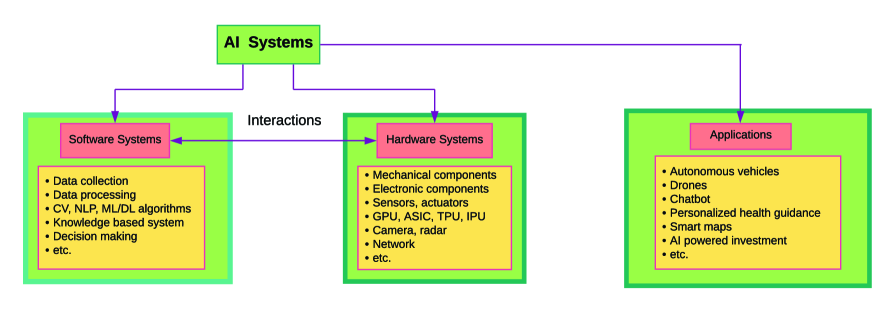
Figure 1: Illustration of AI system framework that consists of software and hardware systems, and examples of AI applications.

1.3 The Importance of AI Reliability

For any system, reliability is often of interest because failure events can lead to safety concerns. Failures of AI systems can lead to economic loss and even, in some extreme cases, lead to loss of life. For example, a failure in the autopilot system of an autonomous car can lead to an accident with loss of life. Thus, reliability is critical, especially for autonomous systems.

To provide some concrete examples, we use the AI incident cases reported on the website AIIncidentDB database (2021), which gathers news entries from various sources. Among those 126 incidents reported up to date, we found 72 incidents can be related to reliability events. Figure 2 plots the counts for the AI application sectors, and for the AI systems and technologies, based on the 72 reliability-related cases. The figure shows AI applications are popular in many sectors and various AI systems and technologies are applied. Despite the prevalence, we also notice that 29 incidents involve deaths or injuries among those 72 events, which shows reliability issues can lead to serious loss.

From another point of view, the large-scale deployment of AI technologies requires public trust. High reliability is one important aspect for winning the trust of the consumers, which requires reliability demonstration. The importance of the reliability of AI systems has been highlighted by several authors. For example, jenihhin2019challenges reviewed the challenges of reliability assessment and enhancement in autonomous systems. athavale2020ai discussed the trends in AI reliability in safety-critical autonomous systems on the ground and in the air.

The proper demonstration of AI system reliability requires capturing real-world scenarios together with real failure modes. Thus, data collections are essential for demonstrating AI reliability, and statistics can play an important role in such efforts. After obtaining AI reliability data, the statistical modeling and analysis, and reliability predictions can be done. The data can also be used to identify causes of reliability issues and thus one can improve the design of the AI systems for better reliability, which is challenging but provides opportunities for statistical reliability research.

AI reliability falls within the larger scope of AI safety and AI assurance, the importance of which has been emphasized in many existing research papers. Amodeietal2016 outlined concrete problems in AI safety research, and batarseh2021survey provided a comprehensive review of research on AI assurance. Thus, from a larger scope, AI reliability is an important aspect of AI assurance, where research efforts need to be devoted on.

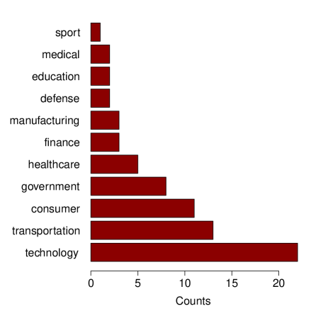
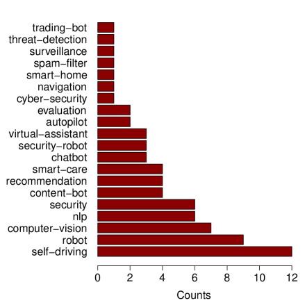
(a) AI Application Sectors	(b) AI Systems/Technologies

Figure 2: Counts for the AI application sectors (a) and for the AI systems/technologies (b), based on the 72 reliability-related cases in the AI Incident database.

1.4 Overview

The rest of the paper is organized as follows. Section 2 describes a general “SMART” statistical framework for AI reliability. Section 3 briefly describes the common methods used in traditional reliability methods and how they can be linked to AI reliability studies. Section 4 discusses new challenges in statistical modeling and analysis of AI reliability, and several specific topics for statistical research with illustrative examples. Section 5 discusses how to use the design of experiments approaches in data collection for AI reliability studies and improvement. Section 6 contains some concluding remarks.

2 AI Reliability Framework and Failure Analysis

In this section, we introduce the “SMART” framework for AI reliability study, which contains five components. Here, the acronym “SMART” comes from the first letter of the five components below.

• Structure of the system:Understanding the system structure is a fundamental step in the AI reliability study. • Metrics of reliability:Appropriate metrics need to be defined for AI reliability so that data can be collected over those metrics. • Analysis of failure causes:Conducting failure analysis to understand how the system fails (i.e., failure modes) and what factors affect the reliability. • Reliability assessments:Reliability assessments of AI systems include reliability modeling, estimation, and prediction. • Test planning:Test planning methods are needed for efficient reliability data collection.

The first three points are covered in Section 2. The traditional and new framework for AI reliability assessment is covered in Sections 3 and 4, respectively. Test planning is covered in Section 5.

2.1 System Structures

For AI systems (e.g., autonomous vehicles), we can conceptually divide the overall system into hardware systems and software systems. Figure 1 lists some commonly seen hardware and software systems. In addition to the typical hardware in a product (e.g., the mechanical devices in a vehicle), the hardware used for AI computing can include central processing unit (CPU), application-specific integrated circuit (ASIC), graphics processing unit (GPU), tensor processing unit (TPU), and intelligence processing unit (IPU). There are also various types of cameras, sensors, and devices that are used for collecting images, sounds, and other data formats that feed into the AI system. The hardware can also include network infrastructure as wireless communication is common for AI systems.

The core of many software systems consists of machine learning/deep learning (ML/DL) based algorithms and other rule-based algorithms. The algorithms include image recognition and speech recognition, CV, NLP, and classifications. The text cloud in Figure 3(a) shows the variety of algorithms used in the reliability-related cases reported in the AI Incident database. In addition to the core ML/DL algorithms, the software system can also include data collection, processing, and decision-making components.

Many algorithms are based on DL models. The widely used DL algorithm structures include deep neural network (DNN), convolutional neural network (CNN), recurrent neural network (RNN), and reinforcement learning (RL). An introduction to those neural network structures can be found in Goodfellow-et-al-2016. Transfer learning also has been used in AI systems. A comprehensive introduction of transfer learning is available in pan2009survey.

Hardware reliability is in general well studied, or there are mature methods for testing and assessing hardware reliability. Thus, the focus of AI reliability, different from traditional reliability studies, is on the software system. More specifically, it is on the reliability of those ML/DL algorithms. Compared to hardware reliability, software reliability is typically more difficult to test, which brings challenges to the research and development of reliable AI systems.

In addition to the hardware and software systems, there are two other factors to consider as the AI system structure: the hardware-software interaction, and the interaction of the system to the operating environment. The new challenges are on how hardware error affects the software and are there algorithms or architectures more robust to hardware failures. AI systems are typically trained or developed for the use of a certain operating environment. When the operating environment changes, it is likely that the AI systems will encounter errors. Thus system structures that can be adaptive to the operating environment will make the system more reliable.

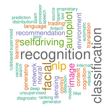
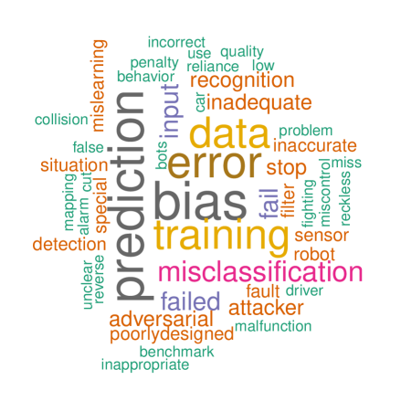
(a) Algorithms	(b) Failure Causes

Figure 3: Text clouds for the algorithms used in the AI systems (a) and for the failure causes (b), based on the 72 reliability-related cases in the AI Incident database after removing entries with unknown algorithms and causes.

2.2 Definition of AI Reliability and Metrics

The usual definition of reliability is the probability of a system performing its intended functions under expected conditions. Reliability is closely related to robustness and resilience, but the focus is on the time dimension. There is little work that formally defines the reliability of AI systems. For AI systems, because the software system is of major concern, the definition of AI reliability is more toward the software part. kaur2014software defined the reliability of software as “the probability of the failure-free software operation for a specified period of time in a specified environment.”

There are three key elements in the definition of reliability, “failure”, “time”, and “environment”. The failure events of an AI system can be mostly related to software errors, in addition to the failure of hardware. For hardware failures, hanif2018robust discussed that AI hardware failures are related to soft errors, aging, process variation, and temperature. For software failures, software errors and interruptions are generally considered as failure events. For example, the occurrence of a disengagement event is considered as a failure of the system for AV (e.g., MinHongKingMeeker2020).

The time scale in AI reliability can be different for different structure levels or AI applications. For AI systems, the system use cycles instead of the usual calendar time may be a more appropriate time scale. For algorithms implemented in AI applications, it is more reasonable to use the number of algorithm evaluations, or the number of calls to the AI algorithms as the time scale. In the autonomous vehicle application, the miles driven is a more appropriate proxy of the time scale.

The environment includes the physical environment for hardware systems such as temperature, humidity and vibration, and the environment defined by the training dataset. For example, if there is an object that is not in the training dataset, the AI system may not be able to recognize it, and thus the object is beyond the intended operating environment. The operating environment defined by the software system is usually more important for AI reliability.

Metrics are needed to characterize reliability for AI systems such as failure rate, event rate, error rate, etc. For hardware, the bit flip error rate has been used in literature. Both hanif2018robust and kundu2021special mentioned the measurement of bit flip fault on hardware. kundu2021special further connected the bit flip fault to model accuracy. Thus, one may use the rate of bit flip faults to explain the overall model accuracy drop.

The metrics for software related failures are more complicated. The measurement of the reliability of an AI algorithm is associated with the performance of the AI algorithm. Most AI algorithms are designed to solve problems of classification, regression, and clustering, etc. bosnic2009overview used prediction accuracy from ML algorithms as a reliability measure. zhang2019case defined statistical robustness from three aspects: sampling quality, convergence diagnostic, and goodness of fit. Jhaetal2019 introduced an attribution-based confidence metric for DNN, which can be computed without the training dataset. Overall, there are many metrics available at the algorithm level, but in general lack universal metrics for algorithm reliability. For the system level, the event rate is suitable for a wide range of applications.

2.3 Failure Modes and Affecting Factors

The failure modes in the hardware level have two main types, hard failures and transient failures. Examples of hard failures include the faults in high-performance computing (HPC) clusters and cloud-computing systems (e.g., 6270765), which provide infrastructure for many AI applications. The soft or transient failure refers to the failure that will only happen when one signal of the system exceeds the threshold. For example, Goldsteinetal2020 studied the effects of transient faults on the reliability of compressed CNN. Hardware failures can also include the network infrastructure failure because the network is an important component for many AI systems. Thus, network failure is also a form of hardware failures. Traditional factors such as the physical environment (e.g., temperature, humidity, vibration), and product use rate affect the hardware systems.

There can be various reasons for the failures at the software level. Figure 3(b) shows the text cloud for the potential failure causes for the reliability-related cases reported in the AI Incident database. As we can see from the plot, typical causes are prediction errors, data quality, model bias, adversarial attacks (AA), and so on.

Many prediction errors are caused by distribution shift. Distribution shift usually means the operating environment is different from the training-set environment. For example, MARTENSSON2020101714 studied the reliability of DL models on the out-of-distribution MRI data. AA can be a critical issue for reliability. In AA, a small permutation to the data is applied to make the model prediction inaccurate, leading to reliability incident. For example, 220580 provided an example of the AA on object detection tasks. Data quality can also lead to software failures. If the data that are fed into the algorithm come with noises, are contaminated, or are from faulty sensors, failures can also occur. For example, ma2020artificial discussed sensor data quality on AI reliability.

Failure causes can also be different based on the algorithm type (e.g., CNN, RNN). Certain algorithms may be less prone to failure than others. Compared to hardware issues, software issue is more of a concern for AI reliability. For example, Lvetal2018 performed an exploratory analysis of the causes of disengagement events using the California driving test data and found that software issues were the most common reasons for failure events.

Based on the above discussion, the factors that can affect AI reliability can fall into three categories: operating environment, data, and model (i.e., algorithm). Figure 4 shows the Venn diagram for the three factors that affect AI reliability, which will be further discussed in Section 4.1. The interactions of the three factors (e.g., data-model interaction) complicate the reliability modeling problems and provide many opportunities for statistical research.

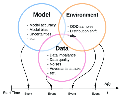
Figure 4: Illustration of AI reliability affecting factors and AI reliability modeling framework.

2.4 AI Reliability Data and Existing Analyses

Reliability assessment of AI systems requires data that are collected over the reliability metrics. Depending on the reliability metric, different kinds of data can be collected. The existing work on AI reliability data analysis is sparse.

At the system level, the reliability data is usually in the format of time-to-event data. The availability of reliability data for autonomous systems is limited due to the sensitive nature of reliability data. The CAdriving (2020) has made the reliability testing data of AV available to the public. For the California driving data, exploratory analyses of the data include dixit2016autonomous, favaro2018autonomous, Lvetal2018, and Boggsetal2020. For further modeling, banerjee2018hands used linear regression models, Merkel2018 analyzed the aggregated counts of events, and Zhaoetal2019 used the Bayesian method to estimate event rates. MinHongKingMeeker2020 used the large-scale field-testing data and conducted a statistical analysis of AI reliability and especially for AV reliability. In addition to the California driving data, the AIIncidentDB (2021) provided a database that collects AI incidents mainly from news reports.

At the component level, the AI reliability data depend on the actual applications of the AI algorithm. Thus, various types of data can be collected for both hardware and software components. Bosioetal2019 conducted a reliability analysis of deep CNN under fault injections. michelmore2019uncertainty designed a statistical framework to evaluate the safety of DNN controllers and assessed the safety of AV. Goldsteinetal2020 studied the impact of transient faults on the reliability of compressed deep CNN. AlshemaliKalita2020 provided a review of methods for improving the reliability of NLP. zhao2020safety proposed a safety framework based on Bayesian inference for critical systems using DL models. In summary, a general modeling framework for reliability of AI systems needs to be developed.

3 The Roles of Traditional Reliability

3.1 Traditional Reliability Analysis

Traditional reliability analysis mainly uses the time-to-event data, degradation data, and recurrent events data to make reliability predictions. The classical methods of reliability data analysis can be found in, for example, Nelson1982, lawless2003, and MeekerEscobarPascual2021. The area of reliability analysis has gone through many changes due to technology development, especially due to sensory prevalence, and new opportunities have been outlined in MeekerHong2014, and HongZhangMeeker2018. In this section, we give a brief introduction to traditional reliability analysis methods and link them to AI reliability data analysis.

Time-to-event data usually provide the failure time for failed units and time in service for surviving units. For illustration, Figure 5(a) shows the event plot for the GPU failure times in years as reported in Ostrouchovetal2020, in which both failures and censored observations are involved. For AI reliability, the failure time can be the time to an incident that leads to a system failure caused by the AI systems. The incident can be either from hardware or software.

Parametric models such as the Weibull and lognormal distributions are widely used to model the time-to-event data. Accelerated failure time models are often used to model covariate information. For failure-time data, suppose we have $n$ units of a product, and we denote $t_{i}$ as the lifetime or time in service of unit $i$ and $\delta_{i}$ the censoring indicator. Here, $\delta_{i}=1$ if unit $i$ failed and $\delta_{i}=0$ otherwise. The parametric lifetime model usually assumes the random variable lifetime $T$ follows a log-location-scale family of distributions, which includes the commonly used Weibull and lognormal distributions. The cumulative distribution function (cdf) and probability density function (pdf) of $T$ are,

$$F(t;{\boldsymbol{\theta}})=\Phi\left[\frac{\log(t)-\mu}{\sigma}\right],\quad\textrm{and}\quad f(t;{\boldsymbol{\theta}})=\frac{1}{\sigma t}\phi\left[\frac{\log(t)-\mu}{\sigma}\right],$$

respectively. Here, $\mu$ is the location parameter, $\sigma$ is the scale parameter, and ${\boldsymbol{\theta}}=\left(\mu,\sigma\right)^{\prime}$. For lognormal distribution, we can replace $\Phi$ and $\phi$ with the standard normal cdf $\Phi_{\textrm{nor}}$ and pdf $\phi_{\textrm{nor}}$, respectively. For the Weibull distribution, we can replace $\Phi$ and $\phi$ with $\Phi_{\textrm{sev}}(z)=1-\exp[-\exp(z)]$ and pdf $\phi_{\textrm{sev}}(z)=\exp[z-\exp(z)]$, respectively.

For failure-time data, the reliability function is defined as $R(t;{\boldsymbol{\theta}})=\Pr(T>t)$. The likelihood function can be written as,

$$L({\boldsymbol{\theta}})=\prod_{i=1}^{n}f(t_{i};{\boldsymbol{\theta}})^{\delta_{i}}\left[1-F(t_{i};{\boldsymbol{\theta}})\right]^{(1-\delta_{i})}.$$ (1)

The maximum likelihood estimates can be obtained by finding the value of ${\boldsymbol{\theta}}$ that maximizes (1). The inference of the reliability of the product is based on the estimated reliability function $R(t;\widehat{{\boldsymbol{\theta}}})$.

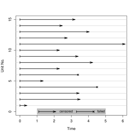
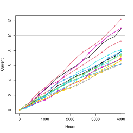
(a) GPU Failure-time Data	(b) Laser Degradation Data

Figure 5: Examples of failure-time data  (a) and degradation data (b). The horizontal line in (b) shows the failure threshold.

Degradation data measure the performance of the system over time. When the performance deterioration reaches a pre-defined failure threshold, a failure occurs. For illustration, Figure 5(b) plots the degradation paths for a group of laser units, in which the performance deterioration is measured by the percentage of current increase. Performance degradation can also occur for AI models over time. For example, the performance of AI-based models can deteriorate over time after deployment in the field due to conditional changes. For computing hardware, the soft error rate can increase over time for AI systems.

For degradation data, the two widely used classes of models are the general path models (e.g., LuMeeker1993, BagdonaviciusNikulin2001, and BaeKuoKvam2007) and stochastic models. The stochastic models include the Winer process (e.g., Whitmore1995), gamma process (e.g., LawlessCrowder2004), and the inverse Gaussian process (e.g., YeChen2014). Covariate information is often incorporated through regression models.

Here we give a brief introduction to the general path model (GPM), which was originally proposed by LuMeeker1993. Suppose the degradation level is $\mathcal{D}(t)$ at time $t$. We consider a failure occurred for a unit if its $\mathcal{D}(t)$ reaches a failure-definition level $\mathcal{D}_{f}$. Then the failure time is the first time at which $\mathcal{D}_{f}$ is reached, that is, $t_{\mathcal{D}}=\min\{t:\mathcal{D}(t)\text{ reaches }\mathcal{D}_{f}\}$. The basic idea of GPM is to find a parametric model that fits all paths well. Let $y_{ij}$ be the degradation measurement for unit $i$ at time $t_{ij}$, $j=1,\dots,n_{i}$ and $i=1,\dots,n$. Here, $n$ is the number of units, and $n_{i}$ is the number of measurements from unit $i$. Then the degradation path can be modeled as,

$$y_{ij}=\mathcal{D}(t_{ij};\boldsymbol{\alpha},{\boldsymbol{\gamma}}_{i})+\epsilon_{ij},$$

where $\boldsymbol{\alpha}$ represents the vector of fixed-effect parameters and ${\boldsymbol{\gamma}}_{i}$ represents the vector of random effects for unit $i$. The random effects are assumed to follow multivariate normal distribution $\textrm{MVN}({\boldsymbol{0}},{\boldsymbol{\Sigma}})$ with pdf $f_{\textrm{MVN}}(\cdot;{\boldsymbol{\Sigma}})$. The error is assumed to be independent and follows normal distribution $\epsilon_{ij}\sim\textrm{N}(0,\sigma_{\epsilon}^{2})$. Denote the parameter in model as ${\boldsymbol{\theta}}=\left\{\boldsymbol{\alpha},{\boldsymbol{\Sigma}},\sigma_{\epsilon}^{2}\right\}$. For the estimation of ${\boldsymbol{\theta}}$, we can obtain the maximum likelihood estimates by maximizing the likelihood function,

$$L({\boldsymbol{\theta}}|\text{Data})=\prod_{i=1}^{n}\int_{-\infty}^{\infty}\left[\prod_{j=1}^{n_{i}}\frac{1}{\sigma_{\epsilon}^{2}}\phi_{\textrm{nor}}\left(z_{ij}\right)\right]\times f_{\textrm{MVN}}({\boldsymbol{\gamma}}_{i};{\boldsymbol{\Sigma}})d{\boldsymbol{\gamma}}_{i},$$

where $z_{ij}=\left[y_{ij}-\mathcal{D}(t_{ij};\boldsymbol{\alpha},{\boldsymbol{\gamma}}_{i})\right]/\sigma_{\epsilon}^{2}$.

The cdf of the failure time $T$ is, $F_{T}(t;{\boldsymbol{\theta}})=\Pr(T\leq t)=\Pr[\mathcal{D}(t)\geq\mathcal{D}_{f}]$, for an increasing path. Except for some simple degradation paths, in most situations $F_{T}(t;{\boldsymbol{\theta}})$ does not have a closed-form expression. Numerical methods such as numerical integration and simulation can be used to compute the cdf of $T$. The inference of the reliability is made based on $\widehat{F}_{T}(t;{\boldsymbol{\theta}})$.

Recurrent events occur when a system can experience the same events repeatedly over time. For AI systems, failure-time data and degradation data mainly result from hardware failures, while recurrent events data mainly come from software failures. Recurrent events occur in AI systems such as the disengagement events in autonomous vehicles as analyzed in MinHongKingMeeker2020. Although we defer the details of the dataset to Section 3.3, Figure 6(a) plots the recurrence of the disengagement events over time for AV units.

The recurrent events data are often modeled by the event intensity models or mean cumulative functions with regression models that are often used to incorporate covariates. Nonhomogeneous Poisson process (NHPP) and renewal process are widely used (e.g., YangZhangHong2013, and HongLiOsborn2015). LindqvistElvebakkHeggland2003 proposed the trend-renewal process, which can include the NHPP and renewal process as special cases.

Here we briefly introduce the NHPP model. Denote $N(t)$ as the number of events occurred in $(0,t]$ and $N(s,t)$ as the number of events in time $(s,t]$. For a Poisson process, the number of recurrences in $(s,t]$ follows a Poisson distribution with parameter $\Lambda(s,t)$. That is,

$$\Pr[N(s,t)=d]=\frac{\Lambda(s,t)^{d}}{d!}\exp[-\Lambda(s,t)],\quad d=0,1,\cdots.$$

Here, $\Lambda(s,t)$ represents the cumulative intensity function between time $s$ and $t$. That is, $\Lambda(s,t)=\int_{s}^{t}\lambda(u)du$, $\Lambda(t)=\Lambda(0,t)$, and $\lambda(u)$ is a positive recurrence rate. For NHPP, the intensity function is non-constant and it can be assumed as a known function form with unknown parameters. For example, the power-law function,

$$\lambda(t;{\boldsymbol{\theta}})=\frac{\beta}{\eta}\left(\frac{t}{\eta}\right)^{(\beta-1)},\quad\beta>0,\eta>0,$$

is a commonly used form for the intensity function with parameter ${\boldsymbol{\theta}}=(\beta,\eta)^{\prime}$.

For the parameter estimation, we can use the maximum likelihood method. Suppose we have $n$ units, and the event times for unit $i$ is $t_{ij}$. The event time are ordered as $0<t_{i1}<t_{i2}<\dots<t_{in_{i}}<\tau_{i}$. Here, $n_{i}=N(\tau_{i})$ is the number of events and $\tau_{i}$ is the last observation time for unit $i$. Then the likelihood is,

$$L({\boldsymbol{\theta}})=\prod_{i=1}^{n}\left[\prod_{j=1}^{n_{i}}\lambda(t_{ij};{\boldsymbol{\theta}})\right]\exp\left[-\Lambda(\tau_{i};{\boldsymbol{\theta}})\right],$$

with $\prod_{j=1}^{0}\left(\cdot\right)=1$. The statistical inference is based on the estimated intensity function, $\lambda(t;\widehat{{\boldsymbol{\theta}}})$.

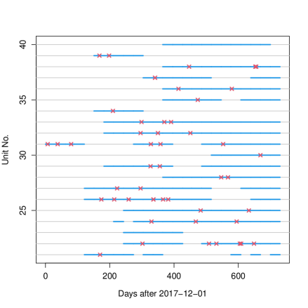
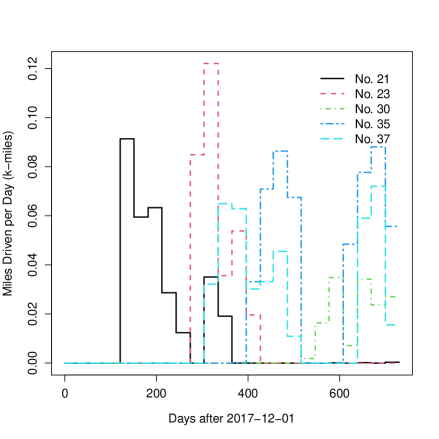
(a) Disengagement Events	(b) Miles Driven per Day

Figure 6: The recurrent events data with the crosses showing the event times and the blue segments showing the active months for Waymo (a), and plot of the mileage as a function of time for five representative units (b).

3.2 Relationship with Software Reliability

Software reliability is an area of traditional reliability that is closely related to AI reliability. In modeling software reliability, usually a software reliability growth model (SRGM) based on NHPP is built. The assumption is that the faults of software should be fixed through testing. There are basically two different classes of traditional SRGMs based on the shape of cumulative failures against time as described in Wood1996: S-shaped and concave. In Table 1, the Weibull SRGM is concave, and the Gompertz SRGM is S-shaped. SRGMs can be used in modeling the reliability of AI algorithms. For example, Merkel2018 used the Gompertz model and Musa-Okumoto model for the California AV disengagement data, and MinHongKingMeeker2020 developed spline models for SRGM. In addition, ZhaiYe2020 considered the reliability growth test of unmanned aerial vehicles. NafreenFiondella2021 proposed a family of software reliability models with bathtub shapes that balance model complexity and predictive accuracy.

Different from traditional software, in which the operating environment is relatively stable and the system is less affected by the environment, the performance of AI algorithm depends on operating environment to a larger extent. In addition, there may be intrinsic errors inside the AI algorithm that can not be removed. Thus, the assumption in traditional software reliability, that the reliability of software goes to 1 as testing time goes to infinity, may not hold for AI reliability. To fix this, bastani1990assessment used two independent Poisson processes to model the feature of reliability of AI, in which the failure rate decreases through time in one Poisson process, and the failure rate is fixed in the other Poisson process. Such an idea can be further extended to model more complicated reliability AI problems.

There are also NHPP-based software reliability models that were developed for the fault intensity function and the mean cumulative function (song2017threee). Here we briefly discuss those ideas. As introduced in pham2019generalized, let $\lambda(t)$ be the fault intensity function, $\Lambda(t)$ be the mean cumulative function, and $N(t)$ be the number of faults. The mean cumulative function $\Lambda(t)$ is modeled as,

$$\frac{d\Lambda(t)}{dt}=\lambda(t)[N(t)-\Lambda(t)].$$

Further, the $\lambda(t)$ term is multiplied by a random effect that represents the uncertainty of the system fault detection rate in the operating environments. The paper also takes the uncertainty of the operating system into consideration, and lets $\lambda(t)$ be a stochastic process, which considers both dynamic additive noise model and static multiplicative noise model for $\lambda(t)$. These models, however, have not been applied in modeling an AI system yet.

Table 1: List of commonly used parametric forms for SRGM.

Model	$\Lambda_{0}(t;{\boldsymbol{\theta}})$	Parameters
Musa-Okumoto	$\theta_{1}^{-1}\log(1+\theta_{2}\theta_{1}t)$	${\boldsymbol{\theta}}=(\theta_{1},\theta_{2})^{\prime}$
		$\theta_{1}>0,\theta_{2}>0$
Gompertz	$\theta_{1}\theta_{3}^{\theta_{2}^{t}}-\theta_{1}\theta_{3}$	${\boldsymbol{\theta}}=(\theta_{1},\theta_{2},\theta_{3})^{\prime}$
		$\theta_{1}>0,0<\theta_{2},\theta_{3}<1$
Weibull	$\theta_{1}[1-\exp(-\theta_{2}t^{\theta_{3}})]$	${\boldsymbol{\theta}}=(\theta_{1},\theta_{2},\theta_{3})^{\prime}$
		$\theta_{1}>0,\theta_{2}>0,\theta_{3}>0$

3.3 Applications of Traditional Methods in AI

In this section, we provide an illustration on how traditional reliability methods can be applied in modeling AI reliability. MinHongKingMeeker2020 analyzed the disengagement events data from AV testing program overseen by the California Department of Motor Vehicles (DMV). A disengagement event happens when the AI system and/or the backup driver determines that the driver needs to take over the driving. Disengagement events can be seen as a sign of “not reliable enough” of the AV. The program provides data on disengagement event time points and the monthly mileage driven by the AVs.

MinHongKingMeeker2020 analyzed disengagement event data from manufacturers Waymo, Cruise, PonyAI and Zoox for the period from December 1, 2017 to November 30, 2019. Following the notation in MinHongKingMeeker2020, let $n$ be the number of AV testing vehicles in the fleet of a manufacturer, and let $t_{ij}$ be the $j$th event time for unit $i$, $i=1,\ldots,n,j=1,\ldots,n_{i}$. Here, $t_{ij}$ records the number of days since December 1, 2017, and $n_{i}$ is the number of events for unit $i$. The total follow-up time is $\tau=730$ days. Let $x_{i}(t),0<t\leq\tau$, be the mileage driven for unit $i$ at time $t$. The unit of $x_{i}(t)$ is k-miles (i.e., 1000 miles). The daily average of monthly mileage was used for $x_{i}(t)$, and $x_{i}(t)$ can be represented as $x_{i}(t)=\sum_{l=1}^{n_{\tau}}x_{il}{\mathds{1}}{(\tau_{l-1}<t\leq\tau_{l})}.$ Here, $n_{\tau}=24$ is the number of months in the follow-up period, $x_{il}$ is the daily mileage for unit $i$ during month $l$, $\tau_{l}$ is the ending day since the starting of the study for month $l$, and ${\mathds{1}}{(\cdot)}$ is an indicator function. Let $\boldsymbol{x}_{i}(t)=\{x_{i}(s):0<s\leq t\}$ be the history for the mileage driven for unit $i$. Figure 6 shows a visualization of a subset of the recurrent events data from manufacturer Waymo. In particular, Figure 6(a) shows the observed window and events of 20 AVs, and Figure 6(b) shows the corresponding driven mileage of five AV units.

As described in Section 3.1, the NHPP model is usually used to describe recurrent event rate. The event intensity function for unit $i$ is modeled as,

$$\lambda_{i}[t;x_{i}(t),{\boldsymbol{\theta}}]=\lambda_{0}(t;{\boldsymbol{\theta}})x_{i}(t).$$

Here, $\lambda_{0}(t;{\boldsymbol{\theta}})=\lambda_{0}(t)$ is the baseline intensity function (BIF) with parameter vector ${\boldsymbol{\theta}}$. Because $x_{i}(t)$ is the mileage driven, $\lambda_{i}[t;x_{i}(t),{\boldsymbol{\theta}}]$ is the mileage-adjusted event intensity, the BIF can be interpreted as the event rate per k-miles at time $t$ when $x_{i}(t)=1$. The baseline cumulative intensity function (BCIF) is $\Lambda_{0}(t;{\boldsymbol{\theta}})=\Lambda_{0}(t)=\int_{0}^{t}\lambda_{0}(s;{\boldsymbol{\theta}})ds$. Note that $\Lambda_{0}(0;{\boldsymbol{\theta}})=0$ and $\Lambda_{0}(t;{\boldsymbol{\theta}})$ is a non-decreasing function of $t$. The BCIF $\Lambda_{0}(t)$ can be interpreted as the expected number of events from time 0 to $t$ when $x(t)=1$ for all $t$. The CIF for unit $i$ is $\Lambda_{i}[t;x_{i}(t),{\boldsymbol{\theta}}]=\int_{0}^{t}\lambda_{0}(s;{\boldsymbol{\theta}})x_{i}(s)ds$.

Commonly used parametric models for NHPP, such as those listed in Table 1, can be applied to model $\Lambda_{0}(t)$. Other than the parametric model, MinHongKingMeeker2020 also proposed a more flexible nonparametric spline method to estimate the BCIF of NHPP. In the spline model, the BCIF is represented as a linear combination of spline bases. That is,

$$\Lambda_{0}(t;{\boldsymbol{\theta}})=\sum_{l=1}^{n_{s}}\beta_{l}\gamma_{l}(t),\quad\beta_{l}\geq 0,\,l=1,\ldots,n_{s},$$

Here, ${\boldsymbol{\theta}}=(\beta_{1},\ldots,\beta_{n_{s}})^{\prime}$ is the vector for the spline coefficients, $\gamma_{l}(t)$’s are the spline bases, and $n_{s}$ is the number of spline bases. Taking the derivative with respect to $t$, the BIF is,

$$\lambda_{0}(t;{\boldsymbol{\theta}})=\frac{d\Lambda_{0}(t;{\boldsymbol{\theta}})}{dt}=\sum_{l=1}^{n_{s}}\beta_{l}\frac{d\gamma_{l}(t)}{dt}.$$

Because of the constraints that $\Lambda_{0}(0;{\boldsymbol{\theta}})=0$ and that $\Lambda_{0}(t;{\boldsymbol{\theta}})$ is a non-decreasing function of $t$, I-splines with degree 3 is used (e.g., Ramsay1988). Each I-spline basis takes value zero at $t=0$ and is monotonically increasing. By taking non-negative coefficients (i.e., $\beta_{l}\geq 0$), a non-decreasing $\Lambda_{0}(t;{\boldsymbol{\theta}})$ is obtained. Numerical algorithms are used for parameter estimation.

For illustration, Figure 7(a) shows the expected versus the observed number of events for Waymo using the four parametric models and the spline model. The expected number of events is computed based on the specific model with the adjustment for the mileage history from all units. The spline curve follows closely with the data points in Figure 7(a), and the 95% pointwise confidence intervals contain the data points, indicating that the spline model fits the data well. The less flexible parametric models can not track the data well when there is a curvature in the observed cumulative events curve, but the estimation is also not bad.

Figure 7(b) shows the estimated BIFs using the best parametric model for the four manufacturers. For Waymo, Cruise, and Pony AI, the estimated BIFs decrease as time increase, indicating that there are improvements in the AV reliability through time for these three manufacturers. However, for Zoox, although at the starting point, the estimated BIF is just above 0.5, which is a lot better compared with the estimated BIF of PonyAI, it keeps unchanged through time. This pattern indicates that there are not many improvements in the AV reliability for Zoox.

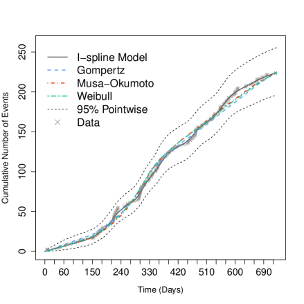
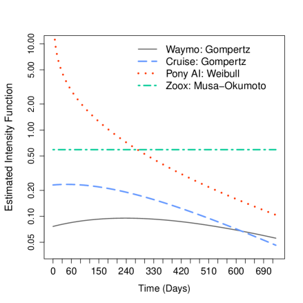
(a) Waymo	(b) Estimated BIF

Figure 7: Plots of the expected versus the observed number of events for manufacturer Waymo based on the spline model and parametric models, together with the 95% pointwise confidence intervals based on the spline model (a), and the estimated BIFs from the best parametric models for the four manufacturers (b).

4 Challenges in Statistical Analysis of AI Reliability

4.1 A Framework for AI Reliability Modeling

As discussed in Section 2, an AI system can fail due to hardware and software reasons. Because hardware failures can be well tackled by the traditional reliability framework, we focus on the software aspect of the problem. For the software components, ML/DL algorithms are widely used in many AI systems. As discussed in Section 2.3, the three factors mainly contribute to failure events are environment, data, and model (i.e., algorithm).

As a framework to model AI reliability, we focus on interruptive events, which are caused by operating environment, data, and models, that can lead to software errors. We define those events as failure events. Because reliability focuses the performance over the time, we can link the failure events to the time process. Assuming the arrival of such events follows a stochastic process (e.g., NHPP), we can further link the events to reliability prediction. Then, the traditional methods in reliability can all be applied. The idea of modeling for AI reliability is illustrated in Figure 4, in which the counting process $N(t)$ represents the event process.

To introduce the modeling framework, we define some more notations. Suppose there are $k$ types of interruptive events and the arrival of those events follows a counting process $N_{j}(t)$ with intensity function $\lambda_{j}[t;\boldsymbol{x}(t)]$, which depends on covariate vector $\boldsymbol{x}(t)$. Here, $\boldsymbol{x}(t)$ is a general vector that contains external information such as the operating environment (e.g., the occurrence of distribution shift), low quality of input data , data noise, and arrival of adversarial attacks (AA).

The probability of such an interruptive event resulting in a failure event is modeled as $p_{j}({\boldsymbol{z}})$. Here, ${\boldsymbol{z}}$ is a general vector that summarizes the internal reliability properties of the AI systems. For example, ${\boldsymbol{z}}$ may contain information on the system’s ability of out-of-distribution (OOD) detection, its robustness to low quality data and AA, and its ability to generate highly accurate prediction with low uncertainty. The probability $p_{j}({\boldsymbol{z}})$ can be modeled as,

$$p_{j}({\boldsymbol{z}};{\boldsymbol{\beta}}_{j})=\frac{\exp({\boldsymbol{z}}^{\prime}{\boldsymbol{\beta}}_{j})}{1+\exp({\boldsymbol{z}}^{\prime}{\boldsymbol{\beta}}_{j})},$$

through parameter ${\boldsymbol{\beta}}_{j}$, $j=1,\cdots,k$. Thus the overall intensity for the counting process $N(t)$ for the failure events is,

$$\lambda[t;\boldsymbol{x}(t),{\boldsymbol{z}}]=\sum_{j=1}^{k}\lambda_{j}[t;\boldsymbol{x}(t)]\cdot p_{j}({\boldsymbol{z}};{\boldsymbol{\beta}}_{j}).$$ (2)

Based on model (2), reducing $p_{j}({\boldsymbol{z}})$ can improve the reliability of the AI systems. The research remaining is to model the event process, which depends on the three factors and their interactions.

Here we discuss some characteristics of the three factors. For the operating environments, one common contribution to failure events is that the operating environments are different from the training environments, which is referred to as OOD samples. For example, a new object appears and the AI algorithm can not recognize it. If the algorithm fails to detect the OOD samples in making a prediction, an incorrect decision is likely to be made, and potentially leads to errors. Thus, OOD detection, and being able to make an appropriate adaptation for OOD samples are important in improving AI reliability.

Also, the quality of the training data is highly related to the performance of the algorithm. Data with errors, for example, caused by sensor mal-function, can lead to errors in prediction. Another aspect of data quality is related to the data bias/imbalance issue, which is more of importance for many classification algorithms used in AI systems. The effect of data quality on the performance of the AI systems is coupled with the algorithm. Thus, it is of interest to study how data and algorithms affect model accuracy. AA can be viewed as a special kind of “data quality” issue, in which one purposely uses problematic inputs to the algorithm so that the AI system will fail to generate the correct output. The robustness of an algorithm from AA is a key to the reliability of the AI system.

Most AI system depends on the accuracy of the prediction powered by ML/DL algorithms. The adopted algorithm needs to provide accuracy high enough on the training set so that it can be used in practice. Thus, it is important to study the relationship between reliability and model accuracy. In addition, the prediction made by the algorithm is associated with uncertainty. High uncertainty can lead to less reliable performance, and quantifying uncertainty in prediction is also an important task.

In the following sections, we give a brief introduction to OOD detection, the modeling of data quality and AI algorithms, AA, and model accuracy and uncertainty quantification, with some illustrative examples.

4.2 Out-of-Distribution Detection

The OOD observations in the data never appear in the training set. In classification problems, many ML tasks assume the labels in the test set all appear in the training set. However, it is possible that we encounter a new class in the test dataset. For example, we want to use the images of hind legs of the frogs caught in southeastern Asian rain forests to predict the species of the frogs. According to Lambertzetal2014, it is possible that these frogs belong to a new species that has never been discovered.

There are various existing methods for detecting OOD samples for technologies used in AI. lee2018simple used the intermediate-layer data of one pre-trained CNN to classify the outliers in both training and testing set. The intermediate-layer data of the CNN are assumed to have a multivariate normal distribution and outliers are treated to have large Mahalanobis distance. liang2017enhancing used temperature scaling to distill the knowledge in multiple pre-trained DNN models of the same prediction task to classify the outliers data. winkens2020contrastive used confusion log-probability to measure the similarity of the samples. Those OOD samples will have a low confusion log-probability. Other popular methods for detecting OOD samples include representations from classification networks (sastry2020detecting), alternative training strategies (lee2017training), Bayesian approaches (blundell2015weight), and generative and hybrid models (choi2018waic).

Here, we give a concrete application for an illustration of OOD detection. Given a pre-trained CNN-based network, let $\boldsymbol{x}_{i}$ and $y_{i}$, $i=1,\ldots,n$, be the inputs and outputs of the network, respectively. Here, $n$ is the number of samples. Let $j$ be the class index, and $n_{j}$ be the number samples within class $j$. The current total number of classes is denoted by $k$.

We use $f(\boldsymbol{x})$ to denote the output of the penultimate layer (the layer before the activation function) of the neural network. Then we assume that $f(\boldsymbol{x})$ given class $j$ follows a multivariate normal distribution. That is, $f(\boldsymbol{x})|y=j\sim\textrm{MVN}(\boldsymbol{\mu}_{j},{\boldsymbol{\Sigma}})$, where the mean and variance-covariance matrix are estimated as,

$$\widehat{\boldsymbol{\mu}}_{j}=\frac{1}{n_{j}}\sum_{i:\,y_{i}=j}f(\boldsymbol{x}_{i})\quad\textrm{and}\quad\widehat{{\boldsymbol{\Sigma}}}=\frac{1}{n}\sum_{j=1}^{k}\sum_{i:\,y_{i}=j}[f(\boldsymbol{x}_{i})-\widehat{\boldsymbol{\mu}}_{j}][f(\boldsymbol{x}_{i})-\widehat{\boldsymbol{\mu}}_{j}]^{\prime}.$$

One can define the Mahalanobis distance-based confidence score of $\boldsymbol{x}_{i}$ to measure the distance of $\boldsymbol{x}_{i}$ to its nearest class,

$$M(\boldsymbol{x}_{i})=\max_{j}\left\{-[f(\boldsymbol{x}_{i})-\widehat{\boldsymbol{\mu}}_{j}]^{\prime}\widehat{{\boldsymbol{\Sigma}}}^{-1}[f(\boldsymbol{x}_{i})-\widehat{\boldsymbol{\mu}}_{j}]\right\}.$$

If $M(\boldsymbol{x}_{i})$ is beyond a fixed threshold, it is defined as a new class. The above classification method is based on linear discriminant analysis (LDA), where different classes share the same co-variance matrix.

For illustration, Figure 8 shows the histograms of LDA-based Mahalanobis distance on the MNIST data (e.g., deng2012mnist). Data with labels 0 and 1 are considered OOD samples and are not used in training set. Based on the histogram, we see that the Mahalanobis distances of two OOD classes, (i.e., data with labels 0 and 1), are distinct from the data with labels 2 to 9. The LDA procedure has good classification, which can be used for OOD detection.

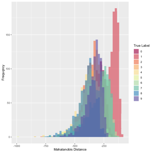
Figure 8: Histograms of the LDA-based Mahalanobis scores using the MNIST data. The data labeled with 0 and 1 are treated as OOD samples in this illustration.

4.3 The Effect of Data Quality and Algorithm

The reliability of AI systems is affected by data quality and the specific algorithms used. The data quality can refer to accuracy in data collection, the efficiency of data collection, the quality of data processing, feature derivation, etc. Take the classification task for illustration, the imbalance and noise in the training set are able to cause the drop of accuracy (ning2019capjack). Here, data imbalance means the imbalance on the proportions of observations among different class labels. Furthermore, the deviation of the distribution of labels in the test set from the training set affects the robustness of AI algorithms as well. It is important to study how data quality affects model accuracy.

Here we give a brief introduction of the method in Lianetal2021Robustness, in which a mixture experimental design was used to study class imbalance in the training set and the difference in distributions of labels from training to test sets. The performance of AI algorithms is measured by the area under the receiver operating characteristic curves, abbreviated by AUC, for each class.

Lianetal2021Robustness provided a framework to study the effect of data quality and algorithms. The XGboost (e.g., chen2015xgboost) and CNN (e.g., kim2014convolutional) are considered. Following the notation from the paper, we define $z_{1}$, which is 1 if the XGboost algorithm is used and is 0 if the CNN algorithm is used. Lianetal2021Robustness investigated the changes on effects of class imbalance generated by two different datasets, the KEGG data, and bone marrow data. The two datasets are derived for the classification of the relationship between gene pairs (YuanBar-Joseph2019). We define $z_{2}$, which is 1 if the KEGG data is used and is 0 if the bone marrow data is used.

A surrogate model established for the performance of AI algorithms, averaged AUC among all classes ($y$), with covariates proportions of labels ($x_{1}$, $x_{2}$, $x_{3}$), AI algorithms ($z_{1}$), and choice of datasets ($z_{2}$) is as following,

$$y =\sum_{j=1}^{m}\beta_{j}x_{j}+\sum_{j<j^{\prime}}\beta_{jj^{\prime}}x_{j}x_{j^{\prime}}+\sum_{k=1}^{h}\sum_{j=1}^{m}\gamma_{kj}z_{k}x_{j}+\sum_{k<k^{\prime}}\delta_{kk^{\prime}}z_{k}z_{k^{\prime}}+\epsilon,$$ (3)

where $m=3$, $h=2$, and $\beta_{j},\beta_{jj^{\prime}}$, $\gamma_{kj}$ and $\delta_{kk^{\prime}}$ are regression coefficients. Note that (3) does not contain a term for main effects of two processing variables $z_{1}$ and $z_{2}$. In order to draw inference for two processing variables, the sum-to-zero constraint is imposed as $\sum_{j=1}^{m}(\gamma_{kj}+\gamma_{k})=0$, where $\gamma_{k}$ is the coefficient for processing variable $z_{k}$.

To maintain the ability of trained AI models identifying classes, the proportions of labels in both training and test sets are at least 0.01. Because of computational constraints, each run has 2 replicates. As shown in Lianetal2021Robustness, Table 2 gives the design of experiments (DOE) for class proportions of the training set with 28 runs.

Table 2: The first 7 runs for the DOE when the covariate factors $z_{1}=1$ (XGboost) and $z_{2}=1$ (KEGG data) are shown in the table. For runs 8-28, the configurations are the cross design of $(x_{1},x_{2},x_{3})$ values in the table with $(z_{1},z_{2})$ taking values in $\{(1,0),(0,1),(1,1)\}$.

Run	$x_{1}$	$x_{2}$	$x_{3}$
1	0.01	0.01	0.98
2	0.01	0.98	0.01
3	0.98	0.01	0.01
4	0.01	0.495	0.495
5	0.495	0.01	0.495
6	0.495	0.495	0.01
7	1/3	1/3	1/3

To explore the effect of deviation in distribution between training set and test set, Lianetal2021Robustness considered three different scenarios, which are balanced scenario, consistent scenario, and reversed scenario. We can see design distinctions among three scenarios. As an illustration, we visualize the results from balanced scenario in which the test set has equal proportion for the three labels. Figure 9 shows the triangle contour plots of prediction for the mean AUC. In general, balanced training datasets produce higher accuracy. For bone marrow data, both algorithms need greater $x_{3}$ to obtain the maximum average AUC. The XGboost outperforms CNN on both datasets. Compared to XGboost, $x_{3}$ has the first priority to CNN as XGboost has a more systematic pattern.

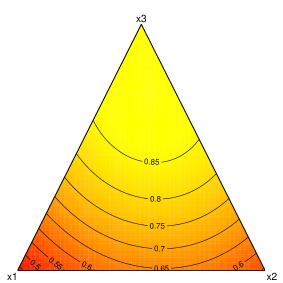
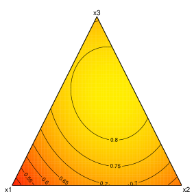
(a) CNN + Bone Marrow	(b) CNN + KEGG
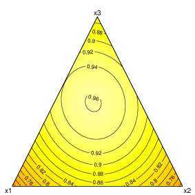
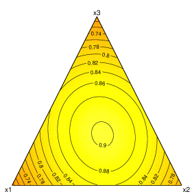
(c) XGboost + Bone Marrow	(d) XGboost + KEGG

Figure 9: Triangle contour plots of the predictions for the mean AUC under four settings: CNN under the bone marrow data (a), CNN under the KEGG data (b), XGboost under the bone marrow data (c), and XGboost under the KEGG data (d).

4.4 Adversarial Attacks

The research on AA focuses on finding adversarial points to the data. Adversarial points $\boldsymbol{x}^{\ast}$ to a given $\boldsymbol{x}$ and the output of the model $f(\boldsymbol{x})$ is defined as the points such that $\|\boldsymbol{x}-\boldsymbol{x}^{\ast}\|$ is small enough for a defined norm (usually $L_{2}$ norm) and $f(\boldsymbol{x})\neq f(\boldsymbol{x}^{\ast})$. To find an adversarial point, one needs to solve the following optimization problem,

$$\min_{\boldsymbol{x}^{\ast}}\|\boldsymbol{x}^{\ast}-\boldsymbol{x}\|\quad\textrm{s.t.}\quad f(\boldsymbol{x}^{\ast})\neq f(\boldsymbol{x}),$$

where $\mathcal{R}$ is some set of perturbations and $\|\cdot\|$ is some norm. Often one can consider $\boldsymbol{x}^{\ast}=\boldsymbol{x}+{\boldsymbol{r}}$ with ${\boldsymbol{r}}$ from a certain set of perturbations.

Adversarial attacks can lead to misclassification, which can further lead to reliability issues. Figure 10 shows an example of AA, in which a horse is recognized as a deer with the added noise. szegedy2013intriguing discovered two counter-intuitive properties of neural networks. One of them is the fact that neural networks can be fooled by in purpose human imperceptible perturbations. After this property of neural networks had been discovered, many researchers were working on why AA is able to easily lead DNN to do misclassification. goodfellow2014explaining used experiments and quantitative results to demonstrate hypotheses about the vulnerability of neural networks. The reason why neural networks are easily fooled by AA is their linear nature and their generalization across structures in order to solve an identical task. goodfellow2014explaining provided a method to generate an adversarial example called fast gradient sign method. There are other AA methods are discovered.

The $L_{q}$ norm is commonly used to measure perturbations between authentic examples and adversarial examples, which is defined as $\|\boldsymbol{x}\|_{q}=\left(\sum_{i=1}^{p}|x_{i}|^{q}\right)^{1/q}$. Here, $p$ is the number of elements of tensor $\boldsymbol{x}=(x_{1},\cdots,x_{p})^{\prime}$. Specifically, the $L_{0}$ norm gives the number of pixels perturbed. The $L_{\infty}$ norm gives the maximum perturbation across all pixels. The $L_{1}$ and $L_{2}$ based AA methods are thoroughly explored, and chen2018ead introduced an AA method based on elastic net regularization combining both $L_{1}$ and $L_{2}$ norms. Not only prediction process of neural networks is vulnerable to AA, ghorbani2019interpretation showed interpretation of neural networks can be drastically twisted without changing the classification results by adversarial perturbations.

chen2019robustness found out that other AI algorithms, such as XGboost, can also suffer from AA. To ensure the accuracy of the AI application, efforts should be made to prevent or mitigate the destruction of AA. From this perspective, it is necessary to detect AA and to study how AA affects the reliability of AI systems.

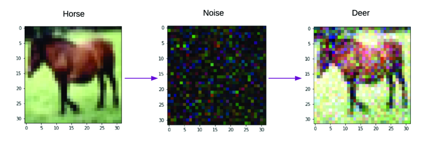
Figure 10: Illustration of adversarial attacks, in which a horse is recognized as a deer with the added noise.

4.5 Model Accuracy and Uncertainty Quantification

An ML/DL model has to be accurate enough (i.e., higher than a threshold) so that the model can be applied in the field. Thus model accuracy is a key factor to reliability. One question that is often asked is how much should trust on the model accuracy, which leads to the uncertainty quantification (UQ) problem. Quantifying the uncertainty of ML models is the key to understand the reliability of model prediction, especially for critical AI tasks.

Much work has been conducted regarding the UQ in DL models. Two types of approaches are often used: the ensemble Monte Carlo approach (abdar2021review) and the Bayesian approach. Ensemble Monte Carlo frameworks usually train multiple models on respective datasets and use models’ predictions as a predictive distribution of the DL model. lakshminarayanan2016simple presented an ensemble method in which a large number of models are trained through re-sampling of the dataset. gal2016dropout proposed the dropout idea to construct multiple models. A random sample of network nodes is dropped out from the model during training. And an empirical distribution over the outputs is built through these multiple models’ predictions.

Bayesian approaches usually assign prior over the network weights and quantify the uncertainty through posterior distribution. Due to the depth and complexity of most DL models, the posterior of Bayesian DL models are often intractable. Thus, the inference based on posterior needs to be done through the Markov Chain Monte Carlo (MCMC) techniques or approximation approaches, such as variational inference (viblei).

However, MCMC sampling methods are usually computationally heavy, while variational inference methods provide efficient alternatives. graves2011practical incorporated variational inference with the Bayesian neural networks (BNN). However, in DL models, the weights often correlated with each other, which leads to the complicated characteristics of the posterior. Simple variational inference may fail to capture the correlation and important characteristics (e.g., multi-mode behavior) of the true posterior. A few efforts have been made to overcome this problem. Different divergence metrics such as $\alpha$-divergence as in hernandez2016black can be used to allow flexible behavior of the variational distribution. Improvements on the variational inference have also been made. miller2017variational used an iterative approach to estimate the mixture component variational distribution. While grover2018variational used the rejection sampling idea to allow the variational distribution approximate to the true posterior.

As an illustration, we describe how variational inference is used to conduct UQ. Consider $n$ observations, and let $\mathcal{X}=\{\boldsymbol{x}_{i}:i=1,\dots,n\}$ be the collection of inputs, where $\boldsymbol{x}_{i}$ is an input tensor. The corresponding response vector is ${\boldsymbol{y}}=\left(y_{1},\dots,y_{n}\right)^{\prime}$. A deep BNN is constructed as $f(\boldsymbol{x},{\boldsymbol{\omega}})$, in which $f(\boldsymbol{x},{\boldsymbol{\omega}})$ denotes the BNN model outputs and ${\boldsymbol{\omega}}$ is a vector that contains all weight parameters in the neural network. The weight parameters ${\boldsymbol{\omega}}$ in the network are treated as random variables.

The response is assumed to follow a normal distribution with the model output as the mean. That is, $(y|\boldsymbol{x},{\boldsymbol{\omega}})\sim\textrm{N}[f(\boldsymbol{x},{\boldsymbol{\omega}}),\sigma^{2}],$ with pdf $f_{\textrm{nor}}[y;f(\boldsymbol{x},{\boldsymbol{\omega}}),\sigma^{2}]$, where $\sigma^{2}$ is the variance. The likelihood function is,

$$p({\boldsymbol{y}}|\mathcal{X},{\boldsymbol{\eta}})=\prod_{i=1}^{n}f_{\textrm{nor}}[y_{i};f(\boldsymbol{x}_{i},{\boldsymbol{\omega}}),\sigma^{2}],$$

where ${\boldsymbol{\eta}}=({\boldsymbol{\omega}}^{\prime},\sigma^{2})^{\prime}$. A prior distribution $p({\boldsymbol{\eta}})$ is assigned over the parameters. By Bayes’ theorem, the posterior of the model parameters is,

$$p({\boldsymbol{\eta}}|\mathcal{X},{\boldsymbol{y}})=\frac{p({\boldsymbol{y}}|\mathcal{X},{\boldsymbol{\eta}})p({\boldsymbol{\eta}})}{\int p({\boldsymbol{y}}|\mathcal{X},{\boldsymbol{\eta}})p({\boldsymbol{\eta}})d{\boldsymbol{\eta}}}.$$

With the posterior distribution, one can make a prediction for a new observation with input $\boldsymbol{x}_{\textrm{new}}$. Specifically, we denote the prediction from the BNN as $y_{\textrm{new}}$. Then the posterior for $y_{\textrm{new}}$ is,

$$p(y_{\textrm{new}}|\boldsymbol{x}_{\textrm{new}},\mathcal{X},{\boldsymbol{y}})=\int f_{\textrm{nor}}[y_{\textrm{new}};f(\boldsymbol{x}_{\textrm{new}},{\boldsymbol{\omega}}),\sigma^{2}]p({\boldsymbol{\eta}}|\mathcal{X},{\boldsymbol{y}})d{\boldsymbol{\eta}}.$$

Due to the high-dimensional parameter space, the exact posterior $p({\boldsymbol{\eta}}|\mathcal{X},{\boldsymbol{y}})$ is usually intractable, so we use a variational distribution $q({\boldsymbol{\eta}};{\boldsymbol{\theta}})$ to approximate it. Here, ${\boldsymbol{\theta}}$ is the parameter vector in the variational distribution. Then the estimate of ${\boldsymbol{\theta}}$ can be obtained by the following optimization,

$${\boldsymbol{\theta}}^{\ast} =\arg\min_{{\boldsymbol{\theta}}}\textrm{KL}[q({\boldsymbol{\eta}};{\boldsymbol{\theta}})\|p({\boldsymbol{\eta}}|\mathcal{X},{\boldsymbol{y}})]$$ (4)

$$=\arg\min_{{\boldsymbol{\theta}}}\left(\mathbb{E}_{q({\boldsymbol{\eta}};{\boldsymbol{\theta}})}\{\log[q({\boldsymbol{\eta}};{\boldsymbol{\theta}})]\}-\mathbb{E}_{q({\boldsymbol{\eta}};{\boldsymbol{\theta}})}\{\log[p({\boldsymbol{y}},{\boldsymbol{\eta}}|\mathcal{X})]\}+\log[p({\boldsymbol{y}}|\mathcal{X})]\right).$$

Here, KL represents the Kullback–Leibler divergence. Because the term $\log[p({\boldsymbol{y}}|\mathcal{X})]$ is constant with respect to ${\boldsymbol{\theta}}$, the optimization in (4) is equivalent to,

$${\boldsymbol{\theta}}^{\ast}=\arg\min_{{\boldsymbol{\theta}}}\left(\mathbb{E}_{q({\boldsymbol{\eta}};{\boldsymbol{\theta}})}\{\log[q({\boldsymbol{\eta}};{\boldsymbol{\theta}})]\}-\mathbb{E}_{q({\boldsymbol{\eta}};{\boldsymbol{\theta}})}\{\log[p({\boldsymbol{y}}|\mathcal{X},{\boldsymbol{\eta}})p({\boldsymbol{\eta}})]\}\right).$$ (5)

The negative of (5) is called the evidence lower bound, and the term $\mathbb{E}_{q({\boldsymbol{\eta}};{\boldsymbol{\theta}})}\{\log[q({\boldsymbol{\eta}};{\boldsymbol{\theta}})]\}$ is the negative entropy of the variational distribution $q({\boldsymbol{\eta}};{\boldsymbol{\theta}})$. The UQ can be carried out based on the estimated variational distribution $q({\boldsymbol{\eta}};{\boldsymbol{\theta}}^{\ast})$.

5 AI Reliability Test Planning

5.1 AI Testing Framework and Test Planning

The key step in AI testing is to build reliability testbeds by using various approaches to collect data on the performance of AI systems or components under various operational and environmental variables. Statistical methods, such as the DOE, computer experiments, and reliability test planning can help with efficient data collection.

For the testing of AI components, most of which are ML/DL algorithms, statisticians can collect data for the performance of algorithms, especially using DOE. For example, a mixture design was used to collect the performance data of AI algorithms as described in Section 4.3. In a traditional setting, in which statisticians are typically participating in the DOE but leave the data collection to the subject experts. However, for AI algorithms, most of them can run with modern computing power, which statisticians have access to. Thus, it provides an opportunity to do the DOE, data collection, and performance data analysis in a streamline.

The testing of AI systems of course is more complicated and most of them have to be run on the field with the hardware and software assembled. Most existing work in test planning for AI systems is in the area of AV driving tests. kalra2016driving used binomial distribution, Poisson distribution and normal approximation to estimate how many miles AVs need to be driven to test they are safe and safer than human drivers. On the other hand, zhao2019assessing indicated the low failure rate is a challenge to obtain the confidence interval and therefore leads to the extreme result in kalra2016driving. Different from kalra2016driving, zhao2019assessing took prior information before road testing and the past data in AV road test into consideration, and used the conservative Bayesian inference framework to calculate how many miles are needed to be driven in AV safety test.

hecker2018failure claimed that how easy the environment is for an AV to drive should also be considered in failure prediction. Although this concept is used only in failure prediction in the paper, it should also be considered in the design of road tests. singh2021simulation proposed a method of generating test-suites and extending old test-suites with new situations based on observations of traffic situations and categorizing situations. hauer2019did raised the question: did all scenarios have been tested? The paper viewed the question as a Coupon Collector’s Problem and proposed a test ending criteria.

Because of the difficulty to run a long way on road, computer simulation can be helpful to test the safety of AVs. Also, the track testing, which is between simulation and real road tests is a good help. fremont2020formal studied the difference results between simulation and track testing. The paper concludes that 62.5% unsafe simulated tests lead to unsafe behavior on track test, and 93.3% safe test leads to safe behavior.

In addition to AVs, another use of the AI product is drones. Delivery drones can be useful in daily lives. According to firstdrone2015, the first Federal Aviation Administration approved drone delivered 24 packages of medicine to rural Virginia. Also, drones can be used in photo captures. Test of safety and reliability of drones is a meaningful topic. However, there are relatively few papers in the test plan of drones. hosseini2017multidisciplinary claimed that the reliability of unmanned aerial vehicle (UAV) should be considered in the designing phase so that it is less likely to redesign the UAV. The paper proposed a design algorithm based on a multidisciplinary optimization method. dawei2014flight pointed out the safety requirements of UAV are different in different flight phases and simulations need to be done in those different flight phases: takeoff, climb, level flight, etc. However, the statistical DOE idea is not well applied in the area of AI system test planning.

5.2 Accelerated Tests

In traditional reliability analysis, accelerated tests (AT) are widely used to obtain information in a timely manner for products that can last for years or even decades. An introduction of AT can be found in EscobarMeeker2006. The basic idea of AT is to test units at high levels of use rate, temperature, voltage, stress, or some other accelerating variables. Based on the data collected on AT, a statistical model is built to predict reliability. AT plays an important role in reliability analysis because it provides an efficient way for rapid product development. Sequential testing idea is also used in reliability test planning (e.g., LeeHongTsengDasgupta2018). AT is also used in software reliability (e.g., Fujiietal2010).

It is natural to think about if the idea of AT can be used in the reliability testing of AI systems, which is mainly applying AT to software testing. The widely used methods for accelerations in the traditional reliability setting are use-rate acceleration, aging acceleration, and stress acceleration. Use-rate acceleration can be applied to software testing by increasing the use cycles. Aging acceleration may not be applicable because software usually does not age. The stress variables used in traditional settings are usually temperature or voltage, which are not applicable for AI testing. However, other types of stress variables can be considered for AI testing.

The failure of software systems is usually use driven. Thus testing under high use rate can speed up the test cycles. It is more likely to observe failure events of AV by driving the AV 200 miles per day instead of driving it 20 miles per day, given all other conditions being comparable. Especially for testing of AI components (i.e., AI algorithms), use-rate acceleration can be easily implemented by running the algorithms at higher use rates.

To increase the stress on the AI systems, one way is to use input-data acceleration. For example, identical twins are a particularly stringent stress test for facial recognition algorithms. Using input data with a lot of noise can test the reliability of the system more easily. In addition, testing the systems under AA can be viewed as a form of input-data acceleration. Operating environment acceleration, which is to test the AI systems under the OOD situation that goes beyond the envelope of the training data, can also put stress on the systems. Also, error injection can be considered as a way of putting stress on the AI algorithms. For example, Bosioetal2019 used fault injections to study the reliability of deep CNN for automotive applications.

In summary, the idea of AT can be applied in AI testing, and additional modeling efforts are needed to make reliability predictions based on the AT data collected over the AI tests. The key step is to model the acceleration factor and link the reliability performance to the normal use condition.

5.3 Improvements for Reliable AI

The ultimate goal of statistical reliability analysis is to improve designs for reliable AI systems. In this section, we discuss several points that can be useful for improvements in AI reliability. Figure 11 shows a flow chart for AI reliability improvement. The following explains the main idea of the flow chart.

As illustrated in Figure 11, starting with an initial design, one can use AT to speed up the development cycles and collect data in a more efficient time manner. Then, one can use statistical modeling to make assessment and prediction for AI reliability, as described in Section 5.2. With failure events observed, one needs to find failure causes. Some of the causes are discussed in Section 2.3. For existing AI failure events, it is important to find the causes of the failures. For example, cause analysis can be applied to those events reported in the AIIncidentDB (2021).

With the cause analysis results, the next step is to do design improvement. The following aspects can be considered: enhancing OOD detection, improving data quality and reducing biases. Enhancing OOD detection is an important component for the overall reliability of the AI systems. It is also crucial to design the operational domain in an appropriate way. We should design algorithms that are more robust to low quality data and are more robust to hardware failures. Meanwhile, it is also important to improve data quality and reduce biases. Choosing algorithms that are more robust to errors can be also important. Architectural vulnerability factor (AVF) is a measure for the vulnerability of the DNN for errors (e.g., Goldsteinetal2020). Using DNN structures that have low AVF can be an effective way to improve the algorithm design for reliable AI.

Iterations can be taken for the four steps (i.e., reliability test, assessment, cause analysis, and improvement) until the reliability reaches the desirable level. Then the system can be deployed to the field. Field tracking is still needed to ensure that the AI system performs the same as it is demonstrated in the development stage.

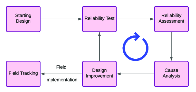
Figure 11: Flow chart for AI reliability improvement.

6 Concluding Remarks

In this paper, we provide statistical perspectives on the reliability analysis of AI systems. The objective of the paper is to provide some general discussion with illustrations on several concrete problems, while we are not trying to be exhaustive in literature review because the AI literature is vast and involves many areas.

We provide a statistical framework and failure analysis for AI reliability. We discuss the traditional reliability methods and software reliability with AI applications. We describe research opportunities including OOD detection, the effect of data quality and algorithms, and model accuracy and UQ with illustrative examples. We also discuss data collection, test planning, and improvements for AI systems. As described in the paper, there are many exciting opportunities in studying the reliability of AI systems and statistics can play an important role in the area.

One challenge is the limited public availability in reliability data from AI systems, which is common for all systems and products because reliability data are usually proprietary and sensitive. Also, the collection of field test data is usually costly and time consuming. The publicly available California DMV database for AV test is one exception. For the reliability data of AI algorithms, as mentioned in Section 5.1, one can collect using in-house computing power. However, it is useful to build data repository for AI reliability datasets. As for modeling methods, Bayesian methods have been widely used in reliability (e.g., Hamadaetal2008). Although we did not discuss Bayesian reliability in this paper, Bayesian methods can be an area that worth exploring for AI reliability modeling.

We would like to remark that this paper focuses on the reliability aspect of AI systems. We do not cover other aspects of AI systems, such as safety, trustworthiness, and security, which also need to be addressed for the large-scale deployment of AI systems. A more broad picture is aiming to address all those issues, called the AI assurance (e.g., batarseh2021survey), of which reliability is certainly an important dimension.

References

- [\citeauthoryearAbdar, Pourpanah, Hussain, Rezazadegan, Liu, Ghavamzadeh, Fieguth, Cao, Khosravi, Acharya, et al.Abdar et al.2021] Abdar, M., F. Pourpanah, S. Hussain, D. Rezazadegan, L. Liu, M. Ghavamzadeh, P. Fieguth, X. Cao, A. Khosravi, U. R. Acharya, et al. (2021). A review of uncertainty quantification in deep learning: Techniques, applications and challenges. Information Fusion 76, 243–297.
- [\citeauthoryearAI IncidentAI Incident] AI Incident. [Online]. Artificial Intelligence Incident Database: https://incidentdatabase.ai, accessed: October 09, 2021.
- [\citeauthoryearAlshemali and KalitaAlshemali and Kalita2020] Alshemali, B. and J. Kalita (2020). Improving the reliability of deep neural networks in NLP: A review. Knowledge-Based Systems 191, 105210.
- [\citeauthoryearAmodei, Olah, Steinhardt, Christiano, Schulman, and ManeAmodei et al.2016] Amodei, D., C. Olah, J. Steinhardt, P. Christiano, J. Schulman, and D. Mane (2016). Concrete problems in AI safety. arXiv: 1606.06565.
- [\citeauthoryearAthavale, Baldovin, Graefe, Paulitsch, and RosalesAthavale et al.2020] Athavale, J., A. Baldovin, R. Graefe, M. Paulitsch, and R. Rosales (2020). AI and reliability trends in safety-critical autonomous systems on ground and air. In 2020 50th Annual IEEE/IFIP International Conference on Dependable Systems and Networks Workshops (DSN-W), pp. 74–77. IEEE.
- [\citeauthoryearBae, Kuo, and KvamBae et al.2007] Bae, S. J., W. Kuo, and P. H. Kvam (2007). Degradation models and implied lifetime distributions. Reliability Engineering and System Safety 92, 601–608.
- [\citeauthoryearBagdonavičius and NikulinBagdonavičius and Nikulin2001] Bagdonavičius, V. and M. S. Nikulin (2001). Estimation in degradation models with explanatory variables. Lifetime Data Analysis 7, 85–103.
- [\citeauthoryearBanerjee, Jha, Cyriac, Kalbarczyk, and IyerBanerjee et al.2018] Banerjee, S. S., S. Jha, J. Cyriac, Z. T. Kalbarczyk, and R. K. Iyer (2018). Hands off the wheel in autonomous vehicles?: A systems perspective on over a million miles of field data. In 2018 48th Annual IEEE/IFIP International Conference on Dependable Systems and Networks (DSN), pp. 586–597. IEEE.
- [\citeauthoryearBaomar and BentleyBaomar and Bentley2016] Baomar, H. and P. J. Bentley (2016). An intelligent autopilot system that learns flight emergency procedures by imitating human pilots. In 2016 IEEE Symposium Series on Computational Intelligence (SSCI), pp. 1–9. IEEE.
- [\citeauthoryearBastani and ChenBastani and Chen1990] Bastani, F. and I.-R. Chen (1990). Assessment of the reliability of AI programs. In Proceedings of the 2nd International IEEE Conference on Tools for Artificial Intelligence, pp. 753–759. IEEE.
- [\citeauthoryearBatarseh, Freeman, and HuangBatarseh et al.2021] Batarseh, F. A., L. Freeman, and C.-H. Huang (2021). A survey on artificial intelligence assurance. Journal of Big Data 8(1), 1–30.
- [\citeauthoryearBlei, Kucukelbir, and McAuliffeBlei et al.2017] Blei, D. M., A. Kucukelbir, and J. D. McAuliffe (2017). Variational inference: A review for statisticians. Journal of the American Statistical Association 112(518), 859–877.
- [\citeauthoryearBlundell, Cornebise, Kavukcuoglu, and WierstraBlundell et al.2015] Blundell, C., J. Cornebise, K. Kavukcuoglu, and D. Wierstra (2015). Weight uncertainty in neural network. In International Conference on Machine Learning, pp. 1613–1622. PMLR.
- [\citeauthoryearBoggs, Wali, and KhattakBoggs et al.2020] Boggs, A. M., B. Wali, and A. J. Khattak (2020). Exploratory analysis of automated vehicle crashes in California: A text analytics & hierarchical Bayesian heterogeneity-based approach. Accident Analysis and Prevention 135, 105354.
- [\citeauthoryearBosio, Bernardi, Ruospo, and SanchezBosio et al.2019] Bosio, A., P. Bernardi, A. Ruospo, and E. Sanchez (2019). A reliability analysis of a deep neural network. In 2019 IEEE Latin American Test Symposium (LATS), pp. 1–6.
- [\citeauthoryearBosnić and KononenkoBosnić and Kononenko2009] Bosnić, Z. and I. Kononenko (2009). An overview of advances in reliability estimation of individual predictions in machine learning. Intelligent Data Analysis 13(2), 385–401.
- [\citeauthoryearCalifornia Department of Motor VehiclesCalifornia Department of Motor Vehicles] California Department of Motor Vehicles. Autonomous vehicle tester program. [Online]. Available: https://www.dmv.ca.gov/portal/vehicle-industry-services/autonomous-vehicles/, accessed: September 01, 2020.
- [\citeauthoryearChen, Zhang, Si, Li, Boning, and HsiehChen et al.2019] Chen, H., H. Zhang, S. Si, Y. Li, D. Boning, and C.-J. Hsieh (2019). Robustness verification of tree-based models. arXiv:1906.03849.
- [\citeauthoryearChen, Sharma, Zhang, Yi, and HsiehChen et al.2018] Chen, P.-Y., Y. Sharma, H. Zhang, J. Yi, and C.-J. Hsieh (2018). EAD: elastic-net attacks to deep neural networks via adversarial examples. In Thirty-second AAAI Conference on Artificial Intelligence, pp. 10–17.
- [\citeauthoryearChen, He, Benesty, Khotilovich, and TangChen et al.2015] Chen, T., T. He, M. Benesty, V. Khotilovich, and Y. Tang (2015). Xgboost: extreme gradient boosting. R package version 0.4-2, 1–4.
- [\citeauthoryearChoi, Jang, and AlemiChoi et al.2018] Choi, H., E. Jang, and A. A. Alemi (2018). WAIC, but why? generative ensembles for robust anomaly detection. arXiv:1810.01392.
- [\citeauthoryearCruiseCruise] Cruise. [Online]. Available: https://www.getcruise.com/, accessed: September 01, 2020.
- [\citeauthoryearDeng and LiDeng and Li2014] Deng, D. and B. Li (2014). Flight safety control and ground test on UAV. In Proceedings of 2014 IEEE Chinese Guidance, Navigation and Control Conference, pp. 388–392. IEEE.
- [\citeauthoryearDengDeng2012] Deng, L. (2012). The MNIST database of handwritten digit images for machine learning research. IEEE Signal Processing Magazine 29, 141–142.
- [\citeauthoryearDixit, Chand, and NairDixit et al.2016] Dixit, V. V., S. Chand, and D. J. Nair (2016). Autonomous vehicles: disengagements, accidents and reaction times. PLoS One 11, e0168054.
- [\citeauthoryearDoherty, Heintz, and KvarnströmDoherty et al.2013] Doherty, P., F. Heintz, and J. Kvarnström (2013). High-level mission specification and planning for collaborative unmanned aircraft systems using delegation. Unmanned Systems 1(01), 75–119.
- [\citeauthoryearEscobar and MeekerEscobar and Meeker2006] Escobar, L. A. and W. Q. Meeker (2006). A review of accelerated test models. Statistical Science 21, 552–577.
- [\citeauthoryearEsteva, Chou, Yeung, Naik, Madani, Mottaghi, Liu, Topol, Dean, and SocherEsteva et al.2021] Esteva, A., K. Chou, S. Yeung, N. Naik, A. Madani, A. Mottaghi, Y. Liu, E. Topol, J. Dean, and R. Socher (2021). Deep learning-enabled medical computer vision. NPJ Digital Medicine 4(1), 1–9.
- [\citeauthoryearFavarò, Eurich, and NaderFavarò et al.2018] Favarò, F., S. Eurich, and N. Nader (2018). Autonomous vehicles disengagements: Trends, triggers, and regulatory limitations. Accident Analysis & Prevention 110, 136–148.
- [\citeauthoryearFremont, Kim, Pant, Seshia, Acharya, Bruso, Wells, Lemke, Lu, and MehtaFremont et al.2020] Fremont, D. J., E. Kim, Y. V. Pant, S. A. Seshia, A. Acharya, X. Bruso, P. Wells, S. Lemke, Q. Lu, and S. Mehta (2020). Formal scenario-based testing of autonomous vehicles: From simulation to the real world. In 2020 IEEE 23rd International Conference on Intelligent Transportation Systems (ITSC), pp. 1–8. IEEE.
- [\citeauthoryearFujii, Dohi, Okamura, and FujiwaraFujii et al.2010] Fujii, T., T. Dohi, H. Okamura, and T. Fujiwara (2010). A software accelerated life testing model. In 2010 IEEE 16th Pacific Rim International Symposium on Dependable Computing, pp. 85–92.
- [\citeauthoryearGal and GhahramaniGal and Ghahramani2016] Gal, Y. and Z. Ghahramani (2016). Dropout as a Bayesian approximation: Representing model uncertainty in deep learning. In International Conference on Machine Learning, pp. 1050–1059. PMLR.
- [\citeauthoryearGhorbani, Abid, and ZouGhorbani et al.2019] Ghorbani, A., A. Abid, and J. Zou (2019). Interpretation of neural networks is fragile. In Proceedings of the AAAI Conference on Artificial Intelligence, Volume 33, pp. 3681–3688.
- [\citeauthoryearGoldstein, Srinivasan, Das, Banerjee, Santiago, Ferreira, Nery, Kundu, and FranaGoldstein et al.2020] Goldstein, B. F., S. Srinivasan, D. Das, K. Banerjee, L. Santiago, V. C. Ferreira, A. S. Nery, S. Kundu, and F. M. G. Frana (2020). Reliability evaluation of compressed deep learning models. In 2020 IEEE 11th Latin American Symposium on Circuits Systems (LASCAS), pp. 1–5.
- [\citeauthoryearGoodfellow, Bengio, and CourvilleGoodfellow et al.2016] Goodfellow, I., Y. Bengio, and A. Courville (2016). Deep Learning. MIT Press.
- [\citeauthoryearGoodfellow, Shlens, and SzegedyGoodfellow et al.2014] Goodfellow, I. J., J. Shlens, and C. Szegedy (2014). Explaining and harnessing adversarial examples. arXiv:1412.6572.
- [\citeauthoryearGravesGraves2011] Graves, A. (2011). Practical variational inference for neural networks. In Advances in Neural Information Processing Systems, pp. 2348–2356. Citeseer.
- [\citeauthoryearGrover, Gummadi, Lazaro-Gredilla, Schuurmans, and ErmonGrover et al.2018] Grover, A., R. Gummadi, M. Lazaro-Gredilla, D. Schuurmans, and S. Ermon (2018). Variational rejection sampling. In International Conference on Artificial Intelligence and Statistics, pp. 823–832. PMLR.
- [\citeauthoryearHamada, Wilson, Reese, and MartzHamada et al.2008] Hamada, M. S., A. Wilson, C. S. Reese, and H. Martz (2008). Bayesian Reliability. New York: Springer.
- [\citeauthoryearHanif, Khalid, Putra, Rehman, and ShafiqueHanif et al.2018] Hanif, M. A., F. Khalid, R. V. W. Putra, S. Rehman, and M. Shafique (2018). Robust machine learning systems: Reliability and security for deep neural networks. In 2018 IEEE 24th International Symposium on On-Line Testing And Robust System Design (IOLTS), pp. 257–260. IEEE.
- [\citeauthoryearHauer, Schmidt, Holzmüller, and PretschnerHauer et al.2019] Hauer, F., T. Schmidt, B. Holzmüller, and A. Pretschner (2019). Did we test all scenarios for automated and autonomous driving systems? In 2019 IEEE Intelligent Transportation Systems Conference (ITSC), pp. 2950–2955. IEEE.
- [\citeauthoryearHecker, Dai, and Van GoolHecker et al.2018] Hecker, S., D. Dai, and L. Van Gool (2018). Failure prediction for autonomous driving. In 2018 IEEE Intelligent Vehicles Symposium (IV), pp. 1792–1799. IEEE.
- [\citeauthoryearHernandez-Lobato, Li, Rowland, Bui, Hernández-Lobato, and TurnerHernandez-Lobato et al.2016] Hernandez-Lobato, J., Y. Li, M. Rowland, T. Bui, D. Hernández-Lobato, and R. Turner (2016). Black-box alpha divergence minimization. In International Conference on Machine Learning, pp. 1511–1520. PMLR.
- [\citeauthoryearHong, Li, and OsbornHong et al.2015] Hong, Y., M. Li, and B. Osborn (2015). System unavailability analysis based on window-observed recurrent event data. Applied Stochastic Models in Business and Industry 31, 122–136.
- [\citeauthoryearHong, Zhang, and MeekerHong et al.2018] Hong, Y., M. Zhang, and W. Q. Meeker (2018). Big data and reliability applications: The complexity dimension. Journal of Quality Technology 50(2), 135–149.
- [\citeauthoryearHosseini, Nosratollahi, and SadatiHosseini et al.2017] Hosseini, M., M. Nosratollahi, and H. Sadati (2017). Multidisciplinary design optimization of UAV under uncertainty. Journal of Aerospace Technology and Management 9, 169–178.
- [\citeauthoryearImran, Posokhova, Qureshi, Masood, Riaz, Ali, John, Hussain, and NabeelImran et al.2020] Imran, A., I. Posokhova, H. N. Qureshi, U. Masood, M. S. Riaz, K. Ali, C. N. John, M. I. Hussain, and M. Nabeel (2020). AI4COVID-19: AI enabled preliminary diagnosis for COVID-19 from cough samples via an app. Informatics in Medicine Unlocked 20, 100378.
- [\citeauthoryearJenihhin, Reorda, Balakrishnan, and AlexandrescuJenihhin et al.2019] Jenihhin, M., M. S. Reorda, A. Balakrishnan, and D. Alexandrescu (2019). Challenges of reliability assessment and enhancement in autonomous systems. In 2019 IEEE International Symposium on Defect and Fault Tolerance in VLSI and Nanotechnology Systems (DFT), pp. 1–6. IEEE.
- [\citeauthoryearJha, Raj, Fernandes, Jha, Jha, Jalaian, Verma, and SwamiJha et al.2019] Jha, S., S. Raj, S. Fernandes, S. K. Jha, S. Jha, B. Jalaian, G. Verma, and A. Swami (2019). Attribution-based confidence metric for deep neural networks. In H. Wallach, H. Larochelle, A. Beygelzimer, F. d’Alché-Buc, E. Fox, and R. Garnett (Eds.), Advances in Neural Information Processing Systems, Volume 32. Curran Associates, Inc.
- [\citeauthoryearKalra and PaddockKalra and Paddock2016] Kalra, N. and S. M. Paddock (2016). Driving to safety: How many miles of driving would it take to demonstrate autonomous vehicle reliability? Transportation Research Part A: Policy and Practice 94, 182–193.
- [\citeauthoryearKaur and BahlKaur and Bahl2014] Kaur, G. and K. Bahl (2014). Software reliability, metrics, reliability improvement using agile process. International Journal of Innovative Science, Engineering & Technology 1(3), 143–147.
- [\citeauthoryearKimKim2014] Kim, Y. (2014). Convolutional neural networks for sentence classification. arXiv:1408.5882.
- [\citeauthoryearKundu, Basu, Sadi, Titirsha, Song, Das, and GuinKundu et al.2021] Kundu, S., K. Basu, M. Sadi, T. Titirsha, S. Song, A. Das, and U. Guin (2021). Special session: Reliability analysis for ML/AI hardware. arXiv:2103.12166.
- [\citeauthoryearLakshminarayanan, Pritzel, and BlundellLakshminarayanan et al.2016] Lakshminarayanan, B., A. Pritzel, and C. Blundell (2016). Simple and scalable predictive uncertainty estimation using deep ensembles. arXiv:1612.01474.
- [\citeauthoryearLambertz, Hartmann, Walsh, Geissler, and McLeodLambertz et al.2014] Lambertz, M., T. Hartmann, S. Walsh, P. Geissler, and D. S. McLeod (2014, 08). Anatomy, histology, and systematic implications of the head ornamentation in the males of four species of Limnonectes (Anura: Dicroglossidae). Zoological Journal of the Linnean Society 172(1), 117–132.
- [\citeauthoryearLawless and CrowderLawless and Crowder2004] Lawless, J. and M. Crowder (2004). Covariates and random effects in a gamma process model with application to degradation and failure. Lifetime Data Analysis 10, 213–227.
- [\citeauthoryearLawlessLawless2003] Lawless, J. F. (2003). Statistical Models and Methods for Lifetime Data (2nd ed.). New Jersey, Hoboken: John Wiley & Sons, Inc.
- [\citeauthoryearLee, Hong, Tseng, and DasguptaLee et al.2018] Lee, I.-C., Y. Hong, S.-T. Tseng, and T. Dasgupta (2018). Sequential Bayesian design for accelerated life tests. Technometrics 60, 472–483.
- [\citeauthoryearLee, Lee, Lee, and ShinLee et al.2017] Lee, K., H. Lee, K. Lee, and J. Shin (2017). Training confidence-calibrated classifiers for detecting out-of-distribution samples. arXiv:1711.09325.
- [\citeauthoryearLee, Lee, Lee, and ShinLee et al.2018] Lee, K., K. Lee, H. Lee, and J. Shin (2018). A simple unified framework for detecting out-of-distribution samples and adversarial attacks. NIPS’18: Proceedings of the 32nd International Conference on Neural Information Processing, 7167–7177.
- [\citeauthoryearLian, Freeman, Hong, and DengLian et al.2021] Lian, J., L. Freeman, Y. Hong, and X. Deng (2021). Robustness with respect to class imbalance in artificial intelligence classification algorithms. Journal of Quality Technology 53, 505–525.
- [\citeauthoryearLiang, Li, and SrikantLiang et al.2017] Liang, S., Y. Li, and R. Srikant (2017). Enhancing the reliability of out-of-distribution image detection in neural networks. arXiv:1706.02690.
- [\citeauthoryearLindqvist, Elvebakk, and HegglandLindqvist et al.2003] Lindqvist, B., G. Elvebakk, and K. Heggland (2003). The trend-renewal process for statistical analysis of repairable systems. Technometrics 45, 31–44.
- [\citeauthoryearLu and MeekerLu and Meeker1993] Lu, C. J. and W. Q. Meeker (1993). Using degradation measures to estimate a time-to-failure distribution. Technometrics 34, 161–174.
- [\citeauthoryearLv, Cao, Zhao, Auger, Sullman, Wang, Dutka, Skrypchuk, and MouzakitisLv et al.2018] Lv, C., D. Cao, Y. Zhao, D. J. Auger, M. Sullman, H. Wang, L. M. Dutka, L. Skrypchuk, and A. Mouzakitis (2018). Analysis of autopilot disengagements occurring during autonomous vehicle testing. IEEE/CAA Journal of Automatica Sinica 5, 58–68.
- [\citeauthoryearMa, Wang, Yang, and YangMa et al.2020] Ma, Y., Z. Wang, H. Yang, and L. Yang (2020). Artificial intelligence applications in the development of autonomous vehicles: a survey. IEEE/CAA Journal of Automatica Sinica 7(2), 315–329.
- [\citeauthoryearMårtensson, Ferreira, Granberg, Cavallin, Oppedal, Padovani, Rektorova, Bonanni, Pardini, Kramberger, Taylor, Hort, Snædal, Kulisevsky, Blanc, Antonini, Mecocci, Vellas, Tsolaki, Kłoszewska, Soininen, Lovestone, Simmons, Aarsland, and WestmanMårtensson et al.2020] Mårtensson, G., D. Ferreira, T. Granberg, L. Cavallin, K. Oppedal, A. Padovani, I. Rektorova, L. Bonanni, M. Pardini, M. G. Kramberger, J.-P. Taylor, J. Hort, J. Snædal, J. Kulisevsky, F. Blanc, A. Antonini, P. Mecocci, B. Vellas, M. Tsolaki, I. Kłoszewska, H. Soininen, S. Lovestone, A. Simmons, D. Aarsland, and E. Westman (2020). The reliability of a deep learning model in clinical out-of-distribution MRI data: A multicohort study. Medical Image Analysis 66, 101714.
- [\citeauthoryearMasunagMasunag2015] Masunag, S. (2015). First FAA-approved drone delivery takes medicine to rural Virginia. https://www.latimes.com/business/la-fi-drone-delivery-20150720-story.html.
- [\citeauthoryearMeeker, Escobar, and PascualMeeker et al.2021] Meeker, W. Q., L. A. Escobar, and F. G. Pascual (2021). Statistical Methods for Reliability Data (Second ed.). New York: John Wiley & Sons, Inc.
- [\citeauthoryearMeeker and HongMeeker and Hong2014] Meeker, W. Q. and Y. Hong (2014). Reliability meets big data: Opportunities and challenges, with discussion. Quality Engineering 26, 102–116.
- [\citeauthoryearMerkelMerkel2018] Merkel, R. (2018). Software reliability growth models predict autonomous vehicle disengagement events. arXiv: 1812.08901.
- [\citeauthoryearMichelmore, Wicker, Laurenti, Cardelli, Gal, and KwiatkowskaMichelmore et al.2019] Michelmore, R., M. Wicker, L. Laurenti, L. Cardelli, Y. Gal, and M. Kwiatkowska (2019). Uncertainty quantification with statistical guarantees in end-to-end autonomous driving control. arXiv: 1909.09884.
- [\citeauthoryearMiller, Foti, and AdamsMiller et al.2017] Miller, A. C., N. J. Foti, and R. P. Adams (2017). Variational boosting: Iteratively refining posterior approximations. In International Conference on Machine Learning, pp. 2420–2429. PMLR.
- [\citeauthoryearMin, Hong, King, and MeekerMin et al.2020] Min, J., Y. Hong, C. B. King, and W. Q. Meeker (2020). Reliability analysis of artificial intelligence systems using recurrent events data from autonomous vehicles. arXiv:2102.01740, 1–30.
- [\citeauthoryearNafreen and FiondellaNafreen and Fiondella2021] Nafreen, M. and L. Fiondella (2021). A family of software reliability models with bathtub-shaped fault detection rate. International Journal of Reliability, Quality and Safety Engineering 28, 2150034.
- [\citeauthoryearNelsonNelson1982] Nelson, W. (1982). Applied Life Data Analysis. New York: John Wiley & Sons.
- [\citeauthoryearNing, Wang, Xin, Li, Zhu, and WuNing et al.2019] Ning, R., C. Wang, C. Xin, J. Li, L. Zhu, and H. Wu (2019). Capjack: capture in-browser crypto-jacking by deep capsule network through behavioral analysis. In IEEE INFOCOM 2019-IEEE Conference on Computer Communications, pp. 1873–1881. IEEE.
- [\citeauthoryearO’Mahony, Campbell, Carvalho, Harapanahalli, Hernandez, Krpalkova, Riordan, and WalshO’Mahony et al.2019] O’Mahony, N., S. Campbell, A. Carvalho, S. Harapanahalli, G. V. Hernandez, L. Krpalkova, D. Riordan, and J. Walsh (2019). Deep learning vs. traditional computer vision. In Science and Information Conference, pp. 128–144. Springer.
- [\citeauthoryearOstrouchov, Maxwell, Ashraf, Engelmann, Shankar, and RogersOstrouchov et al.2020] Ostrouchov, G., D. Maxwell, R. A. Ashraf, C. Engelmann, M. Shankar, and J. H. Rogers (2020). GPU lifetimes on Titan supercomputer: Survival analysis and reliability. In Proceedings of the International Conference for High Performance Computing, Networking, Storage and Analysis (SC’20), New York, NY. Association for Computing Machinery.
- [\citeauthoryearOtter, Medina, and KalitaOtter et al.2020] Otter, D. W., J. R. Medina, and J. K. Kalita (2020). A survey of the usages of deep learning for natural language processing. IEEE Transactions on Neural Networks and Learning Systems 32(2), 604–624.
- [\citeauthoryearPan and YangPan and Yang2009] Pan, S. J. and Q. Yang (2009). A survey on transfer learning. IEEE Transactions on Knowledge and Data Engineering 22(10), 1345–1359.
- [\citeauthoryearPham and PhamPham and Pham2019] Pham, T. and H. Pham (2019). A generalized software reliability model with stochastic fault-detection rate. Annals of Operations Research 277(1), 83–93.
- [\citeauthoryearRajachandrasekar, Besseron, and PandaRajachandrasekar et al.2012] Rajachandrasekar, R., X. Besseron, and D. K. Panda (2012). Monitoring and predicting hardware failures in HPC clusters with FTB-IPMI. In 2012 IEEE 26th International Parallel and Distributed Processing Symposium Workshops & PHD Forum, pp. 1136–1143.
- [\citeauthoryearRamsayRamsay1988] Ramsay, J. O. (1988). Monotone regression splines in action. Statistical Science 3, 425–441.
- [\citeauthoryearSarathy, Baruah, Cook, and WolfSarathy et al.2019] Sarathy, P., S. Baruah, S. Cook, and M. Wolf (2019). Realizing the promise of artificial intelligence for unmanned aircraft systems through behavior bounded assurance. In 2019 IEEE/AIAA 38th Digital Avionics Systems Conference (DASC), pp. 1–8. IEEE.
- [\citeauthoryearSastry and OoreSastry and Oore2020] Sastry, C. S. and S. Oore (2020). Detecting out-of-distribution examples with in-distribution examples and gram matrices.
- [\citeauthoryearSingh, Hari, Tsai, and PitaleSingh et al.2021] Singh, V., S. K. S. Hari, T. Tsai, and M. Pitale (2021). Simulation driven design and test for safety of AI based autonomous vehicles. In Proceedings of the IEEE/CVF Conference on Computer Vision and Pattern Recognition, pp. 122–128.
- [\citeauthoryearSong, Eykholt, Evtimov, Fernandes, Li, Rahmati, Tramèr, Prakash, and KohnoSong et al.2018] Song, D., K. Eykholt, I. Evtimov, E. Fernandes, B. Li, A. Rahmati, F. Tramèr, A. Prakash, and T. Kohno (2018, August). Physical adversarial examples for object detectors. In 12th USENIX Workshop on Offensive Technologies (WOOT 18), Baltimore, MD. USENIX Association.
- [\citeauthoryearSong, Chang, and PhamSong et al.2017] Song, K. Y., I. H. Chang, and H. Pham (2017). A three-parameter fault-detection software reliability model with the uncertainty of operating environments. Journal of Systems Science and Systems Engineering 26(1), 121–132.
- [\citeauthoryearSzegedy, Zaremba, Sutskever, Bruna, Erhan, Goodfellow, and FergusSzegedy et al.2013] Szegedy, C., W. Zaremba, I. Sutskever, J. Bruna, D. Erhan, I. Goodfellow, and R. Fergus (2013). Intriguing properties of neural networks. arXiv:1312.6199.
- [\citeauthoryearWaymoWaymo] Waymo. [Online]. Available: https://waymo.com/, accessed: September 01, 2020.
- [\citeauthoryearWebster and IvanovWebster and Ivanov2020] Webster, C. and S. Ivanov (2020). Robotics, artificial intelligence, and the evolving nature of work. In Digital Transformation in Business and Society, pp. 127–143. Springer.
- [\citeauthoryearWhitmoreWhitmore1995] Whitmore, G. A. (1995). Estimation degradation by a Wiener diffusion process subject to measurement error. Lifetime Data Analysis 1, 307–319.
- [\citeauthoryearWinkens, Bunel, Roy, Stanforth, Natarajan, Ledsam, MacWilliams, Kohli, Karthikesalingam, Kohl, et al.Winkens et al.2020] Winkens, J., R. Bunel, A. G. Roy, R. Stanforth, V. Natarajan, J. R. Ledsam, P. MacWilliams, P. Kohli, A. Karthikesalingam, S. Kohl, et al. (2020). Contrastive training for improved out-of-distribution detection. arXiv:2007.05566.
- [\citeauthoryearWoodWood1996] Wood, A. (1996). Software reliability growth models. Tandem Technical Report 96.1, Tandem Computers, Cupertino, CA.
- [\citeauthoryearYang, Zhang, and HongYang et al.2013] Yang, Q., N. Zhang, and Y. Hong (2013). Statistical reliability analysis of repairable systems with dependent component failures under partially perfect repair assumption. IEEE Transactions on Reliability 62, 490–498.
- [\citeauthoryearYe and ChenYe and Chen2014] Ye, Z.-S. and N. Chen (2014). The inverse Gaussian process as a degradation model. Technometrics 56, 302–311.
- [\citeauthoryearYuan and Bar-JosephYuan and Bar-Joseph2019] Yuan, Y. and Z. Bar-Joseph (2019). Deep learning for inferring gene relationships from single-cell expression data. Proceedings of the National Academy of Sciences 116, 27151–27158.
- [\citeauthoryearZhai and YeZhai and Ye2020] Zhai, Q. and Z.-S. Ye (2020). How reliable should military UAVs be? IISE Transactions 52, 1234–1245.
- [\citeauthoryearZhang, Mukherjee, and LebeckZhang et al.2019] Zhang, X., S. Mukherjee, and A. R. Lebeck (2019). A case for quantifying statistical robustness of specialized probabilistic AI accelerators. arXiv:1910.12346.
- [\citeauthoryearZhao, Banks, Sharp, Robu, Flynn, Fisher, and HuangZhao et al.2020] Zhao, X., A. Banks, J. Sharp, V. Robu, D. Flynn, M. Fisher, and X. Huang (2020). A safety framework for critical systems utilising deep neural networks. arXiv: 2003.05311.
- [\citeauthoryearZhao, Robu, Flynn, Salako, and StriginiZhao et al.2019] Zhao, X., V. Robu, D. Flynn, K. Salako, and L. Strigini (2019). Assessing the safety and reliability of autonomous vehicles from road testing. In 2019 IEEE 30th International Symposium on Software Reliability Engineering (ISSRE), pp. 13–23.
- [\citeauthoryearZhao, Robu, Flynn, Salako, and StriginiZhao et al.2019] Zhao, X., V. Robu, D. Flynn, K. Salako, and L. Strigini (2019). Assessing the safety and reliability of autonomous vehicles from road testing. In 2019 IEEE 30th International Symposium on Software Reliability Engineering (ISSRE), pp. 13–23. IEEE.