Genuine Bistability in Open Quantum Many-Body Systems

Abstract

We analyze the long-time evolution of open quantum many-body systems using a variational approach. For the dissipative Ising model, where mean-field theory predicts a wide region of bistable behavior, we find genuine bistability only at a singular point, confirming the previously suggested picture of a first order transition. The situation is dramatically different when considering a majority-voter model including three-body interactions, where we find bistable behavior in an extended region, owing to the breaking of detailed balance in the the effective description of the system. In this model, genuine bistability persists even when quantum fluctuations are added.

The metaphorically eternal lifetime of thermodynamically unstable diamond gemstones tells us that the minimum free energy is not the only thing that matters when considering the long-time properties of a physical system. Sufficiently large activation barriers can prevent the spontaneous decay of a metastable state even on astronomically large timescales. Here we show that similar behavior can also occur for the steady states of open quantum many-body systems, resolving a long-standing controversy about the existence and limits of bistable behavior in these systems.

In the context of open quantum many-body systems, bistable behavior in the steady state over an extended parameter range is predicted for many different systems by mean-field calculations Lee et al. (2011); Lee and Cross (2012); Marcuzzi et al. (2014); Le Boité et al. (2013); Jin et al. (2013); Le Boité et al. (2014); Mertz et al. (2016); Parmee and Cooper (2018). However, these findings have so far not held up when using more elaborate methods Weimer (2015a, b); Mendoza-Arenas et al. (2016); Maghrebi and Gorshkov (2016); Kshetrimayum et al. (2017); Raghunandan et al. (2018); Jin et al. (2018); Singh and Weimer (2021). This failure of mean-field theory can be partly understood using the variational principle for open systems Weimer (2015a), which allows for the formulation of steady state problems in terms of effective free energy functionals Overbeck et al. (2017). In this setting, one can see that mean-field solutions for open systems do not correspond to the physics above the upper critical dimension, as it is the case for equilibrium problems. However, the question whether other open quantum systems can support true bistability has remained unsolved.

In this Letter, we present a generic framework for describing the long-time evolution of open quantum many-body systems. For this, we establish a Gutzwiller approach for open quantum systems and employ the variational principle for a mapping onto an effective classical problem. In the presence of a dynamical symmtetry Sieberer et al. (2013), fluctuations exhibit thermal statistics, allowing us to employ the statistical theory of metastability Langer (1969). For the dissipative Ising model exhibiting mean-field bistability Lee et al. (2011); Marcuzzi et al. (2014), we demonstrate that the thermodynamically unstable solution eventually decays except around a singular point, confirming the previously suggested picture of a first-order jump in the magnetization Weimer (2015a); Kshetrimayum et al. (2017); Raghunandan et al. (2018). However, the situation is fundamentally different when considering a majority-voter model known as Toom’s model Toom (1980), which has recently found applications in topological quantum error correction Herold et al. (2017); Kubica and Preskill (2019); Vasmer et al. (2021) and the realization of time crystals in open systems Zhuang et al. (2021). For this classical spin model, Monte-Carlo simulations have reported bistable behavior Bennett and Grinstein (1985), which we also observe within our variational approach. We find this behavior being driven by the breaking of detailed balance in the non-equlibirium steady state, which we analyze based on an effective Langevin equation built upon the variational principle. Crucially, we also observe that bistability over an extended region persists under the inclusion of quantum fluctuations in terms of a Hamiltonian driving, constituting the first example of a true bistable phase in an open quantum many-body system.

Gutzwiller theory for open systems.— The Markovian evolution of quantum states in the form of a density matrix $\rho$ can be described by the Liouvillian superoperator $\partial_{t}\rho=\mathcal{L}(\rho)$, in terms of the Lindblad master equation

$$\mathcal{L}(\rho)=-i[H,\rho]+\sum\limits_{j}\Big{[}{c_{j}}^{\dagger}\rho c_{j}-\frac{1}{2}\big{\{}c_{j}^{\dagger}c_{j},\rho\big{\}}\Big{]},$$ (1)

where $H$ is the Hamiltonian of the system and the set of $c_{j}$s represents the jump operators Breuer and Petruccione (2002). This dynamics produces non-equilibrium steady states corresponding to $\mathcal{L}(\rho_{s})=0$. To approximate these states, we consider a Gutzwiller variational ansatz $\rho_{v}=\prod_{i}^{N}\rho_{0}$, where for spin-1/2 particles $\rho_{0}\equiv\Big{(}I+\sum_{\mu\in\{x,y,z\}}\alpha_{\mu}\sigma_{\mu}\Big{)}/2$ is expanded in terms of Pauli matrices $\sigma_{\mu}$, while the corresponding coefficients $\alpha_{\mu}$ are a set of variational parameters. These parameters can be obtained by minimizing a suitable variational cost function. Here, we consider a cost function derived from the vectorized form $\mathopen{\langle\langle}\mathcal{L}^{\dagger}(\rho)\mathclose{|}\mathcal{L}(\rho)\mathclose{\rangle\rangle}$ in terms of the operator inner product $\text{Tr}\{A^{\dagger}B\}=\mathopen{\langle\langle}A^{\dagger}\mathclose{|}B\mathclose{\rangle\rangle}$ inducing the Hilbert-Schmidt norm $||A||_{2}=\sqrt{\text{Tr}\{A^{\dagger}A\}}$. However, as the Hilbert-Schmidt norm is biased towards the maximally mixed state Weimer (2015a), we normalize the cost function by the total purity $\text{Tr}\big{[}\rho^{2}\big{]}=\text{Tr}\big{[}\rho_{0}^{2}\big{]}^{N}$ to counteract the bias Vicentini et al. (2019), i.e. $F_{v}=\mathopen{\langle\langle}\mathcal{L}^{\dagger}(\rho)\mathclose{|}\mathcal{L}(\rho)\mathclose{\rangle\rangle}/\mathopen{\langle\langle}\rho_{0}\mathclose{|}\rho_{0}\mathclose{\rangle\rangle}^{N}$.

For a given (uniform) Liouvillian we can express the square of the Hilbert-Schmidt norm $||A||_{2}^{2}$ as an expansion of its individual terms, geometrical different configurations as it is shown in fig. 1, which in turn can be factorized by some $N$- and $N^{2}$-dependent coefficients. $N$-dependent configurations correspond to those terms in $\mathopen{\langle\langle}\mathcal{L}^{\dagger}(\rho)\mathclose{|}\mathcal{L}(\rho)\mathclose{\rangle\rangle}$ where (fully/partially) mutual lattice sites are acted upon by some elements of $\mathcal{L}^{\dagger}$ and $\mathcal{L}$ while $N^{2}$-dependent configurations represent non-overlapping terms. In addition, these coefficients also encode the lattice dimensionality via their dependency on the coordination number $z$. As a further step to have a scale-independent variational norm, which is required in this study, we treat these coefficients on the same footing, rescaling the $N^{2}$-dependent term to $N$ and then normalize the whole function by $N$. This step can be justified based on the fact that for short-range interacting system the $N$-dependent terms are dominant as they incorporate the overlapping inner products. As a result, the variational norm can be cast into the form

$$f_{v}=\sum\limits_{ij}\frac{\mathopen{\langle\langle}\tilde{\mathcal{L}}_{i}^{\dagger}(\rho)\mathclose{|}\tilde{\mathcal{L}}_{j}(\rho)\mathclose{\rangle\rangle}}{\mathopen{\langle\langle}\rho_{0}\mathclose{|}\rho_{0}\mathclose{\rangle\rangle}^{n_{ij}}},$$ (2)

where $\tilde{\mathcal{L}}_{i}$’s are individual terms in the Liouvillian, similar to what is depicted in fig. 1 and the denominator represents the local purity $\mathopen{\langle\langle}\rho_{0}\mathclose{|}\rho_{0}\mathclose{\rangle\rangle}$ to the power of $n_{ij}$ being the total dimension of the terms in the numerator.

In cases where the coherent and dissipative couplings are uniform, the variational norm can be evaluated analytically for generic Liouvillians even in the thermodynamic limit, analogous to Gutzwiller energies in ground state problems Krauth et al. (1992). This property is in contrast with the more natural trace norm $||A||_{1}=\text{Tr}\{|A|\}$, where additional approximations have to be applied to evaluate the variational norm Weimer (2015a, b).

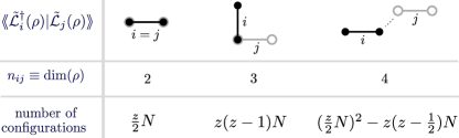
Figure 1: Spatial configurations corresponding to a 2-local Liouvillian appearing on a 2D lattice with the coordination number $z=4$. The black 2-dot lines labelled with $i$ represent $\mathopen{\langle\langle}\tilde{\mathcal{L}}_{i}^{\dagger}(\rho)\mathclose{|}$ and the gray lines labelled with $j$ represent $\mathopen{|}\tilde{\mathcal{L}}_{j}(\rho)\mathclose{\rangle\rangle}$ in the HS norm.

Thermally-activated nucleation processes .— In cases where the variational norm vanishes, the product state solution is an exact steady state of the system. Hence, the value of the variational norm gives direct access to the scale of fluctuations within the system Overbeck et al. (2017). For the first model studied here, these fluctuations obey thermal statistics Sieberer et al. (2013), i.e., they can be captured in terms of an effective temperature $T\sim f_{v}$, considering the fact that the variational norm is also an intensive quantity. Importantly, rewriting the steady state problem of an open quantum many-body systems in terms of a classical statistical mechanics problem allows to employ the vast toolbox for treating the latter. This also applies to the non-equilibrium relaxation dynamics of metastable states Langer (1969). Here, we first compute all local minima of the variational norm. The stability of a local minimim which is not the global one (i.e., a metastable state) can then be quantified in terms of the relaxation rate by which the metastable state relaxes into the global minimum solution.

To calculate the relaxation rate, we consider the path between the metastable minimum and the stable minimum in the variational manifold, which is passing through a saddle-point having a variational norm of $f_{v}^{sp}$. Then, in analogy with the statistical theory of the decay of metastable states Langer (1969), we can express the relaxation rate (per volume) of the metastable solution as

$$I=f_{v}^{sp}\Big{(}\frac{f_{v}^{m}}{2\pi\lambda}\Big{)}^{1/2}e^{-\tilde{E}_{a}/f_{v}^{m}},$$ (3)

where $f_{v}^{m}$ is the value of variational norm of the metastable state and $\lambda$ is the curvature of a saddle-point in the activation energy, see below. The equivalent of the activation energy $\tilde{E}_{a}$ is given here by the variational cost of a critical nucleus of the stable solution (created by random fluctuations) within a system in the metastable state. In the following, we estimate $\tilde{E}_{a}$ based on classical nucleation theory Chaikin and Lubensky (1995). By considering square-shaped nucleus with the length $\ell$, we obtain

$$E_{a}=-\ell^{2}(f_{v}^{m}-f_{v}^{s})+4\ell(f_{v}^{sp}-f_{v}^{m}),$$ (4)

which respectively consists of a volume energy of the nucleus, with $f_{v}^{s}$ being the value of variational norm of the stable state, and a surface tension of its domain wall Chaikin and Lubensky (1995). $\tilde{E}_{a}$ is then defined as the maximized activation energy with the critical length $\ell^{\ast}=2(f_{v}^{sp}-f_{v}^{m})/(f_{v}^{m}-f_{v}^{s})$. Concerning the surface tension, we consider a localized sharp kink, in the order of the lattice spacing, separating the stable nucleus from the rest. We have numerically verified that employing a smooth kink using an additional gradient term does not result in any significant change. Finally, $\lambda=2(f_{v}^{m}-f_{v}^{s})>0$ is defined as the second derivative of $E_{a}$ with respect to $\ell$ Langer (1969).

a

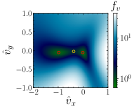
b

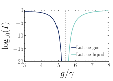
Figure 2: (a) Variational norm $f_{v}$ of the dissipative Ising model at the first-order transition ($J/\gamma=5,g/\gamma=5.40\pm 0.01$) in a plane of transformed variational parameters $\hat{v}_{x}(\alpha_{x,y,z})$ and $\hat{v}_{y}(\alpha_{x,y,z})$ spanned by the two minima (red circles) and the intermediate saddle-point (yellow circle). The left and right minima correspond to the gas and liquid phase, respectively. (b) Logarithm of the relaxation rate $\log_{10}(I)$ of the metastable solution as a function of $g/\gamma$, showing a steep dip close to the phase transition.

Dissipative Ising model.— As the first concrete model, we turn to the paradigmatic dissipative Ising model, as it is a widely studied model, where mean-field bistability gives way to a first-order transition. Its Hamiltonian part is given by

$$H=\frac{g}{2}\sum\limits_{i}\sigma_{x}^{(i)}+\frac{J}{4}\sum\limits_{\langle ij\rangle}\sigma_{z}^{(i)}\sigma_{z}^{(j)},$$ (5)

where $g$ and $J$ indicate the strength of the transverse field and of the Ising interaction, respectively. Dissipation is incorporated by adding spin flips in the form of quantum jump operators $c_{i}=\sqrt{\gamma}\sigma_{-}^{(i)}$ with the rate $\gamma$.

Within our variational approach, we can obtain approximative steady-state solutions by minimizing the variational norm $f_{v}$ of Eq. (2). Close to the transition, our variational results show a double basin structure, see Fig. 2, indicating the presence of two competing phases (i.e., liquid and gas), separated by a saddle point. We note that our results for the position of the first-order transition are in excellent agreement with other calculations Weimer (2015a, b); Kshetrimayum et al. (2017); Jin et al. (2018); Singh and Weimer (2021). Crucially, the value of the variational norm at the two minima is different except exactly at the first-order transition. To analyze the fate of the metastable state (i.e., the local minimum with the higher variational norm), we compute the relaxation rate defined in eq. (3) to quantitatively assess long-time stability of the metastable solution. As shown in fig. 2b, the rate is finite far away from the transition and the metastable solution quickly relaxes into the stable one. However, for a narrow width of $g/\gamma$, the relaxation rate of the metastable state drastically decreases, explaining the experimentally observed hysteresis close to the transition Carr et al. (2013). However, this long-lasting metastability is not a genuine thermodynamic phase, as the relaxation rate is an analytic function over the entire parameter range.

Toom’s majority voting model.— To answer the question whether it is possible to observe genuine bistability in an open quantum system, we turn to Toom’s majority voting model, which supports bistabiliy in a classic non-equilbrium setting Toom (1980); Bennett and Grinstein (1985); Gćcs and Reif (1988); Grinstein (2004). This model has recently found renewed interest because of its relevance for topological quantum error correction Herold et al. (2017); Kubica and Preskill (2019); Vasmer et al. (2021) and time crystals in open systems Zhuang et al. (2021). We explain how genuine bistability arises in Toom’s model within our variational framework and show that this bistability is robust under the addition of quantum fluctuations. Toom’s model is a set of classical rate equations for a system of binary variables (i.e., 0 and 1), which can be cast into a fully dissipative (i.e., $H=0$) Lindblad master equation, governed by the jump operators

$$c_{j,\mu}=\sqrt{\gamma_{\mu}}\sigma_{-}^{j}M_{0}^{(j,j+E,j+N)}$$ (6)

$$c_{j,\bar{\mu}}=\sqrt{\bar{\gamma}_{\mu}}\sigma_{+}^{j}M_{0}^{(j,j+E,j+N)}$$ (7)

$$c_{j,\nu}=\sqrt{\gamma_{\nu}}\sigma_{+}^{j}M_{1}^{(j,j+E,j+N)}$$ (8)

$$c_{j,\bar{\nu}}=\sqrt{\bar{\gamma}_{\nu}}\sigma_{-}^{j}M_{1}^{(j,j+E,j+N)}$$ (9)

where $\sigma_{-}=\mathopen{|}0\mathclose{\rangle}\mathopen{\langle}1\mathclose{|}$ and $\sigma_{+}=\mathopen{|}1\mathclose{\rangle}\mathopen{\langle}0\mathclose{|}$ are the lowering and raising operators, respectively, acting on the site $j$ on a square lattice, depending on the state of $j$ and its northern and eastern neighbors, expressed in terms of the majority vote operators $M_{s}$. Here, $M_{0}$ and $M_{1}$ refer to the configurations of the three sites where the majority is in the 0 and 1 state, respectively, see Tab. 1 for all possible configurations. Importantly, rates with index $\mu$ and $\nu$ refer to lowering and raising operations, respectively, while barred and unbarred rates are operations against and with the majority, respectively.

NCE state	101	111	110	011	010	100	001	000
Operation	$\sigma_{+}$	$\sigma_{-}$	$\sigma_{-}$	$\sigma_{-}$	$\sigma_{-}$	$\sigma_{+}$	$\sigma_{+}$	$\sigma_{+}$
rate	$\gamma_{\nu}$	$\bar{\gamma}_{\nu}$	$\bar{\gamma}_{\nu}$	$\bar{\gamma}_{\nu}$	$\gamma_{\mu}$	$\bar{\gamma}_{\mu}$	$\bar{\gamma}_{\mu}$	$\bar{\gamma}_{\mu}$

Table 1: Ruleset and the corresponding transition rates for Toom’s model indicating how the central site is updated according to the North-Center-East (NCE) state.

While the deterministic limit of Toom’s model, i.e. $\bar{\gamma}_{\mu}=\bar{\gamma}_{\nu}=0$ can readily eliminate minority islands, Toom has rigorously proved that this ability persists even in the presence of updates against the majority rule, provided that the probability of such events is sufficiently low Toom (1980); Lebowitz et al. (1990). This makes Toom’s model a fault-tolerant error correcting model for a finite range of the noise Kubica and Preskill (2019). Although Toom’s original proof is only relevant to the case where the sites are updated synchronously, it has been shown that the argument also holds for simultaneous updates in a master equation formalism Gray (1999).

Using a global evolution rate $\gamma$, Toom’s model can be characterized in a dimensionless two-parameter space of noise and bias, according to the noise amplitude $T=e^{-\gamma_{\nu}/\gamma}+e^{-\gamma_{\mu}/\gamma}$, analogous to temperature, and with bias $h=(e^{-\gamma_{\nu}/\gamma}-e^{-\gamma_{\mu}/\gamma})/T$, analogous to a symmetry-breaking external magnetic field in the Ising model. In the case of unbiased noise $h=0$, the model behaves like the zero-field Ising model with a continuous transition at a critical temperature. However, even at the presence of biased noise the model undergoes a first-order transition between a bistable phase and a unique ergodic phase. This behavior arises from the chirality of the jump operators in Eq. (9), as they do not contain the west and south sites He et al. (1990); Muñoz et al. (2005). Basically, any chiral updating rule leads to a violation of the detailed balance condition, which is necessary when trying to obtain a stationary state that does not exhibit thermal statistics Grinstein (2004).

In the presence of thermal statistics, it is relatively straightforward to express the variatonal norm of Eq. (2) in terms of a Ginzburg-Landau-Wilson framework and then apply standard techniques for the study of critical phenomena such as a perturbative renormalization group treatment Overbeck et al. (2017) to obtain the steady-state phase diagram. However, we cannot take this route here as the lack of detailed balance can lead to non-thermal steady states. To overcome this obstacle, we introduce a Langevin equation to describe the full relaxation dynamics of the observables $\phi_{i}=\langle\sigma_{z}^{(i)}\rangle$. To this end, we first perform a gradient expansion of the variational norm, i.e., $f_{v}(\{\phi_{i}\})=\sum_{i}f_{i}(\phi_{i},\nabla\phi_{i})$, where $\nabla\phi_{i}=(\phi_{i+E}-\phi_{i},\phi_{i+N}-\phi_{i})$ is the lattice gradient . The Langevin equation is then given by $\partial_{t}\phi_{i}=-\partial f_{v}/\partial\phi_{i}+\xi_{i}$, yielding

$$\frac{\partial}{\partial t}\phi_{i}=-\Big{[}\frac{\partial f_{0}}{\partial\phi_{i}}-a-(b-b^{\prime})\nabla\phi_{i}-2b^{\prime}\phi_{i}-c\nabla^{2}\phi_{i}\Big{]}+\xi_{i},$$ (10)

where $f_{0}$ denotes the variational norm for the homogenous case without any gradient terms and $\xi_{i}$ is a white Gaussian noise, i.e. $\langle\xi_{i}\rangle=0$ and $\langle\xi_{i}(t)\xi_{j}(0)\rangle=f_{0}^{m}\delta_{i,j}\delta(t)$ with $f_{0}^{m}$ (the variational norm of the metastable solution) as the effective temperature Note (1). Furthermore, we have truncated the gradient expansion at second order. Our Langevin equation differs from that of conventional kinetic Ising models Hohenberg and Halperin (1977) due to the appearance of a linear gradient term with coefficient $(b-b^{\prime})>0$ which captures the chirality of the jump operators. Here, a sufficiently large $(b-b^{\prime})$ ensures the shrinkage of minority islands of either states. Importantly, similar Langevin equations for the Toom’s model have already been proposed on a purely phenomenological level He et al. (1990), while in our variational approach, all coupling constants can be directly calculated from the microscopic model. We also note that our Langevin equation is on equal footing to those that can be derived within the Keldysh formalism Sieberer et al. (2016), however, performing such calculations for spin systems is often challenging because of the hard-core constraint imposed by spins Kiselev and Oppermann (2000).

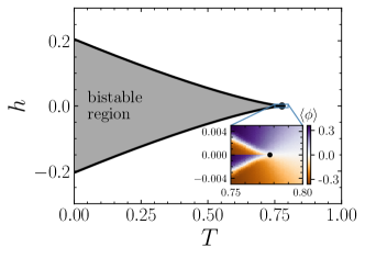
Figure 3: Phase diagram of The Toom’s model shows two phase transition lines separating a bistable phase (gray) from an ergodic phase (white), meeting at a critical point at $T_{c}=0.777\pm 0.001$ (black dot). The inset shows how the orientation of stationary magnetization (starting from a majority of sites polarized against the bias) changes in different zones close to criticality.

We are now in the position to calculate the phase diagram of Toom’s model in the $T-h$ plane by solving the Langevin equation for a $20\times 20$ lattice and averaging over 100 samples initialized in a configuration polarized against the bias field Note (1). Fig. 3 demonstrates an extended region of bistability in the absense of the $Z_{2}$ symmetry of the Ising model that has no counterpart in the corresponding equilibrium system. We note that due to the asynchronicity of master equation in contrast to the Toom’s original updating rules, the phase diagram quantitatively differs from that of the synchronous model Bennett and Grinstein (1985), but the qualitative behavior is identical. According to the numerical simulation close to criticality, two lines separate the bistable region from the ergodic one ending up to an Ising critical point at $T_{c}=0.777\pm 0.001$ on the $h=0$ line, as shown in the inset of Fig. 3.

a

b

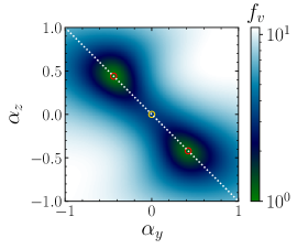
c

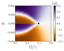
Figure 4: Bistability in the variational steady state of Toom’s model in the presence of quantum fluctuation. Variational norm (in logarithmic scale) is depicted as a function of $\alpha_{z}$ and $\alpha_{y}$ for $H=T=0.15$ deep in (a) the bistable phase with $\Omega/\gamma=0.15$ and (b) the ergodic phase with $\Omega/\gamma=2.0$. The dotted lines show the axis of the effective classical field. (c) Phase diagram in the presence of quantum fluctuations at $T=0.75$ showing gradual shrinkage of the bistable region by increasing $\Omega$ ending up with a critical point (black square) at $\Omega_{c}/\gamma=0.39\pm 0.02$ similar to the classical case.

Having shown that our variational approach is able to reproduce the phase diagram of the classical model, we now turn to the addition of quantum fluctuations. In the context of Toom’s model, this can be done in a natural way in terms of a PXP Hamiltonian of the form

$$H=\Omega\sum_{j}\big{[}P_{0}^{(j+N)}\sigma_{x}^{(j)}P_{0}^{(j+E)}+P_{1}^{(j+N)}\sigma_{x}^{(j)}P_{1}^{(j+E)}\big{]},$$ (11)

where $P_{i}=\mathopen{|}i\mathclose{\rangle}\mathopen{\langle}i\mathclose{|}$ is a projection operator acting on the northern and eastern neighbors. Such PXP terms are of great interest in the investigation of strongly interacting Rydberg systems Sun and Robicheaux (2008); Turner et al. (2018); Bluvstein et al. (2021), while the realization of the jump operators of Eq. (9) is also feasible within these systems Wintermantel et al. (2020). In the language of Toom’s model, these quantum fluctuations act against the local majority and therefore provide a new source of quantum noise to the update rules. Additionally, the Hamiltonian conserves $\sigma_{x}$ on all sites, hence the variational Gutzwiller ansatz can be parameterized using only $\alpha_{y}$ and $\alpha_{z}$. We first perform a rotation of the variational parameters according to $\phi=\cos(\theta)\alpha_{z}+\sin(\theta)\alpha_{y}$ with $\theta=\arctan(\alpha_{y}/\alpha_{z})$. Importantly, this rotation results in $\phi$ containing all the critical behavior of the system, while the ortogonal field $\phi_{\perp}$ can be approximated by a quadratic term close to the variational mimima, see Fig. 4, i.e., it is always gapped. Importantly, while quantum fluctuations lead to a renormalization of the coupling constants of the Langevin equation for $\phi$, its form remains unchanged.

To obtain the phase diagram in the presence of quantum fluctuations, we first compute the homogeneous variational norm $f_{v}$ in terms of $\alpha_{y}$ and $\alpha_{z}$. Figs. 4a and 4b show the variational landscape deep in the bistable phase and the ergodic phase, respectively. We then compute the phase diagram in the $\Omega-h$ plane close to the Ising critical point at $T=0.75$, see Fig. 4c. Crucially, we find extended bistability even in the presence of quantum fluctuations. Essentially, deep in the bistable region (Fig. 4a), small amounts of quantum fluctuations cannot overcome the bistability barrier because the strength of the fluctuations indicated by the variational norm $f_{v}$ is very small. However, by increasing $\Omega$ (Fig. 4b), both the strength of the fluctuation increases substantially and the barrier separating the two variational minima is greatly decreased, leading to ergodic behavior. Finally, similar to the classical case, the phase boundaries separating the bistable from the ergodic phase meet in a critical point on the $Z_{2}$-symmetric line given by $h=0$. We have also investigated the phase diagram for different Hamiltonian perturbations such as a transverse field proportional to $\sigma_{x}$, where we find qualitatively similar behavior. This suggests that Toom’s model can serve as an error-correcting code in the presence of generic quantum fluctuations.

To summarize, we have developed a method for assessing the long-time evolution of open many-body systems. In the presence of a dynamical symmetry giving rise to thermal statistics of the steady state, one can calculate the relaxation rate using a statistical approach built on classical nucleation theory. In the absence of the dynamical symmetry, we find that the time evolution of the system can be captured in terms of an effective Langevin equation, which allows to map out the steady-state phase diagram of systems violating detailed balance, where we find the first instance of genuine bistability in an open quantum system when adding quantum fluctuations to Toom’s majority voting model. Our approach can be used for many other critical systems that are otherwise inherently difficult to treat, such as quantum contact processes Carollo et al. (2019), systems exhibiting limit cycles Owen et al. (2018), or neural networks based on open quantum systems Rotondo et al. (2018).