Universality (beyond leading log) of soft radiative corrections to $\hat{q}$ in $p_{\perp}$ broadening and energy loss

Abstract

It has been known for many years that soft radiation can give potentially large double-logarithm corrections to $p_{\perp}$ broadening of a high-energy particle traveling through QCD matter, but that this soft radiation correction can be absorbed into an effective value $\hat{q}_{\rm eff}$ for the medium $p_{\perp}$-broadening parameter $\hat{q}$. Here “soft” means high energy compared to medium scales but soft compared to the original high-energy particle traveling through the medium. A similar situation arises in the case of soft corrections to hard splitting of a high-energy particle, such as hard $g{\to}gg$, where double logarithms can also be absorbed using the same effective $\hat{q}_{\rm eff}$. In this paper, I study whether the same holds true for potentially large, subleading, single-logarthim corrections. The correspondence is more indirect for single logarithms, but I show (in the large-$N_{\rm c}$ limit) that single logarithms from soft radiation in the case of $p_{\perp}$ broadening also determine the single logarithms from soft radiative corrections to hard $g{\to}gg$ splitting. Along the way, there is an interesting variation of the original BDMPS-Z calculation of splitting rates in the $\hat{q}$ approximation. I also discuss how, for soft-radiative corrections to hard splitting processes, there are two different types of “$\hat{q}_{\rm eff}$” that come into play, which differ by “$i\pi$” terms that multiply single logarithms.

1 Introduction

High-energy partons traveling through hot or cold QCD matter receive random transverse momentum kicks from multiple small-angle scattering with the medium. The typical total transverse momentum change $p_{\perp}$ after traveling through a length $L$ of medium involving many such interactions is parametrized as

$$\langle p_{\perp}^{2}\rangle=\hat{q}L,$$ (1)

where $\hat{q}$ is determined by characteristics of the medium. $\hat{q}$ also appears in formulas for high-energy parton splitting rates in the medium. For example, formalism developed by Baier, Dokshitzer, Mueller, Peigné, and Schiff BDMPS1 ; BDMPS2 ; BDMPS3 ; BDMS and Zakharov Zakharov1 ; Zakharov2 ; Zakharov3 (BDMPS-Z) gives (in appropriate limits) the in-medium gluon splitting rate

$$\frac{d\Gamma}{dx}=\frac{\alpha_{\rm s}P_{g\to gg}(x)}{2\pi}\sqrt{\frac{(1{-}x{+}x^{2})\hat{q}_{\rm A}}{x(1{-}x)E}}$$ (2)

for $g\to gg$ with energies $E\to xE,(1{-}x)E$. (The subscript of $\hat{q}_{\rm A}$ indicates the $\hat{q}$ appropriate for the adjoint color representation, i.e. for gluons, and $C_{\rm A}{=}N_{\rm c}$ is the adjoint-representation quadratic Casimir.)

In the original picture (fig. 1a) of momentum broadening motivating (1), $\hat{q}$ is determined by small-angle elastic scattering rates of high-energy particles scattering from the medium. Liou, Mueller, and Wu (LMW) LMW realized that soft gluon radiation accompanying elastic scatterings (fig. 1b) can also carry away transverse momentum and so change $p_{\perp}$ in an important way. Formally, this effect is suppressed by a power of $\alpha_{\rm s}$ but is enhanced by what can be a potentially large double logarithm. They found that such logarithms could be absorbed into an effective value $\hat{q}_{\rm eff}=\hat{q}+\delta q$ of $\hat{q}$. To leading-log order, the soft radiation effects are accounted for by

$$\delta\hat{q}=\frac{C_{\rm A}\alpha_{\rm s}}{2\pi}\ln^{2}\Bigl{(}\frac{L}{\tau_{0}}\Bigr{)}\,\hat{q},$$ (3)

where $\tau_{0}$ is the scale of the mean-free path for typical small-angle elastic scattering in the medium. They also worked out how to resum the effects of multiple soft gluon bremsstrahlung to leading-log order. Later, various authors Blaizot ; Iancu ; Wu investigated similar effects for in-medium splitting rates such as (2). That is, what would be the effect on $q\to qg$ or $g\to gg$ (fig. 2a) of having an additional softer bremsstrahlung (fig. 2b) occur during an underlying, harder in-medium splitting process. They again found a double logarithm. Moreover, they found that the effect was completely accounted for, at leading-log order, simply by making the same modification (3) to the $\hat{q}$ appearing in splitting rates such as (2). So, there are important soft radiative corrections, but they are universal in that they can be absorbed into $\hat{q}$ in a way that is independent of whether your interest is $p_{\perp}$ broadening or splitting rates.

Figure 1: (a) A cartoon of transverse momentum broadening as a high-energy particle traverses a QCD medium. The arrows represent small transverse momentum kicks from the medium due to small-angle elastic scattering with the medium. (b) The same, but here some transverse momentum is also carried away by a relatively soft (but still high-energy) bremsstrahlung.

Figure 2: (a) A hard, underlying splitting process (bremsstrahlung or pair production) with energies $E\to xE,(1{-}x)E$. (b) One example of adding an additional, softer gluon bremsstrahlung, which should be understood as occurring during the formation time of the underlying, harder splitting process (a).

In the context of $p_{\perp}$ broadening, LMW also computed the single-log correction, sub-leading to the double-log correction (3). In this paper, I examine whether the single-log correction is also universal. At first sight, it may not seem to be. Ref. logs recently extracted, in the large-$N_{\rm c}$ limit, the soft single-log corrections to the hard splitting rate (2) from more-general results for $g\to ggg$ (e.g. fig. 2b with nothing soft). As I will review, the coefficient of that single log is a slightly complicated function of the energy fraction $x$ of the daughter of the hard splitting process (fig. 2a), which has no analog in the discussion of $p_{\perp}$ broadening (fig. 1a). Nonetheless, we will see that there is a connection. I will show that the slightly complicated soft single-log correction to hard splitting can be exactly reproduced from the simpler LMW result for the soft single-log correction to $p_{\perp}$ broadening. We will see that this requires re-doing the BDMPS-Z calculation of (2) in a more general way that allows incorporation of the LMW result.

That calculation will verify, in a highly non-trivial example, that the soft single-log corrections to $\hat{q}$ are universal (and that they completely account for all soft single-log corrections to hard splitting). This will also be an important cross-check of the more general calculation of the non-soft overlapping splitting $g\to gg\to ggg$ in refs. 2brem ; seq ; dimreg ; QEDnf ; qcd .

It would be nice to also have a relation between the single logs that is not embedded in the cogs of a re-derivation of the BDMP-Z formula. Inspired by that equivalence, I later find a way to algebraically rewrite the formula for the previously known single-log correction logs to hard splitting in ways that more directly connect to the LMW result for $p_{\perp}$ broadening. That version will be a re-writing, not a re-derivation, of the single logs. But it will isolate more clearly the physics of the single log result and may be useful in applications.

Outline

In the next section, I review the phase space for soft emission that gives rise to double logarithms, and I give some important caveats about exactly what will be checked in this paper regarding single logarithms. In section 3, I then quote the already-known results for single logarithms from soft radiative corrections to $p_{\perp}$ broadening and to hard $g{\to}gg$ splitting. I also give a short, qualitative review of the formalism underlying LMW’s calculation for $p_{\perp}$ broadening and explain why one cannot instantly apply their $\hat{q}_{\rm eff}$ result to the usual rate formula for hard $g{\to}gg$ splitting. Section 4 briefly reviews the BDMPS-Z based derivation of the hard splitting rate (2) as preparation for modifying that derivation in section 5 to properly incorporate the $\hat{q}_{\rm eff}$ from $p_{\perp}$ broadening. Section 5 will successfully reproduce the single logarithm previously extracted in ref. logs , but using here a much simpler calculation that assumes universality of soft radiative corrections to $\hat{q}$. We will also see that, at the level of soft radiative corrections, there is a difference between a $\hat{q}_{\rm eff}$ involving (i) one particle in the amplitude and one in the complex conjugate amplitude vs. (ii) two particles in the amplitude. One gets both types of $\hat{q}$’s appearing in splitting calculations; to my knowledge, a difference between (i) and (ii) in this context has not previously been demonstrated. In section 6, I show a variety of ways of writing the final result for soft corrections to hard $g{\to}gg$ splitting in terms of the result for $\hat{q}_{\rm eff}$ from $p_{\perp}$ broadening, along with some qualitative explanation of the results. The most compact formulation is presented in section 7, where I give my conclusions.

2 Caveats and Assumptions

2.1 The double log region

Throughout this paper, I will draw diagrams for contributions to splitting rates using the conventions of ref. 2brem , which are adapted from Zakharov’s description of splitting rates Zakharov1 ; Zakharov2 ; Zakharov3 . In fig. 3a, the blue factor represents the calculation of the splitting amplitude in (lightcone) time-ordered perturbation theory. The red factor is the conjugate amplitude. Fig. 3b shows the same time-ordered contribution to the rate, depicted by sewing together the amplitude and conjugate amplitude. I then follow Zakharov’s picture of re-interpreting the right-hand diagrams as three particles propagating forward in time. Only the high-energy particle lines are shown in these diagrams: the lines implicitly interact with the medium as they propagate, and there is an implicit average of the rate over the randomness of the medium.

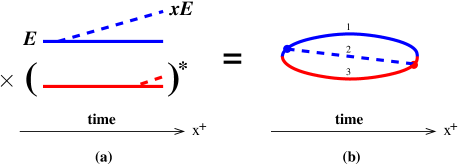
Figure 3: (a) A time-ordered contribution to the rate for single splitting, such as $g\to gg$ of high-energy gluons, with amplitude in blue and conjugate amplitude in red. (b) A single diagram representing this contribution to the rate. In both cases, all lines implicitly interact with the medium. We need not follow particles after the emission has occurred in both the amplitude and conjugate amplitude because I will consider only the $p_{\perp}$-integrated rate. (See, for example, section 4.1 of ref. 2brem for a more explicit argument, although applied there to a more complicated diagram.) Nor need we follow them before the first emission because we approximate the initial particle as on-shell. Only one of the two time orderings that contribute to the rate is shown above.

Fig. 4 depicts a soft radiative correction (the magenta line) to the underlying splitting process of fig. 3b. Throughout this paper, I will refer to the energy of the initial high-energy particle in the underlying hard splitting process as $E$ and to the energy of the soft radiative gluon as

$$\omega_{y}\equiv yE,$$ (4)

as in fig. 2. As shown in fig. 4, I define $\Delta t_{y}$ to be the separation between times of the $y$ emissions in the amplitude and conjugate amplitude, which is to be integrated over.

For the underlying hard splitting process $E\to xE,(1{-}x)E$, it will be convenient for qualitative, parametric discussions to take $xE$ to be the smaller of the two daughters. The eventual derivations and results, however, will be symmetric with respect to $x{\to}1{-}x$. I will not assume $x\ll 1$ (though that case is also covered by the analysis provided $y\ll x$). It’s sometimes convenient to also write the $x$ daughter energy as $\omega_{x}$:

$$\omega_{x}\equiv xE.$$ (5)

In my analysis, “soft” $y$ means soft compared to $x$ but still high-energy compared to medium scales:

$$\mbox{(medium scale)}\ll\omega_{y}\ll\omega_{x}.$$ (6)

(For a quark-gluon plasma, “medium scale” above just means the temperature $T$.) Parametrically, I will refer to the typical duration of the splitting process as the $x$ formation time

$$t_{\rm form}(x)\sim\sqrt{\frac{\omega_{x}\vphantom{E}}{\hat{q}}}=\sqrt{\frac{xE}{\hat{q}}}\,.$$ (7)

Here and throughout, I will study the simple case where the medium is homogeneous over the formation time (and corresponding length).

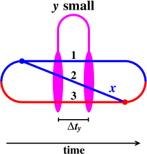
Figure 4: The rate diagrams which (together with their complex conjugates) produce the double logarithm Iancu ; Blaizot ; Wu . On each end, the relatively-soft $y$ gluon may connect to any of the three lines of the underlying splitting process. In my analysis, all of the underlying lines will also be gluons. The magenta color of the $y$ gluon is used here to indicate that it could be colored blue or red depending on whether its left-hand end is connected to a blue or red line, respectively.

With this notation, the shaded areas of fig. 5 correspond to the parametric region of $(\omega_{y},\Delta t_{y})$ that generates the double log. If one strictly sticks to the $\hat{q}$ approximation, the double log region corresponds to

$$\frac{\omega_{y}}{\hat{q}\,t_{\rm form}(x)}\ll\Delta t_{y}\ll t_{\rm form}(y).$$ (8)

The second inequality just says that the time $\Delta t_{y}$ for the $y$ emission must fit within the $y$ formation time $t_{\rm form}(y)\sim\sqrt{\omega_{y}/\hat{q}}$. [For $\Delta t\gg t_{\rm form}(y)$, scattering with the medium decoheres the $y$ emission process.] The physical significance of the first inequality is more apparent by re-expressing (8) as constraints on transverse momenta:

$$k_{\perp x}^{2}\gg k_{\perp y}^{2}\gg\hat{q}\,\Delta t_{y}.$$ (9)

The first inequality is transverse momentum ordering $k_{\perp y}\ll k_{\perp x}$ and ensures that the $y$ emission does not disrupt the underlying $x$-emission process. In this language, the second inequality ensures that the accumulated transverse momentum transfer from the medium during the $y$ emission ($\Delta k_{\perp y}\sim\sqrt{\hat{q}\,\Delta t_{y}}$ ) does not disrupt the soft $y$-emission process.

Figure 5: The double-log region of the soft gluon ($y$) emission parameter space in fig. 4 corresponds to all of the shaded regions above. Single logs are determined by the behavior at the boundaries of this region. In this paper, I restrict attention to the red-colored region and the single log contributions from its boundaries.

If (8) were the only constraints, then the double-log region would cover an infinite area between the two sloped lines in fig. 5, which means that the double log would be infrared divergent. This divergence is cut off, however, because the $\hat{q}$ approximation is a multiple-scattering approximation, and it becomes senseless for describing the $y$ emission once the time $\Delta t_{y}$ for that emission becomes less than or order the mean-free time $\tau_{0}$ for small-angle collisions with the medium. This is the origin of the $\Delta t\gg\tau_{0}$ constraint on the double log region in fig. 5.

Fig. 5 is similar to the double-log region discussed by LMW LMW for transverse momentum broadening, except that the duration $t_{\rm form}(x)$ of the underlying hard splitting process plays the role here that the length $L$ of medium traversed plays in the case of transverse momentum broadening.

2.2 Significant caveats

Double logs arise from integration over the shaded parametric regions of fig. 5. Sub-leading, single logs are determined by the behavior of the integration at/near the boundaries of the double log region. The goal of this paper is to first show how to apply LMW’s momentum broadening results to find single log corrections to splitting processes, and to then verify that result by comparison with single logs extracted much more laboriously logs from generic-$y$ (not specifically small-$y$) results qcd for double splitting $g\to ggg$. However, those generic-$y$ calculations have so far been performed only in the $\hat{q}$ approximation, and so cannot account for single logs coming from the horizontal lower boundary $\Delta t\sim\tau_{0}$ in fig. 5. I will not attempt to study the physics of the breakdown of the $\hat{q}$ approximation. Instead, in this paper I will restrict attention to the double and single logs coming from the red region of fig. 5, where the $\hat{q}$ approximation can be used at all the boundaries.

The double logs are universal for any value of $N_{\rm c}$. The generic-$y$ formulas of ref. qcd , and so the single logs extracted from them, were derived in the large-$N_{\rm c}$ limit. Similarly, an important step in this paper will be justified by appeal to the large-$N_{\rm c}$ limit. Like the double logs, the result might be the same for general $N_{\rm c}$, but I do not currently know a way to argue it.

2.3 Customary caveats

For the purpose of this paper, I will treat the original “bare” value of $\hat{q}$ in $\hat{q}_{\rm eff}=\hat{q}+\delta\hat{q}$ as a constant, independent of energy. There are caveats and counter-caveats concerning logarithmic dependence of that approximation which I will simply ignore in this paper.

In general, of course, $\alpha_{\rm s}$ depends on scale. The $\alpha_{\rm s}$ associated with a high-energy bremsstrahlung ($\omega_{y}\gg{}$the medium scale) may be moderately small even if the medium itself is strongly coupled. I will formally assume that this “bremsstrahlung $\alpha_{\rm s}$” is small. For simplicity, I will also ignore its running (other than in the motivation for treating it as small).

3 Known double and single log results

3.1 Soft corrections to hard splitting $g{\to}gg$

Having explained what will be calculated, I can now quote the single log result found in ref. logs for $g{\to}gg$. For small $y$, the differential rate corresponding to the soft-radiative corrections of fig. 4 was found to be

$$\delta\left[\frac{d\Gamma}{dx}\right]=-\frac{C_{\rm A}\alpha_{\rm s}}{4\pi}\left[\frac{d\Gamma}{dx}\right]_{\rm LO}\int_{y\ll x}dy\>\frac{\ln y+\bar{s}(x)}{y}\,,$$ (10a)

where $$[d\Gamma/dx]_{\rm LO}$$ is the leading-order splitting rate (2) and

$$\bar{s}(x)=-\ln\bigl{(}16\,x(1{-}x)(1{-}x{+}x^{2})\bigr{)}+2\,\frac{\bigl{[}x^{2}\bigl{(}\ln x-\frac{\pi}{8}\bigr{)}+(1{-}x)^{2}\bigl{(}\ln(1{-}x)-\frac{\pi}{8}\bigr{)}\bigr{]}}{(1-x+x^{2})}.$$ (10b)

The $\Delta t_{y}$ of figs. 4 and 5 has already been integrated over. In (10a), the designation “$y\ll x$” for the soft integration region should be understood as shorthand for the more general and symmetric condition that $y\ll\min(x,1{-}x)$.

If one integrates (10a) with a small IR cut-off $y_{\rm cut}{\ll}1$ on $y$, the IR logarithms from (10a) become

$$\delta\left[\frac{d\Gamma}{dx}\right]=\frac{C_{\rm A}\alpha_{\rm s}}{4\pi}\left[\frac{d\Gamma}{dx}\right]_{\rm LO}\Big{[}\tfrac{1}{2}\ln^{2}y_{\rm cut}+\bar{s}(x)\ln y_{\rm cut}\Bigr{]}.$$ (11)

The IR cut-off $y_{\rm cut}$ on $y$ is equivalent to a cut-off $(\omega_{y})_{\rm cut}=y_{\rm cut}E$ on the soft gluon energy $\omega_{y}$. In the application to fig. 5, this cut-off would be chosen as the left boundary of the red region, in order to get the contribution to large double and single logs from the entire red region. However, when comparing results to the approach in this paper, it will be easier to just focus on the un-integrated version, given by the integrand of (10a). I will loosely refer to $\bar{s}(x)$ as the “single-log coefficient,” but this is really short-hand for the relative coefficient of the term generating the single log in (10a) compared to the one generating the double log.

I should emphasize that the terms single and double log in this paper refer solely to the dependence on the soft gluon $y$, and they do not directly refer to whether or not particular terms have logarithmic dependence on the underlying hard gluon energy fraction $x$. All the terms in (10b) will be considered part of the “single-log coefficient.”

3.2 LMW logarithms for $p_{\perp}$ broadening

The LMW LMW soft radiative correction to the $\hat{q}$ for $p_{\perp}$ broadening, coming from the analog of the red region of fig. 5, is

$$\delta\hat{q}_{{\scriptscriptstyle\rm LMW}}\simeq\hat{q}\left[-\frac{C_{\rm A}\alpha_{\rm s}}{2\pi}\int_{y\ll x}dy\>\frac{\ln y+\bar{s}_{{\scriptscriptstyle\rm LMW}}(\Delta b)}{y}\right]$$ (12a)

in my notation, with

$$\bar{s}_{{\scriptscriptstyle\rm LMW}}(\Delta b)=2\ln\Bigl{(}\tfrac{1}{4}(\Delta b)^{2}\sqrt{\tfrac{1}{2}\hat{q}_{\rm A}E}\Bigr{)}+2\gamma_{\rm\scriptscriptstyle E}.$$ (12b)

As I now briefly review, the transverse separation $\Delta b$ appearing above arises in discussions of $p_{\perp}$ broadening from a slightly formal procedure. Later, in the case of soft corrections to hard splitting rates, it will play a more direct role.

3.2.1 Review: the “potential” $V(\Delta b)$

One way to describe the physics of fig. 1a is to say that random kicks from the medium cause the ${\bm{p}}_{\perp}$ of the high-energy particle to make a random walk in ${\bm{p}}_{\perp}$-space. This is like a ${\bm{p}}_{\perp}$ version of Brownian motion, and so can alternatively be described by a ${\bm{p}}_{\perp}$ version of the diffusion equation:

$$\partial_{t}\rho({\bm{p}}_{\perp},t)=\kappa\nabla_{{\bm{p}}_{\perp}}^{2}\rho({\bm{p}}_{\perp},t),$$ (13)

where $\rho$ is the probability distribution in ${\bm{p}}_{\perp}$. The coefficient $\kappa$ is the ${\bm{p}}_{\perp}$-space diffusion constant, which is related to $\hat{q}$ by $\kappa=\hat{q}/4$. Fourier transforming (13) from ${\bm{p}}_{\perp}$-space to transverse position space ${\bm{b}}$ gives

$$\partial_{t}\rho({\bm{b}},t)=-C(b)\,\rho({\bm{b}},t)$$ (14)

with

$$C(b)=\kappa b^{2}=\tfrac{1}{4}\hat{q}b^{2}.$$ (15)

This is the diffusive (i.e. $\hat{q}$) approximation to what is often called, more generally, the collision kernel $C(b)$ in the literature.

It will be useful for later discussion to multiply both sides by $i$ so that the equation takes the mathematical form of a 2-dimensional “Schrödinger equation” (with no kinetic term):

$$i\partial_{t}\rho({\bm{b}},t)=V(b)\,\rho({\bm{b}},t).$$ (16)

with

$$V(b)=-i\kappa b^{2}=-\tfrac{i}{4}\hat{q}b^{2}.$$ (17)

For this reason, the $\hat{q}$ approximation is sometimes called the “harmonic oscillator approximation.” Note, however, that the spring constant of this harmonic oscillator is imaginary. Formally, (17) would mean that

$$\hat{q}=2iV^{\prime\prime}(0).$$ (18)

Analogous to how actual potential energies between static test charges may be computed using Wilson loops, the “potential” $V(b)$ may be related to the type of Wilson loop shown in fig. 6 LRW1 ; LRW2 , which has long light-like sides, transverse extent $\Delta b$, and expectation $\sim e^{-iV(\Delta b)\mathbb{T}}$ (where $\mathbb{T}$ is the long time duration of the loop). The color coding I have used for the long sides of the Wilson loop follows the same convention as fig. 3. In this case, the blue line can be thought of as roughly representing an amplitude for a high-energy particle traveling through and interacting with the medium, like in fig. 1a. The red line can be roughly thought of as a contribution to the conjugate amplitude, and together they give information related to rates. For example, formally, $\hat{q}$, which contains one piece of information about rates, can be extracted from (18).

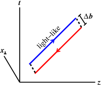
Figure 6: A Wilson loop with transverse separation $\Delta b$ and long, light-like sides.

There are many subtle details to contend with if one wants to make the Wilson loop definition precise. One consideration is how exactly to implement the different time-ordering prescriptions of the blue and red lines while keeping the Wilson loop gauge invariant Benzke , but that’s a detail that we’ll be able to ignore. Another, related consideration is whether one should think of the light-like Wilson loop of fig. 6 as a limiting case of slightly time-like Wilson loops or of slightly space-like Wilson loops. Though one may mostly read this paper without worrying about this detail, a little discussion here may clarify some later arguments. Physically, the particles represented by the long sides of the Wilson loop are moving slightly slower than the speed of light (at the very least because of medium-induced masses). On the other hand, as explained by Caron-Huot in ref. simon , a very slightly space-like loop is also sensitive to the contributions to $\hat{q}$ [or more generally $C(b)$] that are due to scattering of the high-energy particles from pre-existing fluctuations in the gauge fields of the medium. That includes, for example, all the physics of elastic scattering from the medium. For the slightly space-like loop, lack of causal connection implies that operators at different points on the loop commute with each other, and so it matters not how the lines of the loop are time ordered. This will be an advantage later on for making certain generic arguments. (It is also the definition relevant to a recent method for extracting $C(b)$ from lattice simulations for weakly-coupled quark-gluon plasmas nonpertCb1 ; nonpertCb2 .) However, when it comes to calculating the soft radiation effect $\delta\hat{q}$, we must instead think of the slightly time-like loop. And we will see later that how the lines are time-ordered impacts the values of different $\delta\hat{q}$’s arising in later application of soft corrections to energy loss.

Overall, I will consider the bare $\hat{q}$ to be defined by the slightly space-like loop (so that time-ordering does not matter), with the additional caveat that (at the very least) no radiation effects corresponding to $\omega_{y}>y_{\rm cut}E$ will be included in the bare $\hat{q}$, since $y_{\rm cut}E<\omega_{y}\ll\omega_{x}$ is going to represent the soft radition (with IR cut-off) effects that will define $\delta\hat{q}$. Fortunately, a more rigorous definition of bare $\hat{q}$, and its separation from $\delta\hat{q}$, will not be necessary for my purpose in this paper.

3.2.2 LMW’s calculation

Imagine that $\hat{q}$ is initially determined from scattering of the hard particles from the medium, as in fig. 1a. LMW’s calculation of the soft radiative corrections of fig. 1b was equivalent to computing the diagrams shown in fig. 7. In this language, their result was that the soft-radiation correction to the initial potential (17) is

$$\delta V_{{\scriptscriptstyle\rm LMW}}(\Delta b)=-\frac{i}{4}\delta\hat{q}(\Delta b)\times(\Delta b)^{2},$$ (19)

with $\delta\hat{q}(\Delta b)$ given by (12a). Since that $\delta\hat{q}(\Delta b)$ depends logarithmically on $\Delta b$, it does not have a finite limit as $\Delta b\to 0$. That is, $\delta V_{\rm LMW}$ is proportional to $\bigl{[}\ln(\Delta b)+{\rm const}\bigr{]}(\Delta b)^{2}$ at small $\Delta b$, not a truly quadratic potential. In any application, the value of $\delta\hat{q}$ will depend logarithmically on the relevant scale of $\Delta b$ as so on the relevant scale of $\Delta b$’s Fourier conjugate, $q_{\perp}$.

This situation has long been known to arise even in the context of leading-order perturbative calculations of the original elastic-scattering $\hat{q}$ for a weakly-coupled quark-gluon plasma (when running of the coupling is not included). In that case, it is an issue related to large-$q_{\perp}$ tails of the differential Rutherford scattering cross-section and to the fact that, mathematically, asking for the formal expectation $\langle p_{\perp}^{2}\rangle$ (which can be dominated by very rare events with very large $p_{\perp}$) can be a very different question than asking for the “typical” or median value of $p_{\perp}^{2}$. One may resolve these issues in the context of $p_{\perp}$ broadening, as briefly mentioned by LMW. We will not need to think about this at all, however. For the application of this paper, I will show that the LMW result (12) for $\delta\hat{q}(\Delta b)$ can be used as is, without any ambiguity of interpretation.

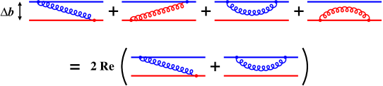
Figure 7: The diagrams underlying the LMW calculation. The Wilson lines and the radiated soft gluon line are all implicitly interacting with the medium.

3.3 A seeming disconnect

The problem with immediately making a connection between the LMW single log coefficient (12b) for soft radiative corrections to $p_{\perp}$ broadening and the single log coefficient (10b) extracted from soft corrections to hard splitting processes is that the LMW coefficient depends on one separation $\Delta b$. For the hard splitting process, there are three different, relevant transverse separations

$${\bm{b}}_{ij}\equiv{\bm{b}}_{i}-{\bm{b}}_{j}$$ (20)

as depicted in fig. 8. Moreover, these separations are not fixed: they are functions of time. Quantum mechanically, one must sum over all paths the three particles can take during the emission process. In order to see how to make use of the LMW result to include soft corrections, we need to first drill down and review some details of the usual leading-order BDMPS-Z calculation of the underlying hard splitting rate.

Figure 8: The hard splitting rate diagram, with emphasis on the three different transverse separations $b_{ij}$. The longitudinal momentum fraction labels $(x_{1},x_{2},x_{3})$ are shown for later reference.

4 Review: Leading-order BDMPS-Z splitting rates in $\hat{q}$ approximation

4.1 The “Hamiltonian”

I’ll use Zakharov’s version of the BDMPS-Z formalism for splitting rates. This corresponds to thinking of the three lines in fig. 3 (two particles in the amplitude and one in the conjugate amplitude) as a total of three particles evolving forward in time. Zakharov then treats the evolution as, formally, a type of quantum mechanics problem. A quick, heuristic way to understand the basic formulation is to first ignore interactions with the medium. In that case, the two particles in the amplitude will evolve quantum mechanically as $e^{-i\varepsilon_{1}t}$ and $e^{-i\varepsilon_{2}t}$, where, for high-energy particles moving nearly collinear with the $z$ axis,

$$\varepsilon_{i}\simeq\sqrt{p_{z}^{2}+p_{\perp}^{2}}\simeq|p_{z}|+\frac{p_{\perp}^{2}}{2|p_{z}|}\,.$$ (21)

The one particle in the conjugate amplitude evolves instead as $(e^{-i\varepsilon_{3}t})^{*}=e^{+i\varepsilon_{3}t}$. Altogether, the free system evolves as $e^{-iHt}$ with $H=\frac{p_{\perp 1}^{2}\vphantom{\big{|}}}{2|p_{z_{1}}|}+\frac{p_{\perp 2}^{2}\vphantom{\big{|}}}{2|p_{z_{2}}|}-\frac{p_{\perp 3}^{2}\vphantom{\big{|}}}{2|p_{z_{3}}|}.$ Now include (medium-averaged) interactions with the medium by including a three-body “potential” analogous to the two-body potential $V(\Delta b)$ discussed previously:

$$H=\frac{p_{\perp 1}^{2}}{2|p_{z_{1}}|}+\frac{p_{\perp 2}^{2}}{2|p_{z_{2}}|}-\frac{p_{\perp 3}^{2}}{2|p_{z_{3}}|}+V_{(3)}({\bm{b}}_{1},{\bm{b}}_{2},{\bm{b}}_{3}),$$ (22)

where ${\bm{b}}_{i}$ are the 2-dimensional transverse positions of the particles conjugate to ${\bm{p}}_{\perp i}$. There are various situations, such as (i) the weakly-coupled limit of a quark gluon plasma or (ii) the large-$N_{\rm c}$ limit, where one may argue that the 3-body potential decomposes into a sum of 2-body potentials. However, in the context of the harmonic oscillator (i.e. $\hat{q}$) approximation to potentials, there is a very simple, completely general argument: Any quadratic potential that is invariant under translations and rotations in the transverse plane can be written in the form

$$V_{(3)}({\bm{b}}_{1},{\bm{b}}_{2},{\bm{b}}_{3})=c_{12}b_{12}^{2}+c_{23}b_{23}^{2}+c_{31}b_{31}^{2}$$ (23)

for some constants $c_{ij}$.

In this paper, I will focus on the case of $g{\to}gg$ splitting since that’s the underlying hard process for the soft radiation single log coefficient (10b) that I eventually want to reproduce from LMW’s corrections to momentum broadening. In that case, the usual decomposition used in the literature would correspond to

$$V_{(3)}({\bm{b}}_{1},{\bm{b}}_{2},{\bm{b}}_{3})=-\tfrac{i}{8}\hat{q}_{\rm A}(b_{12}^{2}+b_{23}^{2}+b_{31}^{2}).$$ (24)

The coefficients in (24) can be motivated in various ways, such as from arguments for weakly-coupled plasmas. However, I will now review a more general argument in the context of the $\hat{q}$ approximation (adapted, with some additional clarification, from refs. 2brem ; Vqhat ).

I mentioned earlier the technical point that I was taking my bare $\hat{q}$ values to be defined by the light-like limit of slightly space-like Wilson loops, and that time-ordering prescriptions were then unimportant. As far as $\hat{q}$ values are concerned, there is then no difference between amplitude (blue) and conjugate amplitude (red) lines in fig. 3. For $g{\to}gg$ splitting, the (bare) 3-body potential in (23) must then be completely symmetric under permutations, so that

$$V_{(3)}=c(b_{12}^{2}+b_{23}^{2}+b_{31}^{2}).$$ (25)

(We will see later that this type of symmetry argument does not work exactly for soft radiative corrections, where time ordering matters.) Since the three high-energy particles in fig. 3 must form a color singlet (after medium averaging), the combined color representation of gluons 1 and 2 is forced to be in the adjoint representation so that that pair can form a color singlet with gluon 3. Now consider the limiting case of (25) where ${\bm{b}}_{1}={\bm{b}}_{2}$. Then the combination of gluons 1 and 2, which are on top of each other, is indistinguishable from a single gluon at that location. The 3-gluon system is then equivalent to a 2-gluon system, and so (25) with ${\bm{b}}_{1}={\bm{b}}_{2}$ must reproduce the gluon case $-\tfrac{i}{4}\hat{q}_{\rm A}b^{2}$ of the 2-particle potential (17). That fixes the coefficient $c$ of the 3-body harmonic oscillator potential (25) to give (24).

It will be useful to now introduce some notation that I will use throughout the paper. For the hard, single splitting $E\to xE,(1{-}x)E$, I define the longitudinal momentum fractions

$$(x_{1},x_{2},x_{3})\equiv(1{-}x,x,-1).$$ (26)

$x_{i}$ is defined to show the flow of $p_{zi}\simeq x_{i}E$ forward in the time as defined by the arrows in fig. 8. Note that the particle in the conjugate amplitude (red) has negative $x_{3}$ in this convention.

The final step of setting up the BDMPS-Z calculation is to simplify the 3-particle problem to an effective 1-particle problem by using symmetries of the problem. One may use transverse translation invariance to eliminate one particle degree of freedom by separating out what in ordinary 2-dimensional quantum mechanics would be the “center of mass” motion. It turns out that one may also use invariance of the original problem under tiny rotations that change the direction of the $z$ axis to eliminate a second particle degree of freedom. The result is that ${\bm{b}}_{12}$, ${\bm{b}}_{23}$ and ${\bm{b}}_{31}$ may be expressed in terms of a single 2-dimensional degree of freedom ${\bm{B}}$, with

$${\bm{b}}_{12}=(x_{1}{+}x_{2}){\bm{B}}=-x_{3}{\bm{B}},\quad{\bm{b}}_{23}=(x_{2}{+}x_{3}){\bm{B}}=-x_{1}{\bm{B}},\quad{\bm{b}}_{31}=(x_{3}{+}x_{1}){\bm{B}}=-x_{2}{\bm{B}}.$$ (27)

The momentum conjugate to ${\bm{B}}$ is

$${\bm{P}}=x_{2}{\bm{p}}_{\perp 1}-x_{1}{\bm{p}}_{\perp 2}=x_{3}{\bm{p}}_{\perp 2}-x_{2}{\bm{p}}_{\perp 3}=x_{1}{\bm{p}}_{\perp 3}-x_{3}{\bm{p}}_{\perp 1}.$$ (28)

With this reduction, the “Hamiltonian” given by (22) and (24) reduces to a single, 2-dimensional harmonic oscillator

$$H=\frac{P^{2}}{2M_{0}}+\tfrac{1}{2}M_{0}\Omega_{0}^{2}B^{2}$$ (29)

with

$$M_{0}=|x_{1}x_{2}x_{3}|E=x(1{-}x)E,$$ (30)

and (for $g{\to}gg$)

$$\Omega_{0}=\sqrt{-\frac{i\hat{q}_{\rm A}}{2E}\Bigl{(}\frac{1}{x_{1}}+\frac{1}{x_{2}}+\frac{1}{x_{3}}\Bigr{)}}=\sqrt{-\frac{i\hat{q}_{\rm A}(1{-}x{+}x^{2})}{x(1{-}x)E}}.$$ (31)

Note that $M_{0}$ and $\Omega_{0}$ are both symmetric under permutation of the three momentum fractions $(x_{1},x_{2},x_{3})$.

4.2 The calculation

Figure 9: The hard splitting rate. The shaded region indicates the region of time evolution between the two vertices, which is described by the 2-dimensional “quantum mechanics” Hamiltonian $H$.

Following Zakharov’s formulation Zakharov2 , the rate is given schematically in fig. 9 which, in my notation, translates to

$$\left[\frac{d\Gamma}{dx}\right]_{\rm LO}=\frac{\alpha_{\rm s}P(x)}{M_{0}^{2}}\operatorname{Re}\int_{0}^{\infty}\!\!d(\Delta t)\>{\bm{\nabla}}_{\bm{B}}\cdot{\bm{\nabla}}_{{\bm{B}}^{\prime}}\langle{\bm{B}},\Delta t|{\bm{B}}^{\prime},0\rangle\Bigl{|}_{{\bm{B}}=0={\bm{B}}^{\prime}}.$$ (32)

Here, the subscript “LO” stands for leading order in powers of “bremsstrahlung $\alpha_{\rm s}$.” The factor $\langle{\bm{B}},\Delta|{\bm{B}}^{\prime},0\rangle$ corresponds to time evolution in the shaded region of fig. 9 and is given by the quantum mechanics propagator associated with the Hamiltonian (29). In the $\hat{q}$ approximation I am using in this paper, this is simply a standard harmonic oscillator propagator, which in two dimensions is

$$\langle{\bm{B}},\Delta t|{\bm{B}}^{\prime},0\rangle=\frac{M_{0}\Omega_{0}\csc(\Omega_{0}\Delta t)}{2\pi i}\,\exp\Bigl{(}\tfrac{i}{2}M_{0}\Omega_{0}\bigl{[}(B^{2}{+}B^{\prime 2})\cot(\Omega_{0}\Delta t)-2{\bm{B}}\cdot{\bm{B}}^{\prime}\csc(\Omega_{0}\Delta t)\bigr{]}\Bigr{)}.$$ (33)

The derivatives, the overall factor of $\alpha_{\rm s}$, and the DGLAP splitting function $P(x)$ in (32) come from the two high-energy splitting vertices in the diagram. The current that a transversely-polarized gluon couples to in the collinear limit relevant to high energies is proportional to the transverse momentum. Correspondingly, in momentum space, the derivatives in (32) correspond to factors of ${\bm{P}}$, which characterize transverse momentum and which become $-i{\bm{\nabla}}$ in ${\bm{B}}$ space. The factor of $1/M_{0}^{2}$ in (32) arises from various normalization factors.

Using (33) in (32) and integrating over $\Delta t$ then yields

$$\left[\frac{d\Gamma}{dx}\right]_{\rm LO}=\frac{\alpha_{\rm s}P(x)}{\pi}\operatorname{Re}(i\Omega_{0}).$$ (34)

For the case of $g{\to}gg$, (31) then gives the final, standard result

$$\left[\frac{d\Gamma}{dx}\right]_{\rm LO}=\frac{\alpha_{\rm s}P_{g\to gg}(x)}{2\pi}\sqrt{\frac{\hat{q}_{\rm A}(1{-}x{+}x^{2})}{x(1{-}x)E}}$$ (35)

quoted earlier for the $\hat{q}$ approximation in an infinite medium.

5 Incorporating LMW $\hat{q}$ corrections into the BDMPS-Z calculation

5.1 Setup

The idea is to incorporate the LMW corrections to $\hat{q}$ into the 3-gluon potential (24) used for the BDMPS-Z calculation, choosing the $\Delta b$ in LMW to be the $b_{ij}$ appearing, respectively, in each term of the potential:

$$V_{(3)}^{\rm eff}({\bm{b}}_{1},{\bm{b}}_{2},{\bm{b}}_{3})=-\tfrac{i}{8}\Bigl{[}\hat{q}_{\rm A}^{\rm eff}(b_{12})\,b_{12}^{2}+\hat{q}_{\rm A}^{\rm eff}(b_{23})\,b_{23}^{2}+\hat{q}_{\rm A}^{\rm eff}(b_{31})\,b_{31}^{2}\Bigr{]}.$$ (36)

The assumption here that the $\hat{q}_{\rm A}^{\rm eff}$ in the first term cares only about the separation $b_{12}$ can be justified in the large-$N_{\rm c}$ limit.

To see this, imagine re-drawing the original $g{\to}gg$ time-ordered rate diagram of fig. 3b as a triangular cross-section lozenge, as in fig. 10a. The large-$N_{\rm c}$ requirement that diagrams be planar can be understood as a requirement that any additions to fig. 10a must lie on the surface of the lozenge without crossing lines. (The surface of the lozenge is topologically equivalent to a 2-sphere, which can be stereographically projected onto a plane. So any diagram that can be drawn on the lozenge’s surface without crossing lines can be mapped to a planar diagram.) Now consider, in particular, a soft correction to the hard splitting, as in fig. 2. Fig. 10b gives an example, where the soft curly gluon line connects lines 1 and 3. In the large-$N_{\rm c}$ limit, the soft line must then lie along the corresponding face of the lozenge. Correlations of interactions with the medium may be represented by a network of medium gluon correlators connecting to the high-energy particles. In large-$N_{\rm c}$, these correlations (brown lines in the figure) must also lie on the surface of the lozenge. That means that the soft gluon in fig. 10b only has medium correlations with particles 1 and 3 in this example. That soft gluon line is not affected at all by particle 2 and so only knows about the separation ${\bm{b}}_{31}$ between particles 1 and 3. Fig. 10b represents a correction to direct medium correlations between particles 1 and 3 and so represents a correction to the $\hat{q}_{\rm A}b_{13}^{2}$ term of the original potential (24). In summary, the first term in the corrected potential (36) depends only on $b_{31}$ in the large-$N_{\rm c}$ limit.

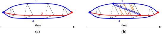
Figure 10: (a) A redrawing of the time-ordered $g{\to}gg$ hard splitting diagram of fig. 3b, depicted here as a 3-dimensional lozenge with triangular cross-section. In the large-$N_{\rm c}$ limit, additions to this diagram representing interactions must be drawable on the surface of the lozenge. The black triangles are just a visual aid, representing cross-sections of the lozenge at instants in time. (b) An example of a soft correction (curly gluon line), along with an example of medium correlations represented by the brown lines. Both 2-point and higher-point correlations are shown by way of example, but the analysis in this paper only assumes that the correlation length of the medium is small compared to formation times, not that the medium is weakly-coupled. Drawing the soft correction and correlators on the surface of the lozenge is just an abstraction for the sake of discussing the dominant time-ordered diagrammatic contributions in the large-$N_{\rm c}$ limit: there is no implication that the physical path of these lines must follow such a surface in transverse position space ${\bm{b}}$.

We now need to repeat the BDMPS-Z calculation using the effective potential (36) that includes LMW soft-radiative corrections to $\hat{q}$. This is no longer a harmonic oscillator problem, but we can still get a relatively simple answer to first order in the high-energy splitting $\alpha_{\rm s}$ by expanding around the usual BDMPS-Z $\hat{q}$-approximation result using time-ordered quantum mechanical perturbation theory in the correction $\delta V$ to the original potential $V_{(3)}$:

$$\delta V_{(3)}({\bm{b}}_{1},{\bm{b}}_{2},{\bm{b}}_{3})=-\tfrac{i}{8}\Bigl{[}\delta\hat{q}_{\rm A}^{\scriptscriptstyle{\scriptscriptstyle\rm LMW}}\!(b_{12})\,b_{12}^{2}+\delta\hat{q}_{\rm A}^{{\scriptscriptstyle\rm LMW}}\!(b_{23})\,b_{23}^{2}+\delta\hat{q}_{\rm A}^{{\scriptscriptstyle\rm LMW}}\!(b_{31})\,b_{31}^{2}\Bigr{]}.$$ (37)

Using the reduction (27) of the 3-particle problem to an effective 1-particle problem, that’s

$$\delta V_{(3)}(B)=-\tfrac{i}{8}\Bigl{[}\delta\hat{q}_{\rm A}^{{\scriptscriptstyle\rm LMW}}\!(|x_{3}|B)\,(x_{3}B)^{2}+\delta\hat{q}_{\rm A}^{{\scriptscriptstyle\rm LMW}}\!(|x_{1}|B)\,(x_{1}B)^{2}+\delta\hat{q}_{\rm A}^{{\scriptscriptstyle\rm LMW}}\!(|x_{2}|B)\,(x_{2}B)^{2}\Bigr{]}.$$ (38)

First order perturbation theory for (32) corresponds to

$$\delta\left[\frac{d\Gamma}{dx}\right]=\frac{\alpha_{\rm s}P(x)}{M_{0}^{2}}\operatorname{Re}\int_{0}^{\infty}\!\!d(\Delta t)\int_{0}^{\Delta t}dt_{1}\int d^{2}B_{1}\>\\ \times{\bm{\nabla}}_{\bm{B}}\cdot{\bm{\nabla}}_{{\bm{B}}^{\prime}}\Bigl{[}\underbrace{\langle{\bm{B}},\Delta t|{\bm{B}}_{1},t_{1}\rangle}_{\text{HO osc.}}\bigl{(}-i\,\delta V_{(3)}(B_{1})\bigr{)}\underbrace{\langle{\bm{B}}_{1},t_{1}|{\bm{B}}^{\prime},0\rangle}_{\text{HO osc.}}\Bigr{]}\Big{|}_{{\bm{B}}=0={\bm{B}}^{\prime}}\,,$$ (39)

which I’ve depicted schematically in fig. 11. It’s convenient to switch integration variables to $(t,t^{\prime})\equiv(\Delta t{-}t_{1},-t_{1})$ and then reorganize (39) as

$$\delta\left[\frac{d\Gamma}{dx}\right]=\frac{\alpha_{\rm s}P(x)}{M_{0}^{2}}\operatorname{Re}\biggl{\{}-i\int d^{2}B_{1}\left[\int_{0}^{\infty}dt\>{\bm{\nabla}}_{\bm{B}}\langle{\bm{B}},t|{\bm{B}}_{1},0\rangle\right]_{{\bm{B}}=0}\\ \cdot\left[\int_{-\infty}^{0}dt^{\prime}\>{\bm{\nabla}}_{{\bm{B}}^{\prime}}\langle{\bm{B}}_{1},0|{\bm{B}}^{\prime},t^{\prime}\rangle\right]_{{\bm{B}}^{\prime}=0}\delta V_{(3)}(B_{1})\biggr{\}}.$$ (40)

Using the harmonic oscillator propagator (33), the time integrals give

$$\left[\int_{0}^{\infty}dt\>{\bm{\nabla}}_{\bm{B}}\langle{\bm{B}},t|{\bm{B}}_{1},0\rangle\right]_{{\bm{B}}=0}=-\frac{iM_{0}{\bm{B}}_{1}}{\pi B_{1}^{2}}e^{-\frac{1}{2}M_{0}\Omega_{0}B_{1}^{2}}=\left[\int_{-\infty}^{0}dt_{1}\>{\bm{\nabla}}_{{\bm{B}}^{\prime}}\langle{\bm{B}}_{1},0|{\bm{B}}^{\prime},t^{\prime}\rangle\right]_{{\bm{B}}^{\prime}=0},$$ (41)

and so (40) simplifies to

$$\delta\left[\frac{d\Gamma}{dx}\right]=\frac{\alpha_{\rm s}P(x)}{\pi^{2}}\operatorname{Re}\biggl{\{}i\int\frac{d^{2}B_{1}}{B_{1}^{2}}\>e^{-M_{0}\Omega_{0}B_{1}^{2}}\,\delta V_{(3)}(B_{1})\biggr{\}}.$$ (42)

Figure 11: First-order perturbative correction to the integrand of the leading-order hard splitting rate in fig. 9.

5.2 First (naive) calculation

Now use (42) with the $\delta V_{(3)}$ of (38) and the LMW soft radiative correction (12) to $\hat{q}$. For the moment, I will use (12) for all of the $\delta\hat{q}$’s. But we will need to revisit that choice later for $\delta\hat{q}(b_{12})$, which involves two blue lines in fig. 10a rather than a blue line paired with a red line.

Because of the symmetric treatment of different pairs of the hard particles in the $\delta V_{(3)}$ potential (38), it’s useful to correspondingly break up the rate correction (42) into the terms coming from each such pair:

$$\delta\left[\frac{d\Gamma}{dx}\right]=\delta\left[\frac{d\Gamma}{dx}\right]_{12}+\delta\left[\frac{d\Gamma}{dx}\right]_{23}+\delta\left[\frac{d\Gamma}{dx}\right]_{31}$$ (43a)

with

$$\delta\left[\frac{d\Gamma}{dx}\right]_{ij}=\frac{\alpha_{\rm s}P(x)}{8\pi^{2}}x_{k}^{2}\operatorname{Re}\int d^{2}B_{1}\>e^{-M_{0}\Omega_{0}B_{1}^{2}}\,\delta\hat{q}_{\rm A}^{\scriptscriptstyle\rm LMW}\!(|x_{k}|B_{1}).$$ (43b)

Above and hereafter, $k$ refers to the index $1,2,3$ that is different from both $i$ and $j$. Applying (12a), I’ll write (43) using the notation

$$\delta\left[\frac{d\Gamma}{dx}\right]_{ij}=\int_{y\ll x}dy\>\left[\frac{d\Gamma}{dx\,dy}\right]_{ij},$$ (44)

with

$$\left[\frac{d\Gamma}{dx\,dy}\right]_{ij}=-\frac{C_{\rm A}\alpha_{\rm s}^{2}P(x)}{16\pi^{2}y}x_{k}^{2}\hat{q}_{\rm A}\operatorname{Re}\int_{0}^{\infty}d(B_{1}^{2})\>e^{-M_{0}\Omega_{0}B_{1}^{2}}\bigl{[}\ln y+\bar{s}_{\scriptscriptstyle\rm LMW}(|x_{k}|B_{1})\bigr{]}$$ (45)

in the small-$y$ limit relevant to the soft radiative corrections (44). (The notation $d\Gamma/dx\,dy$ also makes contact with the notation of refs. qcd ; logs for double splitting with overlapping formation times.) With (12b) for $\bar{s}_{\scriptscriptstyle\rm LMW}$, the $B_{1}^{2}$ integral in (45) is straightforward, giving

$$\left[\frac{d\Gamma}{dx\,dy}\right]_{ij}=-\frac{C_{\rm A}\alpha_{\rm s}^{2}P(x)}{4\pi^{2}y}\operatorname{Re}\left\{\frac{x_{k}^{2}\hat{q}_{\rm A}}{4M_{0}\Omega_{0}}\left[\ln y+2\ln\left(\frac{x_{k}^{2}}{4M_{0}\Omega_{0}}\sqrt{\tfrac{1}{2}\hat{q}_{\rm A}E}\right)\right]\right\}.$$ (46)

This result can be algebraically manipulated into a nicer form by using (31) to show that

$$\frac{x_{k}^{2}\hat{q}_{\rm A}}{4M_{0}\Omega_{0}}=iw_{ij}\Omega_{0}$$ (47)

with

$$w_{ij}\equiv\frac{x_{k}^{2}}{x_{1}^{2}+x_{2}^{2}+x_{3}^{2}}\,.$$ (48)

By definition, the $w_{ij}$ have the property that

$$w_{12}+w_{23}+w_{31}=1,$$ (49)

and we’ll see later that it is useful to think of them as relative weights of various contributions (hence the choice of letter “$w$”). For now, use (47) to rewrite (46) as

$$\left[\frac{d\Gamma}{dx\,dy}\right]_{ij}=-\frac{C_{\rm A}\alpha_{\rm s}^{2}P(x)}{4\pi^{2}y}\,w_{ij}\operatorname{Re}\left\{i\Omega_{0}\left[\ln y+2\ln\left(iw_{ij}\Omega_{0}\sqrt{E/2\hat{q}_{\rm A}}\right)\right]\right\}.$$ (50)

Knowing the complex phase of $\Omega_{0}=e^{-i\pi/4}|\Omega_{0}|$, this can be rewritten as

$$\left[\frac{d\Gamma}{dx\,dy}\right]_{ij}=-\frac{C_{\rm A}\alpha_{\rm s}}{4\pi y}\,w_{ij}\left[\frac{d\Gamma}{dx}\right]_{\rm LO}\left[\ln y+2\ln\left(w_{ij}|\Omega_{0}|\sqrt{E/2\hat{q}_{\rm A}}\right)-\frac{\pi}{2}\right]$$ (51)

in terms of the BDMPS-Z rate $[d\Gamma/dx]_{\rm LO}$ given by (34). The $\pi/2$ term arises from the logarithm of the complex phase in (50) [in combination with the operation $2\operatorname{Re}\{i\Omega_{0}\cdots\}$]. The corresponding single-log coefficient $\bar{s}(x)$ appearing in (10a) for soft radiative corrections to hard $g{\to}gg$ splitting would then be

$$\bar{s}=\bar{s}_{12}+\bar{s}_{23}+\bar{s}_{31}$$ (52)

with

$$\bar{s}_{ij}=w_{ij}\left[2\ln\left(w_{ij}|\Omega_{0}|\sqrt{E/2\hat{q}_{\rm A}}\right)-\frac{\pi}{2}\right].$$ (53)

Using the explicit values $(x_{1},x_{2},x_{3})=(1{-}x,x,-1)$ of the three longitudinal momentum fractions, and using the formula (31) for $\Omega_{0}$, one may algebraically manipulate this result into a form similar to the coefficient (10b) extracted from the soft-$y$ limit of difficult generic-$y$ calculations in ref. logs . By having instead repeated BDMPS-Z using the LMW correction to $\hat{q}$, we obtain here the slightly different result

$$\bar{s}(x)=-\ln\bigl{(}16\,x(1{-}x)(1{-}x{+}x^{2})\bigr{)}+2\,\frac{\bigl{[}x^{2}\bigl{(}\ln x-\frac{\pi}{8}\bigr{)}+(1{-}x)^{2}\bigl{(}\ln(1{-}x)-\frac{\pi}{8}\bigr{)}{{\color[rgb]{1,0,0}{}-\frac{\pi}{8}}}\bigr{]}}{(1-x+x^{2})}.$$ (54)

This result matches (10b) except for the very last $\pi/8$ term above (in red). This discrepancy originates from the $\pi/2$ term in (53) for the particular case of $\bar{s}_{12}$.

5.3 Fixing up amplitude-amplitude $\delta\hat{q}(b_{12})$

As mentioned earlier, LMW’s calculation LMW of soft radiative corrections to $p_{\perp}$ broadening corresponds to studying the rate of $p_{\perp}$ change for a single particle, and a rate involves an amplitude for the particle (a blue line in my conventions) multiplied by a conjugate amplitude for that particle (a red line). However, in the previous derivation, in one place I used LMW’s formula for $\delta\hat{q}$ to treat soft radiation between two particles in the amplitude (two blue lines). We now need to go back and fix that up. Fortunately, LMW’s derivation can be adapted to this case.

The top line of fig. 12 shows the analog, for two amplitude Wilson lines, of my depiction of LMW’s diagrams in fig. 7. By rotation invariance about the direction of the Wilson lines, the sum can be rewritten as in the second line of fig. 12. Finally, LMW’s calculation is determined by the soft gluon propagator. It matters whether that propagator is in the amplitude or conjugate amplitude (blue or red), which it inherits in these diagrams from the first vertex it is emitted from. In the last two lines of fig. 12, it does not matter whether the lower Wilson line is colored blue or red. By comparing the last line of this figure to the LMW case of fig. 7, we then see that the result is the same except that one should not take the real part $\operatorname{Re}(\cdots)$ at the end. We can use the derivation from LMW’s paper LMW if we (i) avoid ever taking the real part and, correspondingly, (ii) are very careful to keep track of complex phases in their derivation. See appendix A for details. The result is that (12b) is modified to

$$\bar{s}_{\mbox{\scriptsize blue-blue}}(\Delta b)=2\ln\Bigl{(}\tfrac{1}{4}(\Delta b)^{2}\sqrt{\tfrac{1}{2}\hat{q}_{\rm A}E}\,e^{-i\pi/4}\Bigr{)}+2\gamma_{\rm\scriptscriptstyle E}.$$ (55)

The only difference is the factor of $e^{-i\pi/4}$ inside the argument of the logarithm, and so

$$\bar{s}_{\mbox{\scriptsize blue-blue}}(\Delta b)=\bar{s}_{\scriptscriptstyle\rm LMW}(\Delta b)-\frac{i\pi}{2}.$$ (56)

Now using this amplitude-amplitude soft correction in (45) in the case of $[d\Gamma/dx\,dy]_{12}$ gives

$$\left[\frac{d\Gamma}{dx\,dy}\right]_{12}=-\frac{C_{\rm A}\alpha_{\rm s}^{2}P(x)}{4\pi^{2}y}\operatorname{Re}\left\{\frac{x_{3}^{2}\hat{q}_{\rm A}}{4M_{0}\Omega_{0}}\left[\ln y+2\ln\left(\frac{x_{3}^{2}}{4M_{0}\Omega_{0}}\sqrt{\tfrac{1}{2}\hat{q}_{\rm A}E}\,e^{-i\pi/4}\right)\right]\right\}$$ (57)

instead of (46). The explicit $e^{-i\pi/4}$ above cancels the phase of $\Omega_{0}$ inside the logarithm, eliminating the $\pi$ terms in this case, so that the corresponding version of (53) is

$$\bar{s}_{12}=w_{12}\left[2\ln\left(w_{12}|\Omega_{0}|\sqrt{E/2\hat{q}_{\rm A}}\right)\right].$$ (58)

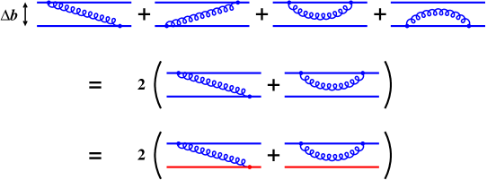
Figure 12: Similar to the diagrams of fig. 7 for the LMW correction, but here both Wilson lines are amplitude (blue) lines.

5.4 Total

Using (53) for blue-red pairs and (58) for the blue-blue pair, the total single log coefficient is

$$\bar{s}=\bar{s}_{12}+\bar{s}_{23}+\bar{s}_{31}\\ =w_{12}\left[2\ln\left(w_{12}|\Omega_{0}|\sqrt{E/2\hat{q}_{\rm A}}\right)\right]+w_{23}\left[2\ln\left(w_{23}|\Omega_{0}|\sqrt{E/2\hat{q}_{\rm A}}\right)-\frac{\pi}{2}\right]\\ +w_{31}\left[2\ln\left(w_{31}|\Omega_{0}|\sqrt{E/2\hat{q}_{\rm A}}\right)-\frac{\pi}{2}\right].$$ (59)

This now exactly reproduces the result (10b) extracted from the small-$y$ limit of generic-$y$ results for double splitting.

6 Other ways to write the final answer

Algebraically, the final answer (59) may be evocatively written directly in terms of the LMW single-log coefficient of (12b) as

$$\bar{s}=w_{12}\,\bar{s}_{\scriptscriptstyle\rm LMW}(\bar{b}_{12})+w_{23}\bigl{[}\bar{s}_{\scriptscriptstyle\rm LMW}(\bar{b}_{23})-\tfrac{\pi}{2}\bigr{]}+w_{31}\bigl{[}\bar{s}_{\scriptscriptstyle\rm LMW}(\bar{b}_{31})-\tfrac{\pi}{2}\bigr{]},$$ (60a)

where

$$\bar{b}_{ij}\equiv\sqrt{w_{ij}\,\frac{4|\Omega_{0}|}{e^{\gamma_{\rm\scriptscriptstyle E}}\hat{q}_{\rm A}}}$$ (60b)

may be interpreted as a typical separation of the indicated pair during the underlying hard splitting process.

For qualitative understanding of this formula, it will also be useful to use (47) and (48) to rewrite it in the form

$$\bar{s}=w_{12}\,\bar{s}_{\scriptscriptstyle\rm LMW}(|x_{3}\bar{B}|)+w_{23}\bigl{[}\bar{s}_{\scriptscriptstyle\rm LMW}(|x_{1}\bar{B}|)-\tfrac{\pi}{2}\bigr{]}+w_{31}\bigl{[}\bar{s}_{\scriptscriptstyle\rm LMW}(|x_{2}\bar{B}|)-\tfrac{\pi}{2}\bigr{]}$$ (61a)

with

$$\bar{B}\equiv\sqrt{\frac{1}{e^{\gamma_{\rm\scriptscriptstyle E}}M_{0}\Omega_{0}}}.$$ (61b)

I have no physical insight to offer about the $O(1)$ normalization factor $e^{\gamma_{\rm\scriptscriptstyle E}}$ in (60b) and (61b): I simply chose that normalization so that (60a) would reproduce (59). However, one may understand both the parametric scale and longitudinal momentum fraction $(x_{1},x_{2},x_{3})$ dependence of the $\bar{b}_{ij}=|x_{k}\bar{B}|$. First, consider the $x\ll 1$ case of the hard $g{\to}gg$ splitting (but $x\gg y$ so that $x$ is still hard compared to the soft corrections we have been computing). In that case, the $x_{2}{=}x$ gluon is the hard particle most deflected by the medium, and its deflection is what controls the formation time, so that $t_{\rm form}(x)\sim\sqrt{\omega_{x}/\hat{q}}=\sqrt{xE/\hat{q}}$. The transverse momentum kicks during the formation time of the hard splitting process are then of order $Q_{\perp}\sim\sqrt{\hat{q}t_{\rm form}}\sim(xE\hat{q})^{1/4}$, and the corresponding transverse separation scale should be $1/Q_{\perp}\sim(xE\hat{q})^{-1/4}$ for the separation of the easily-deflected $x_{2}{=}x$ gluon from the harder-to-deflect $x_{1}$ and $x_{3}$ gluons. So we expect

$$b_{13}\ll b_{12}\simeq b_{23}\sim(xE\hat{q})^{-1/4}\quad\mbox{for $x\ll 1$},$$ (62)

which is indeed the parametric behavior of (60b) in this limit. But we can make a more precise argument about the $x$ dependence, without assuming $x\ll 1$, by remembering that transverse separations are precisely related to the reduced variable ${\bm{B}}$ by (27): namely, $b_{ij}=|x_{k}{\bm{B}}|$. The variable ${\bm{B}}$, in turn, describes a harmonic oscillator with mass $M_{0}$ and frequency $\Omega_{0}$. For a quantum harmonic oscillator, the fundamental distance scale is parametrically $(M_{0}\Omega_{0})^{-1/2}$, as in (61b). So, in hindsight, we could have expected that the typical separations $b_{ij}$ would be proportional to the $\bar{b}_{ij}=|x_{k}\bar{B}|$ determined by (61b).

I originally introduced the weights $w_{ij}$ appearing in (60a) as the relative sizes (48) of squares of the longitudinal momentum fractions $(x_{1},x_{2},x_{3})$. For some insight into their role, use (60b) to re-express the weights in terms of the relative sizes of the typical squared transverse separations:

$$w_{ij}=\frac{\bar{b}_{ij}^{2}}{\vphantom{\bigl{|}^{*}}\bar{b}_{12}^{2}+\bar{b}_{23}^{2}+\bar{b}_{31}^{2}}\,.$$ (63)

Now consider the picture in fig. 13 of a soft emission from the three lines of an underlying hard emission. In this figure, the transverse separations of the hard lines are depicted near the time of the soft emission. Imagine two of those lines are relatively close together, as in the case $x\ll 1$ covered by (62). It will be harder for an even softer (and so long wavelength) emission $y$ to resolve the close pair $(3,1)$ than it is to resolve the less-close pairs $(1,2)$ and $(2,3)$. The weights (63) appearing in (60a) reflect the relative difficulty of the soft radiation to resolve these different pairs. Though I’ve been focused on the single logs, the same is true of the double logs. The $\ln y$ behavior in (10a), which generates the double log after integration with $dy/y$, also decomposes into contributions from different pairs as

$$\ln y=w_{12}\ln y+w_{23}\ln y+w_{31}\ln y.$$ (64)

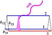
Figure 13: Soft radiation from three hard lines somewhere in the middle of a hard $g{\to}gg$ splitting process. This is a magnified view of one of the soft vertices in fig. 2, and here the magenta triangle is just a way to represent that the soft gluon can couple to any one of the three hard lines. This figure depicts the relative transverse positions of the lines during the soft emission process and shows the case of slightly small $x$, for which $x_{2}{=}x$ is typically the farthest away of the three hard lines.

One may wonder why the weights $w_{ij}$ in (60a) and (64) care about the relative size of $\bar{b}_{ij}^{2}$ rather than the size of $\bar{b}_{ij}^{2}$ directly. This is an artifact of having factored out the full leading-order rate $[d\Gamma/dx]_{\rm LO}$ in the definition (10a) of the soft corrections. Inserting a factor of $1=w_{12}{+}w_{23}{+}w_{31}$ and using (60b), the formula (34) for $[d\Gamma/dx]_{\rm LO}$ can be rewritten as

$$\left[\frac{d\Gamma}{dx}\right]_{\rm LO}=\frac{\alpha_{\rm s}P(x)}{4\pi\sqrt{2}}\,e^{\gamma_{\rm\scriptscriptstyle E}}\hat{q}_{\rm A}(\bar{b}_{12}^{2}+\bar{b}_{23}^{2}+\bar{b}_{31}^{2}).$$ (65)

Using this and (51), or alternatively returning to (46) and directly using $b_{ij}=|x_{k}\bar{B}|$ and (61b) (and in either case also including the proper phase from section 5.3 for the amplitude-amplitude pair $[d\Gamma/dx\,dy]_{12}$):

$$\delta\left[\frac{d\Gamma}{dx}\right]=\int_{y\ll x}dy\>\left[\frac{d\Gamma}{dx\,dy}\right],$$ (66)

with

$$\frac{d\Gamma}{dx\,dy}=\left[\frac{d\Gamma}{dx\,dy}\right]_{12}+\left[\frac{d\Gamma}{dx\,dy}\right]_{23}+\left[\frac{d\Gamma}{dx\,dy}\right]_{31}\\ =-\frac{C_{\rm A}\alpha_{\rm s}^{2}P(x)}{16\pi^{2}y\sqrt{2}}\,e^{\gamma_{\rm\scriptscriptstyle E}}\hat{q}_{\rm A}\Bigl{\{}\bar{b}_{12}^{2}\bigl{[}\ln y+\bar{s}_{\scriptscriptstyle\rm LMW}(\bar{b}_{12})\bigr{]}+\bar{b}_{23}^{2}\bigl{[}\ln y+\bar{s}_{\scriptscriptstyle\rm LMW}(\bar{b}_{23})-\tfrac{\pi}{2}\bigr{]}\\ +\bar{b}_{31}^{2}\bigl{[}\ln y+\bar{s}_{\scriptscriptstyle\rm LMW}(\bar{b}_{31})-\tfrac{\pi}{2}\bigr{]}\Bigr{\}}.$$ (67)

Alternatively, one may define a complex-valued

$$\beta_{ij}\equiv|x_{k}|\bar{B}$$ (68)

in terms of complex-valued $\bar{B}$ (61b). Then

$$\frac{d\Gamma}{dx\,dy}=-\frac{C_{\rm A}\alpha_{\rm s}^{2}P(x)}{16\pi^{2}y}\,e^{\gamma_{\rm\scriptscriptstyle E}}\hat{q}_{\rm A}\operatorname{Re}\Bigl{\{}\beta_{12}^{2}\bigl{[}\ln y+\bar{s}_{\mbox{\scriptsize\rm blue-blue}}(\beta_{12})\bigr{]}+\beta_{23}^{2}\bigl{[}\ln y+\bar{s}_{\scriptscriptstyle\rm LMW}(\beta_{23})\bigr{]}\\ +\beta_{31}^{2}\bigl{[}\ln y+\bar{s}_{\scriptscriptstyle\rm LMW}(\beta_{31})\bigr{]}\Bigr{\}},$$ (69a)

which writes the final answer in terms of just $$\bar{s}_{{\scriptscriptstyle\rm LMW}} \bar{s}_{\mbox{\scriptsize blue-blue}} \pi \bar{s}_{\scriptscriptstyle\rm LMW}$$ for red-blue pairs of lines and for blue-blue pairs of lines, without additional, explicitly written terms. Or one may compactly write everything in this form in terms of by noting

$$\operatorname{Re}\Bigl{\{}\beta_{12}^{2}\bigl{[}\ln y+\bar{s}_{\mbox{\scriptsize\rm blue-blue}}(\beta_{12})\bigr{]}\Bigr{\}}=\operatorname{Re}\Bigl{\{}\beta_{12}^{2}\bigl{[}\ln y+\bar{s}_{\scriptscriptstyle\rm LMW}\bigl{(}|\beta_{12}|\bigr{)}\bigr{]}\Bigr{\}}.$$ (69b)

7 Conclusion

We have seen that, at the “microscopic” level, using the $p_{\perp}$-broadening effective value of $\hat{q}_{\rm eff}$ inside the BDMPS-Z calculation of hard $g{\to}gg$ scattering correctly reproduces not only double logs but also the subleading, single-log soft radiative corrections to hard $g{\to}gg$ splitting. Using (65), (66) and (69), we can also express the final, soft-radiation corrected splitting rate in terms of the $p_{\perp}$-broadening effective $\hat{q}_{\rm eff}(\Delta b)=\hat{q}+\delta\hat{q}_{\scriptscriptstyle\rm LMW}(\Delta b)$ from (12a) as

$$\left[\frac{d\Gamma}{dx}\right]_{\rm LO}+\delta\left[\frac{d\Gamma}{dx}\right]=\frac{\alpha_{\rm s}P(x)}{4\pi}\,\operatorname{Re}\left\{\hat{\beta}_{12}^{2}\sqrt{\frac{\hat{q}_{\rm A}^{\rm eff}(|\beta_{12}|)}{E}}+\hat{\beta}_{23}^{2}\sqrt{\frac{\hat{q}_{\rm A}^{\rm eff}\bigl{(}\beta_{23}\bigr{)}}{E}}+\hat{\beta}_{31}^{2}\sqrt{\frac{\hat{q}_{\rm A}^{\rm eff}\bigl{(}\beta_{31}\bigr{)}}{E}}\,\right\}$$ (70a)

through first order in soft radiative corrections $$\delta\hat{q} \beta_{ij} \hat{\beta}_{ij}$$, with complex-valued transverse separation scales given in terms of dimensionless by

$$\beta_{ij}\equiv\frac{e^{-\gamma_{\rm\scriptscriptstyle E}/2}}{(\hat{q}_{\rm A}E)^{1/4}}\,\hat{\beta}_{ij}$$ (70b)

and

$$\begin{pmatrix}\hat{\beta}_{12}\\ \hat{\beta}_{23}\\ \hat{\beta}_{31}\end{pmatrix}\equiv(\hat{q}_{\rm A}E)^{1/4}\sqrt{\frac{1}{M_{0}\Omega_{0}}}\begin{pmatrix}|x_{3}|\\ |x_{1}|\\ |x_{2}|\end{pmatrix}=\frac{e^{-i\pi/8}}{\bigl{[}\tfrac{1}{2}x(1{-}x)(1{-}x{+}x^{2})]^{1/4}}\begin{pmatrix}1\\ 1{-}x\\ x\end{pmatrix}.$$ (70c)

Because of the complex phase in (70c), the $\hat{q}_{\rm A}^{\rm eff}\bigl{(}|\beta_{12}|\bigr{)}$ is not the same thing as $\hat{q}_{\rm A}^{\rm eff}(\beta_{12})$, breaking the symmetry between the three gluons in (70a). That means, at the level of soft radiative corrections, one can no longer ignore the difference between $\hat{q}^{\rm eff}$ effects for particle pairs with (i) both particles in the amplitude vs. (ii) one particle each in the amplitude and conjugate amplitude. For traditional BDMPS-Z based calculations in the $\hat{q}$ approximation, the possibility of such differences has always been ignored.

One of the side benefits of the result of this paper is that it provides a highly non-trivial cross-check of the very involved calculations of hard radiative corrections to $g{\to}gg$ in refs. 2brem ; seq ; dimreg ; QEDnf ; qcd , from which the limit of soft-radiative corrections was extracted in ref. logs . In particular, the “$\pi$ terms” in those results, such as the $\pi$ terms in (10b), required a great deal of fussy work to correctly choose branch cuts at intermediate stages of the calculation. It is reassuring to see everything match up exactly with the much simpler derivation here for the case of soft radiative corrections.

In this paper, I have used a sharp IR cut-off $y_{\rm cut}E$ on the softest radiative gluon (allowing coverage of at most the red region of fig. 5), because that was the explicit calculation logs that was available to compare to. Readers may wonder what would happen in a more complete calculation that also included the gray region of fig. 5 and correctly handled the breakdown of the $\hat{q}$ approximation at $\Delta t\sim\tau_{0}$. Similarly, one might want to include running of the $\alpha_{\rm s}$ associated with the soft splitting. My personal expectation is that the “microscopic” version of the universality of $\hat{q}$ shown in this paper will continue to hold (at least in the large-$N_{\rm c}$ limit). That is, I expect that if one repeated the BDMPS-Z derivation using the full $\hat{q}_{\scriptscriptstyle\rm LMW}(\Delta b)$ (now including the gray region and/or running of $\alpha_{\rm s}$), then one would obtain a result that correctly incorporated soft radiative corrections to hard splitting $g{\to}gg$. I expect this because, as in fig. 5, the time scales for soft radiation (and especially for the gray region) are small compared to the formation time $t_{\rm form}(x)$, and so the soft gluon curly line in fig. 10 extends only for a relatively short time, during which the hard-particle lines are approximately straight with approximately constant separation, just like in the calculation of the soft correction $\delta\hat{q}$ to transverse momentum broadening depicted in fig. 7 (or alternatively fig. 12). I believe that the basis for the calculation that I’ve made in this paper depends merely on this (large-$N_{\rm c}$) factorization, and not on the exact details of the formula for the soft correction. It would be interesting to explore to what extent the “macroscopic” final formula (70) might also be robust, were one to use the full $\hat{q}_{\scriptscriptstyle\rm LMW}(\Delta b)$ to redo the BDMPS-Z calculation.

Finally, a very interesting unresolved question is whether the results of this paper require the large-$N_{\rm c}$ approximation, or whether “microscopic universality” for sub-leading single logs holds for finite $N_{\rm c}$ as well.

Appendix A Complex phases in LMW’s derivation

LMW LMW were always interested in the real part of their diagrammatic results. Here, I clarify some of the complex phases in LMW’s derivation for the sake of my section 5.3, where the result is needed without taking the real part.

Like LMW’s discussion in their main text, I will work here in the large-$N_{\rm c}$ limit, even though their results for $\delta\hat{q}$ for transverse momentum broadening are more general and do not ultimately depend on this limit. Similarly, even though I am interested in soft radiative corrections to momentum broadening of gluons, here I will follow LMW and focus on corrections to momentum broadening of quarks. In the context of the large-$N_{\rm c}$ limit, their quark $\hat{q}$ is related to gluon $\hat{q}_{\rm A}$ by

$$\hat{q}=\frac{\hat{q}_{\rm A}}{2}\qquad\mbox{(large $N_{\rm c}$)}.$$ (71)

These details do not matter. If one did the same calculations for hard particles in any color representation $R$, one would find the same final formula for the relative correction $(\delta\hat{q}_{R})/\hat{q}_{R}$. By sticking to the case considered by LMW, however, the discussion will be simpler, and I will be able to more easily compare formulas.

Table 1 gives a translation between LMW’s notation and the notation I have used in the main text. To simplify direct comparison to their equations, I will mostly use LMW’s notation in this appendix. One exception has to do with the fact that part of LMW’s calculation is set up so that their propagator $G$ and complex frequency $\omega_{0}$ represent a situation where the soft gluon is first emitted in the conjugate amplitude — what in this paper I would draw as a red gluon. With my conventions, I am interested in handling the case where the soft gluon is emitted in the amplitude — a blue gluon. The relevant propagator and complex frequency are then $G^{*}$ and $\omega_{0}^{*}$ in LMW’s notation, which I will call ${\cal G}$ and $\Omega_{\rm s}$ (see table 1). The subscript on $\Omega_{\rm s}$ stands for “soft.”

LMW	this paper
$\omega$	$\omega_{y}{=}yE$
$x_{\perp}$	$\Delta b$
${\bm{B}}_{\perp}$	${\bm{b}}$ of the soft gluon
$t$	$\Delta t_{y}$
$N_{\rm c}$	$C_{\rm A}$ (= $2C_{\rm F}$ for $N_{\rm c}{\to}\infty$)
$\hat{q}$	see text
$\omega_{0}{\equiv}\sqrt{i\hat{q}/\omega}$	$\Omega_{\rm s}^{*}{\equiv}\left(\sqrt{i\hat{q}_{\rm A}/2\omega_{y}}\right)^{*}=\sqrt{-i\hat{q}_{\rm A}/2\omega_{y}}$
$G$	${\cal G}^{*}$
$G_{0}$	${\cal G}^{*}_{\rm vac}$
$l_{0}$	$\tau_{0}$

Table 1: Translations between the notation of LMW LMW and this paper.

A.1 Setup

LMW carry out different parts of their derivation in slightly different ways. In some parts [their calculation of single logs from boundary (b)], they implicitly treat the soft gluon as what I would call a red gluon (one emitted first from the conjugate amplitude). In other parts [their calculation of single logs from boundary (a)], their formulas implicitly treat it as what I would call a blue gluon (emitted first from the amplitude). None of that matters to their application, because they need to take $\operatorname{Re}(\cdots)$ at the end. But I additionally need the case where I do not take the real part. So, we need to first review the general starting formula from whence their single log contributions are extracted. Here, I will briefly summarize the origin of that formula in the language I have used in this paper. My starting formula will be a very minor variation of LMW’s.

Imagine computing the soft radiative correction to the amplitude-amplitude (blue-blue) potential, represented by fig. 12. As discussed in the main text, taking $\operatorname{Re}(\cdots)$ of the result will then be equivalent to LMW’s calculation.

Without radiative corrections, the light-like Wilson loop has length dependence proportional to

$$e^{-iV_{0}(x_{\perp})L}$$ (72)

where

$$V_{0}(x_{\perp})=-\tfrac{i}{4}\hat{q}x_{\perp}^{2}$$ (73)

as in (17). The first-order correction represented by fig. 12 is

$$\delta\left[e^{-iV(x_{\perp})L}\right]=-C_{\rm F}\kern 0.4ptg^{2}\int_{\rm soft}\frac{d\omega}{(2\pi)2\omega}\int_{0}^{L}dz_{2}\int_{0}^{z_{2}}dz_{1}\>e^{-iV_{0}(x_{\perp})\,(L{-}z_{2})}\\ \times\frac{{\bm{\nabla}}_{B_{1\perp}}\!\cdot{\bm{\nabla}}_{B_{2\perp}}}{\omega^{2}}\,{\cal G}({\bm{B}}_{2\perp},z_{2};{\bm{B}}_{1\perp},z_{1})e^{-iV_{0}(x_{\perp})\,z_{1}}\Biggl{|}_{{\bm{B}}_{2\perp}=0}^{{\bm{B}}_{2\perp}={\bm{x}}_{\perp}}\Biggl{|}_{{\bm{B}}_{1\perp}=0}^{{\bm{B}}_{1\perp}={\bm{x}}_{\perp}},$$ (74)

where $z_{1}$ and $z_{2}$ are the $z$ coordinates (equivalently times) of the first and second vertices. Above, the two factors of $e^{-iV_{0}(x_{\perp})\cdots}$ represent the contributions to the Wilson loop (i) from after $z_{2}$ and (ii) from before $z_{1}$. The $d\omega/[(2\pi)2\omega]$ comes from the usual relativistic phase space measure $d^{3}p/[(2\pi)^{3}2\omega]$ for the (approximately on-shell) soft gluon, the transverse $d^{2}p_{\perp}/(2\pi)^{2}$ part of which is absent because we are working in transverse position space instead of transverse momentum space. $C_{\rm F}$ is the quark quadratic Casimir

$$C_{\rm F}=\frac{N_{\rm c}}{2}\qquad\mbox{(large $N_{\rm c}$)}.$$ (75)

The $-C_{\rm F}\kern 0.4ptg^{2}\,{\bm{\nabla}}_{B_{1\perp}}\!\cdot{\bm{\nabla}}_{B_{2\perp}}/\omega^{2}$ comes from the vertices $igT_{\rm color}^{a}v\cdot A^{a}$ where the soft gluons attach to the Wilson lines, summed over transverse polarizations of the (nearly-collinear) soft gluon. The four different terms added/subtracted by the combinations of values of ${\bm{B}}_{1\perp}$ and ${\bm{B}}_{2\perp}$ indicated at the end of (74) represent the four diagrams in fig. 12. The ${\cal G}$ is the two-dimensional quantum mechanics Green function for the propagation of the soft gluon in the medium, in the $\hat{q}$ approximation, analogous to (33). In the LMW case where the hard particles are quarks rather than gluons, and where the quarks are taken to have fixed transverse positions $0$ and ${\bm{x}}_{\perp}$ as above, the analog of the 3-particle potential (24) is

$$V_{\rm(qgq)}(0,{\bm{b}},{\bm{x}}_{\perp})=-\tfrac{i}{8}\hat{q}_{\rm A}\bigl{[}|{\bm{b}}|^{2}+|{\bm{b}}-{\bm{x}}_{\perp}|^{2}\bigr{]}=-\tfrac{i}{4}\hat{q}\bigl{[}|{\bm{b}}|^{2}+|{\bm{b}}-{\bm{x}}_{\perp}|^{2}\bigr{]}\qquad\mbox{(large $N_{\rm c}$)},$$ (76)

in which ${\bm{b}}$ is the transverse position of the soft gluon. The $b_{31}^{2}$ term of (24) does not appear here because in the large-$N_{\rm c}$ limit the quarks cannot directly interact when there is a gluon between them. Up to conventions concerning complex conjugation, (76) is the potential that appears in LMW eq. (6). Complex conjugation arises because I consider the case of a gluon emitted first from the amplitude, whereas LMW eq. (6) implicitly refers to the case where the gluon is instead first emitted from the conjugate amplitude. As a result, the explicit formula for my propagator ${\cal G}$ in (74) is the complex conjugate $G^{*}$ of their formula for their propagator $G$ in LMW eq. (8).

In order to make contact with LMW’s starting formula, rewrite (74) above as

$$\delta\left[e^{-iV(x_{\perp})L}\right]=\int_{\rm soft}\frac{d\omega}{\omega}\>{\cal N}(x_{\perp},\omega)$$ (77a)

with

$${\cal N}(x_{\perp},\omega)\equiv-\frac{C_{\rm F}\kern 0.6pt\alpha_{\rm s}}{\omega^{2}}\int_{0}^{L}dz_{2}\int_{0}^{z_{2}}dz_{1}\>e^{-iV_{0}(x_{\perp})\,(L{-}z_{2})}\\ \times{\bm{\nabla}}_{B_{1\perp}}\!\cdot{\bm{\nabla}}_{B_{2\perp}}{\cal G}({\bm{B}}_{2\perp},z_{2};{\bm{B}}_{1\perp},z_{1})e^{-iV_{0}(x_{\perp})\,z_{1}}\Biggl{|}_{{\bm{B}}_{2\perp}=0}^{{\bm{B}}_{2\perp}={\bm{x}}_{\perp}}\Biggl{|}_{{\bm{B}}_{1\perp}=0}^{{\bm{B}}_{1\perp}={\bm{x}}_{\perp}}.$$ (77b)

This is related to the starting equation for $N(x_{\perp},\omega)$ in LMW eq. (12) by

$$N(x_{\perp},\omega)=\operatorname{Re}\bigl{[}{\cal N}(x_{\perp},\omega)-{\cal N}_{\rm vac}(x_{\perp},\omega)\bigr{]},$$ (78)

where ${\cal N}_{\rm vac}$ is the vacuum version of ${\cal N}$, which corresponds to the limit $\hat{q}{\to}0$.

Rewrite the $dz_{2}\>dz_{1}$ integration as integration over $(z_{1}+z_{2})/2$ and $t\equiv z_{2}-z_{1}$. In the limit of $L$ large compared to the soft gluon formation time, one may approximate the upper limit on the $t$ integral as $\infty$ and use translation invariance to approximate the integral over $(z_{1}+z_{2})/2$ as $L$:

$$\delta\left[e^{-iV(x_{\perp})L}\right]\simeq-C_{\rm F}\kern 0.6pt\alpha_{\rm s}L\,e^{-iV_{0}(x_{\perp})L}\int_{\rm soft}\frac{d\omega}{\omega^{3}}\int_{0}^{\infty}dt\>e^{iV_{0}(x_{\perp})\,t}\\ \times{\bm{\nabla}}_{B_{1\perp}}\!\cdot{\bm{\nabla}}_{B_{2\perp}}{\cal G}({\bm{B}}_{2\perp},t;{\bm{B}}_{1\perp},0)\Biggl{|}_{{\bm{B}}_{2\perp}=0}^{{\bm{B}}_{2\perp}={\bm{x}}_{\perp}}\Biggl{|}_{{\bm{B}}_{1\perp}=0}^{{\bm{B}}_{1\perp}={\bm{x}}_{\perp}}.$$ (79)

From (79) and the formal perturbative expansion $e^{-iV(x_{\perp})L}\simeq e^{-iV_{0}(x_{\perp})L}(1-i\delta V(x_{\perp})\,L)=e^{-iV_{0}(x_{\perp})L}(1-\tfrac{1}{4}\delta\hat{q}\,x_{\perp}^{2}L)$, identify

$$\tfrac{1}{4}\,\delta\hat{q}\,x_{\perp}^{2} \simeq C_{\rm F}\kern 0.6pt\alpha_{\rm s}\int\frac{d\omega}{\omega^{3}}\int_{0}^{\infty}dt\>e^{iV_{0}(x_{\perp})\,t}{\bm{\nabla}}_{B_{1\perp}}\!\cdot{\bm{\nabla}}_{B_{2\perp}}{\cal G}({\bm{B}}_{2\perp},t;{\bm{B}}_{1\perp},0)\Biggl{|}_{{\bm{B}}_{2\perp}=0}^{{\bm{B}}_{2\perp}={\bm{x}}_{\perp}}\Biggl{|}_{{\bm{B}}_{1\perp}=0}^{{\bm{B}}_{1\perp}={\bm{x}}_{\perp}}$$

$$=C_{\rm F}\kern 0.6pt\alpha_{\rm s}\int\frac{d\omega}{\omega^{3}}\int_{0}^{\infty}dt\>e^{\hat{q}x_{\perp}^{2}t/4}\,{\bm{\nabla}}_{B_{1\perp}}\!\cdot{\bm{\nabla}}_{B_{2\perp}}{\cal G}({\bm{B}}_{2\perp},t;{\bm{B}}_{1\perp},0)\Biggl{|}_{{\bm{B}}_{2\perp}=0}^{{\bm{B}}_{2\perp}={\bm{x}}_{\perp}}\Biggl{|}_{{\bm{B}}_{1\perp}=0}^{{\bm{B}}_{1\perp}={\bm{x}}_{\perp}}.$$ (80)

In order to make further contact with LMW, let me rewrite (80) as

$$\delta\hat{q}\,L\simeq-{\bm{\nabla}}_{x_{\perp}}^{2}\int\frac{d\omega}{\omega}\>\widetilde{\cal N}(x_{\perp},\omega)$$ (81)

with

$$\widetilde{\cal N}(x_{\perp},\omega)\equiv-\frac{C_{\rm F}\kern 0.6pt\alpha_{\rm s}}{\omega^{2}}\,L\int_{0}^{\infty}dt\>e^{\hat{q}x_{\perp}^{2}t/4}\,{\bm{\nabla}}_{B_{1\perp}}\!\cdot{\bm{\nabla}}_{B_{2\perp}}{\cal G}({\bm{B}}_{2\perp},t;{\bm{B}}_{1\perp},0)\Biggl{|}_{{\bm{B}}_{2\perp}=0}^{{\bm{B}}_{2\perp}={\bm{x}}_{\perp}}\Biggl{|}_{{\bm{B}}_{1\perp}=0}^{{\bm{B}}_{1\perp}={\bm{x}}_{\perp}}.$$ (82)

In the limit taken, $\widetilde{\cal N}$ is related to the $N$ of LMW eq. (12) by

$$N(x_{\perp},\omega) =\operatorname{Re}\left[e^{-iV_{0}(x_{\perp})L}\widetilde{\cal N}(x_{\perp},\omega)-\widetilde{\cal N}_{\rm vac}(x_{\perp},\omega)\right]$$

$$=\operatorname{Re}\left[e^{-\hat{q}_{\rm A}x_{\perp}^{2}L/4}\widetilde{\cal N}(x_{\perp},\omega)-\widetilde{\cal N}_{\rm vac}(x_{\perp},\omega)\right].$$ (83)

LMW’s use of vacuum subtraction is extremely convenient computationally but inessential: As I briefly discuss in appendix A.5, $\widetilde{\cal N}_{\rm vac}$ vanishes. I will take advantage of this to be a little sloppy in what follows. The reader may assume that later formulas are vacuum subtracted unless I specifically refer to the vacuum piece.

A.2 Crossing the boundary (b)

LMW’s boundary (b) refers to the upper boundary in my fig. 5. In LMW eq. (27), they write

$$N(x_{\perp},\omega)=i\frac{\alpha_{\rm s}N_{\rm c}x_{\perp}^{2}\omega}{4\pi}\int_{t_{0}}^{L}dt\>\frac{L-t}{t^{3}}\left\{\left(\frac{\omega_{0}t}{\sin(\omega_{0}t)}\right)^{\!\!3}\bigl{[}4-\sin^{2}(\omega_{0}t)\bigr{]}-4\right\}.$$ (84)

There is an implicit real part $\operatorname{Re}(\cdots)$ of the right-hand side of the equation [see LMW eq. (19)], which they did not write explicitly. $t_{0}$ is an ($\omega$ dependent) scale chosen to lie between the two boundaries, parametrically far from either:

$$\frac{\omega}{\hat{q}L}\ll t_{0}\ll\frac{1}{|\omega_{0}|}.$$ (85)

Taking small-$x_{\perp}$ limits appropriate to boundary (b) the same way as in LMW, I find that my $\widetilde{\cal N}$ of (82) is given by the complex conjugate of the right-hand side of (84). In the relevant large-$L$ limit $L\gg 1/|\omega_{0}|$,

$$\widetilde{\cal N}(x_{\perp},\omega)\simeq-i\frac{\alpha_{\rm s}N_{\rm c}x_{\perp}^{2}\omega}{4\pi}\,L\int_{t_{0}}^{\infty}\frac{dt}{t^{3}}\left\{\left(\frac{\Omega_{\rm s}t}{\sin(\Omega_{\rm s}t)}\right)^{\!\!3}\bigl{[}4-\sin^{2}(\Omega_{\rm s}t)\bigr{]}-4\right\},$$ (86)

where I define $\Omega_{\rm s}\equiv\omega_{0}^{*}$ as described earlier.

In the $|\Omega_{s}|t_{0}\ll 1$ limit of (85), the integral gives

$$\widetilde{\cal N}(x_{\perp},\omega)\simeq\frac{\alpha_{\rm s}N_{\rm c}x_{\perp}^{2}}{4\pi}\,\hat{q}L\left[\ln\left(\frac{i\Omega_{\rm s}t_{0}}{2}\right)+\frac{1}{3}\right].$$ (87)

If one takes the real part, this agrees with the LMW eq. (28) result that

$$N(x_{\perp},\omega)\simeq\frac{\alpha_{\rm s}N_{\rm c}x_{\perp}^{2}}{4\pi}\,\hat{q}L\operatorname{Re}\left[\ln\left(\frac{\omega_{0}t_{0}}{2}\right)+\frac{1}{3}\right],$$ (88)

where I have here made explicit the implicit $\operatorname{Re}(\cdots)$ in LMW’s equation.

Using (87) in (81), the contribution to $\hat{q}$ from LMW’s boundary (b) is

$$\delta\hat{q}\big{|}_{\rm boundary~{}b} =\hat{q}\int_{\rm soft}\frac{d\omega}{\omega}\>\frac{\alpha_{\rm s}N_{\rm c}}{\pi}\left[\ln\left(\frac{2}{i\Omega_{\rm s}t_{0}}\right)-\frac{1}{3}\right]$$

$$=\hat{q}\int_{\rm soft}\frac{d\omega}{\omega}\>\frac{\alpha_{\rm s}N_{\rm c}}{\pi}\left[\ln\left(\frac{2}{t_{0}}\sqrt{\frac{\omega}{\hat{q}}}\,e^{-i\pi/4}\right)-\frac{1}{3}\right].$$ (89)

If the real part is taken, as would be appropriate in the case of red-blue pairs of lines, this result becomes equivalent to LMW eq. (29).

A.3 Crossing the boundary (a)

LMW’s boundary (a) refers to the lower boundary of the red region in my fig. 5. Parametrically, it corresponds to

$$t\sim\frac{\omega}{\hat{q}L}\ll\frac{1}{|\omega_{0}|}\,.$$ (90)

Expand the general formula (82) for $\widetilde{N}$ in small $|\omega_{0}|t$ and also small $x_{\perp}$, making no assumption about the size of $\omega x_{\perp}^{2}/t$. The leading order result (after an implicit vacuum subtraction) is

$$\widetilde{\cal N}(x_{\perp},\omega)\simeq-\frac{\alpha_{\rm s}N_{\rm c}}{12\pi}\,\hat{q}L\int_{0}^{t_{0}}dt\>\left[\left(\frac{x_{\perp}^{2}}{t}+\frac{i\omega(x_{\perp}^{2})^{2}}{2t^{2}}\right)e^{i\omega x_{\perp}^{2}/2t}+\frac{4i}{\omega}(1-e^{i\omega x_{\perp}^{2}/2t})\right],$$ (91)

where $t$ is integrated over $t<t_{0}$ because here we are focused on the range of $t$ that contains boundary (a) instead of boundary (b). For the sake of contact with the discussion in LMW, I should mention that (91) turns out to be equivalent to an expansion of the general formula (82) for $\widetilde{\cal N}$ to first order in $\hat{q}$ (remembering that the definition of $\omega_{0}$ depends on $\hat{q}$). The real part of (91) is the same as LMW eq. (32).

Doing the time integral in (91) gives

$$\widetilde{\cal N}(x_{\perp},\omega)\simeq\frac{\alpha_{\rm s}N_{\rm c}x_{\perp}^{2}}{4\pi}\,\hat{q}L\left[\ln\left(-\frac{i\omega x_{\perp}^{2}}{2t_{0}}\right)+\gamma_{\rm\scriptscriptstyle E}-\frac{1}{3}\right],$$ (92)

whose real part corresponds to LMW eq. (33) [which has an implicit $\operatorname{Re}(\cdots)$]. Using (92) in (81), the contribution to $\hat{q}$ from LMW’s boundary (a) is

$$\delta\hat{q}\big{|}_{\rm boundary~{}a} =-\hat{q}\int_{\rm soft}\frac{d\omega}{\omega}\>\frac{\alpha_{\rm s}N_{\rm c}}{\pi}\left[\ln\left(-\frac{i\omega x_{\perp}^{2}}{2t_{0}}\right)+\gamma_{\rm\scriptscriptstyle E}-\frac{1}{3}\right]$$

$$=\hat{q}\int_{\rm soft}\frac{d\omega}{\omega}\>\frac{\alpha_{\rm s}N_{\rm c}}{\pi}\left[\ln\left(\frac{2t_{0}}{\omega x_{\perp}^{2}}\,e^{i\pi/2}\right)+\frac{1}{3}-\gamma_{\rm\scriptscriptstyle E}\right]$$ (93)

The real part is equivalent to LMW eq. (34).

A.4 Total

In this paper, I am focused only on what LMW call boundaries (a) and (b). Adding (89) and (93) gives

$$\delta\hat{q} =\hat{q}\left[-\frac{\alpha_{\rm s}N_{\rm c}}{\pi}\int_{\rm soft}\frac{d\omega}{\omega}\>\left[\ln\left(\tfrac{1}{4}x_{\perp}^{2}\Omega_{\rm s}\omega\right)+\gamma_{\rm\scriptscriptstyle E}\right]\right]$$

$$=\hat{q}\left[-\frac{\alpha_{\rm s}N_{\rm c}}{\pi}\int_{\rm soft}\frac{d\omega}{\omega}\>\left[\ln\left(\tfrac{1}{4}x_{\perp}^{2}\sqrt{\hat{q}\omega}\,e^{-i\pi/4}\right)+\gamma_{\rm\scriptscriptstyle E}\right]\right].$$ (94)

Taking the real part and translating to my notation gives the LMW result in the form I quoted in (12). Not taking the real part gives my (55) instead.

A.5 A brief word about $\widetilde{\cal N}_{\rm vac}$

Earlier, I mentioned that the vacuum contribution

$$\widetilde{\cal N}_{\rm vac}(x_{\perp},\omega)=-\frac{C_{\rm F}\kern 0.6pt\alpha_{\rm s}}{\omega^{2}}\,L\int_{0}^{\infty}dt\>{\bm{\nabla}}_{B_{1\perp}}\!\cdot{\bm{\nabla}}_{B_{2\perp}}{\cal G}_{\rm vac}({\bm{B}}_{2\perp},t;{\bm{B}}_{1\perp},0))\Biggl{|}_{{\bm{B}}_{2\perp}=0}^{{\bm{B}}_{2\perp}={\bm{x}}_{\perp}}\Biggl{|}_{{\bm{B}}_{1\perp}=0}^{{\bm{B}}_{1\perp}={\bm{x}}_{\perp}}$$ (95)

vanishes. In the case of the LMW application to momentum broadening, this is because an on-shell hard particle cannot radiate in vacuum, because of energy-momentum conservation. The large-$L$ limit that we took to get to (82) formally disposed of any vacuum radiation associated with the particle being “created” or “destroyed” at the ends of the lightlike Wilson lines (i.e. at $z=0$ or $z=L$). So $\operatorname{Re}(\widetilde{N}_{\rm vac})$ must vanish, and it turns out that the imaginary part vanishes as well. Showing this mathematically from (95) is a little tricky because of divergences associated with $t{\to}0$, which I will now briefly discuss and resolve.

Eq. (95) corresponds to setting $\hat{q}$ to zero and using the vacuum version

$${\cal G}_{\rm vac}({\bm{B}}_{2\perp},t;{\bm{B}}_{1\perp},0)=\frac{\omega}{2\pi it}\,e^{i\omega|{\bm{B}}_{2\perp}-{\bm{B}}_{1\perp}|^{2}/2t}$$ (96)

of the propagator ${\cal G}$ in (82). That gives

$$\widetilde{\cal N}_{\rm vac}(x_{\perp},\omega)=\frac{C_{\rm F}\kern 0.6pt\alpha_{\rm s}}{\pi}\,L\int_{0}^{\infty}dt\>\left[-\frac{i\omega x_{\perp}^{2}}{t^{3}}e^{i\omega x_{\perp}^{2}/2t}+\frac{2}{t^{2}}\bigl{(}1-e^{i\omega x_{\perp}^{2}/2t}\bigr{)}\right].$$ (97)

The rapid oscillation of $e^{i\omega x_{\perp}^{2}/2t}$ as $t\to 0$ makes those terms in the integrand have a convergent integral. However, the integral of $2/t^{2}$ in (97) has no such convergence factor, and so the integral, as written, is ill-defined.

One may be able to argue correct $i\epsilon$ prescriptions for the $t$ integral. However, in my experience dimreg , it is often less confusing to handle $t{\to}0$ divergences in LPM effect calculations by using dimensional regularization.

Let $d\equiv d_{\perp}=2-\epsilon$ be the number of transverse dimensions. The $d$-dimensional version of the vacuum propagator (96) is

$${\cal G}_{\rm vac}({\bm{B}}_{2\perp},t;{\bm{B}}_{1\perp},0)=\left(\frac{\omega}{2\pi it}\right)^{d/2}e^{i\omega|{\bm{B}}_{2\perp}-{\bm{B}}_{1\perp}|^{2}/2t}$$ (98)

Then (95) gives

$$\widetilde{\cal N}_{\rm vac}(x_{\perp},\omega)\propto\int_{0}^{\infty}dt\>\left[-\frac{i\omega x_{\perp}^{2}}{t^{2+\frac{1}{2}d}}\,e^{i\omega x_{\perp}^{2}/2t}+\frac{d}{t^{1+\frac{1}{2}d}}\,\bigl{(}1-e^{i\omega x_{\perp}^{2}/2t}\bigr{)}\right],$$ (99)

which for $d{=}2$ is the time integral in (97). But in dimensional regularization we may analytically continue the result from values of $d$ where it converges ($-2<d<0$) and is unambiguous. The integrand in (99) is a total derivative:

$$\widetilde{\cal N}_{\rm vac}(x_{\perp},\omega)\propto\int_{0}^{\infty}dt\>\frac{d}{dt}\left[-\frac{2}{t^{d/2}}\,\bigl{(}1-e^{i\omega x_{\perp}^{2}/2t}\bigr{)}\right]=0.$$ (100)

References

- (1) R. Baier, Y. L. Dokshitzer, A. H. Mueller, S. Peigne and D. Schiff, “The Landau-Pomeranchuk-Migdal effect in QED,” Nucl. Phys. B 478, 577 (1996) [arXiv:hep-ph/9604327];
- (2) R. Baier, Y. L. Dokshitzer, A. H. Mueller, S. Peigne and D. Schiff, “Radiative energy loss of high-energy quarks and gluons in a finite volume quark - gluon plasma,” Nucl. Phys. B 483, 291 (1997) [arXiv:hep-ph/9607355].
- (3) R. Baier, Y. L. Dokshitzer, A. H. Mueller, S. Peigne and D. Schiff, “Radiative energy loss and -broadening of high energy partons in nuclei,” ibid. 484 (1997) [arXiv:hep-ph/9608322].
- (4) R. Baier, Y. L. Dokshitzer, A. H. Mueller and D. Schiff, “Medium induced radiative energy loss: Equivalence between the BDMPS and Zakharov formalisms,” Nucl. Phys. B 531, 403-425 (1998) [arXiv:hep-ph/9804212 [hep-ph]].
- (5) B. G. Zakharov, “Fully quantum treatment of the Landau-Pomeranchuk-Migdal effect in QED and QCD,” JETP Lett. 63, 952 (1996) [arXiv:hep-ph/9607440].
- (6) B. G. Zakharov, “Radiative energy loss of high-energy quarks in finite size nuclear matter and quark-gluon plasma,” JETP Lett. 65, 615 (1997) [Pisma Zh. Eksp. Teor. Fiz. 63, 952 (1996)] [arXiv:hep-ph/9704255].
- (7) B. G. Zakharov, “Light cone path integral approach to the Landau-Pomeranchuk-Migdal effect,” Phys. Atom. Nucl. 61, 838-854 (1998) [arXiv:hep-ph/9807540 [hep-ph]].
- (8) P. B. Arnold, “Simple Formula for High-Energy Gluon Bremsstrahlung in a Finite, Expanding Medium,” Phys. Rev. D 79, 065025 (2009) [arXiv:0808.2767 [hep-ph]].
- (9) T. Liou, A. H. Mueller and B. Wu, “Radiative -broadening of high-energy quarks and gluons in QCD matter,” Nucl. Phys. A 916, 102 (2013) [arXiv:1304.7677 [hep-ph]].
- (10) J. P. Blaizot and Y. Mehtar-Tani, “Renormalization of the jet-quenching parameter,” Nucl. Phys. A 929, 202 (2014) [arXiv:1403.2323 [hep-ph]].
- (11) E. Iancu, “The non-linear evolution of jet quenching,” JHEP 10, 95 (2014) [arXiv:1403.1996 [hep-ph]].
- (12) B. Wu, “Radiative energy loss and radiative -broadening of high-energy partons in QCD matter,” JHEP 12, 081 (2014) [arXiv:1408.5459 [hep-ph]].
- (13) P. Arnold, T. Gorda and S. Iqbal, “The LPM effect in sequential bremsstrahlung: analytic results for sub-leading (single) logarithms,” [arXiv:2112.05161 [hep-ph]].
- (14) P. Arnold and S. Iqbal, “The LPM effect in sequential bremsstrahlung,” JHEP 04, 070 (2015) [erratum JHEP 09, 072 (2016)] [arXiv:1501.04964 [hep-ph]].
- (15) P. Arnold, H. C. Chang and S. Iqbal, “The LPM effect in sequential bremsstrahlung 2: factorization,” JHEP 09, 078 (2016) [arXiv:1605.07624 [hep-ph]].
- (16) P. Arnold, H. C. Chang and S. Iqbal, “The LPM effect in sequential bremsstrahlung: dimensional regularization,” JHEP 10, 100 (2016) [arXiv:1606.08853 [hep-ph]].
- (17) P. Arnold and S. Iqbal, “In-medium loop corrections and longitudinally polarized gauge bosons in high-energy showers,” JHEP 12, 120 (2018) [arXiv:1806.08796 [hep-ph]].
- (18) P. Arnold, T. Gorda and S. Iqbal, “The LPM effect in sequential bremsstrahlung: nearly complete results for QCD,” JHEP 11, 053 (2020) [arXiv:2007.15018 [hep-ph]].
- (19) S. Caron-Huot, “O(g) plasma effects in jet quenching,” Phys. Rev. D 79, 065039 (2009) [arXiv:0811.1603 [hep-ph]].
- (20) I. Balitsky and G. A. Chirilli, “High-energy amplitudes in N=4 SYM in the next-to-leading order,” Phys. Lett. B 687, 204-213 (2010) [arXiv:0911.5192 [hep-ph]].
- (21) P. B. Arnold and C. Dogan, “QCD Splitting/Joining Functions at Finite Temperature in the Deep LPM Regime,” Phys. Rev. D 78, 065008 (2008) [arXiv:0804.3359 [hep-ph]].
- (22) A. Peshier, “QCD running coupling and collisional jet quenching,” J. Phys. G 35, 044028 (2008).
- (23) H. Liu, K. Rajagopal and U. A. Wiedemann, “Calculating the jet quenching parameter from AdS/CFT,” Phys. Rev. Lett. 97, 182301 (2006) [hep-ph/0605178].
- (24) H. Liu, K. Rajagopal and U. A. Wiedemann, “Wilson loops in heavy ion collisions and their calculation in AdS/CFT,” JHEP 0703, 066 (2007) [hep-ph/0612168];
- (25) M. Benzke, N. Brambilla, M. A. Escobedo and A. Vairo, “Gauge invariant definition of the jet quenching parameter,” JHEP 1302, 129 (2013) [arXiv:1208.4253 [hep-ph]].
- (26) G. D. Moore and N. Schlusser, “The nonperturbative contribution to asymptotic masses,” Phys. Rev. D 102, no.9, 094512 (2020) [arXiv:2009.06614 [hep-lat]].
- (27) G. D. Moore, S. Schlichting, N. Schlusser and I. Soudi, “Non-perturbative determination of collisional broadening and medium induced radiation in QCD plasmas,” [arXiv:2105.01679 [hep-ph]].
- (28) P. B. Arnold, “High-energy gluon bremsstrahlung in a finite medium: harmonic oscillator versus single scattering approximation,” Phys. Rev. D 80, 025004 (2009) [arXiv:0903.1081 [nucl-th]].
- (29) A. V. Sadofyev, M. D. Sievert and I. Vitev, “Ab Initio Coupling of Jets to Collective Flow in the Opacity Expansion Approach,” [arXiv:2104.09513 [hep-ph]].
- (30) P. Arnold, “Multi-particle potentials from light-like Wilson lines in quark-gluon plasmas: a generalized relation of in-medium splitting rates to jet-quenching parameters ,” Phys. Rev. D 99, no.5, 054017 (2019) [arXiv:1901.05475 [hep-ph]].
- (31) P. B. Arnold, G. D. Moore and L. G. Yaffe, “Photon and gluon emission in relativistic plasmas,” JHEP 06, 030 (2002) [arXiv:hep-ph/0204343 [hep-ph]].
- (32) Y. Mehtar-Tani and K. Tywoniuk, “Improved opacity expansion for medium-induced parton splitting,” JHEP 06, 187 (2020) [arXiv:1910.02032 [hep-ph]].